Robust, Automated, and Accurate Black-box Variational Inference

Abstract

Black-box variational inference (BBVI) now sees widespread use in machine learning and statistics as a fast yet flexible alternative to Markov chain Monte Carlo methods for approximate Bayesian inference. However, stochastic optimization methods for BBVI remain unreliable and require substantial expertise and hand-tuning to apply effectively. In this paper, we propose Robust, Automated, and Accurate BBVI (RAABBVI), a framework for reliable BBVI optimization. RAABBVI is based on rigorously justified automation techniques, includes just a small number of intuitive tuning parameters, and detects inaccurate estimates of the optimal variational approximation. RAABBVI adaptively decreases the learning rate by detecting convergence of the fixed–learning-rate iterates, then estimates the symmetrized Kullback–Leiber (KL) divergence between the current variational approximation and the optimal one. It also employs a novel optimization termination criterion that enables the user to balance desired accuracy against computational cost by comparing (i) the predicted relative decrease in the symmetrized KL divergence if a smaller learning were used and (ii) the predicted computation required to converge with the smaller learning rate. We validate the robustness and accuracy of RAABBVI through carefully designed simulation studies and on a diverse set of real-world model and data examples.

, ,
, and

1 Introduction

A core strength of the Bayesian approach is that it is conceptually straightforward to carry out inference in arbitrary models, which enables the user to employ whatever model is most appropriate for the problem at hand. The flexibility and uncertainty quantification provided by Bayesian inference have led to its widespread use in statistics [50, 23] and machine learning [3, 42], including in deep learning [e.g., 33, 49, 21, 38, 53, 29, 8]. Using Bayesian methods in practice, however, typically requires using approximate inference algorithms to estimate quantities of interest such as posterior functionals (e.g., means, covariances, predictive distributions, and tail probabilities) and measures of model fit (e.g., marginal likelihoods and cross-validated predictive accuracy). Therefore, a core challenge in modern Bayesian statistics is the development of general-purpose (or black-box) algorithms that can accurately approximate these quantities for whatever model the user chooses. In machine learning, rather than using MCMC, black-box variational inference (BBVI) has become the method of choice because of its scalability and wide-applicability [61, 4, 33, 49, 8]. BBVI is implemented in many software packages for general-purpose inference such as Stan, Pyro, PyMC3, and TensorFlow Probability, which have seen widespread adoption by applied data analysts, statisticians, and data scientists.

To ensure reliability and wide applicability, a high-quality black-box approximate inference framework should be (1) accurate, (2) automated, (3) intuitively adjustable by the user, and (4) robust to failure and tuning parameter selection. While some recent progress has been made in developing tools for assessing the accuracy of variational approximations [65, 28], stochastic optimization methods for BBVI remain unreliable and require substantial hand-tuning of the number of iterations and optimizer tuning parameters. Moreover, there are few tools available for determining whether the variational parameters estimated by these frameworks are close to optimal in any meaningful sense and, if not, how to address the problem – More iterations? A different learning rate schedule? A smaller initial or final learning rate? The work of Agrawal, Sheldon and Domke [1] exhibits the lack of a reliable, coherent BBVI optimization methodology: the authors synthesize and compare recent advances such as normalizing flows and gradient estimators, must rely on running the optimization for 30,000 iterations for 5 different step sizes for all 30 benchmarked models, despite these models varying greatly in the complexity and dimensionality of the posteriors.

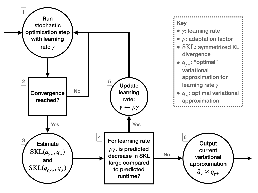
Figure 1: Schematic of the high-level logic of our proposed Robust, Automated, and Accurate BBVI (RAABBVI) algorithm.

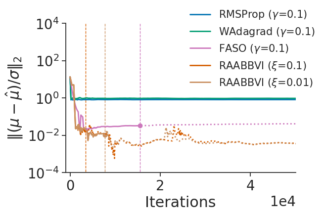
Figure 2: Accuracy comparison of variational inference algorithms using the dogs dataset/model from the posteriordb package (see Section 7.2 for details). Accuracy is measured in terms of relative mean error $\left\|{(\mu-\hat{\mu})/\sigma}\right\|_{2}$, where $\mu$ and $\sigma$ are, respectively, the posterior mean and standard deviation vectors and $\hat{\mu}$ is the variational approximation to $\mu$. The vertical lines indicate the termination points for RAABVI and for fixed–learning-rate automated stochastic optimization (FASO), which is the same as RAABBVI except it always terminates (moves to step 6) after step 4. The fixed-learning rate algorithms has learning rate $\gamma$ and RAABBVI has a user-specified accuracy threshold $\xi$.

In this paper we aim to provide a practical, cohesive, and theoretically well-grounded, optimization framework for BBVI. Our approach builds on a recent line of work inspired by Pflug [46], which uses a fixed learning rate $\gamma$ that is adaptively decreased by a multiplicative factor $\rho$ once the optimization iterates, which form a homogenous Markov chain, have converged [10, 64, 45, 9, 66, 13]. A benefit of this approach is that, for a given learning rate, a dramatically more accurate estimate of the optimal variational parameter can be obtained by using iterate averaging [52, 47, 16]. However, as we have shown in previous work, existing convergence checks can be unreliable and stop too early [13]. Since the learning rate is decreased by a constant multiplicative factor, decreasing it too early can slow down the optimization by an order of magnitude or more. Hence, it is crucial to develop methods that do not prematurely declare convergence. On the other hand, an optimization framework must also provide a termination criterion that triggers when it is no longer worthwhile to decrease the learning rate further, either because the current variational approximation is sufficiently accurate or because further optimization would be too time-consuming.

The key idea that informs our solutions to these challenges is that we want $q_{\gamma*}$, the target variational approximation for learning rate $\gamma$, to be close to the optimal variational approximation $q_{*}$. We measure closeness in terms of symmetrized Kullback–Leibler (KL) divergence $\mathrm{SKL}(q_{*},q_{\gamma*})$ and show that closeness in symmetrized KL divergence can be translated into bounds on other widely used accuracy metrics like Wasserstein distance [28, 5]. Figure 1 summarizes our proposed algorithm, which we call Robust, Automated, and Accurate BBVI (RAABBVI). The primary contributions of this paper are in steps 2, 3, and 4. In step 2, to determine convergence at a fixed step size, we build upon our approach in Dhaka et al. [13], where we establish that the scale-reduction factor $\widehat{R}$ [22, 23, 58], which is widely used to determine convergence of Markov chain Monte Carlo algorithms, can be combined with a Monte Carlo standard error (MCSE) [24, 58] cutoff to construct a convergence criteria. We have improved upon our previous proposal by:

1. adaptively finding the size of the convergence window, which may need to be large for challenging or high-dimensional distributions over the model parameters, and

2. developing a new rigorous MCSE cutoff condition that guarantees the symmetrized KL divergence between $q_{\rho\gamma*}$ and the estimate of $q_{\rho\gamma*}$ obtained via iterate averaging will be small.

In step 3, we leverage recent results that characterize the bias of the stationary distribution of SGD with a fixed learning rate [16] to estimate $\mathrm{SKL}(q_{*},q_{\gamma*})$ and $\mathrm{SKL}(q_{*},q_{\rho\gamma*})$ without access to $q_{*}$. These estimates enable, in step 4, the use of a termination criterion that compares (i) the predicted relative decrease in the KL divergence if the smaller learning $\rho\gamma$ were used and (ii) the predicted computation required to converge with the learning rate $\rho\gamma$. By trading off between (i) and (ii), the criterion enables the user to balance desired accuracy against computational cost. Figure 2 provides an example of the high accuracy and reliability achievable using RAABBVI compared to alternative optimization algorithms and demonstrates how the user can trade off accuracy and computation by adjusting the accuracy threshold $\xi$.

In summary, by drawing on recent developments in theory and methods for fixed–learning-rate stochastic optimization, tools from MCMC methodology and results from functional analysis, RAABBVI delivers a number of benefits:

• it relies on rigorously justified automation techniques, including automatic learning rate adaptation;

• it has an interpretable, user-adjustable accuracy parameter along with a small number of additional intuitive tuning parameters;

• it detects inaccurate estimates of the optimal variational approximation; and

• it can flexibly incorporate additional or future methodological improvements related to variational inference and stochastic optimization.

We demonstrate through synthetic comparisons and real-world model and data examples that RAABBVI provides high-quality black-box approximate inferences. We make RAABBVI available as part of the open source Python package VIABEL.

2 Preliminaries and Background

2.1 Bayesian inference

Let $\theta\in\mathbb{R}^{d}$ denote a parameter vector of interest, and let $x$ denote observed data. A Bayesian model consists of a prior density $\pi_{0}(\mathrm{d}\theta)$ and a likelihood $\ell(x;\theta)$. Together, the prior and likelihood define a joint distribution over the data and parameters. The Bayesian posterior distribution $\pi$ is the conditional distribution of $\theta$ given fixed data $x$, with $x$ suppressed in the notation since it is always fixed throughout this work. To write this conditional, we define the unnormalized posterior density $\pi^{u}(\theta):=\ell(z;\theta)\pi_{0}(\mathrm{d}\theta)$ and the marginal likelihood, or evidence, $Z:=\int\pi^{u}(\mathrm{d}\theta)$. Then the posterior is $\pi:=\pi^{u}/Z.$ Typically, practitioners report posterior summaries, such as point estimates and uncertainties, rather than the full posterior. For $\vartheta\sim\pi$, typical summaries include the mean $m_{\pi}:=\mathbb{E}(\vartheta)$, the covariance $\Sigma_{\pi}:=\mathbb{E}\{(\vartheta-m_{\pi})(\vartheta-m_{\pi})^{\top}\}$, and $[a,b]$ interval probability $I_{\pi,i,a,b}:=\mathbb{P}\left(\vartheta_{i}\in[a,b]\right)=\mathbb{E}\{\mathds{1}(\vartheta_{i}\in[a,b])\}$, where $\mathds{1}(C)$ is equal to one when $C$ is true and zero otherwise.

2.2 Variational inference

In most Bayesian models, it is infeasible to efficiently compute quantities of interest such as posterior means, variances, and quantiles. Therefore, one must use an approximate inference method, which produces an approximation $q$ to the posterior $\pi$. The summaries of $q$ may in turn be used as approximations to the summaries of $\pi$. One approach, variational inference, is widely used in machine learning. Variational inference aims to minimize some measure of discrepancy ${\mathcal{D}_{\pi}(\cdot)}$ over a tractable family $\mathcal{Q}=\{q_{\lambda}:\lambda\in\mathbb{R}^{m}\}$ of approximating distributions [61, 4]:

$$q_{\lambda_{*}}=\operatornamewithlimits{arg\,min}_{q_{\lambda}\in\mathcal{Q}}{\mathcal{D}_{\pi}(q_{\lambda})}.$$ (2)

The variational family $\mathcal{Q}$ is chosen to be tractable in the sense that, for any $q\in\mathcal{Q}$, we are able to efficiently calculate relevant summaries either analytically or using independent and identically distributed samples from $q$.

In variational inference, the standard choice for the discrepancy ${\mathcal{D}_{\pi}(\cdot)}$ is the Kullback–Leibler (KL) divergence $\mathrm{KL}(q\mid\pi):=\int\log\left(\mathrm{d}q/\mathrm{d}\pi\right)\mathrm{d}q$ [3]. Note that the KL divergence is asymmetric in its arguments. The direction ${\mathcal{D}_{\pi}(q)}=\mathrm{KL}(q\mid\pi)$ is most typical in variational inference, largely out of convenience; the unknown marginal likelihood $Z$ appears in an additive constant that does not influence the optimization, and computing gradients requires estimating expectations only with respect to $q\in\mathcal{Q}$, which is chosen to be tractable. Minimizing $\mathrm{KL}(q\mid\pi)$ is equivalent to maximizing the evidence lower bound [ELBO; 3]:

$$\mathsf{ELBO}(q) :=\int\log\left(\frac{\mathrm{d}\pi^{u}}{\mathrm{d}q}\right)\mathrm{d}q.$$ (3)

While numerous other divergences have been used in the literature [e.g., 26, 36, 7, 15, 63, 62], we focus on $\mathrm{KL}(q\mid\pi)$ since it is the most widely used, the default or only choice in widely used frameworks such as Stan, Pyro, and PyMC3, and easiest to estimate when using simple Monte Carlo sampling to approximate the gradient [14].

2.3 Black-box variational inference

Black-box variational inference (BBVI) methods have greatly extended the applicability of variational inference by removing the need for model-specific derivations [12, 48, 34, 56, 40] and enabling the use of more flexible approximation families [33, 54, 44]. This flexibility is a result of using simple Monte Carlo (and automatic differentiation) to approximate the (gradients of the) expectations that define common choices of the discrepancy objective [44, 40]. To estimate the optimal variational parameter $\lambda_{*}$, BBVI methods commonly uses stochastic optimization schemes of the form

$$\lambda^{(k+1)}\leftarrow\lambda^{(k)}-\gamma^{(k)}d^{(k)},$$ (4)

where $d^{(k)}\in\mathbb{R}^{m}$ is the descent direction and $\gamma^{(k)}>0$ is the learning rate (also called the “step size”) at iteration $k$. Standard stochastic gradient descent corresponds to taking $d^{(k)}=\hat{g}^{(k)}$, a (usually unbiased) stochastic estimate of the gradient $g(\lambda^{(k)}):=\nabla_{\lambda^{(k)}}D_{\pi}(q_{\lambda^{(k)}})$. We are particularly interested in adaptive stochastic optimization methods [e.g., 17, 27, 32] that use a smoothed and/or rescaled version of $\hat{g}^{(k)}$ as the descent direction. For example, RMSProp [27] tracks an exponential moving average of the squared gradient, $\nu^{(k+1)}=\beta\nu^{(k)}+(1-\beta)\hat{g}^{(k)}\odot\hat{g}^{(k)}$, which is used to rescale the current stochastic gradient: $d^{(k)}=\hat{g}^{(k+1)}/\mathchoice{{\hbox{$\displaystyle\sqrt{\nu^{(k)}\,}$}\lower 0.4pt\hbox{\vrule height=6.40555pt,depth=-5.12447pt}}}{{\hbox{$\textstyle\sqrt{\nu^{(k)}\,}$}\lower 0.4pt\hbox{\vrule height=6.40555pt,depth=-5.12447pt}}}{{\hbox{$\scriptstyle\sqrt{\nu^{(k)}\,}$}\lower 0.4pt\hbox{\vrule height=4.51389pt,depth=-3.61113pt}}}{{\hbox{$\scriptscriptstyle\sqrt{\nu^{(k)}\,}$}\lower 0.4pt\hbox{\vrule height=3.65277pt,depth=-2.92224pt}}}$. Mean while, Adam [32] tracks an exponential moving average of the gradient $m^{(k+1)}=\beta_{1}m^{(k)}+(1-\beta_{1})\hat{g}^{(k)}$ as well as the squared gradient $\nu^{(k+1)}=\beta_{2}\nu^{(k)}+(1-\beta_{2})\hat{g}^{(k)}\odot\hat{g}^{(k)}$ and used both to rescale the current stochastic gradient: $d^{(k)}=m^{(k)}/\mathchoice{{\hbox{$\displaystyle\sqrt{\nu^{(k)}\,}$}\lower 0.4pt\hbox{\vrule height=6.40555pt,depth=-5.12447pt}}}{{\hbox{$\textstyle\sqrt{\nu^{(k)}\,}$}\lower 0.4pt\hbox{\vrule height=6.40555pt,depth=-5.12447pt}}}{{\hbox{$\scriptstyle\sqrt{\nu^{(k)}\,}$}\lower 0.4pt\hbox{\vrule height=4.51389pt,depth=-3.61113pt}}}{{\hbox{$\scriptscriptstyle\sqrt{\nu^{(k)}\,}$}\lower 0.4pt\hbox{\vrule height=3.65277pt,depth=-2.92224pt}}}$. The benefits of adaptive algorithms include that they tend to be more stable and are scale invariant, so the learning rate can be set in a problem-independent manner.

2.4 Fixed–learning-rate stochastic optimization

If the learning rate is fixed so that $\gamma^{(k)}=\gamma$, then we can view the iterates $\lambda^{(1)},\lambda^{(2)},\dots$ produced by Eq. 4 as a homogenous Markov chain, which under certain conditions will have a stationary distribution $\mu_{\gamma}$ [16, 25]. Stochastic optimization with fixed learning rate exhibits two distinct phases: a transient (a.k.a. warm-up) phase during which iterates make rapid progress towards the optimum, followed by a stationary (a.k.a. mixing) phase during which iterates oscillate around the mean of the stationary distribution, $\bar{\lambda}_{\gamma}:=\int\lambda\,\mu_{\gamma}(\mathrm{d}\lambda)$.

The mean $\bar{\lambda}_{\gamma}$ is a natural target because even if the variance of the individual iterates $\lambda^{(k)}$ means they are far from $\lambda_{*}$, $\bar{\lambda}_{\gamma}$ can be a much more accurate approximation to $\lambda_{*}$. For example, the following result quantifies the bias of standard fixed–learning-rate SGD (Gitman et al. [25] provide similar results for momentum-based SGD algorithms):

Theorem 2.1 (Dieuleveut, Durmus and Bach [16, Theorem 4]).

Under regularity conditions on the objective function and the unbiased stochastic gradients, there exist constant vectors $A,B\in\mathbb{R}^{m}$ such that

$$\bar{\lambda}_{\gamma}-\lambda_{*}=A\gamma+B\gamma^{2}+o(\gamma^{2})$$ (5)

and a matrix $A^{\prime}\in\mathbb{R}^{m\times m}$ such that

$$\int(\lambda-\lambda_{*})(\lambda-\lambda_{*})^{\top}\,\mu_{\gamma}(\mathrm{d}\lambda)=A^{\prime}\gamma+O(\gamma^{2}).$$ (6)

In other words, at stationarity, a single iterate will satisfy $\lambda^{(k)}-\lambda_{*}=O(\gamma^{1/2})$ (with high probability) while its expectation will satisfy $\bar{\lambda}_{\gamma}-\lambda_{*}=O(\gamma)$. Therefore, when the learning rate is small, $\bar{\lambda}_{\gamma}$ is substantially better than $\lambda^{(k)}$ as an estimator for $\lambda_{*}$.

In practice the iterate average (i.e., sample mean)

$$\hat{\lambda}_{\gamma}:=\frac{1}{k^{\mathrm{avg}}}\sum_{k=0}^{k^{\mathrm{avg}}-1}\lambda^{(k^{\mathrm{conv}}+k)}$$ (7)

provides an estimate of $\bar{\lambda}_{\gamma}$, where $k^{\mathrm{conv}}$ is the iteration at which the optimization has reached the stationary phase and $k^{\mathrm{avg}}$ is the number of iterations used to compute the average. Using $\hat{\lambda}_{\gamma}$ as an estimate of $\lambda_{*}$ is known as Polyak–Ruppert averaging [47, 52, 2].

When using iterate averaging, it is crucial to ensure the iterate average accurately approximates $\bar{\lambda}_{\gamma}$. Considering a stationary Markov chain, we can compute the Monte Carlo estimate of the mean of the Markov Chain at stationarity. Then the notion of effective sample size (ESS) aids in quantifying the accuracy of this Monte Carlo estimate. Further, the effective sample size can also be used to define the Monte Carlo standard error (MCSE) when the Markov chain satisfies a central limit theorem. We can efficiently estimate the ESS and also approximate the MCSE (see Section B.1 for details). We denote the estimates of ESS and MCSE using iterates $\lambda^{(k^{\mathrm{conv}}:k)}_{i}$ as $\widehat{\mathrm{ESS}}(\lambda^{(k^{\mathrm{conv}}:k)}_{i})$ and $\widehat{\mathrm{MCSE}}(\lambda^{(k^{\mathrm{conv}}:k)}_{i})$ respectively. Dhaka et al. [13] use the conditions $m^{-1}\sum_{i=1}^{m}\widehat{\mathrm{MCSE}}(\lambda^{(k^{\mathrm{conv}}:k)}_{i})<0.02$ and $\widehat{\mathrm{ESS}}(\lambda^{(k^{\mathrm{conv}}:k)}_{i})>20$ to determine when to stop iterate averaging. However, no rigorous justification is given for the MCSE threshold.

2.5 Automatically scheduling learning rate decreases

A benefit of using a fixed learning rate is that it can be adaptively and automatically decreased once the iterates reach stationarity. For example, if the initial learning rate is $\gamma_{0}$, after reaching stationarity the learning rate can decrease to $\gamma_{1}:=\rho\gamma_{0}$, where $\rho\in(0,1)$ is a user-specified adaptation factor. The process can be repeated: when stationarity is reached at learning rate $\gamma_{t}$, the learning rate can decrease to $\gamma_{t+1}:=\rho\gamma_{t}$. In this way the learning rate is not decreased too early (when the iterates are still making fast progress toward the optimum) or too late (when the accuracy of the iterates is no longer improving). Compare this adaptive approach to the canonical one of setting a schedule such as $\gamma^{(k)}=\triangle/(\bigcirc+k)^{\square}$, which requires the choice of three tuning parameters. These tuning parameters can have a dramatic effect on the speed of convergence, particularly when $\lambda^{(0)}$ is far from $\lambda_{*}$.

The question of how to determine when the stationary phase has been reached has a long history with recent renewed attention [45, 66, 9, 35, 64, 46, 10, 13]. One line of work [64, 35, 66] is based on finding an invariant function that has expectation zero under the stationary distribution of the iterates, then using a test for whether the empirical mean of the invariant function is sufficiently close to zero. An alternative approach developed in Dhaka et al. [13] makes use of the potential scale reduction factor $\widehat{R}$, perhaps the most widely used MCMC diagnostic for detecting stationarity [22, 23, 58]. The standard approach to computing $\widehat{R}$ is to use multiple Markov chains. If we have $J$ chains and $K$ iterates in each chain, then $\widehat{R}:=(\hat{\mathbb{V}}/\hat{\mathbb{W}})^{1/2}$, where $\hat{\mathbb{V}}$ and $\hat{\mathbb{W}}$ are estimates of, respectively, the between-chain and within-chain variances. In the split-$\widehat{R}$ version, each chain is split into two before carrying out the computation above, which helps with detecting non-stationarity [23, 58] and allows for use even when $J=1$. Let $\widehat{R}_{i}(W)$ denote the split-$\widehat{R}$ value computed from $\lambda^{(k-W+1)}_{i},\dots,\lambda^{(k)}_{i}$, the $i$th dimension of the last $W$ iterates. Dhaka et al. [13] uses the stationarity condition $\max_{i}\widehat{R}_{i}(100)<1.1$,

3 Methodological Approach

We now summarize our approach to designing a robust, automatic, and accurate optimization framework for BBVI.

Robustness.

A robust method should not be too sensitive to the choice of tuning parameters. It should also work well on a wide range of “typical” problems. To achieve this we design adaptively schemes for setting parameters such as the window size for detecting convergence that are problem-dependent.

Automation.

An automatic method should require minimal input from the user. Any inputs that are required should be clearly necessary (e.g., the model and the data) or be intuitive to an applied user who is not an expert in variational inference and optimization. Therefore, we require the parameters of any adaptation scheme to either be intuitive or not require adjustment by the user. Examples of intuitive parameters include maximum number of iterations, maximum runtime, and, when defined appropriately, accuracy.

Accuracy.

Since we are focused on the optimization perspective, accuracy corresponds to being close to the optimum. So, for variational inference, the key question is how to measure the accuracy of the variational approximation returned by the optimization algorithm, $\hat{q}_{*}$, as an estimate of the optimal variational approximation $q_{*}:=q_{\lambda_{*}}$. But the answer to this question depends upon choosing an appropriate measure of the discrepancy between $q_{*}$ and the posterior $\pi$. Based on the discussion in Section 2.1, the goal should be for quantities such as $m_{q_{*}}$, $\Sigma_{q_{*}}$, and $I_{q_{*},i,a,b}$ to be close to, respectively, $m_{\pi}$, $\Sigma_{\pi}$, and $I_{\pi,i,a,b}$. The interval probabilities are already on an interpretable scale, so ensuring that $|I_{q,i,a,b}-I_{\pi,i,a,b}|$ is much less than 1 is an intuitive notion of accuracy. Since $\Sigma_{\pi}^{1/2}$ establishes the relevant scale of the problem for means and standard deviations, so it is appropriate to ensure that $\|{\Sigma_{\pi}^{-1/2}(m_{\pi}-m_{q_{*}})}\|_{2}$ and $\|{\Sigma_{\pi}^{-1}(\Sigma_{\pi}-\Sigma_{q_{*}})}\|_{2}=\|{I-\Sigma_{\pi}^{-1}\Sigma_{q_{*}}}\|_{2}$ are much less than 1.

We apply our approach to robustness, accuracy, and automation to design the two core components of a BBVI stochastic optimization framework with automated learning rate scheduling:

1. A termination rule for stopping the optimization once the final approximation is close to the optimal approximation (Section 4).

2. A learning rate scheduler, which must detect stationarity and determine how many iterates to average before decreasing the learning rate (Section 5).

4 Termination Rule

The development of our termination rule will proceed in three steps. First, we will select an appropriate discrepancy measure between distributions. Next, we will design an idealized termination rule based on this discrepancy measure. Finally, we will develop an implementable version of the idealized termination rule that satisfies our criteria for being robust, automatic, and accurate.

4.1 Choice of Accuracy Measure

While we want to choose a discrepancy measure that guarantees the accuracy of mean, covariance, and interval probabilities, ideally it would also guarantee other plausible expectations of interest (e.g., predictive densities) are accurately approximated. The Wasserstein distance provides one convenient metric for accomplishing this goal, and is widely used in the analysis of MCMC algorithms and in large-scale data asymptotics [e.g., 30, 39, 51, 18, 19, 60, 20]. For $p\geq 1$ and a positive-definite matrix $\Sigma\in\mathbb{R}^{d\times d}$, we define the $(p,\Sigma)$-Wasserstein distance between distributions $\eta$ and $\zeta$ as

$$\mathcal{W}_{p,\Sigma}(\eta,\zeta):=\inf_{\omega}\left\{\int\|{\Sigma^{-1/2}(\theta-\theta^{\prime})}\|_{2}^{p}\omega(\mathrm{d}\theta,\mathrm{d}\theta^{\prime})\right\}^{1/p},$$ (8)

where the infimum is over the set of couplings between $\eta$ and $\zeta$; that is, Borel measures $\omega$ on $\mathbb{R}^{d}\times\mathbb{R}^{d}$ such that $\eta=\omega(\cdot,\mathbb{R}^{d})$ and $\zeta=\omega(\mathbb{R}^{d},\cdot)$ [59, Defs. 6.1 & 1.1]. Small $(p,\Sigma)$-Wasserstein distance implies many functionals of the two distributions are close relative to the scale determined by $\Sigma^{1/2}$.

Specifically, we have the following result, which is an immediate corollary of Huggins et al. [28, Theorem 3.4].

Proposition 4.1.

If $\mathcal{W}_{p,\Sigma}(\eta,\zeta)\leq\varepsilon$ for any $p\geq 1$, then

$$\|{\Sigma^{-1/2}(m_{\eta}-m_{\zeta})}\|_{2}\leq\varepsilon$$ (9)

If $\mathcal{W}_{2,\Sigma}(\eta,\zeta)\leq\varepsilon$, then, for $\varrho:=\min\{\left\|{\Sigma^{-1}\Sigma_{\eta}}\right\|_{2}^{1/2},\left\|{\Sigma^{-1}\Sigma_{\zeta}}\right\|_{2}^{1/2}\}$,

$$\|{\Sigma^{-1}(\Sigma_{\eta}-\Sigma_{\zeta})}\|_{2}<2\varepsilon(\varrho+\varepsilon).$$ (10)

More generally, small $(p,\Sigma)$-Wasserstein distance for any $p\geq 1$ guarantees the accuracy of expectations for any function $f$ with small Lipschitz constant with respect the metric $d_{\Sigma}(\theta,\theta^{\prime}):=\|{\Sigma^{-1/2}(\theta-\theta^{\prime})}\|_{2}$ – that is, when $\sup_{\theta\neq\theta^{\prime}}|f(\theta)-f(\theta^{\prime})|/d_{\Sigma}(\theta,\theta^{\prime})$ is small.

While the Wasserstein distance controls the error in mean and covariance estimates, it does not provide strong control on interval probability estimates. The KL divergence, however, does, since for distributions $\eta$ and $\zeta$, $|I_{\eta,i,a,b}-I_{\zeta,i,a,b}|\leq\mathchoice{{\hbox{$\displaystyle\sqrt{\mathrm{KL}(\eta\mid\zeta)/2\,}$}\lower 0.4pt\hbox{\vrule height=7.5pt,depth=-6.00003pt}}}{{\hbox{$\textstyle\sqrt{\mathrm{KL}(\eta\mid\zeta)/2\,}$}\lower 0.4pt\hbox{\vrule height=7.5pt,depth=-6.00003pt}}}{{\hbox{$\scriptstyle\sqrt{\mathrm{KL}(\eta\mid\zeta)/2\,}$}\lower 0.4pt\hbox{\vrule height=5.25pt,depth=-4.20003pt}}}{{\hbox{$\scriptscriptstyle\sqrt{\mathrm{KL}(\eta\mid\zeta)/2\,}$}\lower 0.4pt\hbox{\vrule height=3.75pt,depth=-3.00002pt}}}$ for all $a<b$ and $i$ (see Section B.2). As we show next, in many scenarios we can bound the Wasserstein distance by the KL divergence and therefore enjoy the benefits of both. Our result is based on the following definition, which makes the notion of the scale of a distribution precise:

Definition 4.2.

For $p\geq 1$ and a positive-definite matrix $\Sigma\in\mathbb{R}^{d\times d}$, the distribution $\eta$ is said to be $(p,\Sigma)$-exponentially controlled if

$$\inf_{\theta^{\prime}}\log\int e^{\|{\Sigma^{-1/2}(\theta-\theta^{\prime})}\|_{2}^{p}}\eta(\mathrm{d}\theta)\leq d/2.$$ (11)

Specially, $\Sigma^{1/2}$ establishes the appropriate scale for uncertainty with respect to $\eta$. For example, if $\eta=\mathcal{N}(m,V)$, then it is a straightforward exercise to confirm that $\eta$ is $(2,1.78^{2}V)$-exponentially controlled.

The following result establishes the relevant link between the KL divergence and the Wasserstein distance via Definition 4.2.

Proposition 4.3.

If $\eta$ is $(p,\Sigma)$-exponentially controlled, then for all $\zeta$ absolutely continuous with respect to $\eta$,

$$\mathcal{W}_{p,\Sigma}(\eta,\zeta)\leq(3+d)\mathcal{K}_{p}(\eta\mid\zeta),$$ (12)

where $\mathcal{K}_{p}(\eta\mid\zeta):=\mathrm{KL}(\zeta\mid\eta)^{\frac{1}{p}}+\{\mathrm{KL}(\zeta\mid\eta)/2\}^{\frac{1}{2p}}$.

Proof.

The result follows from Bolley and Villani [5, Corollary 2.3] after the change-of-variable $\theta\mapsto\Sigma^{-1/2}\theta$ and using the fact that the KL divergence is invariant under diffeomorphisms, then applying Eq. 11. ∎

If $\zeta$ and $\eta$ could operate over different scales, then we can use the symmetrized KL divergence $\mathrm{SKL}(\zeta,\eta):=\mathrm{KL}(\zeta\mid\eta)+\mathrm{KL}(\eta\mid\zeta)$. Indeed, it follows from Proposition 4.3 that if $\mathrm{SKL}(\zeta,\eta)$ is small, then the $(p,\Sigma)$-Wasserstein distance is small whenever either $\eta$ or $\zeta$ is $(p,\Sigma)$-exponentially controlled.

4.2 An Idealized Termination Rule

Based on our developments in Section 4.1, we will define our termination rule in terms of the symmetrized KL divergence. Recall that $q_{*}$ denotes the optimal variational approximation to $\pi$ and $\hat{q}_{*}$ denotes an estimate of $q_{*}$. Since total variation and $(1,\Sigma)$-Wasserstein distances are controlled by the square root of the KL divergence, we focused on the square root of the symmetrized KL divergence. For the current learning rate $\gamma>0$, let $q_{\gamma*}:=q_{\bar{\lambda}_{\gamma}}$ denote the target $\gamma$–learning-rate variational approximation. The termination rule we propose is based on the trade-off between the improved accuracy of the approximation if the learning rate were reduced to $\rho\gamma$ and the time required to reach that improved accuracy. To quantify the improved accuracy, we introduce a user-chosen target accuracy target $\xi$ for $\mathrm{SKL}(q_{*},\hat{q}_{*})^{1/2}$. If the user expects $\mathrm{KL}(\pi\mid q_{*})$ to be large, then setting $\xi$ to a moderate value such as 1 or 10 could give acceptable performance. If the user expects $\mathrm{KL}(\pi\mid q_{*})$ to be small, then setting $\xi$ to a value such as 0.1 or 0.01 might be more appropriate. Using $\xi$, define the relative SKL improvement $\mathrm{RSKL}$ as

$$\mathrm{RSKL}:=\frac{\mathrm{SKL}(q_{*},q_{\rho\gamma*})^{1/2}+\xi}{\mathrm{SKL}(q_{*},q_{\gamma*})^{1/2}},$$ (13)

where the first term measures the relative improvement of the approximation if the learning rate were reduced and the second term measures the current accuracy relative to the desired accuracy. To quantify the time to obtain the relative accuracy improvement, we use the number of iterations to reach convergence for the fixed learning rate $\rho\gamma$. Letting $\body_{\gamma*}$ denote the number of iterations required to reach the target $\gamma$–learning-rate variational approximation, we define the relative iteration increase

$$\mathrm{RI}:=\frac{\body_{\rho\gamma*}}{\body_{\gamma*}+\body_{0}},$$ (14)

where $\body_{0}$ denotes a number of iterations the user would consider “small”. Combining $\mathrm{RSKL}$ and $\mathrm{RI}$, we obtain the inefficiency index $\mathcal{I}=\mathrm{RSKL}\times\mathrm{RI}$, the relative improvement in accuracy times the relative increase in runtime. Our idealized SKL inefficiency termination rule triggers when $\mathcal{I}>\tau$, where $\tau$ is a user-specified inefficiency threshold which allows the user to trade off accuracy with computation, but only up to the point where $\mathrm{SKL}(q_{*},q_{\gamma*})^{1/2}\approx\xi$.

4.3 An Implementable Termination Rule

The idealized SKL inefficiency termination rule cannot be directly implemented since $q_{*}$ is unknown – and if it were known, it would be unnecessary to run the optimization algorithm. However, we will show that it is possible to obtain a good estimate of the symmetrized KL divergence between the approximation obtained with a given learning rate $\gamma^{\prime}$ and the optimal approximation without access to $q_{*}$.

Recall that $q_{\gamma*}$ denotes the target $\gamma$–learning-rate variational approximation. With a slight abuse of notation, we let the optimal zero–learning-rate approximation refer to the optimal approximation: $q_{0*}:=q_{*}$. Our approach is motivated by Theorem 2.1 and in particular the form of the bias $\bar{\lambda}_{\gamma}-\lambda_{*}$ in Eq. 5. Our analysis focuses on the still-common setting when $\mathcal{Q}$ is the family of mean-field Gaussian distributions, where the parameter $\lambda=(\tau,\psi)\in\mathbb{R}^{2d}$ corresponds to the distribution $q_{\lambda}=\mathcal{N}(\tau,\operatorname{diag}e^{2\psi})$.

Proposition 4.4.

Let $\mathcal{Q}$ be the family of mean-field Gaussian distributions. If Eq. 5 holds and $\gamma^{\prime}=O(\gamma)$, then there is a constant $C>0$ depending only on $A$ and $\lambda_{*}$ such that

$$\mathrm{SKL}(q_{\gamma*},q_{\gamma^{\prime}*})=C(\gamma-\gamma^{\prime})^{2}+o(\gamma^{2}).$$ (15)

See Section A.1 for the proof. Assuming that the current learning rate is $\gamma$, then the previous learning rate was $\gamma/\rho$. Let $\delta_{\gamma}:=\mathrm{SKL}(q_{\gamma*},q_{\gamma/\rho*})$ denote the symmetrized KL divergence between the optimal variational approximations obtained at each of these learning rates. In principle we can use Proposition 4.4 to estimate $C$ by

$$\hat{C}=\delta_{\gamma}\rho^{2}/\{\gamma^{2}(1-\rho)^{2}\},$$ (16)

and then estimate that

$$\mathrm{SKL}(q_{\gamma*},q_{*})\approx\hat{C}\gamma^{2}=\delta_{\gamma}\rho^{2}/(1-\rho)^{2}.$$ (17)

There are, however, two problems with the tentative approach just outlined. The first problem is that Theorem 2.1 only holds for standard SGD; however, adaptive SGD algorithms are widely used in practice. Indeed, we observe empirically that for RMSProp $\mathrm{SKL}(q_{\gamma*},q_{\gamma^{\prime}*})=\Theta(|\gamma-\gamma^{\prime}|)$ (see Fig. C.6). Our solution is to modify an adaptive gradient method to behave asymptotically like SGD. In the cases of RMSProp and Adam, we propose Averaged RMSProp (avgRMSProp) and Averaged Adam (avgAdam), where

$$\nu^{(k+1)}=\beta_{k}\nu^{(k)}+(1-\beta_{k})\hat{g}^{(k)}\odot\hat{g}^{(k)},$$ (18)

for $\beta_{k}=1-1/k$. Hence, $\nu^{(k+1)}=(k+1)^{-1}\sum_{k^{\prime}=0}^{k}\hat{g}^{(k)}\odot\hat{g}^{(k)}$ is the averaged squared gradient over all iterations [41, §4]. As long as the SGD Markov chain is ergodic and $\mathbb{E}[\hat{g}^{(k)}\odot\hat{g}^{(k)}]<\infty$ at stationarity, $\nu^{(k)}$ converges almost surely to a constant and hence the SGD bias analysis also applies to avgRMSProp and avgAdam.

The second problem is that Proposition 4.4 only holds for the mean-field Gaussian variational family. However, other variational families such as normalizing flows are of substantial practical interest. Therefore, we consider the weaker assumption that either Eq. 5 holds or there exist constant vectors $\Lambda,A\in\mathbb{R}^{m}$ and a constant $\kappa\in[1/2,1)$ such that

$$\bar{\lambda}_{\gamma}=\lambda_{*}+\Lambda\gamma^{\kappa}+A\gamma+o(\gamma^{2\kappa}).$$ (19)

Adding the latter assumption, we have following generalization of Proposition 4.4:

Proposition 4.5.

Let $\mathcal{Q}$ be the family of mean-field Gaussian distributions. If (i) Eq. 19 holds for some $\kappa\in[1/2,1)$ or Eq. 5 holds (in which case let $\kappa=1$), and (ii) $\gamma^{\prime}=O(\gamma)$, then there is a constant $C>0$ such that

$$\mathrm{SKL}(q_{\gamma*},q_{\gamma^{\prime}*})=C\{\gamma^{\kappa}-(\gamma^{\prime})^{\kappa}\}^{2}+o(\gamma^{2\kappa}).$$ (20)

Moreover, $C$ depends on only $\lambda_{*}$ and either $\Lambda$ (if $\kappa\in[1/2,1)$) or $A$ (if $\kappa=1$).

See Section A.2 for the proof. Using Proposition 4.5 and omitting $o(\gamma^{2\kappa})$ terms, we have $\delta_{\gamma}\approx C\gamma^{2\kappa}(1/\rho^{\kappa}-1)^{2}.$ To improve the reliability of the estimates based on Proposition 4.5, we propose to use the symmetrized KL estimates between the variational approximations obtained at successive fixed learning rates. Let $\gamma_{0}$ denote the initial learning rate, so that after $t$ learning rate decreases, the learning rate is $\gamma_{t}:=\gamma_{0}\rho^{t}$. Let $\delta_{t}:=\mathrm{SKL}(q_{\gamma_{t}*},q_{\gamma_{t-1}*})$ and assume the current learning rate is $\gamma_{T}$.

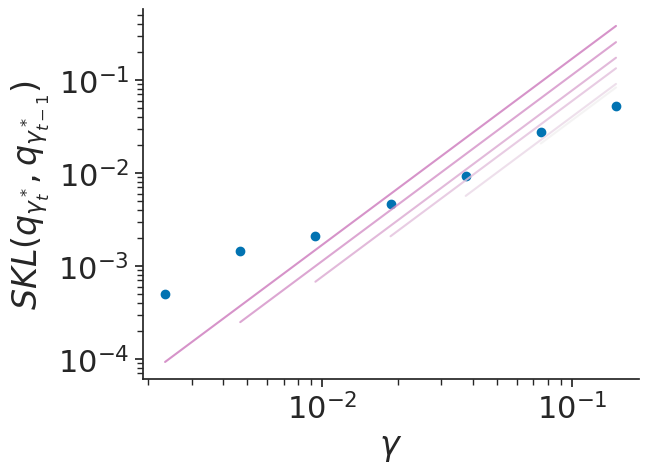
(a)

(b)

Figure 3: Results for estimating the symmetrized KL divergence with avgAdam in the case of a Gaussian distribution $\mathcal{N}(0,V)$ with $d=100$ and $V_{ij}=j\mathds{1}[i=j]$ (diagonal non-identity covariance). (a) Learning rate versus symmetrized KL divergence of adjacent iterate averaged estimates of the optimal variational distribution. The lines indicate the linear regression fits, with setting $\kappa=1$. (b) Square root of true symmetrized KL divergence versus the estimated value with $95\%$ credible interval. The uncertainty of the estimates decreases and remains well-calibrated as the learning rate decreases.

Depending on the optimization algorithm, we can estimate $\kappa$ (or set $\kappa=1$ if using modified adaptive SGD algorithm with a mean-field Gaussian variation family) and $C$ using a regression model of the form

$$\log\delta_{t} =\log C+2\log(1/\rho^{\kappa}-1)+2\kappa\log\gamma_{t}+\eta_{t}, t =1,\dots,T,$$ (21)

where $\eta_{t}\sim\mathcal{N}(0,\sigma^{2})$. Given the estimate $\hat{C}$ for $C$ and the estimate $\hat{\kappa}$ for $\kappa$ (or $\hat{\kappa}=1$) , we obtain the estimated relative SKL,

$$\widehat{\mathrm{RSKL}}=\rho^{\hat{\kappa}}+\frac{\xi}{\hat{C}^{1/2}\gamma_{t}^{\hat{\kappa}}}.$$ (22)

Because we use the regression model in Eq. 21 in a low-data setting, we place priors on $\log C$ and $\sigma$:

$$\log C \sim{\sf{Cauchy}}(0,10), \sigma \sim{\sf{Cauchy}}^{+}(0,10),$$ (23)

where ${\sf{Cauchy}}^{+}$ is the Cauchy distribution truncated to nonnegative values. If we use adaptive SGD algorithm then we also place a prior on $\kappa$:

$$\kappa\sim{\sf{Unif}}(0,1),$$ (24)

for a further generalized version of Proposition 4.5. Also, because we expect early SKL estimates to be less informative about $C$ (and $\kappa$ due to the influence of $o(\gamma^{2\kappa})$ terms), we use a weighted regression with the likelihood term for $(\delta_{t},\gamma_{t})$ having weight

$$w_{t}=\{1+(T-t)^{2}/9\}^{-1/4}.$$ (25)

Given above details, we use dynamic Hamiltonian Monte Carlo (HMC) algorithm and posterior mean(s) to estimate $\hat{C}$ (and $\hat{\kappa}$). Figure 3 validates that, in the case of avgAdam, the log of the learning rate and symmetrized KL divergence have approximately a linear relationship and that our regression approach to estimating $C$ leads to reasonable estimates of $\mathrm{SKL}(q_{\gamma*},q_{*})$. See Fig. C.2 for similar results with other target distributions with avgAdam.

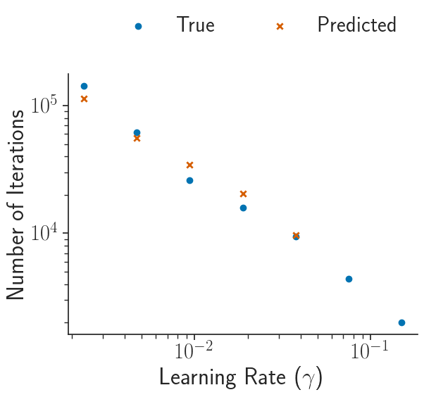
Figure 4: Results for predicting the number of iterations needed to reach convergence at each learning rate decrease in the case of Gaussian distribution $\mathcal{N}(0,V)$ with $d=100$ and $V_{ij}=j\mathds{1}[i=j]$ (diagonal non-identity covariance). The blue points (orange crosses) represent the true (predicted) number of iterations needed to reach convergence.

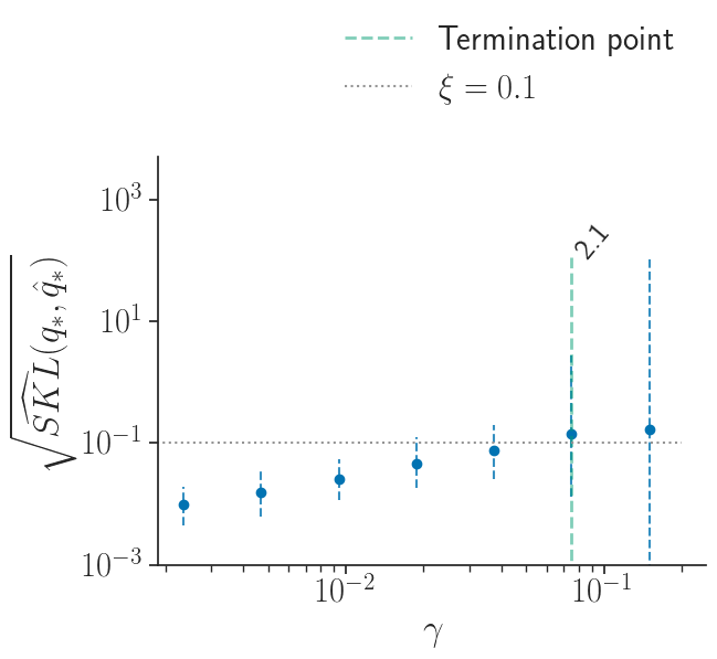
(a)

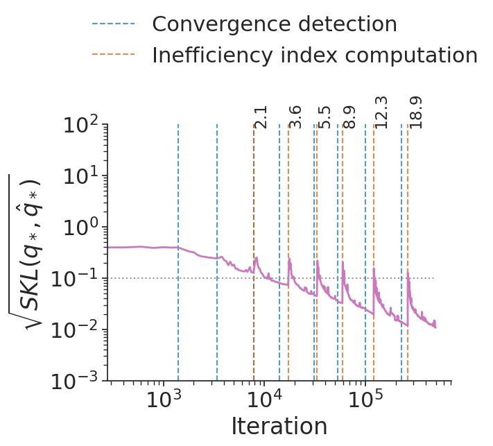
(b)

Figure 5: Results for the termination rule trigger point in the case of a Gaussian distribution $\mathcal{N}(0,V)$ with $d=100$ and $V_{ij}=j\mathds{1}[i=j]$ (diagonal non-identity covariance). (a) Learning rate versus square root of estimated symmetrized KL divergence with 95% credible interval (dashed blue line). The green vertical line indicates the termination rule trigger point with corresponding $\hat{\mathcal{I}}$ value. (b) Iterations versus square root of symmetrized KL divergence between iterate average and optimal variational approximation. The vertical lines indicate the convergence detection points using $\hat{R}$ (blue) and inefficiency index computation ($\hat{\mathcal{I}}$) points (orange) with corresponding values.

To estimate $\mathrm{RI}$ we need to estimate the number of iterations to reach convergence at the next learning rate $\gamma_{t+1}$. It is reasonable to assume that there is a exponential growth in the convergence iterations as the learning rate decreases since stochastic gradients to converge at a polynomial rate [6]. Recall that $\body_{\gamma_{t}}$ is the number of iterations to reach convergence at the current learning rate. We fit a weighted least square regression model of the form

$$\log\body_{\gamma_{t}} =\alpha\log\gamma_{t}+\beta+\nu_{t}, t =1,\dots,T,$$ (26)

where $\nu_{t}\sim\mathcal{N}(0,\sigma_{t}^{2})$. We then use the coefficient estimates $\hat{\alpha}$ and $\hat{\beta}$ to predict the number of iterations required for convergence at the next learning rate to be $\widehat{\body}_{\gamma_{t+1}}:=\gamma_{t+1}^{\hat{\alpha}}e^{\hat{\beta}}$. We use the same weights given in Eq. 25 for observations of the regression model due to the non-linear behavior of the earlier convergence iterate estimates. Figure 4 demonstrates that linear relationship in Eq. 26 does in fact hold and that our weighted least square regression model predicts the number of convergence iterations $\body_{\gamma_{t}}$ quite accurately. The estimated relative iterations is then $\widehat{\mathrm{RI}}=\widehat{\body}_{\gamma_{t+1}}/(\body_{\gamma_{t}}+\body_{0})$.

Using the estimates $\widehat{\mathrm{RSKL}}$ and $\widehat{\mathrm{RI}}$ we obtain the termination rule $\widehat{\mathcal{I}}=\widehat{\mathrm{RSKL}}\cdot\widehat{\mathrm{RI}}>\tau$. Figure 5 shows that, when $\xi=0.1$ (the user chosen target-accuracy), the termination rule triggers when the square root of the symmetrized KL divergence is approximately equal to $\xi$. Figures C.3, C.4 and C.5 shows similar results of other Gaussian targets and posteriordb models and datasets (see Section 7.2 for details).

5 Learning Rate Scheduler

For a fixed learning rate, computing the iterate average $\hat{\lambda}_{\gamma}$ defined in Eq. 7 requires determining the iteration $k^{\mathrm{conv}}$ at which stationarity has been reached and the number of iterations $k^{\mathrm{avg}}$ to use for computing the average. We address each of these in turn.

5.1 Detecting convergence to stationarity

We investigated two approaches to detecting stationarity: the SASA+ algorithm of Zhang et al. [66] and the $\widehat{R}$-based criterion from Dhaka et al. [13]. We made several adjustments to both approaches to reduce the number of tuning parameters and to make the remaining ones more intuitive. We found empirically that the $\widehat{R}$ criterion outperformed the SASA+ criterion, so we describe the former here and the latter in Section B.3.

Let $\widehat{R}(\lambda^{(k-W+1)}_{i},\dots,\lambda^{(k)}_{i})$ denote the split-$\widehat{R}$ of the $i$th component of the last $W$ iterates and define

$$\widehat{R}_{\max}(W):=\max_{1\leq i\leq m}\widehat{R}(\lambda^{(k-W+1)}_{i},\dots,\lambda^{(k)}_{i}).$$ (27)

An $\widehat{R}_{\max}(W)$ value close to 1 indicates the last $W$ iterates are close to stationarity. In MCMC applications having $\widehat{R}_{\max}(W)\leq 1.01$ is desirable [57, 58]. Dhaka et al. [13] uses the weaker condition $\widehat{R}_{\max}(W)\leq 1.1$ since iterate averaging does not require the same level of precision as MCMC. Dhaka et al. [13] took the window size $W=100$, but in more challenging and high-dimensional problems a fixed $W$ is insufficient. Therefore, we instead search over window sizes between a minimum window size $W_{\min}$ and $0.95k$ to find the one that minimizes $\widehat{R}_{\max}(W)$. The minimum window size is necessary to ensure the $\widehat{R}$ values are reliable. We use the upper bound $0.95k$ to always allow a small amount of “warm-up” without sacrificing more than 5% efficiency. Therefore, we estimate $W_{\mathrm{opt}}=\operatornamewithlimits{arg\,min}_{W_{\min}\leq W\leq 0.95k}\widehat{R}_{\max}(W)$ using a grid search over 5 equally spaced values ranging from $W_{\min}$ to $0.95k$ and require $\widehat{R}_{\max}(W_{\mathrm{opt}})\leq 1.1$ as the stationarity condition.

Figure 6 compares our adaptive SASA+ and adaptive $\widehat{R}$ criteria to the $\Delta$ELBO rule from Kucukelbir et al. [34], which is used Stan’s ADVI implementation (cf. the results of Dhaka et al. [13]). Additionally, it compares to another convergence detection approach proposed by Pesme, Dieuleveut and Flammarion [45], where they used a distance based statistics to detect the convergence, described in Section B.4. While adaptive SASA+, $\Delta$ELBO, and the distance-based statistic approach sometimes trigger too early or too late, adaptive $\widehat{R}$ consistently triggers when the full window suggests convergence has been reached. See Fig. C.1 for additional Gaussian target examples.

5.2 Determining the number of iterates for averaging

After detecting convergence to stationarity, we need to find $k^{\mathrm{avg}}$ large enough to ensure the iterative average is sufficiently close to the mean $\bar{\lambda}_{\gamma_{t}}$. But what is close enough? Building on our discussion in Section 3, we aim to ensure the error in the variational parameter estimates are small relative to the scale of uncertainty. For mean-field Gaussian distributions, the following result allows us to make such a guarantee precise.

Proposition 5.1.

Let $\mathcal{Q}$ be the family of mean-field Gaussian distributions. Let $\hat{\lambda}=(\hat{\tau},\hat{\psi})$ denote an approximation to $\bar{\lambda}=(\bar{\tau},\bar{\psi})$. Define $\hat{\sigma}:=\exp(\hat{\psi})$ and $\bar{\sigma}:=\exp(\bar{\psi})$. If there exists $\varepsilon\in(0,1/2)$ such that $|\hat{\tau}_{i}-\bar{\tau}_{i}|\leq\varepsilon\hat{\sigma}_{i}$ and $|\hat{\psi}_{i}-\bar{\psi}_{i}|\leq\varepsilon$, then

$$\frac{|\hat{\sigma}_{i}-\bar{\sigma}_{i}|}{\bar{\sigma}_{i}} \leq 1.5\varepsilon \frac{|\hat{\tau}_{i}-\bar{\tau}_{i}|}{\bar{\sigma}_{i}} \leq 1.75\varepsilon.$$ and (28)

See Section A.4 for the proof. Based on Proposition 5.1, for mean-field Gaussian variational family we use the iterate average once the mean MCSEs $d^{-1}\sum_{i=1}^{d}\mathrm{MCSE}(\hat{\tau}_{\gamma,i})/\hat{\sigma}_{\gamma,i}$ and $d^{-1}\sum_{i=1}^{d}\mathrm{MCSE}(\hat{\psi}_{\gamma,i})$ are less than $\varepsilon_{t-1}$. For other variational families we rely on the less rigorous condition that $m^{-1}\sum_{i=1}^{m}\mathrm{MCSE}(\hat{\lambda}_{\gamma,i})$ is less than $\varepsilon_{t-1}$. We also require the effective sample sizes of all parameters to be at least 50 to ensure the MCSE estimates are reliable.

Because the MCSE check requires computing $d$ ESS values, for high-dimensional models the computational cost can be significant. Therefore, it is important to optimize when the checks are carried out. A well-known approach in such situations is the “doubling trick.” Let $W_{\mathrm{conv}}$ denote the window size when convergence is detected, and let $W_{\mathrm{opt}}$ denote the minimal window size that would result in the MCSE check being satisfied. The doubling trick would suggest checking at iteration numbers $k^{\mathrm{conv}}+2^{j}W_{\mathrm{conv}}$ for $j=0,1,\dots$, in which case the total computational cost is within a factor of $4\log W_{\mathrm{opt}}$ of the optimal scenario in in which the check is only done at $k^{\mathrm{conv}}+W_{\mathrm{conv}}$ and $k^{\mathrm{conv}}+W_{\mathrm{opt}}$). However, we can potentially do substantially better by accounting for the different computational cost of the optimization versus the MCSE check.

Proposition 5.2.

Assume that the cost of the MCSE check using $K$ iterates is $C_{E}K$ and the cost of $K$ iterations of optimization is $C_{O}K$. Let $r:=C_{O}/C_{E}$, $\chi(r):=1+(1+r)^{-1/2}$, and $g(r):=(2+r+2r^{1/2})/(1+r)$. If the MCSE check is done on iteration numbers $k^{\mathrm{conv}}+\chi(r)^{j}W_{\mathrm{conv}}$ for $j=0,1,\dots$, then the total computational cost will be within a factor of $g(r)$ of optimal.

See Section A.5 for the proof. Since $g(0)=4$ and $g(r)$ is monotonically decreasing in $r$, when $r\approx 0$ – that is, $C_{O}$ is negligible compared to $C_{E}$ – we recover the doubling rule since $\chi(0)=2.$ However, as long as $r$ is significantly greater than zero, the worst-case additional cost factor can be substantially less than 4. Therefore we carry out the MCSE check on iteration numbers $k^{\mathrm{conv}}+\chi(r)^{j}W_{\mathrm{conv}}$ with $r$ estimated based on the actual runtimes of the optimization so far and the first MCSE check.

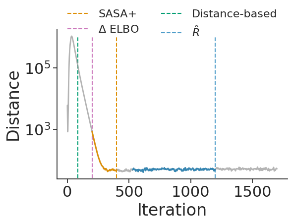
(a)

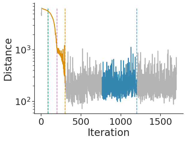
(b)

Figure 6: Iteration number versus distance between iterate average and current iterate. The vertical lines indicate convergence detection trigger points and (for SASA+ and $\widehat{R}$) the colored portion of the accuracy values indicate they are part of the window used for convergence detection. (a) An uncorrelated Gaussian distribution $\mathcal{N}(0,V)$ with $d=500$ and $V=I$. (b) A posteriordb dataset/model mcycle_gp with $d=66$.

6 Complete Framework

Combining our innovations from Sections 4 and 5 leads to our complete framework. When $\gamma$ is fixed, our proposal from Section 5 is summarized in Algorithm 1, which we call Fixed–learning-rate Automated Stochastic Optimization (FASO). Combining the termination rule from Section 4 with FASO, we get our complete framework, Robust, Automated, and Accurate Black-box Variational Inference (RAABBVI), which we summarize in Algorithm 2. We will verify the robustness of RAABBVI through numerical experiments. Accuracy is guaranteed by the symmetrized KL divergence termination rule and the MCSE criterion for iterate averaging. RAABBVI is automatic since the user is only required to provide a target distribution and the only tuning parameter we recommend changing from their defaults are defined on interpretable, intuitive scales:

• accuracy threshold $\xi$: The symmetrized KL divergence accuracy threshold can be set based on the expected accuracy of the variational approximation. If the user expects $\mathrm{KL}(\pi\mid q_{*})$ to be large, then we recommend choosing $\xi\in[1,10]$. If the user expects $\mathrm{KL}(\pi\mid q_{*})$ to be fairly small, then we recommend choosing $\xi\in[.01,1]$. Our experiments suggest $\xi=0.1$ is a good default value.

• inefficiency threshold $\tau$: We recommend setting inefficiency threshold $\tau=1$, as this weights accuracy and computation equally. A larger value (e.g., 2) could be chosen if accuracy is more important while a smaller value (e.g., 1/2) would be appropriate if computation is more of a concern.

• maximum number of iterations $K_{\max}$: The maximum number of iterations can be set by the user based on their computational budget. RAABBVI will warn the user if the maximum number of iterations is reached without convergence, so the user can either increase $K_{\max}$ or accept the estimated level of accuracy that has been reached.

We expect the remaining tuning parameters will typically not be adjusted by the user. We summarize our recommendations:

• initial learning rate $\gamma_{0}$: When using adaptive methods such as RMSProp or Adam, the initial learning rate can essentially be set in a problem-independent manner. We use $\gamma_{0}=0.3$ in all of our experiments. If using non-adaptive methods, a line search rule such as the one proposed in Zhang et al. [66] could be used to find a good initial learning rate.

• minimum window size $W_{\min}$: We recommend taking $W_{\min}=200$ so that that each of the split-$\widehat{R}$ values are based on at least 100 samples.

• small iteration number $\body_{0}$: The value of $\body_{0}$ should represent a number of iterations the user considers to be fairly small (that is, not requiring too much computational effort). We use $\body_{0}=5W_{\mathrm{min}}=1000$ for our experiments, but it could be adjusted by the user.

• initial iterate average relative error threshold $\varepsilon_{0}$: We recommend scaling $\varepsilon_{0}$ with $\xi$ since more accurate iterate averages are required for sufficiently accurate symmetrized KL estimates. Therefore, we take $\varepsilon_{0}=\xi$ by default.

• adaptation factor $\rho$: We recommend taking $\rho=0.5$ because having smaller $\rho$ value could lead to a few $\delta_{t}$ values to estimate $C$ and $\kappa$ and having larger $\rho$ value will make algorithm too slow.

• Monte Carlo samples $M$: We find that $M=10$ provides a good balance between gradient accuracy and computational burden but the performance is fairly robust to the choice of $M$ as long as it is not too small.

7 Experiments

Unless stated otherwise, all experiments use avgAdam to compute the descent direction, mean-field Gaussian distributions as the variational family, and the tuning parameters values recommended in Section 6. We fit the regression model for $C$ (and $\kappa$) in Stan, which resulted in extremely small computational overhead of less than $0.5\%$. We compare RAABBVI to FASO and fixed–learning rate versions of RMSProp and a windowed version of Adagrad (WAdagrad), which the default optimizer in PyMC3. We run all the algorithms that do not have a termination criterion for $K_{\max}=100{,}000$ iterations and for the fixed–learning-rate algorithms we use learning rate $\gamma=0.1$. We use symmetrized KL divergence as the accuracy measure when we can compute the ground-truth optimal variational approximation. Otherwise, we use relative mean error $\left\|{(\mu-\hat{\mu})/\sigma}\right\|_{2}$ and relative standard deviation error $\left\|{\hat{\sigma}/\sigma-1}\right\|_{2}$, where $\mu$ and $\sigma$ are, respectively, the posterior mean and standard deviation vectors and $\hat{\mu}$ and $\hat{\sigma}$ are the variational approximations to, respectively, $\mu$ and $\sigma$.

Input: initial variational parameter $\lambda^{(0)}$,
learning rate $\gamma$,
minimum window size $W_{\min}$,
iterate average relative error threshold $\varepsilon$,
maximum iterations $K_{\max}$

$k^{\mathrm{conv}}\leftarrow\mathbf{null}$

 // iteration when stationarity reached

1 $\mathit{success}\leftarrow\mathbf{false}$

2 for $k=1,\dots,K_{\max}$ do

3       compute stochastic gradient $\hat{g}^{(k)}$

4       compute descent direction $d_{k}$

      

       // step in descent direction

5       $\lambda^{(k+1)}\leftarrow\lambda^{(k)}-\gamma d_{k}$

6       if $k^{\mathrm{conv}}=\mathbf{null}$ and $k\mod k_{\mathrm{check}}=0$  then check for convergence

            

             // define window-based ESS

7             $\widehat{R}_{\max}(W):=\max_{1\leq i\leq m}\widehat{R}(\lambda^{(k-W+1)}_{i},\dots,\lambda^{(k)}_{i})$

            

             // compute optimal window

8             $W_{\mathrm{opt}}\leftarrow\operatornamewithlimits{arg\,min}_{W_{\min}\leq W\leq 0.95k}\widehat{R}_{\max}(W)$

9             if $\widehat{R}_{\max}(W_{\mathrm{opt}})\leq 1.1$ then

10                   $k^{\mathrm{conv}}\leftarrow k-W_{\mathrm{opt}}$

                  

                   // window size at which to check MCSE

11                   $W_{\mathrm{check}}\leftarrow W_{\mathrm{opt}}$

                   $\chi_{*}\leftarrow\chi(r)$

                   // see Prop. 5.2

12                  

13            

14      if $k^{\mathrm{conv}}\neq\mathbf{null}$ and $k-k^{\mathrm{conv}}=W_{\mathrm{check}}$ then check for accuracy of iterate average

15             $W\leftarrow W_{\mathrm{check}}$

16             $\hat{\lambda}\leftarrow W^{-1}\sum_{i=k-W+1}^{k}\lambda^{(i)}$

17             $e\leftarrow\mathrm{MCSE}(\lambda^{(k-W)},\dots,\lambda^{(k)})$

18             $\mathrm{ESS}_{\min}\leftarrow\min_{i}\mathrm{ESS}(\lambda^{(k-W)}_{i},\dots,\lambda^{(k)}_{i})$

19             if mean-field Gaussian family then  $e_{i}\leftarrow e_{i}/\exp(\hat{\psi}_{i})$ for $i=1,\dots,d$

20             if $\mathrm{mean}\ e_{i}<\varepsilon$ and $\mathrm{ESS}_{\min}\geq 50$ then

21                   $\mathit{success}\leftarrow\mathbf{true}$

22                   break

23                  

24            else

25                   $W_{\mathrm{check}}\leftarrow\chi_{*}W$

26                  

27            

28      

29$\hat{\lambda}\leftarrow W^{-1}\sum_{i=k-W+1}^{k}\lambda^{(i)}$

return $(k,\bar{\lambda},\mathit{success})$

Algorithm 1 Fixed–learning-rate Automated Stochastic Optimization (FASO)

Input: initial variational parameter $\lambda^{(0)}$,
maximum number of iterations $K_{\max}$,
initial learning rate $\gamma_{0}$ (default: 0.3),
minimum window size $W_{\min}$ (default: 200),
accuracy threshold $\xi$ (default: 0.1),
inefficiency threshold $\tau$ (default: 1.1),
iterate average error threshold $\varepsilon$ (default: 0.1),
adaptation factor $\rho$ (default: 0.5)
expected convergence iterations $\body_{0}$ (default: 1000)

$\bar{\lambda}_{\mathrm{curr}}\leftarrow\lambda^{(0)}$

 // current iterate average

$\gamma\leftarrow\gamma_{0}$

 // learning rate

$k\leftarrow 0$

 // total iterations

$t\leftarrow 0$

 // total epochs

1 while $k<K_{\max}$ do

       $\bar{\lambda}_{\mathrm{prev}}\leftarrow\bar{\lambda}_{\mathrm{curr}}$

       // record previous iterate average

2       $k_{\mathrm{new}},\bar{\lambda}_{\mathrm{curr}},\mathit{success}\leftarrow$ FASO($\bar{\lambda}_{\mathrm{curr}},\gamma,W_{\min},\varepsilon,K_{\max}-k$)

3       if $\operatorname{not}\mathit{success}$ then

4             print “Warning: failed to converge. Estimated error is $\mathit{error}$”

5             break

6            

      $k\leftarrow k+k_{\mathrm{new}}$

       // update total iterations

7       if $t\geq 1$ then

8             $\delta_{t}\leftarrow\mathrm{SKL}(q_{\bar{\lambda}_{\mathrm{prev}}},q_{\bar{\lambda}_{\mathrm{curr}}})$

9             compute estimates $\hat{C}$ and $\hat{\kappa}$ using weighted linear regression

10             $\widehat{\mathrm{RSKL}}\leftarrow\rho^{\hat{\kappa}}+\xi/(\hat{C}^{1/2}\gamma^{\hat{\kappa}})$

11             $\hat{\body}_{\gamma}\leftarrow k_{\mathrm{new}}^{(t)}-k_{\mathrm{new}}^{(t-1)}$

12             if $t\geq 2$ then

                  

                   // remove the converged iterations of initial variation parameter

13                   compute estimates $\hat{\alpha}$ and $\hat{\beta}$ using weighted least squares

14                   if $\hat{\beta}<0$ then

15                         $\hat{\body}_{\rho\gamma}\leftarrow(\rho\gamma)^{\hat{\alpha}}e^{\hat{\beta}}$

16                        

17                  else

18                         $\hat{\body}_{\rho\gamma}\leftarrow\hat{\body}_{\gamma}$

19                        

20                  $\widehat{\mathrm{RI}}\leftarrow\hat{\body}_{\rho\gamma}/(\hat{\body}_{\gamma}+\body_{0})$

21                   if $\widehat{\mathrm{RSKL}}\cdot\widehat{\mathrm{RI}}>\tau$ then

22                         break

23                  

24            

      $\gamma\leftarrow\rho\gamma$

       // decrease learning rate

       $t\leftarrow t+1$

       // increment epoch counter

25      

return $\bar{\lambda}_{\mathrm{curr}}$

Algorithm 2 Robust, automated, and accurate black-box variational inference (RAABBVI)

7.1 Accuracy with Gaussian Targets

First, to explore optimization accuracy relative to the optimal variational approximation, we consider Gaussian targets of the form $\pi=\mathcal{N}(0,V)$. In such cases we can compute the ground-truth optimal variational approximation either analytically (because the distribution belongs to the mean-field variational family and hence $q_{*}=\pi$) or numerically using deterministic optimization (since the KL divergence between Gaussians is available in closed-form). Specifically, we consider the covariances $V=I$ (identity covariance), $V_{ij}=j\mathds{1}[i=j]$ (diagonal non-identity covariance), $V_{ij}=\mathds{1}[i=j]+0.8\mathds{1}[i\neq j]$ (uniform covariance with correlation 0.8), and $V_{ij}=\mathds{1}[i=j]+0.8^{\mid i-j\mid}\mathds{1}[i\neq j]$ (banded covariance with maximum correlation 0.8).

Figure 7 shows the comparison between RAABBVI and fixed-learning rate versions of RMSProp, Windowed Adagrad (WAdagrad), and FASO. The results indicate that RAABBVI performs well when compared with fixed-learning rate approaches. Moreover, by varying the accuracy threshold $\xi$, the quality of the final approximation $\hat{q}_{*}$ also varies such that $\mathrm{SKL}(q_{*},\hat{q}_{*})^{1/2}\approx\xi$.

To demonstrate the flexibility of our framework, we used RAABBVI with a variety of optimization methods: RMSProp, avgRMSProp, avgAdam, natural gradient descent (NGD), and stochastic quasi-Newton (SQN). See Sections B.6 and B.5 for details. Figure C.7 shows that avgAdam and avgRMSProp optimization methods have a similar improvement in symmetrized KL divergence between optimal and estimated variational approximation for all cases. NGD is not stable for the diagonal non-identity covariance structure and SQN does not perform well with uniform covariance structure. Even though RMSProp shows an improvement in accuracy for large step sizes, accuracy does not improve as the step size decreases.

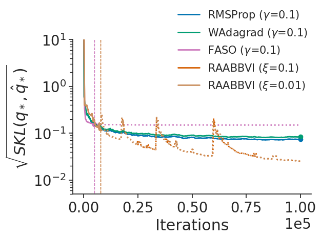
(a) uncorrelated $d=100$

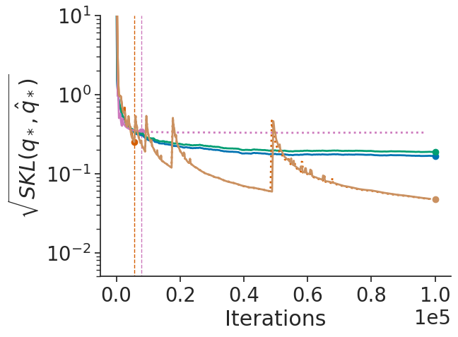
(b) uncorrelated $d=500$

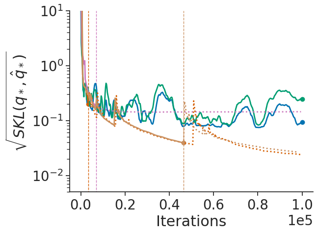
(c) uniform correlated $d=100$

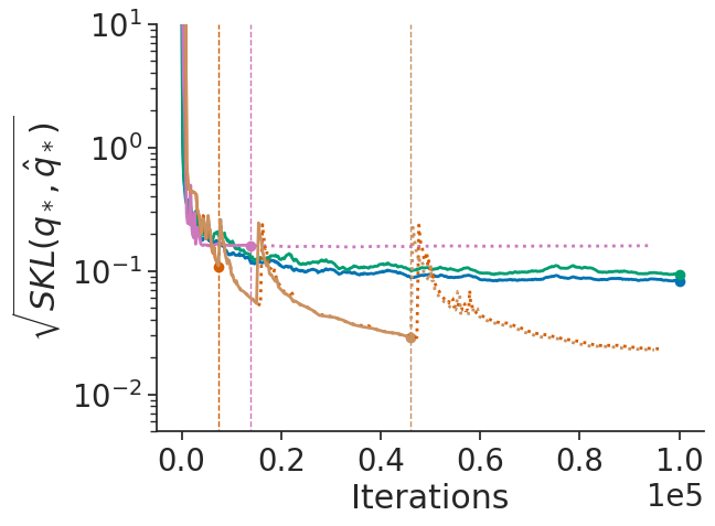
(d) banded correlated $d=100$

Figure 7: Accuracy comparison of variational inference algorithms using Gaussian targets, where accuracy is measured in terms of square root of symmetrized KL divergence between iterate average and optimal variational approximation. The vertical lines indicate the termination rule trigger points of FASO and RAABBVI. Iterate averages for RMSProp and WAdagrad computed at every 200th iteration using a window size of 20% of iterations.

7.2 Reliability Across Applications

To validate the robustness and reliability of RAABBVI across a realistic use cases, we consider 18 diverse dataset/model pairs found in the posteriordb package (see Table C.1 for details). The accuracy was computed based on ground-truth estimates obtained using the posterior draws included in posteriordb package if available. Otherwise, we ran Stan’s dynamic HMC algorithm [55] to obtain the ground truth (4 chains for 50,000 iterations each). To stabilize the optimization, we initialize the variational parameter estimates using RMSProp for the initial learning rate only. A comparison across optimization methods validates our choice of avgAdam over alternatives (Fig. C.8).

Accuracy and robustness.

First we investigate the accuracy and algorithmic robustness of RAABBVI. In terms of robustness, Figures 8, C.10 and C.11 validate our termination criteria since after reaching the termination point there is no considerable improvement of the accuracy for most of the models and datasets. While in many cases the mean estimates are quite accuracy, the standard deviation estimates tended to be poor, which is consistent with typical behavior of mean-field approximations. To examine whether RAABBVI can achieve more accurate results with a more flexible variational family, we conduct the same experiment using multivariate Gaussian approximation family. In some cases the accuracy of the mean and/or standard deviations estimates improve (bball_0, dogs_log, 8schools_c, hudson_lynx, hmm_example, nes2000, and sblrc). However, the results are inconsistent and sometimes worse due to the higher-dimensional, more challenging optimization problem. Overall, the results highlight the need to complement improved an optimization framework such as RAABBVI with posterior approximation accuracy diagnostics.

Comparison to MCMC.

We additionally benchmarked the runtime and accuracy of RAABBVI to Stan’s dynamic HMC algorithm, for which we ran 1 chain for 25,000 iterations including 5,000 warmup iterations. We measure runtime in terms of number of likelihood evaluations. Figures C.12, C.13 and 9 show that RAABBVI tend to result similar or better posterior mean estimates (the exceptions are gp_pois_regr, hudson_lynx, and sblrc). However, the RAABBVI standard deviation estimates tend to be less accurate even when using the full-rank Gaussian variational family.

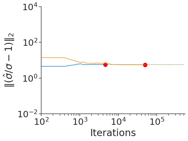
(a) arK

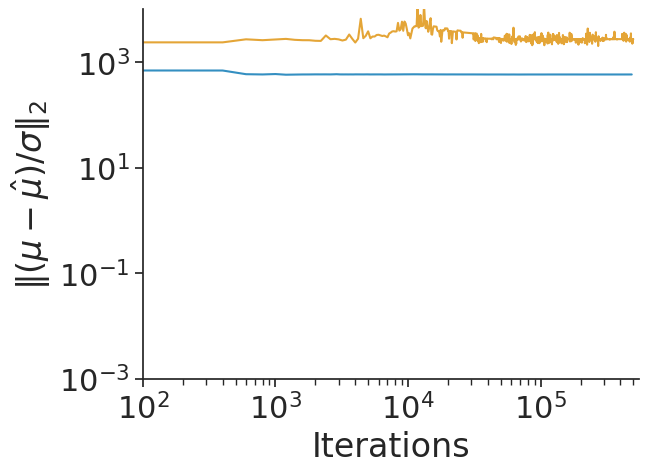
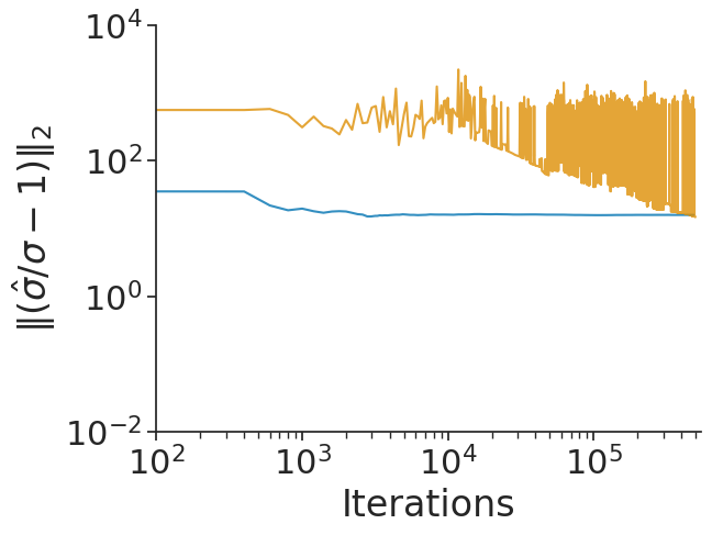
(b) diamonds

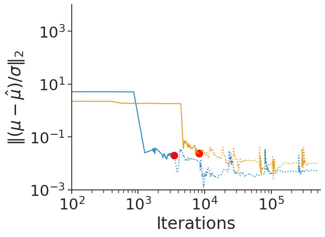
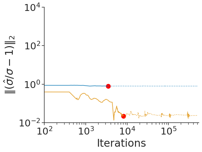
(c) dogs

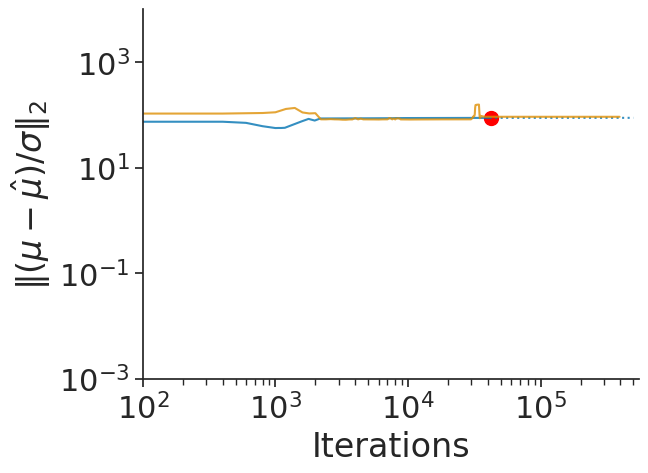
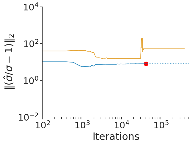
(d) gp_pois_regr

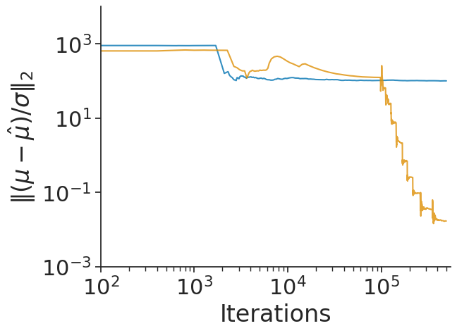
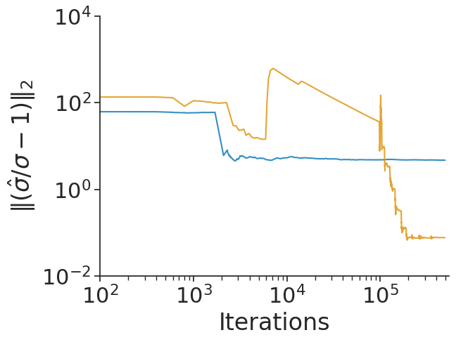
(e) sblrc

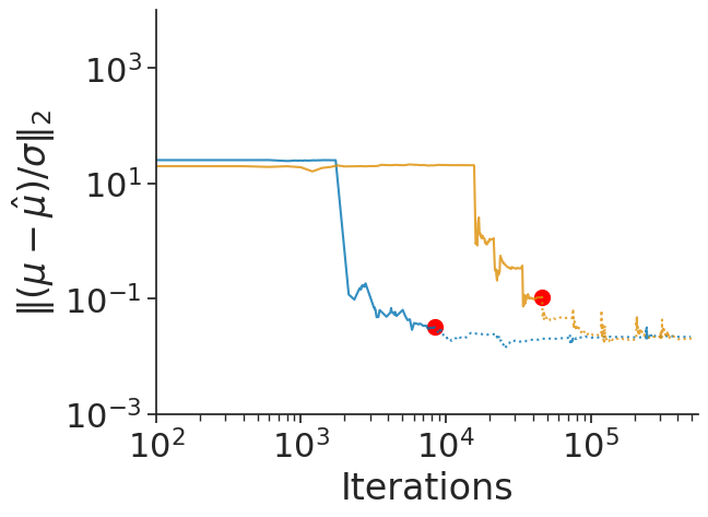
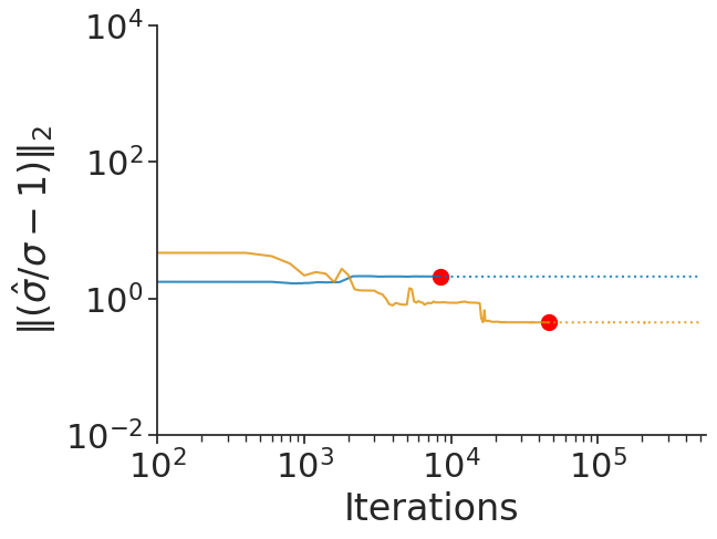
(f) nes2000

Figure 8: Accuracy of mean-field (blue) and full-rank (orange) Gaussian family approximations for selected posteriordb data/models, where accuracy is measured in terms of relative mean error (top) and relative standard deviation error (bottom). The red dots indicate where the termination rule triggers.

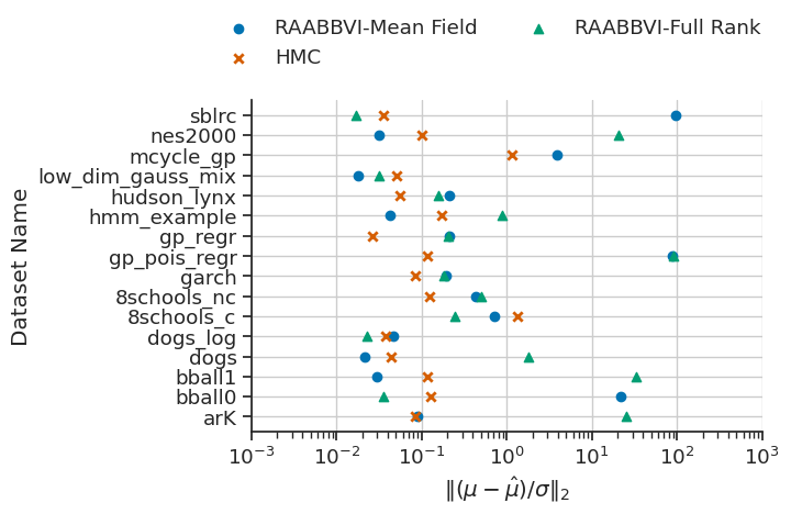
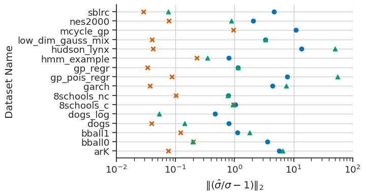
Figure 9: Results of RAABBVI with mean-field Gaussian and full-rank Gaussian family comparison to dynamic HMC in terms of relative mean error (top) and relative standard deviation error (bottom).

7.3 Robustness to Tuning Parameters: Ablation Study

To validate the robustness of RAABBVI to different choices of algorithm tuning parameters, we consider the Gaussian targets and the dogs dataset/model. We vary one tuning parameter while keeping the recommended default values for all others. We consider the following values for each parameter (default in bold):

• initial learning rate $\gamma_{0}$: $0.01,0.1,\mathbf{0.3},0.5$

• minimum window size $W_{\min}$: $100,\mathbf{200},300,500$

• initial iterate average relative error threshold $\varepsilon_{0}$: $0.05,\mathbf{0.1},0.2,0.5$

• inefficiency threshold $\tau$: $0.1,0.5,\mathbf{1.0},1.2$

• Monte Carlo samples $M$: $1,5,\mathbf{10},15,25$.

We repeat each experimental condition 10 times to verify robustness to different initializations of the variational parameters. Figures 10, 11, C.14, C.15, C.16, C.17 and C.18 suggest that overall the accuracy and runtime of RAABBVI is not too sensitive to the choice of the tuning parameters. However, extreme tuning parameter choices (e.g., $\gamma=0.01$ or $M\leq 5$) can lead to longer runtimes.

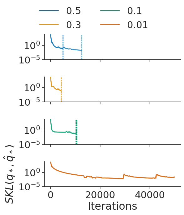
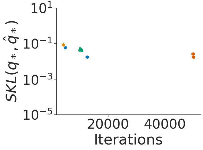
(a) $\gamma_{0}$

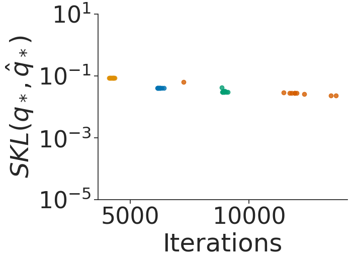
(b) $W_{min}$

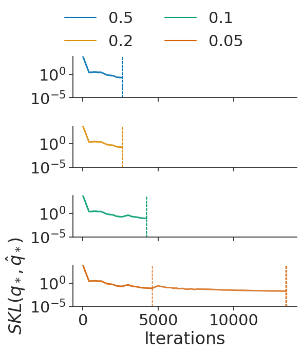
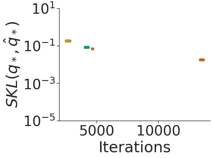
(c) $\varepsilon_{0}$

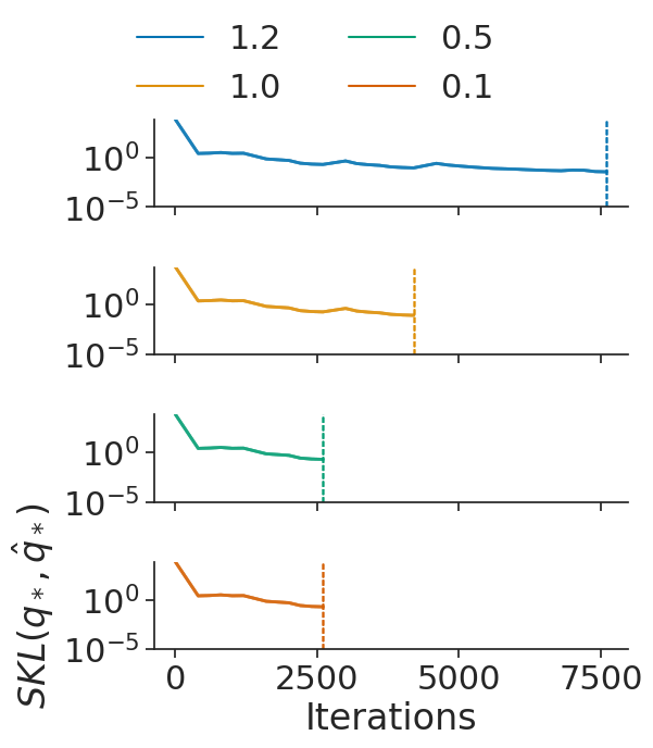
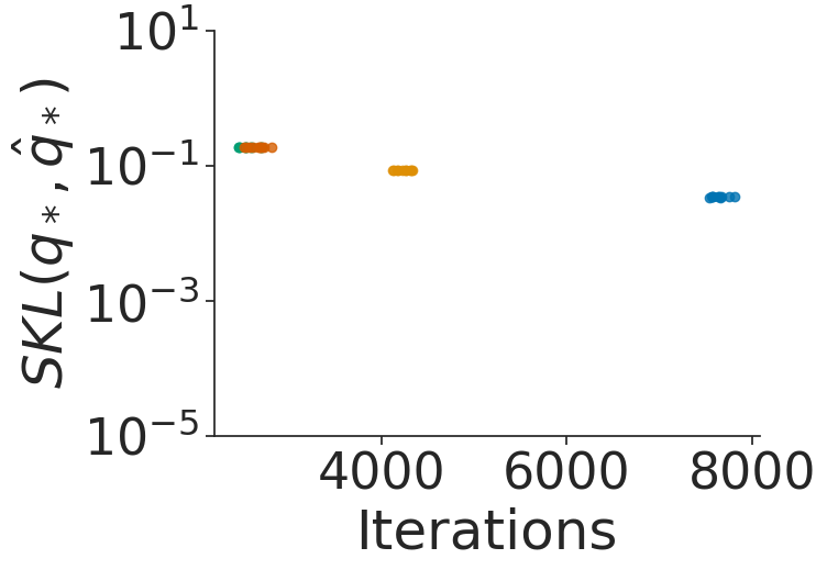
(d) $\tau$

Figure 10: Robustness to tuning parameters (a) initial learning rate $\gamma_{0}$, (b) minimum window size $W_{\min}$, (c) initial iterate average relative error threshold $\varepsilon_{0}$, and (d) inefficiency threshold $\tau$. Results use Gaussian target $\mathcal{N}(0,V)$ with $d=100$ and $V=I$ (identity covariance). (top) Iterations versus symmetrized KL divergence between iterate average and optimal variational approximation. The distinct lines represent repeated experiments and the vertical lines indicate the termination rule trigger points. (bottom) Iterations versus symmetrized KL divergence between iterate average and optimal variational approximation at the termination rule trigger point.

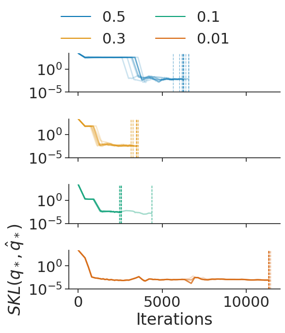
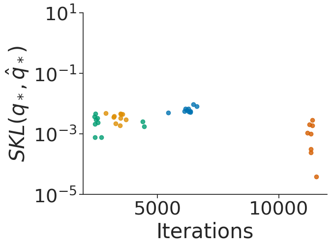
(a) $\gamma_{0}$

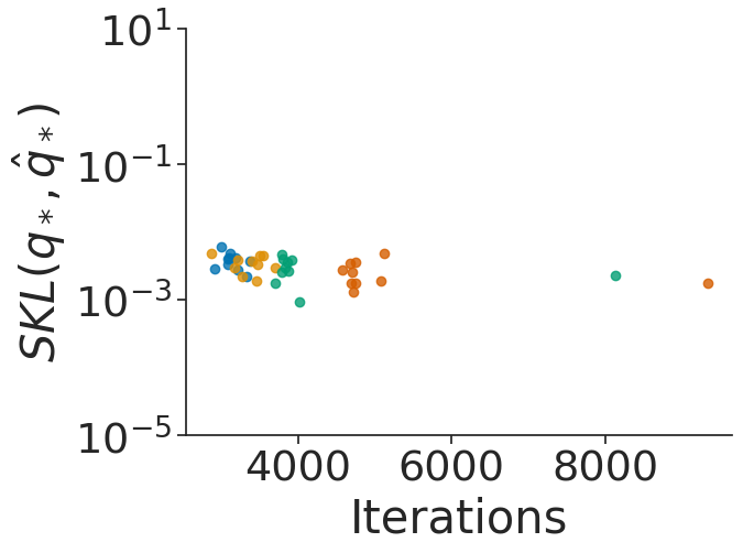
(b) $W_{min}$

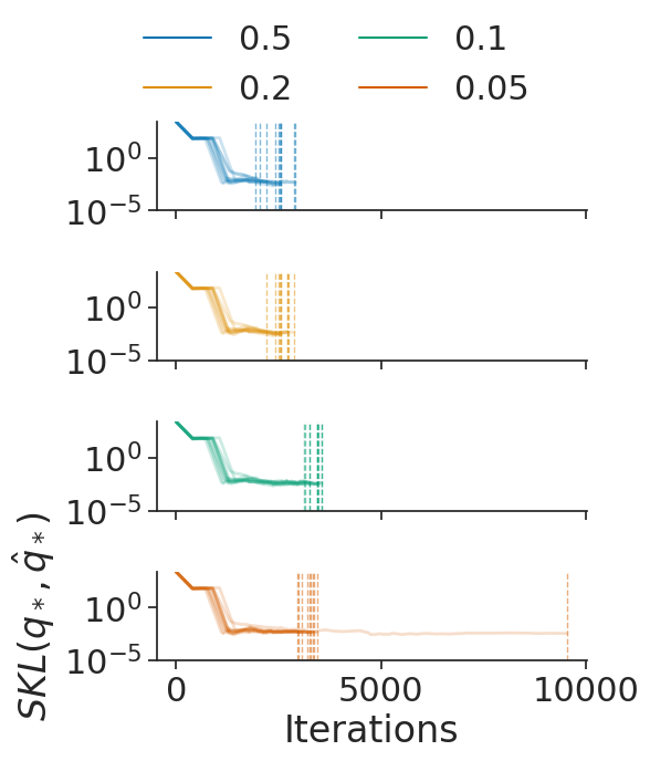
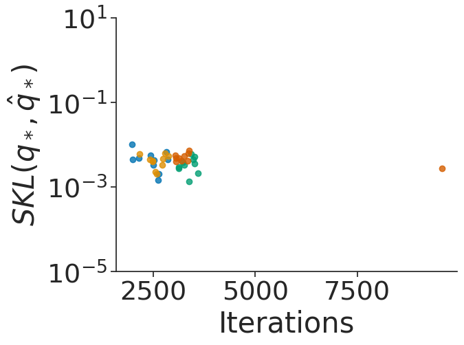
(c) $\varepsilon_{0}$

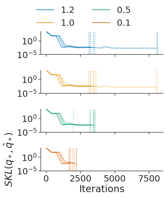
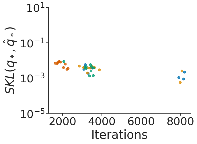
(d) $\tau$

Figure 11: Robustness to tuning parameters (a) initial learning rate $\gamma_{0}$, (b) minimum window size $W_{\min}$, (c) initial iterate average relative error threshold $\varepsilon_{0}$, and (d) inefficiency threshold $\tau$ using dogs dataset from posteriordb package. (top) Iterations versus symmetrized KL divergence between iterate average and optimal variational approximation. The transparent lines represent repeated experiments and the vertical lines indicate the termination rule trigger points. (bottom) Iterations versus symmetrized KL divergence between iterate average and optimal variational approximation at the termination rule trigger point.

8 Discussion

As we have shown through both theory and experiments, RAABBVI, our stochastic optimization framework for black-box variational inference, delivers a number of benefits compared to existing approaches:

• The user only needs to, at most, adjust a small number of tuning parameters which empower the user to intuitively control and trade off computational cost and accuracy. Moreover, RAABBVI is robust, both in terms of accuracy and computational cost, to small changes in all tuning parameters.

• Our framework can easily incorporate different stochastic optimization methods such as adaptive versions, natural gradient descent, and stochastic quasi-Newton methods. In practice we found that the averaged versions of RMSProp and Adam we propose perform particularly well. But the performance of RAABBVI will benefit from future innovations in stochastic optimization methodology.

• RAABBVI allows for any choice of tractable variational family and stochastic gradient estimator. For example, in many cases we find accuracy improves when using the full-rank Gaussian variational family rather than the mean-field one.

Our empirical results also highlight some of the limitations of BBVI, which sometimes is less accurate than dynamic HMC when given equal computational budgets. However, BBVI can be further sped up using, for example, data subsampling when the dataset size is large (which was not the case for the posteriodb datasets from our experiments).

Appendix A Proofs

A.1 Proof of Proposition 4.4

Since the KL divergence of mean-field Gaussians factors across dimensions, without loss of generality we consider the case of $\dim=1$. The symmetrized KL divergence between two Gaussians is

$$\mathrm{SKL}(\lambda_{1},\lambda_{2}) =\frac{1}{2}\left\{e^{2\psi_{1}-2\psi_{2}}+e^{2\psi_{2}-2\psi_{1}}+(\tau_{1}-\tau_{2})^{2}(e^{-2\psi_{1}}+e^{-2\psi_{2}})-2\right\}$$ (A.1)

$$=\frac{1}{2}\left\{e^{2\psi_{1}-2\psi_{2}}+e^{2\psi_{2}-2\psi_{1}}+(\tau_{1}-\tau_{2})^{2}e^{-2\psi_{1}}(1+e^{2\psi_{1}-2\psi_{2}})-2\right\}.$$ (A.2)

Recall our assumption that for some constants $A=(A_{\tau},A_{\psi})$ and $B=(B_{\tau},B_{\psi})$,

$$\bar{\lambda}_{\gamma}=\lambda_{*}+A\gamma+B\gamma^{2}+o(\gamma^{2}).$$ (A.3)

Hence

$$e^{2\bar{\psi}_{\gamma}-2\psi_{*}} =1+2A_{\psi}\gamma+2B_{\psi}\gamma^{2}+\frac{1}{2}(2A_{\psi}\gamma+2B_{\psi}\gamma^{2})^{2}+o(\gamma^{2})$$ (A.4)

$$=1+2A_{\psi}\gamma+2B_{\psi}\gamma^{2}+2A_{\psi}^{2}\gamma^{2}+o(\gamma^{2})$$ (A.5)

and similarly $e^{2\psi_{*}-2\bar{\psi}_{\gamma}}=1-2A_{\psi}\gamma-2B_{\psi}\gamma^{2}+2A_{\psi}^{2}\gamma^{2}+o(\gamma^{2})$. Therefore $e^{2\bar{\psi}_{\gamma}-2\psi_{*}}+e^{2\psi_{*}-2\bar{\psi}_{\gamma}}-2=4A_{\psi}^{2}\gamma^{2}+o(\gamma^{2})$ and $(\bar{\tau}_{\gamma}-\tau_{*})^{2}=A_{\tau}^{2}\gamma^{2}+o(\gamma^{2})$. Putting these results together, we have

$$\mathrm{SKL}(\bar{\lambda}_{\gamma},\lambda_{*}) =\frac{1}{2}\Big{[}4A_{\psi}^{2}\gamma^{2}+o(\gamma^{2})+A_{\tau}^{2}\gamma^{2}e^{-\psi_{*}}\{2-2A_{\psi}\gamma-2B_{\psi}\gamma^{2}+2\gamma^{2}A_{\psi}^{2}+o(\gamma^{2})\}\Big{]}$$ (A.6)

$$=(2A_{\psi}^{2}+A_{\tau}^{2}e^{-2\psi_{*}})\gamma^{2}+o(\gamma^{2}).$$ (A.7)

Similarly, $\mathrm{SKL}(\bar{\lambda}_{\gamma},\bar{\lambda}_{\gamma^{\prime}})=(\gamma-\gamma^{\prime})^{2}(2A_{\psi}^{2}+A_{\tau}^{2}e^{-2\psi_{*}})+o(\gamma^{2})$ as long as $\gamma^{\prime}=O(\gamma)$. In other words, letting $\bar{\lambda}_{0}:=\lambda_{*}$, we have the relation

$$\mathrm{SKL}(\bar{\lambda}_{\gamma},\bar{\lambda}_{\gamma^{\prime}})=C(\gamma-\gamma^{\prime})^{2}+o(\gamma^{2})$$ (A.8)

for some unknown constant $C$.

A.2 Proof of Proposition 4.5

If $\kappa=1$ corresponds to the statement of Proposition 4.4.

If $\kappa\in[1/2,1)$, then for some constants $\Lambda=(\Lambda_{\tau},\Lambda_{\psi})$ and $A=(A_{\tau},A_{\psi})$,

$$\bar{\lambda}_{\gamma}=\lambda_{*}+\Lambda\gamma^{\kappa}+A\gamma+o(\gamma^{2\kappa}).$$ (A.9)

Assume that $\gamma_{1}=\gamma$ and $\gamma_{2}=O(\gamma)$. For $\kappa^{\prime}>0$, let $\epsilon_{\kappa^{\prime}}:=\gamma_{1}^{\kappa^{\prime}}-\gamma_{2}^{\kappa^{\prime}}$. Then we have

$$e^{\pm 2(\bar{\psi}_{\gamma_{1}}-\bar{\psi}_{\gamma_{2}})} =1\pm 2\Lambda_{\psi}\epsilon_{\kappa}\pm 2A_{\psi}\epsilon_{1}+2(\Lambda_{\psi}^{2}\epsilon_{\kappa}^{2}+2\Lambda_{\psi}A_{\psi}\epsilon_{\kappa}\epsilon_{1}+A_{\psi}^{2}\epsilon_{1}^{2})+o(\gamma^{2\kappa}),$$ (A.10)

so

$$e^{2\bar{\psi}_{\gamma_{1}}-2\bar{\psi}_{\gamma_{2}}}+e^{2\bar{\psi}_{\gamma_{2}}-2\bar{\psi}_{\gamma_{1}}}-2 =4\Lambda_{\psi}^{2}\epsilon_{\kappa}^{2}+8\Lambda_{\psi}A_{\psi}\epsilon_{\kappa}\epsilon_{1}+4A_{\psi}^{2}\epsilon_{1}^{2}+o(\gamma^{2\kappa})$$ (A.11)

Moreover, $e^{\psi_{*}-\bar{\psi}_{\gamma_{i}}}=1+O(\gamma^{\kappa})$ and

$$(\bar{\tau}_{\gamma_{1}}-\bar{\tau}_{\gamma_{2}})^{2}=\Lambda_{\tau}^{2}\epsilon_{\kappa}^{2}+2\Lambda_{\tau}A_{\tau}\epsilon_{\kappa}\epsilon_{1}+A_{\tau}^{2}\epsilon_{1}^{2}+o(\gamma^{2\kappa}).$$ (A.12)

Putting these results together, we have

$$\begin{split}\mathrm{SKL}(\bar{\lambda}_{\gamma_{1}},\bar{\lambda}_{\gamma_{2}})&=\frac{1}{2}\Bigg{[}4\Lambda_{\psi}^{2}\epsilon_{\kappa}^{2}+8\Lambda_{\psi}A_{\psi}\epsilon_{\kappa}\epsilon_{1}+4A_{\psi}^{2}\epsilon_{1}^{2}+o(\gamma^{2\kappa})\\ &\phantom{=\frac{1}{2}\Bigg{[}}+e^{-\psi_{*}}(\Lambda_{\tau}^{2}\epsilon_{\kappa}^{\kappa}+2\Lambda_{\tau}A_{\tau}\epsilon_{\kappa}\epsilon_{1}+A_{\tau}^{2}\epsilon_{1}^{2})\{2+O(\gamma^{\kappa})\}\Bigg{]}\end{split}$$

$$=2\Lambda_{\psi}^{2}\epsilon_{\kappa}^{2}+\Lambda_{\tau}^{2}e^{-\psi_{*}}\epsilon_{\kappa}^{2}+O(\gamma^{1+\kappa})$$ (A.13)

$$=C(\gamma_{1}^{\kappa}-\gamma_{2}^{\kappa})^{2}+o(\gamma^{2\kappa}),$$ (A.14)

where $C:=2\Lambda_{\psi}^{2}+\Lambda_{\tau}^{2}e^{-\psi_{*}}$.

A.3 Symmetric KL divergence termination rule

We can use Eq. A.14 to derive a termination rule. If $\gamma$ is the current learning rate, the previous learning rate was $\gamma/\rho$. Ignoring $o(\gamma^{2\kappa})$ terms, we have

$$\delta_{\gamma}:=\mathrm{SKL}(\bar{\lambda}_{\gamma/\rho},\bar{\lambda}_{\gamma})=C\gamma^{2\kappa}(1/\rho^{\kappa}-1)^{2}.$$ (A.15)

Therefore, we can estimate $p$ and $C$ using a regression model of the form

$$\log\delta_{\gamma}=\log C+2\log(1/\rho^{\kappa}-1)+2p\log\gamma.$$ (A.16)

Given estimates $\hat{\kappa}$ and $\hat{C}$, we can estimate $\mathrm{SKL}(\bar{\lambda}_{\gamma},\lambda_{*})\approx\hat{C}\gamma^{2\hat{\kappa}}$.

A.4 Proof of Proposition 5.1

Since for $|x|<1/2$ it holds that $|\exp(x)-1|\leq 1.5|x|$, we have

$$\frac{|\hat{\sigma}_{i}-\bar{\sigma}_{i}|}{\bar{\sigma}_{i}} =|\exp(\hat{\psi}_{i}-\bar{\psi}_{i})-1|\leq 1.5\varepsilon^{\prime}$$ (A.17)

and

$$\frac{|\hat{\tau}_{i}-\bar{\tau}_{i}|}{\bar{\sigma}_{i}} \leq\varepsilon^{\prime}\hat{\sigma}_{i}/\bar{\sigma}_{i}\leq\varepsilon^{\prime}(1+1.5\varepsilon^{\prime})\leq 1.75\varepsilon^{\prime}.$$ (A.18)

A.5 Proof of Proposition 5.2

In the optimal case, the total cost for the iterations used for iterate averaging is

$$\mathrm{OPT} =C_{O}W_{\mathrm{opt}}+C_{E}W_{\mathrm{conv}}+C_{E}W_{\mathrm{opt}}$$ (A.19)

$$=C_{E}(rW_{\mathrm{opt}}+W_{\mathrm{conv}}+W_{\mathrm{opt}}).$$ (A.20)

On the other hand, if checking at window sizes $W_{j}:=\chi^{j}W_{\mathrm{conv}}\;(j=1,2,\dots)$, then window size at which convergence will be detected is $j_{*}:=\lceil\log(W_{\mathrm{opt}}/W_{\mathrm{conv}})/\log(\chi)$, and in particular

$$W_{j_{*}}\leq\chi W_{\mathrm{opt}}.$$ (A.21)

Therefore we can bound the actual computational cost as

$$C_{O}W_{j_{*}}+C_{E}W_{\mathrm{conv}}\log W_{\mathrm{conv}}+C_{E}\sum_{j=1}^{j_{*}}W_{j}$$ (A.22)

$$\leq C_{O}\chi W_{\mathrm{opt}}+C_{E}W_{\mathrm{conv}}\log W_{\mathrm{conv}}+C_{E}\sum_{j=1}^{j_{*}}\chi^{j}W_{\mathrm{conv}}$$ (A.23)

$$\leq C_{O}\chi W_{\mathrm{opt}}+C_{E}W_{\mathrm{conv}}\log W_{\mathrm{conv}}+C_{E}\frac{\chi(\chi^{j_{*}}-1)W_{\mathrm{conv}}}{\chi-1}$$ (A.24)

$$\leq C_{O}\chi W_{\mathrm{opt}}+C_{E}W_{\mathrm{conv}}\log W_{\mathrm{conv}}+C_{E}\frac{\chi^{2}W_{\mathrm{opt}}}{\chi-1}$$ (A.25)

$$=C_{E}\left[\chi rW_{\mathrm{opt}}+W_{\mathrm{conv}}+\frac{\chi^{2}}{\chi-1}W_{\mathrm{opt}}\right].$$ (A.26)

If $\chi=2$, then the actual computational cost is bounded by

$${C_{E}\left[2rW_{\mathrm{opt}}+W_{\mathrm{conv}}+4W_{\mathrm{opt}}\right]} \leq 4C_{E}\left[rW_{\mathrm{opt}}+W_{\mathrm{conv}}+W_{\mathrm{opt}}\right]$$ (A.27)

$$=4\,\mathrm{OPT}.$$ (A.28)

On the other hand, we can minimize the total cost by solving $\chi_{*}:=\operatornamewithlimits{arg\,min}_{\chi>1}\{r\chi+\chi^{2}/(\chi-1)\}=\chi(r)$. Plugging this back in, we get the bound

$$C_{E}\frac{2+r+2\mathchoice{{\hbox{$\displaystyle\sqrt{1+r\,}$}\lower 0.4pt\hbox{\vrule height=6.44444pt,depth=-5.15558pt}}}{{\hbox{$\textstyle\sqrt{1+r\,}$}\lower 0.4pt\hbox{\vrule height=6.44444pt,depth=-5.15558pt}}}{{\hbox{$\scriptstyle\sqrt{1+r\,}$}\lower 0.4pt\hbox{\vrule height=4.51111pt,depth=-3.6089pt}}}{{\hbox{$\scriptscriptstyle\sqrt{1+r\,}$}\lower 0.4pt\hbox{\vrule height=3.22221pt,depth=-2.57779pt}}}}{1+r}\left(rW_{\mathrm{opt}}+W_{\mathrm{conv}}\log W_{\mathrm{conv}}+W_{\mathrm{opt}}\right)$$ (A.29)

$$=\frac{2+r+2\mathchoice{{\hbox{$\displaystyle\sqrt{1+r\,}$}\lower 0.4pt\hbox{\vrule height=6.44444pt,depth=-5.15558pt}}}{{\hbox{$\textstyle\sqrt{1+r\,}$}\lower 0.4pt\hbox{\vrule height=6.44444pt,depth=-5.15558pt}}}{{\hbox{$\scriptstyle\sqrt{1+r\,}$}\lower 0.4pt\hbox{\vrule height=4.51111pt,depth=-3.6089pt}}}{{\hbox{$\scriptscriptstyle\sqrt{1+r\,}$}\lower 0.4pt\hbox{\vrule height=3.22221pt,depth=-2.57779pt}}}}{1+r}\mathrm{OPT}$$ (A.30)

$$<4\,\mathrm{OPT}.$$ (A.31)

Appendix B Further Details

B.1 Effective sample size (ESS) and Monte Carlo standard error (MCSE)

Let $v^{(1)},v^{(2)},\dots$ denote a stationary Markov chain, let $\bar{v}:=\mathbb{E}[v^{(1)}]$ denote the mean at stationarity, and let $\hat{v}:=K^{-1}\sum_{k=1}^{K}v^{(k)}$ denote the Monte Carlo estimate for $\bar{v}$. The (ideal) effective sample size is defined as

$$\mathrm{ESS}(K):=K/(1+\sum_{k=1}^{\infty}\rho_{k}),$$ (B.1)

where $\rho_{k}$ is the autocorrelation of the Markov chain at lag $k$. The ESS can be efficiently estimated using a variety of methods [24, 58]. We write $\widehat{\mathrm{ESS}}(v^{(1:K)})$ to denote an estimator for $\mathrm{ESS}(K)$ based on the sequence $v^{(1:K)}:=(v^{(1)},\dots,v^{(K)})$. The Monte Carlo standard error of $\hat{v}$ is given by

$$MCSE(\hat{v}):=\sigma(v^{(1)})/\mathrm{ESS}(K),$$ (B.2)

where $\sigma(v^{(1)})$ denote the standard deviation of the random variable $v^{(1)}$. Given the empirical standard deviation of $v^{(1)},\dots,v^{(K)}$, which we denote $\hat{\sigma}(v^{(1:K)})$, the MCSE can be approximated by

$$\widehat{\mathrm{MCSE}}(v^{(1:K)}):=\hat{\sigma}(v^{(1:K)})/\widehat{\mathrm{ESS}}(v^{(1:K)}).$$ (B.3)

B.2 Total variation distance and KL divergence

For distributions $\eta$ and $\zeta$, $|I_{\eta,i,a,b}-I_{\zeta,i,a,b}|\leq\mathchoice{{\hbox{$\displaystyle\sqrt{\mathrm{KL}(\eta\mid\zeta)/2\,}$}\lower 0.4pt\hbox{\vrule height=7.5pt,depth=-6.00003pt}}}{{\hbox{$\textstyle\sqrt{\mathrm{KL}(\eta\mid\zeta)/2\,}$}\lower 0.4pt\hbox{\vrule height=7.5pt,depth=-6.00003pt}}}{{\hbox{$\scriptstyle\sqrt{\mathrm{KL}(\eta\mid\zeta)/2\,}$}\lower 0.4pt\hbox{\vrule height=5.25pt,depth=-4.20003pt}}}{{\hbox{$\scriptscriptstyle\sqrt{\mathrm{KL}(\eta\mid\zeta)/2\,}$}\lower 0.4pt\hbox{\vrule height=3.75pt,depth=-3.00002pt}}}$ for all $a<b$ and $i$. This guarantee follows from Pinsker’s inequality, which relates the KL divergence to the total variation distance

$$d_{\mathrm{TV}}(\eta,\zeta):=\sup_{f:\left\|{f}\right\|_{\infty}\leq 1}\left|\int f(\theta)\eta(\mathrm{d}\theta)-\int f(\theta)\zeta(\mathrm{d}\theta)\right|,$$ (B.4)

where $\left\|{f}\right\|_{\infty}:=\sup_{\theta}f(\theta)-\inf_{\theta}f(\theta)$. Specifically, Pinsker’s inequality states that $d_{\mathrm{TV}}(\eta,\zeta)\leq\mathchoice{{\hbox{$\displaystyle\sqrt{\mathrm{KL}(\eta\mid\zeta)/2\,}$}\lower 0.4pt\hbox{\vrule height=7.5pt,depth=-6.00003pt}}}{{\hbox{$\textstyle\sqrt{\mathrm{KL}(\eta\mid\zeta)/2\,}$}\lower 0.4pt\hbox{\vrule height=7.5pt,depth=-6.00003pt}}}{{\hbox{$\scriptstyle\sqrt{\mathrm{KL}(\eta\mid\zeta)/2\,}$}\lower 0.4pt\hbox{\vrule height=5.25pt,depth=-4.20003pt}}}{{\hbox{$\scriptscriptstyle\sqrt{\mathrm{KL}(\eta\mid\zeta)/2\,}$}\lower 0.4pt\hbox{\vrule height=3.75pt,depth=-3.00002pt}}}$. Thus, small KL divergence implies small total variance distance, which implies the difference between expectations for any function $f$ such that $\left\|{f}\right\|_{\infty}$ is small. In the case of interval probabilities, since $\left\|{\mathds{1}(\cdot\in[a,b])}\right\|_{\infty}=1$, it follows that

$$|I_{\eta,i,a,b}-I_{\zeta,i,a,b}| =\left|\int\mathds{1}(\theta\in[a,b])\eta(\mathrm{d}\theta)-\int\mathds{1}(\theta\in[a,b])\zeta(\mathrm{d}\theta)\right|$$ (B.5)

$$\leq\left\|{\mathds{1}(\cdot\in[a,b])}\right\|_{\infty}d_{\mathrm{TV}}(\eta,\zeta)$$ (B.6)

$$\leq\mathchoice{{\hbox{$\displaystyle\sqrt{\mathrm{KL}(\eta\mid\zeta)/2\,}$}\lower 0.4pt\hbox{\vrule height=7.5pt,depth=-6.00003pt}}}{{\hbox{$\textstyle\sqrt{\mathrm{KL}(\eta\mid\zeta)/2\,}$}\lower 0.4pt\hbox{\vrule height=7.5pt,depth=-6.00003pt}}}{{\hbox{$\scriptstyle\sqrt{\mathrm{KL}(\eta\mid\zeta)/2\,}$}\lower 0.4pt\hbox{\vrule height=5.25pt,depth=-4.20003pt}}}{{\hbox{$\scriptscriptstyle\sqrt{\mathrm{KL}(\eta\mid\zeta)/2\,}$}\lower 0.4pt\hbox{\vrule height=3.75pt,depth=-3.00002pt}}}.$$ (B.7)

B.3 Adaptive SASA+

The SASA+ algorithm of Zhang et al. [66] generalizes the approach of Yaida [64]. The main idea is to find an appropriate invariant function $\Delta(d,\lambda)$ that satisfies $\int\Delta(d,\lambda)\mu_{\gamma}(\mathrm{d}d,\mathrm{d}\lambda)=0$. Yaida [64] derived valid forms of $\Delta$ for specific choices of the descent direction, while Zhang et al. [66] showed that for any optimizer of the form Eq. 4 that is time-homogenous with $\gamma^{(k)}=\gamma$, the map $(d,\lambda)\mapsto 2\langle{d},{\lambda}\rangle-\gamma\left\|{d}\right\|^{2}$ is a valid invariant function. The SASA+ algorithm proposed by Zhang et al. [66] uses a hypothesis test to determining when the iterates are sufficiently close to stationarity. Let $\Delta^{(k)}:=2\langle{d^{(k)}},{\lambda^{(k)}}\rangle-\gamma\left\|{d^{(k)}}\right\|^{2}$ and let $W=\lceil\varrho k\rceil$ denote the window size to use for checking stationarity. Once $W$ is at least equal to a minimum window size $W_{\min}$, SASA+ uses $\Delta^{(k-W+1)},\dots,\Delta^{(k)}$ to carry out a hypothesis test, where the null hypothesis is that $\mathbb{E}[\Delta^{(k)}]=0$.

We make several adjustments to reduce the number of tuning parameters and to make the remaining ones more intuitive. Note that the SASA+ convergence criterion requires the choice of three parameters: $\varrho$, $W_{\min}$, and the size of the hypothesis test $\alpha$. Zhang et al. [66] showed empirically and our numerical experiments confirmed that the choice of $\alpha$ has little effect and therefore does not need to be adjusted by the user. The choices for $\varrho$ and $W_{\min}$, however, have a substantial effect on efficiency. If $\varrho$ is too big, then early iterations that are not at stationarity will be included, preventing the detection of convergence. On the other hand, if $\varrho$ is too small, then the total number of iterations must be large (specifically, greater than $W_{\min}/\varrho$) before the window size is large enough to trigger the first check for stationarity. Moreover, the correct choice of $W_{\min}$ will vary depending on the problem. If the iterates have large autocorrelation then $W_{\min}$ should be large, while if the autocorrelation is small or negative, then $W_{\min}$ can be small.

Our approach to determining the optimal window size instead relies on the effective sample size (ESS). $W_{\mathrm{opt}}$ that maximizes $\widehat{\mathrm{ESS}}(W):=\widehat{\mathrm{ESS}}(\Delta^{(k-W+1)},\dots,\Delta^{(k)})$, where $k$ is the current iteration. To ensure reliability, we impose additional conditions on $W_{\mathrm{opt}}$. First, we require that $\widehat{\mathrm{ESS}}(W_{\mathrm{opt}})\geq N_{\min}$, a user-specified minimum effective sample size. Unlike $W_{\min}$, $N_{\min}$ has an intuitive and direct interpretation. The second condition is, when finding $W_{\mathrm{opt}}$, the search over values of $W$ is constrained to the lower bound of $N_{\min}$ (to ensure the estimator is sufficiently reliable) and the upper bound of $0.95k$ (to always allow for some “burn-in”). In practice we do not check all $W\in\{N_{\min},\dots,0.95k\}$, but rather perform a grid search over 5 equally spaced values ranging from $N_{\min}$ to $0.95k$.

A slightly different version which may improve power is to instead define the multivariate invariant function $\vec{\Delta}(d,\lambda)=2d\odot\lambda-d\odot d$, where we recall that $\odot$ denotes component-wise multiplication. In this case a multivariate hypothesis test such as Hotelling’s $T^{2}$ test or the multivariate sign test, where a single effective sample size (e.g., the median component-wise ESS) could be used. Alternatively, a separate hypothesis test for each of the $m$ components could be used, with stationarity declared once all tests confirm stationarity (using, e.g., a test size of $\alpha/m$). While this approach might be more computationally efficient when $m$ is large, it could come at the cost of test power.

B.4 Distance Based Convergence Detection

Pesme, Dieuleveut and Flammarion [45] proposed a distance based diagnostic algorithm to detect the stationarity of the SGD optimization algorithm. The main idea behind this algorithm is to find the distance between the current iterate $\lambda_{k}$ and the optimal variational parameter $\lambda_{*}$, $\left\|{\eta_{k}}\right\|:=\left\|{\lambda_{k}-\lambda_{*}}\right\|$. Since optimal variational parameter $\lambda_{*}$ unknown, this distance cannot be directly observed. Therefore, they suggested using the distance between the current iterate $\lambda_{k}$ and the initial iterate of the current learning rate, $\left\|{\Omega_{k}}\right\|:=\left\|{\lambda_{k}-\lambda_{0}}\right\|$ and showed that $\left\|{\eta_{k}}\right\|$ and $\left\|{\Omega_{k}}\right\|$ have a similar behavior.

Under the setting of quadratic objective function with additive noise, they computed the behavior of the expectation of $\left\|{\Omega_{k}}\right\|^{2}$ in closed-form to detect the convergence of $\left\|{\lambda_{k}-\lambda_{0}}\right\|^{2}$. With the result, they have shown the asymptotic behavior of the $\mathbb{E}[\left\|{\Omega_{k}}\right\|^{2}]$ in the transient and stationary phases, where $\mathbb{E}[\left\|{\Omega_{k}}\right\|^{2}]$ has a slope greater than $1$ and slope of $0$ in a log-log plot respectively. Hence, the slope $S:=\frac{\log\left\|{\lambda_{k}-\lambda_{0}}\right\|^{2}-\log\left\|{\lambda_{k}/q-\lambda_{0}}\right\|^{2}}{\log k-\log k/q}$ computed between iterations $q^{n}$ and $q^{n+1}$ for $q>1$ and $n\geq n_{0}$ where $n_{0}\in\mathcal{N}^{*}$ and if $S<\mathrm{thresh}$ ($\mathrm{thresh}\in(0,2]$) then the convergence will be detected.

B.5 Stochastic Quasi-Newton Optimization

The algorithm of Liu and Owen [37] provide a randomized approach of classical quasi-Newton (QN) method that is known as stochastic quasi-Newton (SQN) method. Even though, Liu and Owen [37] use randomized quasi-Monte Carlo (RMCQ) samples we use Monte Carlo (MC) samples to compute the gradient . In classical quasi-Newton optimization the Newton update is

$$\lambda^{(k+1)}\leftarrow\lambda^{(k)}-(\nabla^{2}_{\lambda^{(k)}}D_{\pi}(q_{\lambda^{(k)}}))^{-1}\nabla_{\lambda^{(k)}}D_{\pi}(q_{\lambda^{(k)}}),$$ (B.8)

where $\nabla^{2}_{\lambda^{(k)}}D_{\pi}(q_{\lambda^{(k)}})$ is the Hessian matrix of $D_{\pi}(q_{\lambda^{(k)}})$. However, computation cost of Hessian matrix and its inverse is high and it also takes a large space. Therefore, we can use BFGS (discovered by Broyden, Fletcher, Goldfarb, and Shanno) method where it approximate the inverse of $\nabla^{2}_{\lambda^{(k)}}D_{\pi}(q_{\lambda^{(k)}})$ using $H_{k}$ at the $k$th iteration by initializing it with an identity matrix. Then the update is modified by

$$\lambda^{(k+1)}\leftarrow\lambda^{(k)}-\gamma^{(k)}H^{(k)}\nabla_{\lambda^{(k)}}D_{\pi}(q_{\lambda^{(k)}}),$$ (B.9)

where

$$H^{(k+1)}\leftarrow\Big{(}I-\frac{s_{k}y^{T}_{k}}{s^{T}_{k}y_{k}}\Big{)}H^{(k)}\Big{(}I-\frac{y_{k}s^{T}_{k}}{s^{T}_{k}y_{k}}\Big{)}+\frac{s_{k}s^{T}_{k}}{s^{T}_{k}y_{k}},$$ (B.10)

$s_{k}=\lambda^{(k+1)}-\lambda^{(k)}$, and $y_{k}=\nabla_{\lambda^{(k+1)}}D_{\pi}(q_{\lambda^{(k+1)}})-\nabla_{\lambda^{(k)}}D_{\pi}(q_{\lambda^{(k)}})$. Even using the above Hessian approximation $H^{(k)}$ will require large space for storage. To over come that problem we can use Limited-memory BFGS (L-BFGS) [43] that computes $H^{(k)}\nabla_{\lambda^{(k)}}D_{\pi}(q_{\lambda^{(k)}})$ using $m$ most recent $(s_{k},y_{k})$ correction pairs. Liu and Owen [37] use the stochastic quasi-Newton approach proposed by Chen et al. [11] and they compute the correction pairs after every $B$ iterations by computing the iterate average of parameters using the most recent $B$ iterations. To compute the $y_{k}$, the gradients of the objective function is estimated by using MC samples that is independent from the MC samples obtained to compute the gradient in the update step.

B.6 Natural Gradient Descent Optimization

Khan and Lin [31] proposed natural gradient descent (NGD) approach for variational inference that utilize the information geometry of the variational distribution. Given the variational distribution is a exponential family distribution

$$q_{\lambda}=h\exp(\phi^{T}\lambda-A(\lambda))$$ (B.11)

the NGD update is

$$\lambda^{(k+1)}\leftarrow\lambda^{(k)}-\gamma^{(k)}(F(\lambda^{(k)}))^{-1}\nabla_{\lambda^{(k)}}D_{\pi}(q_{\lambda^{(k)}}),$$ (B.12)

where $F(\lambda^{(k)})$ denote the Fisher Information Matrix (FIM) of the distribution and $\lambda$ denote its natural-parameter. Without directly computing the inverse of FIM Khan and Lin [31] simplified the above update by using the relationship between natural parameter $\lambda$ and expectation parameter $m=\mathrm{E}_{q}[\phi]$ of the exponential family

$$F(\lambda)^{-1}\nabla_{\lambda}D_{\pi}(q_{\lambda})=\nabla_{m}D_{\pi}(q_{m}).$$ (B.13)

Therefore, the natural-gradient update can be simplified as

$$\lambda^{(k+1)}\leftarrow\lambda^{(k)}-\gamma^{(k)}\nabla_{m^{(k)}}D_{\pi}(q_{m^{(k)}}).$$ (B.14)

This can be applied for the mean-field Gaussian variational family $q=\prod_{i=1}^{d}\mathcal{N}(\mu_{i},\sigma^{2}_{i})$ where we can define the natural parameters $\lambda_{i}=(\mu_{i}/\sigma^{2}_{i},-0.5/\sigma^{2}_{i})$ and expectation parameters $m=(\mu_{i},\mu_{i}^{2}+\sigma^{2}_{i})$.

Appendix C Additional Experimental Details and Results

Table C.1: Datasets of PosteriorDB Package

Dataset	Short Name	Dimensions	Model Description
arK-arK	arK	7	AR(5) time series
bball_drive_event_0-hmm_drive_0	bball_0	8	Hidden Markov model
bball_drive_event_1-hmm_drive_1	bball_1	8	Hidden Markov model
diamonds-diamonds	diamonds	26	Log-Log
dogs-dogs	dogs	3	Logistic mixed-effects
dogs-dogs_log	dogs_log	2	Logarithmic mixed-effects
earnings-logearn_interaction	earnings	5	Log-linear
eight_schools-eight_schools_noncentered	8schools_nc	10	Non-centered hierarchical
eight_schools-eight_schools_centered	8schools_c	10	Centered hierarchical
garch-garch11	garch	4	GARCH(1,1) time series
gp_pois_regr-gp_pois_regr	gp_pois_regr	13	Gaussian process Poisson regression
gp_pois_regr-gp_regr	gp_regr	3	Gaussian process regression
hmm_example-hmm_example	hmm_example	6	Hidden Markov model
hudson_lynx-hare_lotka_volterra	hudson_lynx	8	Lotka-Volterra error
low_dim_gauss_mix-low_dim_gauss_mix	low_dim_gauss_mix	5	Two-dimensional Gaussian mixture
mcycle_gp-accel_gp	mcycle_gp	66	Gaussian process
nes2000-nes	nes2000	10	Multiple predictor linear
sblrc-blr	sblrc	6	Linear

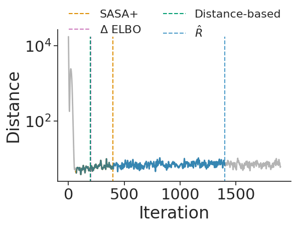
(a) uncorrelated $d=100$

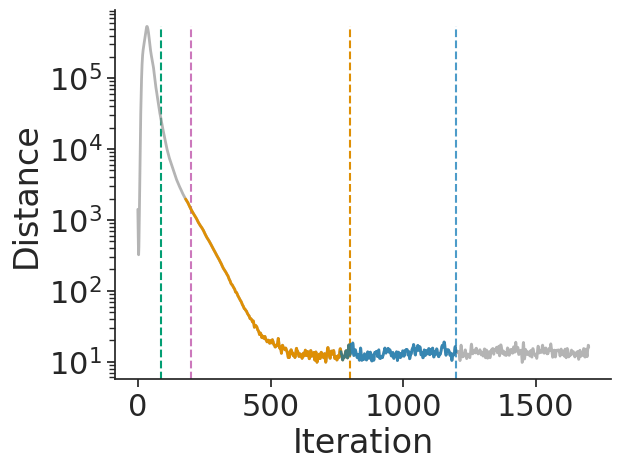
(b) uniform correlated $d=100$

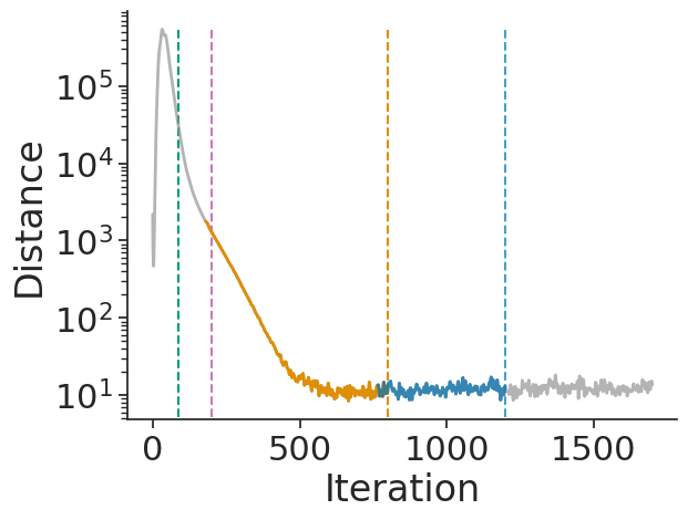
(c) banded correlated $d=100$

Figure C.1: Iteration number versus distance between iterate average and current iterate. The vertical lines indicate convergence detection trigger points and (for SASA+ and $\widehat{R}$) the colored portion of the accuracy values indicate they are part of the window used for convergence detection.

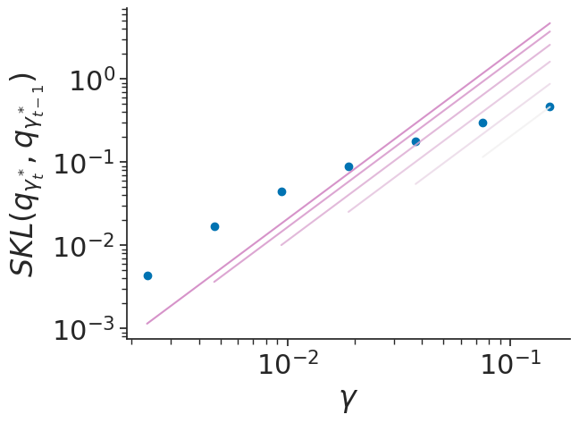
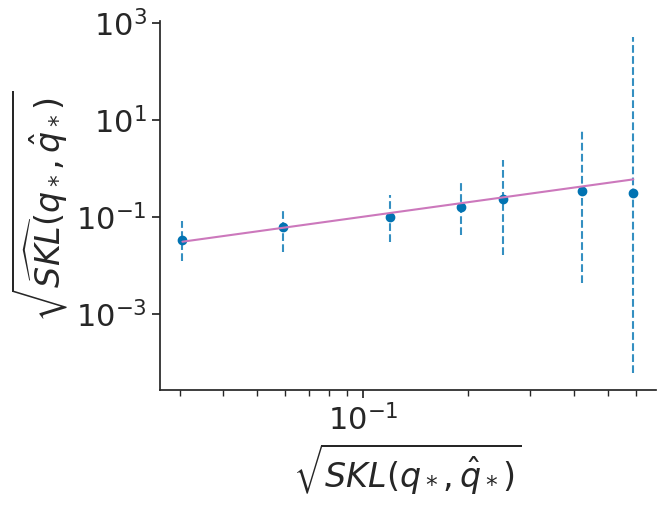
(a) uncorrelated $d=500$

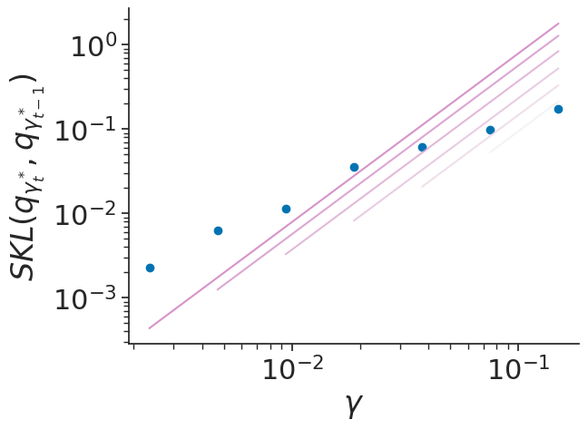
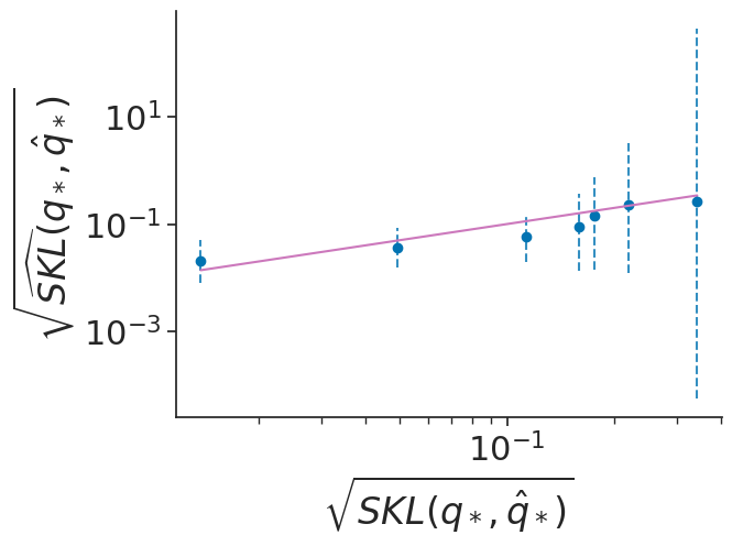
(b) uniform correlated $d=100$

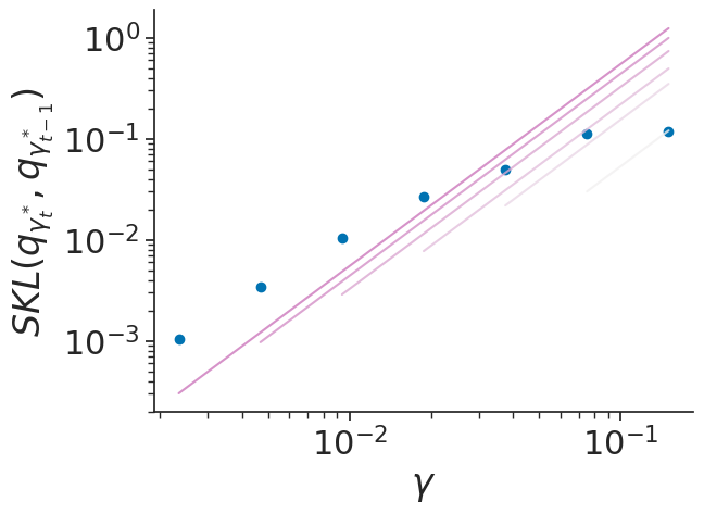
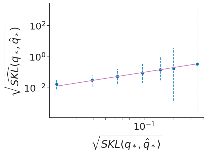
(c) banded correlated $d=100$

Figure C.2: Results for estimating the symmetrized KL divergence with avgAdam. (left) Learning rate versus symmetrized KL divergence of adjacent iterate averaged estimates of optimal variational distribution. The lines indicate the linear regression fits, with setting $\kappa=1$. (right) Square root of true symmetrized KL divergence versus the estimated value with $95\%$ credible interval. The uncertainty of the estimates decreases and remains well-calibrated as the learning rate decreases.

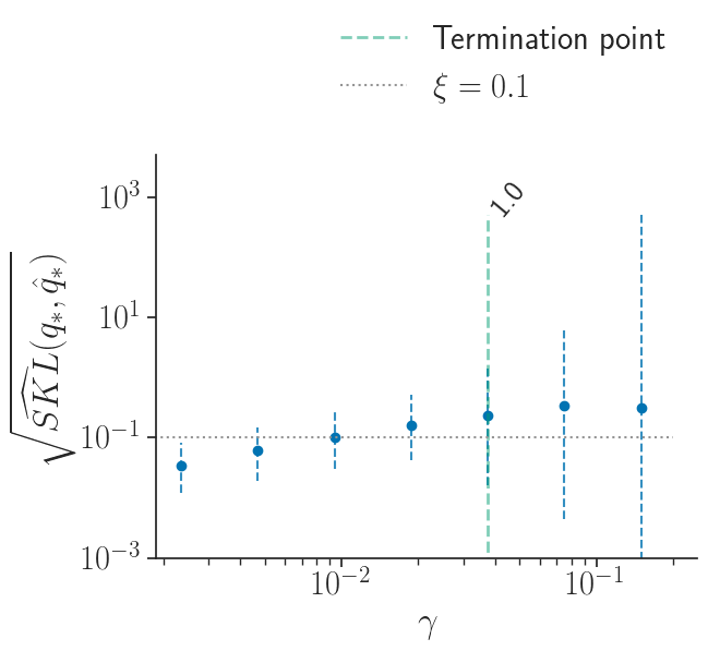
(a) uncorrelated $d=500$

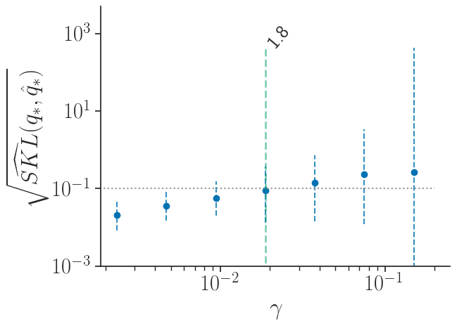
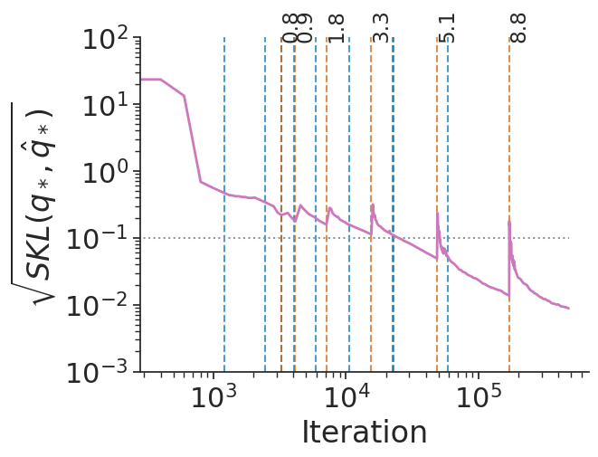
(b) uniform correlated $d=100$

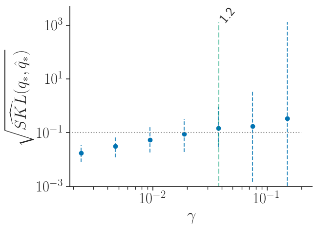
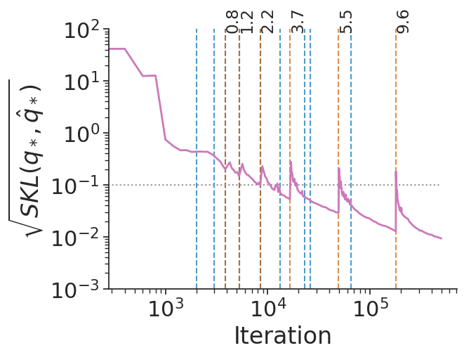
(c) banded correlated $d=100$

Figure C.3: Results of termination rule trigger point of Gaussian targets. (left) Learning rate versus square root of estimated symmetrized KL divergence with 95% credible interval (dashed blue line). The green vertical line indicates the termination rule trigger point with corresponding $\hat{\mathcal{I}}$ value. (right) Iterations versus square root of symmetrized KL divergence between iterate average and optimal variational approximation. The vertical lines indicate the convergence detection points using $\hat{R}$ (blue) and inefficiency index computation ($\hat{\mathcal{I}}$) points (orange) with corresponding values.

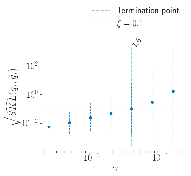
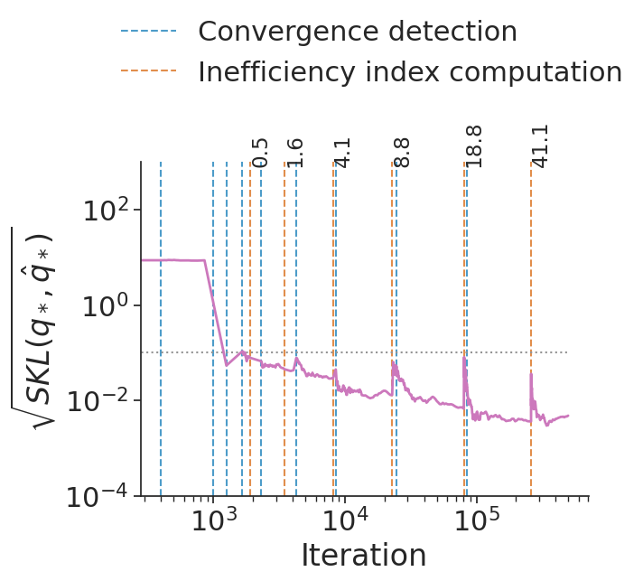
(a) dogs

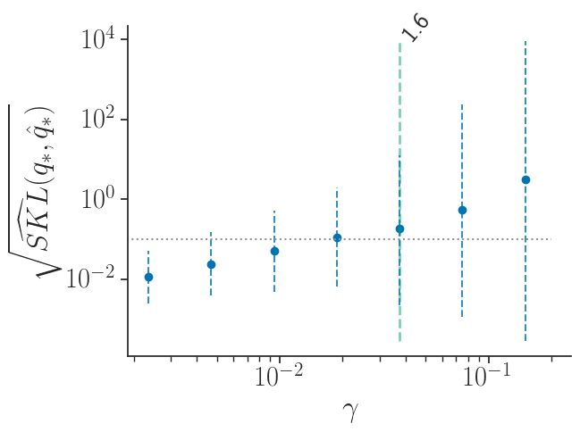
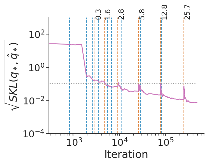
(b) arK

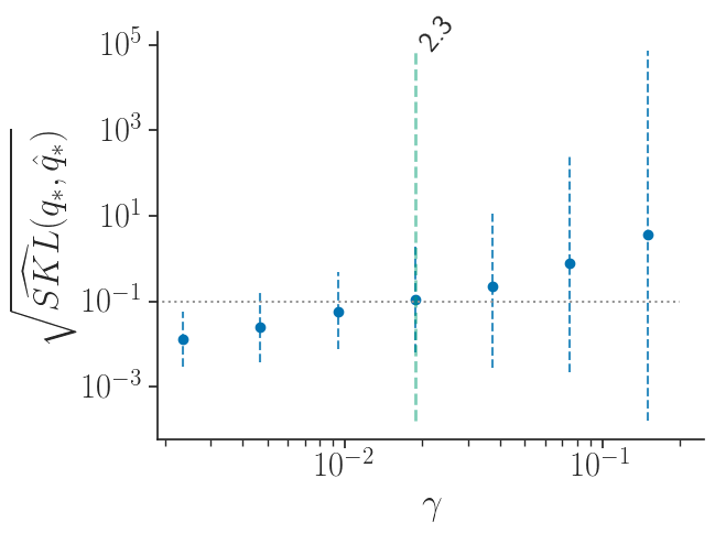
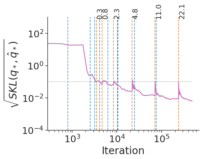
(c) nes2000

Figure C.4: Results of termination rule trigger point of posteriordb package datasets. (left) Learning rate versus square root of estimated symmetrized KL divergence with 95% credible interval (dashed blue line). The green vertical line indicates the termination rule trigger point with corresponding $\hat{\mathcal{I}}$ value. (right) Iterations versus square root of symmetrized KL divergence between iterate average and optimal variational approximation. The vertical lines indicate the convergence detection points using $\hat{R}$ (blue) and inefficiency index computation ($\hat{\mathcal{I}}$) points (orange) with corresponding values.

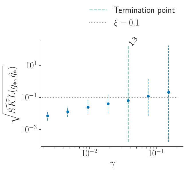
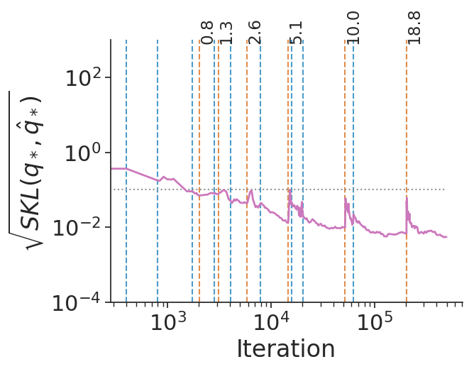
(a) 8schools_nc

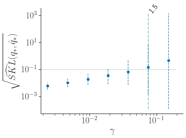
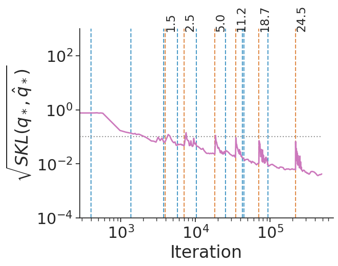
(b) 8schools_c

Figure C.5: Results of termination rule trigger point of posteriordb package datasets. (left) Learning rate versus square root of estimated symmetrized KL divergence with 95% credible interval (dashed blue line). The green vertical line indicates the termination rule trigger point with corresponding $\hat{\mathcal{I}}$ value. (right) Iterations versus square root of symmetrized KL divergence between iterate average and optimal variational approximation. The vertical lines indicate the convergence detection points using $\hat{R}$ (blue) and inefficiency index computation ($\hat{\mathcal{I}}$) points (orange) with corresponding values.

(a) uncorrelated $d=100$

(b) uncorrelated $d=500$

(c) uniform correlated $d=100$

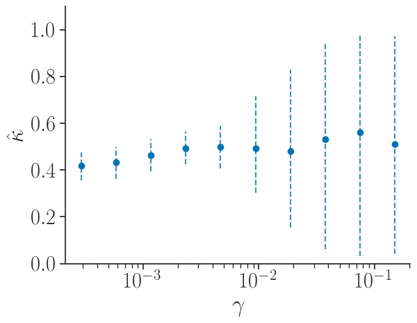
(d) banded correlated $d=100$

Figure C.6: Learning rate versus $\hat{\kappa}$ for Gaussian targets using adaptive SGD optimization (RMSProp) with 95% credible interval. The $\hat{\kappa}$ approximately reach to $0.5$ at the final learning rate in all scenrios.

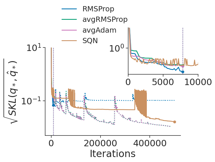
(a) uncorrelated $d=100$

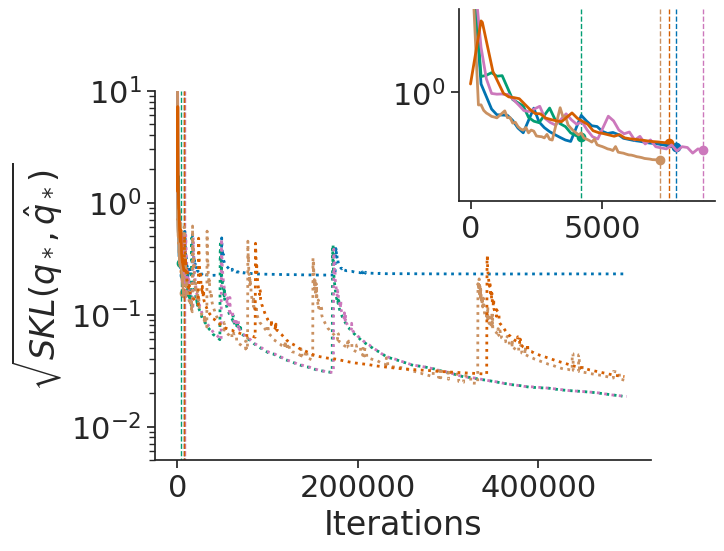
(b) uncorrelated $d=500$

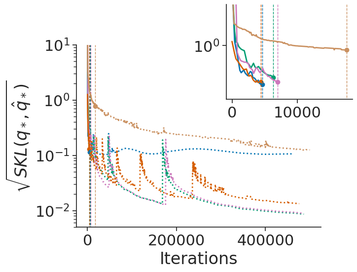
(c) uniform correlated $d=100$

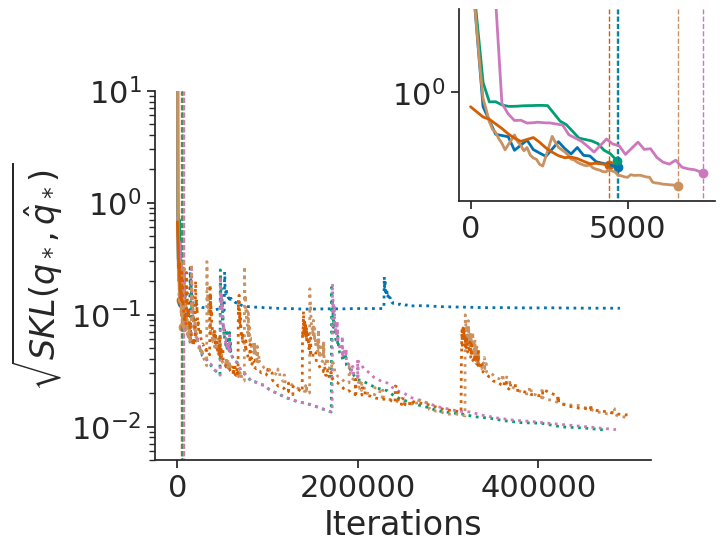
(d) banded correlated $d=100$

Figure C.7: Accuracy comparison of RMSProp, avgRMSProp, avgAdam, SQN, and NGD optimization methods in RAABBVI using Gaussian targets where accuracy is measured in terms of square root of symmetrized KL divergence between iterate average and optimal variational approximation. ($\star$) The vertical lines indicate the termination rule trigger points and the behavior of optimization methods at the trigger points showed in zoom-in plots.

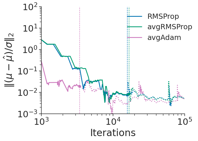
(a) dogs

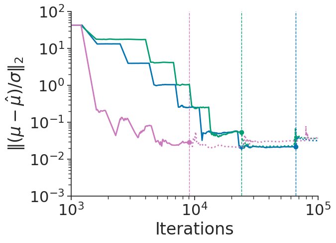
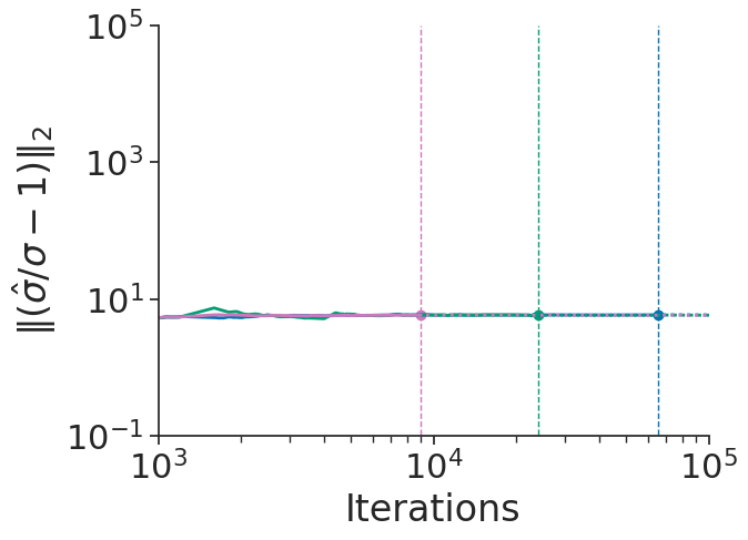
(b) arK

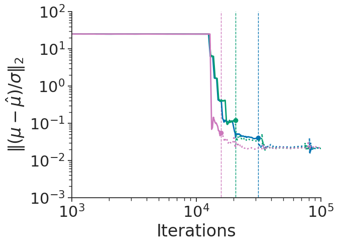
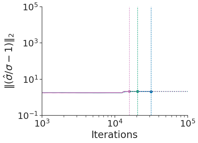
(c) nes2000

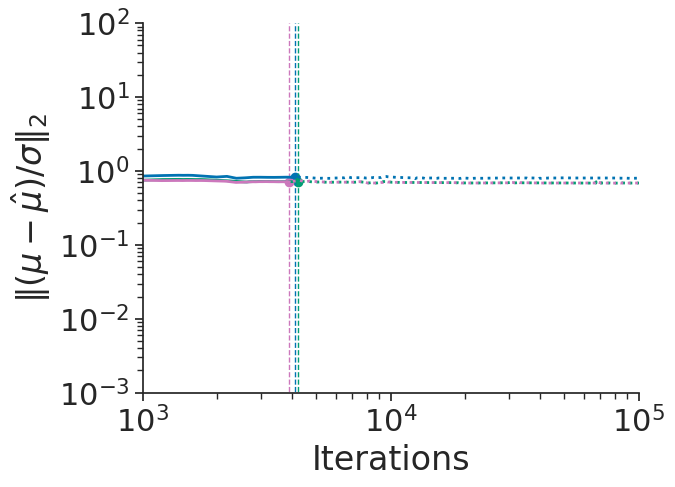
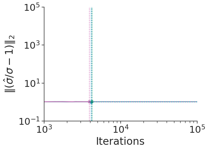
(d) 8schools_c

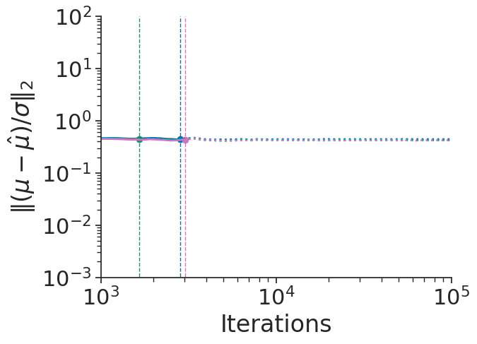
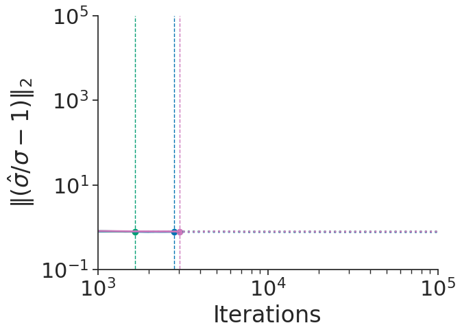
(e) 8schools_nc

Figure C.8: Accuracy comparison of RMSProp, avgRMSProp, and avgAdam optimization methods in RAABBVI using posteriordb datasets, where accuracy measured in terms of relative mean error (top) and relative standard deviation error (bottom). The vertical lines indicate the termination rule trigger points.

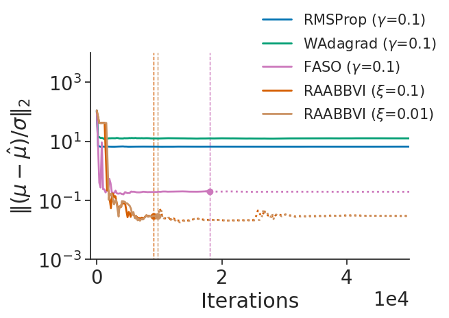
(a) arK

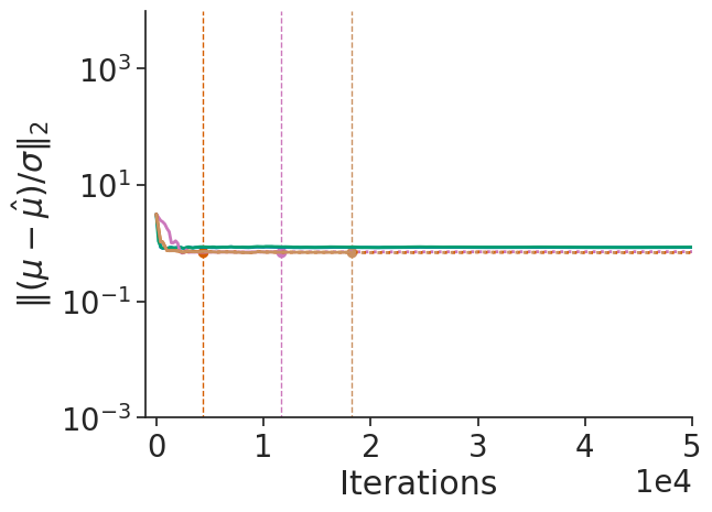
(b) 8schools_c

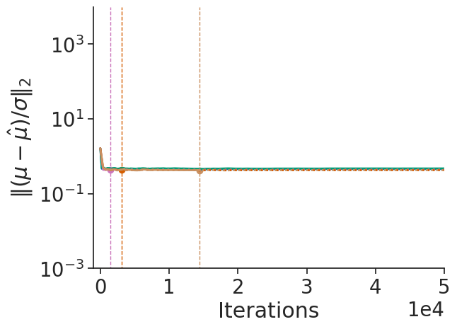
(c) 8schools_nc

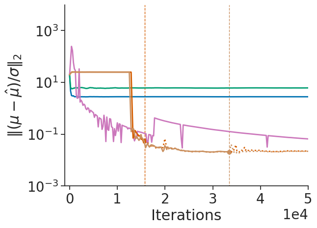
(d) nes2000

Figure C.9: Accuracy comparison of variational inference algorithms using posteriordb models and datasets, where accuracy is measure in terms of relative mean error. The vertical lines indicate the termination rule trigger points of FASO and RAABBVI. Iterate average for RMSProp and WAdagrad computed at every $200^{th}$ iteration using a window size of 20% of iterations.

(a) arK

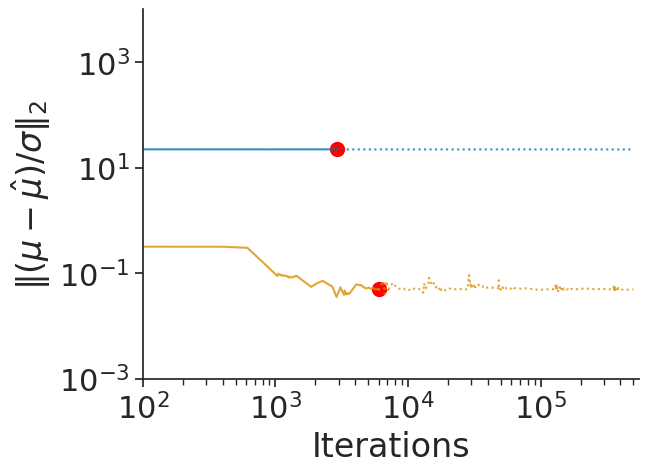
(b) bball_0

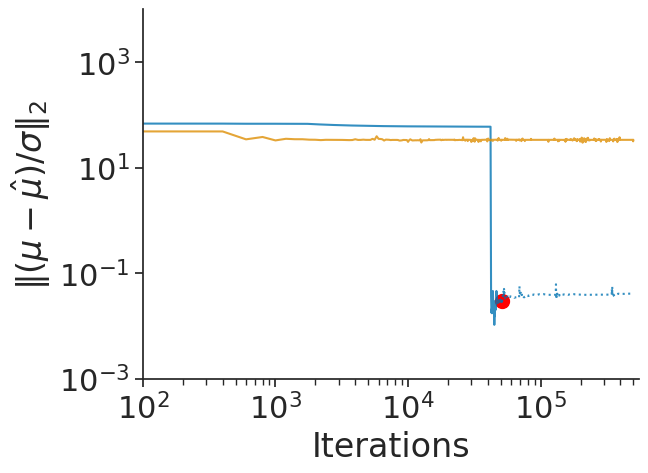
(c) bball_1

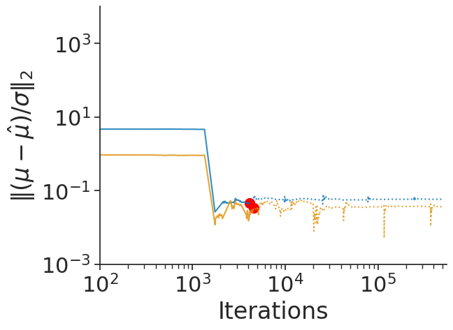
(d) dogs_log

(e) dogs

(f) diamonds

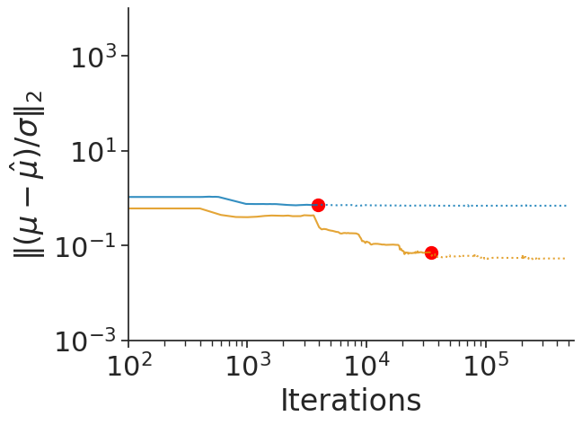
(g) 8schools_c

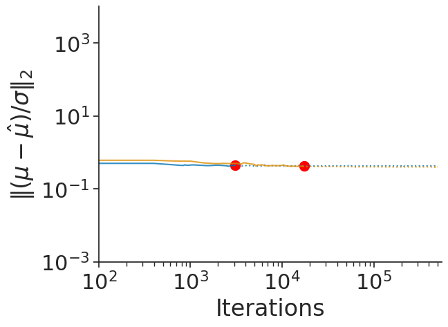
(h) 8schools_nc

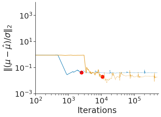
(i) hmm_example

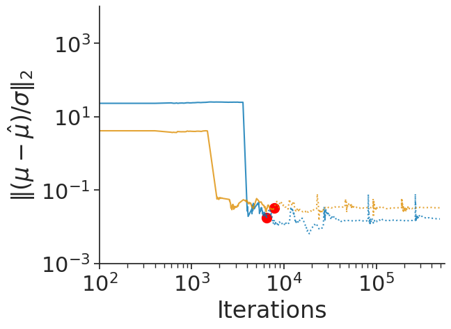
(j) low_dim_gauss

(k) nes2000

(l) sblrc

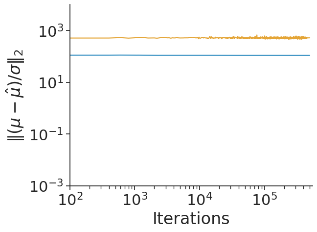
(m) earnings

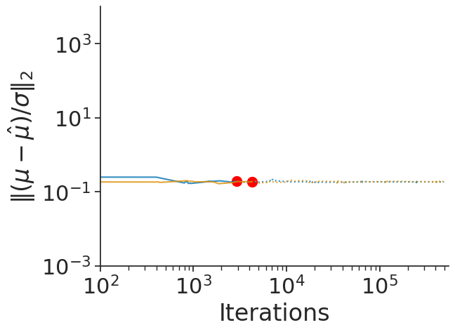
(n) garch

(o) gp_pois_regr

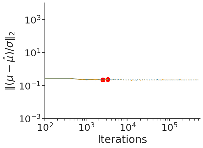
(p) gp_regr

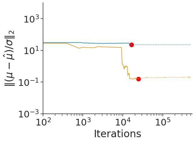
(q) hudson_lynx

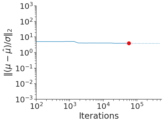
(r) mcycle_gp

Figure C.10: Accuracy of mean-field (blue) and full-rank (orange) Gaussian family approximations for selected posteriordb data/models, where accuracy is measured in terms of relative mean error. The red dots indicate where the termination rule triggers

(a) arK

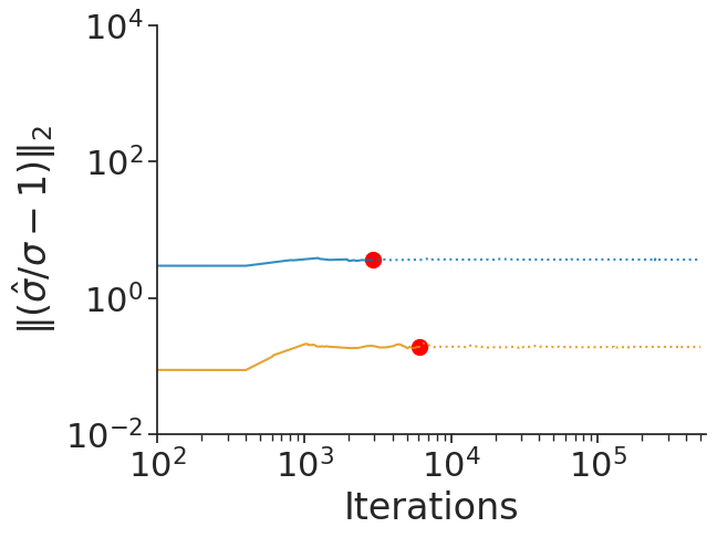
(b) bball_0

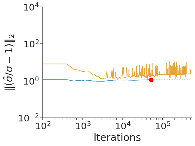
(c) bball_1

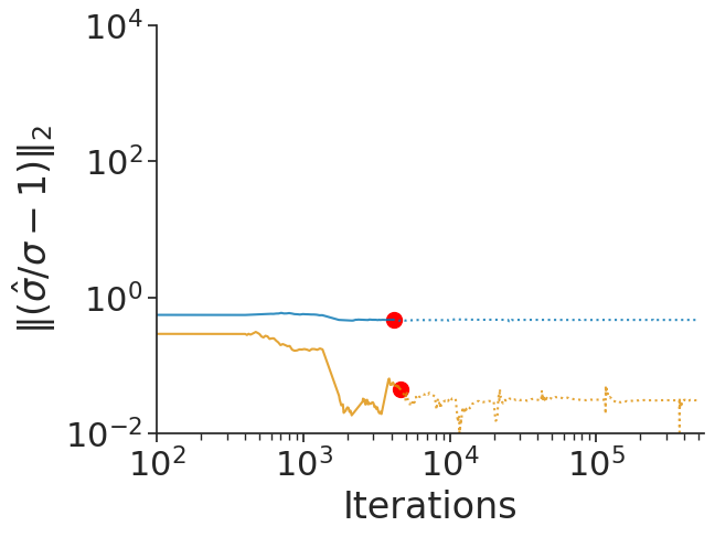
(d) dogs_log

(e) dogs

(f) diamonds

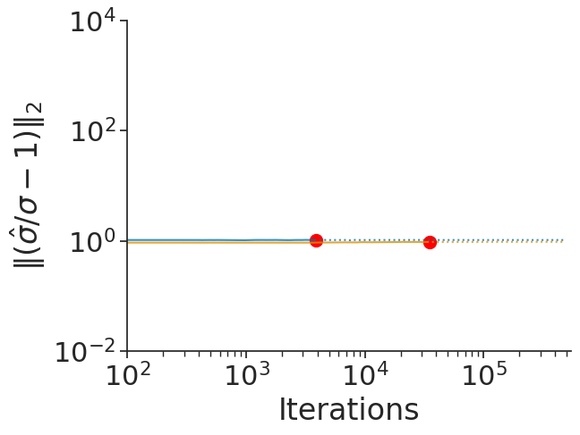
(g) 8schools_c

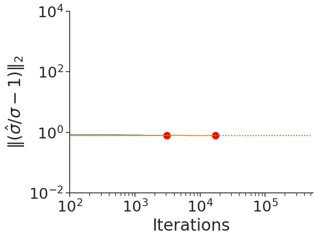
(h) 8schools_nc

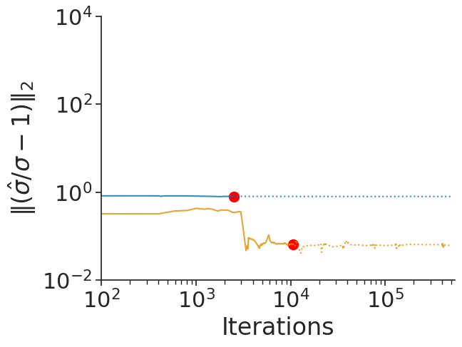
(i) hmm_example

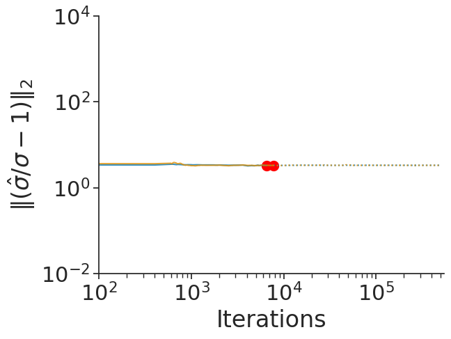
(j) low_dim_gauss

(k) nes2000

(l) sblrc

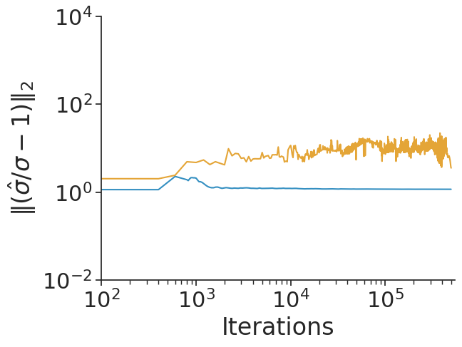
(m) earnings

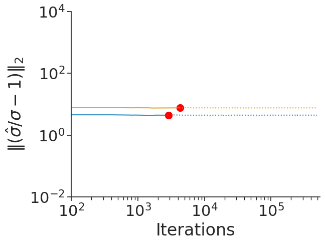
(n) garch

(o) gp_pois_regr

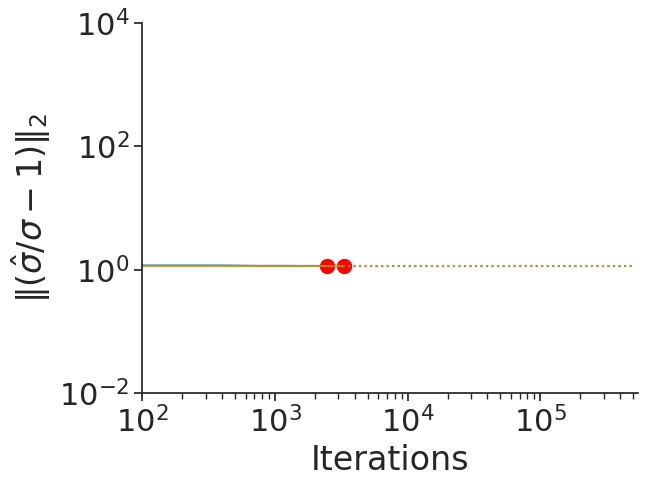
(p) gp_regr

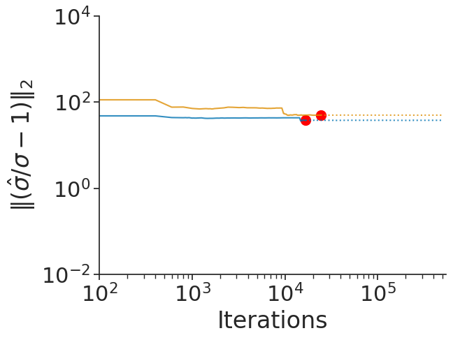
(q) hudson_lynx

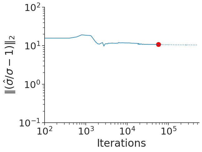
(r) mcycle_gp

Figure C.11: Accuracy of mean-field (blue) and full-rank (orange) Gaussian family approximations for selected posteriordb data/models, where accuracy is measured in terms of relative standard deviation error. The red dots indicate where the termination rule triggers

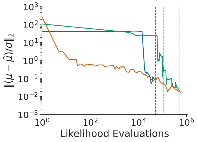
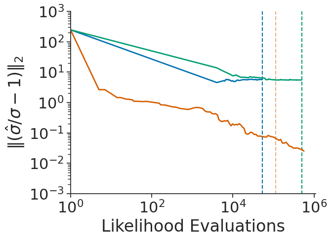
(a) arK

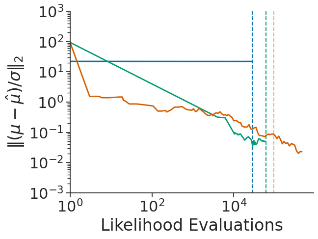
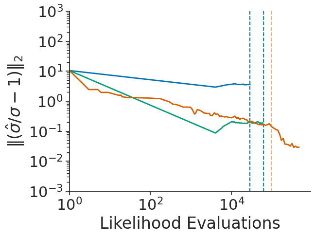
(b) bball_0

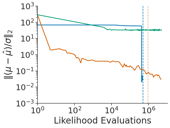
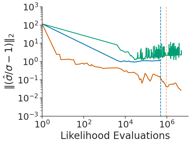
(c) bball_1

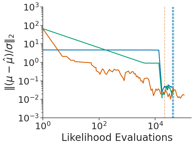
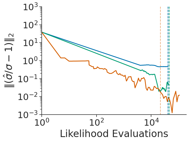
(d) dogs_logs

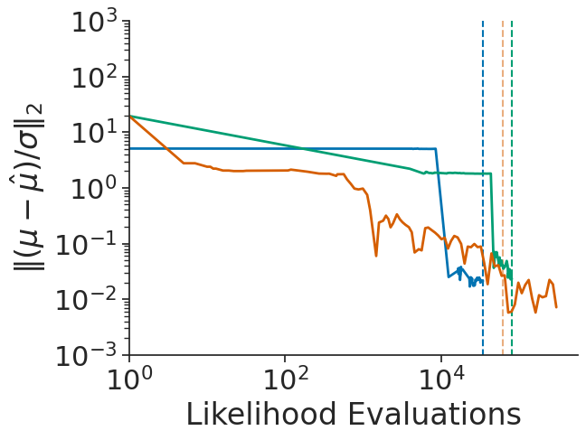
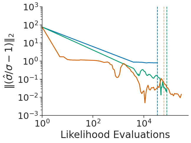
(e) dogs

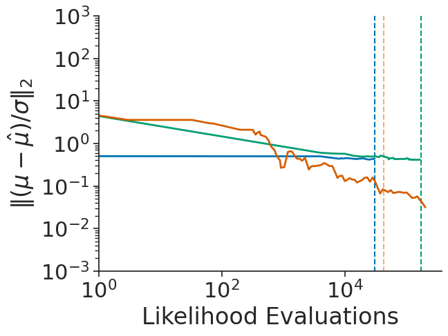
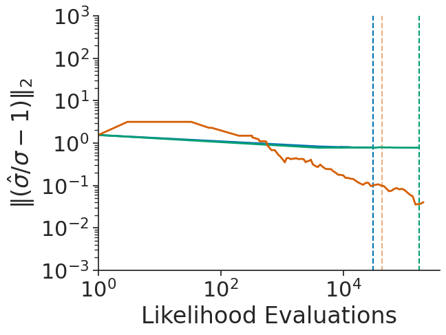
(f) 8schools_nc

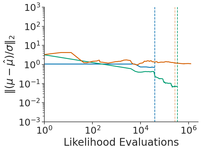
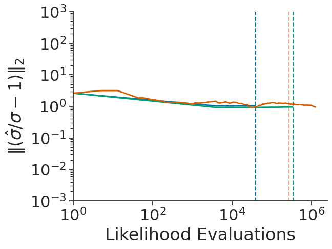
(g) 8schools_c

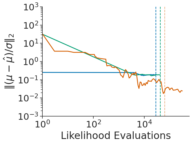
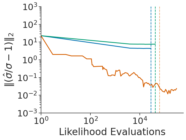
(h) garch

Figure C.12: Results of RAABBVI with mean-field Gaussian (blue) and full-rank Gaussian (green) family comparison to dynamic HMC (orange) in terms of relative mean error (top) and relative standard error (bottom). Blue and green vertical lines show the termination rule triggering points in RAABBVI and orange vertical line shows the end of warm-up period in dynamic HMC.

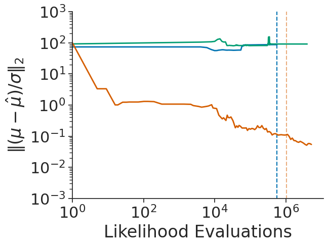
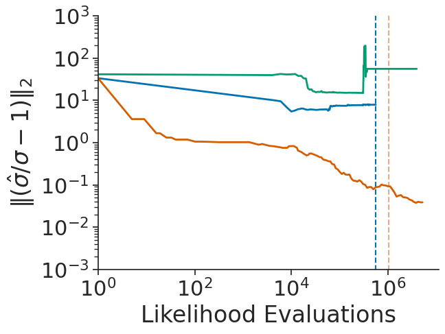
(a) gp_pois_regr

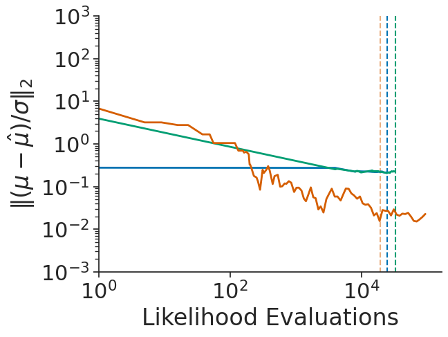
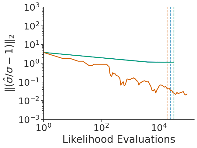
(b) gp_regr

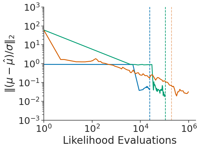
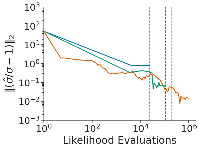
(c) hmm_example

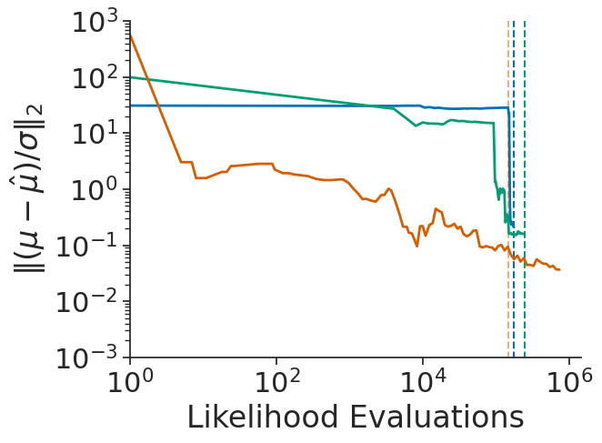
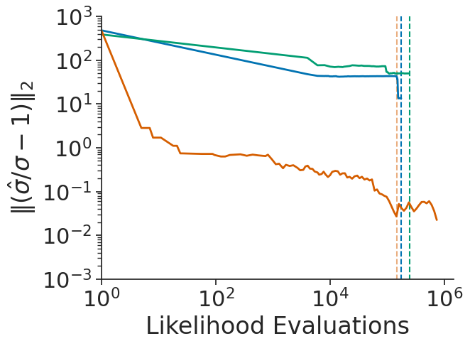
(d) hudson_lynx

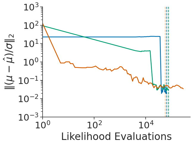
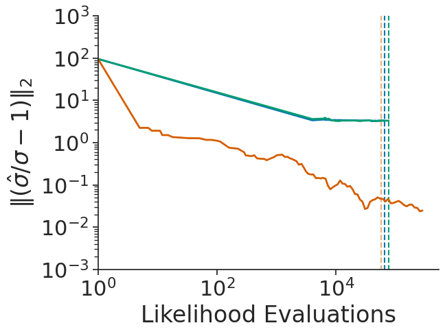
(e) low_dim_gauss

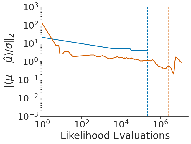
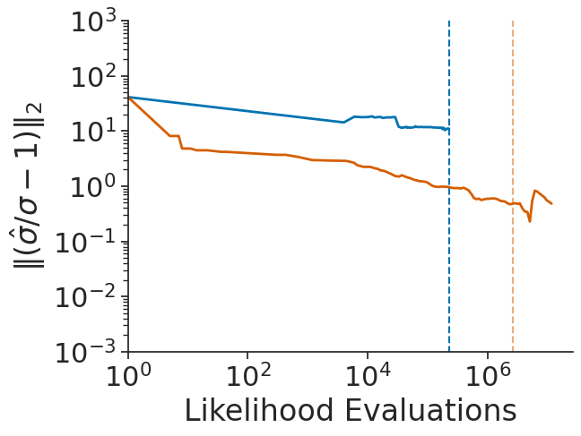
(f) mcycle_gp

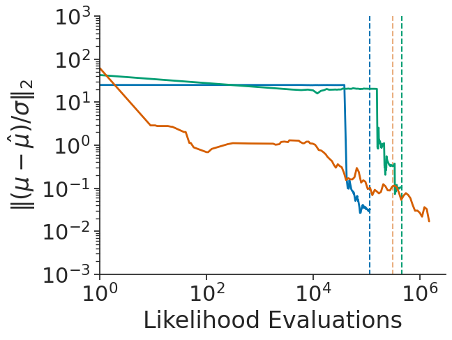
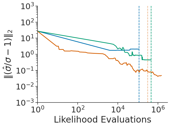
(g) nes2000

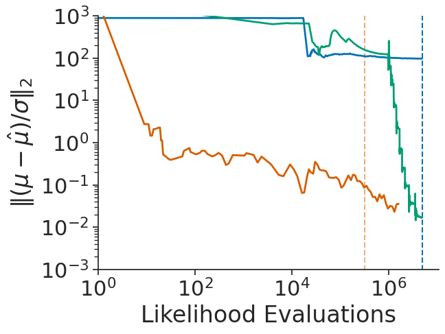
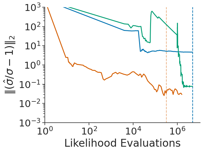
(h) sblrc

Figure C.13: Results of RAABBVI with mean-field Gaussian (blue) and full-rank Gaussian (green) family comparison to dynamic HMC (orange) in terms of relative mean error (top) and relative standard error (bottom). Blue and green vertical lines show the termination rule triggering points in RAABBVI and orange vertical line shows the end of warm-up period in dynamic HMC.

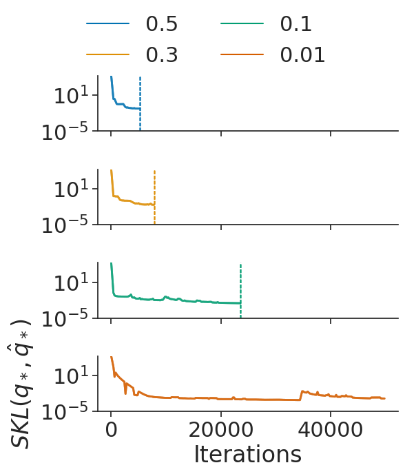
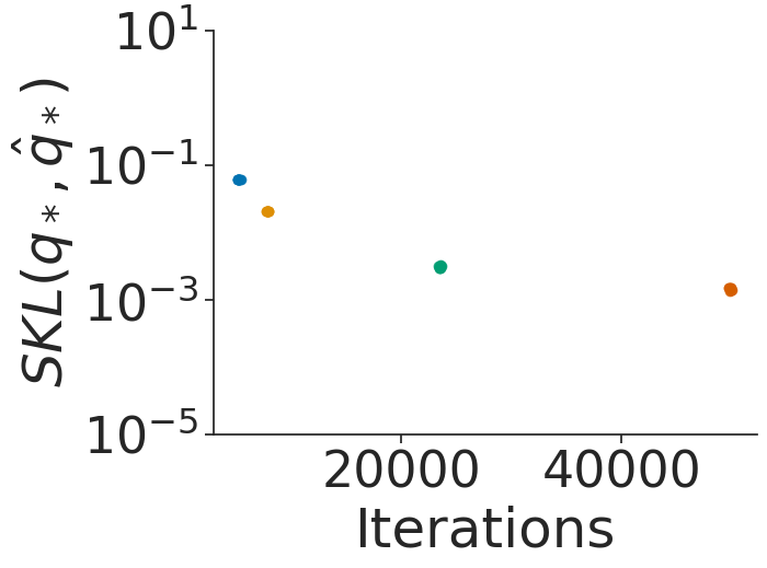
(a) uncorrelated $d=100$

(b) uncorrelated $d=500$

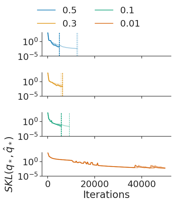
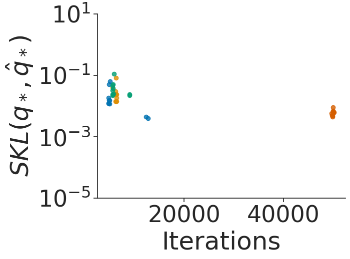
(c) uniform correlated $d=100$

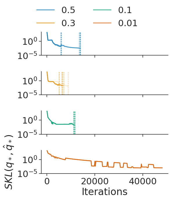
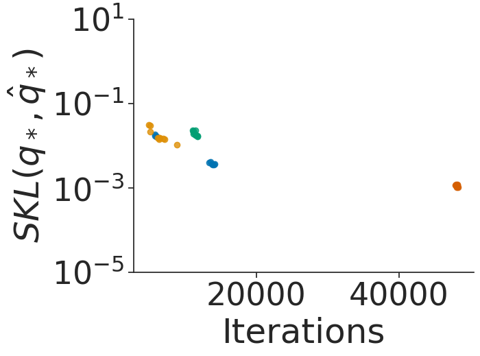
(d) banded correlated $d=100$

Figure C.14: Robustness to initial learning rate $\gamma_{0}$ using Gaussian targets. (top) Iterations versus symmetrized KL divergence between iterate average and optimal variational approximation. The distinct lines represent repeated experiments and the vertical lines indicate the termination rule trigger points. (bottom) Iterations versus symmetrized KL divergence between iterate average and optimal variational approximation at the termination rule trigger point.

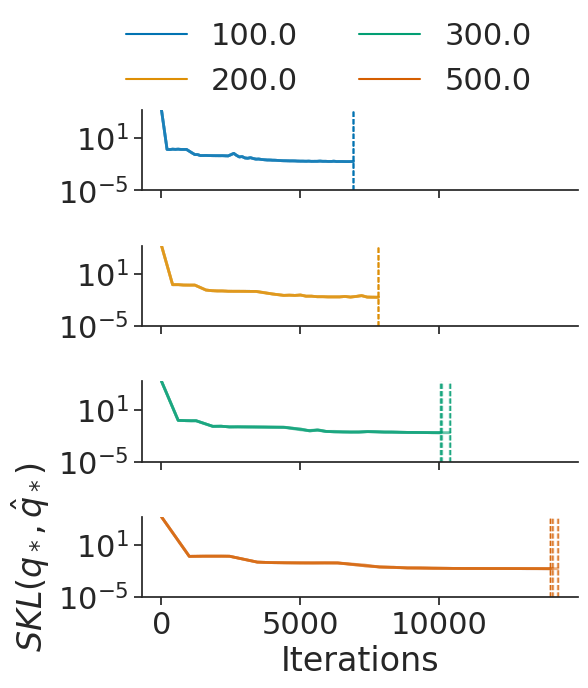
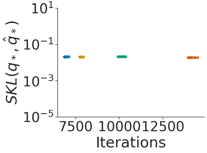
(a) uncorrelated $d=100$

(b) uncorrelated $d=500$

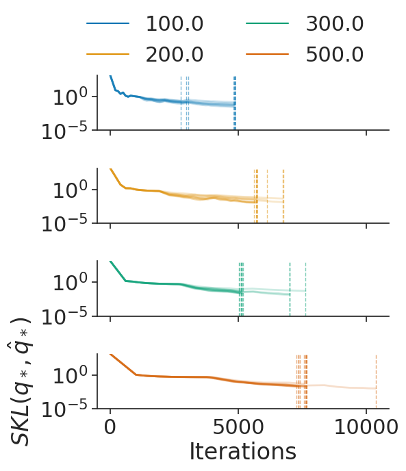
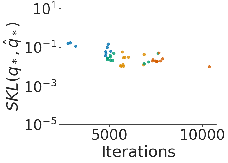
(c) uniform correlated $d=100$

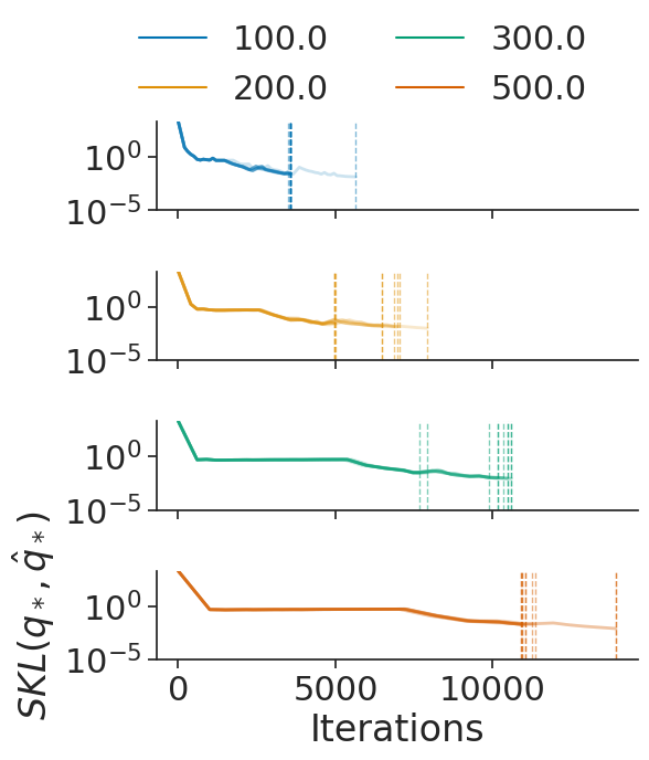
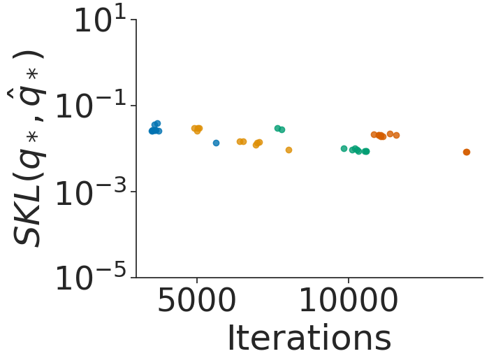
(d) banded correlated $d=100$

Figure C.15: Robustness to minimum window size $W_{min}$,, using Gaussian targets. (top) Iterations versus symmetrized KL divergence between iterate average and optimal variational approximation. The distinct lines represent repeated experiments and the vertical lines indicate the termination rule trigger points. (bottom) Iterations versus symmetrized KL divergence between iterate average and optimal variational approximation at the termination rule trigger point.

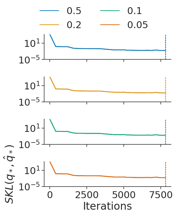
(a) uncorrelated $d=100$

(b) uncorrelated $d=500$

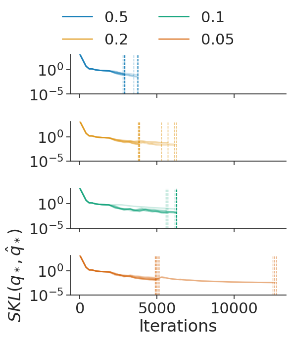
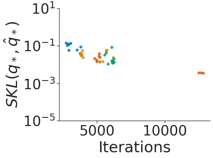
(c) uniform correlated $d=100$

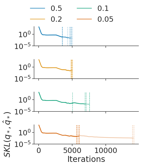
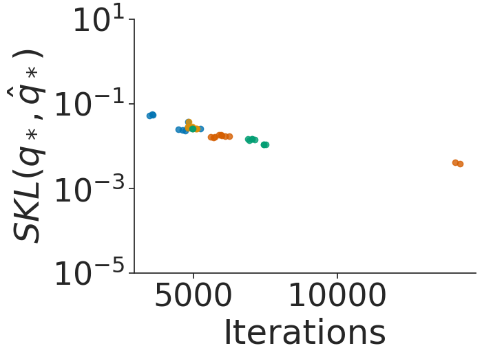
(d) banded correlated $d=100$

Figure C.16: Robustness to initial iterate average relative error threshold $\varepsilon$ using Gaussian targets. (top) Iterations versus symmetrized KL divergence between iterate average and optimal variational approximation. The distinct lines represent repeated experiments and the vertical lines indicate the termination rule trigger points. (bottom) Iterations versus symmetrized KL divergence between iterate average and optimal variational approximation at the termination rule trigger point.

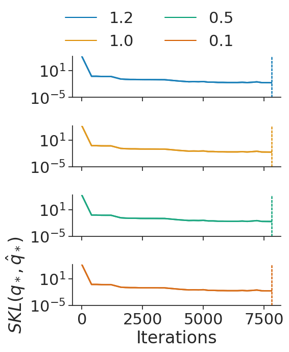
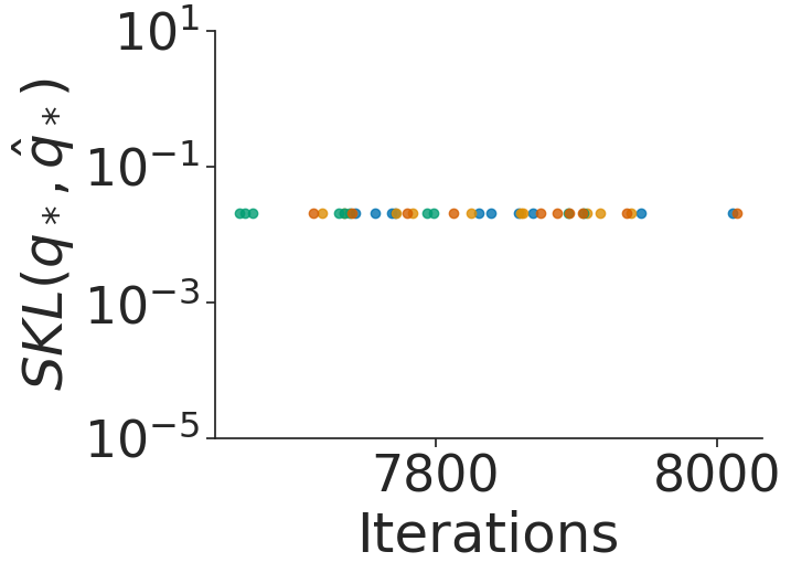
(a) uncorrelated $d=100$

(b) uncorrelated $d=500$

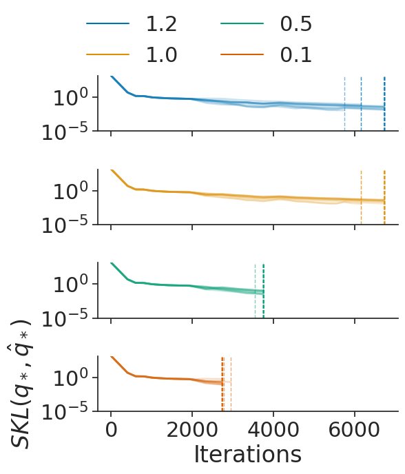
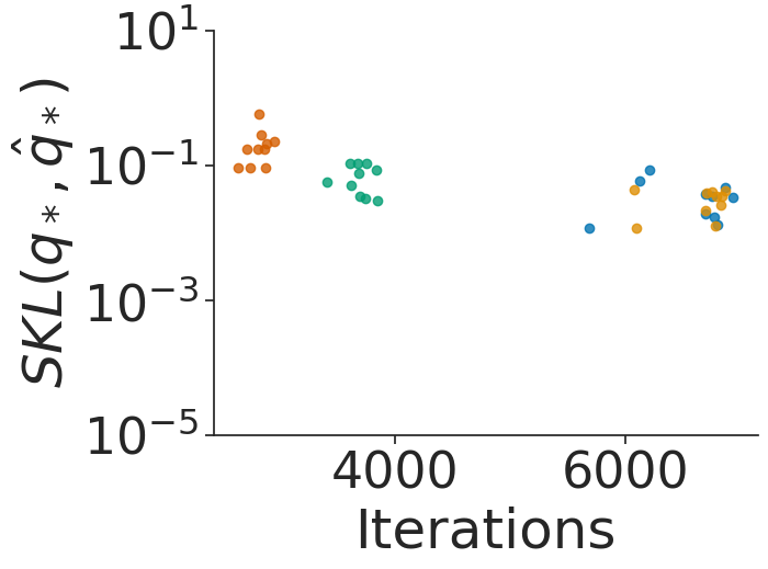
(c) uniform correlated $d=100$

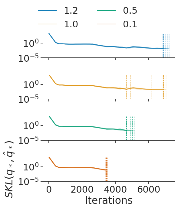
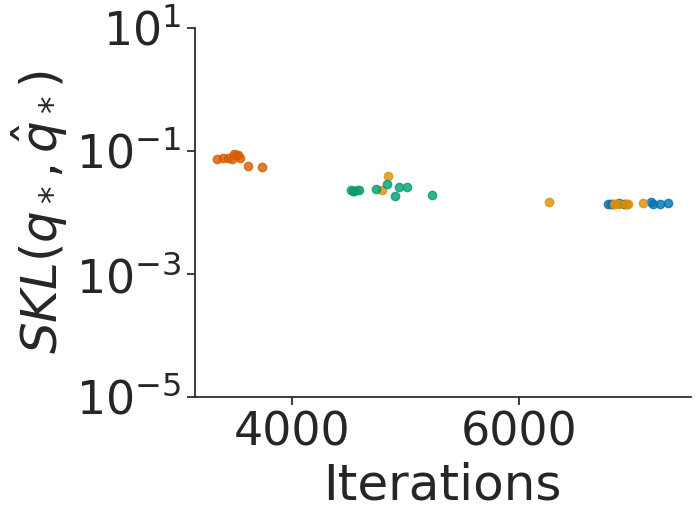
(d) banded correlated $d=100$

Figure C.17: Robustness to inefficiency threshold $\tau$ using Gaussian targets. (top) Iterations versus symmetrized KL divergence between iterate average and optimal variational approximation. The distinct lines represent repeated experiments and the vertical lines indicate the termination rule trigger points. (bottom) Iterations versus symmetrized KL divergence between iterate average and optimal variational approximation at the termination rule trigger point.

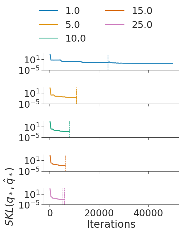
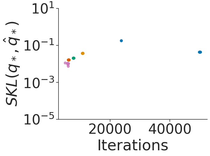
(a) uncorrelated $d=100$

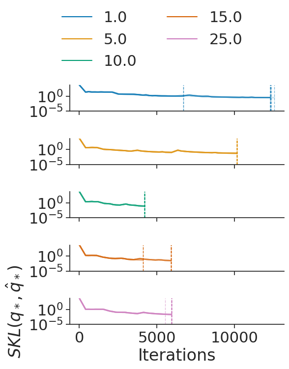
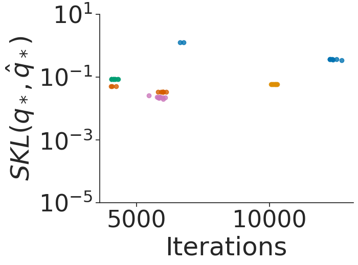
(b) uncorrelated $d=500$

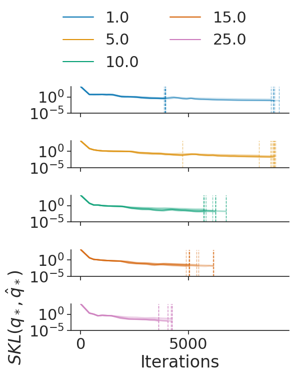
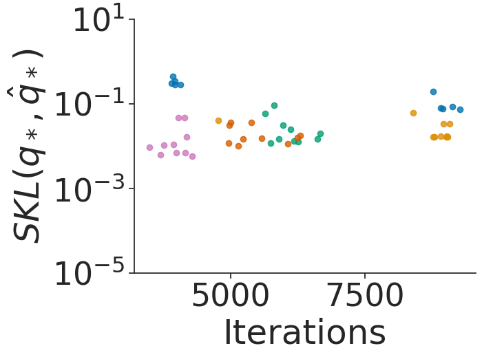
(c) uniform correlated $d=100$

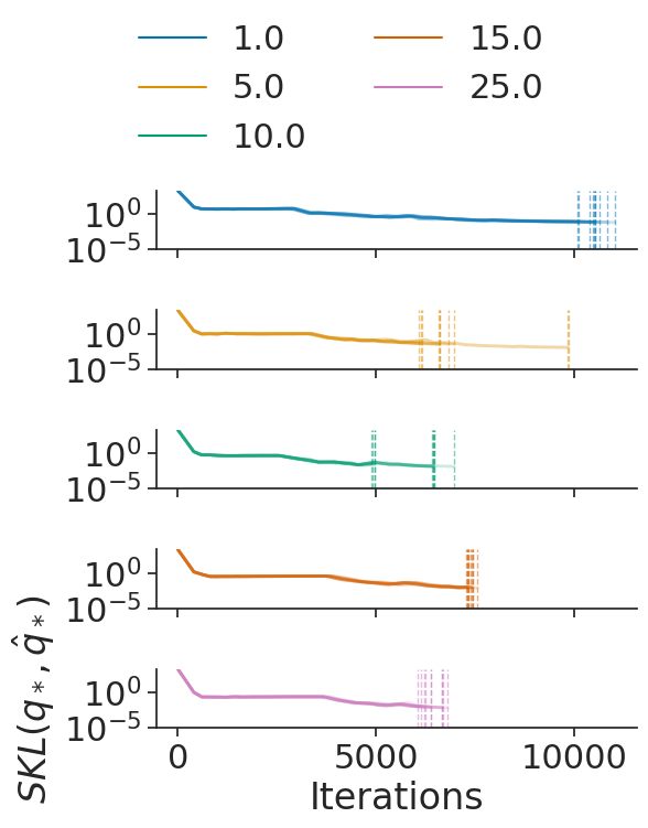
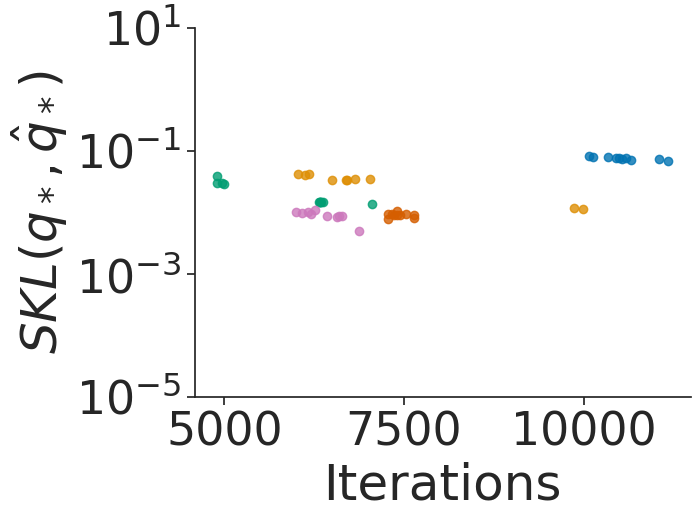
(d) banded correlated $d=100$

Figure C.18: Robustness to Monte Carlo samples $M$ using Gaussian targets. (top) Iterations versus symmetrized KL divergence between iterate average and optimal variational approximation. The distinct lines represent repeated experiments and the vertical lines indicate the termination rule trigger points. (bottom) Iterations versus symmetrized KL divergence between iterate average and optimal variational approximation at the termination rule trigger point.

References

- Agrawal, Sheldon and Domke [2020] {binproceedings}[author] \bauthor\bsnmAgrawal, \bfnmAbhinav\binitsA., \bauthor\bsnmSheldon, \bfnmDaniel\binitsD. and \bauthor\bsnmDomke, \bfnmJustin\binitsJ. (\byear2020). \btitleAdvances in Black-Box VI: Normalizing Flows, Importance Weighting, and Optimization. In \bbooktitleAdvances in Neural Information Processing Systems. \endbibitem
- Bach and Moulines [2013] {binproceedings}[author] \bauthor\bsnmBach, \bfnmF\binitsF. and \bauthor\bsnmMoulines, \bfnmE\binitsE. (\byear2013). \btitleNon-strongly-convex smooth stochastic approximation with convergence rate . In \bbooktitleAdvances in Neural Information Processing Systems \bpages1–9. \endbibitem
- Bishop [2006] {bbook}[author] \bauthor\bsnmBishop, \bfnmC. M.\binitsC. M. (\byear2006). \btitlePattern Recognition and Machine Learning. \bpublisherSpringer. \endbibitem
- Blei, Kucukelbir and McAuliffe [2017] {barticle}[author] \bauthor\bsnmBlei, \bfnmD. M.\binitsD. M., \bauthor\bsnmKucukelbir, \bfnmAlp\binitsA. and \bauthor\bsnmMcAuliffe, \bfnmJon D\binitsJ. D. (\byear2017). \btitleVariational Inference: A Review for Statisticians. \bjournalJournal of the American Statistical Association \bvolume112 \bpages859–877. \endbibitem
- Bolley and Villani [2005] {barticle}[author] \bauthor\bsnmBolley, \bfnmFrançois\binitsF. and \bauthor\bsnmVillani, \bfnmC\binitsC. (\byear2005). \btitleWeighted Csiszár-Kullback-Pinsker inequalities and applications to transportation inequalities. \bjournalAnnales de la faculte des sciences de Toulouse \bvolume13 \bpages331–352. \endbibitem
- Bubeck, Eldan and Lehec [2015] {binproceedings}[author] \bauthor\bsnmBubeck, \bfnmS\binitsS., \bauthor\bsnmEldan, \bfnmR\binitsR. and \bauthor\bsnmLehec, \bfnmJ\binitsJ. (\byear2015). \btitleFinite-Time Analysis of Projected Langevin Monte Carlo. In \bbooktitleAdvances in Neural Information Processing Systems. \endbibitem
- Bui, Yan and Turner [2017] {barticle}[author] \bauthor\bsnmBui, \bfnmThang D\binitsT. D., \bauthor\bsnmYan, \bfnmJosiah\binitsJ. and \bauthor\bsnmTurner, \bfnmRichard E\binitsR. E. (\byear2017). \btitleA Unifying Framework for Gaussian Process Pseudo-Point Approximations using Power Expectation Propagation. \bjournalJournal of Machine Learning Research \bvolume18 \bpages1–72. \endbibitem
- Burda, Grosse and Salakhutdinov [2016] {binproceedings}[author] \bauthor\bsnmBurda, \bfnmY\binitsY., \bauthor\bsnmGrosse, \bfnmRoger B\binitsR. B. and \bauthor\bsnmSalakhutdinov, \bfnmR\binitsR. (\byear2016). \btitleImportance Weighted Autoencoders. In \bbooktitleInternational Conference on Learning Representations. \endbibitem
- Chee and Li [2020] {barticle}[author] \bauthor\bsnmChee, \bfnmJerry\binitsJ. and \bauthor\bsnmLi, \bfnmPing\binitsP. (\byear2020). \btitleUnderstanding and Detecting Convergence for Stochastic Gradient Descent with Momentum. \bjournalarXiv.org \bvolumearXiv:2008.12224 [cs.LG]. \endbibitem
- Chee and Toulis [2018] {binproceedings}[author] \bauthor\bsnmChee, \bfnmJerry\binitsJ. and \bauthor\bsnmToulis, \bfnmPanos\binitsP. (\byear2018). \btitleConvergence diagnostics for stochastic gradient descent with constant learning rate. In \bbooktitleInternational Conference on Artificial Intelligence and Statistics. \endbibitem
- Chen et al. [2019] {barticle}[author] \bauthor\bsnmChen, \bfnmHuiming\binitsH., \bauthor\bsnmWu, \bfnmHo-Chun\binitsH.-C., \bauthor\bsnmChan, \bfnmShing-Chow\binitsS.-C. and \bauthor\bsnmLam, \bfnmWong-Hing\binitsW.-H. (\byear2019). \btitleA stochastic quasi-Newton method for large-scale nonconvex optimization with applications. \bjournalIEEE transactions on neural networks and learning systems \bvolume31 \bpages4776–4790. \endbibitem
- Cornebise, Moulines and Olsson [2008] {barticle}[author] \bauthor\bsnmCornebise, \bfnmJulien\binitsJ., \bauthor\bsnmMoulines, \bfnmE\binitsE. and \bauthor\bsnmOlsson, \bfnmJimmy\binitsJ. (\byear2008). \btitleAdaptive methods for sequential importance sampling with application to state space models. \bjournalStatistics and Computing \bvolume18 \bpages461–480. \endbibitem
- Dhaka et al. [2020] {binproceedings}[author] \bauthor\bsnmDhaka, \bfnmAkash Kumar\binitsA. K., \bauthor\bsnmCatalina, \bfnmAlejandro\binitsA., \bauthor\bsnmAndersen, \bfnmMichael Riis\binitsM. R., \bauthor\bsnmMagnusson, \bfnmMåns\binitsM., \bauthor\bsnmHuggins, \bfnmJonathan H\binitsJ. H. and \bauthor\bsnmVehtari, \bfnmAki\binitsA. (\byear2020). \btitleRobust, Accurate Stochastic Optimization for Variational Inference. In \bbooktitleAdvances in Neural Information Processing Systems. \endbibitem
- Dhaka et al. [2021] {barticle}[author] \bauthor\bsnmDhaka, \bfnmAkash Kumar\binitsA. K., \bauthor\bsnmCatalina, \bfnmAlejandro\binitsA., \bauthor\bsnmWelandawe, \bfnmManushi\binitsM., \bauthor\bsnmAndersen, \bfnmMichael R\binitsM. R., \bauthor\bsnmHuggins, \bfnmJonathan\binitsJ. and \bauthor\bsnmVehtari, \bfnmAki\binitsA. (\byear2021). \btitleChallenges and Opportunities in High Dimensional Variational Inference. \bjournalAdvances in Neural Information Processing Systems \bvolume34. \endbibitem
- Dieng et al. [2017] {binproceedings}[author] \bauthor\bsnmDieng, \bfnmAdji B\binitsA. B., \bauthor\bsnmTran, \bfnmDustin\binitsD., \bauthor\bsnmRanganath, \bfnmRajesh\binitsR., \bauthor\bsnmPaisley, \bfnmJ.\binitsJ. and \bauthor\bsnmBlei, \bfnmD. M.\binitsD. M. (\byear2017). \btitleVariational Inference via Upper Bound Minimization. In \bbooktitleAdvances in Neural Information Processing Systems. \endbibitem
- Dieuleveut, Durmus and Bach [2020] {barticle}[author] \bauthor\bsnmDieuleveut, \bfnmAymeric\binitsA., \bauthor\bsnmDurmus, \bfnmAlain\binitsA. and \bauthor\bsnmBach, \bfnmF\binitsF. (\byear2020). \btitleBridging the Gap between Constant Step Size Stochastic Gradient Descent and Markov Chains. \bjournalThe Annals of Statistics \bvolume48 \bpages1348–1382. \endbibitem
- Duchi, Hazan and Singer [2011] {barticle}[author] \bauthor\bsnmDuchi, \bfnmJohn\binitsJ., \bauthor\bsnmHazan, \bfnmElad\binitsE. and \bauthor\bsnmSinger, \bfnmYoram\binitsY. (\byear2011). \btitleAdaptive Subgradient Methods for Online Learning and Stochastic Optimization. \bjournalJournal of Machine Learning Research \bvolume12 \bpages2121–2159. \endbibitem
- Durmus, Majewski and Miasojedow [2019] {barticle}[author] \bauthor\bsnmDurmus, \bfnmAlain\binitsA., \bauthor\bsnmMajewski, \bfnmSzymon\binitsS. and \bauthor\bsnmMiasojedow, \bfnmBlazej\binitsB. (\byear2019). \btitleAnalysis of Langevin Monte Carlo via convex optimization. \bjournalJournal of Machine Learning Research \bvolume20 \bpages1–46. \endbibitem
- Durmus and Moulines [2019] {barticle}[author] \bauthor\bsnmDurmus, \bfnmAlain\binitsA. and \bauthor\bsnmMoulines, \bfnmE\binitsE. (\byear2019). \btitleHigh-dimensional Bayesian inference via the unadjusted Langevin algorithm. \bjournalBernoulli \bvolume25 \bpages2854–2882. \endbibitem
- Eberle and Majka [2019] {barticle}[author] \bauthor\bsnmEberle, \bfnmAndreas\binitsA. and \bauthor\bsnmMajka, \bfnmMateusz B\binitsM. B. (\byear2019). \btitleQuantitative contraction rates for Markov chains on general state spaces. \bjournalElectronic Journal of Probability \bvolume24 \bpages1–36. \endbibitem
- Gal and Ghahramani [2016] {binproceedings}[author] \bauthor\bsnmGal, \bfnmYarin\binitsY. and \bauthor\bsnmGhahramani, \bfnmZ.\binitsZ. (\byear2016). \btitleDropout as a Bayesian Approximation - Representing Model Uncertainty in Deep Learning. In \bbooktitleInternational Conference on Machine Learning. \endbibitem
- Gelman and Rubin [1992] {barticle}[author] \bauthor\bsnmGelman, \bfnmAndrew\binitsA. and \bauthor\bsnmRubin, \bfnmDonald B\binitsD. B. (\byear1992). \btitleInference from iterative simulation using multiple sequences. \bjournalStatistical Science \bvolume7 \bpages457–511. \endbibitem
- Gelman et al. [2013] {bbook}[author] \bauthor\bsnmGelman, \bfnmAndrew\binitsA., \bauthor\bsnmCarlin, \bfnmJohn\binitsJ., \bauthor\bsnmStern, \bfnmHal\binitsH., \bauthor\bsnmDunson, \bfnmDavid B\binitsD. B., \bauthor\bsnmVehtari, \bfnmAki\binitsA. and \bauthor\bsnmRubin, \bfnmDonald B\binitsD. B. (\byear2013). \btitleBayesian Data Analysis, \beditionThird ed. \bpublisherChapman and Hall/CRC. \endbibitem
- Geyer [1992] {barticle}[author] \bauthor\bsnmGeyer, \bfnmC J\binitsC. J. (\byear1992). \btitlePractical Markov Chain Monte Carlo. \bjournalStatistical Science \bvolume7 \bpages473–483. \endbibitem
- Gitman et al. [2019] {binproceedings}[author] \bauthor\bsnmGitman, \bfnmIgor\binitsI., \bauthor\bsnmLang, \bfnmHunter\binitsH., \bauthor\bsnmZhang, \bfnmPengchuan\binitsP. and \bauthor\bsnmXiao, \bfnmLin\binitsL. (\byear2019). \btitleUnderstanding the Role of Momentum in Stochastic Gradient Methods. In \bbooktitleAdvances in Neural Information Processing Systems \bpages9633–9643. \endbibitem
- Hernández-Lobato et al. [2016] {binproceedings}[author] \bauthor\bsnmHernández-Lobato, \bfnmJosé Miguel\binitsJ. M., \bauthor\bsnmLi, \bfnmYingzhen\binitsY., \bauthor\bsnmRowland, \bfnmMark\binitsM., \bauthor\bsnmBui, \bfnmThang D\binitsT. D., \bauthor\bsnmHernández-Lobato, \bfnmDaniel\binitsD. and \bauthor\bsnmTurner, \bfnmRichard E\binitsR. E. (\byear2016). \btitleBlack-Box Alpha Divergence Minimization. In \bbooktitleInternational Conference on Machine Learning. \endbibitem
- Hinton and Tieleman [2012] {binproceedings}[author] \bauthor\bsnmHinton, \bfnmG. E.\binitsG. E. and \bauthor\bsnmTieleman, \bfnmTijmen\binitsT. (\byear2012). \btitleLecture 6.5 – Rmsprop: Divide the gradient by a running average of its recent magnitude. In \bbooktitleCoursera: Neural networks for machine learning. \endbibitem
- Huggins et al. [2020] {binproceedings}[author] \bauthor\bsnmHuggins, \bfnmJonathan H\binitsJ. H., \bauthor\bsnmKasprzak, \bfnmMikolaj\binitsM., \bauthor\bsnmCampbell, \bfnmTrevor\binitsT. and \bauthor\bsnmBroderick, \bfnmT.\binitsT. (\byear2020). \btitleValidated Variational Inference via Practical Posterior Error Bounds. In \bbooktitleInternational Conference on Artificial Intelligence and Statistics. \endbibitem
- Johnson et al. [2016] {binproceedings}[author] \bauthor\bsnmJohnson, \bfnmMatthew J\binitsM. J., \bauthor\bsnmDuvenaud, \bfnmD\binitsD., \bauthor\bsnmWiltschko, \bfnmAlexander B\binitsA. B., \bauthor\bsnmDatta, \bfnmSandeep R\binitsS. R. and \bauthor\bsnmAdams, \bfnmR P\binitsR. P. (\byear2016). \btitleComposing graphical models with neural networks for structured representations and fast inference. In \bbooktitleAdvances in Neural Information Processing Systems. \endbibitem
- Joulin and Ollivier [2010] {barticle}[author] \bauthor\bsnmJoulin, \bfnmAldéric\binitsA. and \bauthor\bsnmOllivier, \bfnmYann\binitsY. (\byear2010). \btitleCurvature, concentration and error estimates for Markov chain Monte Carlo. \bjournalThe Annals of Probability \bvolume38 \bpages2418–2442. \endbibitem
- Khan and Lin [2017] {binproceedings}[author] \bauthor\bsnmKhan, \bfnmMohammad Emtiyaz\binitsM. E. and \bauthor\bsnmLin, \bfnmWu\binitsW. (\byear2017). \btitleConjugate-Computation Variational Inference : Converting Variational Inference in Non-Conjugate Models to Inferences in Conjugate Models. In \bbooktitleInternational Conference on Artificial Intelligence and Statistics. \endbibitem
- Kingma and Ba [2015] {binproceedings}[author] \bauthor\bsnmKingma, \bfnmDiederik P\binitsD. P. and \bauthor\bsnmBa, \bfnmJimmy\binitsJ. (\byear2015). \btitleAdam: A Method for Stochastic Optimization. In \bbooktitleInternational Conference on Learning Representations. \endbibitem
- Kingma and Welling [2014] {binproceedings}[author] \bauthor\bsnmKingma, \bfnmDiederik P\binitsD. P. and \bauthor\bsnmWelling, \bfnmMax\binitsM. (\byear2014). \btitleAuto-Encoding Variational Bayes. In \bbooktitleInternational Conference on Learning Representations. \endbibitem
- Kucukelbir et al. [2015] {binproceedings}[author] \bauthor\bsnmKucukelbir, \bfnmAlp\binitsA., \bauthor\bsnmRanganath, \bfnmRajesh\binitsR., \bauthor\bsnmGelman, \bfnmAndrew\binitsA. and \bauthor\bsnmBlei, \bfnmD. M.\binitsD. M. (\byear2015). \btitleAutomatic Variational Inference in Stan. In \bbooktitleAdvances in Neural Information Processing Systems. \endbibitem
- Lang, Zhang and Xiao [2019] {barticle}[author] \bauthor\bsnmLang, \bfnmHunter\binitsH., \bauthor\bsnmZhang, \bfnmPengchuan\binitsP. and \bauthor\bsnmXiao, \bfnmLin\binitsL. (\byear2019). \btitleUsing Statistics to Automate Stochastic Optimization. \bjournalarXiv.org \bvolumearXiv:1909.09785 [stat.ML]. \endbibitem
- Li and Turner [2016] {binproceedings}[author] \bauthor\bsnmLi, \bfnmYingzhen\binitsY. and \bauthor\bsnmTurner, \bfnmRichard E\binitsR. E. (\byear2016). \btitleRényi Divergence Variational Inference. In \bbooktitleAdvances in Neural Information Processing Systems \bpages1073–1081. \endbibitem
- Liu and Owen [2021] {barticle}[author] \bauthor\bsnmLiu, \bfnmSifan\binitsS. and \bauthor\bsnmOwen, \bfnmArt B\binitsA. B. (\byear2021). \btitleQuasi-Monte Carlo Quasi-Newton in Variational Bayes. \bjournalJournal of Machine Learning Research \bvolume22 \bpages1–23. \endbibitem
- Maddox et al. [2019] {binproceedings}[author] \bauthor\bsnmMaddox, \bfnmWesley\binitsW., \bauthor\bsnmGaripov, \bfnmTimur\binitsT., \bauthor\bsnmIzmailov, \bfnmPavel\binitsP., \bauthor\bsnmVetrov, \bfnmDmitry\binitsD. and \bauthor\bsnmWilson, \bfnmAndrew Gordon\binitsA. G. (\byear2019). \btitleA Simple Baseline for Bayesian Uncertainty in Deep Learning. In \bbooktitleAdvances in Neural Information Processing Systems. \endbibitem
- Madras and Sezer [2010] {barticle}[author] \bauthor\bsnmMadras, \bfnmNeal\binitsN. and \bauthor\bsnmSezer, \bfnmDeniz\binitsD. (\byear2010). \btitleQuantitative bounds for Markov chain convergence: Wasserstein and total variation distances. \bjournalBernoulli \bvolume16 \bpages882–908. \endbibitem
- Mohamed et al. [2020] {barticle}[author] \bauthor\bsnmMohamed, \bfnmShakir\binitsS., \bauthor\bsnmRosca, \bfnmMihaela\binitsM., \bauthor\bsnmFigurnov, \bfnmMichael\binitsM. and \bauthor\bsnmMnih, \bfnmAndriy\binitsA. (\byear2020). \btitleMonte Carlo Gradient Estimation in Machine Learning. \bjournalJournal of Machine Learning Research \bvolume21 \bpages1–62. \endbibitem
- Mukkamala and Hein [2017] {binproceedings}[author] \bauthor\bsnmMukkamala, \bfnmMahesh Chandra\binitsM. C. and \bauthor\bsnmHein, \bfnmMatthias\binitsM. (\byear2017). \btitleVariants of RMSProp and Adagrad with Logarithmic Regret Bounds. In \bbooktitleInternational Conference on Machine Learning. \endbibitem
- Murphy [2012] {bbook}[author] \bauthor\bsnmMurphy, \bfnmK\binitsK. (\byear2012). \btitleMachine Learning: A Probabilistic Perspective. \bpublisherMIT Press, \baddressCambridge, MA. \endbibitem
- Nocedal and Wright [2006] {bbook}[author] \bauthor\bsnmNocedal, \bfnmJorge\binitsJ. and \bauthor\bsnmWright, \bfnmStephen\binitsS. (\byear2006). \btitleNumerical optimization. \bpublisherSpringer Science & Business Media. \endbibitem
- Papamakarios et al. [2019] {barticle}[author] \bauthor\bsnmPapamakarios, \bfnmGeorge\binitsG., \bauthor\bsnmNalisnick, \bfnmEric\binitsE., \bauthor\bsnmRezende, \bfnmDanilo Jimenez\binitsD. J., \bauthor\bsnmMohamed, \bfnmShakir\binitsS. and \bauthor\bsnmLakshminarayanan, \bfnmBalaji\binitsB. (\byear2019). \btitleNormalizing Flows for Probabilistic Modeling and Inference. \bjournalarXiv.org \bvolumearXiv:1912.02762 [stat.ML]. \endbibitem