The aim of this paper is to develop the combinatorics of constructions associated to what we call triangular partitions. As introduced in [9], these are the partitions whose cells are those lying below the line joining points and , for any given positive reals and . Classical notions such as Dyck paths and parking functions are naturally generalized by considering the set of partitions included in a given triangular partition. One of our striking results is that the restriction of the Young lattice to triangular partition has a planar Hasse diagram, with many nice properties. It follows that we may generalize the “first-return” recurrence, for the enumeration of classical Dyck paths, to the enumeration of all partitions contained in a fixed triangular one.
Introduction
The last 30 years have seen increasing and interesting interactions between the combinatorics of generalized Dyck paths and parking functions, Macdonald polynomials and operators, diagonal coinvariant spaces, Hilbert schemes of points, Khovanov-Rozansky homology of -torus links, Double affine Hecke algebra, Elliptic Hall algebra, and Superspaces of bosons and fermions. The aim of this paper is to further the combinatorial study of the most general extension of the notion of Dyck paths that is involved in this context.
For the purpose of describing our overall setup, it is handy to consider classical Dyck paths as partitions contained in the staircase partition . These are well known to be enumerated by the Catalan numbers. From this point of view, parking functions are simply standard tableaux of skew shape , for any such . Recall that they number in total. The generalization we consider here is obtained by changing the overall partition to other suitably chosen partitions . For instance, one may consider the more the general staircase , for some . In that case, it is well known that the number of partitions included in is given by the Fuss-Catalan number . The corresponding number of parking functions is given by the simple formula . In the historical sequence of generalizations, Rational Catalan Combinatorics (see [1]) comes next in line, with an overall partition consisting in the set of cells lying below the diagonal of a -rectangle, with and coprime. The terminology “rational” alludes to being a rational number. Removing the coprimality condition, one gets Rectangular Catalan Combinatorics (see [5]).
The final step in the hierarchy, introduced in [9], corresponds to choosing any overall “triangular partition”. These are the partitions whose cells are those lying below the line joining points and , for any given positive reals and . The resulting partition111These are defined in Section 1., are here denoted by . As mentioned previously, the rational case corresponds to choosing and , relatively prime integers, and it is well known that the number of partitions contained in is given by the formula ,
whilst the number of associated parking functions is .
These enumerations become a bit trickier when one drops the coprimality requirement222This is the “rectangular” case., taking the respective forms
where , , for ; and writing for being a part of . Recall here that , with being the number of -size parts of .
The extension to any triangular partitions, when and are any positive real numbers, is motivated by the results in [9]. The purpose of this paper is to explore different aspects of this most general framework.
We start with a discussion of properties and intrinsic characterization triangular partitions, including interesting aspects of the dominance and containment order. We then obtain general recurrence for the (weighted) enumeration of triangular Dyck paths and associated parking functions (see Propositions 5.1 and 7.1).
1. Triangular partitions
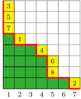
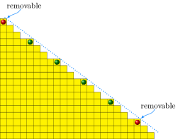
Figure 1.1. Triangular partition.
A partition is said to be triangular if there exists positive real numbers and such that
with running over integers that are less or equal to .
In other words, the cells of the triangular partition are those that lie below the line joining to , i.e.
We say that this line cuts off .
Clearly, the conjugate of a triangular partition is triangular.
Triangular partitions have been considered under the name “plane corner cuts” in [15], and enumerated in [10]. Denoting by the number of triangular partitions of size , small values of the sequence are:
Table 1.1 displays all triangular partitions of , with denoting the “empty” partition.
Table 1.1. All triangular partitions, for .
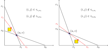
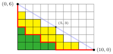
Observe that many different pairs may give rise to the same triangular partition . Indeed, as illustrated in Figure 1.3, we have whenever there are no positive integer coordinate points lying between the lines and .
In particular, for all and .
We say that the line touches the cell (from above) if it contains the north-east corner of the cell, i.e. .
If the line touches no cells, then for any close enough to . If the line touches a cell , then taking and , for a sufficiently small positive , one may “remove” the cell from the diagram of the partition. On the other hand, taking and we get a line cutting off the same partition while touching no cells. Summing up, for every triangular partition there is a pair such that the line cuts off , without touching any cell.
Let us say that is integral, if there exist and in such . As mentioned previously, these are the triangular partitions which give rise to the previous context of “rectangular” Catalan combinatorics; and adding the requirement that that of “rational” Catalan combinatorics. Clearly conjugation preserves integrality. For size , the non-integral triangular partitions are the following:
As grows, non-integral triangular partitions become preponderant. For instance, among all triangular partitions of size at most , more than of them are non-integral. Thus triangular partitions significantly extend the field of study.
A slope vector for a triangular partition is a positive coordinate vector which is orthogonal to one of the lines that cut off . If need be, we may normalize slope vectors so that their coordinates sum up to .
For any two lines cutting of the same triangular partition , say with respective slope vectors and , there exist a line with slope vector that also cuts of for any . By definition, a triangular partition affords (infinitely many) slope vectors. Hence, it follows that:
Lemma 1.1.
The closure of the set of all slope vectors of a triangular partition forms a convex cone , of the form
(1.1)
for some . Moreover, is uniquely characterized by its size and the pair .
We will further discuss this unicity below, but first we show how to explicitly calculate and . As we will see, this also gives a direct characterization of triangular partitions, without having to exhibit a cutting line.
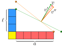
Figure 1.2. The two extreme slope vectors (here upscaled) of a hook shape .
For a cell of a partition , recall that the hook of is the partition of shape , with and standing for the arm and leg of of . Recall that (resp. ) is the number of cells of that sit to the right of (resp. above) in the same row (resp. column). The hook length of cell in , is defined to be . The “Frobenius notation” for such a hook is .
For any given cell of a partition , we consider the vectors and respectively orthogonal to the lines:
•
which joins the vertices and , and
•
which joins the vertices and .
An instance is illustrated in Figure 1.2.
It is easy to check that
(1.2)
When is a triangular partition, all of its slope vectors must be such that . Indeed, all the cells appearing in the hook of must lie below (up to parallel shift) any line that cuts off , with and giving extreme bounds. Otherwise, an extra cell would have to lie in , either at the end of the arm or the leg of .
Vice versa, if the condition is satisfied for every cell in , then is a slope vector of . Indeed, consider the lowest line perpendicular to and such that . It follows that the line touches a cell of of . Suppose that there is a cell that fits under the line , but such that . Without loss of generality, we can assume that lies to the west of . Let be the cell in the same column as and the same row as . Then which is a contradiction. Hence there is no such cell and We have thus shown the following:
Lemma 1.2.
A partition is triangular if and only if , with
(1.3)
Furthermore, if then is a slope vector of if and only if
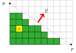
As illustrated in Figure 1.3, this gives an explicit description for the extreme rays of the cone which does not rely on an explicit knowledge of a line cutting off . Setting , we may consider the vector to be a “standard” slope vector for .
Figure 1.3. The cone of a triangular partition.
Two triangular partitions are said to be similar333Careful, this is not intended to be an equivalence relation. if they share a slope vector. For any triangular partition , it is easy to check that all partitions associated to -shadows of a cell :
are similar to . For any fixed , all the partitions with cell sets:
are clearly similar, since they share the slope vector . These partitions are nested as grows. Furthermore, if one chooses so that is irrational, cells are added one at a time as grows. We get the following
Corollary 1.1.
For a fixed size there are finitely many values
such that for every no triangular partition of size admits a slope vector . Furthermore, for every there is a unique triangular partition of size such that and .
Note
Part of the study of triangular partitions may be coined in terms of “sturmian” words. Indeed, these give explicit descriptions of discrete lines in the plane. Their factors, also known as “mechanical” word, describe segments of discrete lines. The upper bound (cells closest to a cutting line) of triangular partitions correspond to such segment. However, this approach does not emphasize the number of cells lying below the line. For more on sturmian and mechanical words, see [13, Chapter 2].
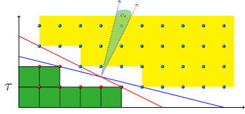
2. Moduli space of lines
Note that a line touches a cell if and only if
Therefore the positive -quadrant is can be decomposed into regions by (positive branches of) hyperbolas with equations as above, one for each cell. Thus may be considered as a moduli space of lines. In this moduli space, the hyperbola
associated to a cell , separates according to whether the cell fits below the line , is touched by the line , or does not fit under it. These possibilities respectively correspond to
Thus the cells occurring in a triangular partition specified by are in bijection with the hyperbolas separating from the origin. In other words, as one crosses the hyperbola , going towards the origin, the cell gets removed from the partition. For this reason it is natural to say that is the hyperbolic wall associated to .
Lemma 2.1.
There is a bijective natural map444Illustrated in Figure 2.1. , from the set of connected components of the complement:
to the set of triangular partitions.
(a)With regions labeled
(b)Larger portion
Figure 2.1. Triangular partition regions, in logarithmic scale.
Proof.
Consider the map that sends the -line in to the partition .
As observed above, this is a locally constant map from to the set of triangular partitions. Therefore, it is well defined on connected components. The surjectivity is immediate, since by definition a triangular partition is cut off by some line , and we have observed that may be chosen so that this line contains no points of .
To prove injectivity one needs to show that whenever two points of define the same triangular partition, then they must lie in the same connected component. We consider two cases.
First, when the lines associated to and do not intersect in the positive quadrant, then one may assume without loss of generality that and . Let us show that the segment , connecting these two points of , lies entirely within the same connected component of . Indeed, if the segment would cross one of the hyperbolic walls , then there would exist some such that the line passes through . The partition corresponding to would thus contain the cell , whereas the partition corresponding to would not; which is a contradiction.
If the lines associated to and intersect in the positive quadrant (as illustrated in Figure 2.2), say at some (non-integer) point , then both points and belong to the hyperbola . As one moves along this hyperbola, associated lines rotate around . Without loss of generality, one may assume that and . Consider the segment of the hyperbola lying between the points and . Suppose that for some point on this segment the line passes through an integer point . If , then it follows that the triangular partition corresponding to contains the cell , whereas the partition corresponding to does not. Similarly, if , then the triangular partition corresponding to contains the cell , whereas the partition corresponding to does not. Moreover, since the hyperbola can only intersect a vertical line at one point. Therefore, we get a contradiction in this case as well.
∎
Let be a triangular partition, and set
This is the closure of the connected component corresponding to by the above lemma. Observe that, for any in the interior , the line does not touch any cells. With this terminology, the bijective map of 2.1 sends .
We say that a cell of a triangular partition is removable
if it can be removed
so that the resulting partition is also triangular. Similarly, we say that a cell of the complement of is addable if it can be added to so that the resulting partition is also triangular. An argument similar to the proof of 2.1 proves the following:
Lemma 2.2.
Let be a removable cell of a triangular partition . Then there exists such that is the unique cell touched by the line .
Proof.
Consider such that the line cuts off , and such that the line cuts off . If these lines do not intersect in the positive quadrant, then , , and is the only integer point that lies between the lines. Then for some , with and , the line cuts off and touches the cell , while not touching any other cells.
Suppose the lines and intersect at some positive point . One can choose these lines so that they do not pass through integer points, ensuring that is not integral. Let us assume that (the case is obtained similarly). The triangle bounded by the lines and the vertical axis contains the unique integer point , while the triangle bounded by the lines and the horizontal axis does not contain integer points. Therefore, the line connecting and cuts off and touches the unique cell .
∎
The following Lemma can be observed directly, but it is especially natural from the point of view of the moduli space of lines :
Lemma 2.3.
Consider a line . Let be all the cells touched by , ordered so that . Then the set of triangular partitions such that is the union of the following:
(1)
(2)
(3)
(4)
Indeed, there are hyperbolas intersecting at , and these partitions correspond to the connected components of near . Note that only two of the cells in are removable: and . In cases and of the Lemma the only removable cell touched by the line is . Similarly, of the cells only and are addable for , and in the cases and the only addable cells touched by the line are and respectively.
3. Orders on triangular partitions
Two orders are of interest here, both obtained by restriction of classical orders on partitions to triangular partitions.
First, even though the dominance order is only a partial order on all partitions of a given size555Starting with size 6., its restriction to triangular partitions is a total order which we denoted by . See Figure 3.1 for an illustration of the difference between the two contexts.
Figure 3.1. The dominance order on all partitions of , and its restriction to triangular ones.
It is easy to show that
Lemma 3.1.
For two same size triangular partitions and , we have if and only if . Furthermore, covers in dominance order if and only if .
Proof.
According to 1.1, is not a slope vector of any triangular partition of size if and only if there exist triangular partitions and of size , such that . Let be the closest to the origin line with the slope vector such that . It follows then that touches more then one cell. Similar to 2.3, let be all the cells touched by , ordered so that . Let . One gets by the definition of the line . Partition is of size and can be cut off by a line with a slope vector for a small enough . Indeed, one should rotate the line counterclockwise around the north-east corner of the cell a little. Therefore, . By a similar consideration, one can obtain that . Finally, one observes that and the rest of the Lemma follows from 1.1.
∎
In simple terms, if one lists same size triangular partitions in clockwise order of their slope vectors, they will occur in decreasing dominance order. For size , this is illustrated in Figure 3.1.
More properties of the dominance order on triangular partitions (with a different terminology) may be found in [14].
Our second order of interest is the restriction of the containment order to triangular partitions. This gives rise to the Triangular Young poset, which we denoted by . We denote the cover relation in by .
Lemma 3.2.
Let and be triangular partitions and Then one has if and only if is obtained from by removing exactly one cell. In particular, is ranked by the number of cells in a partition.
Proof.
Clearly, if is obtained from by removing exactly one cell, then Suppose now that and Let and Similar to Lemma 2.1, let us connect the points and of the moduli space by a path as follows: if the corresponding lines do not intersect inside the positive quadrant, then take the straight line if they intersect, then take they rotation around the point of intersection. Observe that in both cases the partition can only increase as increases. Indeed, even for the rotation, if a cell gets removed, it is not going to be added back later, which contradicts Since it follows that all cells from have to be added simultaneously, at a certain value which means that the line touches all the cells of But then Lemma 2.3 guarantees that the cells, in fact, can be added one by one. Contradiction.
∎
Corollary 3.1.
Modulo the map from 2.1, the cover relation of corresponds to crossing an hyperbolic wall at a generic point.
In other words, the Hasse diagram of is planar: for every triangular partition one can draw the vertex corresponding to it at the center of the region and then connect vertices in the neighboring regions by crossing the shared pieces of the boundary at simple points. Note that the resulting drawing of the Hasse diagram satisfies an additional condition:
Lemma 3.3.
For any interval the vertices corresponding to and in the planar presentation of the Hasse diagram of obtained by restricting the above construction to both belong to the boundary of the unbounded region. In particular, the graph obtained from the Hasse diagram of by adding an extra edge connecting to is planar.
Proof.
Indeed, the regions corresponding to the partitions not in the interval are inside the unbounded region of the Hasse diagram of and unless both and share boundaries with regions corresponding to partitions outside of If then the corresponding vertex is also clearly on the boundary of the unbounded region.
∎
In the drawing of the Hasse diagram as above the triangular partitions with the same number of cells appear in the decreasing dominance order, from left to right.
There is a subtle difference between the planarity of the Hasse diagram as an abstract graph and its planarity as a Hasse diagram: in a Hasse diagram the edges are required to be drawn going upward from the smaller element to the bigger element, with respect to a chosen direction. See [16] for a detailed discussion of the planarity of Hasse diagrams and its connection to the condition in Lemma 3.3.
Lemma 3.4.
The poset is a lattice.
Proof.
Since is bounded from below, it suffices to show that the join operation is well defined. Clearly, for any two triangular partitions and there exist a common upper bound, i.e. a triangular partition such that and Therefore, we only need to prove that the minimal upper bound is unique.
Suppose that are two minimal upper bounds for and Consider a saturated chain connecting to and let be the maximal element on that chain such that Similarly, consider a saturated chain connecting to and let be the maximal element on that chain such that Consider also saturated chains connecting to and to Note that all four chains connecting and to and cannot intersect each other except at the ends. In particular, they correspond to non-intersecting paths on the Hasse diagram.
Let be a minimal upper bound for and let be a maximal lower bound for and and consider saturated chains connecting to and and and to Note that the corresponding paths on the Hasse diagram do not intersect between each other or with the previously constructed four paths (except at the ends). Finally, Lemma 3.3 guaranties that if we restrict the drawing of the Hasse diagram to the interval than the vertices corresponding to and are going to be on the boundary of the unbounded region, and, therefore, can be connected by an extra path not intersecting any edges of the Hasse diagram of the interval Thus we obtained a planar presentation of a graph: every vertex of is connected to every vertex of and all the connecting paths do not intersect each other except at the ends. Contradiction.
∎
(a)With labeled nodes
(b)Larger portion
Figure 3.2. Bottom of Triangular Young poset (red vertices non-integral).
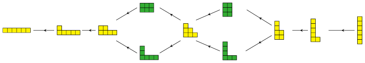
A lower portion of this Hasse diagram is illustrated in Figure 3.2. Its dual corresponds to Figure 2.1.
For obvious reasons, nodes and regions are unlabelled in the larger right-hand side images. The larger image of the poset displays all triangular partitions of . Its vertices are equal to (up to a logarithmic rescaling and rotation), with the standard666See definition after 1.2. slope vector of . The lattice is not a distributive, as illustrated by the fact that we have .
Let us prove a few more results about the triangular Young poset and the structure of the moduli space of lines
Lemma 3.5.
No triangular partition can have more than removable cells. Similarly, no triangular partition can have more than addable cells.
Proof.
Suppose that a triangular partition has three removable cells , , and , . It follows that the cell cannot fit under the line touching the cells and . Otherwise, in order to remove the cell one would either have to remove the cell or .
Without loss of generality, one may assume that , which implies . There is then a cell
since and
Consider the lines and respectively cutting off and . The cell fits under the line , but it does not fit under the line ; hence we have a contradiction. The statement about addable cells is proved analogously. ∎
One case of 3.5 is illustrated in Figure 3.3. Here the line cuts off and the line cuts off . Then the box fits under , but not under
Lemma 3.6.
Suppose that a triangular partition corresponds to an unbounded region. Then is either empty, a row partition, or a column partition.
Proof.
Indeed, if both cells and are in then both the leg and the arm of in are positive. 1.2 then implies that there exist such that if the line cuts off then . Also, if is an addable cell, then the hyperbolic wall is an upper boundary of the corresponding region. But then, the region has to lay inside the curved triangle bounded by the lines and , and the hyperbola
∎
Lemma 3.7.
Any bounded region is either a triangle or a quadrilateral. Each quadrilateral region has two lower boundaries and two upper boundaries, and they cannot alternate, i.e. the two lower boundaries intersect in a vertex of the region, and the two upper boundaries intersect in a vertex of the region.
Proof.
A bounded region cannot have just two boundaries, since two hyperbolic walls cannot intersect at more than one point (that would correspond to two distinct lines passing through the same two points). In view of 3.5, the only thing left to check is that a quadrilateral region cannot have sides alternating between lower and upper boundaries.
Let us follow the boundary of a region in the counterclockwise direction, and suppose that at a certain vertex we have a change in the type of the boundary (from lower to upper, or vice-versa). Let be the hyperbola that we followed approaching the vertex, and let be the hyperbola we followed after the vertex. Perforce, we have . Indeed, when moving counterclockwise along a lower boundary, is decreasing and is increasing, hence the corresponding line is rotating counterclockwise around . For the next boundary to be upper, one has to hit the north-east corner of an addable cell , which has to lie to the east of since the line is rotating counterclockwise. The case when the boundary changes from upper to lower is similarly dealt with. One concludes that the upper and lower boundaries cannot always alternate as one moves around the region.
∎
Lemma 3.8.
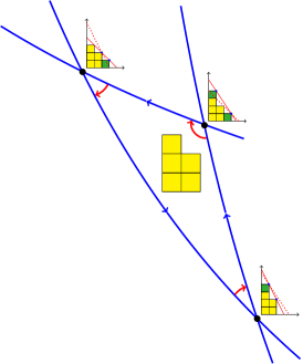
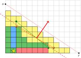
Let be a triangular partition corresponding to a quadrilateral region, which is to say that it has two removable and two addable cells. Then the line touching the two removable cells is parallel to the line touching the two addable cells777In Figure 2.1 this is reflected by the fact that lines connecting the top and the bottom corners of quadrilateral regions have slopes (in logarithmic scale)..
As illustrated in Figure 3.4, if one moves counterclockwise along the boundary of the ( sided) region corresponding to , then the corresponding line successively rotates
counterclockwise around the north-east corner of the removable cell (left),
clockwise around the north-east corner of the addable cell (center),
and clockwise around the addable cell (right).
In a transition from a lower boundary to an upper boundary (left) or vice versa (right), the center of rotation moves east. If the next piece of the boundary is of the same type (center), then the center of rotation moves west.
Proof.
Let be the line touching the two removable cells of , and let be the line touching the two addable cells of . 3.7 implies that . Let
be all the cells touched by , and let
be all the cells touched by . Since , according to 2.3 the cells are in , and and are the two removable cells of . Similarly, cells are not in , and and are the two addable cells of
Suppose that and are not parallel.Let be their intersection (here is not necessarily in the positive quadrant). Note that all the removable cells should fit below and none of the addable cells can fit below .It follows that is either to the east of the north-east corners of all addable and removable cells, or it is to the west of all of them. Without loss of generality one can assume that is to the east,i.e. and .It follows then that the line is steeper than
If there is a cell such that its north-east corner is strictly inside the triangle bounded by the horizontal axis and the lines and , then one gets a contradiction: this cell is strictly below , but cannot be inside since its north-east corner is above .
One needs to consider two cases. Suppose first that . Then there is a cell and its north-east corner is inside the required triangle. Indeed, one has:
and , so it is a cell, and its north-east corner is below and above , because we moved from the cell with the north-east corner on and above in the direction parallel to , which goes down steeper than
Suppose now that .Then there is a cell , and it is inside the required triangle. Indeed, one has:
and , so it is a cell, and its north-east corner is below and above because we moved from the cell with the north-east corner on and below in the direction parallel to , which goes down but less steep than
∎
Illustrated in Figure 3.5, are the cases when (left) and (right). Correspondingly, on the left and on the right . In both instances the cell creates a contradiction as it fits under but not under
Lemma 3.9.
Suppose that a triangular partition has two removable cells and just one addable cell (in other words it corresponds to a triangular region with two lower boundaries). Then the line touching the two removable cells does not contain any other positive integer points. Equivalently, no other hyperbolic wall passes through the vertex of the region where the two lower boundaries intersect.
Proof.
Suppose that two parallel lines and are such that
(1)
they both contain integer points,
(2)
there are no integer points (even not necessarily positive) between them,
(3)
contains finitely many positive integer points.
Then also contains finitely many positive integer points, and the numbers of positive integer points on and on differ not more than by one.
Now, let be the line touching the two removable cells of , and let be the line parallel to , above it, and satisfying the above conditions. Clearly, .The statement above then implies that contains at least one positive integer point. But if it contains more than one positive integer point, then by 2.3, the east-most and the west-most cells touched by are both addable. Contradiction. Therefore, contains exactly one positive integer point. But then cannot contain more than two.
∎
Lemma 3.10.
Suppose that a triangular partition has just one removable cell and two addable cells (in other words it corresponds to a triangular region with two upper boundaries). Then the line touching the two addable cells does not contain any other positive integer points. Equivalently, no other hyperbolic wall passes through the vertex of the region where the two upper boundaries intersect).
Figure 3.6. The diagonal of is the segment bounded by its removable cells.
The diagonal of triangular partition , is the set of cells that lie on the segment joining its removable cells. If there is just one such cell, the diagonal is reduced to a single cell. The diagonal acts as a natural “boundary” of , and we denote it by . As illustrated in Figure 3.6, the cells of are corners (either in red or green) of . It follows from Lemma 2.3 that the partition , which we call the interior of , is a triangular partition. Thus, when contains cells, the Hasse diagram of the interval is a -sided polygon. In particular, the interval is always -gon. This is why the whole poset is a mosaic of -gons, as illustrated in Figure 3.2.
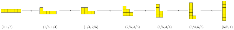
For a given slope vector , the ray is the set of triangular partitions having as an admissible slope vector, i.e.
(3.1)
This is an infinite chain in (see Figure 3.2). For instance, we have the ray
See also illustration in Figure 3.2. As any line of irrational slope contains at most one integral point, it follows that for all there is one and only one triangular partition of size on any ray associated to an irrational slope.
4. Triangular Dyck paths
Figure 4.1. The -Dyck path .
For a given triangular partition , we consider the set of -Dyck paths.
Observe that conjugation gives a bijection between and .
We further write , when , and say that its elements are
-Dyck paths. Observe that , for all and , since the corresponding triangular partitions coincide. It is often convenient to consider that partitions are padded with zero parts to make them of length .
As we have already mentioned, classical Dyck paths correspond to the case , with . For instance, we have the equivalent descriptions
As is very well known, these are counted by the Catalan numbers . In general, we set .
For integral partitions , the greatest common divisor plays an interesting role in our story. We have and , for coprime integers and . The cells of lying on its diagonal are of the form , with .
Figure 4.2. .
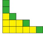
In preparation for upcoming notions, it will be interesting to consider the skew partition , in which stands for the partition obtained by adding one to each of the parts of including its zero parts. The above skew partition is readily seen to consist of “independant” columns, as illustrated in Figure 4.2 with .
The sequence of sizes of these columns is precisely . The choice of will depend on the context, and it will be larger than the number of parts of .
For a fixed , the -area (or simply area) of a -Dyck path is the number of cells lying in the skew shape . In terms of the -area sequence of , in which , we clearly have .
Definition 4.1.
For any subset of , we consider the -area:
Figure 4.3. A sim cell of relative to .
4.1. Similar cells (Diagonal inversions)
Let be a given triangular partition.
With the notations of Equation 1.2, for any consider the set of cells of that have hooks in that are “similar” to :
where .
The cardinality of this set, denoted by , is the similarity index888This just another name for the “dinv” statistic, that we choose to stress its natural geometrical meaning. of with respect to . Expressed in words, the similarity index of with respect to counts the number of cells of having “hook triangle slope vectors” compatible with the (average) slope vector of (represented by in Figure 1.2). Since at corner cells, we have and , we get
and . Hence, any corner cell of is always a -sim-cells, irrespective of .
The sim-cells of the partitions contained in are marked by stars in Figure 4.4.
Figure 4.4. Sim-cells for subpartitions of . The first 6 subpartitions are similar to .
The following is an example of a sequence of similar triangular partitions:
They all share the common slope vector .
Lemma 4.1(with B. Dequêne).
If is a triangular partition, then the subpartitions such that are exactly those that lie on the ray corresponding to the slope vector .
5. Counting -Dyck paths
The enumeration of triangular Dyck paths has an interesting (ongoing) history, which has up to now been restricted to the integral case. Even if the simple counting in the case of any integer pairs had already been worked out in the 1950s (see [8]), it is only rather recently that the overall enumerative combinatorics community has become aware of that fact. For a long time, only the “coprime case” was deemed really understood, recently going under the name of rational Catalan combinatorics.
These include the classical Fuss-Catalan numbers when (or equivalently when ). A direct extension of the classical “cycling” argument shows that, for and coprime integers, the number -Dyck paths is given by the formula
(5.1)
A formula for the non-coprime case of is described in the next subsection.
5.1. Bizley formula
In the general “integral” situation, the enumeration formula of -Dyck paths takes the form of a sum of terms indexed by partitions of the greatest common divisor of and . This is what makes it harder to “guess” a formula999Most guessing approaches rely (directly or indirectly) on the fact the numbers considered have nice factorization in small prime numbers., since the numbers obtained do not factor nicely in general, even if they are effectively sums of nicely factorized numbers. The Grossman-Bizley formula (see [8]) is:
(5.2)
where with and coprime, so that . It is worth recalling that is the number of size permutations of cycle type , with
where has parts of size .
Specific examples of Equation 5.2 are:
(5.3)
Observe that, for fixed coprime numbers and , all the formulas for , with , may be presented in the form of the generating function:
(5.4)
As it happens, this is a specialization of a more general formula (see Equation 7.5).
5.2. Explicit number of Dyck paths for all triangular partitions
For all triangular partitions of size at most , the number of -Dyck paths may be found in the Table 5.1. In the next subsection we will see how to calculate these numbers recursively.
Table 5.1. Number of -Dyck paths
5.3. General recursive formula for triangular partitions
For any partition triangular , the -area enumerator of -Dyck paths, is
(5.5)
Since conjugation is an area-preserving bijection between the set of -Dyck paths and the set of -Dyck paths, we clearly have . In preparation for the upcoming proposition, let us consider the following notions. The bounding word , of a partition , encodes the simplest southeast lattice path such that the cells of the diagram of are those that sit below . Thus ,
where , and , for . For two partitions and , we denote by the partition whose bounding word/path is the concatenation of words: . The empty partition acts as the identity for this associative product.
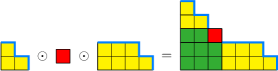
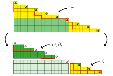
Three-way decompositions of the form , with indicating a one cell partition, will be of special interest. Observe that the middle one cell partition “” necessarily corresponds to a corner of . For example,
Figure 5.1. A decomposition .
Let us denote by the set of pairs corresponding to three-way decompositions of , of the form , with the corner cell sitting on the diagonal of . In formula,
(5.6)
Recall also that stands for the interior of , which is obtained by removing from all the cells on its diagonal.
Then, the number of -Dyck paths may efficiently be calculated with the following recursive formula.
Figure 5.2. First return cell , with marking other diagonal cells.
Proposition 5.1.
Denoting by the diagonal of a given triangular partition , then for the -area enumerator of -Dyck, we have the recurrence
(5.7)
with initial condition .
In particular, setting , we have
(5.8)
This is a direct generalization of the well-known classical recurrence for Dyck path. Its proof corresponds to a suitably adapted “first return to diagonal” argument typically used in the proof of the classical case (see Figure 5.2). It is noteworthy that all possible and that occur in the right-hand side of Equation 5.7 are triangular, as they are respectfully factors of and . Hence, for a given partition , the set of partitions that will arise in the recurrence can only be factors (for the -product) of partitions obtained by successive removal of diagonals. Hence, they all have a slope in common with that of .
The -area enumerators for all triangular partitions of size at most are as follows (avoiding repetitions for conjugate partitions):
5.4. Counting by Area and Sim
As in [9], we may consider the enumeration of -Dyck paths with respect to two statistics: “area” and “sim”, in the triangular case101010Our “sim” is the “dinv” of loc. cit.. The resulting -polynomials:
(5.9)
plays a central role in a wide range of subjects. Once again, applying conjugation to partitions contained in , it is easy to check that . It follows from 4.1 that, for any triangular partition of size , we have
(5.10)
where the remaining terms are of degree (strictly) less than . In the particular case , one may further see that
(5.11)
with the missing terms only involving Schur functions indexed by partitions having a second part larger or equal to . Taking into account the symmetry to avoid unnecessary repetitions, the values of for (all) triangular partitions of size at most are as given in Table 5.2. The entries are expressed in terms of Schur functions , so that the Schur positivity (see next section) of is made apparent.
Table 5.2. Table of values .
A constant term formula for is given in [9, Prop. 7.2.1]. It follows that is symmetric in and , even though this is not evident in Equation 5.9.
Setting , we often get nice product formulas. For instance,
In the case of , with and coprime integers, we have
(5.12)
For any triangular partition , with two parts, we further have
(5.13)
6. Generic Schur function expansion
The polynomials are not only symmetric, but extensive explicit calculations suggest that they always expand positively in the Schur polynomials basis. The following conjecture of [9, Conj. 7.1.1] is supported by extensive calculations (for all triangular partitions of ); and in some instances proofs and/or justifications via representation theory (see [6, 12]).
Conjecture 1.
For any triangular partition of size , the polynomial affords a positive Schur-expansion
(6.1)
The sum runs over (length ) partitions such that .
Specific values are:
(6.2)
whenever , and . These exhaust all possibilities for two part triangular partitions, since we must have if we want to be triangular. See [11, section 3]
6.1. Several parameters
Conjecturally, there is a natural extension of the previous Schur-expansions that encompass situations involving more parameters, hence involving Schur functions indexed by partitions having more than two parts. In some instances these are obtained as the -character of the -alternating component of representations of , as discussed in [7, 6, 5], thus explaining the Schur positivity. In the representation theoretic framework, one can show that these expressions become stable once . We may thus present them as positive integer coefficient linear combination of “formal” Schur expansions :
(6.3)
Writing for , we may summarize our theoretical and experimental observations about these as follows:
(1)
for all :
(6.4)
(2)
for all ,
(6.5)
(3)
if has more than parts, then ;
(4)
if , then ;
(5)
if , with triangular of length at most , then
(6.6)
(6)
for any ,
(6.7)
(7)
for all and such that , and , then
(6.8)
where the second summation runs over subsets of that satisfy the stated requirements.
To finish parsing the right-hand side of this last equality, we recall 4.1, and set
(6.9)
We underline that this right-hand side is exactly the combinatorial description of the coefficient of in the Delta theorem.
Extending this equality to any triangular partition would thus have an interesting impact on possible extensions of this theorem.
Besides cases already covered, some experimentally calculated values are as follows
Observe that one may “predict” the equality using Equation 6.5 in conjunction with Equation 6.6, since , , and is the conjugate of .
Observe in that some coefficients are larger than . Although these last values may be simply inferred just from the knowledge of Equation 6.8, they do agree with representation theoretic descriptions not discussed here. For more on this see [4].
6.2. Hook shape component.
A classical plethystic evaluation of Schur functions makes it easy to restrict a symmetric function to its “hook shape component”. Indeed, recall that
(6.10)
using Frobenius notation for hooks, and with standing for a “formal plethystic variable” such that . Then, it is easy to show that
In other words, the multiplicity of a hook indexed Schur function in is the coefficient of in Equation 6.11.
For instance, the above formula gives of the terms of , leaving only 21 terms to be explained:
The remaining terms may be obtained using Equation 6.8.
A striking fact is that essentially corresponds to the triply graded Poincaré series of the Khovanov-Rozansky homology of some torus knots, for adequate choices of .
7. Triangular parking functions
Figure 7.1. Parking function.
For any partition and , a height parking function of form is simply a standard tableau of shape . Observe that the skew-partition is a set of disjoint columns, say of respective size .
It follows readily that the number of standard tableaux considered is:
(7.1)
Observe also that the skew Schur function is equal to
(7.2)
Given a triangular partition and , the overall set -parking functions of height , is the set which we denote by .
For , with coprime integers, the total number of -parking functions (of height ) is well known to be equal to .
More generally, for with , such that coprime and , we also have a parking function analog of Equation 5.2:
(7.3)
7.1. Symmetric function counting
It is natural to extend the above enumeration to a symmetric function -enumeration of height parking functions, setting:
(7.4)
In the special cases , with coprime, there is (see [2, 3]) a symmetric function version of Equation 5.4:
(7.5)
We have the following nice extension of Equation 5.7 for the symmetric function enumeration of parking functions, whose proof follows a very similar argument.
Proposition 7.1.
For any triangular partition and any , the generic symmetric function enumerator of -parking functions satisfies the recurrence
(7.6)
with initial condition , and where the summation runs over the set of triples such that , with the partition corresponding to a cell of the diagonal of .
Formulas for a -enumeration of -parking functions with special values of may be found in [9]. One may extend these for general values of , and there are stable several parameter (i.e. ) extensions of the form:
which specialize at to the above mentionned -enumeration. This is ongoing work.
References
[1]
Drew Armstrong, Nicholas A. Loehr, and Gregory S. Warrington, Rational
parking functions and Catalan numbers, Annals of Combinatorics 20
(2016), no. 1, 21–58, https://doi.org/10.1007/s00026-015-0293-6.
[3]
Jean-Christophe Aval and François Bergeron, A note on: rectangular
Schröder parking functions combinatorics, Sém. Lothar. Combin.
79 ([2018–2020]), Art. B79a, 13,
https://arxiv.org/abs/arXiv:1603.09487.
[4]
François Bergeron, Multivariate diagonal coinvariant spaces for
complex reflection groups, Adv. Math. 239 (2013), 97–108,
https://doi.org/10.1016/j.aim.2013.02.013.
[5]
by same author, Open questions for operators related to rectangular Catalan
combinatorics, J. Comb. 8 (2017), no. 4, 673–703,
https://doi.org/10.4310/JOC.2017.v8.n4.a6.
[8]
M. T. L. Bizley, Derivation of a new formula for the number of minimal
lattice paths from to having just contacts with
the line and having no points above this line; and a proof of
Grossman’s formula for the number of paths which may touch but do not rise
above this line, J. Inst. Actuar. 80 (1954), 55–62.
[9]
Jonah Blasiak, Mark Haiman, Jennifer Morse, Anna Pun, and George H. Seelinger,
A shuffle theorem for paths under any line, 2021,
https://arxiv.org/abs/arXiv:2102.07931.
[10]
Sylvie Corteel, Gaël Rémond, Gilles Schaeffer, and Hugh Thomas,
The number of plane corner cuts, Adv. in Appl. Math. 23
(1999), no. 1, 49–53, https://doi.org/10.1006/aama.1999.0646.
[11]
Eugene Gorsky, Graham Hawkes, Anne Schilling, and Julianne Rainbolt,
Generalized -Catalan numbers, Algebr. Comb. 3
(2020), no. 4, 855–886, https://doi.org/10.5802/alco.120.
[12]
James Haglund, Jeffrey Brian Remmel, and Andrew Timothy Wilson, The
Delta conjecture, Trans. Amer. Math. Soc. 370 (2018), no. 6,
4029–4057, https://doi.org/10.1090/tran/7096.
[13]
M. Lothaire, Algebraic combinatorics on words, Encyclopedia of
Mathematics and its Applications, vol. 90, Cambridge University Press,
Cambridge, 2002, https://doi.org/10.1017/CBO9781107326019.
[14]
Irene Müller, Corner cuts and their polytopes, Beiträge Algebra
Geom. 44 (2003), no. 2, 323–333.

 , with
  marking other diagonal cells.