Resolvent estimates for one-dimensional Schrödinger operators with complex potentials
Abstract.
We study one-dimensional Schrödinger operators with unbounded complex potentials and derive asymptotic estimates for the norm of the resolvent, , as , separately considering and . In each case, our analysis yields an exact leading order term and an explicit remainder for and we show these estimates to be optimal. We also discuss several extensions of the main results, their interrelation with some aspects of semigroup theory and illustrate them with examples.
Key words and phrases:
Schrödinger operator, complex potential, pseudospectrum, resolvent estimate2010 Mathematics Subject Classification:
34L40, 35P20, 47A10, 81Q121. Introduction
The structure of the pseudospectrum of non-self-adjoint operators can be very non-trivial and in general unrelated to the location of the spectrum. This fact is well-known to be responsible for typical non-self-adjoint effects such as spectral instabilities or long-time semigroup bounds unrelated to the spectrum, see e.g. [37, 16, 17, 23] for details.
For Schrödinger operators with complex potentials , the pseudospectral analysis was initiated in the seminal paper of E. B. Davies, cf. [15], where lower estimates for the resolvent norm inside the numerical range of , , were obtained by a semi-classical pseudomode construction. The latter was subsequently generalised: in the semi-classical case in particular in [40, 18] and in the non-semi-classical one in [30, 4, 29, 20].
The upper estimates of the resolvent norm at the boundary of were first obtained by L. Boulton in [12] for the quadratic potential. This work was followed up with several semi-classical generalisations in particular in [32, 18, 11, 35, 8, 9, 24, 3] and also in [19] based on semigroup compactness or known behaviour of spectral projections.
In this paper, we study the behaviour of the resolvent norm at the boundary of for non-semi-classical one-dimensional Schrödinger operators acting in or in for a wide class of unbounded complex potentials ranging from iterated log functions to super-exponential ones (which are not accessible by previously used methods).
Our assumptions on are compatible with those in [30] where lower resolvent norm estimates inside were obtained. More precisely, restricting ourselves in this section to purely imaginary , we assume that is eventually increasing, unbounded at infinity and that the conditions (reflecting the growth of )
| (1.1) |
with some , are satisfied, see Assumption 3.1 for details. Moreover, the condition
| (1.2) |
is related to the separation property of the domain of , see Sub-section 3.1.1, and the quantity naturally enters the remainders in the derived asymptotic formulas (similarly to what happens e.g. for diverging eigenvalues in domain truncations in [33] or for asymptotics of eigenfunctions in [31]).
It was established in [30] that diverges as the spectral parameter goes to infinity along a set of admissible curves determined by the potential. In particular, for operators in the restriction on admissible curves is given by (with )
| (1.3) |
where is the turning point of , determined by , is as defined in (1.1) and is arbitrarily small. Except for the case of monomial potentials, where scaling can be used to rewrite in semi-classical form, it was left as an open question whether the restrictions (1.3) are optimal. Our main results allow us in particular to answer this question in the affirmative (with additional assumptions on for the second restriction in (1.3), see Subsection 5.2).
Our first result (Theorem 3.2), specialised for purely imaginary potentials here, provides a two-sided estimate for the norm of the resolvent along the imaginary axis for operators on the half-line and it includes an exact leading order term and an explicit remainder estimate. Namely,
| (1.4) |
where is the complex Airy operator in (see Sub-section 2.3). In Section 5, we further explain how these results extend to operators in as well as to multi-dimensional operators with radial potentials (see Sub-sections 5.3 and 5.5). Moreover, in Sub-section 5.6 we indicate how our strategy can be used in a semi-classical case where the problem substantially simplifies as only local properties of are needed (similarly to the pseudomode construction in [30]). In Sub-section 5.1, we extend Theorem 3.2 (with ) to describe the behaviour of the norm of the resolvent along general curves inside the numerical range
with . Precise resolvent estimates for semi-classical operators were found in [11]; in the special cases of the Davies operator and the imaginary cubic oscillator our construction allows us to recover those same curves (see the discussion for power-like potentials in Sub-section 7.1).
An analogous result (Theorem 4.2) is derived for operators in when for a smaller class of smooth, even, purely imaginary potentials satisfying and
-
\edefnn(i)
is eventually increasing:
-
\edefnn(ii)
is regularly varying:
where
-
\edefnn(iii)
has controlled derivatives:
Under these conditions the resolvent norm of the operator
satisfies
where is the generalised Airy operator
| (1.5) |
solves the equation and and are determined by
The additional smoothness and growth restrictions on for this result stem from employing pseudo-differential operator techniques. The regular variation assumption arises naturally due to scaling (similarly to the analysis of the eigenfunctions’ concentration in [31]). Basic properties of generalised Airy operators are described in Appendix A and a detailed spectral analysis can be found in [5], including precise resolvent norm estimates.
The result (1.4) in particular relates the behaviour of at infinity to the decay/growth of the resolvent along the imaginary axis, with the linear potential (i.e. the Airy operator) being the transition between the two cases. For sub-linear potentials, the resolvent norm diverges on the imaginary axis and the rate of divergence becomes very fast for slowly growing (e.g. iterated log) potentials (see Section 7 with several examples). The interest in such operators has been highlighted in recent research on one-parameter semigroups, e.g. [7, Thm. 1.5] relates the decay of solutions of the Cauchy problem to the growth of the resolvent norm along the imaginary axis. More precisely, if is the generator of the bounded -semigroup and , then for fixed we have
For more general rates, see [36]. Inspired by the open problem presented by C. Batty [6], we note that Theorem 3.2 enables us to characterise the class of rates (e.g. ) for which we can construct potentials such that the resolvent norm of the corresponding Schrödinger operator equals that given rate (see Section 6 for details).
The proof of Theorem 3.2, originally inspired by [23, Prop. 14.13], revolves around a separate analysis of depending on whether or not is contained in a neighbourhood of the turning point designed so that is approximately constant inside. More specifically, the proof consists of the following steps (several technical extensions are additionally needed for the case of potentials with non-zero real part).
- \edefnn(1)
-
\edefnn(2)
In Proposition 3.4, in a neighbourhood of (see (3.18)), appropriately shifted and scaled, we Taylor-approximate with the complex Airy operator to yield
as . The norm resolvent convergence of (a localised realisation of) to the complex Airy operator follows from the second resolvent identity and it makes use of certain graph-norm estimates introduced in Subsection 2.3.
-
\edefnn(3)
In Proposition 3.5, we show that our estimate for the norm of the resolvent of cannot be improved by finding functions such that as
The proof relies on exploiting the localisation technique used in step 2 and the fact that the operators involved have compact resolvent. Thus the norms of those resolvents can be obtained from the appropriate singular values and the corresponding eigenfunctions are used to find the family.
-
\edefnn(4)
We combine the results from the previous steps with the aid of certain commutator estimates and a suitably constructed partition of unity.
The proof of Theorem 4.2, which describes the asymptotic behaviour of the resolvent norm along the real axis, follows the template outlined above but on the Fourier side and with substantial modifications at several stages. In particular, the commutator estimates in Step 4 are obtained using pseudo-differential operator techniques (see Lemma 4.4) resulting in additional smoothness and regularity assumptions.
The remainder of our paper is structured as follows. Section 2 introduces our notation and recalls some fundamental facts for the various tools used throughout (Fourier transform, pseudo-differential operators, Schrödinger operators with complex potentials, Airy operators and functions of regular variation). In Section 3 we formulate and prove Theorem 3.2 for the resolvent norm in . Section 4 is devoted to the proof of Theorem 4.2 for the resolvent norm in the real line. Section 5 includes further extensions of the main theorems, in particular the resolvent estimates on more general curves in the numerical range. In Section 6 we deal with the inverse problem mentioned above and Section 7 illustrates our results on some concrete potentials. Finally, in Appendix A we show the key properties of the first order generalised Airy operators used in the proof of Theorem 4.2.
2. Notation and preliminaries
We write , , , and . The characteristic function of a set is denoted by , the -norm by , the other norms by , the space of smooth functions of compact support by and the Schwartz space of smooth rapidly decreasing functions by . The commutator of two operators , is denoted by . For a multi-index , we write .
In the one-dimensional setting, we will refer to the first and second order differential operators with and , respectively, reserving the symbols and for statements in higher dimensions.
If denotes a Hilbert space, we shall use and to represent the inner product and norm on that space. The inner product shall be denoted by , or just by if there is no ambiguity, and the norm by or just by . The other norms will be represented by with denoting the space of essentially bounded functions endowed with the essential norm .
Let be open, and . We will denote the Sobolev spaces by and (the latter representing as usual the closure of in , see e.g. [21, Sub-sec. V.3] for definitions). We shall generally be concerned with the particular cases where , and .
If is a bounded operator on a Banach space , we will denote by its spectral radius, i.e. with denoting the spectrum of . As usual, will denote the set of eigenvalues of and its resolvent set.
If , , , are closed linear operators on the Banach space , we say that converges to in the norm resolvent (or generalised) sense, and we write , if there exists such that , for some , and as (refer to [27, Sub-sec IV.2.6] for a detailed exposition of the concept).
If and are two linear operators acting in the Hilbert space , we say that is an extension of , and write , if and for all . Note that our notation covers the case , i.e. the extension does not have to be proper.
To avoid introducing multiple constants whose exact value is inessential for our purposes, we write to indicate that, given , there exists a constant , independent of any relevant variable or parameter, such that . The relation is defined analogously whereas means that and .
2.1. Fourier transform and pseudo-differential operators
For , the Fourier and inverse Fourier transforms read (with )
we also use , and retain the same notations to refer to the corresponding isometric extensions to .
We recall that the Schwartz space, , is endowed with the family of semi-norms
When introducing pseudo-differential operators in Section 4, we follow [1, Part I]. Given , the symbol class is the vector space of smooth functions such that for any there exists satisfying
| (2.1) |
This space is endowed with a natural family of semi-norms defined by
| (2.2) |
Furthermore, for , the space of amplitudes consists of the smooth functions such that for any there exists satisfying
| (2.3) |
This space is endowed with the family of semi-norms
| (2.4) |
We associate a pseudo-differential operator with the symbol via
and it can be shown that this is a bounded mapping on (see [1, Thm. 3.6]).
2.2. Schrödinger operators with complex potentials
Let be open. For a measurable function , we denote the maximal domain of the multiplication operator determined by the function as
| (2.5) |
the Dirichlet Laplacian in is denoted by and
| (2.6) |
Suppose that the complex potential , , satisfies a.e. in , , and, with ,
| (2.7) |
Under these assumptions on one can find the (Dirichlet) m-accretive realization by appealing to a generalised Lax-Milgram theorem [2, Thm. 2.2]. It is also known that the domain and the graph norm of separate, i.e. and
| (2.8) |
Furthermore,
| (2.9) |
is a core of . For details see [2, 28, 33] and [13, 26], [21, Chap. VI.2] for cases with a minimal regularity of .
2.3. Airy operators
An important class of objects in our analysis are complex Airy operators; details on the claims summarised here can be found in [23, Ch. 14] and in Section A of this paper for the more general case.
The rotated Airy operator in with and is denoted by
| (2.10) |
It is well-known that has compact resolvent, its spectrum is empty, its adjoint satisfies and
| (2.11) |
Moreover, since , we also have
| (2.12) |
In Section 4, we use operators in of type (with )
| (2.13) |
which we refer to as generalised Airy operators (on Fourier space). The motivation for this choice of terminology is as follows. By transforming the complex Airy operator, , to Fourier space (via , where denotes the Fourier transform, see Sub-section 2.1), one obtains . Operators of type extend the simple structure of . Many properties of the usual complex Airy operators are preserved for . Namely, has compact resolvent, empty spectrum,
| (2.14) |
and
| (2.15) | ||||
It is in fact possible to carry out this extension further to operators with much more general . See Appendix A for details and [5] for resolvent estimates.
2.4. Regular variation
A continuous function satisfying
| (2.16) |
is called regularly varying (at infinity) and is called the index of regular variation. We can rewrite as
| (2.17) |
where is a slowly varying function, i.e.
| (2.18) |
It is known (see [34, Sec. 1.5]) that, if is slowly varying, then
| (2.19) |
and that the convergence in (2.18) is locally uniform in (see [34, Thm. 1.1]). Moreover, a representation theorem (see [34, Thm. 1.2]) states that
| (2.20) |
where is positive and measurable, is continuous and
| (2.21) |
In this paper, we shall be chiefly concerned with functions with index .
3. The norm of the resolvent in the range of
3.1. Assumptions and statement of the result
We begin by describing the class of potentials encompassed by our estimate for the norm of the resolvent.
Assumption 3.1.
Suppose that for some . With and , assume further that a.e. in and that the following conditions are satisfied:
-
\edefnn(i)
is unbounded and eventually increasing:
(3.1) -
\edefnn(ii)
has controlled derivatives: there exists such that
(3.2) -
\edefnn(iii)
we have:
(3.3) -
\edefnn(iv)
is sufficiently small w.r.t. :
(3.4)
For a potential satisfying Assumption 3.1, the Schrödinger operator in
| (3.5) |
is specified as in Sub-section 2.2; see also our comments in Sub-section 3.1.1 below.
To state our result, we introduce
| (3.6) |
with as in (3.4). Assuming that is sufficiently large, we denote by the unique solution (see (3.1)) to the equation
| (3.7) |
(sometimes called a turning point of ) and define
| (3.8) | ||||||
Furthermore, noting that by Assumption i and (3.7) we have as , then from Assumption iv we deduce that
| (3.9) |
Theorem 3.2.
3.1.1. Remarks on the assumptions
Firstly, potentials satisfying Assumption 3.1 obey the separation condition (2.7). To see this, consider a cut-off function with and such that on . We decompose as , where , and . Thus it suffices to verify that (2.7) holds for large . By Assumptions 3.1 iv, ii and iii, we get for
| (3.11) |
3.2. Proof of Theorem 3.2
With as in (3.8), let
| (3.13) |
The proof is structured in four steps. Firstly, we prove the claim ”away” from the zero of . Then we study the behaviour of the norm of the resolvent locally (i.e. near ). Next we establish a lower bound for the norm. Our final step, the theorem proof proper, combines the previously derived estimates. Throughout the proof we are chiefly concerned with the behaviour as and will therefore assume to be as large as needed for our assumptions to hold without further comment.
Let
| (3.14) |
where will be specified in Proposition 3.4 and (see Assumption 3.1 ii). By remarks in Sub-section 3.1.1, the above choice for the width of implies that is approximately equal to inside that interval (see (3.12)) and this fact will be used in the proofs below.
From (3.14) and the already noted fact that as , we deduce
| (3.15) |
In what follows, we shall assume to be large enough so that and . This ensures that .
3.2.1. Step 1: estimate outside the neighbourhood of
Proposition 3.3.
Proof.
Define and note that and . Let such that , then
Therefore
| (3.16) |
Next we find a lower bound for in . By Assumption 3.1 i, is unbounded and increasing in and, since it is also bounded on , we have for large enough and
Applying the mean-value theorem for the first term inside the with and noting secondly that by (3.14) and therefore by (3.12), we deduce that for
A similar result can be found for . Therefore
| (3.17) |
Hence by combining (3.17) and (3.16) we conclude that for all with
as required. ∎
3.2.2. Step 2: estimate near
Proposition 3.4.
Proof.
If , the Taylor expansion of around yields
where . Let
| (3.19) |
and consider the operator in
Given , we define a unitary operator on by , . Then for any
If and , then
where and , are as defined in (3.8). We are now in a position to define the value of for the remainder of the proof
| (3.20) |
Let us denote
| (3.21) |
then
| (3.22) |
For any by (3.14) and hence , i.e. . Combining this fact with (3.12), we deduce
For all we have and therefore
| (3.23) |
Let be the operator in
| (3.24) |
Our next aim is to prove that as with from the statement of Theorem 3.2.
We begin by showing that there exists such that . Note that and, from (3.23), we have
| (3.25) |
as . Note also that it follows from (2.11) that
| (3.26) |
in the estimate of the second term we use the fact that is bounded and therefore from the property of adjoint , if is densely defined, we get that has a bounded extension. Hence, using (3.26) and (3.25), we obtain
It therefore follows from (3.9) and an appropriate choice of sufficiently small (independent of ) that, for all large enough , the operator is invertible and
| (3.27) |
This shows that indeed , as claimed.
Furthermore, using (3.26) and (3.27) we deduce
| (3.28) |
We now prove that as . Using the second resolvent identity, (3.22), (3.26), (3.28) and (3.23), we obtain
| (3.29) | ||||
We therefore conclude that
| (3.30) |
But and hence there exists such that for all
Let and such that . Then and (we view a function from as belonging to using the natural embedding). Finally, with , we conclude that
3.2.3. Step 3: lower estimate
Proposition 3.5.
Proof.
We retain the notation introduced in the proof of Proposition 3.4; in particular, and is as defined in (3.24).
With a sufficiently large , the operators , , on , are compact, self-adjoint and non-negative. Let and let be a corresponding normalised eigenfunction, i.e. , and . Note that and it is straightforward to verify that
| (3.31) |
Moreover, from (3.29), we obtain
| (3.32) |
Note also that arguing as in the justification of (3.28) and recalling (2.12), we obtain
| (3.33) |
Since , we have
| (3.36) |
The last two terms can be estimated using (3.31), (3.32), (3.33), (3.34) and (3.35)
| (3.37) | ||||
as . Hence as . Similarly, writing , we obtain as . Thus using (3.32), we arrive at
Recalling from the proof of Proposition 3.4 that and letting , then with and we conclude
from which the claim follows. ∎
3.2.4. Step 4: combining the estimates
Lemma 3.6.
Proof.
Let , then
and hence
| (3.41) |
Let , , as in the proof of Proposition 3.3. Repeating the above calculations, we deduce
| (3.42) |
By Assumptions 3.1 iv and i, there exists such that
| (3.43) |
Moreover, from (3.15), for sufficiently large . Consequently applying (3.43) and Assumption 3.1 i
Combining this last finding with (3.41) and (3.42)
and therefore for any
where we have applied (3.38). Choosing a sufficiently small and using Assumption 3.1 iii we deduce
Finally, applying once more Assumption 3.1 iii
as claimed. ∎
4. The norm of the resolvent in the real axis
4.1. Assumptions and statement of results
We begin by describing the class of potentials covered by our estimate for the norm of the resolvent in the real axis.
Assumption 4.1.
Suppose that with satisfying
-
\edefnn(i)
is even:
(4.1) -
\edefnn(ii)
is eventually increasing:
(4.2) -
\edefnn(iii)
is regularly varying:
(4.3) where
(4.4) -
\edefnn(iv)
has controlled derivatives:
(4.5)
For potentials satisfying Assumption 4.1, we consider the Schrödinger operator
| (4.6) |
as in Sub-section 2.2.
To state the result, we define the positive real numbers via the equation
| (4.7) |
notice that is eventually increasing by Assumption (4.2), thus is well-defined for all sufficiently large . Moreover, it follows that as . Finally, let
| (4.8) |
Lemma 4.7 shows that as .
Theorem 4.2.
4.1.1. Remarks on the assumptions
Moreover, by Assumption 4.1 iv with , for any arbitrarily small
and it follows that satisfies condition (2.7). Hence the graph norm of separates
| (4.12) |
Finally, the following estimates for the derivatives of shall be used in Steps 2 and 3 of the proof of Theorem 4.2.
Lemma 4.3.
4.2. Proof of Theorem 4.2
We transform the problem to Fourier space and implement there the strategy of Sub-section 3.2. To this end, we introduce the operators in
| (4.14) | ||||||
Notice that , for all and for all . Thus the separation of the graph norm of , see (4.12), yields
| (4.15) |
The proof has an analogous structure to that of Theorem 3.2 but nonetheless some steps are more technical. In particular, our simple estimate of the commutator of and a cut-off partition of unity in Step 4 of Theorem 3.2 (see Sub-section 3.2.4) requires more effort here (see Step 0 below).
4.2.1. Step 0: commutator estimate
The proof of our next lemma specialises that of [1, Thm. 3.15] for the operators that we are interested in.
Lemma 4.4.
Let and be such that
| (4.16) |
and let be such that is bounded. For and , we define the operators (with and )
| (4.17) |
Then, for any , we have
| (4.18) |
where is a pseudodifferential operator with symbol
| (4.19) |
Moreover, for every with , there exist and , independent of and , such that
| (4.20) |
Proof.
Let and , then our hypotheses ensure and . Moreover (with )
and therefore both symbols define continuous mappings on (see [1, Thm. 3.6]). An analogous claim holds for , , . Furthermore, by the composition theorem [1, Thm. 3.16], is a pseudo-differential operator with symbol determined by
where for any and (with )
| (4.21) | ||||
| (4.22) |
Thus the composition formula (4.18) follows by simple manipulations.
In the following, and , are arbitrary. We define with given by (4.22). Using the assumption (4.16), we obtain
| (4.23) | ||||
where in the last step we have used the fact
Notice that is independent of and and therefore (4.23) shows that . Applying Fubini’s theorem for oscillatory integrals [1, Thm. 3.13] to (4.21), we deduce that for any and
Moreover, by Peetre’s inequality (see [1, Lem. 3.7])
Therefore (4.23) also implies that, for any , w.r.t. and, for any , there exists such that
| (4.24) |
Hence by [1, Thm. 3.9], for a sufficiently large (depending on )
| (4.25) | ||||
with independent of and . Since , it follows that, for any , and , and therefore
is well-defined. Moreover, by (4.25), for large enough and some (independent of and )
Hence
| (4.26) |
and
The claim (4.20) follows by Young’s inequality and (4.26). ∎
4.2.2. Step 1: estimate outside the neighbourhoods of
Proposition 4.5.
Proof.
In what follows, we shall assume to be large and positive. Let with and consider
Note that
appealing to Assumption 4.1 iv with for the last estimate. Furthermore, for any , there exist such that
Noting also that, for any , there exists such that
Hence, with an appropriate choice of , we conclude that there exists such that
| (4.30) |
which proves the claim. ∎
4.2.3. Step 2: estimate near
We start with three lemmas used in the proof of Proposition 4.9 below.
Proof.
Because of Assumption 4.1 i, it suffices to consider . Assume firstly that and let be the slowly varying function such that (see (2.17)–(2.18)). Then for all
and the claim follows by the locally uniform convergence for (see Sub-section 2.4).
For , let be arbitrarily small and take such that for any . If is as in Assumption 4.1 ii, then, for any and , we have
where we have used the assumption that is increasing in . Therefore, by (4.11) and Assumption 4.1 iii, there exists such that
Hence
If , then we use the first part of the proof to find such that
which concludes the proof for . ∎
Proof.
By Assumption 4.1 i, it is enough to consider what happens to
Let , then there exists such that
| (4.31) |
Let be the slowly varying function such that (see (2.17)–(2.18)) and consider . Using the representation of in (2.20) and properties of and (see (2.21)), there exists such that for all and , we have
| (4.32) |
Therefore by (2.17)
| (4.33) |
and we conclude that there exists such that
| (4.34) |
Combining (4.31) and (4.34), we find that
| (4.35) |
Notice that for any and
| (4.36) |
We now apply Lemma 4.6 to to deduce that there exists such that
| (4.37) |
which, in conjunction with (4.35) and (4.36), yields the desired claim. ∎
Lemma 4.8.
Proof.
First observe that (4.5) with and (4.11) imply that
| (4.40) |
and therefore for every and all sufficiently large
| (4.41) |
Hence for every , .
Next, consider , such that on and denote . We split as and show that is uniformly bounded and satisfies (A.11) uniformly in . The claims then follow from Proposition A.2.
Firstly, by the locally uniform convergence of to (see Lemma 4.6)
| (4.42) |
Secondly,
| (4.43) |
since is bounded and converges to locally uniformly. Moreover the last term in (4.43) is estimated using (4.13) with and the fact that is outside . Thus altogether we obtain
| (4.44) |
thus (A.11) is indeed satisfied (uniformly for all sufficiently large ). ∎
Proposition 4.9.
Proof.
We shall derive estimate (4.46) for such that . The procedure when is similar (see our comments at the end of the proof).
Clearly and we introduce
With as in (4.14), let us define the following operator in
Given to be chosen below, we define a unitary operator on by
Then with
| (4.47) |
In what follows, we select as , where is defined by equation (4.7), i.e. , and we recall that as . We denote
| (4.48) |
and, from (4.48) and , we obtain
| (4.49) |
We further denote
| (4.50) | ||||
where (with an abuse of notation) and from Lemma 4.8. Our next aim is to show that
| (4.51) |
converges to in the norm resolvent sense as .
The spectra of and , and hence those of and , are empty, see Lemma 4.8 and Proposition A.1. Moreover
| (4.52) |
Take and define
| (4.53) | ||||
Then
with and . From the graph norm estimates (4.39) and (2.15), we obtain
Therefore, with from (4.8) and ,
Hence by Lemma 4.7, the density of in and a standard resolvent identity argument, see e.g. the proof of [14, Lem. 2.6.1], we arrive at (employing (4.52))
| (4.54) |
as . We transport the graph-norm estimate (4.39) to the Fourier side
| (4.55) |
and thus in particular (similarly as in the justification of (3.26))
| (4.56) |
It follows, by choosing a sufficiently small , independently of , that the bounded operator is invertible, for all large enough , and
| (4.57) |
This shows that for and furthermore, using (4.56), we deduce
| (4.58) |
By the second resolvent identity, we have as
where, for the last estimate, we have applied (4.56) and (4.58). Thus from (4.54) and (4.49), we find
| (4.59) | ||||
For the case , we repeat the above arguments but defining instead , , and . ∎
4.2.4. Step 3: lower estimate
Proposition 4.10.
Proof.
We retain the notation introduced in the proof of Proposition 4.9; in particular, and from (4.51). The proof follows the steps of that of Proposition 3.5.
Consider , , on and such that
| (4.63) |
with and sufficiently large (see the statement of Lemma 4.4 and, in particular, (4.20)). Recall that as (see (4.7)), hence pointwise in as .
Next, we justify that and therefore . Similarly to (4.32)–(4.33) (but estimating instead an upper bound), and using the locally uniform convergence of to (see Lemma 4.6), we find that , , with any arbitrarily small , for all sufficiently large . Moreover, as in the proof of Lemma 4.8, consider , such that on and denote . Then the estimate (4.13) and Leibniz rule show that there exist , independent of , such that for all sufficiently large ,
| (4.64) |
Thus for sufficiently large , satisfies the assumptions of Lemma 4.4 (with constants independent of ). Hence, for all , we have
| (4.65) |
and, using (4.64), (4.18), (4.19) and (4.20),
with independent of . Hence by (4.63)
| (4.66) |
Since converges to uniformly on bounded sets (see Lemma 4.6), we have
| (4.67) |
Moreover, is a core for and we conclude that is relatively bounded w.r.t. . Hence we have indeed .
Next, we write
| (4.68) | ||||
and we proceed to estimate all the above terms but the first one. Employing (4.62), (4.58) as well as the graph norm separation as in (4.55) for (and analogously for the adjoint ), we obtain as
in the last two estimates we have also used (4.66) and (4.67), respectively. Since furthermore , then
For , we have
where in the last step we use , and
For and , we define and we fix some . Then
Since , we conclude that
For the second term, we use the facts that , and , with . Then, by the Hausdorff-Young inequality (see e.g. [22, Prop. 2.2.16]), we have that , with . Thus we find
where in the last step we have applied Hölder’s inequality with . Hence when we have
4.2.5. Step 4: combining the estimates
With , and from (4.27), (4.45), let , , be such that
| (4.70) |
with and sufficiently large (see the statement of Lemma 4.4 and, in particular, (4.20)), and define
| (4.71) |
Lemma 4.11.
Let satisfy Assumption 4.1 with and let , with arbitrarily small, and . Then for any and
| (4.72) |
Proof.
Lemma 4.12.
Proof.
Let , then
| (4.76) |
(see (4.15) and (4.28)). Note also that
| (4.77) |
Furthermore, by Assumption 4.1 iii, and recalling our earlier remarks on regularly varying functions, in particular (2.17) and (2.19), we obtain from (4.7)
| (4.78) |
for any arbitrarily small and any sufficiently large .
In the case , appealing to (4.18), (4.20) and (4.70) and noting that are bounded operators for (recall Assumption 4.1 iv), we have for any
Moreover, using (4.5), (4.77), and the fact that as
Since , we have applying (4.30)
and, since as (see (4.7) and (4.11)), we conclude
Furthermore, by (4.18), (4.20), (4.5), (4.77) and
Hence
| (4.79) |
and
| (4.80) |
as claimed. Moreover, using (4.7) and (4.11)
For , applying (4.18) we obtain
| (4.81) |
In order to estimate , we introduce cut-off functions , , , satisfying
| (4.82) | ||||
with . Then applying Lemma 4.11 and Young’s inequality for products (note that ) and using the fact that as
| (4.83) | ||||
Since , using (4.30) we have
Applying (4.18) to and using (4.82) and the fact that, by (4.5) and (4.76), for any , we obtain
| (4.84) | ||||
Furthermore, noting firstly that and secondly that, for sufficiently small , as (see (4.7) and (4.78)), we have by (4.72), (4.76) and Young’s inequality for products
which yields
| (4.85) |
Moreover, repeating the same arguments which we have used for , we find
| (4.86) | ||||
Returning to (4.83) with (4.85) and (4.86) and noting that for any small but fixed we can always find such that
we obtain
| (4.87) | ||||
Next we estimate the second term in the right-hand side of (4.81) using (4.70), (4.72), (4.76), , Young’s inequality for products and as
| (4.88) | ||||
Combining (4.81), (4.87) and (4.88), we have
as required. Finally, using (4.7) and (4.78)
since can be chosen arbitrarily small. This concludes the proof. ∎
Lemma 4.13.
Proof.
Let and with . Applying (4.18) with and , we have for
with
and as in (4.19), (4.21) and (4.22). Noting that and , and consequently in , we get
Hence
| (4.90) | ||||
Applying (4.20) and (4.70) and recalling , we find for and . Moreover
| (4.91) |
for . The second and higher order terms in the right-hand side of the above inequality have already been estimated in Lemma 4.12 (see (4.79), (4.80), (4.87) and (4.88)); we have for and any arbitrarily small
We proceed to estimate the first term in the right-hand side of (4.90) as
using the fact that as in the last step. A similar estimate can be derived for . Applying both of them and in (4.90) yields the desired result. ∎
Proof of Theorem 4.2.
Let and let us write , where with and as in (4.71). Then we have
and therefore, noting that and using Lemma 4.12, we obtain as
| (4.92) | ||||
with small and as in (4.74).
Firstly, note that and and therefore . Moreover, by Proposition 4.9 and Lemma 4.13, as
| (4.93) | ||||
Thus by (4.92), (4.7) and Lemma 4.7, we have as
| (4.94) |
Combining (4.94) and (4.95), we find that as
Using (4.75), we arrive at
| (4.96) |
Since is a core for and, equivalently, for , we can extend the above estimate to any using a standard approximation argument. The proof of the theorem follows by an appeal to Proposition 4.10 and the use of the inverse Fourier transform to take the result back to -space. ∎
5. Extensions and further remarks
5.1. The norm of the resolvent inside the numerical range
A simple application of the triangle inequality allows us to obtain estimates for the resolvent norm in regions adjacent to the imaginary and real axes as well as to include further bounded perturbations.
In particular, for as in Section 3 with purely imaginary satisfying Assumption 3.1, Theorem 3.2 and (5.1) with , , yield
| (5.2) |
as . Thus assuming that does not grow too slowly (e.g. is bounded below by a strictly positive constant), that is large enough and that are sufficiently small, the region in the first quadrant of (which contains the numerical range of the operator and its spectrum, if any) determined by
| (5.3) |
with , is non-empty and unbounded. Moreover, the resolvent satisfies inside this region.
For as in Section 4, one obtains from Theorem 4.2 and (5.1) with , , , that
| (5.4) |
as . Thus the resolvent satisfies for
| (5.5) |
In both cases, bounded perturbations can be included in an analogous way.
5.1.1. The norm of the resolvent along curves adjacent to the imaginary axis
A more precise examination of the proof of Theorem 3.2 reveals that it is in fact possible to estimate along curves
| (5.6) |
even outside the region determined by (5.3). Let for simplicity obey Assumption 3.1 and, with and as defined in (3.20) and in Assumption 3.1 iii, respectively, let satisfy
| (5.7) |
where (with )
| (5.8) |
In our analysis, we shall be mainly concerned with two types of curves:
-
\edefnn(1)
with for , corresponding asymptotically to the critical region (5.3), i.e. where satisfies
(5.9) -
\edefnn(2)
with , , and therefore grows away from the critical region, i.e. where satisfies
(5.10)
Note that, in the first case, we have due to the fact that is bounded on compact sets in and therefore, by Assumption 3.1 iii, condition (5.7) holds automatically.
We further observe that, for any , it can be shown that (see [23, Sec. 14.3.1]) and that there exists a precise asymptotic estimate for (see [11, Cor. 1.4])
| (5.11) | ||||
For any , applying standard arguments it is also possible to extend the graph-norm estimate (2.11)
| (5.12) |
and to deduce from this (see e.g. (3.26), (3.33))
| (5.13) | ||||
Proposition 5.1.
Sketch of proof.
We shall sketch the proof of this result by closely following the steps in Sub-section 3.2, keeping the notation introduced there but omitting details whenever the arguments used earlier remain valid.
Step 1
Repeating the reasoning in Proposition 3.3 (replacing with ), we find that for all such that
| (5.15) |
Step 2
With and as in Proposition 3.4, it is clear that (recall )
| (5.16) |
We shall prove next that as . For any , the operator is bounded and invertible and moreover by (5.13) we have
| (5.17) |
Recalling from Proposition 3.4 that for large enough and defining , we find
Moreover, by (5.17), (3.29) and (5.7), we have
It follows that is invertible and as . Since , we conclude that for , as claimed. Moreover, and, using (3.28), (3.33) and (5.17), we deduce as
| (5.18) |
Furthermore, we have
| (5.19) | ||||
Hence
and therefore by (3.29) and (5.17) and using the fact that satisfies (5.9) or (5.10)
It follows that
| (5.20) |
and hence from (5.16) as
Arguing as in the last stage of Proposition 3.4, this yields as
| (5.21) | ||||
Step 3
We follow the proof of Proposition 3.5, replacing with , to find such that
Moreover, with , we have (see (5.20))
| (5.22) |
Recalling the cut-off functions , we write
and, applying (5.18) and (5.22) (refer also to (3.34) and (3.35)), we deduce
as . Hence, noting that is bounded below by a positive constant when , we have
Similarly as and consequently
As before, we set . Then and
| (5.23) |
Step 4
Repeating the commutator calculations in the proof of Lemma 3.6 for , we find for all and
which we use to estimate (with small and )
Hence
Then for any , , we have for
and therefore as
We conclude this subsection with a general construction for the level curves of the resolvent (some examples will be shown in Section 7). Letting , we note (see (5.11)) that as , i.e. when lies outside the region (5.3). Applying (5.11) again, we find
The above equation can be rewritten as
where is the Lambert function that solves for . Although cannot be written in terms of elementary functions, the following bounds have been found for (see [25, Thm. 2.7])
and thus we deduce
| (5.24) |
From (5.14), we have and hence
Substituting , with , we obtain
| (5.25) |
We remark that as expected formula (5.25) indicates that the level curves of a sub-linear potential (where as ) will cross the imaginary axis into . We also note that, when (i.e. is the Davies operator), then and the above equation becomes
(compare these curves with (7.4) for and with the known formulas derived in [11, Prop. 4.6]).
5.1.2. The norm of the resolvent along curves adjacent to the real axis
We can similarly estimate , for as in (4.6) and potential satisfying Assumption 4.1, along general curves adjacent to the real axis
| (5.26) |
with satisfying
| (5.27) | |||
| (5.28) |
where
, and , and are as defined in (2.13), (4.8) and (4.10), respectively. We are interested in two types of curves:
-
\edefnn(1)
with for , corresponding asymptotically to the critical region (5.5), i.e. where satisfies
(5.29) -
\edefnn(2)
with , , and therefore grows away from the critical region, i.e. where satisfies
(5.30)
Note that, in the first type above, we have due to the fact that is bounded on compact sets in and therefore, by Lemma 4.7 and the fact that as , condition (5.28) holds automatically.
In [5, Ex. 4.3], the following asymptotic estimate was found
| (5.31) |
Before formulating our result, we also note that, for any , it is possible to extend the graph-norm estimates (A.14) applying standard arguments to
| (5.32) |
and it follows (see e.g. (3.26), (3.33), (4.56))
| (5.33) | ||||
Proposition 5.2.
Sketch of proof.
We shall sketch the proof of this result by closely following the steps in Sub-section 4.2, keeping the notation introduced there but omitting details whenever the arguments used earlier remain valid. We introduce the operators (refer also to (4.14) and (4.28))
| (5.35) |
Step 1
Repeating the reasoning in Proposition 4.5 (replacing with ) and applying (4.30), we find that for all such that (with arbitrarily small and some )
| (5.36) | ||||
using assumption (5.27) in the last step. This proves that (4.29) continues to hold when we replace with .
Step 2
We retain the notation in Proposition 4.9. From (4.47), (4.48) and (4.51), we have
| (5.37) |
Our next aim is to prove that as . To do this, we argue as in Step 2 of Proposition 5.1. For any , the operator is bounded and invertible and moreover by (5.33) we have
| (5.38) |
Recalling from Proposition 4.9 that for large enough and defining , we find
Moreover, by (4.59), (5.38) and (5.28), we have
It follows that is invertible and as . Since , we conclude that for , as claimed. Moreover, and, using (4.58) and (5.38), we deduce as
| (5.39) |
Furthermore, we have (see the argument in (5.19))
Hence
and therefore by (4.59) and (5.38) and using the fact that satisfies (5.29) or (5.30)
It follows that
| (5.40) |
and hence from (5.37) and (5.40) as
Arguing as in the last stage of Proposition 4.9, this yields as
| (5.41) | ||||
Step 3
We follow the proof of Proposition 4.10, replacing with , to find such that
| (5.42) |
Moreover, with , we have (see (5.40))
| (5.43) |
Recalling the cut-off functions , we write
| (5.44) | ||||
and we proceed to estimate the terms in the right-hand side, except the first one, as we did in Proposition 4.10. Applying (5.39), (5.42) and (5.43), we have as
| (5.45) | ||||
From the proof of Proposition 4.10, the fact that for large enough (refer to Step 2 above, noting also (5.38)), (5.42) and (5.43), we find as
| (5.46) | ||||
Using again the proof of Proposition 4.10, estimate (4.58) and the above arguments, we have as
| (5.47) | ||||
To estimate the last term in the right-hand side of (5.44), we adapt the corresponding section of the proof of Proposition 4.10.
| (5.48) |
For , using (4.55) and arguing as in (5.46), we have as
For , using , estimating each term in turn as in the proof of Proposition 4.10 and then proceeding as in the case, we obtain as
Hence, going back to (5.48), we have as
| (5.49) |
and therefore, returning to (5.44) with the individual term estimates, we obtain
| (5.50) |
Writing , we deduce that as (see (5.47)) and hence, applying (5.50) and (5.43), we arrive at
Recalling that (see (5.37)) and letting , then with . It follows
and hence
| (5.51) |
Step 4
We begin by updating the commutator estimate (4.73) provided in Lemma 4.12. Starting with (4.76) and applying (5.35) followed by (5.27), we find
| (5.52) |
Furthermore
| (5.53) |
As in the proof of Lemma 4.12, we consider firstly the case . The initial commutator estimate remains valid
| (5.54) |
Turning to the first term in the right-hand side and applying (4.5) with , (5.53), (5.36) from Step 1, (5.27) and the fact that as
Furthermore using (4.18), (4.5) with and (5.53), we have
Hence
and, returning to (5.54), this yields the estimate
We already established that as . Moreover by (5.28)
We note that estimate (4.77) plays no role in the proof of Lemma 4.12 for the case . On the other hand, estimate (4.76) is indeed used but its replacement here (5.52) is simply a matter of substituting with ; the same substitution happens between (4.30) (from Proposition 4.5), which is also used in Lemma 4.12 when , and (5.36) (Step 1 above). We can therefore repeat the proof for to derive
Combining both cases, we have
where for any arbitrarily small
| (5.55) |
Moreover
| (5.56) |
We also need to revise estimate (4.89) in Lemma 4.13. We repeat the original argument, with instead of , to arrive at (4.90). Taking in (4.70), we have for and . Moreover, expanding as in (4.91) and using our new commutator estimates, we have for any arbitrarily small and
We can now estimate the first term in the right-hand side of (4.90) as
where in the last step we have used the fact that as we have
(refer back to the definition (5.55)). We can similarly estimate the other terms in the right-hand side of (4.90) to find as
| (5.57) | ||||
We conclude this sub-section with a general construction for the level curves of the resolvent similar to that in Sub-section 5.1.1 but considering now those adjacent to the real axis. Letting , we re-write (5.31) as
This is an equation in which we can solve using the Lambert function (refer to Sub-section 5.1.1 for further details)
to deduce
Using (5.34) and substituting , with , we obtain (recall )
| (5.61) |
Finally, we note that, when (i.e. is the Davies operator), then and the above equation becomes
| (5.62) |
(compare these curves with (7.5) for and with the known formulas derived in [11, Prop. 4.6]).
5.2. Optimality of the pseudomode construction in [30]
In this paper, the curves in along which the norm of the resolvent diverges are found by a non-semi-classical pseudomode construction. As a corollary of (5.3), using Assumption 3.1 ii, we find that for any , the norm of the resolvent is uniformly bounded inside the region determined by . This shows that the lower edge (i.e. the left-hand side) of the condition [30, Eq. (5.5)] is optimal.
Similarly using (5.5) we obtain optimality of the upper edge of the condition [30, Eq. (5.5)] (with . Denoting the regular variation index of by , we obtain from (4.7) and (2.17) that
| (5.63) |
Hence, recalling that as and using (2.19), we get (with any )
| (5.64) |
Similarly from we arrive at (with any )
| (5.65) |
Then, using (5.63), inequality (5.5) can be rewritten as (the constant can be given explicitly)
| (5.66) |
Finally, employing (5.63), (5.64) and (5.65), the condition (5.66) is satisfied if with some which complements [30, Eq. (5.5)].
5.3. Extension of Theorem 3.2 to operators in
We outline a procedure to extend Theorem 3.2 to operators defined on the real line.
Assumption 5.3.
Suppose that with , for some and let , . Assume further that the following conditions are satisfied:
-
\edefnn(i)
is unbounded and eventually increasing (in )/decreasing (in ):
-
\edefnn(ii)
has controlled derivatives: there exist such that
-
\edefnn(iii)
grows sufficiently fast: we have
where
(5.67)
With satisfying Assumption 5.3, we consider the Schrödinger operator
| (5.68) |
in (refer to Sub-section 2.2 for details). Moreover, for sufficiently large , we define the turning points by
| (5.69) |
In the following, we use the notation , .
Proposition 5.4.
Sketch of proof.
To justify the above claim, we introduce a partition of unity. For , , with large enough so that and , let , , satisfying
For convenience, we shall denote , , and . For , we write , with , , and introduce the operators in
Since satisfies Assumption 3.1 and , we have by (3.48)
| (5.71) |
Moreover, with the isometry in , it is easy to see
| (5.72) |
Since and in , by combining (5.71) and (5.72) we find
and therefore
| (5.73) |
Since , then arguing as in Proposition 3.3 we deduce that for large enough
It follows that for and sufficiently large
reasoning as in the proof of Proposition 3.3 and applying Assumption 5.3 ii. Hence
| (5.74) |
Our strategy to prove Theorem 3.2 can be re-deployed, with minimal and obvious changes, when Assumption 5.3 i is replaced with
and , , to prove that as
| (5.77) |
where we have used the fact that and therefore . One can analogously treat the case where the potential is bounded on one of the half-lines and unbounded on the other one.
5.4. Extension of Theorem 4.2 to operators in
We briefly indicate how Theorem 4.2 can be adapted for operators in subject to a Dirichlet boundary condition at and with satisfying the conditions in Assumption 4.1 for . The even extension of to , and the corresponding complex potential , satisfy Assumption 4.1 up to a possible lack of smoothness at , which can however be removed by a compactly supported perturbation , similarly as in Subsection 5.1. Then Theorem 4.2 can be applied to in . Since the odd extension of each belongs to and for each odd , we have , we arrive at the desired inequality for any (see (4.96) in the proof of Theorem 4.2)
5.5. Extension of Theorem 3.2 to radial operators
Let and consider the Schrödinger operator in with
| (5.79) |
We justify below that the claim of Theorem 3.2 remains valid in this case; a relatively small real part of the potential (in the sense of Assumption 3.1) can be added in a straightforward way but we omit the details.
Proposition 5.5.
Sketch of proof.
The first step of the proof (see Sub-section 3.2.1) can be performed in the same way using the multidimensional operator , i.e. we split into , with , and the rest.
In the second step (see Sub-section 3.2.2), we decompose in a standard way into a countable family (labelled by ) of one-dimensional operators in
| (5.81) |
with appropriate domains (see e.g. [39, Chap. 18] for details)). The challenge is to obtain suitable estimates for all and all with independent of .
Following the same procedure (in particular shift and scaling and using the fact that ) as in Sub-section 3.2.2, we arrive at operators in
| (5.82) |
where , ,
| (5.83) |
with (see (3.21)) and
| (5.84) |
Note that for a fixed , as and that for all ( can be set to 0 for and to 1 for ) and all large .
An important observation is that the graph norm of satisfies (uniformly for all and all large )
| (5.85) |
To see this, it is enough to note
and to apply (2.11). This equation also shows that for and hence
| (5.86) |
Furthermore, since as and is bounded on bounded sets in , we can find (independent of ) such that for all we have . It follows from (5.86) that for all and all . Note that this last estimate combined with (5.85) implies that for all and all .
The estimates of (see (3.23)) remain valid and we have (uniformly in )
| (5.87) |
as . Thus
| (5.88) |
is invertible and its graph norm is equivalent to that of (uniformly in ). Moreover, by the second resolvent identity, the previous estimates and (3.23), we obtain (uniformly in )
Since for all and all large and is m-accretive, we get
| (5.89) |
for finitely many , , the same claim follows by treating as a perturbation. The rest of the proof of this step is the same as the one in Sub-section 3.2.2 and can be reformulated as an estimate for the full operator .
The third step (see Sub-section 3.2.3) can be performed for with a fixed and so it requires only minor and straightforward adjustments.
The last step (see Sub-section 3.2.4) is completely analogous. ∎
5.6. Remarks on semi-classical operators
We indicate how the strategy of Theorem 3.2 applies in the semi-classical case for the operator in subject to Dirichlet boundary condition at with and , noting that resolvent norm bounds for semi-classical Schrödinger operators with purely imaginary potential have been derived in e.g. [32, 18, 11, 35, 8, 9, 24, 3]. We assume that satisfies the conditions in Sub-section 2.2 so that is m-accretive. Suppose in addition that is such that and there is such that
| (5.90) | ||||
We focus on the resolvent estimate for the spectral point from the range of the potential.
In Step 1 (see Sub-section 3.2.1), one considers functions with with a suitably selected as . Then the quadratic form estimate (see Proposition 3.3), Taylor’s theorem and (5.90) yield (for the considered functions )
| (5.91) |
In Step 2 (see Sub-section 3.2.2), for functions supported in , taking out the factor , the shift , rescaling and Taylor’s theorem lead to operators in
| (5.92) |
Selecting so that , we obtain
| (5.93) |
where as . Hence choosing with , we readily obtain the norm resolvent convergence to the Airy operator , with and , see Sub-section 2.3,
| (5.94) |
Thus, rewritting (5.94) for , we arrive at (for the considered functions )
| (5.95) |
6. An inverse problem
In [7, Thm. 1.5], the authors relate the rate of time-decay of the norm of a one-parameter semigroup to the rate of growth of the norm of the resolvent of its generator along the positive part of the imaginary axis. Inspired by the presentation on this topic in [6], we consider the following problem. Which assumptions must a non-negative, unbounded function satisfy for there to exist a potential such that the Schrödinger operator verifies as ? Theorem 3.2 enables us to answer this question as follows.
Proposition 6.1.
Proof.
Note that (6.4) can be indeed solved as the left-hand side is an increasing function in . It is immediate that determined by (6.4) satisfies (6.5). Moreover such is unbounded and increasing. It remains to verify Assumptions 3.1 ii and iii. Firstly, by differentiating (6.4) and employing (6.1), we have
Similarly using (6.1) and (6.2)
Lastly, by (6.3)
As for the second statement in the Proposition, let be regularly varying with index (see Sub-section 2.4) and eventually increasing and assume furthermore that it satisfies (6.6). From the facts that is bounded on compact subsets of and that it is eventually increasing, we have as
Moreover, using (6.6) and the previous estimate,
Finally, calling and arguing as in Lemma 4.6, it is possible to show that as , and we have
for , as required. ∎
Example 6.2.
Example 6.3.
We remark that conditions (6.1)–(6.3) include many others rates, growing both faster (e.g. with ) and more slowly (e.g. or ). For instance, consider with . The condition (6.1) is satisfied for any increasing . To verify (6.2), observe that integration by parts yields, as
| (6.7) |
Hence
| (6.8) |
Finally, since
| (6.9) |
for the condition (6.3) we arrive at
| (6.10) |
7. Examples
We illustrate the behaviour of the norm of the resolvent in several examples where the numerical range, , and the spectrum, if any, lie in the first quadrant of the complex plane. In the sequel we denote
Recall that we have , , thus we focus on the behavior of for in the first quadrant only.
7.1. Power-like potentials
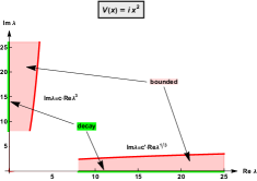
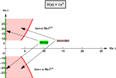
Let , , with . It is routine to verify that the assumptions of Theorems 3.2 and 4.2 (see also the extensions in Sub-sections 5.3, 5.4) are satisfied and we thus have
| (7.1) | ||||
with the Airy operators and (see (2.10) and (2.13), respectively) and
note that, in this example, the remainder for is dominated by which is independent of .
For , , we find similar formulas with improved remainder term for the real axis (in this case, and moreover we can take in (4.9))
| (7.2) | ||||
We can also derive estimates for odd potentials , , along both the positive and negative parts of the imaginary axis (see (5.77) in our closing remarks in Sub-section 5.3), namely as ,
| (7.3) |
From (7.1), we note that, for power-like potentials with degree , decays progressively faster as with limit , the decay rate for . As we consider potentials that grow super-exponentially, the asymptotic behaviour of changes, and an additional factor (a negative power of ) comes into play (see Example 7.3). At the other end of the range for , as , , we observe the growth rate of along the imaginary axis increasing ever faster. The transition from power-like potentials to (more slowly growing) logarithmic ones also determines a change in asymptotics for , with growth along the imaginary axis becoming exponential (see Example 7.2).
Arguing as in the closing remarks in Sub-section 5.1.1 (see (5.25)), we find the level curves for the resolvent of with potential , . Note that and hence
| (7.4) |
Since we require , we need , and, for , we must have .
We can similarly find the level curves, adjacent to the real axis, for the resolvent of with even potential , (refer to Sub-section 5.1.2). Note that and hence an application of (5.61) yields
| (7.5) |
Noting that , as , and therefore any even monomial is admissible as a potential in this instance.
Two cases of particular interest are the operators with potentials (the Davies operator) and (the imaginary cubic oscillator). They have been studied in detail in the literature using both semi-classical and non-semi-classical methods: see e.g. [15, 12, 18, 11, 30] for the Davies example and [10, 11, 35, 19] for the cubic case. The behaviour of the norm of the resolvent for each of them is illustrated in Fig. 7.1 which shows the regions of uniform boundedness of described in Sub-section 5.1 (see (5.3) and (5.5)). Furthermore we observe that the level curves determined by (7.4) with and match those found using semi-classical methods in [11, Prop. 4.6, Prop. 4.2] and that, as expected, the level curves determined by (7.4) with and those determined by (7.5) with (see (5.62)) are symmetrical with respect to the bi-sector .
7.2. Slowly growing potential
Let with domain . Then
As in the sub-linear potential case, the fact that grows along the imaginary axis leads to an -shifted critical curve that intersects it at some .
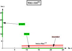
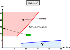
7.3. Fast growing potential
Let with . Then
| (7.6) |
which is as before illustrated in Fig. 7.1. Since the decay of on the imaginary axis is faster than for any polynomial potential, the region for uniform boundedness of adjacent to the imaginary axis is correspondingly wider. Note that Theorem 4.2 on the behaviour of for is not applicable in this case, see also Figure 7.1, and therefore the description of the critical region next to the real axis is currently an open question although [30, Eq. (5.5)] provides a clue as to what it may look like.
Appendix A Generalised Airy operator
We analyse the following first order operator in which we refer to as a generalised Airy operator
| (A.1) |
Proposition A.1.
Let with a.e. and let be as in (A.1). Then
-
\edefitn\selectfonti)
is densely defined and m-accretive;
-
\edefitn\selectfonti)
has a compact resolvent if
(A.2) -
\edefitn\selectfonti)
the adjoint operator reads
(A.3) -
\edefitn\selectfonti)
we have
(A.4) hence if
(A.5)
Proof.
-
\edefnn\selectfonti)
It is clear that and therefore that is densely defined. Moreover, a standard cut-off argument, using a sequence for and any , see e.g. [28, Lem. 3.6], shows that
(A.6) is a core of . Thus for all , we have , hence
i.e. is accretive; moreover,
(A.7) For and , we have
(A.8) thus
(A.9) This shows that is injective, that is bounded and that . Moreover, is closed.
Next we show that is dense in . Let and assume that for some , . Elementary calculations show that
solves . Furthermore, since and
hence . We have thus shown , consequently , and therefore is m-accretive.
- \edefnn\selectfonti)
-
\edefnn\selectfonti)
By simple adjustments of the arguments to prove 1, we can show that with the maximal domain is m-accretive. Moreover, for all and , we have
which shows that . However, the fact that is m-accretive implies that is also m-accretive (see e.g. [21, Thm. 6.6]) and therefore it must be the case that , as claimed.
- \edefnn\selectfonti)
A.1. Separation property
Under more restrictive assumptions on , analogous to (2.7), the graph norm of separates.
Proposition A.2.
Let , with some , satisfying a.e., and suppose that
-
\edefitn(i)
there exist and such that
(A.11) -
\edefitn(ii)
is relatively bounded w.r.t. , i.e. there is such that
(A.12)
Then
| (A.13) |
and we have
| (A.14) | ||||
the constants depend only on , , and .
Proof.
Consider such that and on . We split , where , and . Since and , the assumption (A.11) is satisfied also for , possibly with a different constant .
Let be the operator determined by (A.1) with potential . We show that the separation (A.13) and (A.14) holds for . The latter remain valid for since is bounded.
For , see (A.6) and (A.13), integration by parts yields
Using (A.11) for (see remarks above), Young inequality with and the assumption (A.12) in the second step, we arrive at
We select so that , thus . Therefore for all (and hence for all )
| (A.15) |
Since the opposite inequality is immediate, we conclude with (A.13) for and hence for since is bounded. The reasoning for is completely analogous. ∎
References
- [1] Abels, H. Pseudodifferential and Singular Integral Operators. De Gruyter, 2011.
- [2] Almog, Y., and Helffer, B. On the spectrum of non-selfadjoint Schrödinger operators with compact resolvent. Comm. Partial Differential Equations 40 (2015), 1441–1466.
- [3] Almog, Y., and Henry, R. Spectral analysis of a complex Schrödinger operator in the semiclassical limit. SIAM J. Math. Anal. 48 (2016), 2962–2993.
- [4] Arifoski, A., and Siegl, P. Pseudospectra of damped wave equation with unbounded damping. SIAM J. Math. Anal. 52 (2020), 1343–1362.
- [5] Arnal, A., and Siegl, P. Generalised Airy Operators. arXiv preprint arXiv:2208.14389 (2022).
- [6] Batty, C. Rates of decay associated with operator semigroups. Talk at the CIRM conference Mathematical aspects of the physics with non-self-adjoint operators: 10 years after, Feb. 2021., 2021.
- [7] Batty, C. J., Borichev, A., and Tomilov, Y. -tauberian theorems and -rates for energy decay. J. Funct. Anal. 270 (2016), 1153–1201.
- [8] Bellis, B. Subelliptic resolvent estimates for non-self-adjoint semiclassical Schrödinger operators. J. Spectr. Theory 9 (2018), 171–194.
- [9] Bellis, B., and Hitrik, M. Semigroup expansions for non-selfadjoint Schrödinger operators. J. Funct. Anal. 277 (2019), 3586–3598.
- [10] Bender, C. M., and Boettcher, S. Real Spectra in Non-Hermitian Hamiltonians Having Symmetry. Phys. Rev. Lett. 80 (1998), 5243–5246.
- [11] Bordeaux Montrieux, W. Estimation de résolvante et construction de quasimode près du bord du pseudospectre. arXiv:1301.3102, 2013.
- [12] Boulton, L. Non-self-adjoint harmonic oscillator, compact semigroups and pseudospectra. J. Operator Theory 47, 2 (2002), 413–429.
- [13] Brézis, H., and Kato, T. Remarks on the Schrödinger operator with singular complex potentials. J. Math. Pures Appl. 58 (1979), 137–151.
- [14] Davies, E. B. Spectral theory and differential operators. Cambridge University Press, 1995.
- [15] Davies, E. B. Semi-Classical States for Non-Self-Adjoint Schrödinger Operators. Comm. Math. Phys. 200 (1999), 35–41.
- [16] Davies, E. B. Pseudospectra of differential operators. J. Operator Theory 43 (2000), 243–262.
- [17] Davies, E. B. Linear operators and their spectra. Cambridge University Press, 2007.
- [18] Dencker, N., Sjöstrand, J., and Zworski, M. Pseudospectra of semiclassical (pseudo-) differential operators. Commun. Pure Appl. Math. 57 (2004), 384–415.
- [19] Dondl, P. W., Dorey, P., and Rösler, F. A Bound on the Pseudospectrum for a Class of Non-normal Schrödinger Operators. Applied Mathematics Research eXpress (2016).
- [20] Duc, T. N. Pseudomodes for biharmonic operators with complex potentials. arXiv:2201.03305v1 [math.SP], Jan. 2022.
- [21] Edmunds, D. E., and Evans, W. D. Spectral Theory and Differential Operators. Oxford University Press, New York, 1987.
- [22] Grafakos, L. Classical Fourier analysis, vol. 249. Springer, New York, 2014.
- [23] Helffer, B. Spectral theory and its applications. Cambridge University Press, 2013.
- [24] Henry, R. On the semi-classical analysis of Schrödinger operators with purely imaginary electric potentials in a bounded domain. arXiv:1405.6183, 2014.
- [25] Hoorfar, A., and Hassani, M. Inequalities on the Lambert function and hyperpower function. J. Inequal. Pure and Appl. Math 9 (2008), 5–9.
- [26] Kato, T. On some Schrödinger operators with a singular complex potential. Ann. Scuola Norm. Super. Pisa, Cl. Sci. IV 5 (1978), 105–114.
- [27] Kato, T. Perturbation theory for linear operators. Springer-Verlag, Berlin, 1995.
- [28] Krejčiřík, D., Raymond, N., Royer, J., and Siegl, P. Non-accretive Schrödinger operators and exponential decay of their eigenfunctions. Israel J. Math. 221 (2017), 779–802.
- [29] Krejčiřík, D., and Nguyen Duc, T. Pseudomodes for non-self-adjoint Dirac operators. J. Funct. Anal. 282, 12 (2022), 109440.
- [30] Krejčiřík, D., and Siegl, P. Pseudomodes for Schrödinger operators with complex potentials. J. Funct. Anal. 276 (2019), 2856–2900.
- [31] Mityagin, B., Siegl, P., and Viola, J. Concentration of eigenfunctions of Schrödinger operators. J. Fourier Anal. Appl. 28 (2022).
- [32] Pravda-Starov, K. A Complete Study of the Pseudo-Spectrum for the Rotated Harmonic Oscillator. J. London Math. Soc. 73 (2006), 745–761.
- [33] Semorádová, I., and Siegl, P. Diverging eigenvalues in domain truncations of Schrödinger operators with complex potentials. SIAM J. Math. Anal. (to appear).
- [34] Seneta, E. Regularly varying functions. Springer-Verlag, Berlin-New York, 1976.
- [35] Sjöstrand, J. Resolvent Estimates for Non-Selfadjoint Operators via Semigroups. In Around the Research of Vladimir Maz’ya III. Springer New York, 2009, pp. 359–384.
- [36] Stahn, R. Decay of -semigroups and local decay of waves on even (and odd) dimensional exterior domains. J. Evolution Equations 18, 4 (2018), 1633–1674.
- [37] Trefethen, L. N., and Embree, M. Spectra and Pseudospectra: The Behavior of Nonnormal Matrices and Operators. Princeton University Press, 2005.
- [38] Tumanov, S. Completeness theorem for the system of eigenfunctions of the complex Schrödinger operator . J. Funct. Anal. 280 (2021), 108820.
- [39] Weidmann, J. Lineare Operatoren in Hilberträumen. Vieweg+Teubner Verlag, 2003.
- [40] Zworski, M. A remark on a paper of E. B. Davies. Proc. Amer. Math. Soc. 129 (2001), 2955–2957.