Self-Contrastive Learning based Semi-Supervised Radio Modulation Classification
Abstract
This paper presents a semi-supervised learning framework that is new in being designed for automatic modulation classification (AMC). By carefully utilizing unlabeled signal data with a self-supervised contrastive-learning pre-training step, our framework achieves higher performance given smaller amounts of labeled data, thereby largely reducing the labeling burden of deep learning. We evaluate the performance of our semi-supervised framework on a public dataset. The evaluation results demonstrate that our semi-supervised approach significantly outperforms supervised frameworks thereby substantially enhancing our ability to train deep neural networks for automatic modulation classification in a manner that leverages unlabeled data.
Index Terms:
Self-Supervised Learning, Semi-Supervised Learning, Automatic Modulation ClassificationI Introduction
Automatically recognizing or classifying the radio modulation is a key step for many commercial and military applications, such as dynamic spectrum access, radio fault detection, and unauthorized signal detection in battlefield scenarios. The modulation classification problem has gotten widely studied in the past few years. Two general types of algorithms, likelihood-based (LB) and feature-based (FB), have been applied to solve the modulation classification problem. Likelihood-based methods [1, 2] make decisions based on the likelihood of the radio signal and achieve optimal performance in the Bayesian sense. However, they suffer from high computational complexity. Feature-based methods [3, 4, 5], on the other hand, make decision based on the manually-extracted features from the radio signal. Given the input radio signal, various features related to phase, amplitude or frequency are manually extracted and then used as inputs of the classification algorithms. Machine learning algorithms, such as support vector machine (SVM) and decision trees, are popular candidates for the classification algorithms.
Recently, with advances in deep learning techniques, deep neural networks achieves a great success in multiple fields, such as image classification [6] and natural language processing [7]. Deep neural network models, such as convolutional neural networks (CNNs) [8, 9] and recurrent neural networks (RNNs) [10, 11], have also been applied to the modulation classification problem. Such neural network models directly feed the raw signal data or its transforms as input and generally achieve much better performance than previous approaches.
However, training a deep neural network model requires a large amount of training data. In practice, it’s usually difficult to collect a large volume of high quality and reliable radio signals as well as their modulations (labels) as training data. One common way to deal with the lack of training data is data augmentation. Previous studies proposed several data augmentation strategies [12, 13, 14] to avoid overfitting caused by the lack of training data. Another way is to utilize unlabeled data. The difficulty in collecting a large training dataset for radio modulation classification mainly comes from the labeling burden for radio signals. It is much eaiser to collect the radio signals without labeling them. Hence, it would help a lot if we could efficiently utilize unlabeled radio signals. As far as we know, the benefits of using unlabeled data have not yet been studied for the modulation classification problem.
Self-supervised learning, as a kind of unsupervised learning, obviates much of the labeling burden by extracting information from unlabeled data. Self-supervised learning algorithms have had great success in areas of computer vision [15], natural language processing [7], and IoT applications [16]. The goal of self-supervised learning is to train an encoder to extract useful intrinsic information (or features) from unlabeled data and use that information as the inputs to a classifier or predictor in a downstream task. Since these features already store a lot of intrinsic information about the original input, a simple classifier (e.g., linear) is enough for the downstream task. Using this approach, most training uses unlabled data to learn the instrinsic features. Only a small amount of labeled data is then needed to train the downstream classifier.
In this paper, we build a Semi-supervised Automatic Modulation Classification framework, namely, SemiAMC, to efficiently utilize unlabeled radio signals. SemiAMC consists of two parts: (i) self-supervised contrastive pre-training and a (ii) downstream classifier. In self-supervised contrastive pre-training, we apply the design of SimCLR [15], which is an effective self-supervised contrastive learning framework, to train an encoder using a large amount of unlabeled training data as well as data augmentation. Then, we freeze the parameters of the encoder and train a classifier, which takes the representations (output of the encoder) as input, based on a small amount of labeled training data.
We evaluate the performance of SemiAMC on a widely-used modulation classification dataset RadioML2016.10a[17]. The evaluation results demonstrate that SemiAMC efficiently utilizes unlabeled training data to improve classification accuracy. Compared with previous supervised neural network models, our approach achieves a better accuracy given the same number of labeled training samples.
II Related Work
In this section, we briefly introduce related background on automatic modulation classification, self-supervised and semi-supervised learning techniques.
II-A Deep Learning in Automatic Modulation Classification
Motivated by the success of deep learning techniques in computer vision [6] and NLP [7], deep neural network models, such as CNN [8], ResNet [9], and LSTM [10] have been applied to the automatic modulation classification task. Such neural network models directly take radio signals as input and predict the type of modulation as output. To further improve the performance of automatic modulation recognition, specific characteristics of the modulated radio signals are considered. For example, Zeng et al. [18] use spectrograms, generated from the radio signals through short-time discrete Fourier transform, as the input to a CNN classifier. Perenda et al. [19] separate the amplitude and phase series of the input and train based on a parallel fusion method. Most of the previous works focused on designing supervised models while we design a semi-supervised learning framework in this paper.
II-B Semi-Supervised Learning
Semi-supervised learning is a learning paradigm that leverages both labeled and unlabeled data to train machine learning models. With the development of deep learning techniques, deep neural network models become deeper and deeper and we need more and more labeled data to train such models. However, the collection of large datasets is very costly and time-consuming as it requires a lot of human labor work to annotate the dataset. In order to reduce the data labeling burden, a lot of semi-supervised learning algorithms [20] have been designed to make use of large number of unlabeled data as well as a small number of labeled data. In this paper, our semi-supervised approach is based on self-supervised contrastive learning, which has gotten great success in computer vision area. To our best knowledge, we are the first who apply self-supervised contrastive learning to automatic modulation classification problem.
II-C Self-Supervised Learning
Self-supervised learning is a learning paradigm where the model is trained on unlabeled data. Self-supervised contrastive learning is an typical self-supervised learning algorithm and has achieved outstanding performance [15]. The supervision of self-supervised contrastive learning comes from the user-designed pretext tasks which generate locally distorted data samples. A loss function can thus be generated that prefers mapping such similar inputs to nearby locations in the latent space.
Self-supervised learning can be used as the pre-training step in the semi-supervised learning algorithms [15, 16]. An encoder that collects intrinsic information from the original input (and maps it to a latent space) is trained with a self-supervised learning algorithm based on large amounts of unlabeled data. A small amount of labeled data can then be used to train a model on these features.
III Approach
In this part, we first introduce the signal model we consider in this paper. Then, we describe the design of SemiAMC.
III-A Signal Model
We consider a single-input single-output communication system where we sample the in-phase and quadrature components of a radio signal through an analog to digital converter. The received radio signal can be represented as
| (1) |
where refers to the modulated signal from the transmitter, refers to the path loss or gain term on the signal, and is the Gaussian noise. The received radio signal is sampled times at some sampling rate to obtain a length vector of complex values. In this paper, we treat the complex valued input as a 2-dimensional real-valued input. We denote it as , where is a matrix containing the in-phase (I) and quadrature (Q) components of the received signal samples.
The goal of this paper is to determine the modulation type for any given radio signal .
III-B Overview of SemiAMC
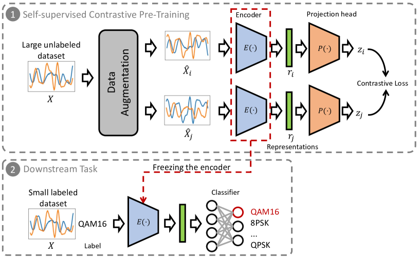
SemiAMC aims at training a classifier to accurately recognize the modulation type for any given radio signal. As a semi-supervised framework, SemiAMC is trained with both labeled and unlabeled data. We show the architecture of SemiAMC in Figure 1. The illustrated workflow is as follows.
The first step is called self-supervised contrastive pre-training, where we train an encoder to map the original radio measurements into low-dimensional representations. This is done in a self-supervised manner, with unlabeled data only. The supervision here comes from optimizing the contrastive loss function, that maximizes the agreement between the representations of differently augmented views for the same data sample.
In step two, we freeze the encoder learned during the self-supervised contrastive pre-training step, and map the labeled input radio signals to their corresponding representations in the low-dimensional space. The classifier can be trained based on these representations and their corresponding labels. Here a relatively simple classifier (e.g., linear model) usually work well, because the latent representation has already extracted the intrinsic information from the signal input. In this way, a small number of labeled data samples is enough to train the classifier. When we have enough labeled data, we can also fine-tune the last one or more layers of the encoder to further improve the performance of SemiAMC.
III-C Self-supervised Contrastive Pre-training
We apply SimCLR [15] as our self-supervised contrastive pre-training framework. As shown in Figure 1, our self-supervised contrastive pre-training mainly consists of four components.
III-C1 Data Augmentation
The first component is a stochastic data augmentation module. Given any signal input , two views of , that are denoted as and , are generated from the same family of data augmentation operations. The data augmentation algorithms are highly application dependent. For example, in image related applications, random color distortion, cropping, and Gaussian blue are commonly used data augmentation algorithms. In our approach, we augment the I/Q signal with the rotation operation [12] which could keep the features for classification. For a modulated signal , where and refer to vectors storing the in-phase (I) and quadrature (Q) signals, we rotate it with an angle randomly selected from . The augmented signal sample is
| (2) |
III-C2 Encoder
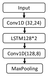
The second part is a neural network based encoder that extracts intrinsic information from the augmented examples and , and stores them in the latent representations and :
| (3) |
Various choices of the network architectures can be used to design the encoder. For example, CNN-based encoders are widely utilized in learning representations of visual data and RNN-based encoders are usually utilized to deal with time-series. Figure 2 shows the architecture of the encoder we use in our approach. The I/Q signal input is first passed through a 1D convolutional layer (32 kernels with size 24) to extract the spatial characteristics. The following two LSTM layers (with 128 units) are used to extract the temporal characteristics. In the end, the 1D convolutional layer (128 kernels with size 8) and the max pooling layer are used to generate the representations.
III-C3 Projection Head
The third part is a small neural network projection head that maps representations to the space where contrastive loss is applied. In our approach, we use a multilayer perceptron (MLP) with one hidden layer as the projection head, which means
| (4) |
where is the ReLU activation function. It has been proved that calculating the contrastive loss on ’s (instead of on the representations directly) improves the performance of self-supervised contrastive learning [15].
III-C4 Contrastive Loss
The last part is the contrastive loss function that is defined for a contrastive prediction task aiming at maximizing the agreement between examples augmented from the same signal input. We use the normalized temperature-scaled cross entropy loss (NT-Xent) [21] as the loss function. For a given mini-batch of examples in the training process, since for each example , we will generate a pair of augmented examples, there will be data points. The two augmented versions and of the same input are called a positive pair. All remaining in this batch are negative examples to them. Cosine similarity is utilized to measure the similarity between two augmented examples and . The similarity is calculated on and :
| (5) |
Here, refers to the norm of . The loss function for a positive pair of examples is defined as
| (6) |
where refers to the temperature parameter of softmax and is an indicator function equaling to 1 iff . The loss for all positive pairs is calculated and the average is used as the final contrastive loss.
IV Evaluation
In this section, we evaluate the performance of SemiAMC using a public dataset, RadioML2016.10a [17]. We first introduce the dataset we use and then show the experimental setup, including data preprocessing and detailed implementation. Finally, we analyze the performance of SemiAMC.
IV-A Dataset
We use RadioML2016.10a to study the performance of SemiAMC. RadioML2016.10a is a synthetic dataset including radio signals of different modulations at varying signal-to-noise ratios (SNRs). It consists of 11 commonly used modulations (8 digital and 3 analog): WBFM, AM-DSB, AM-SSB, BPSK, CPFSK, GFSK, 4-PAM, 16-QAM, 64-QAM, QPSK, and 8PSK. For each modulation, there are 20 different SNRs from dB to dB and there are 1000 signals under each SNR. Hence, the RadioML2016.10a has signal examples in total. Each signal in RadioML2016.10a has 128 I/Q samples. In our approach, we put each signal in a matrix .
IV-B Experimental Setup
We split the dataset into three parts: training, validation, and testing by a ratio of 2:1:1. Specifically, for each modulation type and SNR, we randomly divide the 1000 signals into 500 signals for training, 250 signals for validation, and 250 signals for testing. Normalized signals are used as the input.
In the self-supervised contrastive pre-training part, we use a two-layer projection head. The first layer is a fully connected layer with 128 hidden units and ReLU activation. The second is a fully connected layer with 64 hidden units without an activation function. The encoder, the output of which is 128, is trained under a batch size of 512, with a total of 100 batches, and initial learning rate with cosine decay. In the downstream task part, we freeze the encoder and build a two-layer classifier on the representations. The first layer of the classifier is a fully connected layer with 128 neurons and ReLU activation. The second is a Softmax layer with 11 neurons, one for each modulation scheme. We apply droupout and L2 regularization to mitigate over-fitting.
We first study the performance when all the training and validation data have labels. We then study the performance when only part of the training and validation data have labels. We also study the performance of our approach when different amounts of unlabeled data are used to train the encoder. We further compute the classification accuracy separately for each SNR and modulation scheme. We run five times with different random seeds and take the average as the final performance.

IV-C Comparison with Supervised Frameworks
In this part, we compare the performance of our semi-supervised learning framework to that of previous supervised frameworks when we have enough labeled training data. Specifically, here we assume that we have labels for all the training and validation data. We first train the encoder with all signal samples in the training dataset. Then, we freeze the encoder and train the classifier based on both of the signals and labels in the training set. During this process, we also fine-tune the parameters of the encoder to get better result. We stop the training process when the validation loss does not decrease for 30 epochs and use the model with minimum validation loss to predict the classification accuracy on test set.
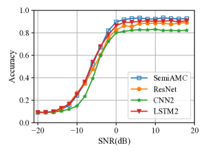
We compare the performance of SemiAMC against three supervised algorithms named CNN2 [8], ResNet [9], and LSTM2 [10]. As shown in Figure 4, SemiAMC performs the best even through there is no extra unlabeled data. The performance gain here mainly comes from the architecture of our encoder design and the data augmentation while training the encoder in self-supervised contrastive pre-training. SemiAMC clearly outperforms the supervised baselines above dB SNRs and achieves a maximum accuracy of under dB SNR.
IV-D Performance under Different Amount of Labeled Data
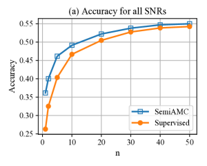
In this part, we studied the performance of SemiAMC given a large amount of unlabeled data and a small amount of labeled data. For each modulation type under each SNR, we have 500 signal samples for training, 250 signal samples for validation, and 250 signal samples for testing. We assume that for each modulation type under each SNR, only signal samples have labels in the training set, and signal samples have labels in the validation set. We train the encoder with all signal samples (without labels) in the training set, then we train the classifier and fine-tune the encoder with the labeled signal samples in the training set. The model with minimum validation loss is used to predict the classification accuracy on the test set.
To study the effectiveness of the encoder learned in the self-supervised contrastive pre-training, we directly train the encoder and classifier in a supervised way with the labeled data in the training set, and then use the model with minimum validation loss to recognize the signals in the test set. We denote this approach as “Supervised”. The classification accuracy for test signals under all SNRs and SNRS larger than zero are shown in Figure 4. We can see that SemiAMC outperforms its corresponding supervised version. This confirms the effectiveness of the encoder trained with our self-supervised contrasive learning framework. We also observe that the gap between SemiAMC and the supervised version becomes larger with the decrease in labeled data. It suggests that our framework can effectively utilize unlabeled data. Naturally, the impact of unlabeled data is larger when less data are labeled. The performance gain of SemiAMC for SNRs larger than zero (Figure 4(b)) are larger than those computed across all SNRs (Figure 4(a)). It illustrates improved effectiveness of SemiAMC in dealing with higher SNR signals.
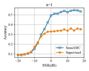
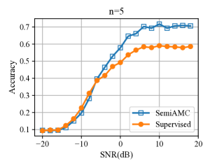
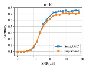
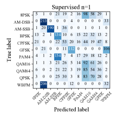
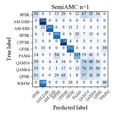
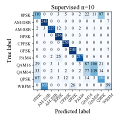
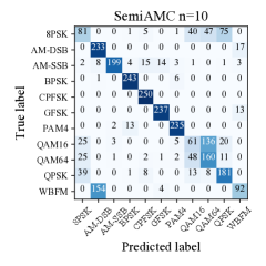
To further understand the classification accuracy under different SNR signals when different amounts of labeled data are given, we calculate the accuracy distribution under all SNR signals when n=1,5,10. The results are shown in Figure 5. We observe that the performance gain of SemiAMC compared with the supervised approach mainly comes from the signals with high SNR while SemiAMC performs similarly with the supervised approach when the SNRs are small. We also study the performance of SemiAMC of each modulation type when and the SNR is 10dB. We draw the corresponding confusion matrices in Figure 6. We observe similar accuracy patterns for different modulation types between SemiAMC and its corresponding supervised approach. For example, both of them would incorrectly recognize WBFM modulated signals as AM-DSB.
IV-E Performance under Different Amount of Unlabeled Data
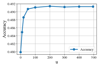
Finally, we study the recognition accuracy when different amounts of unlabeled data is given. Unlabeled data are used to train the encoder in the self-supervised pre-training part. In this experiment, we have 500 samples per SNR per modulation type for training. We assume that of the samples have labels, and use extra unlabeled samples besides the labeled samples to train SemiAMC. Figure 7 plots the overall accuracy versus the change in the amount of unlabeled data. It is observed that the classification accuracy increases with increasing amounts of unlabeled data (up to a certain level).
V Conclusion
In this paper, we proposed a novel semi-supervised deep learning framework, called SemiAMC, to accurately recognize the modulation types of radio signals. SemiAMC efficiently utilizes unlabeled data by learning representations or features through self-supervised contrastive pre-training. We conduct several experiments on a public data set to evaluate the performance of SemiAMC. The evaluation results demonstrate a non-trivial performance gain for SemiAMC compared with supervised approaches for the same amount of labeled training data, thus verifying the effectiveness of SemiAMC at utilizing unlabeled data.
VI Acknowledgements
Research reported in this paper was sponsored in part by the Army Research Laboratory under Cooperative Agreement W911NF-17-2-0196 and NSF under award CPS 20-38817, and in part by The Boeing Company. The views and conclusions contained in this document are those of the authors and should not be interpreted as representing the official policies, either expressed or implied, of the Army Research Laboratory, NSF, Boeing, or the U.S. Government. The U.S. Government is authorized to reproduce and distribute reprints for Government purposes notwithstanding any copyright notation here on.
References
- [1] C. Long, K. Chugg, and A. Polydoros, “Further results in likelihood classification of qam signals,” in Proceedings of MILCOM’94. IEEE, 1994, pp. 57–61.
- [2] N. E. Lay and A. Polydoros, “Modulation classification of signals in unknown isi environments,” in Proceedings of MILCOM’95, vol. 1. IEEE, 1995, pp. 170–174.
- [3] O. A. Dobre, A. Abdi, Y. Bar-Ness, and W. Su, “The classification of joint analog and digital modulations,” in MILCOM 2005-2005 IEEE Military Communications Conference. ieee, 2005, pp. 3010–3015.
- [4] K. Ho, W. Prokopiw, and Y. Chan, “Modulation identification of digital signals by the wavelet transform,” IEE Proceedings-Radar, Sonar and Navigation, vol. 147, no. 4, pp. 169–176, 2000.
- [5] S. Huang, Y. Yao, Z. Wei, Z. Feng, and P. Zhang, “Automatic modulation classification of overlapped sources using multiple cumulants,” IEEE Transactions on Vehicular Technology, vol. 66, no. 7, 2016.
- [6] A. Krizhevsky, I. Sutskever, and G. E. Hinton, “Imagenet classification with deep convolutional neural networks,” in Advances in neural information processing systems, 2012, pp. 1097–1105.
- [7] J. Devlin, M.-W. Chang, K. Lee, and K. Toutanova, “Bert: Pre-training of deep bidirectional transformers for language understanding,” arXiv preprint arXiv:1810.04805, 2018.
- [8] T. J. O’Shea, J. Corgan, and T. C. Clancy, “Convolutional radio modulation recognition networks,” in International conference on engineering applications of neural networks. Springer, 2016, pp. 213–226.
- [9] T. J. O’Shea, T. Roy, and T. C. Clancy, “Over-the-air deep learning based radio signal classification,” IEEE Journal of Selected Topics in Signal Processing, vol. 12, no. 1, pp. 168–179, 2018.
- [10] S. Rajendran, W. Meert, D. Giustiniano, V. Lenders, and S. Pollin, “Deep learning models for wireless signal classification with distributed low-cost spectrum sensors,” IEEE Transactions on Cognitive Communications and Networking, vol. 4, no. 3, pp. 433–445, 2018.
- [11] J. Xu, C. Luo, G. Parr, and Y. Luo, “A spatiotemporal multi-channel learning framework for automatic modulation recognition,” IEEE Wireless Communications Letters, vol. 9, no. 10, pp. 1629–1632, 2020.
- [12] L. Huang, W. Pan, Y. Zhang, L. Qian, N. Gao, and Y. Wu, “Data augmentation for deep learning-based radio modulation classification,” IEEE Access, vol. 8, pp. 1498–1506, 2019.
- [13] Q. Zheng, P. Zhao, Y. Li, H. Wang, and Y. Yang, “Spectrum interference-based two-level data augmentation method in deep learning for automatic modulation classification,” Neural Computing and Applications, pp. 1–23, 2020.
- [14] P. Wang and M. Vindiola, “Data augmentation for blind signal classification,” in MILCOM 2019-2019 IEEE Military Communications Conference (MILCOM). IEEE, 2019, pp. 305–310.
- [15] T. Chen, S. Kornblith, M. Norouzi, and G. Hinton, “A simple framework for contrastive learning of visual representations,” arXiv preprint arXiv:2002.05709, 2020.
- [16] D. Liu, T. Wang, S. Liu, R. Wang, S. Yao, and T. Abdelzaher, “Contrastive self-supervised representation learning for sensing signals from the time-frequency perspective,” in 2021 International Conference on Computer Communications and Networks (ICCCN). IEEE, 2021, pp. 1–10.
- [17] T. J. O’shea and N. West, “Radio machine learning dataset generation with gnu radio,” in Proceedings of the GNU Radio Conference, vol. 1, no. 1, 2016.
- [18] Y. Zeng, M. Zhang, F. Han, Y. Gong, and J. Zhang, “Spectrum analysis and convolutional neural network for automatic modulation recognition,” IEEE Wireless Communications Letters, vol. 8, no. 3, pp. 929–932, 2019.
- [19] E. Perenda, S. Rajendran, and S. Pollin, “Automatic modulation classification using parallel fusion of convolutional neural networks,” IEEE WIRELESS COMMUNICATIONS, 2019.
- [20] J. E. Van Engelen and H. H. Hoos, “A survey on semi-supervised learning,” Machine Learning, vol. 109, no. 2, pp. 373–440, 2020.
- [21] K. Sohn, “Improved deep metric learning with multi-class n-pair loss objective,” in Proceedings of the 30th International Conference on Neural Information Processing Systems, 2016, pp. 1857–1865.