Disentangled3D: Learning a 3D Generative Model with Disentangled Geometry and Appearance from Monocular Images
Abstract
Learning 3D generative models from a dataset of monocular images enables self-supervised 3D reasoning and controllable synthesis. State-of-the-art 3D generative models are GANs that use neural 3D volumetric representations for synthesis. Images are synthesized by rendering the volumes from a given camera. These models can disentangle the 3D scene from the camera viewpoint in any generated image. However, most models do not disentangle other factors of image formation, such as geometry and appearance. In this paper, we design a 3D GAN which can learn a disentangled model of objects, just from monocular observations. Our model can disentangle the geometry and appearance variations in the scene, i.e., we can independently sample from the geometry and appearance spaces of the generative model. This is achieved using a novel non-rigid deformable scene formulation. A 3D volume that represents an object instance is computed as a non-rigidly deformed canonical 3D volume. Our method learns the canonical volume, as well as its deformations, jointly during training. This formulation also helps us improve the disentanglement between the 3D scene and the camera viewpoints using a novel pose regularization loss defined on the 3D deformation field. In addition, we model the inverse deformations, enabling the computation of dense correspondences between images generated by our model. Finally, we design an approach to embed real images into the latent space of our model, enabling editing of real images.
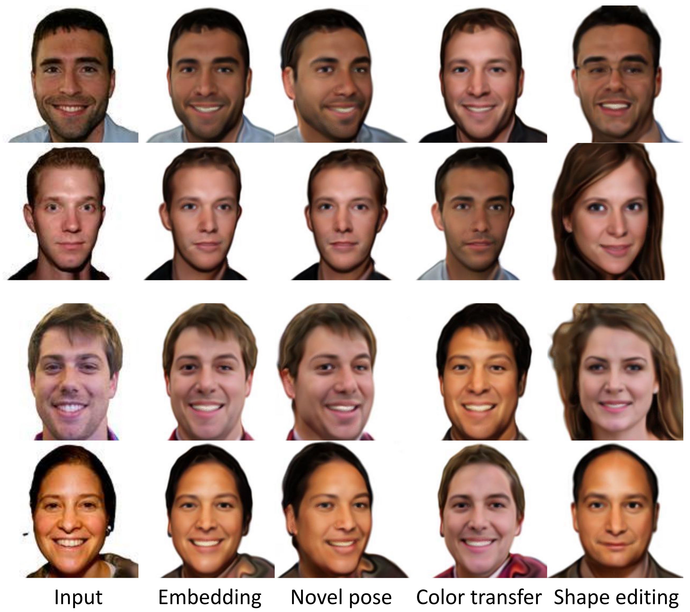
![[Uncaptioned image]](/html/2203.15926/assets/latex/Images/qualitative.jpg)
1 Introduction
State-of-the-art generative models directly operate in the image space using 2D CNNs. These models, such as StyleGAN and its variants [15, 16, 14] have achieved a high level of photorealism. However, image-based models do not offer direct control over the underlying 3D scene parameters, such as camera and geometry. While some methods add camera viewpoint control over pretrained image-based GAN models [5, 37, 17, 1], the results are limited by the quality of 3D consistency of the pretrained models.
In contrast to the image-based methods, recent approaches learn GAN models directly in the 3D space [33, 27, 2, 8, 25]. In this case, the generator network synthesizes a 3D representation of the scene as output, which can then be rendered from a virtual camera to generate the image. Since the 3D scene is explicitly modeled, the camera parameters are disentangled from the scene itself in the image synthesis process. However, other scene properties such as geometry and appearance remain entangled and cannot be controlled independently. While some 3D GAN approaches have attempted to disentangle geometry from appearance [33, 27], their design choices are not physically-motivated, which leads to inaccurate solutions where appearance information can leak through the geometry component. In contrast, our proposed approach is inspired by recent non-rigid formulations for novel viewpoint synthesis of dynamic scenes [39, 29]. These methods model the deformations in a scene observed across time, by separating the 3D reconstruction of each frame into a canonical 3D reconstruction and its deformations. Yet, even though these methods can learn to synthesize novel viewpoints of a deforming scene, they are limited to modeling a single scene, and they cannot control the appearance of the scene.
In this work, we propose D3D, a GAN with two separate and independent components for geometry and appearance. We extend the non-rigid formulation to the case of modeling multiple instances of a deformable object category, such as human heads, cats, or cars. Each instance of the object class is modeled as a deformation of a canonical volume, which is shared across the object category. Our method learns the canonical volume, as well as the instance-specific geometric deformations jointly from datasets of monocular images. The canonical volume has a fixed geometry while its appearance can be changed independent of the geometric deformations. This formulation by design motivates disentanglement between the geometric deformations and appearance variations, which has been a challenging task, especially as we are limited to monocular images for training.
In addition to the disentanglement of geometry and appearance, our formulation allows for other advantages over state-of-the-art methods. Since our geometric deformations are explicit Euclidean transformations, we can enforce useful properties in the model, such as pose consistency over the generated 3D volumes. Existing 3D GANs do not always manage to disentangle the camera viewpoint and the generated 3D volumes, especially when the hand-crafted prior camera distribution does not match the real distribution of the training dataset. We design a pose regularization loss, which can enforce the consistency of the object pose, improving the quality of camera and scene disentanglement. In addition, we learn an inverse deformation network, allowing us to compute dense correspondences between images generated by our model. Finally, we allow editing of input photographs using D3D by mapping a given image to the corresponding geometry and appearance latent codes, as well as the camera pose. In summary, this paper presents the following contributions:
-
1.
A generative model which can disentangle geometry, appearance, and camera pose in the generated images. This is enabled by a generalization of the non-rigid scene formulation to deformable object categories.
-
2.
A novel training framework for 3D GANs, which enables pose consistency of the generated volumes, as well as the computation of dense correspondences between generated images.
-
3.
Editing of real images by computing their embedding in our GAN space. This enables intuitive control over the camera pose, appearance and geometry in images.
2 Related Work
2.1 3D Generative Adversarial Networks
2D Generative adversarial networks (GANs) [7] have achieved great success in synthesizing high-fidelity images, but lack explicit control over scene parameters, and do not guarantee 3D consistency. Several attempts have been made to incorporate GANs with 3D representations for 3D-aware image synthesis. Some works directly train on 3D data [40, 3], while others only use 2D images by leveraging differentiable 3D-2D projection [25, 26, 20, 27, 11, 36, 33, 2, 9]. In this work, we focus on the latter paradigm, which is more practical, as collecting 3D scans is resource-intensive. Many methods [25, 26, 20, 27, 9] synthesize 3D features which are converted into the final images using image-based networks. This limits the quality of 3D consistency in the rendered results. Henzler et al. [11] and Szabo et al. [36] learn to generate explicit 3D voxels and meshes respectively, but produce shapes and images with limited quality. Recently, there has been a surge of interest in adopting coordinate-based neural volumetric representations [24], defined using MLPs, as the 3D representation for GANs [33, 2, 28, 44]. These approaches have achieved high-quality 3D-aware image synthesis with high-quality 3D consistency. However, the disentanglement between geometry and appearance has not been fully explored.
2.2 Disentanglement
Monocular Approaches:
Zhu et al. [47] proposed a GAN that can disentangle the shape, appearance, and camera variations in images. The final appearance is synthesized using a 2D network, which can limit the 3D consistency in the synthesized images. The closest approach to our work is GRAF [33]. The network consists of a shared backbone MLP, with separate color and density heads. The appearance latent code is provided as an input to the color head, while the shape latent code is provided as an input to the backbone. The backbone MLP corresponds to the deformation network in our design. However, unlike our deformation network, GRAF does not explicitly model 3D deformations, and the output of the backbone network lives in a higher-dimensional space. This leads to lower-quality disentanglement, where the color information can leak into the backbone network, and the appearance code can be ignored. Unlike GRAF, our framework also enables the computation of dense correspondences, which is made possible by our explicit modeling of the forward and inverse deformation fields. GIRAFFE [27] uses the same disentanglement strategy as GRAF, however, it also relies on a 2D rendering network which limits 3D consistency.
Multi-View:
Other approaches disentangle these factors using multi-view imagery. Multi-view images provide more information about the 3D geometry which makes this task easier. Xiang et al. [43] proposed NeuTex, which can disentangle the shape from appearance by learning the appearance information on a texture map. The mapping between the 3D scene coordinates and 2D texture coordinates is also learned by the method. However, NeuTex is scene-specific and is thus not a generative model, i.e., we cannot randomly sample realistic scenes from their model. Liu et al. [22] proposed a method for editing radiance fields. Their network is trained on a class of objects and enables controllable editing at test time. CodeNeRF [13] also achieves independent control over the shape and appearance components. Both these approaches share a similar design choice with GRAF, i.e., their canonical shape space does not receive a 3D input. Instead, it lives in a higher-dimensional space, which is not interpretable. Our method, in contrast, is physically inspired, as it models explicit 3D deformations between different object instances. In addition, our method is the only one that enables dense correspondences between synthesized images.
2.3 Non-Rigid NeRFs
Another category of papers [42, 31, 29, 39, 19] addresses the problem of time-varying novel-view synthesis given monocular videos. Xian et al. [42] extend the NeRF formulation to parameterize the network with time to model time-dependent view interpolation. D-NeRF [31], NR-NeRF [39], and Nerfies [29] learn a canonical representation of the entire scene from which the other frames can be obtained by learning deformations to the canonical space. These methods also propose a number of regularizers to control the deformation space. Li et al. [19] takes a different approach by learning a 3D flow field between neighbouring time samples. They supervise their method with 2D optical flow and depth predictors. In contrast to these approaches, our method is a generative model and is not limited to a given scene. In addition, we can also disentangle appearance from geometry.
3 Method

We use a neural volumetric representation to represent objects, i.e., an MLP network encodes the 3D coordinates and regresses the density and radiance values of the 3D volume [24]. The output volume can be rendered from a virtual camera using volumetric integration to produce the final image. The network is trained in an adversarial manner using monocular images as the training data.
3.1 Network Architecture
The pipeline of our method is shown in Fig. 2, which includes a generator and a discriminator. Since we want to disentangle the geometry and appearance in the scene, we model these components as individual MLP networks, represented as functions and . In addition, we use another MLP network, represented as function , to model the canonical object shape. For any object class, a shared canonical volume defined by will represent a canonical geometry. will model the deformation of a specific object instance with respect to the canonical geometry, and will represent the color of the canonical volume. Furthermore, we can optionally train an inverse deformation network that models the inverse mapping of , enabling dense correspondence (introduced in Sec. 3.4). Next, we introduce these components in detail.
Our method models color and volume density in the 3D space. For a point with coordinate , we first send it to the deformation network to obtain its corresponding point in the canonical space as
| (1) |
where is the geometry latent vector sampled from a Gaussian distribution. Thus, represents different object shapes by varying the deformation field. We can compute the volume density in the canonical space as:
| (2) |
where the canonical network does not receive any conditioning other than the input coordinate.
Next, we represent the view-dependent color, i.e., radiance, of the scene in the canonical space as:
| (3) |
Here, , is the viewing direction, and is a randomly sampled dimensional vector. Thus, we can vary the color without changing geometry by simply sampling different color latent vectors .
Disentanglement
The explicit modeling of deformation fields in our model by design encourages the disentanglement between the geometry and appearance components. Specifically, our geometry deformation network generates 3-dimensional Euclidean transformations, which is added to the input coordinate to obtain the deformed coordinate in the canonical space. This is in contrast with the state-of-the-art methods [33, 27], which use a similar network architecture, but their backbone network directly produces a high-dimensional output without any physical interpretation. This design choice hinders good disentanglement, as this high-dimensional space can also encode information about the color of the object. In contrast, our formulation strictly restricts the output of the geometry network to a 3-dimensional vector that models a coordinate offset. This makes it less likely for our method to leak color information compared to previous methods.
While our formulation discourages the color information from leaking into the geometry channel, this approach does not completely resolve all geometry-appearance ambiguities. Consider the domain of human heads where the distinct states of mouth open and mouth closed can be represented in two ways: one where the geometry component is responsible for this deformation, another, where the geometry stays the same, and the color component changes instead. While only the first solution is physically correct, both geometry and appearance changes can plausibly lead to realistic images. Note that we do not have 3D information to judge the physically correct 3D solution—we only rely on monocular images. This ambiguity cannot be resolved solely by the separation of geometry and appearance channels into separate networks. Thus, we additionally control the level of disentanglement by using different sizes of networks for the geometry and appearance components. Specifically, when the appearance network is too large, face expression changes like mouth open would tend to be represented by the appearance network as it is easier to optimize. Balancing the depths of the deformation and appearance networks ensures good disentanglement for all datasets.
3.2 Volumetric Integration
We use the volumetric neural rendering formulation, following NeRF [24]. Unlike NeRF that has multiple views of the same scene and their corresponding poses, we only have unposed monocular images. Thus, during training, a virtual camera pose is first sampled from a prior distribution. To render an image under a given camera pose, each pixel color is computed via volume integration along its corresponding camera ray with near and far bounds and as below:
| where | (4) |
Here the dependence of and on and is omitted for clarity. In practice, we implement a discretized numerical integration using stratified and hierarchical sampling, following NeRF [24]. For each sampled discrete point along the ray, we obtain and by querying our generator according to Eq.(2) and Eq.(3). With this volumetric rendering, we can render an image under any camera pose using our model. We summarize this process as , where the generator includes the , , and components mentioned earlier, and denotes the learnable parameters. This rendering process is differentiable and thus can be trained using backpropagation.
3.3 Loss Functions
Adversarial Loss
We train our generator along with a discriminator with parameters using an adversarial loss. We use the discriminator architecture from -GAN [2]. During training, the geometry latent vector , color latent vector , and camera pose are randomly sampled from their corresponding prior distributions to generate fake images, while real images are sampled from the training dataset of distribution . Our model is trained with a non-saturating GAN loss [23] as:
| (5) |
where , and is the coefficient for regularization. In practice, , , , and are randomly sampled as mini-batches, which is an approximation of taking expectation over these variables.
Pose Regularization
With the adversarial loss, the generator learns to synthesize realistic images, when rendered from camera poses sampled from the manually specified prior camera distribution. Ideally, the network learns to disentangle the pose and the 3D scene in the generated images, i.e., the generated volumes are in a consistent pose. However, in many cases, the network converges to a solution where the generated volumes have the objects in different poses. This is usually the case when the prior distribution over camera poses is inaccurate.
In our formulation, the explicit modeling of the deformation field makes it possible to enforce pose consistency of the generated volumes. To achieve this, we first compute the global rotation component of the deformation field using SVD orthogonalization [18]. Here we only consider sampled points with a rendering weight (the scalar factor applied to the color of a 3D point during integration) greater than a specified threshold. Our pose regularization loss term is then computed as
| (6) |
where is the identity matrix. We use a differentiable SVD implementation which allows training using backpropagation. This term is very different from the regularization terms introduced in existing non-rigid formulations [39, 29], where local deformations are encouraged to be rotations. This is not suitable in our case, as we are modeling deformations across object instances, which can include stretching, compression, and discontinuities. Our loss term, on the other hand, encourages the deformations to not include any global rotation, which gives rise to a disentangled solution where the camera pose variation accounts for all pose changes in the rendered images.
We first train our networks with a combination of the two loss functions
| (7) |
Then, we further model the inverse deformation field.
3.4 Inverse Deformation
Our network allows us to compute dense correspondences between rendered images. We enable this by training an inverse deformation network with parameters . Since we are using a volumetric representation, multiple points in the volume are responsible for the color at any pixel. Dense correspondences, where a pixel in an image has a correspondence with only one pixel in another image, is not trivial to define. Thus, we simplify the formulation for the training of the inverse network by limiting its domain to points around the expected surface of the volume, which can be obtained by taking the expectation of depth using the volume rendering weights. For any such point , we can compute the canonical coordinate via Eq. 1 and use the inverse network to go back to the deformed space as . We can formulate the following constraint on the inverse deformation network:
| (8) |
Here, is a rendered image of the volume at the resolution being used for training. are sampled from the image using the expected depth value. is an operation that computes the color at the pixel which projects to, using bilinear interpolation. The first term in Eq. 8 penalizes 3D geometric deviations, while the second term can also use color information to refine the correspondences. After pretraining our networks with the loss as defined in Eq. 7, we first train the inverse network using , and finally jointly train all components in our architecture with the following loss:
| (9) |
This joint optimization of both forward and inverse deformation networks further improves dense correspondences. Note that we do not include the inverse loss from the beginning as it can bias the deformation network to generate very small deformations, making disentanglement challenging.

3.5 Embedding
Given our trained model and a real image, we could diretly optimize for the latent vector and camera pose in an iterative manner [2, 41]. However, this strategy is inefficient, and can lead to lower-quality results. We therefore learn an encoder that takes an image as input and regresses the latent vectors and camera pose. We make use of a pre-trained ResNet [10] as our encoder backbone. The encoder is trained on monocular images (FFHQ [15]), using our trained GAN as the decoder, in a self supervised manner, using the following loss function:
| (10) |
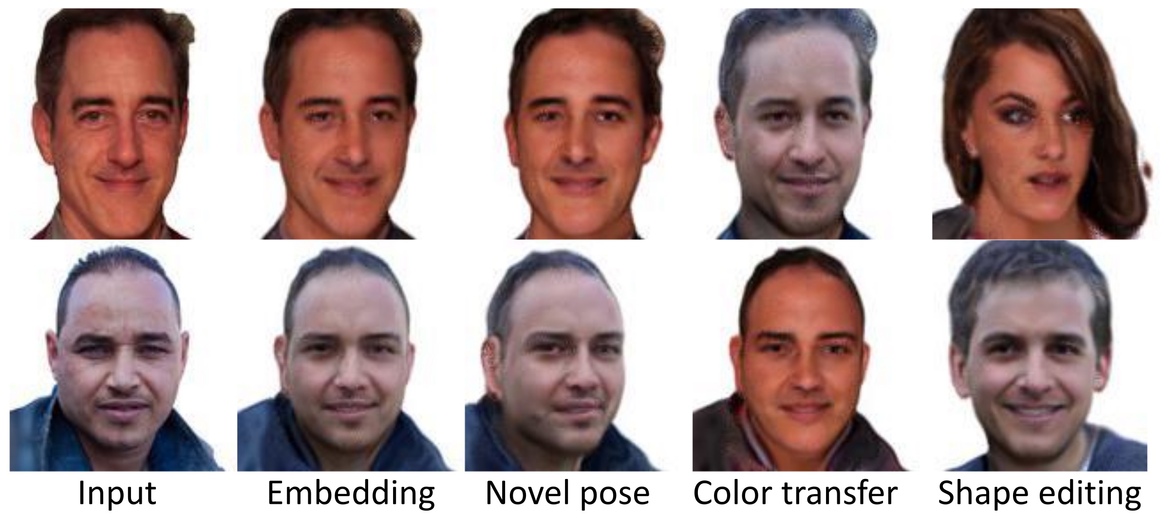
where, denotes the learnable parameters of the encoder. is an reconstruction term, and is a perceptual term defined using the features of the VGG network. encourages the predicted latent vectors to stay close to the average values. The encoded results are robust, but can still miss fine-scale details. We first refine the results of the encoder using iterative optimization, and finally fine-tune the generator network for the given image. We show that this strategy leads to high-quality results without degrading the disentanglement properties (see Fig. 7) of the generator. Please refer to the supplemental for more details.
4 Results
Datasets
We demonstrate the results of our method D3D on four datasets: FFHQ [15], VoxCeleb2 [4], Cats [46], and CARLA [6, 33]. FFHQ and VoxCeleb2 are datasets of head portraits. FFHQ includes a diverse set of static images, while VoxCeleb2 is a large-scale video dataset with larger viewpoint and expression variations. We randomly sample a few frames from each video for VoxCeleb2. Cats is a dataset of cat faces, and CARLA is a dataset of synthetic cars with large viewpoint variations. While cars are not deformable, different car instances can be considered as deformations of a shared template. The instances of these datasets share a similar geometry with varying deformations, thus, they are suitable for our task. Since we are only interested in modeling objects, we remove the backgrounds in portrait images [45]. However, because cat images have very little background, we do not segment them.
Training Details
We use the same network architecture for all datasets. Training is done in a coarse-to-fine fashion, similar to -GAN [2]. We use the same camera pose distribution as used in -GAN. We train at resolution on FFHQ, VoxCeleb2, and Cats, and resolution on CARLA. All quantitative evaluations are performed at resolution (once trained, images can be rendered at any resolution due to the neural scene representation). Please refer to the supplemental material for the hyperparameters.
Qualitative Results
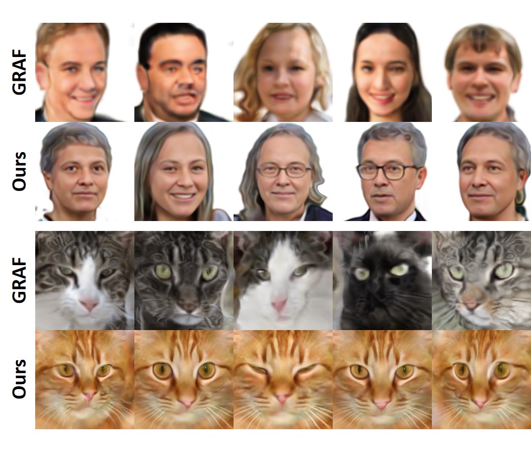
We first present qualitative results of our method on all four datasets in Fig. 1 and Fig. 3. Our method is capable of synthesizing objects in multiple poses due to the 3D nature of the generator. We can disentangle the geometry and appearance variations well for all object classes. This is true even under challenging deformations, such as deformations due to hairstyle and mouth expressions. We compare the quality of disentanglement with GRAF [33] in Fig. 4. Our method significantly outperforms GRAF in terms of disentanglement. As explained in Sec. 3.1, GRAF also encodes appearance information in the geometry code due to the high-dimensional output of its backbone. In contrast, our explicit deformation enables higher-quality disentanglement.

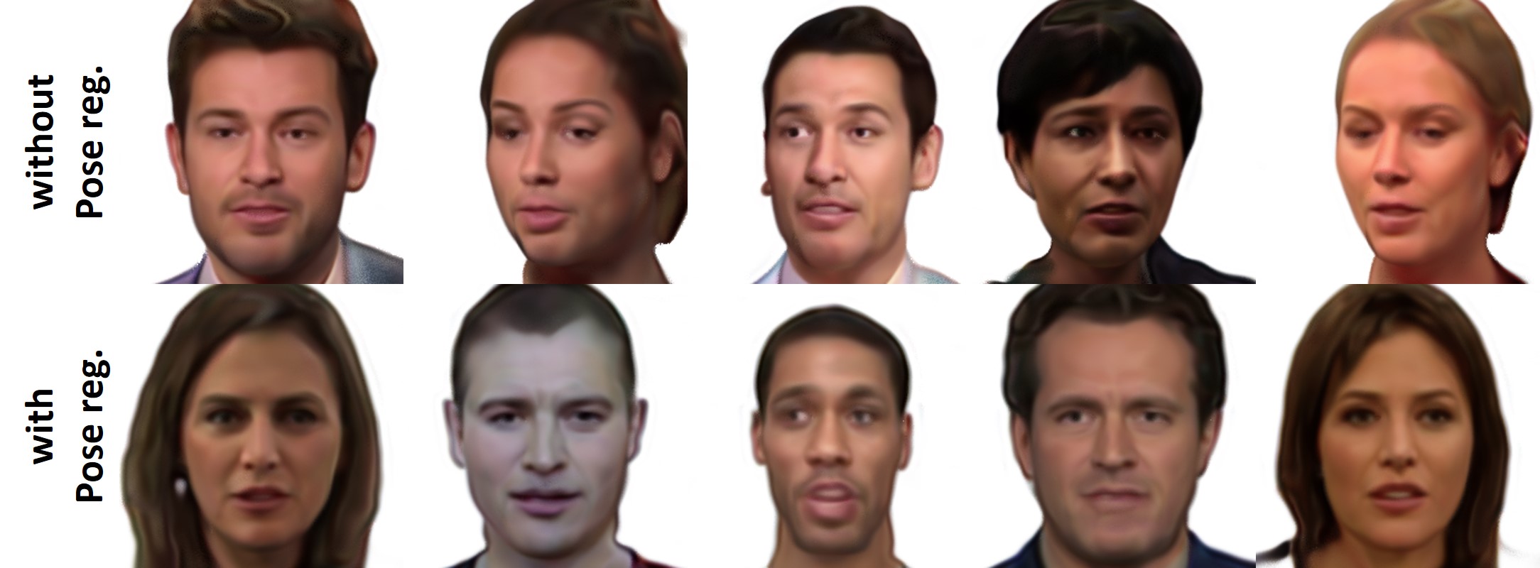
We evaluate the inverse deformation network by visualizing the dense correspondences in Fig. 5. We first provide image-level annotations on one image generated by D3D. These annotations can then be transferred to any other sample of the model using the dense correspondences. Our model learns correspondences without any explicit supervision, even for objects with large deformations. This enables applications such as one-shot segmentation transfer and keypoint annotation. In Fig. 6, we further visualize the effectiveness of the proposed pose regularization loss. Without this loss, the geometry component tends to entangle the geometry with camera viewpoint. This is most evident when training with VoxCeleb2 [4] dataset. While this dataset has larger pose varrations compared to FFHQ [15], we used the same prior pose distribution, which could lead to the geometry network also compensating for the inaccurate distribution. Our loss term disambiguates pose and the 3D scene, reducing the burden of estimating a very accurate pose distribution.
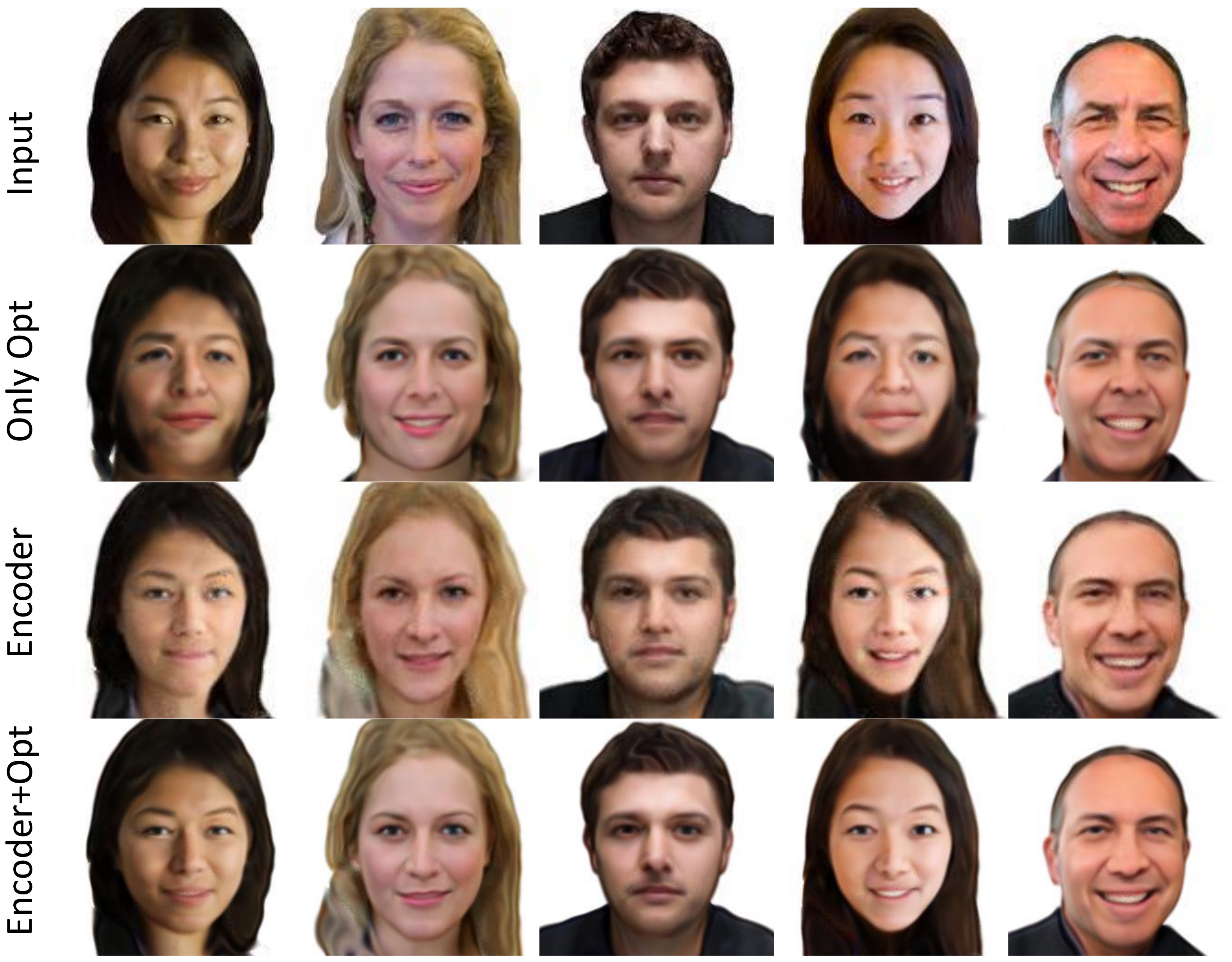
We also show embeddings of real images [34] in Fig. 7. Using our inversion method, we can achieve high-quality embeddings which enables several applications such as pose editing, shape editing, and appearance editing. For example, we can transfer the appearance of one portrait image to another, without changing the geometry. We recommend readers refer to the supplementary material for more results.
Quantitative Results
| FFHQ | VoxCeleb2 | Cats | Carla | |
|---|---|---|---|---|
| GRAF [33] | 43.32 | 35.28 | 22.64 | 37.53 |
| Ours | 28.18 | 16.51 | 16.96 | 31.13 |
|
|
|
|
|||||||||
|---|---|---|---|---|---|---|---|---|---|---|---|---|
| FFHQ | 13.22 | 13.98 | 19.99 | 28.18 |
|
|
|
|||||||
|---|---|---|---|---|---|---|---|---|---|
| -GAN | 0.15 | 0.96 | 0.15 | ||||||
| GRAF | 0.17 | 0.08 | 0.04 | ||||||
| Ours
(256-dim) |
0.13 | 0.11 | 0.07 | ||||||
| Ours
(No inverse) |
0.06 | 0.40 | 0.15 | ||||||
| Ours
(Complete) |
0.05 | 0.39 | 0.16 |
We first provide the commonly reported FID scores [12] for images generated by our model, as well as those for GRAF [33] in Table 11. The FID scores are computed using image samples. Our approach outperforms GRAF on all datasets. We also perform an ablation study on FFHQ with several baselines in Table 2. “Ours (256-dim)” is a baseline that implements the design of GRAF in our training framework, i.e., directly provides a 256-dimensional vector as output, which is sent to and . Other network architecture and training details are equivalent to our method. However, this design makes it infeasible to use the pose consistency loss and inverse deformations, so we disable them. This framework achieves a lower FID compared to our complete model, however, it does not achieve high-quality disentanglement due to the same reasons as for GRAF, see the supplemental document. “Ours (No inverse)” is our method without the inverse deformations. This architecture constraints the network by limiting to output a 3-dimensional deformation of coordinates. This leads to good disentanglement at the cost of slightly higher FID. “Ours (Complete)” further incorporates the inverse deformation network, which allows us to compute dense correspondences. While this enables broader interesting applications, it again comes at a cost of higher FID scores due to stronger regularization of the deformation field. We also report the FID score of -GAN [2], which is comparable to our 256-dimensional baseline. Note that -GAN does not enable any disentanglement between the geometry and appearance components.
We quantitatively evaluate the quality of disentanglement in Table 3. We describe two novel metrics to evaluate this. To evaluate the consistency of appearance with changing geometry, we measure the standard deviation of the average color in a semantically well-defined region, which could be obtained via an off-the-shelf segmentation model [45]. We use the hair region for human heads to compute this metric for networks trained on FFHQ [15]. We sample images from the GAN with a fixed appearance code and varying geometry codes. The standard deviation of the average hair color can be used as a metric, as a lower value would imply consistent appearance across different shapes. We compute this standard deviation for appearance codes and report the average over the values. Our approach significantly outperforms GRAF [33] and -GAN [2]. Since -GAN does not have different appearance and geometry codes, we simply sample images from their model and use the numbers as a baseline.
To evaluate the geometry consistency for a fixed geometry code with varying appearances, we use sparse facial keypoints for evaluation. We measure the standard deviation of facial landmarks computed using an off-the-shelf tool [32] across samples with a shared geometry code and different randomly sampled appearance codes. We render all images in the same pose, in order to eliminate additional factors of variance. This evaluation is repeated for different geometry codes and the error is averaged over these geometry codes, and over the landmarks. A lower number with the geometry consistency metric implies that varying the appearance code is less likely to cause geometry change in the image. While we outperform the -GAN baseline, GRAF [33] achieves a better score. This is due to the fact that the appearance variations are limited for GRAF, as the appearance information also leaks into the geometry component. We further evaluate this using an appearance variation metric for these images. This metric is defined exactly the same as the appearance consistency metric. Specifically, for the set of images, we calculate the standard deviation over the average hair color over the 100 images with different appearance codes, and average over the 10 geometry codes. As shown in Table 3, our method achieves the highest value, implying that our appearance component better captures the appearance variations of the dataset. We also evaluate both baselines using these metrics. As expected, the “256-dim“ baseline performs similar to GRAF, while the numbers are similar without the inverse network
5 Conclusion & Discussion
We have presented an approach to learn disentangled 3D GANs from monocular images. In addition to disentanglement, our formulation enables the computation of dense correspondences, enabling exciting applications. Although we have demonstrated compelling results, our method has several limitations. Like other 3D GANs, our results do not reach the photorealism quality and image resolutions of 2D GANs. The disentanglement and correspondences come at the cost of a drop in image quality (see Table 2). In addition, we use an off-the-shelf background segmentation tool which limits us from being completely unsupervised. Nevertheless, our approach achieves high image quality and disentanglement, significantly outperforming the state of the art. We hope that it inspires further work on self-supervised learning of 3D generative models.
References
- [1] Mallikarjun BR, Ayush Tewari, Abdallah Dib, Tim Weyrich, Bernd Bickel, Hans-Peter Seidel, Hanspeter Pfister, Wojciech Matusik, Louis Chevallier, Mohamed Elgharib, et al. Photoapp: Photorealistic appearance editing of head portraits. ACM Transactions on Graphics, 40(4):1–16, 2021.
- [2] Eric Chan, Marco Monteiro, Petr Kellnhofer, Jiajun Wu, and Gordon Wetzstein. pi-gan: Periodic implicit generative adversarial networks for 3d-aware image synthesis. In arXiv, 2020.
- [3] Zhiqin Chen, Vladimir G Kim, Matthew Fisher, Noam Aigerman, Hao Zhang, and Siddhartha Chaudhuri. Decor-gan: 3d shape detailization by conditional refinement. In Proceedings of the IEEE/CVF Conference on Computer Vision and Pattern Recognition, pages 15740–15749, 2021.
- [4] J. S. Chung, A. Nagrani, and A. Zisserman. Voxceleb2: Deep speaker recognition. In INTERSPEECH, 2018.
- [5] Yu Deng, Jiaolong Yang, Dong Chen, Fang Wen, and Xin Tong. Disentangled and controllable face image generation via 3d imitative-contrastive learning. In Proceedings of the IEEE/CVF Conference on Computer Vision and Pattern Recognition, pages 5154–5163, 2020.
- [6] Alexey Dosovitskiy, German Ros, Felipe Codevilla, Antonio Lopez, and Vladlen Koltun. Carla: An open urban driving simulator. In Conference on robot learning, pages 1–16. PMLR, 2017.
- [7] Ian Goodfellow, Jean Pouget-Abadie, Mehdi Mirza, Bing Xu, David Warde-Farley, Sherjil Ozair, Aaron Courville, and Yoshua Bengio. Generative adversarial nets. In NIPS, 2014.
- [8] Jiatao Gu, Lingjie Liu, Peng Wang, and Christian Theobalt. Stylenerf: A style-based 3d-aware generator for high-resolution image synthesis, 2021.
- [9] Zekun Hao, Arun Mallya, Serge Belongie, and Ming-Yu Liu. GANcraft: Unsupervised 3D Neural Rendering of Minecraft Worlds. In ICCV, 2021.
- [10] Kaiming He, Xiangyu Zhang, Shaoqing Ren, and Jian Sun. Deep residual learning for image recognition. In 2016 IEEE Conference on Computer Vision and Pattern Recognition, CVPR 2016, Las Vegas, NV, USA, June 27-30, 2016, pages 770–778. IEEE Computer Society, 2016.
- [11] Philipp Henzler, Niloy J Mitra, and Tobias Ritschel. Escaping plato’s cave: 3d shape from adversarial rendering. In ICCV, 2019.
- [12] Martin Heusel, Hubert Ramsauer, Thomas Unterthiner, Bernhard Nessler, and Sepp Hochreiter. Gans trained by a two time-scale update rule converge to a local nash equilibrium. Advances in neural information processing systems, 30, 2017.
- [13] Wonbong Jang and Lourdes Agapito. Codenerf: Disentangled neural radiance fields for object categories. arXiv preprint arXiv:2109.01750, 2021.
- [14] Tero Karras, Miika Aittala, Samuli Laine, Erik Härkönen, Janne Hellsten, Jaakko Lehtinen, and Timo Aila. Alias-free generative adversarial networks. In Proc. NeurIPS, 2021.
- [15] Tero Karras, Samuli Laine, and Timo Aila. A style-based generator architecture for generative adversarial networks. In Proceedings of the IEEE/CVF Conference on Computer Vision and Pattern Recognition (CVPR), June 2019.
- [16] Tero Karras, Samuli Laine, Miika Aittala, Janne Hellsten, Jaakko Lehtinen, and Timo Aila. Analyzing and improving the image quality of stylegan. In Proceedings of the IEEE/CVF Conference on Computer Vision and Pattern Recognition, pages 8110–8119, 2020.
- [17] Thomas Leimkühler and George Drettakis. Freestylegan: Free-view editable portrait rendering with the camera manifold. 40(6), 2021.
- [18] Jake Levinson, Carlos Esteves, Kefan Chen, Noah Snavely, Angjoo Kanazawa, Afshin Rostamizadeh, and Ameesh Makadia. An analysis of svd for deep rotation estimation. arXiv preprint arXiv:2006.14616, 2020.
- [19] Zhengqi Li, Simon Niklaus, Noah Snavely, and Oliver Wang. Neural scene flow fields for space-time view synthesis of dynamic scenes. In Proceedings of the IEEE/CVF Conference on Computer Vision and Pattern Recognition, pages 6498–6508, 2021.
- [20] Yiyi Liao, Katja Schwarz, Lars Mescheder, and Andreas Geiger. Towards unsupervised learning of generative models for 3d controllable image synthesis. In CVPR, 2020.
- [21] Rosanne Liu, Joel Lehman, Piero Molino, Felipe Petroski Such, Eric Frank, Alex Sergeev, and Jason Yosinski. An intriguing failing of convolutional neural networks and the coordconv solution. In NeurIPS, 2018.
- [22] Steven Liu, Xiuming Zhang, Zhoutong Zhang, Richard Zhang, Jun-Yan Zhu, and Bryan Russell. Editing conditional radiance fields, 2021.
- [23] Lars Mescheder, Andreas Geiger, and Sebastian Nowozin. Which training methods for gans do actually converge? In ICML, 2018.
- [24] Ben Mildenhall, Pratul P Srinivasan, Matthew Tancik, Jonathan T Barron, Ravi Ramamoorthi, and Ren Ng. Nerf: Representing scenes as neural radiance fields for view synthesis. In ECCV, 2020.
- [25] Thu Nguyen-Phuoc, Chuan Li, Lucas Theis, Christian Richardt, and Yong-Liang Yang. Hologan: Unsupervised learning of 3d representations from natural images. In Proceedings of the IEEE/CVF International Conference on Computer Vision, pages 7588–7597, 2019.
- [26] Thu Nguyen-Phuoc, Christian Richardt, Long Mai, Yong-Liang Yang, and Niloy Mitra. Blockgan: Learning 3d object-aware scene representations from unlabelled images. arXiv preprint arXiv:2002.08988, 2020.
- [27] Michael Niemeyer and Andreas Geiger. Giraffe: Representing scenes as compositional generative neural feature fields. In Proceedings of the IEEE/CVF Conference on Computer Vision and Pattern Recognition, pages 11453–11464, 2021.
- [28] Xingang Pan, Xudong Xu, Chen Change Loy, Christian Theobalt, and Bo Dai. A shading-guided generative implicit model for shape-accurate 3d-aware image synthesis. In Advances in Neural Information Processing Systems (NeurIPS), 2021.
- [29] Keunhong Park, Utkarsh Sinha, Jonathan T. Barron, Sofien Bouaziz, Dan B Goldman, Steven M. Seitz, and Ricardo Martin-Brualla. Nerfies: Deformable neural radiance fields. ICCV, 2021.
- [30] Ethan Perez, Florian Strub, Harm De Vries, Vincent Dumoulin, and Aaron Courville. Film: Visual reasoning with a general conditioning layer. In AAAI, 2018.
- [31] Albert Pumarola, Enric Corona, Gerard Pons-Moll, and Francesc Moreno-Noguer. D-NeRF: Neural Radiance Fields for Dynamic Scenes. In Proceedings of the IEEE/CVF Conference on Computer Vision and Pattern Recognition, 2020.
- [32] Jason M Saragih, Simon Lucey, and Jeffrey F Cohn. Deformable model fitting by regularized landmark mean-shift. International journal of computer vision, 91(2):200–215, 2011.
- [33] Katja Schwarz, Yiyi Liao, Michael Niemeyer, and Andreas Geiger. Graf: Generative radiance fields for 3d-aware image synthesis. In Advances in Neural Information Processing Systems (NeurIPS), 2020.
- [34] YiChang Shih, Sylvain Paris, Connelly Barnes, William T. Freeman, and Frédo Durand. Style transfer for headshot portraits. ACM Trans. on Graph. (Proceedings of SIGGRAPH), 33(4), 2014.
- [35] Vincent Sitzmann, Julien N.P. Martel, Alexander W. Bergman, David B. Lindell, and Gordon Wetzstein. Implicit neural representations with periodic activation functions. In Proc. NeurIPS, 2020.
- [36] Attila Szabó, Givi Meishvili, and Paolo Favaro. Unsupervised generative 3d shape learning from natural images. arXiv preprint arXiv:1910.00287, 2019.
- [37] Ayush Tewari, Mohamed Elgharib, Gaurav Bharaj, Florian Bernard, Hans-Peter Seidel, Patrick Pérez, Michael Zollhofer, and Christian Theobalt. Stylerig: Rigging stylegan for 3d control over portrait images. In Proceedings of the IEEE/CVF Conference on Computer Vision and Pattern Recognition, pages 6142–6151, 2020.
- [38] Ayush Tewari, Michael Zollhofer, Hyeongwoo Kim, Pablo Garrido, Florian Bernard, Patrick Perez, and Christian Theobalt. Mofa: Model-based deep convolutional face autoencoder for unsupervised monocular reconstruction. In Proceedings of the IEEE International Conference on Computer Vision Workshops, pages 1274–1283, 2017.
- [39] Edgar Tretschk, Ayush Tewari, Vladislav Golyanik, Michael Zollhöfer, Christoph Lassner, and Christian Theobalt. Non-rigid neural radiance fields: Reconstruction and novel view synthesis of a dynamic scene from monocular video. In IEEE International Conference on Computer Vision (ICCV). IEEE, 2021.
- [40] Jiajun Wu, Chengkai Zhang, Tianfan Xue, Bill Freeman, and Josh Tenenbaum. Learning a probabilistic latent space of object shapes via 3d generative-adversarial modeling. In NIPS, 2016.
- [41] Weihao Xia, Yulun Zhang, Yujiu Yang, Jing-Hao Xue, Bolei Zhou, and Ming-Hsuan Yang. Gan inversion: A survey. arXiv preprint arXiv:2101.05278, 2021.
- [42] Wenqi Xian, Jia-Bin Huang, Johannes Kopf, and Changil Kim. Space-time neural irradiance fields for free-viewpoint video. In Proceedings of the IEEE/CVF Conference on Computer Vision and Pattern Recognition (CVPR), pages 9421–9431, 2021.
- [43] Fanbo Xiang, Zexiang Xu, Milos Hasan, Yannick Hold-Geoffroy, Kalyan Sunkavalli, and Hao Su. Neutex: Neural texture mapping for volumetric neural rendering. In Proceedings of the IEEE/CVF Conference on Computer Vision and Pattern Recognition, pages 7119–7128, 2021.
- [44] Xudong Xu, Xingang Pan, Dahua Lin, and Bo Dai. Generative occupancy fields for 3d surface-aware image synthesis. In Advances in Neural Information Processing Systems(NeurIPS), 2021.
- [45] Changqian Yu, Jingbo Wang, Chao Peng, Changxin Gao, Gang Yu, and Nong Sang. Bisenet: Bilateral segmentation network for real-time semantic segmentation. In Proceedings of the European conference on computer vision (ECCV), pages 325–341, 2018.
- [46] Weiwei Zhang, Jian Sun, and Xiaoou Tang. Cat head detection-how to effectively exploit shape and texture features. In European Conference on Computer Vision, pages 802–816. Springer, 2008.
- [47] Jun-Yan Zhu, Zhoutong Zhang, Chengkai Zhang, Jiajun Wu, Antonio Torralba, Josh Tenenbaum, and Bill Freeman. Visual object networks: Image generation with disentangled 3d representations. In NeurIPS, 2018.
Appendix A Training Details
Network Architecture
Our generator network consists of a geometry deformation network , an appearance network , and a canonical geometry network . Both and include a mapping network and a main network following the design of -GAN [2]. The mapping networks are implemented as MLPs with LeakyReLU activations, see Table 4. The randomly sampled inputs and are used as inputs to the mapping networks. The output of the mapping networks are one-dimensional vectors of dimensions and , where and are the number of SIREN layers in the main networks of and respectively. The main networks are implemented as MLPs with SIREN layers [35] and FiLM conditioning [30], see Table 6 and Table 7. Each layer of the main network receives one -dimensional component of the output of the mapping network. The canonical network does not receive any input other than the co-ordinates in the canonical space. We follow the initialization method of [35] for , , and , where the first layer is initialized with larger values. The final layer of is initialized such that the deformations at the first iteration are all zeros. The inverse deformation network is implemented exactly as , except that it receives the input in the canonical space and models the inverse deformation. As for the discriminator, we adopt the same model architecture as in [2], which is a convolutional neural network with residual connections [10] and CoordConv layers [21].
As explained in the main paper, we control the level of disentanglement using the number of SIREN layers in and , i.e., and , respectively. We set and for FFHQ [15], VoxCeleb2 [4], and Cats [46]. For Carla [6], we set and . We will show results where changing the relative depths of these networks can lead to poor disentanglement.
| Input | Layer | Activation | Output Dim. |
|---|---|---|---|
| or | Linear | LeakyReLU (0.2) | 256 |
| - | Linear | LeakyReLU (0.2) | 256 |
| - | Linear | LeakyReLU (0.2) | 256 |
| - | Linear | None | 256 2 |
| Input | Layer | Activation | Output Dim. |
|---|---|---|---|
| Linear | Sine | 256 | |
| - | Linear | Sine | 256 |
| - | Linear | Sine | 256 |
| - | Linear | Sine | 256 |
| - | Linear | None | 1 |
| Input | Layer | Activation | Output Dim. |
|---|---|---|---|
| , Map() | Linear | FiLM+Sine | 256 |
| -, Map() | … | … | … |
| -, Map() | … | … | … |
| -, Map() | Linear | None | 3 |
| Input | Layer | Activation | Output Dim. |
|---|---|---|---|
| , Map() | Linear | FiLM+Sine | 256 |
| -, Map() | … | … | … |
| -, Map() | … | … | … |
| -, Map(), | Linear | FiLM+Sine | 256 |
| -, Map() | Linear | Sigmoid | 3 |
Hyperparameters
| Hyperparameter | Dataset | Value |
|---|---|---|
| FFHQ | 1.0 | |
| VoxCeleb2 | 1.0 | |
| Cats | 0.5 | |
| Carla | 10.0 | |
| FFHQ | 50.0 | |
| VoxCeleb2 | 50.0 | |
| Cats | 5.0 | |
| Carla | 50.0 | |
| FFHQ | 0.001 | |
| VoxCeleb2 | 0.001 | |
| Cats | 0.001 | |
| Carla | 0.001 | |
| FFHQ | 1.0 | |
| VoxCeleb2 | 1.0 | |
| Cats | 1.0 | |
| Carla | 1.0 |
| Dataset | Iteration (in k) | Batch Size | Image Size | ||
|---|---|---|---|---|---|
| FFHQ | 0-20 | 208 | 32 | 2e-5 | 2e-4 |
| 20-60 | 52 | 64 | 2e-5 | 2e-4 | |
| 60- | 52 | 64 | 1e-5 | 1e-4 | |
| VoxCeleb2 | 0-20 | 208 | 32 | 2e-5 | 2e-4 |
| 20-60 | 52 | 64 | 2e-5 | 2e-4 | |
| 60- | 52 | 64 | 1e-5 | 1e-4 | |
| Cats | 0-10 | 208 | 32 | 6e-5 | 2e-4 |
| 10- | 52 | 64 | 6e-5 | 2e-4 | |
| Carla | 0-10 | 60 | 32 | 4e-5 | 4e-4 |
| 10-26 | 20 | 64 | 2e-5 | 2e-4 | |
| 26- | 18 | 128 | 10e-6 | 10e-5 |
Embedding Architecture
Our encoder network consists of a pretrained ResNet-18 [10] as the backbone. We add two linear layers to regress the camera pose and latent vectors. Inspired by -GAN [2], we learn to directly regress the frequencies and phase shifts, i.e., the output space of the mapping networks for the geometry and appearance components. We train the encoder on FFHQ [15]. We set and and use a learning rate of .
At test time, to further improve the result, we fine-tune the regressed latent vectors using iterative optimization for iterations with a learning rate of . We finally fine-tune the generator network for another iterations with a learning rate of . We show that this strategy leads to high-quality results without degrading the disentanglement properties (see Fig. 14) of the generator.
We also show that this approach works better than optimization-only method (see Fig. 13), where we iteratively optimize for the latent vectors and camera pose using reconstruction loss. For optimization-only approach, we update the latent vectors and camera pose while keeping the GAN fixed for iterations with a learning rate of . And then finetune GAN as well for another iterations with a learning rate of . We can observe (Fig. 13, 14) that using encoder initialization helps obtain better results while still preserving the disentanglement properties of our model.
Appendix B Results
| Pose Consistency | ||
|---|---|---|
| pi-GAN | 0.34 | |
|
0.16 | |
| Ours | 0.03 |
Qualitative Results
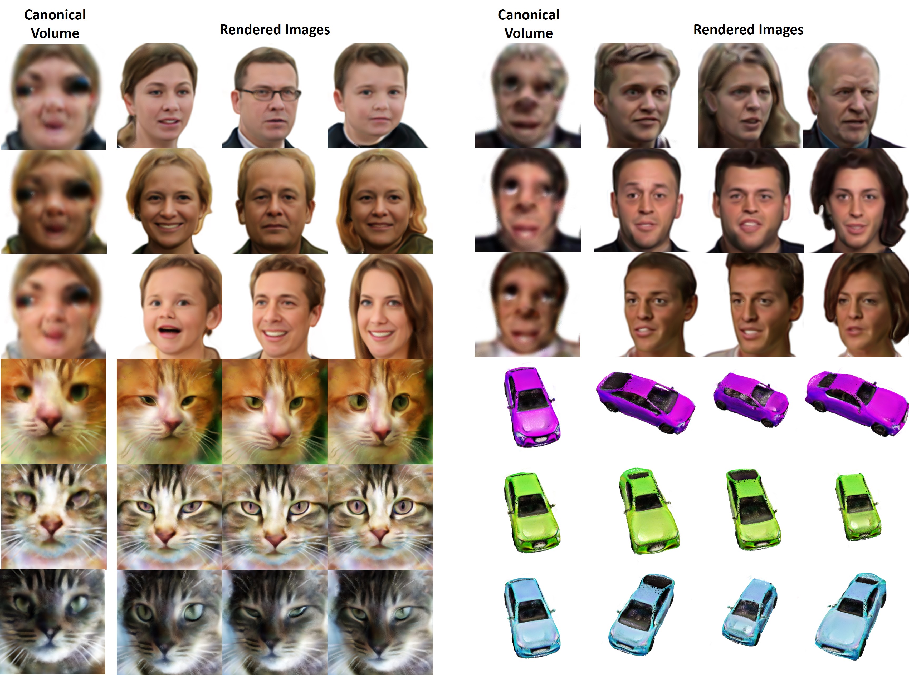
We show more results of our method along with visualizations of the learned canonical volume in Fig. 8.
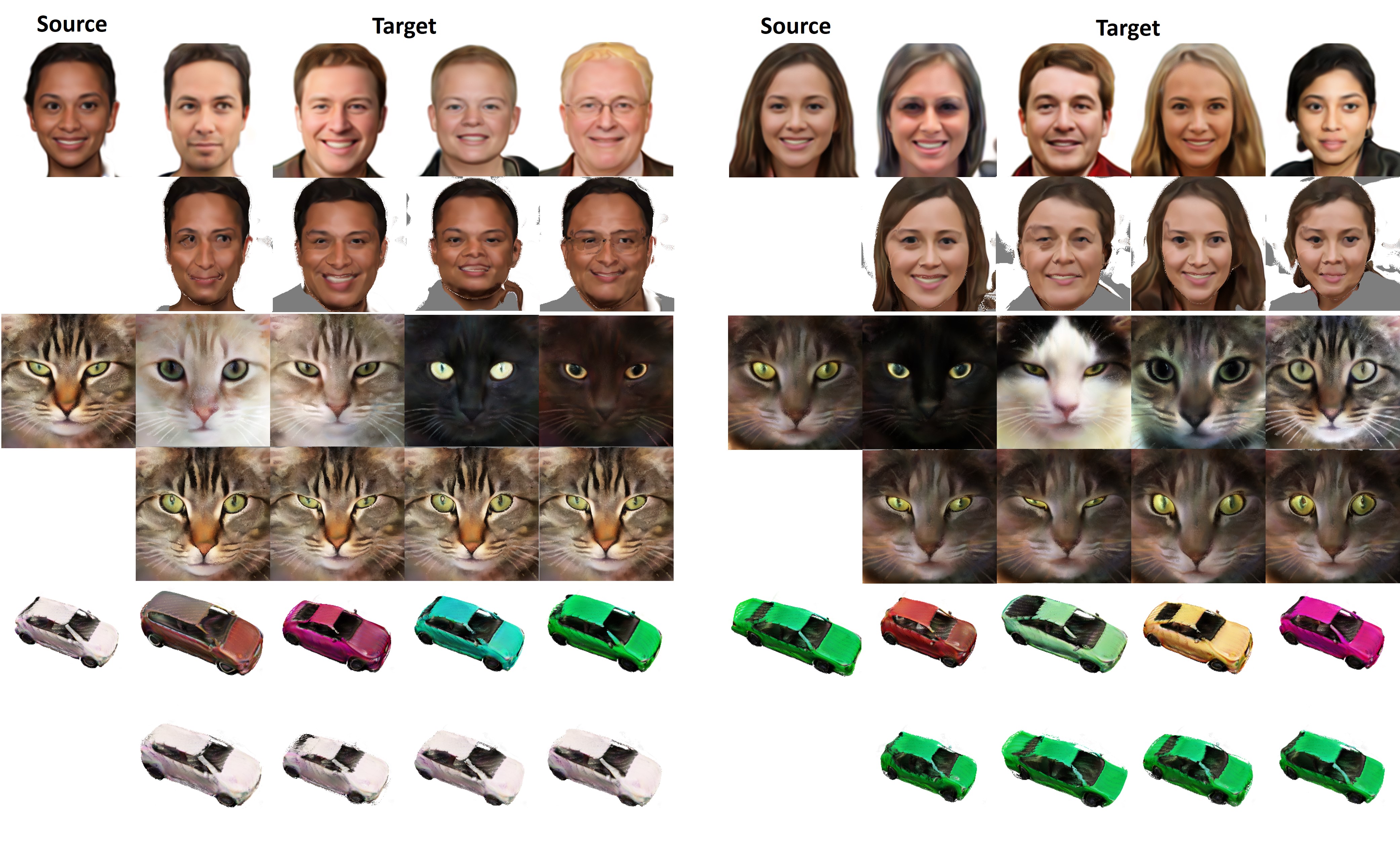
We present more visualizations of the learned correspondences in Fig. 9. The appearance of one sample is transferred to another using the correspondences. This shows the applicability of the correspondences for any task where one image annotation can be transferred to all other samples of the model.
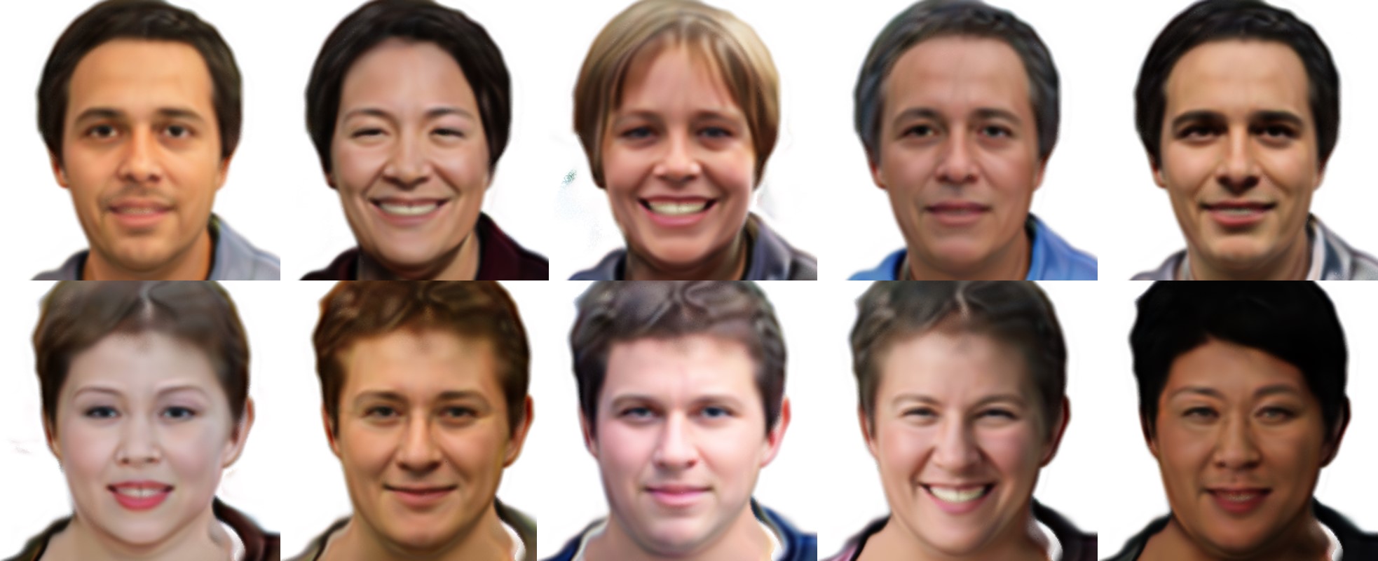
As mentioned earlier, the level of disentanglement is controlled using the relative depths of the geometry and appearance networks. We show in Fig. 10 that a large appearance network can lead to lower-quality disentanglement, where geometric features such as expressions are compensated by the appearance component. We set and for these results.

In the main paper, we presented quantitative results of a baseline where the canonical network receives a high-dimensional input like GRAF [33]. Fig. 11 shows qualitative results of this baseline. As explained in the main paper, this baseline has similar limitations as GRAF, where the geometry network also changes the appearance of the object.
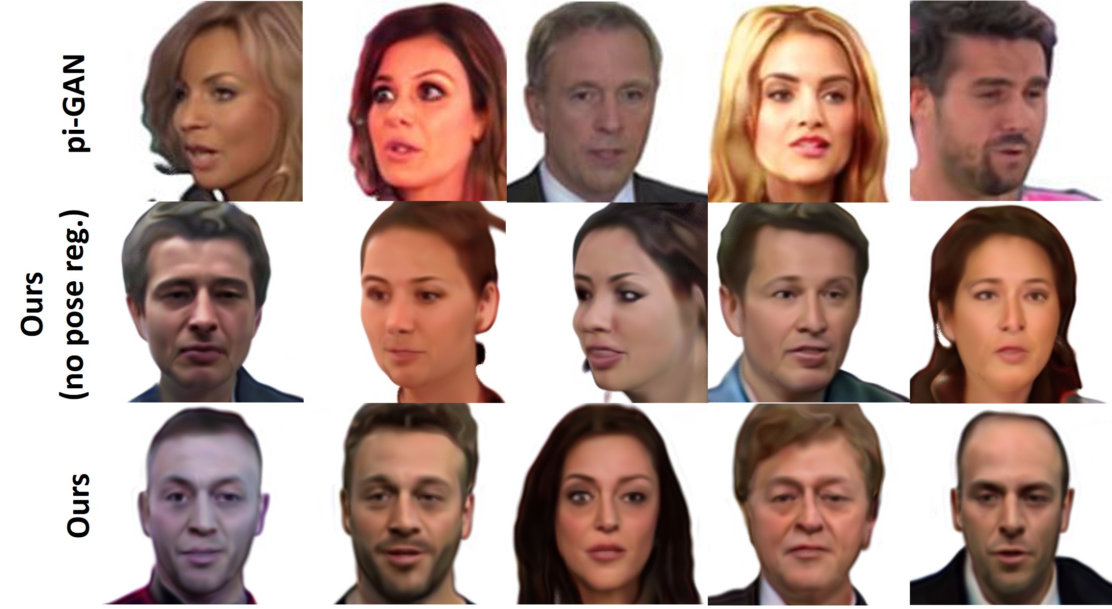
Fig. 12 shows more results for evaluation of the pose regularization. Without our proposed regularization, the model does not properly disentangle the object and the camera pose. This limitation is also shared with -GAN [2].

We further show some results of correspondence and depth visualizations on real images in Fig. 15. Unlike the encoders used in other results, we trained the encoder for this result on the generator which was trained with the inverse network.
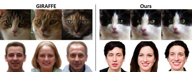
We also compare to GIRAFFE [27] in Fig. 16. Our method maintains the consistency of both pose and shape components better. Quantitatively, GIRAFFE achieves similar scores compared to our method on FFHQ using the metrics defined in the main paper. It achieves an appearance consistency score of 0.05, geometry consistency score of 0.32, and appearance variation score of 0.09. However, ours results have better multi-view consistency, and better qualitative disentanglement as shown in Fig. 16.
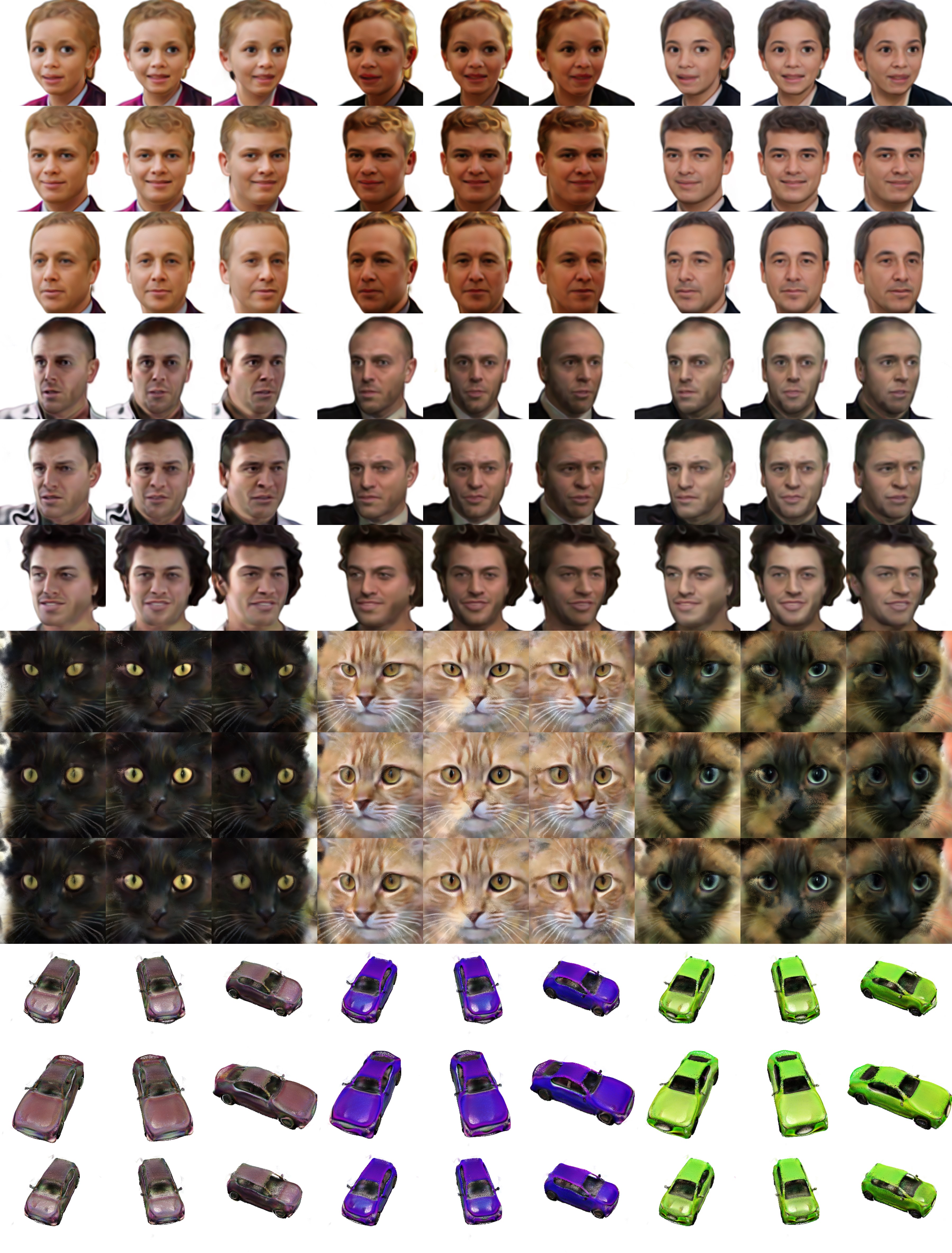
We show several more results of our GAN in Fig. 17.
Quantitative results
| FFHQ | VoxCeleb2 | Cats | |
|---|---|---|---|
| GRAF [33] | 25.36 | 21.76 | 18.26 |
| Ours | 15.87 | 8.86 | 12.35 |
We present FID scores for FFHQ [15], VoxCeleb2 [4], and Cats [46] evaluated at image resolution in Table 11. All FID scores are calculated using k samples. We also present a quantitative evaluation of the pose regularization loss in Table 10. Specifically, we first render images from each method with a fixed camera. We then compute the head pose in the rendered results using the Model-based Face Autoencoder (MoFA) [38] method. The pose consistency metric is computed as the standard deviation over the yaw angles. A lower number indicates good disentanglement of the camera pose and the 3D object. We can see that the proposed pose regularization loss significantly improves such disentanglement.