Growth factors of random butterfly matrices and the stability of avoiding pivoting

Abstract

Random butterfly matrices were introduced by Parker in 1995 to remove the need for pivoting when using Gaussian elimination. The growing applications of butterfly matrices have often eclipsed the mathematical understanding of how or why butterfly matrices are able to accomplish these given tasks. To help begin to close this gap using theoretical and numerical approaches, we explore the impact on the growth factor of preconditioning a linear system by butterfly matrices. These results are compared to other common methods found in randomized numerical linear algebra. In these experiments, we show preconditioning using butterfly matrices has a more significant dampening impact on large growth factors than other common preconditioners and a smaller increase to minimal growth factor systems. Moreover, we are able to determine the full distribution of the growth factors for a subclass of random butterfly matrices. Previous results by Trefethen and Schreiber relating to the distribution of random growth factors were limited to empirical estimates of the first moment for Ginibre matrices.

60B20, 15A23, 65F99

1 Introduction and background

Butterfly matrices are a recursively defined subclass of orthogonal matrices that were introduced by D. Stott Parker as a tool to accelerate common methods in computational linear algebra [16]. This recursive structure enables quick matrix-vector multiplication (see Section 1.4 for the full definition of butterfly matrices). In particular, for a dimension $N=2^{n}$ butterfly matrix $\Omega$ and a vector ${\mathbf{x}}\in\mathbb{R}^{N}$, $\Omega{\mathbf{x}}$ can be computed in $3Nn$ floating-point operations (FLOPs) rather than the standard $2N^{2}(1+o(1))$ FLOPs needed to compute $A{\mathbf{x}}$ for general $A\in\mathbb{R}^{N\times N}$. Parker exploited this property to introduce a method to efficiently remove the need for pivoting when using Gaussian elimination (GE) (see Section A.1). In particular, Parker showed butterfly matrices can be used to transform any nonsingular matrix to a block nondegenerate matrix:

Theorem 1.1 ([16]).

If $A$ is a nonsingular matrix and $U,V$ are independent random butterfly matrices, then $UAV^{*}$ is block nondegenerate with probability $1-\mathcal{O}(\epsilon_{machine})$.

Hence, when solving the linear system

(1) $$A{\mathbf{x}}={\mathbf{b}},$$

using random butterfly matrices $U,V$ one can instead, with very high probability, solve the equivalent linear system

(2) $$UAV^{*}{\mathbf{y}}=U{\mathbf{b}}\quad\text{with}\quad{\mathbf{x}}=V^{*}{\mathbf{y}}$$

using GE without pivoting. This requires only $\mathcal{O}(N^{2}n)$ FLOPs to transform (1) into (2), not impacting the leading-order complexity of GE (i.e., $\frac{2}{3}N^{3}+\mathcal{O}(N^{2})$ FLOPs). The costs of moving large amounts of data using pivoting can be substantial on many high performance machines. In [2], numerical experiments running GE with partial pivoting on an dimension 10,000 random matrix using a hybrid CPU/GPU setup resulted in pivoting accounting for 20 percent of the total computation time. Pivoting and the communication overhead to coordinate data movements is also a hindrance to parallel architectures and block algorithms [16]. Removing the need for pivoting would clear this potential bottleneck to enable faster computations.

The use of butterfly transformations in the machine learning and image processing communities has recently grown in popularity, with a lot of use in Convolutional Neural Network (CNN) architectures [1, 5, 12]. Applications remain ahead of the theoretical understanding of the properties of random butterfly matrices. Building off of previous results in [16, 21], this paper aims to fill in some of these missing pieces by outlining new theoretical and experimental results relating to the stability of GE using random butterfly transformations. In particular, we want to further explore the question as to whether removing pivoting is a good idea in practice in spite of the saved computational time. Additionally, in line with [13], we will explore combining butterfly transformations with iterative refinement. Our main contribution is to measure success of this combination against other random transformations taken from randomized numerical linear algebra, as well as comparing performance metrics against other pivoting schemes used with GE.

1.1 Overview of results

The paper is structured to explore the impact of preconditioning linear systems with random butterfly matrices on the growth factors when using GE with different pivoting strategies. After giving an overview and background of growth factors and butterfly matrices in the remainder of this section, we focus on two main linear system models $A{\mathbf{x}}={\mathbf{b}}$ of dimension $N=2^{n}$. These models are extreme with respect to the growth factor $\rho(A)$ (see Section 1.3), which satisfies $1\leq\rho(A)\leq 2^{N-1}$. Main results will be given in Section 2, which includes both theoretical and numerical results comparing butterfly matrices to common preconditioners used in randomized numerical linear algebra.

We first consider the naïve model in Section 2.1, where $A={\mathbf{I}}$, for which $\rho(A)=1$ is minimized to get a cursory idea of how much the growth factor can be inflated. In this model, we show using numerical experiments that butterfly matrices lead to more modest overall growth and relative errors in minimal growth factor models using GENP, GEPP or GECP. Moreover, comparisons between different pivoting strategies show using GENP with butterfly preconditioners and one step of iterative refinement leads to similar accuracy as using GECP and butterfly preconditioners.

Of note, in Theorem 2.3 we give the full distribution of the growth factor for a subclass of random butterfly matrices. This presents, to our knowledge, the first full description of the growth factor for a non-trivial dense linear system. Prior results focus on first-moment empirical estimates or asymptotic bounds (cf. [20, 10]). The proof of Theorem 2.3 will be delayed until Appendix B.

We then consider a worst-case model in Section 2.2, where $\rho(A)=2^{N-1}$ is maximized, as first introduced by Wilkinson. This model is used to test the dampening impact of preconditioning linear systems with large growth factors. Using numerical experiments, we show butterfly matrices as well as other common preconditioners except the Walsh transform have a strong dampening impact on the growth factor when using GENP. Using GEPP, the butterfly matrices lead to Gaussian logarithmic growth factors, which differs significantly from the dampening behavior of Haar orthogonal matrices. Additionally, we show using GENP with one step of iterative refinement leads to similar accuracy as using GECP with butterfly preconditioners.

1.2 Notation and preliminaries

For convenience, we will use $N=2^{n}$ throughout. For $A\in\mathbb{R}^{n\times m}$, $A_{ij}$ denotes the entry in the $i$th row and $j$th column of $A$. Let ${\mathbf{e}}_{i}$ denote the standard basis elements of $\mathbb{R}^{n}$ and ${\mathbf{E}}_{ij}={\mathbf{e}}_{i}{\mathbf{e}}_{j}^{T}$, the standard basis elements of $\mathbb{R}^{n\times m}$. ${\mathbf{I}}$ denotes the identity matrix and ${\mathbf{0}}$ the zero matrix or vector (with the dimensions implicit from context if not stated explicitly).For $\sigma\in S_{n}$, the symmetric group on $n$ elements, let $P_{\sigma}$ denote the orthogonal permutation matrix such that $P_{\sigma}{\mathbf{e}}_{i}={\mathbf{e}}_{\sigma(i)}$. Let $\|\cdot\|_{\max}$ denote the elementwise max norm of a matrix defined by $\|A\|_{\max}=\max_{i,j}|A_{ij}|$ and $\|\cdot\|_{\infty}$ denote the induced $\ell_{\infty}$ matrix norm. Note $\|\cdot\|_{\max}$ and $\|\cdot\|_{\infty}$ are invariant under row or column permutations or multiples of $\pm 1$ but are not invariant under general orthogonal transformations.

$\operatorname{O}(n),\operatorname{U}(n)$ denote the orthogonal and unitary groups of $n\times n$ matrices and $\operatorname{SO}(n),\operatorname{SU}(n)$ denote the respective special orthogonal and special unitary subgroups; note $\operatorname{O}(n)$ will be used for the orthogonal matrices while $\mathcal{O}(n)$ is the classical “big-oh” notation. Using Gaussian Elimination (GE), we will further emphasize particular pivoting strategies, including GE without pivoting (GENP), GE with partial pivoting (GEPP), GE with rook pivoting (GERP) and GE with complete pivoting (GECP). See Appendix A for additional background and Section A.1 for further discussions and results using GE.

We write $X\sim Y$ if $X$ and $Y$ are equal in distribution. Let $X\sim\operatorname{Uniform}([0,2\pi))$ denote $X$ is a uniform random variable with probability density $\frac{1}{2\pi}\mathds{1}_{[0,2\pi)}$ and $Y\sim\operatorname{Cauchy}(1)$ denote $Y$ is a Cauchy random variable with probability density $\frac{2}{\pi}\frac{1}{1+x^{2}}$. Let $\operatorname{Gin}(n,m)$ denote the $n\times m$ Ginibre ensemble, consisting of random matrices with independent and identically distributed (iid) standard Gaussian entries. Let $\mathbb{S}^{n-1}=\{{\mathbf{x}}\in\mathbb{R}^{n}:\|{\mathbf{x}}\|_{2}=1\}$. Recall that if ${\mathbf{x}}\sim\operatorname{Gin}(n,1)$, then ${\mathbf{x}}/\|{\mathbf{x}}\|_{2}\sim\operatorname{Uniform}(\mathbb{S}^{n-1})$. Let $\epsilon_{\operatorname{machine}}$ denote the machine-epsilon, which is the minimal positive number such that $\operatorname{fl}(1+\epsilon_{\operatorname{machine}})\neq 1$ using floating-point arithmetic. If using $t$-bit mantissa precision, then $\epsilon_{\operatorname{machine}}=2^{-t}$. Our later experiments in Sections 2.1.2 and 2.2.1 will use double precision in MATLAB, which uses a 52-bit mantissa.

Standard models from randomized numerical linear algebra will be used for comparison in Sections 2.1.2 and 2.2.1. These will include the Walsh transformation and Discrete Cosine Transformations (DCT). Sampling for the following experiments will use native (deterministic) MATLAB functions (viz., the Fast Walsh-Hadamard transform fwht and the default Type II Discrete cosine transform dct) applied after an independent row sign transformation chosen uniformly from $\{\pm 1\}^{N}$. See [19, 22] for an overview of numerical properties of the Walsh and DCT transforms, and [14] for a thorough survey that provides proper context for use of these transforms and other tools from randomized numerical linear algebra.

Additionally, we will utilize left and right invariance properties of the Haar measure on locally compact Hausdorff topological groups, first established by Weil [23]. For a compact group $G$, this measure can be normalized to yield a probability measure $\operatorname{Haar}(G)$, which inherits the invariance and regularity properties of the original measure. This then provides a uniform means to sample from the compact group, such as $\operatorname{O}(n)$. Stewart provided an outline to sample from $\operatorname{Haar}(\operatorname{O}(n))$ by using $\operatorname{Gin}(n,n)$: if $A\sim\operatorname{Gin}(n,n)$ and $A=QR$ is the $QR$ decomposition of $A$ where $R$ has positive diagonal entries, then $Q\sim\operatorname{Haar}(\operatorname{O}(n))$ [18]. Our experiments will employ efficient sampling methods for $\operatorname{Haar}(\operatorname{O}(n))$ that use Gaussian Householder reflectors, in line with the $QR$ factorization of $\operatorname{Gin}(n,n)$ (see [15] for an outline of this method).

1.3 Growth factors

The growth factor of a matrix $A$ is a quantity determined by the $LU$ factorization using a fixed pivoting scheme. We will focus on three particular growth factor definitions in this article. See [3] for an overview on other common definitions found in the literature, along with some explicit properties and relationships comparing different definitions.

The first growth factor we will consider is related to the max-norm of the associated factors encountered during GE, given by

(3) $$\rho(A):=\frac{\|L\|_{\max}\cdot{\displaystyle\max_{k}\|A^{(k)}}\|_{\max}}{\|A\|_{\max}},$$

where $A^{(k)}$ denotes the matrix before the $k^{th}$ step in GENP with zeros below the first $k-1$ diagonal entries. This is the classical definition first used by Wilkinson in the 1960s in his error analysis on the backward stability of GEPP [24, 25]. This growth factor accounts for the maximal growth that can be encountered throughout the entire GE process. Another growth factor is derived from the $\ell_{\infty}$-induced matrix norm:

(4) $$\rho_{o}(A):=\frac{\||L||U|\|_{\infty}}{\|A\|_{\infty}}.$$

This growth factor only accounts for the final $LU$ factorization of $A$. Our experiments in Section 2.2 will focus on the following growth factor:

(5) $$\rho_{\infty}(A):=\frac{\|L\|_{\infty}\|U\|_{\infty}}{\|A\|_{\infty}}.$$

Note the trivial bound $\rho_{o}\leq\rho_{\infty}$, which follows from the submultiplicativity of $\|\cdot\|_{\infty}$. We will use $\rho_{\infty}$ for numerical experiments in Sections 2.1.2 and 2.2.1 since it is computationally simpler to use than $\rho$ and has a more convenient form when applied to our model in Section 2.2.1.

The growth factor is an important component in controlling the relative error in a computed solution to a linear system using floating-point arithmetic. If $PAQ=LU$ is the computed $LU$ factorization used to compute the approximate solution $\hat{{\mathbf{x}}}$ to the linear system $A{\mathbf{x}}={\mathbf{b}}$ for nonsingular $A\in\mathbb{R}^{n\times n}$, then (cf. [24])

(6) $$\frac{\|{\mathbf{x}}-\hat{{\mathbf{x}}}\|_{\infty}}{\|{\mathbf{x}}\|_{\infty}}\leq 4n^{2}\epsilon\kappa_{\infty}(A)\rho(A)$$

where $\epsilon=\epsilon_{\operatorname{machine}}$ and $\kappa_{\infty}(A)=\|A\|_{\infty}\|A^{-1}\|_{\infty}$ is the $\ell_{\infty}$-condition number and (cf. [8, Section 9.7])

(7) $$\frac{\|{\mathbf{x}}-\hat{{\mathbf{x}}}\|_{\infty}}{\|{\mathbf{x}}\|_{\infty}}\leq\gamma_{3n}\kappa_{\infty}(A)\rho_{o}(A)$$

where $\displaystyle\gamma_{m}=\frac{m\epsilon}{1-m\epsilon}$. (Additionally, Eq. 7 holds when using $\rho_{\infty}$ instead of $\rho_{o}$.) As such, error analysis of GE using different pivoting schemes often focuses on the study of the growth factors themselves. Note Wilkinson proved a weak form of backward stability of GEPP by establishing the bound $1\leq\rho\leq 2^{n-1}$ along with (6) [24]. Despite this exponential growth factor, GEPP typically has much better performance than this worst-case behavior. Understanding why GEPP still behaves so well remains an outstanding problem in numerical analysis.

Remark 1.2.

This paper will focus on the impact of orthogonal transformations on the the growth factor. (6) and (7) yield the corresponding growth factors along with $\kappa_{\infty}$ control the relative error. Even through $\kappa_{\infty}$ is not invariant under orthogonal transformations, the impact is relatively moderate. For example, we will see $\mathbb{E}\kappa_{\infty}(B)\approx N^{0.710719}$ for a particular subclass of $N\times N$ butterfly matrices (cf. Corollary 2.13).

1.3.1 Previous results on growth factors of random matrices

Surprisingly, the literature on random growth factors for dense matrices remains sparse. Interest in growth factors of non-random matrices dates back to Wilkinson’s original work establishing the backward stability of GEPP, which established maximal exponential growth factors of dimension $2^{n-1}$ that could lead to a loss of $n-1$ bits of precision [24]. Early focus was on the worst-case behavior of growth factors, which led to very pessimistic views of precision using LU factorizations. In [20], Trefethen and Schreiber shifted the view away from the worst-case model to introduce average-case analysis of the stability of GE. They were interested in why GEPP was successful in practice, with much higher precision than would be expected from the worst-case scenario. To accomplish this, they carried out experiments to compute the growth factors of a variety of random matrices.

Through statistical arguments and numerical experiments, they showed that the average growth factor $\rho$ using GEPP was no larger than $\mathcal{O}(n)$ for various random matrices with iid entries. Limiting their experiments to matrices of dimension at most $2^{10}$, they showed $\rho$ using GEPP is approximately $n^{2/3}$ while $\rho$ using GECP was approximately $n^{1/2}$ for ensembles with iid entries. They conjecture further the growth factor should be asymptotically $\mathcal{O}(n^{1/2})$ for both GEPP and GECP. Additionally, they observe in the iid case that only a few intermediate steps of GE were needed until the remaining entries exhibited approximately normal behavior. Hence, the Ginibre ensemble was a good stand-in for an approximately universal growth factor model for iid matrices.

In the same paper, Trefethen and Schreiber also experimented with Haar orthogonal matrices and observed the average growth factors were significantly larger than the iid models. This was not too surprising since orthogonal scaled Hadamard matrices have growth factors that are near the largest recorded using GECP [4, 7]. In [10], Higham, Higham and Pranesh establish

(8) $$\rho(A)\gtrsim\frac{n}{4\ln n}$$

for $A\sim\operatorname{Haar}(\operatorname{O}(n))$ using any pivoting strategy; i.e., they show asymptotically a lower bound growing faster than the iid ensemble growth factors.

One common theme among these preceding works on random growth factors is that the analysis is limited to computing specific parameters (e.g., the first moment) or bounds relating to the growth factors. These only give a small glimpse at the distribution of these random growth factors. The recursive structure of butterfly matrices, as described in the next section, enables us to go beyond these prior limitations. We will provide the full distribution of the growth factors of Haar-butterfly matrices in Theorem 2.3.

1.4 Random butterfly matrices

Butterfly matrices are a family of recursive orthogonal transformations that were introduced by Parker in 1995 as a means of accelerating common computations in linear algebra [16]. This section will build on top of [21] in further analyzing additional numerical properties of random butterfly matrices.

A dimension $N=2^{n}$ butterfly matrix $B$ is formed using dimension $N/2=2^{n-1}$ symmetric matrices $C,S$ such that $[C,S]={\mathbf{0}}$ and $C^{2}+S^{2}={\mathbf{I}}_{N/2}$ and dimension $N/2=2^{n-1}$ butterfly matrices $A_{1},A_{2}$ by forming the product

(9) $$B=\begin{bmatrix}C&S\\ -S&C\end{bmatrix}\begin{bmatrix}A_{1}\\ &A_{2}\end{bmatrix}=\begin{bmatrix}CA_{1}&SA_{2}\\ -SA_{1}&CA_{2}\end{bmatrix}$$

for $n\geq 1$ and starting with $\{1\}$ for $n=0$.

1. If $A_{1}=A_{2}$ at each recursive step, then the resulting butterfly matrices are called simple butterfly matrices.

2. Let $\operatorname{B}(N)$ and $\operatorname{B}_{s}(N)$ denote the $N\times N$ scalar butterfly matrices and simple scalar butterfly matrices, respectively, formed using scalar matrices

   (10) $$(C_{k},S_{k})=(\cos\theta_{k}{\mathbf{I}}_{2^{k-1}},\sin\theta_{k}{\mathbf{I}}_{2^{k-1}})$$

   at each recursive step for $\theta_{k}\in[0,2\pi)$.

For example, the $2\times 2$ butterfly matrices are comprised precisely of $\operatorname{SO}(2)$, the standard clockwise rotation matrices of the form

(11) $$B(\theta):=\begin{bmatrix}\cos\theta&\sin\theta\\ -\sin\theta&\cos\theta\end{bmatrix}.$$

Moreover, we write $B(\boldsymbol{\theta})\in\operatorname{B}_{s}(N)$ where $\boldsymbol{\theta}\in[0,2\pi)^{n}$ with $\theta_{i}$ being the angle introduced in the $i^{th}$ recursive step in constructing $B(\boldsymbol{\theta})$. Of particular note, using Kronecker products we can rewrite (9) in the case of the scalar butterfly matrices as

(12) $$B=\left(B(\theta)\otimes{\mathbf{I}}_{N/2}\right)(A_{1}\oplus A_{2})$$

for $B\in\operatorname{B}(N)$ with $A_{1},A_{2}\in\operatorname{B}(N/2)$, and

(13) $$B(\boldsymbol{\theta})=\bigotimes_{j=1}^{n}B(\theta_{n-j+1})$$

for $B(\boldsymbol{\theta})\in\operatorname{B}_{s}(N)$ and $\boldsymbol{\theta}\in[0,2\pi)^{n}$, where $\theta_{j}\in[0,2\pi)$ is the angle introduced in the $i^{th}$ recursive step to form $B$.

Note $(C,S)$ satisfying the above criteria necessarily satisfy $(C,S)=Q(\Lambda_{1},\Lambda_{2})Q^{*}$ for $Q\in\operatorname{U}(N)$ and diagonal $\Lambda_{1},\Lambda_{2}$ such that $((\Lambda_{1})_{ii},(\Lambda_{2})_{ii})=(\cos\theta,\sin\theta)\in S^{1}$ for some $\theta$ for each $i$. By construction, it follows $\operatorname{B}_{s}(N)\subset\operatorname{B}(N)\subset\operatorname{SO}(N)$, with equality only for $N=2$. While $\operatorname{B}(N)$ is not closed under multiplication, $\operatorname{B}_{s}(N)$ comprises an abelian subgroup of $\operatorname{SO}(N)$ where

(14) $$B(\boldsymbol{\theta})B(\boldsymbol{\psi})=B(\boldsymbol{\theta}+\boldsymbol{\psi})\quad\mbox{and}\quad B(\boldsymbol{\theta})^{-1}=B(-\boldsymbol{\theta}).$$

This last result is an immediate consequence of (13) and the the mixed-product property of the Kronecker product. See Appendix A for additional information and discussion relating to properties of Kronecker products.

Let $\Sigma$ be a collection of dimension $2^{k}$ pairs $(C_{k},S_{k})$ of random symmetric matrices with $[C_{k},S_{k}]={\mathbf{0}}$ and $C_{k}^{2}+S_{k}^{2}={\mathbf{I}}_{2^{k}}$. We will write $\operatorname{B}(N,\Sigma)$ and $\operatorname{B}_{s}(N,\Sigma)$ to denote the ensembles of random butterfly matrices and random simple butterfly matrices formed by independently sampling $(C,S)$ from $\Sigma$ at each recursive step. Let

(15) $$\Sigma_{S} =\{(\cos\theta^{(k)}{\mathbf{I}}_{2^{k-1}},\sin\theta^{(k)}{\mathbf{I}}_{2^{k-1}}):\theta^{(k)}\mbox{ iid }\operatorname{Uniform}([0,2\pi),k\geq 1\}\quad\mbox{and}$$

(16) $$\Sigma_{D} =\{\bigoplus_{j=1}^{2^{k-1}}(\cos\theta_{j}^{(k)},\sin\theta_{j}^{(k)}):\theta^{(k)}_{j}\mbox{ iid }\operatorname{Uniform}([0,2\pi),k\geq 1\}.$$

A large focus for the remainder of this paper is on the Haar-butterfly matrices, $\operatorname{B}_{s}(N,\Sigma_{S})$, while numerical experiments in Sections 2.1 and 2.2 will also use the other random scalar butterfly ensemble, $\operatorname{B}(N,\Sigma_{S})$ along with the random diagonal butterfly ensembles, $\operatorname{B}(N,\Sigma_{D})$ and $\operatorname{B}_{s}(N,\Sigma_{D})$.

The name of $\operatorname{B}_{s}(N,\Sigma_{S})$ is purposefully suggestive due to the result:

Proposition 1.3 ([21]).

$\operatorname{B}_{s}(N,\Sigma_{S})\sim\operatorname{Haar}(\operatorname{B}_{s}(N))$.

Since $\operatorname{B}_{s}(N)$ is a closed subgroup of $\operatorname{SO}(N)$, then it has a Haar measure that can be used to uniformly sample a matrix from this ensemble; so this explicit construction of random butterfly matrices provides a method to directly sample from this distribution.

A particularly useful result that follows from (13) and the mixed-product property is that matrix factorizations of $B(\theta)\in\operatorname{SO}(2)$ translate directly to matrix factorizations of $B(\boldsymbol{\theta})\in\operatorname{B}_{s}(N)$. For example, expanding a result in [21] (see Lemma 2.4), one can easily compute the eigenvalue decomposition of $B(\theta)$ as $B(\theta)=U\Lambda_{\theta}U^{*}$ for

(17) $$U=\frac{1}{\sqrt{2}}\begin{bmatrix}1&1\\ i&-i\end{bmatrix}\quad\mbox{and}\quad\Lambda_{\theta}=\begin{bmatrix}e^{i\theta}\\ &e^{-i\theta}\end{bmatrix}.$$

It follows then an eigenvalue decomposition of $B(\boldsymbol{\theta})$ is given by $B(\boldsymbol{\theta})=U_{n}\Lambda_{\boldsymbol{\theta}}U_{n}^{*}$ for

(18) $$U_{n}=\bigotimes^{n}U\quad\mbox{and}\quad\Lambda_{\boldsymbol{\theta}}=\bigotimes_{j=1}^{n}\Lambda_{\theta_{n-j+1}}.$$

Note in particular $U_{n}$ is independent of $\boldsymbol{\theta}$. This is natural since $\operatorname{B}_{s}(N)$ is an abelian group of orthogonal matrices and hence can be simultaneously diagonalized, so all such matrices must share the same eigenvectors. This holds also for $\operatorname{B}(\boldsymbol{\theta})\sim\operatorname{B}_{s}(N,\Sigma_{S})$. In this case, the stochasticity in the model is confined to the eigenvalues, which are necessarily of the form $e^{i{\mathbf{v}}^{T}\boldsymbol{\theta}}$ for each ${\mathbf{v}}\in\{\pm 1\}^{n}$ by (18). Moreover, each eigenvalue is uniformly distributed on the unit circle (i.e., the one-point correlation of $\operatorname{B}(\boldsymbol{\theta})$), see Lemma B.14. See [21] for other discussions and results relating to the spectral properties of butterfly matrices.

2 The impact of random butterfly matrices on growth factors

This section will focus on the impact on $\rho$ and $\rho_{\infty}$ by preconditioning linear systems using random transformations, as outlined in (2). We will consider both 1-sided (i.e., $V={\mathbf{I}}$) and 2-sided preconditioning. The 1-sided model has been studied in [2, 21], while the 2-sided model is consistent with the block nondegenerate transformation as originally outlined by Parker [16]. We will use two models, which are both extreme cases with respect to $1\leq\rho\leq 2^{N-1}$.

1. Naïve model: using $A={\mathbf{I}}$, with $\rho(A)=1$, and

2. Worst-case model: using $A$ such that $\rho(A)=2^{N-1}$.

The naïve model is so named since it would be unnecessary to use any method to solve the trivial linear system ${\mathbf{I}}{\mathbf{x}}={\mathbf{b}}$. The main motivation to include this is as a test model to look at how much one can mess up a linear system by using preconditioning. For this model, we will only consider the 1-sided preconditioning case so that this provides a scenario to directly study the growth factors of these random transformations. Random growth factors for fixed matrix ensembles have been studied previously (e.g., [10, 20]). We are interested in continuing that line of study so that we can compare the results for our particular random ensembles to these previous studies.

The worst-case model goes to the other extreme, using a construction first due to Wilkinson [24]. Wilkinson provided an explicit matrix $A$ such that $\rho(A)=2^{N-1}$ satisfies the upper bound $\rho\leq 2^{N-1}$. This model will then provide a sufficient scenario to study the dampening capacity of randomized preconditioning on the growth factors. For this, we will only consider the 2-sided random transformations through numerical experiments.

Remark 2.1.

We also ran experiments for 2-sided preconditioning using the identity matrix, $U{\mathbf{I}}V^{*}=UV^{*}$, (in line with Parker’s motivation), as well as 1-sided preconditioning using the Wilkinson matrix, $\Omega A$. The results mostly mirrored those for the 1-sided naïve and 2-sided worst case scenarios and would not add significantly to the discussion; so we will refrain from including these additional trials. Of note for the two Haar distributions (i.e., Haar-butterfly and Haar orthogonal) that will be used in the experiments, the invariance properties of the Haar measure then yield $UV^{*}\sim U$ for $U,V$ both iid Haar matrices, so that the 1-sided and 2-sided naïve experiments are equivalent for these specific ensembles. In particular, all of the results in Section 2.1.1 equally apply to the 1-sided and 2-sided naïve models using Haar-butterfly matrices.

Remark 2.2.

While both models represent extreme cases, most practical applications would be far from either model. Additionally, some applications will not be impacted by orthogonal transformations. For example, if $G\sim\operatorname{Gin}(N,N)$ and $U\in\operatorname{O}(N)$ then $UG\sim\operatorname{Gin}(N,N)$. Hence, $BG\sim G$ for any random butterfly matrix $B$. Similarly, $AG\sim G$ for $A\sim\operatorname{Haar}(\operatorname{O}(N))$. Other iid models have empirically been shown to behave similarly to the Ginibre case (cf. [20]). Hence, this suggests using random butterfly matrices as preconditioners in such a setting would have marginal benefits.

2.1 Naïve model

For this model, we study the growth factors of the random preconditioners directly. The Haar-butterfly models have the rare benefit that the distribution of the associated growth factors for these matrices can be computed explicitly. This will be established in Section 2.1.1. Section 2.1.2 uses numerical experiments to determine approximate distributions of growth factors for other random matrix models.

2.1.1 Growth factors of Haar-butterfly matrices

Computations using simple scalar butterfly or Haar-butterfly matrices are made significantly more tractable by combining (13) along with Lemmas A.1 and A.3. Appendix B will contain the proofs of the outstanding technical details.

Theorem 2.3.

Let $B\sim\operatorname{B}_{s}(N,\Sigma_{S})$ and $X_{j}\sim\operatorname{Cauchy}(1)$ be iid for $j\geq 1$. Let $Y_{j}=|X_{j}|$ if using GENP and $Y_{j}=|X_{j}|\mid|X_{j}|\leq 1$ if using GEPP or GERP. Then $B$ has an $LU$ factorization using GENP a.s., $B$ has unique factors using GEPP that also determine the GERP factorization, and

(19) $$\rho(B) \sim\prod_{j=1}^{n}(1+Y_{j}^{2})$$

(20) $$\rho_{o}(B) \sim\prod_{j=1}^{n}\left(1+\frac{2Y_{j}^{2}}{1+Y_{j}}\right)$$

(21) $$\rho_{\infty}(B) \sim\prod_{j=1}^{n}(1+\max(Y_{j},Y_{j}^{2})),$$

where $1\leq\rho(B)\leq\rho_{\infty}(B)$ and $1\leq\rho_{o}(B)\leq\rho_{\infty}(B)$ when using GENP and $1\leq\rho(B)\leq\rho_{o}(B)\leq\rho_{\infty}(B)\leq N$ when using GEPP or GERP.

Moreover, the GEPP max-norm growth factor of $B\sim\operatorname{B}_{s}(N,\Sigma_{S})$ is minimal among all GE pivoting strategies, i.e., if $P,Q$ are permutation matrices such that $PBQ$ has a GENP factorization a.s., then $\rho^{\operatorname{GENP}}(PBQ)\geq\rho^{\operatorname{GEPP}}(B)$.

Remark 2.4.

When using pivoting, then $\max(Y_{j},Y_{j}^{2})=Y_{j}$ since $0\leq Y_{j}\leq 1$ so that $\rho_{\infty}(B)\sim\prod_{j=1}^{n}(1+Y_{j})$.

Proof 2.5 (Proof sketch of Theorem 2.3).

The main technical steps needed to prove Theorem 2.3 involve determining the explicit GENP and GEPP factorizations of a Haar-butterfly matrix along with the intermediate GE factors (see Propositions B.1 and B.3). This is accomplished making heavy use of the Kronecker product structure of simple scalar butterfly matrices along with the mixed-product property. This structure is further exploited to show GEPP and GERP lead to the same $LU$ factorization (see Corollary B.5). (This argument does not extend to the later Worst Case model (see Section 2.2), which loses the Kronecker product structure.) Most of the technical expense is spent on establishing the maximal growth encountered during GENP, GEPP or GERP occurs in the final GE step, i.e.,

(22) $$\max_{k}\|B^{(k)}\|_{\max}=\|U\|_{\max}$$

(see Proposition B.6). The remainder follows directly from the mixed-product property and the multiplicative property for Kronecker products with respect to $\|\cdot\|_{\max}$ and $\|\cdot\|_{\infty}$ (by Lemmas A.3 and A.1). The final statement that the GEPP growth factor minimizes the Haar-butterfly growth factor using any pivoting strategy follows from Theorem B.26 (first found in [9]) along with the fact $\|B\|_{\max}=\|B^{-1}\|_{\max}=\|U\|_{\max}^{-1}$ for $PB=LU$ the GEPP factorization of $B$. These details are filled out in Appendix B.

Remark 2.6.

Explicit distributions can similarly be determined as in Theorem 2.3 for other growth factors depending only on the final $LU$ factorization and using a norm that is multiplicative with respect to Kronecker products (e.g., max-norm, induced norms, or $p$-Schatten norms). Additionally, other simple random scalar butterfly models using different distributions on the input angles would similarly result in a multiplicative distribution, but with the Cauchy terms changed to reflect the different angle distributions.

Using GENP, $\rho(B)$, $\rho_{o}(B)$ and $\rho_{\infty}(B)$ have no finite moments of any order since the absolute Cauchy has no finite moments. However, since $\rho(B)$, $\rho_{o}(B)$ and $\rho_{\infty}(B)$ are bounded when using pivoting, we can calculate the average growth factors exactly rather than being restricted to empirical estimates (as in [20]):

Corollary 2.7.

Let $B\sim\operatorname{B}_{s}(N,\Sigma_{S})$. Using GEPP or GERP, then $\mathbb{E}\rho(B)=N^{\alpha}$, $\mathbb{E}\rho_{o}(B)=N^{\beta}$ and $\mathbb{E}\rho_{\infty}(B)=N^{\gamma}$ for $\alpha=\log_{2}(\frac{4}{\pi})\approx 0.34850387$, $\beta=\log_{2}(\frac{6\log 2}{\pi})\approx 0.404699998$ and $\gamma=\log_{2}(1+\frac{\log 4}{\pi})\approx 0.52734183$. Moreover, $\mathbb{E}\rho(B)^{k}=N^{\alpha_{k}}$ for $\alpha_{k}=\log_{2}(\frac{2}{\pi}|\operatorname{Im}{B}_{2}(k,\frac{1}{2})|)$.

We can now relate the growth factors of Haar-butterfly matrices directly to the growth factors of other random ensembles of matrices studied in [10, 20]. Using only GEPP, Theorems 2.3 and 2.7 show $\rho(B)$ is sublinear and $\mathbb{E}\rho(B)\approx N^{0.34850387}$. Of note, this is smaller than the average-case growth factors of iid ensembles using both GEPP and even GECP, where Trefethen and Schreiber indicated these were, respectively, about $N^{2/3}$ using GEPP and $N^{1/2}$ using GECP (and asymptotically $\mathcal{O}(N^{1/2})$).

Another application using Corollary 2.7 and Markov’s inequality is if $B\sim\operatorname{B}_{s}(N,\Sigma_{S})$ then using GEPP we have

(23) $$\mathbb{P}\left(\rho(B)\geq\frac{N}{4\ln N}\right)\leq 4n\ln 2N^{\alpha-1}=N^{\alpha-1+o(1)}=o(1),$$

since $\alpha<1$. This compares to $\rho(A)\gtrsim\frac{N}{4n}$ for $A\sim\operatorname{Haar}(\operatorname{O}(N))$ using GEPP [10]. So for sufficiently large $n$, Haar-butterfly matrices have GEPP growth factors that are strictly less than the growth factors of Haar orthogonal matrices with high probability.

Although $|X|$ has no finite moments of any order for $X\sim\operatorname{Cauchy}(1)$, $\ln(1+X^{2})$ has finite moments of any order: for example, $\mathbb{E}\ln(1+X^{2})=\ln 4$ and $\mathbb{E}\ln(1+X^{2})^{2}=\frac{\pi^{2}}{3}+(\ln 4)^{2}$ (so that $\operatorname{Var}\ln(1+X^{2})=\frac{\pi^{2}}{3}$). Since $\ln\rho(B)$ (and $\ln\rho_{o}(B)$ and $\ln\rho_{\infty}(B)$) are then sums of iid terms, each of which is dominated by $1+\ln(1+X^{2})$, the Central Limit Theorem provides a method to analyze the growth factors for sufficiently large Haar-butterfly matrices.

Corollary 2.8 (Haar-butterfly CLT).

Let $B\sim\operatorname{B}_{s}(N,\Sigma_{S})$ and $Z\sim N(0,1)$. Using GENP, GEPP or GERP, then for any $t\in\mathbb{R}$

(24) $$\lim_{n\to\infty}\mathbb{P}\left(\frac{\ln\rho(B)-n\mu}{\sqrt{n}\sigma}\leq t\right)=\mathbb{P}(Z\leq t)$$

where $\mu=\ln 4$, $\sigma^{2}=\frac{\pi^{2}}{3}$ when using GENP and $\mu=\ln 4-\frac{4G}{\pi}$, $\sigma^{2}=\frac{7}{12}\pi^{2}+(\ln 2)^{2}+\frac{4G\mu}{\pi}-\frac{16}{\pi}\operatorname{Im}(\operatorname{Li}_{3}(1+i))$ when using GEPP or GERP.

Remark 2.9.

Corollary 2.8 shows that $(\rho(B)e^{-n\mu})^{1/(\sqrt{n}\sigma)}$ converges in distribution to a standard lognormal random variable, $e^{Z}$ where $Z\sim N(0,1)$. Analogous results hold when using $\rho_{\infty}$ or $\rho_{o}$.

GENP growth factors often are not studied extensively, which is not too surprising given their instability. Corollary 2.8 can be used to better understand typical behavior of GENP for Haar-butterfly matrices. Since $\rho(B)$ does not have a finite mean, the median, $M_{n}$, would then be a more desirable statistic to gauge behavior of $\rho(B)$. For $n$ sufficiently large, Corollary 2.8 guarantees

(27) $$\mathbb{P}(Z\leq 0)=\frac{1}{2}=\mathbb{P}(\rho(B)\leq M_{n})\approx\mathbb{P}\left(Z\leq\frac{\ln M_{n}-n\mu}{\sqrt{n}\sigma}\right).$$

Since the convergence of the distribution functions in Corollary 2.8 is uniform, then $\ln M_{n}-n\mu=o(n^{1/2})$. Using GENP we have $\mu=\ln 4$, so that $e^{n\mu}=N^{\mu/\ln 2}=N^{2}$. This can be used as an estimator for the median of $\rho(B)$:

Corollary 2.10.

Let $B\sim\operatorname{B}_{s}(N,\Sigma_{S})$, $\rho(B)$ be the GENP growth factor, and $M_{n}$ the median of $\rho(B)$. Then $M_{n}=N^{2+o(n^{-1/2})}$.

Hence, for $n$ sufficiently large, then $\rho(B)$ using GENP is approximately centered around $N^{2}$ even through $\mathbb{E}\rho(B)=\infty$ for any $n$.

Remark 2.11.

Note $p(n)N^{2}$ matches the form of $M_{n}$ from Corollary 2.10 for any polynomial $p$. Experiments suggest $\ln M_{n}-n\mu=\mathcal{O}(1)$ (if not $o(1)$). For instance, since Theorem 2.3 enables us to sample growth factors for arbitrarily large Haar-butterfly matrices, we ran $10^{6}$ experiments for $n=2^{18}$ (corresponding to Haar-butterfly matrices of dimension $N\approx 1.611\cdot 10^{78913}$). The sample median $\widehat{M}_{n}$ satisfied $\ln\widehat{M}_{n}-n\mu=-2.084063666115981$ while $\ln\widehat{M}_{n}$ and $n\mu$ are each approximately $3.63\cdot 10^{5}$. This suggests Corollary 2.10 could potentially be improved to $M_{n}=N^{2+\mathcal{O}(n^{-1})}$ or $N^{2+o(n^{-1})}$.

Using pivoting, we have $\mathbb{E}\ln\rho(B)=\mu=\ln 4-\frac{4G}{\pi}$, so $\rho(B)$ is approximately centered around $N^{2-\frac{4G}{\pi\ln 2}}\approx N^{0.31746612}$. This is not too far off from $\mathbb{E}\rho(B)\approx N^{0.34850387}$. Similarly, Corollary 2.8 can be used to estimate quantiles for $\rho(B)$ (as well as for $\rho_{o}(B)$ and $\rho_{\infty}(B)$).

Additionally, explicit results relating to $\kappa_{\infty}(B)$ can be computed for $B\sim\operatorname{B}_{s}(N,\Sigma_{S})$:

Theorem 2.12.

Let $B\sim\operatorname{B}_{s}(N,\Sigma_{S})$ and $Y_{j}$ be iid $\operatorname{Arcsine}(0,1)$ for $j\geq 1$. Then

(28) $$\kappa_{\infty}(B)\sim\prod_{j=1}^{n}(1+\sqrt{Y_{j}})$$

with $1\leq\kappa_{\infty}(B)\leq N$.

In the context of Theorem 2.3, then $\sqrt{Y_{j}}=\frac{2|X_{j}|}{1+X_{j}^{2}}$ for $X_{j}\sim\operatorname{Cauchy}(1)$ iid (see Lemmas B.10 and B.12). Similarly, explicit average condition numbers as well as the average product of the condition number and growth factor when using GEPP or GERP (since $\kappa_{\infty}\geq 1$ this product is still not integrable in the GENP case), as found in (6) and (7), can be computed:

Corollary 2.13.

Let $B\sim\operatorname{B}_{s}(N,\Sigma_{S})$. Then $\mathbb{E}\kappa_{\infty}(B)=N^{\xi}$ for $\xi=\log_{2}(1+\frac{2}{\pi})\approx 0.71071919$. Using GEPP or GERP, then $\mathbb{E}\kappa_{\infty}(B)\rho(B)=N^{1+\zeta}$, $\mathbb{E}\kappa_{\infty}(B)\rho_{o}(B)=N^{1+\psi}$ and $\mathbb{E}\kappa_{\infty}(B)\rho_{\infty}(B)=N^{1+\phi}$ for $\zeta=\log_{2}(\frac{2}{\pi}(1+\log 2))\approx 0.10821126$, $\psi=\log_{2}(1+\frac{\log 4-1}{\pi})\approx 0.16730823$, and $\phi=\log_{2}(1+\frac{\log 2}{\pi})\approx 0.28763257$.

One consequence of Corollary 2.13 is that using GEPP (or GERP) to solve the naïve model preconditioned by a Haar-butterfly matrix $B\sim\operatorname{B}_{s}(N,\Sigma_{S})$ using double precision (i.e., $\epsilon=2^{-52}$) generates a relative error that has an average upper bound from (6) of

(29) $$4N^{2}\mathbb{E}\kappa_{\infty}(B)\rho(B)\epsilon=4N^{3+\zeta}\epsilon=2^{(3+\zeta)n-50}.$$

Suppose one wanted to guarantee precision up to about $10^{-6}$. Since $(3+\zeta)n-50<-20$ for $n<\frac{30}{3+\zeta}\approx 9.65185359$, the average $\ell_{\infty}$-relative error preconditioning the trivial linear system by a Haar-butterfly matrix using double precision can do no worse than $2^{-20}<10^{-6}$ for $N$ up to $2^{9}=512$. Quad precision (i.e., $112-$bit precision) would maintain this bound for $N$ up $2^{28}=2.68435456\cdot 10^{8}$. So computed solutions using butterfly preconditioners remain stable even for relatively large butterfly matrices.

(a) $\rho^{\operatorname{GENP}}(B)$

(b) $\rho^{\operatorname{GEPP}}(B)$

(c) $\rho_{o}^{\operatorname{GENP}}(B)$

(d) $\rho_{o}^{\operatorname{GEPP}}(B)$

(e) $\rho_{\infty}^{\operatorname{GENP}}(B)$

(f) $\rho_{\infty}^{\operatorname{GEPP}}(B)$

Figure 1: $\rho$, $\rho_{o}$, and $\rho_{\infty}$ using $B=B(\theta_{1},\theta_{2})\in\operatorname{B}_{s}(4)$

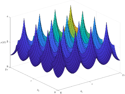
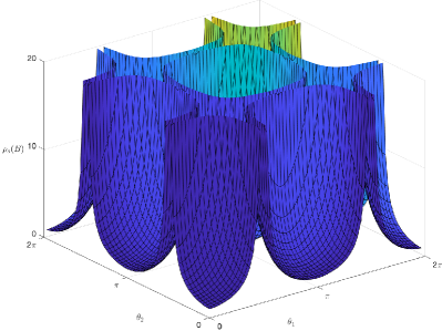
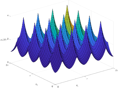
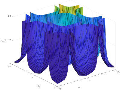
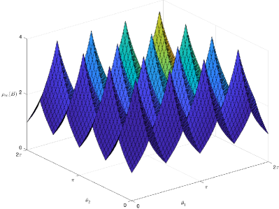
Figures 1a, 1c, and 1e show maps of $\rho(B)$, $\rho_{o}(B)$, and $\rho_{\infty}(B)$ using GENP for $B=B(\theta_{1},\theta_{2})\in\operatorname{B}_{s}(4)$, mapped against the input angles used to generate $B$. Note the singularity lines in Figures 1a, 1c, and 1e account for when $\theta_{i}=\pi\pm\frac{\pi}{2}$ for some $i$. These coincide with when $B_{11}=\cos\theta_{1}\cos\theta_{2}=0$ and GENP factorization fails on the first step (and in fact this shows this is the only step on which GENP can fail). Figures 1b, 1d, and 1f show maps of $\rho(B)$, $\rho_{o}(B)$, and $\rho_{\infty}(B)$ using GEPP (or GERP) for $B=B(\theta_{1},\theta_{2})\in\operatorname{B}_{s}(4)$. Note each of the peaks in Figures 1b, 1d, and 1f occur precisely at the scaled Hadamard matrices, $B(\boldsymbol{\theta})\in\operatorname{B}_{s}(N)$ for $\boldsymbol{\theta}\in(\frac{\pi}{4}+\frac{\pi}{2}\mathbb{Z})^{n}$ so that $\sqrt{N}B(\boldsymbol{\theta})\in\{\pm 1\}^{N\times N}$ with orthogonal rows and columns. As such, butterfly models can be used as a continuous approximation of Hadamard matrices to derive other desirable properties. Hadamard matrices then are extreme points for these butterfly models with respect to growth factors. Walsh(-Hadamard) transformations are a popular choice to efficiently randomize the elements of a matrix [19]. With respect to the growth factor, then Walsh transforms appear to be the least desirable preconditioners in the butterfly ensembles. This will be explored further in future work.

The relationship $1\leq\rho(B)\leq\rho_{\infty}(B)$ can easily be viewed for this case, as Figure 1a fits inside Figure 1e and Figure 1b fits inside Figure 1f. Similarly, the relationships to $\rho_{o}(B)$ using GEPP can be viewed by iteratively stacking Figures 1b, 1d, and 1f

2.1.2 Numerical experiments

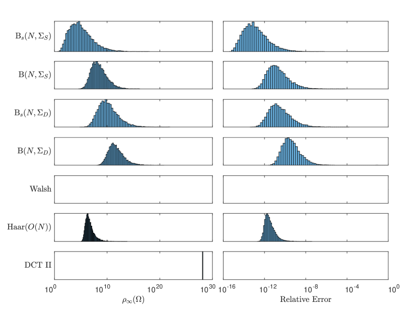
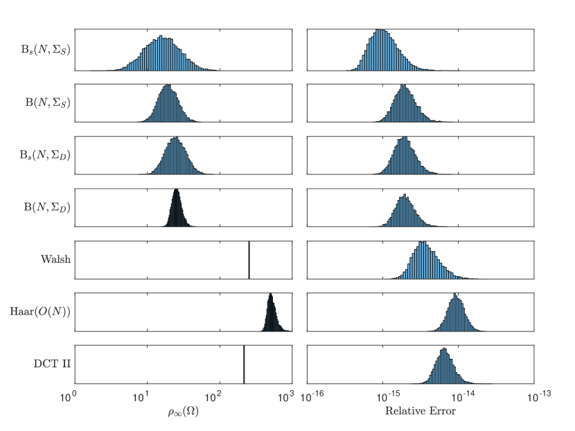
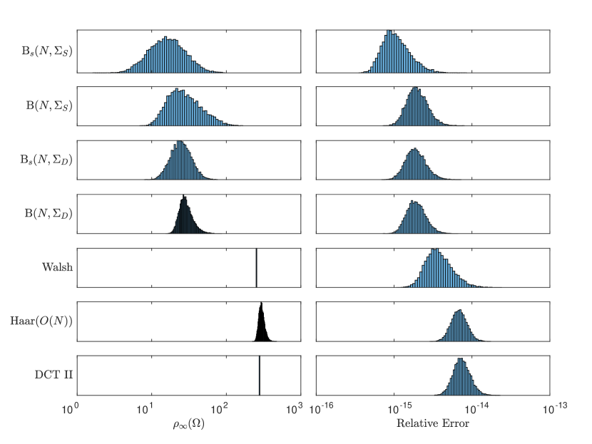
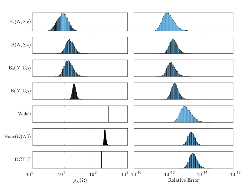
In this section, we will run numerical experiments to compare the impact on the growth factor and relative errors in the naïve model when using a variety of random preconditioners $\Omega$ with GENP, GEPP, GERP, and GECP. These will only include the 1-sided transformations, so that the growth factors of the preconditioning matrices can be explored directly. Experiments are run using MATLAB in double precision, where $\epsilon=2^{-52}$ ($\epsilon\approx 2.220446\cdot 10^{-16})$. We will run $10,000$ trials for each preconditioner for the naïve model ${\mathbf{I}}{\mathbf{x}}={\mathbf{b}}$, where ${\mathbf{x}}\sim\operatorname{Uniform}(\mathbb{S}^{N-1})$ and $N=2^{n}$ for $n=2$ to $n=8$. To ease the following discussion, we choose $N=2^{8}$ as we feel it is representative of the performance we observed for other choices of $N$. For computational simplicity, we will only consider $\rho_{\infty}$. Additionally, one step of iterative refinement will be run. Tables 1, 2, 3, and 4 will show the sample medians, means ($\bar{x}$) and standard deviations ($s$) for the trials for $n=8$. Moreover, Figures 2, 3, 4, and 5 will summarize the growth factors and relative errors, resp. $\rho_{\infty}(\Omega)$ and $\frac{\|{\mathbf{x}}-\hat{{\mathbf{x}}}\|_{\infty}}{\|{\mathbf{x}}\|_{\infty}}$.

The particular random preconditioners we will use in these experiments are

• $\operatorname{B}_{s}(N,\Sigma_{S})$

• $\operatorname{B}(N,\Sigma_{S})$

• $\operatorname{B}_{s}(N,\Sigma_{D})$

• $\operatorname{B}(N,\Sigma_{D})$

• Walsh transform

• $\operatorname{Haar}(\operatorname{O}(N))$

• Discrete Cosine Transform (DCT II).

See Section 1.2 for more information on the Walsh, Haar orthogonal and DCT transformations.

Remark 2.14.

The parameters needed to generate each butterfly matrix (i.e., the number of uniform angles) increases from $n$ for $\operatorname{B}_{s}(N,\Sigma_{S})$, $N-1$ for both $\operatorname{B}(N,\Sigma_{S})$ and $\operatorname{B}_{s}(N,\Sigma_{D})$, to $\frac{1}{2}Nn$ for $\operatorname{B}_{s}(N,\Sigma_{D})$. The ordering of the butterfly models included in the summary tables and figures reflects this increasing of number of these parameters. These compare to $\binom{N}{2}=\frac{1}{2}N(N-1)$ uniform angles that could be used to sample $\operatorname{Haar}(\operatorname{O}(N))$, which can be realized by using Givens rotations to find the $QR$ factorization of $\operatorname{Gin}(N,N)$.

	Growth factor: $\rho_{\infty}$			Relative error			Relative error + Iterative refinement
	Median	$\bar{x}$	$s$	Median	$\bar{x}$	$s$	Median	$\bar{x}$	$s$
$\operatorname{B}_{s}(N,\Sigma_{S})$	5.18e+04	5.09e+14	5.08e+16	1.00e-13	6.78e-10	6.43e-08	4.07e-16	4.15e-16	8.86e-17
$\operatorname{B}(N,\Sigma_{S})$	1.95e+08	1.16e+13	5.95e+14	1.51e-11	6.48e-09	3.85e-07	4.08e-16	4.18e-16	1.48e-16
$\operatorname{B}_{s}(N,\Sigma_{D})$	1.03e+10	1.17e+19	1.13e+21	2.39e-11	1.38e-01	1.38e+01	4.10e-16	2.40e-03	2.37e-01
$\operatorname{B}(N,\Sigma_{D})$	3.00e+11	1.43e+16	5.32e+17	3.16e-10	1.65e-01	7.58e+00	4.06e-16	5.29e-10	4.17e-08
Walsh	NaN	NaN	NaN	NaN	NaN	NaN	NaN	NaN	NaN
$\operatorname{Haar}(\operatorname{O}(N))$	3.27e+06	2.68e+09	1.05e+11	2.61e-12	1.12e-11	8.54e-11	1.04e-15	1.07e-15	2.12e-16
DCT II	1.33e+28	1.33e+28	0.00e+00	4.33e+12	5.48e+12	4.61e+12	3.89e+14	4.94e+14	4.16e+14

Table 1: Naïve model numerical experiments for GENP with 10,000 trials for $N=2^{8}$

	Growth factor: $\rho_{\infty}$			Relative error			Relative error + Iterative refinement
	Median	$\bar{x}$	$s$	Median	$\bar{x}$	$s$	Median	$\bar{x}$	$s$
$\operatorname{B}_{s}(N,\Sigma_{S})$	1.60e+01	1.87e+01	1.11e+01	1.00e-15	1.15e-15	5.72e-16	4.07e-16	4.16e-16	9.11e-17
$\operatorname{B}(N,\Sigma_{S})$	1.93e+01	2.02e+01	6.19e+00	1.94e-15	2.07e-15	6.91e-16	4.07e-16	4.16e-16	8.82e-17
$\operatorname{B}_{s}(N,\Sigma_{D})$	2.42e+01	2.58e+01	8.64e+00	1.91e-15	2.04e-15	6.85e-16	4.09e-16	4.18e-16	8.73e-17
$\operatorname{B}(N,\Sigma_{D})$	2.54e+01	2.59e+01	3.87e+00	1.96e-15	2.08e-15	6.58e-16	4.07e-16	4.15e-16	8.94e-17
Walsh	2.56e+02	2.56e+02	0.00e+00	3.66e-15	4.09e-15	1.86e-15	3.28e-16	3.35e-16	6.02e-17
$\operatorname{Haar}(\operatorname{O}(N))$	5.20e+02	5.32e+02	7.52e+01	9.27e-15	9.59e-15	2.42e-15	1.04e-15	1.07e-15	2.10e-16
DCT II	2.14e+02	2.14e+02	1.85e-12	6.56e-15	6.86e-15	1.92e-15	3.48e-16	3.54e-16	6.02e-17

Table 2: Naïve model numerical experiments for GEPP with 10,000 trials for $N=2^{8}$

	Growth factor: $\rho_{\infty}$			Relative error			Relative error + Iterative refinement
	Median	$\bar{x}$	$s$	Median	$\bar{x}$	$s$	Median	$\bar{x}$	$s$
$\operatorname{B}_{s}(N,\Sigma_{S})$	1.60e+01	1.87e+01	1.11e+01	1.02e-15	1.17e-15	5.69e-16	4.06e-16	4.17e-16	9.28e-17
$\operatorname{B}(N,\Sigma_{S})$	2.59e+01	3.12e+01	1.79e+01	1.95e-15	2.08e-15	6.78e-16	4.06e-16	4.16e-16	8.96e-17
$\operatorname{B}_{s}(N,\Sigma_{D})$	2.45e+01	2.59e+01	8.36e+00	1.87e-15	1.99e-15	6.31e-16	4.08e-16	4.18e-16	9.08e-17
$\operatorname{B}(N,\Sigma_{D})$	2.81e+01	2.95e+01	6.78e+00	1.90e-15	2.00e-15	5.94e-16	4.07e-16	4.17e-16	8.99e-17
Walsh	2.56e+02	2.56e+02	0.00e+00	3.64e-15	4.11e-15	1.89e-15	3.28e-16	3.34e-16	6.00e-17
$\operatorname{Haar}(\operatorname{O}(N))$	2.96e+02	3.00e+02	2.77e+01	6.80e-15	7.01e-15	1.68e-15	1.04e-15	1.07e-15	2.11e-16
DCT II	2.79e+02	2.79e+02	5.63e-12	7.32e-15	7.65e-15	2.04e-15	3.48e-16	3.54e-16	6.13e-17

Table 3: Naïve model numerical experiments for GERP with 10,000 trials for $N=2^{8}$

	Growth factor: $\rho_{\infty}$			Relative error			Relative error + Iterative refinement
	Median	$\bar{x}$	$s$	Median	$\bar{x}$	$s$	Median	$\bar{x}$	$s$
$\operatorname{B}_{s}(N,\Sigma_{S})$	8.90e+00	9.44e+00	3.54e+00	1.08e-15	1.22e-15	5.77e-16	4.08e-16	4.18e-16	9.10e-17
$\operatorname{B}(N,\Sigma_{S})$	1.50e+01	1.57e+01	4.63e+00	1.56e-15	1.64e-15	4.75e-16	4.06e-16	4.15e-16	8.75e-17
$\operatorname{B}_{s}(N,\Sigma_{D})$	1.35e+01	1.46e+01	5.20e+00	1.34e-15	1.43e-15	4.49e-16	4.08e-16	4.18e-16	8.95e-17
$\operatorname{B}(N,\Sigma_{D})$	2.06e+01	2.09e+01	2.70e+00	1.73e-15	1.81e-15	4.76e-16	4.07e-16	4.15e-16	8.72e-17
Walsh	2.56e+02	2.56e+02	0.00e+00	3.66e-15	4.09e-15	1.86e-15	3.28e-16	3.35e-16	6.02e-17
$\operatorname{Haar}(\operatorname{O}(N))$	1.93e+02	1.95e+02	1.35e+01	5.43e-15	5.61e-15	1.35e-15	1.04e-15	1.07e-15	2.12e-16
DCT II	7.65e+01	7.31e+01	1.09e+01	6.15e-15	6.46e-15	1.84e-15	3.49e-16	3.55e-16	6.16e-17

Table 4: Naïve model numerical experiments for GECP with 10,000 trials for $N=2^{8}$

Figure 2: Naïve model: $\rho_{\infty}$ and relative errors using GENP, $N=2^{8}$, 10,000 trials

Figure 3: Naïve model: $\rho_{\infty}$ and relative errors using GEPP, $N=2^{8}$, 10,000 trials

Figure 4: Naïve model: $\rho_{\infty}$ and relative errors using GERP, $N=2^{8}$, 10,000 trials

Figure 5: Naïve model: $\rho_{\infty}$ and relative errors using GECP, $N=2^{8}$, 10,000 trials

2.1.3 Discussion

For the naïve model, note the Walsh matrix used by MATLAB has leading $2\times 2$ subblock of the form $\begin{bmatrix}1&1\\ 1&1\end{bmatrix}$. Hence, GENP will stop after one step of GE since the second pivot is 0. So for this model, the Walsh transform fails for the GENP experiments, and so does not produce any data used in Tables 1 and 2. Although the DCT matrix used by MATLAB has nonvanishing principal minors, small pivots are introduced very early in GENP (e.g., $U_{22}=-1.3311\cdot 10^{-5}$) so the resulting factorization has a very large growth factor, where the computed $\widehat{\rho}_{\infty}=1.3254\cdot 10^{28}$ (as seen in Table 1). Using GENP, DCT results in very large relative errors not included in the scaling of Figure 2.

In line with Corollary 2.8, $\rho_{\infty}(B)$ then will look progressively lognormal for $B\sim\operatorname{B}(N,\Sigma_{S})$. It happens this behavior seems universal for other butterfly models as well as $\operatorname{Haar}(\operatorname{O}(N))$. This aligns partially with an observation of Trefethen and Schreiber in the iid model cases, which showed near universal behavior that could be modeled by $\operatorname{Gin}(N,N)$ since only a few steps of GE resulted in near Gaussian entries [20]. We note also how the supports for the Haar-butterfly and Haar orthogonal $\ell_{\infty}$-growth factors when using GEPP are essentially disjoint in Figure 3. This aligns with Eq. 23, so that $n=8$ appears to be large enough to exhibit this behavior.

Overall for GENP, the butterfly models have moderate growth factors and relative errors, with the one step of iterative refinement essentially correcting the propagated errors introduced by (unnecessarily) using GE to solve the naïve model. Surprisingly, the simplest butterfly model $\operatorname{B}_{s}(N,\Sigma_{S})$ did the least damage among the preconditioners in the GENP experiments. $\operatorname{Haar}(\operatorname{O}(N))$ outperformed the remaining butterfly models. For GEPP, GERP, and GECP, the butterfly models outperformed the remaining models (i.e., they did the least damage) while the Walsh transformation outperformed both the DCT $\operatorname{Haar}(\operatorname{O}(N))$ transformations, with DCT having smaller errors than $\operatorname{Haar}(\operatorname{O}(N))$ only in the GEPP case.

In comparing different pivoting strategies, one sees that GENP when combined with one step of iterative refinement outperforms (in terms of relative errors) the GECP relative error experiments and were on par with the GECP and one step of iterative refinement combination. In line with the purpose of the naïve model, these suggest the Haar-butterfly transformations do the least damage when solving the trivial linear system. Additionally, the added computational costs needed to run GECP seemed to go to waste, since GEPP had equivalent performance in conjunction with $\operatorname{B}_{s}(N,\Sigma_{S})$.

Remark 2.15.

Also, we can connect the prior experiments to the theoretical results from Section 2.1.1. Notably, our experiments align with the result in Theorem 2.3 that Haar-butterfly matrices have identical GEPP and GERP factorizations, as Figures 3 and 4 as well as Tables 2 and 3 both support. Moreover, using Theorem 2.3, we can compute the mean and the standard deviation for $\rho_{\infty}(B)$ exactly for GEPP and GERP for $B\sim\operatorname{B}_{s}(N,\Sigma_{S})$: in both cases, we have $\mathbb{E}\rho_{\infty}(B)=N^{\gamma}=\left(1+\frac{\log 4}{\pi}\right)^{8}\approx 18.619399429$ for $N=2^{8}$ (cf. Corollary 2.7) and a similar computation yields

(30) $$\operatorname{Var}\rho_{\infty}(B)=\left(4\cdot\frac{1+\log 2}{\pi}\right)^{8}-\left(1+\frac{\log 4}{\pi}\right)^{16}\approx 119.803995751$$

so that the population standard deviation is $\sigma_{\rho_{\infty}(B)}=\sqrt{\operatorname{Var}\rho_{\infty}(B)}\approx 10.9455011649$. These essentially match the respective sample mean and standard deviation computations of 18.7152 and 11.1003 from Table 2 and 18.6695 and 11.058 from Table 3.

Next, we can connect the theoretical and numerical median estimates for Haar-butterfly matrices. Since we are scaling the axis to show logarithmic growth factors, the middle of the then approximate Gaussian curves aligns with the median rather than the average of $\rho_{\infty}$ for both the GENP (when the average is actually infinite) and GEPP (and GERP) experiments. Additionally, in line with Corollary 2.10 where we showed the median of the max-norm growth factor, $\rho(B)$, for $B\sim\operatorname{B}_{s}(N,\Sigma_{S})$ is approximately $N^{2}$, we have $\mu_{\infty}=\mathbb{E}\ln(\rho_{\infty}(B))=\frac{2G}{\pi}+\frac{5}{4}\ln 2$ so that $\frac{\mu_{\infty}}{\ln 2}\approx 2.0912669407$ provides an approximate median, $M_{n,\infty}$, for the $\ell_{\infty}$-growth factor, $\rho_{\infty}(B)$, where $M_{n,\infty}=N^{\mu_{\infty}/\ln 2+o(n^{-1/2})}$. Figure 2 shows the marker representing $\mathbb{E}\log_{10}(\rho_{\infty}(B))=\frac{n\mu_{\infty}}{\ln 10}\approx 5.036$ (so about halfway between $10^{0}$ and $10^{10}$ in Figure 2) is not yet a good approximation for the GENP median $M_{n,\infty}$ when $n=8$ since the plot of $\rho_{\infty}(B)$ is not sufficiently lognormal: the estimate $N^{\mu_{\infty}/\ln 2}\approx 108,710$ is about twice as large as the sample median $\widehat{M}_{n}=51,776$ from Table 1. However, the GEPP and GERP plots for $\rho_{\infty}$ in Figures 3 and 4 appears much closer to lognormal than the GENP case, so $\mu_{\infty}=\frac{\ln 2}{2}$ yields the marker at $\mathbb{E}\log_{10}(\rho_{\infty}(B))=\frac{n\mu_{\infty}}{\ln 10}=\frac{4\ln 2}{\ln 10}\approx 1.20411998$ (between $10^{1}$ and $10^{2}$ in Figures 3 and 4) where $n=8$ provides a much better estimator for the median of Figures 3 and 4 using GEPP or GERP: here $10^{\frac{4\ln 2}{\ln 10}}=2^{4}=16$ provides a very good approximation for the computed sample medians 16.0059 from Table 2 and 15.987 from Table 3.

2.2 Worst-case model

Wilkinson established a weak form of backward stability of GEPP by showing $\rho(A)\leq 2^{m-1}$ for any nonsingular $A\in\mathbb{R}^{m\times m}$ [24, 25]. In [24, pg. 202], Wilkinson further shows this bound on worst-case growth factor is sharp, using the following construction:

(31) $$A_{m}={\mathbf{I}}_{m}-\sum_{i>j}{\mathbf{E}}_{ij}+\sum_{i=1}^{m-1}{\mathbf{E}}_{im}.$$

By design, GEPP would carry out without using any pivoting on $A_{m}$ at any intermediate GE steps, so that the $A_{m}=LU$ factorizations coincide for GENP and GEPP, where $L={\mathbf{I}}_{m}-\sum_{i>j}{\mathbf{E}}_{ij}$ and $U={\mathbf{I}}_{m}-{\mathbf{E}}_{mm}+\sum_{i=1}^{m}2^{i-1}{\mathbf{E}}_{im}.$ It follows $\rho(A_{m})=|U_{mm}|=2^{m-1}.$ For example,

(32) $$A_{4}=\begin{bmatrix}1&&&1\\ -1&1&&1\\ -1&-1&1&1\\ -1&-1&-1&1\end{bmatrix}=\begin{bmatrix}1\\ -1&1\\ -1&-1&1\\ -1&-1&-1&1\end{bmatrix}\begin{bmatrix}1&&&1\\ &1&&2\\ &&1&4\\ &&&8\end{bmatrix}$$

has $\rho(A_{4})=8=2^{3}$.

It happens that also $\rho_{\infty}(A_{m})=2^{m-1}$ (while $\rho_{o}(A_{m})=1+\frac{2}{m}(2^{m-1}-1)$), although this is not the upper bound of $\rho_{\infty}$. See [3] for additional discussions relating to explicit relationships and bounds between different growth factors.

Remark 2.16.

Note GECP, GERP, or any column pivoting scheme would result in $PAQ=LU$ for $P={\mathbf{I}}$ and $Q=P_{(2\ m)(3\ m)\cdots(m-1\ m)}=P_{(2\ m\ m-1\ \cdots\ 3)}$ for $L={\mathbf{I}}+\sum_{i>j\geq 2}{\mathbf{E}}_{ij}-\sum_{i=2}^{m}{\mathbf{E}}_{ij}$ and $U={\mathbf{E}}_{11}+2{\mathbf{E}}_{22}-2\sum_{i=3}^{m}{\mathbf{E}}_{ii}+\sum_{i=1}^{m-1}{\mathbf{E}}_{i,i+1}$, where $\rho(A)=2$ (while $\rho_{o}(A_{m})=3-\frac{2}{m}$ and $\rho_{\infty}(A_{m})=3-\delta_{m2}$). For example,

(33) $$A_{4}P_{(2\ 4\ 3)}=\begin{bmatrix}1&1\\ -1&1&1\\ -1&1&-1&1\\ -1&1&-1&-1\end{bmatrix}=\begin{bmatrix}1\\ -1&1\\ -1&1&1\\ -1&1&1&1\end{bmatrix}\begin{bmatrix}1&1\\ &2&1\\ &&-2&1\\ &&&-2\end{bmatrix}.$$

In particular, we see GE with column partial pivoting leads to very small growth factors for the Wilkinson model. This aligns with the observation by Cortéz and Peña that matrices appearing in practical observations for which the (row) GEPP growth factors are very large then have small growth factors when using partial pivoting by columns [3].

Remark 2.17.

Figure 6: $\ell_{2}$-relative error using GENP or GEPP to solve $A_{N}{\mathbf{x}}={\mathbf{b}}$ with ${\mathbf{x}}\sim\operatorname{Uniform}(\mathbb{S}^{N-1})$, $10^{6}$ trials for $N=2^{6}$

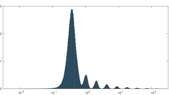
Using GENP or GEPP with $A_{N}$ (which are equivalent for this matrix), accuracy is lost very quickly when using double precision. A direct computation shows $\kappa_{\infty}(A_{N})=N$, so the relative error upper bound in Eq. 6 is

(34) $$4N^{2}\kappa_{\infty}(A_{N})\rho(A_{N})\epsilon=4N^{3}2^{N-1}\epsilon=2^{2+3n+N-1-52}=2^{2^{n}+3n-51}.$$

Since $2^{n}+3n-51<0$ for $n<17-\frac{W(131072\ln(2)/3)}{\ln 2}\approx 5.151584709$ (using the Lambert $W$ function), then the relative errors can exceed 1 for $n\geq 6$. The instability of computed solutions in these scenarios can lead to interesting distributions. For example, Figure 6 shows the resulting summary image for $n=6$ of the $\ell_{2}$-relative error, $\frac{\|{\mathbf{x}}-\hat{{\mathbf{x}}}\|_{2}}{\|{\mathbf{x}}\|_{2}}$, running $10^{6}$ trials using GENP (or GEPP) to solve $A_{N}{\mathbf{x}}={\mathbf{b}}$ for ${\mathbf{x}}\sim\operatorname{Uniform}(\mathbb{S}^{N-1})$.

Remark 2.18.

Unlike in the naïve model, establishing the exact distributional properties of $UA_{N}V^{*}$ for iid $U,V\sim\operatorname{B}_{s}(N,\Sigma_{S})$ is not as tractable since the worst case model loses the Kronecker product forms. One would need to apply the 2-sided Haar-butterfly transform to a Kronecker product matrix to be able to yield full distributional descriptions like in Theorem 2.3 (which through the invariance properties of the Haar measure equivalently uses $UAV^{*}$ for $A={\mathbf{I}}_{N}$, which can be realized as the $n$-fold Kronecker product of ${\mathbf{I}}_{2}$).

2.2.1 Numerical experiments

For the worst-case model, our goal is to better understand how much of a dampening effect preconditioning by butterfly matrices can have. We will study the two-sided preconditioning by looking at models as outlined in (2) when studying the linear system $A_{N}{\mathbf{x}}={\mathbf{b}}$ for ${\mathbf{x}}\sim\operatorname{Uniform}(\mathbb{S}^{N-1})$ for $N=2^{n}$ and $n=2$ to 8. We are again running $10,000$ trials computing $\rho_{\infty}$, relative errors and relative errors after one step of iterative refinement for GENP, GEPP, GERP, and GECP. Hence, we are starting with a linear system with a maximal growth factor $\rho$, and we will study how the growth factor and the corresponding relative error of computed solutions are impacted through using GE to solve the equivalent linear systems

(35) $$UA_{N}V^{*}{\mathbf{y}}=U{\mathbf{b}}\quad\mbox{and}\quad{\mathbf{x}}=V^{*}{\mathbf{y}}$$

for independent random transformations $U,V$. For computational simplicity, we will compare $\rho_{\infty}$, for which we note $\rho_{\infty}(A_{N})=\rho(A_{N})=2^{N-1}$, using the same random transformations used in Section 2.1.2: $\operatorname{B}_{s}(N,\Sigma)$ and $\operatorname{B}(N,\Sigma)$ for $\Sigma=\Sigma_{S}$ and $\Sigma_{D}$, along with the Walsh transform, Haar orthogonal transform and Discrete Cosine Transform. (See Sections 1.2 and 2.1.2 for more explicit descriptions of the transformations used in these experiments.) Tables 5, 6, 7, and 8 will summarize the sample medians, means and standard deviations for the $n=8$ trials.

	Growth factor: $\rho_{\infty}$			Relative error			Relative error + Iterative refinement
	Median	$\bar{x}$	$s$	Median	$\bar{x}$	$s$	Median	$\bar{x}$	$s$
$\operatorname{B}_{s}(N,\Sigma_{S})$	3.30e+05	1.93e+13	1.93e+15	2.20e-12	9.10e-10	5.72e-08	2.60e-15	2.87e-15	1.24e-15
$\operatorname{B}(N,\Sigma_{S})$	3.16e+05	9.33e+08	5.51e+10	2.87e-12	3.71e-11	1.78e-09	2.74e-15	2.92e-15	9.17e-16
$\operatorname{B}_{s}(N,\Sigma_{D})$	4.04e+05	3.45e+09	1.94e+11	3.32e-12	3.16e-11	9.37e-10	2.64e-15	2.86e-15	1.11e-15
$\operatorname{B}(N,\Sigma_{D})$	2.27e+05	2.10e+10	1.93e+12	2.33e-12	6.63e-06	6.56e-04	2.78e-15	7.69e-14	7.39e-12
Walsh	1.86e+28	7.38e+42	7.19e+44	8.63e+00	1.60e+12	4.37e+13	8.16e-01	6.33e+16	6.15e+18
$\operatorname{Haar}(\operatorname{O}(N))$	2.17e+05	2.30e+08	1.10e+10	1.99e-12	8.88e-12	6.98e-11	7.73e-15	8.05e-15	1.89e-15
DCT II	3.91e+05	7.16e+08	3.34e+10	6.38e-12	2.06e-09	1.90e-07	2.57e-15	5.40e-15	2.74e-13

Table 5: Worst-case model numerical experiments for GENP with 10,000 trials for $N=2^{8}$ (excluding 505 Walsh trials where GENP failed)

	Growth factor: $\rho_{\infty}$			Relative error			Relative error + Iterative refinement
	Median	$\bar{x}$	$s$	Median	$\bar{x}$	$s$	Median	$\bar{x}$	$s$
$\operatorname{B}_{s}(N,\Sigma_{S})$	2.67e+01	2.97e+01	1.51e+01	6.85e-15	8.94e-15	8.81e-15	2.59e-15	2.89e-15	1.27e-15
$\operatorname{B}(N,\Sigma_{S})$	5.66e+01	5.79e+01	1.53e+01	8.75e-15	9.38e-15	3.45e-15	2.75e-15	2.92e-15	9.17e-16
$\operatorname{B}_{s}(N,\Sigma_{D})$	5.20e+01	5.17e+01	1.07e+01	7.11e-15	7.93e-15	3.90e-15	2.64e-15	2.87e-15	1.10e-15
$\operatorname{B}(N,\Sigma_{D})$	7.09e+01	6.90e+01	1.23e+01	8.16e-15	8.47e-15	2.09e-15	2.77e-15	2.93e-15	8.87e-16
Walsh	7.46e+01	7.17e+01	1.16e+01	8.36e-15	8.60e-15	1.97e-15	1.99e-15	2.11e-15	6.83e-16
$\operatorname{Haar}(\operatorname{O}(N))$	7.47e+01	7.19e+01	1.13e+01	1.09e-14	1.11e-14	2.29e-15	7.73e-15	8.05e-15	1.91e-15
DCT II	7.65e+01	7.31e+01	1.09e+01	8.45e-15	8.68e-15	1.90e-15	2.57e-15	2.67e-15	6.82e-16

Table 6: Worst-case model numerical experiments for GEPP with 10,000 trials for $N=2^{8}$

	Growth factor: $\rho_{\infty}$			Relative error			Relative error + Iterative refinement
	Median	$\bar{x}$	$s$	Median	$\bar{x}$	$s$	Median	$\bar{x}$	$s$
$\operatorname{B}_{s}(N,\Sigma_{S})$	2.59e+01	2.66e+01	6.96e+00	3.05e-15	3.22e-15	9.63e-16	2.59e-15	2.88e-15	1.26e-15
$\operatorname{B}(N,\Sigma_{S})$	5.33e+01	5.27e+01	1.14e+01	4.72e-15	4.88e-15	1.31e-15	2.75e-15	2.92e-15	9.09e-16
$\operatorname{B}_{s}(N,\Sigma_{D})$	3.85e+01	3.85e+01	6.42e+00	3.16e-15	3.29e-15	8.73e-16	2.63e-15	2.84e-15	1.09e-15
$\operatorname{B}(N,\Sigma_{D})$	6.12e+01	5.99e+01	6.67e+00	5.13e-15	5.27e-15	1.16e-15	2.76e-15	2.93e-15	8.90e-16
Walsh	7.34e+01	7.32e+01	4.19e+00	5.52e-15	5.64e-15	1.16e-15	1.98e-15	2.10e-15	6.78e-16
$\operatorname{Haar}(\operatorname{O}(N))$	7.32e+01	7.29e+01	4.36e+00	9.28e-15	9.55e-15	2.02e-15	7.73e-15	8.05e-15	1.93e-15
DCT II	7.33e+01	7.30e+01	4.26e+00	5.75e-15	5.86e-15	1.16e-15	2.56e-15	2.67e-15	6.81e-16

Table 7: Worst-case model numerical experiments for GERP with 10,000 trials for $N=2^{8}$

	Growth factor: $\rho_{\infty}$			Relative error			Relative error + Iterative refinement
	Median	$\bar{x}$	$s$	Median	$\bar{x}$	$s$	Median	$\bar{x}$	$s$
$\operatorname{B}_{s}(N,\Sigma_{S})$	1.36e+01	1.44e+01	4.69e+00	2.71e-15	2.87e-15	8.61e-16	2.52e-15	2.81e-15	1.31e-15
$\operatorname{B}(N,\Sigma_{S})$	4.17e+01	4.18e+01	9.74e+00	3.80e-15	3.94e-15	1.05e-15	2.62e-15	2.86e-15	1.18e-15
$\operatorname{B}_{s}(N,\Sigma_{D})$	1.88e+01	1.92e+01	4.10e+00	2.68e-15	2.84e-15	8.14e-16	2.45e-15	2.70e-15	1.23e-15
$\operatorname{B}(N,\Sigma_{D})$	4.66e+01	4.58e+01	4.92e+00	3.93e-15	4.06e-15	9.14e-16	2.63e-15	2.87e-15	1.20e-15
Walsh	6.46e+01	6.46e+01	2.99e+00	4.57e-15	4.66e-15	9.37e-16	2.10e-15	2.23e-15	8.00e-16
$\operatorname{Haar}(\operatorname{O}(N))$	6.43e+01	6.43e+01	3.10e+00	8.76e-15	9.03e-15	1.93e-15	5.87e-15	6.30e-15	1.92e-15
DCT II	6.44e+01	6.44e+01	3.03e+00	4.85e-15	4.95e-15	9.77e-16	2.33e-15	2.48e-15	8.11e-16

Table 8: Worst-case model numerical experiments for GECP with 10,000 trials for $N=2^{8}$

Figure 7: Worst-case model: $\rho_{\infty}$ and relative errors using GENP, $N=2^{8}$, 10,000 trials

Figure 8: Worst-case model: $\rho_{\infty}$ and relative errors using GEPP, $N=2^{8}$, 10,000 trials

Figure 9: Worst-case model: $\rho_{\infty}$ and relative errors using GERP, $N=2^{8}$, 10,000 trials

Figure 10: Worst-case model: $\rho_{\infty}$ and relative errors using GECP, $N=2^{8}$, 10,000 trials

2.2.2 Discussion

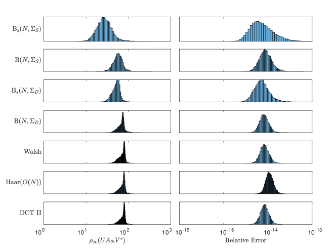
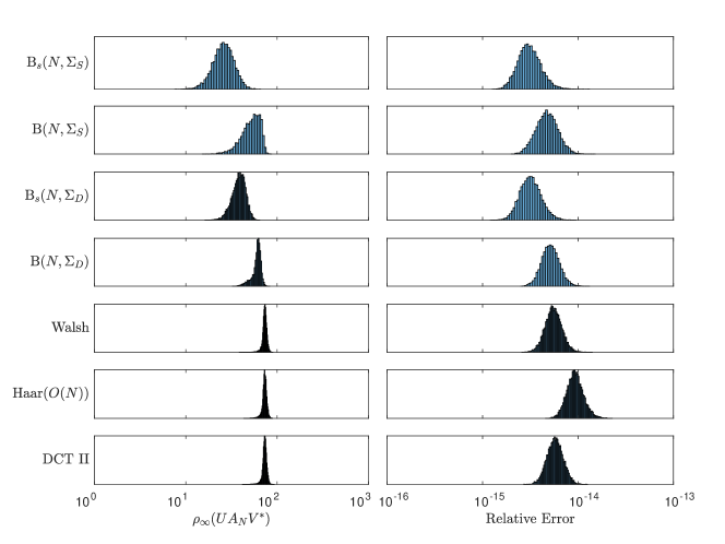
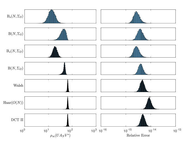
Recall using GEPP (or GENP), we have $\rho_{\infty}(A_{N})=2^{N-1}$. In particular, for $n=8$ then $\rho_{\infty}(A_{N})=2^{255}\approx 5.7896\cdot 10^{76}$. Table 6 shows each random preconditioner has beneficial dampening impacts in terms of reducing the growth factors and the associated relative errors. Figure 8 further illustrates this dampening impact with respect to the growth factors. Each preconditioner has growth factor approximately less than $10^{2}$, far away from the worst-case scenario.

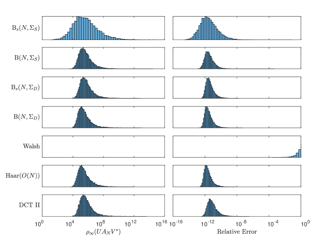
Using GENP, all except the Walsh transform have strong dampening impacts on the growth factor, as illustrated in Table 5 and Figure 7. Of interest for the Walsh transform is that the resulting matrix $UA_{N}V^{*}$ can now be block degenerate. For our 10,000 trials, 505 using the Walsh transform resulted in block degenerate matrices. (Table 5 shows the summary of the results for the block nondegenerate trials.) Overall, even when the transformed matrix was block nondegenerate, the results were nowhere near the performance seen in the other random preconditioners considered and led to highly unstable computed solutions. Using GENP, the Haar orthogonal transformations had the best performance on average, while the butterfly models still outperformed the DCT. Among the butterfly models, $\operatorname{B}(N,\Sigma_{S})$ and $\operatorname{B}_{s}(N,\Sigma_{D})$ had the smallest growth factors and best precision results. Adding one step of iterative refinement then led to also $\operatorname{B}_{s}(N,\Sigma_{S})$ matching precision of the GEPP, GERP, and GECP experiments. Note also that although $\operatorname{B}_{s}(N,\Sigma_{S})$ had a larger average relative error than most of the other models, its median was smaller than all but the Haar orthogonal case. Moreover, comparing the histograms in Figure 7 indicates about a fifth of the time the relative error for GENP is smaller than the left edge of the bulk for each of the remaining models. So even though the Haar-butterfly models led to some samples with the largest relative errors (excluding the Walsh model), they also produced a portion of samples that had higher accuracy than any other model.

For the GERP and GECP experiments, the worst-case model actual is closer in spirit to the naïve model since $\rho_{\infty}(A_{N})=3$ is almost optimal. So these experiments measure how much this preconditioning can mess things up. In this light, all of the butterfly models outperformed the remaining random transformations.

Also of note with respect to the $\operatorname{B}_{s}(N,\Sigma_{S})$ trials is that the logarithmic growth factors in Figure 7 both look approximately lognormal, while the $\operatorname{Haar}(\operatorname{O}(N))$ logarithmic growth factor generates a non-lognormal histogram, especially in the GEPP case. The remaining butterfly models lie in between and appear to resemble interpolations between these two models.

2.3 Conclusions

While Parker had shown one could remove the need of pivoting in GE through the use of butterfly matrices (see Theorem 1.1), we wanted to explore whether this was a good idea in practice. In spite of the benefits one can gain in reducing computation time, one could lose stability when removing pivoting with GE. This idea had been explored previously in [13], where the authors ran experiments using a combination of butterfly transformations and one step of iterative refinement in a mixed-precision setup to establish how much stability was regained. Our results for both the naïve and worst-case models align with theirs, in that one step of iterative refinement seems necessary to stabilize computed solutions when using GENP. We additionally took the direction of comparing performance between different pivoting schemes. The added complexity needed to compute GECP over GEPP did not result in significant gains in precision. In the case of $\operatorname{B}_{s}(N,\Sigma_{S})$, GEPP had nearly identical precision in computed solutions as GECP in the naïve model. Additionally, we show that using Haar-butterfly matrices with GENP does the least damage in the trivial linear system. Although one step of iterative refinement more than corrects computed errors using only GENP, the errors are still not too extreme. Future work can also further explore mixed-precision or high precision scenarios.

Our tests also compared butterfly transformations against other transforms taken from randomized numerical linear algebra. For both the naïve and worst-case experiments using each pivoting scheme, the butterfly models achieved the highest precision results in the GEPP setup. GENP (with iterative refinement) does remain unstable, which was particularly exemplified in experiments using the Walsh transform. This does not imply no one should use Walsh transforms, since our models are purposely extreme with respect to the max-norm growth factors. In fact, the Walsh transforms do have other desirable properties not shared by the random butterfly models (such as through Hoeffding’s inequality to efficiently mix entries in a vector). For the particular setup explored in our experiments, the Walsh transform matches the worst-case growth factor behavior of the Haar-butterfly models as established in Theorem 2.3. Relationships between the Walsh transform and butterfly matrices, which can be viewed as a continuous generalization of a particular subclass of Hadamard matrices, will be further explored in future work.

Of note is Theorem 2.3, which gives the full distribution of the random growth growth factors for Haar-butterfly matrices using GENP, GEPP and GERP. This is a substantial advancement in the understanding of random growth factors for dense matrices, which had previously focused on empirical first moment estimates and asymptotic bounds for certain cases (see [20, 10]). Future work will explore whether this result can be extended to GECP.

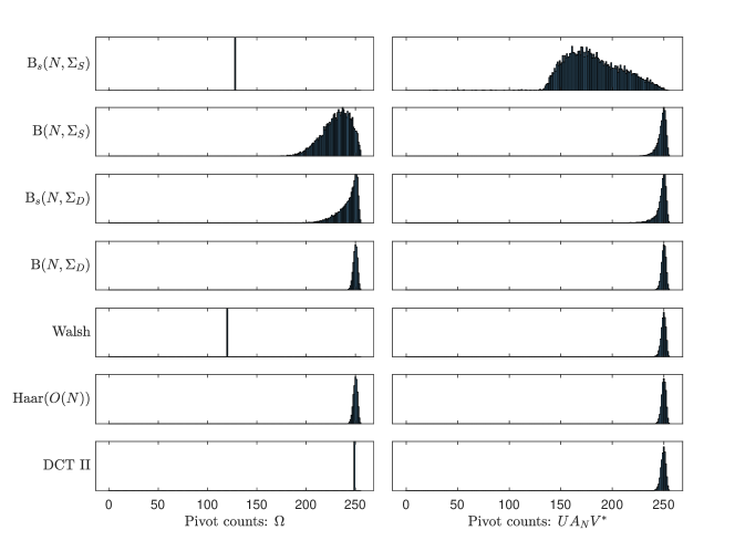
A related question that will be explored further in a future work regards the number of pivot movements these transformations yield using different pivoting strategies. Parker’s original motivation was to provide a means to remove the need for pivoting all together when using GE. Reducing the number of pivot movements would be beneficial for high performance machines to limit the communication overhead for coordinating data movements [2, 16]. Our current article explored further the implication of maintaining different pivoting strategies in addition to using these random transformations. So a natural future question is to ask how much actual data movement is there under these transformations. Figures 11 and 9 show summaries of the actual pivot movements when using GEPP for our experiments from Sections 2.1 and 2.2. Both models used matrices that would use no pivot movements with GEPP, so this study is akin to the naïve setting, by looking at how much additional movement is being introduced through these transformations. In the worst case model, only the Haar-butterfly transformation had pivot movements that were not near the upper bound for $N-1=255$. In the naïve model setting, the Haar-butterfly and Walsh transforms maintained movements no larger than $N/2=128$. The theory and numerical results for GEPP data movements will be further extended in a future study.

Figure 11: GEPP pivot movements using the naïve and worst case models, using $N=2^{8}$ and 10,000 trials

	Pivot counts: $\Omega$			Pivot counts: $UA_{N}V^{*}$
	Median	$\bar{x}$	$s$	Median	$\bar{x}$	$s$
$\operatorname{B}_{s}(N,\Sigma_{S})$	128	127.56	7.45	179	181.96	27.13
$\operatorname{B}(N,\Sigma_{S})$	232	230.31	14.25	249	247.97	4.29
$\operatorname{B}_{s}(N,\Sigma_{D})$	245	242.01	10.38	249	247.50	5.57
$\operatorname{B}(N,\Sigma_{D})$	250	249.86	2.13	250	249.89	2.11
Walsh	120	120	0	250	249.66	2.27
$\operatorname{Haar}(\operatorname{O}(N))$	250	249.88	2.11	250	249.82	2.13
DCT II	249	249	0	250	249.42	2.35

Table 9: Pivot counts for numerical experiments for GEPP with 10,000 trials for $N=2^{8}$

Another direction for future work in regards to the impact of preconditioning linear systems by random transformations can explore non-extreme models. Our two models, the naïve and worst-case, initiate with a linear systems whose growth factors, respectively, minimize and maximize the GEPP max-norm growth factor $\rho$. These extreme models can further be explored by using ensembles of random matrices with small and large growth factors. For instance, a general structure of matrices with maximal GEPP growth fact is given in [9], and can be used to design random ensembles with maximal growth factor $\rho=2^{N-1}$.

Appendix A Linear algebra background

Define $A\oplus B\in\mathbb{R}^{(n_{1}+n_{2})\times(m_{1}+m_{2})}$ to be the block diagonal matrix with blocks $A\in\mathbb{R}^{n_{1}\times m_{1}}$ and $B\in\mathbb{R}^{n_{2}\times m_{2}}$, i.e.,

(36) $$A\oplus B=\begin{bmatrix}A\\ &B\end{bmatrix}.$$

Define $A\otimes B\in\mathbb{R}^{n_{1}n_{2}\times m_{1}m_{2}}$ to be the Kronecker product of $A\in\mathbb{R}^{n_{1}\times m_{1}}$ and $B\in\mathbb{R}^{n_{2}\times m_{2}}$, given by

(37) $$A\otimes B=\begin{bmatrix}A_{11}B&\cdots&A_{1,m_{1}}B\\ \vdots&\vdots&\vdots\\ A_{n_{1},1}B&\cdots&A_{n_{1},m_{1}}B\end{bmatrix}.$$

Note $(A\otimes B)^{*}=A^{*}\otimes B^{*}$ and $(A\otimes B)^{T}=A^{T}\otimes B^{T}$. Recall $A\otimes B=P(B\otimes A)Q$ for perfect shuffle permutation matrices $P,Q$ (cf. [6]). If $A$ and $B$ are both square then $Q=P^{T}$, so that $A\otimes B$ and $B\otimes A$ are conjugate. Also, recall the mixed-product property of the Kronecker product: if the products $AC$ and $BD$ can be computed, then the product of the Kronecker products is the Kronecker product of the products, i.e.,

(38) $$(A\otimes B)(C\otimes D)=AC\otimes BD.$$

Certain classes of matrices, $\mathcal{S}$, are closed under the Kronecker product operator: if $A,B\in\mathcal{S}$ then $A\otimes B\in\mathcal{S}$. Straightforward arguments show that this holds for $\mathcal{S}$ being orthogonal, unitary, permutation, diagonal, lower-triangular or upper-triangular matrices.

The Kronecker product, in particular, allows simplified matrix norm calculations:

Lemma A.1.

If $\|\cdot\|$ is an induced $\ell^{p}$-matrix norm or $\|\cdot\|_{\max}$, then $\|A\otimes B\|=\|A\|\|B\|$ for $A\in\mathbb{R}^{n_{1}\times m_{1}}$ and $B\in\mathbb{R}^{n_{2}\times m_{2}}$.

Proof A.2.

This is a trivial calculation for $\|\cdot\|=\|\cdot\|_{\max}$. If $\|\cdot\|$ is an induced matrix norm, then the multiplicative property is established in [11, Theorem 8].

These are not the only norms on which Kronecker products satisfy this multiplicative property. Other straightforward computations show $p$-Schatten norms $|\operatorname{Tr}(A^{p})|^{1/p}$ work (since $\operatorname{Tr}(A\otimes B)=\operatorname{Tr}(A)\operatorname{Tr}(B)$ for square $A,B$), including the Frobenius norm, as well as any standard $p$-norm applied to the vectorization of the matrix $A\in\mathbb{R}^{n\times m}$ as an element of $\mathbb{R}^{nm}$ (e.g., $\|A\|_{\max}=\|\operatorname{vec}(A)\|_{\infty}$). We will restrict our attention in this paper specifically to $\|\cdot\|_{\max}$ and (the induced) $\|\cdot\|_{\infty}$.

Additionally, the Kronecker product allows for straightforward matrix factorizations determined directly from the corresponding factorizations of each factor. For example:

Lemma A.3.

If $P_{j}A_{j}Q_{j}=L_{j}U_{j}$ for permutation matrices $P_{j},Q_{j}$ and unit lower triangular $L_{j}$ and upper triangular $U_{j}$ and $\displaystyle A=\bigotimes_{j=1}^{n}A_{j}$, then $PAQ=LU$ for permutation matrices $\displaystyle P=\bigotimes_{j=1}^{n}P_{j}$, $\displaystyle Q=\bigotimes_{j=1}^{n}Q_{j}$ and unit lower triangular $\displaystyle L=\bigotimes_{j=1}^{n}L_{j}$ and upper triangular $\displaystyle U=\bigotimes_{j=1}^{n}U_{j}$.

Proof A.4.

This follows directly from the mixed-product property (38).

A.1 Gaussian elimination

Gaussian elimination (GE) remains the most prominent approach to solving linear systems $A{\mathbf{x}}={\mathbf{b}}$ for $A\in\mathbb{R}^{n\times n}$. GE without pivoting (GENP), when it succeeds, results in the triangular factorization $A=LU$ for unit lower triangular $L$ with

(39) $$L_{ij}=\frac{A^{(j)}_{ij}}{A^{(j)}_{jj}}$$

for $i>j$, where $A^{(k)}$ denotes the matrix before the $k^{th}$ step in GENP with zeros below the first $k-1$ diagonal entries, and $U=A^{(n)}$ is upper triangular with $U_{jj}=A^{(j)}_{jj}$. GENP can be carried out in $\frac{2}{3}n^{3}+\mathcal{O}(n^{2})$ FLOPs.

If $A$ is block nondegenerate, then $A$ has an $LU$ factorization using GENP. If $A$ is block degenerate, then pivoting is necessary. Even when not essential, different pivoting schemes are often employed to control errors from using floating-point arithmetic. The most popular modified version of GE is GE with partial pivoting (GEPP). This involves an additional scan at GE step $k$ to find the entry of max norm below the diagonal of $A^{(k)}$ within the column and then a possible row swap to ensure the magnitude of the entry on the $k^{th}$ diagonal is at least as large as those below it. This results in a $PA=LU$ factorization where $P$ is a permutation matrix. By construction, the $L$ factor from GEPP satisfies

(40) $$|L_{ij}|\leq 1\quad\text{for any}\quad i>j.$$

GE with complete pivoting (GECP) involves a scan through the entire lower untriangularized remaining block of $A^{(k)}$ followed by possible row and column swaps to ensure the magnitude of the entry on the $k^{th}$ diagonal is at least as large as that of all the entries in the lower-left $(n-k+1)\times(n-k+1)$ subblock of $A^{(k)}$. This results in a $PAQ=LU$ factorization for permutation matrices $P,Q$. For this paper, we will assume a pivot search chooses the pivot with minimal taxi cab distance with respect to the row and column indices to the pivot position (i.e., the main leading diagonal entry in the remaining untriangularized subblock), prioritizing minimal row index distance over column index in the case of a tie between candidates.

GE with rook pivoting (GERP) involves iteratively scanning first through the column below the diagonal to find a max norm entry, and then within that specific row to find the max norm entry, and repeating between column and row scans, until this process completes with the candidate pivot that maximizes both its row and column. This is followed then by the associated row and column swaps to move the resulting candidate to the pivot position. The name of the pivoting scheme is derived from the limitation on the pivot scans to paths a rook piece could make in a game of chess. See [17] for further discussion regarding GERP. We will not explore additional numerical experiments for GERP beyond highlighting connections to our chosen models. Note for this paper we will assume GERP always sequences column scans before row scans at each intermediate step.

The total operational costs of these pivoting schemes differs only in the added scans to find each pivot and associated row and column swaps. $\mathcal{O}(n^{2})$ and $\mathcal{O}(n^{3})$ additional scans are needed, respectively, for GEPP and GECP, while GERP ranges from twice the GEPP complexity (with respect to added scans) to the full GECP complexity. In [17], computations with iid models show that on average the number of scans needed for GERP is $\mathcal{O}(n^{2})$ as well, typically accounting for only a factor of 3 more scans than for GEPP.

Using GENP, a standard result establishes the existence and uniqueness of an GENP $LU$ factorization. The particular form presented in [8, Theorem 9.1] is given below:

Theorem A.5.

There exists a unique $LU$ factorization of $A\in\mathbb{R}^{n\times n}$ using GENP if and only if $A_{:k,:k}$ is nonsingular for $k=1,\ldots,n-1$. If $A_{:k,:k}$ is singular for some $k<n$, an $LU$ factorization may exist but it is not unique.

With pivoting, the $LU$ factorization is sensitive to row and column permutations: If $PA=LU$ is the $LU$ factorization for $A$ using GEPP, then for $B=QA$ for another permutation matrix $Q$, then we do not necessarily have $(PQ^{T})B=LU$ using GEPP. This non-uniqueness of $LU$ factors follows in the event there are any “ties” at an intermediate GE pivot search step; in such a case, we have $|A^{(j)}_{ij}|=|A^{(j)}_{jj}|$ so that $|L_{ij}|=1$ for some $i>j$. For example, if $A=\begin{bmatrix}1&x\\ 1&y\end{bmatrix}$ and $B=P_{(1\ 2)}A=\begin{bmatrix}1&y\\ 1&x\end{bmatrix}$, then using GEPP, we have

(41) $$A=\begin{bmatrix}1&0\\ 1&1\end{bmatrix}\begin{bmatrix}1&x\\ 0&y-x\end{bmatrix}\quad\mbox{and}\quad B=\begin{bmatrix}1&0\\ 1&1\end{bmatrix}\begin{bmatrix}1&y\\ 0&x-y\end{bmatrix}.$$

When ties are avoided, GEPP results in unique $L$ and $U$ factors.

Theorem A.6.

Let $A$ be a nonsingular square matrix. Then the $L$ and $U$ factors in the GEPP factorization $PA=LU$ are invariant under row permutations on $A$ iff $|L_{ij}|<1$ for all $i>j$.

Proof A.7.

By considering $B=PA$, we can assume $P={\mathbf{I}}$. Suppose first $|L_{ij}|=1$ for some $i>j$. Let $j$ and then $i$ be minimal such that this occurs. Since $|B^{(j)}_{jj}|=|B^{(j)}_{ij}|$, then using the row transposition permutation ${(i\ j)}$ would yield a different $P_{\sigma}$ factor with $\sigma(j)\neq j$, so that $P_{\sigma}\neq{\mathbf{I}}$. The $L$ and $U$ factors must differ for $P_{\sigma}B\neq B$ by Theorem A.5. Now assume $|L_{ij}|<1$ for all $i>j$. Let $P_{\sigma}B=L^{\prime}U^{\prime}$ be another GEPP factorization of $B$ for some $\sigma\in S_{n}$. Suppose $\sigma$ is a nontrivial permutation. Let $i$ be the first non-fixed point of $\sigma$, and note then $i<\min(\sigma(i),\sigma^{-1}(i))$. Then

(42) $$|(L^{\prime})_{\sigma(i),i}|=\left|\frac{(P_{\sigma}B)^{(i)}_{\sigma(i),i}}{(P_{\sigma}B)^{(i)}_{ii}}\right|=\left|\frac{B^{(i)}_{ii}}{B^{(i)}_{\sigma^{-1}(i),i}}\right|=\frac{1}{|L_{\sigma^{-1}(i),i}|}>1.$$

This contradicts (40). It follows necessarily $\sigma$ must be the trivial permutation so that $P_{\sigma}={\mathbf{I}}$. The uniqueness of the $L$ and $U$ factors follows from Theorem A.5.

Theorem A.6 can be generalized to other pivoting strategies (e.g., GECP), such that the specific $L$ and $U$ factors are unique whenever no ties are encountered in each intermediate pivot search step.

Appendix B Proofs for Section 2.1.1

Note first using (13) then we can find the GENP and GEPP factorizations of simple butterfly matrices directly:

Proposition B.1.

Let $B=B(\boldsymbol{\theta})\in\operatorname{B}_{s}(N)$. If $\cos\theta_{i}\neq 0$ for all $i$, then $B$ has GENP factorization $B=L_{\boldsymbol{\theta}}U_{\boldsymbol{\theta}}$ where $L_{\boldsymbol{\theta}}=\bigotimes_{j=1}^{n}L_{\theta_{n-j+1}}$, $U_{\boldsymbol{\theta}}=\bigotimes_{j=1}^{n}U_{\theta_{n-j+1}}$, and

(43) $$L_{\theta}=\begin{bmatrix}1&0\\ -\tan\theta&1\end{bmatrix}\quad\mbox{and}\quad U_{\theta}=\begin{bmatrix}\cos\theta&\sin\theta\\ 0&\sec\theta\end{bmatrix}$$

Let $\boldsymbol{\theta}^{\prime}\in[0,2\pi)^{n}$ be such that

(44) $$\theta_{i}^{\prime}=\left\{\begin{array}[]{cl}\theta_{i}&\mbox{if $|\tan\theta_{i}|\leq 1$,}\\ \frac{\pi}{2}-\theta_{i}&\mbox{if $|\tan\theta_{i}|>1$.}\end{array}\right.$$

If $|\tan\theta_{i}|\neq 1$ for any $i$, then the GEPP factorization of $B$ is $PB=LU$ where $P=P_{\boldsymbol{\theta}}=\bigotimes_{j=1}^{n}P_{\theta_{n-j+1}}$ for

(45) $$P_{\theta}=\left\{\begin{array}[]{cl}{\mathbf{I}}_{2}&\mbox{if $|\tan\theta_{i}|\leq 1$,}\\ P_{(1\ 2)}&\mbox{if $|\tan\theta_{i}|>1$,}\end{array}\right.$$

$L=L_{\boldsymbol{\theta}^{\prime}}$, $U=U_{\boldsymbol{\theta}^{\prime}}D_{\boldsymbol{\theta}}$, $D_{\boldsymbol{\theta}}=\bigotimes_{j=1}^{n}D_{\theta_{n-j+1}}$, and

(46) $$D_{\theta}=\left\{\begin{array}[]{cl}{\mathbf{I}}_{2}&\mbox{if $|\tan\theta_{i}|\leq 1$,}\\ (-1)\oplus 1&\mbox{if $|\tan\theta_{i}|>1$.}\end{array}\right.$$

Moreover, for all $k$ we have $(PB)^{(k)}=B(\boldsymbol{\theta}^{\prime})^{(k)}D_{\boldsymbol{\theta}}$ where $B(\boldsymbol{\theta}^{\prime})\in\operatorname{B}_{s}(N)$.

Proof B.2.

First consider the GENP case. Note if $\cos\theta\neq 0$, then $B(\theta)\in\operatorname{SO}(2)$ has an $LU$ factorization with $B(\theta)=L_{\theta}U_{\theta}.$ The conclusion then follows by Lemma A.3 and (13).

For the GEPP case: Let $PB=LU$ be the GEPP factorization of $B$. Note first using GEPP for $B(\theta)\in\operatorname{SO}(2)$, then a row pivot is needed only if $|\tan\theta|>1$. Using Theorem A.6, if we can establish $|L_{ij}|<1$ for all $i>j$, then the format for $P$ follows immediately from Lemma A.3. Note

(47) $$P_{(1\ 2)}=\begin{bmatrix}0&1\\ 1&0\end{bmatrix}=\begin{bmatrix}0&1\\ -1&0\end{bmatrix}\begin{bmatrix}-1&0\\ 0&1\end{bmatrix}=B\left(\frac{\pi}{2}\right)(-1\oplus 1).$$

For

(48) $$e_{j}=\left\{\begin{array}[]{cl}1&\mbox{if $|\tan\theta_{j}|\leq 1$,}\\ 0&\mbox{if $|\tan\theta_{j}|>1$,}\end{array}\right.$$

we have

(49) $$P_{(1\ 2)}^{e_{j}}=B\left(\frac{\pi}{2}e_{j}\right)((-1)^{e_{j}}\oplus 1),\quad\mbox{while also}\quad(-1\oplus 1)B(\theta)(-1\oplus 1)=B(-\theta).$$

Additionally using the mixed-product property and (13), we have $PB=B^{\prime}D$ for $D=D_{\boldsymbol{\theta}}$ and $B^{\prime}=B(\boldsymbol{\theta}^{\prime})\in\operatorname{B}_{s}(N)$, with $\boldsymbol{\theta}^{\prime}$ such that

(50) $$\theta_{j}^{\prime}=\frac{\pi}{2}{e_{j}}+(-1)^{e_{j}}\theta_{j}=\left\{\begin{array}[]{cl}\theta_{j}&\mbox{if $|\tan\theta_{j}|\leq 1$}\\ \frac{\pi}{2}-\theta_{j}&\mbox{if $|\tan\theta_{j}|>1$}.\end{array}\right.$$

If $B^{\prime}=L^{\prime}U^{\prime}$ is the GENP factorization of $B^{\prime}$ then $B^{\prime}D=L^{\prime}(U^{\prime}D)$ is the GENP factorization of $B^{\prime}D$. It follows that

(51) $$(PB)^{(k)}=(B^{\prime}D)^{(k)}=(L^{\prime})^{(k)}B^{\prime}D={B^{\prime}}^{(k)}D.$$

The final factorization follows from the GENP case applied to $B^{\prime}$. The unique form of the factors in $PB=LU$ with $L=L^{\prime}$ and $U=U^{\prime}D$ follows from Theorem A.6 since $|\tan\theta_{k}^{\prime}|<1$ for all $k$ so that $|L_{ij}|<1$ for all $i>j$ by Lemma A.3.

Having this explicit $LU$ factorization of $B\in\operatorname{B}_{s}(N)$ allows us to also construct each of the intermediate matrices $B^{(k)}$.

Lemma B.3.

Suppose $A\in\mathbb{R}^{N/2\times N/2}$ has an $LU$ factorization using GENP. Let

(52) $$B=\begin{bmatrix}\cos\theta A&\sin\theta A\\ -\sin\theta A&\cos\theta A\end{bmatrix}=B(\theta)\otimes A$$

for $\cos\theta\neq 0$. Then $B$ has an $LU$ factorization using GENP. Moreover, if $k\leq N/2$, then

(53) $$B^{(k)}=\begin{bmatrix}\cos\theta A^{(k)}&\sin\theta A^{(k)}\\ -\sin\theta\begin{bmatrix}{\mathbf{0}}&{\mathbf{0}}\\ {\mathbf{0}}&{\mathbf{I}}_{N/2-k+1}\end{bmatrix}A^{(k)}&\sec\theta\left(A-\sin^{2}\theta\begin{bmatrix}{\mathbf{0}}&{\mathbf{0}}\\ {\mathbf{0}}&{\mathbf{I}}_{N/2-k+1}\end{bmatrix}A^{(k)}\right)\end{bmatrix}.$$

If $k=N/2+j$ for $j\geq 1$, then

(54) $$B^{(k)}=\begin{bmatrix}\cos\theta A^{(N/2)}&\sin\theta A^{(N/2)}\\ {\mathbf{0}}&\sec\theta A^{(j)}\end{bmatrix}.$$

Proof B.4.

Let $A=L^{\prime}U^{\prime}$ be the GENP factorization of $A$. Then $B$ has an $LU$ factorization using GENP, $B=LU$, where $B(\theta)=L_{\theta}U_{\theta}$, and

(55) $$L=L_{\theta}\otimes L^{\prime}=\begin{bmatrix}L^{\prime}&{\mathbf{0}}\\ -\tan\theta L^{\prime}&L^{\prime}\end{bmatrix}\quad\mbox{and}\quad U=U_{\theta}\otimes U^{\prime}=\begin{bmatrix}\cos\theta U^{\prime}&\sin\theta U^{\prime}\\ {\mathbf{0}}&\sec\theta U^{\prime}\end{bmatrix}$$

by Lemma A.3. Recall

(56) $$B^{(k)}=L_{k}B^{(k-1)}=L_{k}L_{k-1}\cdots L_{1}B=:L^{(k)}B,$$

where $L^{(1)}:={\mathbf{I}}$, $L^{(N)}=L^{-1}$, and for $1\leq k<N$

(57) $$L_{k}={\mathbf{I}}-\sum_{i\geq k}L_{i,k-1}{\mathbf{E}}_{i,k-1}.$$

It follows

$${L^{(k)}}^{-1} =L_{1}^{-1}\cdots L_{k}^{-1}=({\mathbf{I}}+\sum_{i>1}L_{i1}{\mathbf{E}}_{i1})\cdots({\mathbf{I}}+\sum_{i>k-1}L_{i,k-1}{\mathbf{E}}_{i,k-1})={\mathbf{I}}+\sum_{i>j,k>j}L_{ij}{\mathbf{E}}_{ij}$$

(61) $$=\left[\begin{array}[]{c|c}L_{:,:k-1}&\begin{array}[]{c}{\mathbf{0}}\\ \hline\cr{\mathbf{I}}_{N-k+1}\end{array}\end{array}\right].$$

If $k\leq N/2$, then by (55) we have

$${L^{(k)}}^{-1} =\begin{bmatrix}{L^{\prime(k)}}^{-1}&{\mathbf{0}}\\ {\mathbf{0}}&{L^{\prime(k)}}^{-1}\end{bmatrix}\begin{bmatrix}{\mathbf{I}}_{N/2}&{\mathbf{0}}\\ -\tan\theta\begin{bmatrix}{\mathbf{I}}_{k-1}&{\mathbf{0}}\\ {\mathbf{0}}&{\mathbf{0}}\end{bmatrix}&{\mathbf{I}}_{N/2}\end{bmatrix}\begin{bmatrix}{\mathbf{I}}_{N/2}&{\mathbf{0}}\\ {\mathbf{0}}&L^{\prime(k)}\end{bmatrix},$$

and so

$$L^{(k)} =\begin{bmatrix}{\mathbf{I}}_{N/2}&{\mathbf{0}}\\ {\mathbf{0}}&{L^{\prime(k)}}^{-1}\end{bmatrix}\begin{bmatrix}{\mathbf{I}}_{N/2}&{\mathbf{0}}\\ \tan\theta\begin{bmatrix}{\mathbf{I}}_{k-1}&{\mathbf{0}}\\ {\mathbf{0}}&{\mathbf{0}}\end{bmatrix}&{\mathbf{I}}_{N/2}\end{bmatrix}\begin{bmatrix}{L^{\prime(k)}}&{\mathbf{0}}\\ {\mathbf{0}}&{L^{\prime(k)}}\end{bmatrix}.$$

It follows

$$B^{(k)} =L^{(k)}B=\begin{bmatrix}{\mathbf{I}}&{\mathbf{0}}\\ {\mathbf{0}}&{L^{\prime(k)}}^{-1}\end{bmatrix}\begin{bmatrix}{\mathbf{I}}&{\mathbf{0}}\\ \tan\theta\begin{bmatrix}{\mathbf{I}}_{k-1}&{\mathbf{0}}\\ {\mathbf{0}}&{\mathbf{0}}\end{bmatrix}&{\mathbf{I}}\end{bmatrix}\begin{bmatrix}{L^{\prime(k)}}&{\mathbf{0}}\\ {\mathbf{0}}&{L^{\prime(k)}}\end{bmatrix}B$$

(62) $$=\begin{bmatrix}\cos\theta A^{(k)}&\sin\theta A^{(k)}\\ -\sin\theta{L^{\prime(k)}}^{-1}\begin{bmatrix}{\mathbf{0}}&{\mathbf{0}}\\ {\mathbf{0}}&{\mathbf{I}}_{N/2-k+1}\end{bmatrix}A^{(k)}&\sec\theta{L^{\prime(k)}}^{-1}\begin{bmatrix}{\mathbf{I}}_{k-1}&{\mathbf{0}}\\ {\mathbf{0}}&\cos^{2}\theta{\mathbf{I}}_{N/2-k+1}\end{bmatrix}A^{(k)}\end{bmatrix}.$$

We can write

$$L^{\prime(k)}=\begin{bmatrix}L_{1}&{\mathbf{0}}\\ L_{2}&{\mathbf{I}}_{N/2-k+1}\end{bmatrix}=\begin{bmatrix}L_{1}&{\mathbf{0}}\\ {\mathbf{0}}&{\mathbf{I}}_{N/2-k+1}\end{bmatrix}\begin{bmatrix}{\mathbf{I}}_{k-1}&{\mathbf{0}}\\ L_{2}&{\mathbf{I}}_{N/2-k+1}\end{bmatrix}$$

and so

$${L^{\prime(k)}}^{-1}=\begin{bmatrix}L_{1}^{-1}&{\mathbf{0}}\\ -L_{2}L_{1}^{-1}&{\mathbf{I}}_{N/2-k+1}\end{bmatrix}=\begin{bmatrix}{\mathbf{I}}_{k-1}&{\mathbf{0}}\\ -L_{2}&{\mathbf{I}}_{N/2-k+1}\end{bmatrix}\begin{bmatrix}L_{1}^{-1}&{\mathbf{0}}\\ {\mathbf{0}}&{\mathbf{I}}_{N/2-k+1}\end{bmatrix}.$$

First, we see

(63) $${L^{\prime(k)}}^{-1}\begin{bmatrix}{\mathbf{0}}&{\mathbf{0}}\\ {\mathbf{0}}&{\mathbf{I}}_{N/2-k+1}\end{bmatrix}=\begin{bmatrix}{\mathbf{0}}&{\mathbf{0}}\\ {\mathbf{0}}&{\mathbf{I}}_{N/2-k+1}\end{bmatrix}.$$

Next, note

$$A^{(k)}=L^{\prime(k)}A=\begin{bmatrix}L_{1}&{\mathbf{0}}\\ L_{2}&{\mathbf{I}}\end{bmatrix}\begin{bmatrix}A_{:k-1,:k-1}&A_{:k-1,k:}\\ A_{k:,:k-1}&A_{k:,k:}\end{bmatrix}=\begin{bmatrix}L_{1}A_{:k-1,:k-1}&L_{2}A_{:k-1,k:}\\ {\mathbf{0}}&L_{2}A_{:k-1,k:}+A_{k:,k:}\end{bmatrix},$$

where we further note

$$A^{(k)}_{k:,:k-1}=L_{2}A_{:k-1,:k-1}+A_{k:,:k-1}={\mathbf{0}}$$

since $A^{(k)}$ has zeros below the first $k-1$ diagonals. It follows

$${L^{\prime(k)}}^{-1}\begin{bmatrix}{\mathbf{I}}&{\mathbf{0}}\\ {\mathbf{0}}&\cos^{2}\theta{\mathbf{I}}_{N/2-k+1}\end{bmatrix}A^{(k)} =\begin{bmatrix}{\mathbf{I}}&{\mathbf{0}}\\ -L_{2}&{\mathbf{I}}\end{bmatrix}\begin{bmatrix}L_{1}^{-1}&{\mathbf{0}}\\ {\mathbf{0}}&{\mathbf{I}}\end{bmatrix}\begin{bmatrix}L_{1}A_{:k-1,:k-1}&L_{2}A_{:k-1,k:}\\ {\mathbf{0}}&\cos^{2}\theta A^{(k)}_{k:,k:}\end{bmatrix}$$

(64) $$=A-\sin^{2}\theta\begin{bmatrix}{\mathbf{0}}&{\mathbf{0}}\\ {\mathbf{0}}&{\mathbf{I}}_{N/2-k+1}\end{bmatrix}A^{(k)},$$

using also $-L_{2}A_{:k-1,k:}=A_{k:,k:}-A^{(k)}_{k:,k:}$. Combining (B.4), (63) and (B.4) then yields (53).

If $k=N/2+j$ for $j\geq 1$, then again using (55) we have

$${L^{(k)}}^{-1} =\left[\begin{array}[]{c|c}L^{\prime}&{\mathbf{0}}\\ \hline\cr-\tan\theta L^{\prime}&\begin{array}[]{c|c}L^{\prime}_{:,1:j-1}&\begin{array}[]{c}{\mathbf{0}}\\ \hline\cr{\mathbf{I}}_{N/2-j+1}\end{array}\end{array}\end{array}\right]=\begin{bmatrix}{\mathbf{I}}&{\mathbf{0}}\\ -\tan\theta{\mathbf{I}}&{\mathbf{I}}\end{bmatrix}\begin{bmatrix}L^{\prime}&{\mathbf{0}}\\ {\mathbf{0}}&{L^{\prime(j)}}^{-1}\end{bmatrix}$$

so that

$$L^{(k)}=\begin{bmatrix}{L^{\prime}}^{-1}&{\mathbf{0}}\\ {\mathbf{0}}&{L^{\prime(j)}}\end{bmatrix}\begin{bmatrix}{\mathbf{I}}&{\mathbf{0}}\\ \tan\theta{\mathbf{I}}&{\mathbf{I}}\end{bmatrix}=\begin{bmatrix}{L^{\prime}}^{-1}&{\mathbf{0}}\\ \tan\theta L^{\prime(j)}&L^{\prime(j)}\end{bmatrix}$$

and hence

(65) $$B^{(k)} =L^{(k)}B=\begin{bmatrix}{L^{\prime}}^{-1}&{\mathbf{0}}\\ {\mathbf{0}}&{L^{\prime(j)}}\end{bmatrix}\begin{bmatrix}\cos\theta A&\sin\theta A\\ {\mathbf{0}}&\sec\theta A\end{bmatrix}=\begin{bmatrix}\cos\theta U^{\prime}&\sin\theta U^{\prime}\\ {\mathbf{0}}&\sec\theta A^{(j)}\end{bmatrix}.$$

(54) follows then by noting $U^{\prime}=A^{(N/2)}$.

For $B\in\operatorname{B}_{s}(N)$, one direct consequence of Lemma B.3 and induction is

(66) $$\begin{bmatrix}{\mathbf{0}}&{\mathbf{I}}_{N-k+1}\end{bmatrix}|B^{(k)}|\begin{bmatrix}{\mathbf{0}}\\ {\mathbf{I}}_{N-k+1}\end{bmatrix}{\mathbf{e}}_{1}=\begin{bmatrix}{\mathbf{0}}&{\mathbf{I}}_{N-k+1}\end{bmatrix}|B^{(k)}|^{T}\begin{bmatrix}{\mathbf{0}}\\ {\mathbf{I}}_{N-k+1}\end{bmatrix}{\mathbf{e}}_{1}$$

for all $k$. In particular, there is symmetry in the leading column and row of the remaining untriangularized block of $|B^{(k)}|$. (A more involved argument can establish the entire untriangularized block of $|B^{(k)}|$ is symmetric.) This results in:

Corollary B.5.

Let $B\in\operatorname{B}_{s}(N)$ with $PB=LU$ the GEPP factorization of $B$. Then this is also the GERP factorization of $B$.

The remaining technical piece involves establishing the maximal growth encountered using GENP, GEPP and GERP is found in the final GE step.

Proposition B.6.

Let $B\in\operatorname{B}_{s}(N)$ for $n\geq 1$ and $\eta,\varepsilon\in\mathbb{R}$ satisfying $|\eta|,|\varepsilon|,|\eta-\varepsilon|\leq 1$. Let $PBQ=LU$ be the $LU$ factorization of $B$ using GENP (with $P=Q={\mathbf{I}}$), GEPP (with $Q={\mathbf{I}})$ or GERP. Then for all $k=1,2,\ldots,N$,

(67) $$\left\|\begin{bmatrix}{\mathbf{0}}&{\mathbf{I}}_{N-k+1}\end{bmatrix}(\eta PBQ-\varepsilon(PBQ)^{(k)})\begin{bmatrix}{\mathbf{0}}\\ {\mathbf{I}}_{N-k+1}\end{bmatrix}\right\|_{\max}\leq\|U\|_{\max}.$$

In particular,

(68) $$\max_{k}\|(PBQ)^{(k)}\|_{\max}=\|U\|_{\max}.$$

Proof B.7.

First, note it suffices to establish the GENP case since we can reduce to the case when $P=Q={\mathbf{I}}$: We have $PBQ=B^{\prime}D$ for diagonal $D$ with diagonal entries in $\{\pm 1\}$ and $B^{\prime}\in\operatorname{B}_{s}(N)$ with $(PBQ)^{(k)}={B^{\prime}}^{(k)}D$ using Proposition B.1 if using GEPP along with Corollary B.5 if using GERP. It follows then

$$\left\|\begin{bmatrix}{\mathbf{0}}&{\mathbf{I}}_{N-k+1}\end{bmatrix}(\eta PBQ-\varepsilon(PBQ)^{(k)})\begin{bmatrix}{\mathbf{0}}\\ {\mathbf{I}}_{N-k+1}\end{bmatrix}\right\|_{\max}$$

$$\hskip 12.0pt=\left\|\begin{bmatrix}{\mathbf{0}}&{\mathbf{I}}_{N-k+1}\end{bmatrix}(\eta{B^{\prime}}-\varepsilon{B^{\prime}}^{(k)})D\begin{bmatrix}{\mathbf{0}}\\ {\mathbf{I}}_{N-k+1}\end{bmatrix}\right\|_{\max}$$

$$\hskip 12.0pt=\left\|\begin{bmatrix}{\mathbf{0}}&{\mathbf{I}}_{N-k+1}\end{bmatrix}(\eta{B^{\prime}}-\varepsilon{B^{\prime}}^{(k)})\begin{bmatrix}{\mathbf{0}}\\ {\mathbf{I}}_{N-k+1}\end{bmatrix}\right\|_{\max}$$

using the fact $\|\cdot\|_{\max}$ is invariant under row or column $\pm 1$ multiplications. This establishes the GENP case subsumes the GEPP and GERP cases. We will now assume $P=Q={\mathbf{I}}$.

Next, note how (68) follows: since

$$B^{(k)}=\begin{bmatrix}U_{:k-1,:k-1}&U_{:k-1,k:}\\ {\mathbf{0}}&\begin{bmatrix}{\mathbf{0}}&{\mathbf{I}}_{N-k+1}\end{bmatrix}B^{(k)}\begin{bmatrix}{\mathbf{0}}\\ {\mathbf{I}}_{N-k+1}\end{bmatrix}\end{bmatrix}$$

then $\|B^{(k)}\|_{\max}\leq\|U\|_{\max}$ using (67) with $\eta=0$ and $\varepsilon=-1$.

To prove (67), we will once again use induction on $n$. Note first the result always holds for $k=1$: Since

(69) $$\|B\|_{\max}=\prod_{j=1}^{n}\max(|\cos\theta_{j}|,|\sin\theta_{j}|)\leq 1\leq\prod_{j=1}^{n}|\sec\theta_{j}|=|U_{NN}|\leq\|U\|_{\max}$$

using Proposition B.1 and $|\eta-\varepsilon|\leq 1$, then

(70) $$\|{\mathbf{I}}_{N}(\eta B-\varepsilon B^{(1)}){\mathbf{I}}_{N}\|_{\max}=|\eta-\varepsilon|\|B\|_{\max}\leq\|U\|_{\max}.$$

So we can consider only $k\geq 2$. For $n=1$ and $k=2$,

$$\left\|\begin{bmatrix}0&1\end{bmatrix}(\eta B-\varepsilon B^{(2)})\begin{bmatrix}0\\ 1\end{bmatrix}\right\|_{\max}=|\eta\cos^{2}\theta-\varepsilon||\sec\theta|\leq|\sec\theta|=\|U\|_{\max},$$

where we note

(71) $$|\eta\cos^{2}\theta-\varepsilon|\leq\max(|\varepsilon|,|\eta-\varepsilon|)\leq 1.$$

(This can be established by considering the cases for $\eta\geq 0$ and $\eta<0$ separately.) This completes the base case.

Now assume the result holds for $\operatorname{B}_{s}(N/2)$ for $n\geq 2$. Let $B=B(\theta,A)\in\operatorname{B}_{s}(N)$ with $A=L^{\prime}U^{\prime}\in\operatorname{B}_{s}(N/2)$. Note

(72) $$\|A\|_{\max}\leq\|U^{\prime}\|_{\max}\leq|\sec\theta|\|U^{\prime}\|_{\max}=\|U\|_{\max},$$

using (69) for the first inequality and Proposition B.1 for the last equality.

For $k\leq N/2$, then for ${\mathbf{I}}={\mathbf{I}}_{N/2-k+1}$ when not indicated otherwise, we have

$$\begin{bmatrix}{\mathbf{0}}&{\mathbf{I}}_{N-k+1}\end{bmatrix}(\eta B-\varepsilon B^{(k)})\begin{bmatrix}{\mathbf{0}}\\ {\mathbf{I}}_{N-k+1}\end{bmatrix}$$

$$\hskip 12.0pt=\begin{bmatrix}\cos\theta\begin{bmatrix}{\mathbf{0}}&{\mathbf{I}}\end{bmatrix}(\eta A-\varepsilon A^{(k)})\begin{bmatrix}{\mathbf{0}}\\ {\mathbf{I}}\end{bmatrix}&\sin\theta\begin{bmatrix}{\mathbf{0}}&{\mathbf{I}}\end{bmatrix}(\eta A-\varepsilon A^{(k)})\\ -\sin\theta\left(\eta A-\varepsilon\begin{bmatrix}{\mathbf{0}}&{\mathbf{0}}\\ {\mathbf{0}}&{\mathbf{I}}\end{bmatrix}A^{(k)}\right)\begin{bmatrix}{\mathbf{0}}\\ {\mathbf{I}}\end{bmatrix}&-\sec\theta\left((\varepsilon-\eta\cos^{2}\theta)A-\varepsilon\sin^{2}\theta\begin{bmatrix}{\mathbf{0}}&{\mathbf{0}}\\ {\mathbf{0}}&{\mathbf{I}}\end{bmatrix}A^{(k)}\right)\end{bmatrix}$$

using Lemma B.3. Let $\eta^{\prime}=\varepsilon-\eta\cos^{2}\theta$ and $\varepsilon^{\prime}=\varepsilon\sin^{2}\theta$. First, note $|\eta^{\prime}|\leq 1$ by Eq. 71 while also $|\varepsilon^{\prime}|=\sin^{2}\theta|\varepsilon|\leq 1$ and $|\eta^{\prime}-\varepsilon^{\prime}|=\cos^{2}\theta|\eta-\varepsilon|\leq 1$. By the inductive hypothesis, we have

$$\left\|\begin{bmatrix}{\mathbf{0}}&{\mathbf{I}}\end{bmatrix}(\eta A-\varepsilon A^{(k)})\begin{bmatrix}{\mathbf{0}}\\ {\mathbf{I}}\end{bmatrix}\right\|_{\max} \leq\|U^{\prime}\|_{\max}\leq\|U\|_{\max}\quad\mbox{and}$$

$$|\sec\theta|\left\|\begin{bmatrix}{\mathbf{0}}&{\mathbf{I}}\end{bmatrix}\left(\eta^{\prime}A-\varepsilon^{\prime}A^{(k)}\right)\begin{bmatrix}{\mathbf{0}}\\ {\mathbf{I}}\end{bmatrix}\right\|_{\max} \leq|\sec\theta|\|U^{\prime}\|_{\max}=\|U\|_{\max}.$$

Moreover, $|\eta\sin\theta|\|A\|_{\max}\leq\|U^{\prime}\|_{\max}\leq\|U\|_{\max}$ and

(73) $$|\sec\theta||\varepsilon-\eta\cos^{2}\theta|\|A\|_{\max}\leq|\sec\theta|\|U^{\prime}\|_{\max}=\|U\|_{\max}$$

by (72). It follows

(74) $$\left\|\begin{bmatrix}{\mathbf{0}}&{\mathbf{I}}_{N-k+1}\end{bmatrix}(\eta B-\varepsilon B^{(k)})\begin{bmatrix}{\mathbf{0}}\\ {\mathbf{I}}_{N-k+1}\end{bmatrix}\right\|_{\max}$$

(80) $$\hskip 12.0pt=\max\left(\begin{array}[]{c}|\eta\sin\theta|\|A_{N/2-k+1:,:k-1}\|_{\max},\\ |\eta\sin\theta|\|A_{:k-1,N/2-k+1:}\|_{\max},\\ \max(|\cos\theta|,|\sin\theta|)\left\|\begin{bmatrix}{\mathbf{0}}&{\mathbf{I}}\end{bmatrix}(\eta A-\varepsilon A^{(k)})\begin{bmatrix}{\mathbf{0}}\\ {\mathbf{I}}\end{bmatrix}\right\|_{\max},\\ |\sec\theta||\varepsilon-\eta\cos^{2}\theta|\|A\|_{\max},\\ |\sec\theta|\left\|\begin{bmatrix}{\mathbf{0}}&{\mathbf{I}}\end{bmatrix}\left((\varepsilon-\cos^{2}\theta\eta)A-\varepsilon\sin^{2}\theta A^{(k)}\right)\begin{bmatrix}{\mathbf{0}}\\ {\mathbf{I}}\end{bmatrix}\right\|_{\max}\end{array}\right)$$

(81) $$\hskip 12.0pt\leq\|U\|_{\max}.$$

For $k=N/2+j$ and $j\geq 1$ so that $N-k+1=N/2-j+1$, let $\eta^{\prime}=\eta\cos^{2}\theta$ and $\varepsilon^{\prime}=\varepsilon$ so then $|\eta^{\prime}|,|\varepsilon^{\prime}|,|\eta^{\prime}-\varepsilon^{\prime}|\leq 1$. Hence,

(82) $$\left\|\begin{bmatrix}{\mathbf{0}}&{\mathbf{I}}_{N-k+1}\end{bmatrix}(\eta B-\varepsilon B^{(k)})\begin{bmatrix}{\mathbf{0}}\\ {\mathbf{I}}_{N-k+1}\end{bmatrix}\right\|_{\max}$$

(83) $$\hskip 12.0pt=|\sec\theta|\left\|\begin{bmatrix}{\mathbf{0}}&{\mathbf{I}}_{N/2-j+1}\end{bmatrix}(\eta\cos^{2}\theta A-\varepsilon A^{(j)})\begin{bmatrix}{\mathbf{0}}\\ {\mathbf{I}}_{N/2-j+1}\end{bmatrix}\right\|_{\max}$$

(84) $$\hskip 12.0pt\leq|\sec\theta|\|U^{\prime}\|_{\max}=\|U\|_{\max}$$

follows by the inductive hypothesis.

We can now establish the multiplicativity of each of the Haar-butterfly matrices growth factors with respect to the Kronecker factors.

Proposition B.8.

If $B=B(\boldsymbol{\theta})\in\operatorname{B}_{s}(N)$, then

(85) $$\kappa_{\infty}(B)=\prod_{j=1}^{n}\kappa_{\infty}(B(\theta_{j})).$$

Using GENP, GEPP, or GERP, then

(86) $$\rho(B) =\prod_{j=1}^{n}\rho(B(\theta_{j}))$$

(87) $$\rho_{o}(B) =\prod_{j=1}^{n}\rho_{o}(B(\theta_{j}))$$

(88) $$\rho_{\infty}(B) =\prod_{j=1}^{n}\rho_{\infty}(B(\theta_{j})).$$

Proof B.9.

Let $PBQ=LU$ be the $LU$ factorization of $B$ using GENP, GEPP, or GERP. Corollary B.5 yields the GEPP and GERP factorizations align for $B$. By Proposition B.6, then

(89) $$\rho(B)=\frac{\|L\|_{\max}\cdot\displaystyle\max_{k}\|B^{(k)}\|_{\max}}{\|B\|_{\max}}=\frac{\|L\|_{\max}\|U\|_{\max}}{\|B\|_{\max}}.$$

Since $B^{-1}=\bigotimes_{j=1}^{n}B(\theta_{n-j+1})^{-1}$ and $|\bigotimes_{j=1}^{n}A_{j}|=\bigotimes_{j=1}^{n}|A_{j}|$, then the result follows from the mixed-product property and Lemmas A.3 and A.1.

It thus remains only to establish the case for $n=1$. Note for $B=B(\theta)\in\operatorname{B}_{s}(2)=\operatorname{B}(2)=\operatorname{SO}(2)$ where $\cos\theta\neq 0$ and $\sin\theta\neq 0$, we have

(90) $$B=L_{\theta}U_{\theta}\quad\mbox{and}\quad PB=B\left(\frac{\pi}{2}-\theta\right)(-1\oplus 1)$$

for $P=P_{(1\ 2)}$ so that $|PB|=|L_{\frac{\pi}{2}-\theta}U_{\frac{\pi}{2}-\theta}|$, while also

(91) $$|L_{\theta}||U_{\theta}|=\begin{bmatrix}|\cos\theta|&|\sin\theta|\\ |\sin\theta|&|\cos\theta|(1+2\tan^{2}\theta)\end{bmatrix}$$

It follows directly

Lemma B.10.

Let $B=B(\theta)\in\operatorname{B}_{s}(2)$. Let $f(\theta)=|\tan\theta|$ if using GENP when $\cos\theta\neq 0$ and $f(\theta)=\min(|\tan\theta|,|\cot\theta|)$ if using GEPP. Then

(92) $$\rho(B) =1+f(\theta)^{2}$$

(93) $$\rho_{o}(B) =1+\frac{2f(\theta)^{2}}{1+f(\theta)}$$

(94) $$\rho_{\infty}(B) =1+\max(f(\theta),f(\theta)^{2})$$

for all $\theta$. Moreover, using GENP then $1\leq\rho(B)\leq\rho_{\infty}(B)$ for all $\theta$, with $1=\rho(B)=\rho_{o}(B)=\rho_{\infty}(B)$ for $\cos\theta=0$, $\rho(B)=\rho_{\infty}(B)$ if $|\tan\theta|\geq 1$, and $1<\rho(B)<\rho_{\infty}(B)$ otherwise, while also $\rho(B)<\rho_{o}(B)$ for $|\tan\theta|\in(0,1)$. Using GEPP, then $1\leq\rho(B)\leq\rho_{o}(B)\leq\rho_{\infty}(B)\leq 2$, with $1=\rho(B)=\rho_{o}(B)=\rho_{\infty}(B)$ for $\cos\theta=0$ or $\sin\theta=0$, $\rho(B)=\rho_{o}(B)=\rho_{\infty}(B)=2$ for $|\tan\theta|=1$, and strict inequalities otherwise.

Proof B.11.

The GENP case is straightforward using the Pythagorean identity $\sec^{2}\theta=1+\tan^{2}\theta$, where we note $\|B\|_{\max}\leq\|U_{\theta}\|_{\max}$ while also $\|B\|_{\max}=|\cos\theta|\|L_{\theta}\|_{\max}$ and $\|B\|_{\infty}=|\cos\theta|\|L_{\theta}\|_{\infty}$. For GEPP, note a pivot occurs only if $|\tan\theta|>1$, in which case $|\tan\theta|$ would be replaced with $|\tan(\frac{\pi}{2}-\theta)|=|\cot\theta|$, and hence in general by $\min(|\tan\theta|,|\cot\theta|)$, for the computations of the growth factors from the GENP case. The remaining inequalities follow from $\frac{2x^{2}}{1+x}\leq x\max(1,x)$ for $x\geq 0$, where equality only holds for $x=0$ or $x=1$ (note this is equivalent to the trivial bound $\rho_{o}\leq\rho_{\infty}$ in the GENP case).

The structure of simple scalar butterfly matrices enables us to explicitly derive more properties of these matrices other than the growth factor. For instance, the following lemma shows a straightforward computation of the $\infty$-condition number:

Lemma B.12.

Let $B=B(\theta)\in\operatorname{B}_{s}(2)$. Then

(95) $$\kappa_{\infty}(B)=1+|\sin(2\theta)|.$$

Proof B.13.

Since $\|B(\theta)^{-1}\|_{\infty}=\|B(-\theta)\|_{\infty}=\|B(\theta)\|_{\infty}$, we can compute directly

$$\kappa_{\infty}(B)=\|B\|_{\infty}\|B^{-1}\|_{\infty}=\|B\|^{2}_{\infty}=(|\cos\theta|+|\sin\theta|)^{2}=1+|\sin(2\theta)|.$$

The remaining pieces relate to straightforward properties of $\theta\sim\operatorname{Uniform}([0,2\pi))$. First, note the following simple lemma, which is used sporadically throughout the following arguments:

Lemma B.14.

If $X\sim\operatorname{Uniform}(0,1)$ and $Y$ is independent of $X$, then $(X+Y)\pmod{1}\sim X$.

Proof B.15.

Since $X+Y\mid Y\sim\operatorname{Uniform}(Y,Y+1)\mid Y$ and so $(X+Y)\pmod{1}\mid Y\sim\operatorname{Uniform}(0,1)$, then for $t\in(0,1)$,

$$\mathbb{P}((X+Y)\pmod{1}\leq t)=\mathbb{E}\mathbb{P}((X+Y)\pmod{1}\leq t\mid Y)=\mathbb{E}\mathbb{P}(X\leq t)=\mathbb{P}(X\leq t).$$

Next, recall for $X\sim\operatorname{Cauchy}(1)$, then

(96) $$\mathbb{P}(X\leq t)=\frac{1}{\pi}\arctan t+\frac{1}{2}.$$

Note $X\sim-X$ (say, since $\arctan x$ is an odd function), and so

(97) $$\mathbb{P}(|X|\leq t)=2\mathbb{P}(X\leq t)-1=\frac{2}{\pi}\arctan t.$$

In particular, $\mathbb{P}(|X|\leq 1)=\frac{1}{2}$. We see:

Lemma B.16.

If $\theta\sim\operatorname{Uniform}([0,2\pi))$, then $\tan\theta,\cot\theta\sim\operatorname{Cauchy}(1)$.

Proof B.17.

Recall if $Y\sim\operatorname{Uniform}(0,1)$, then $\tan(\pi(Y-\frac{1}{2}))\sim\operatorname{Cauchy}(1)$. Note $\pi(Y-\frac{1}{2})\pmod{\pi}\sim\pi Y\sim\operatorname{Uniform}(0,\pi)$ by Lemma B.14. Since $\theta\pmod{\pi}\sim\pi Y$ and by the periodicity of $\tan x$ also $\tan x=\tan(x\pmod{\pi})$, then

(98) $$\tan\theta\sim\tan(\pi Y)\sim\tan\left(\pi\left(Y-\frac{1}{2}\right)\right)\sim\operatorname{Cauchy}(1).$$

Hence, we have also $\cot\theta\sim\cot(\theta-\frac{\pi}{2})=-\tan\theta\sim\operatorname{Cauchy}(1)$ by Lemma B.14.

Lemma B.18.

If $\theta\sim\operatorname{Uniform}([0,2\pi))$ and $X\sim\operatorname{Cauchy}(1)$, then

(99) $$\min(|\tan\theta|,|\cot\theta|)\sim|X|\mid{|X|\leq 1}.$$

Proof B.19.

Using Lemma B.16, then for $t\in(0,1]$, we have

$$\mathbb{P}(\min(|\tan\theta|,|\cot\theta|)\leq t)=1-\mathbb{P}\left(\min\left(|X|,\frac{1}{|X|}\right)\geq t\right)=1-\mathbb{P}\left(|X|\geq t,\frac{1}{|X|}\geq t\right)$$

$$\hskip 10.79993pt=1+\mathbb{P}(|X|\leq t)-\mathbb{P}\left(|X|\leq\frac{1}{t}\right)=1+\frac{2}{\pi}\left(\arctan t-\arctan\frac{1}{t}\right)=1+\frac{2}{\pi}\left(2\arctan t-\frac{\pi}{2}\right)$$

$$\hskip 10.79993pt=\frac{4}{\pi}\arctan t=\frac{\mathbb{P}(|X|\leq t)}{\mathbb{P}(|X|\leq 1)}=\mathbb{P}(|X|\leq t\mid|X|\leq 1)$$

using also the fact $\arctan t$ and $\arctan\frac{1}{t}$ comprise complementary angles when $t>0$.

The $n=1$ growth factor case now follows:

Lemma B.20.

Let $B\sim\operatorname{B}_{s}(2,\Sigma_{S})$ and $X\sim\operatorname{Cauchy}(1)$. If using GENP, let $Y=|X|$ and if using GEPP, let $Y=|X|\mid|X|\leq 1$. Then

(100) $$\rho(B) \sim 1+Y^{2}$$

(101) $$\rho_{o}(B) \sim 1+\frac{2Y^{2}}{1+Y}$$

(102) $$\rho_{\infty}(B) \sim 1+\max(Y,Y^{2}).$$

Proof B.21.

This follows directly from Lemmas B.10, B.16, and B.18

Additionally, we can explicitly derive the distribution of the $\infty$-condition numbers of random butterfly matrices. First recall if $Y\sim\operatorname{Arcsine}(0,1)$ then for $t\in[0,1]$ we have

(103) $$\mathbb{P}(Y\leq t)=\frac{2}{\pi}\arcsin\sqrt{t}.$$

Lemma B.22.

If $\theta\sim\operatorname{Uniform}([0,2\pi))$ then $\sin^{2}(2\theta)\sim\operatorname{Arcsine}(0,1).$

Proof B.23.

Let $\varphi\sim\operatorname{Uniform}([0,\pi))$. Note first $2\theta\pmod{\pi}\sim\theta\pmod{\pi}\sim\varphi$, so since $|\sin(x)|$ has period $\pi$ then $|\sin(2\theta)|\sim\sin\varphi$. Now note for $t\in[0,1]$

$$\mathbb{P}(|\sin 2\theta|\leq t) =\mathbb{P}(\sin\varphi\leq t)=\mathbb{P}(\varphi\in[0,\arcsin t]\cup[\pi-\arcsin t,\pi])=\frac{2}{\pi}\arcsin t.$$

Hence, $\displaystyle\mathbb{P}(\sin^{2}(2\theta)\leq t)=\mathbb{P}(|\sin(2\theta)|\leq\sqrt{t})=\frac{2}{\pi}\arcsin\sqrt{t}$.

We have then

Lemma B.24.

If $B\sim\operatorname{B}_{s}(2,\Sigma_{S})$ and $Y\sim\operatorname{Arcsine}(0,1)$, then

$$\kappa_{\infty}(B)\sim 1+\sqrt{Y}.$$

Proof B.25.

Use Lemmas B.12 and B.22.

Lastly, we will state a theorem needed to establish the minimality of the GEPP max-norm growth factor as given at the end of Theorem 2.3:

Theorem B.26 ([9]).

If $A\in\mathbb{R}^{n\times n}$ is nonsingular, then $\|A\|_{\max}\|A^{-1}\|_{\max}\geq\frac{1}{n}$ and for any permutation matrices $P,Q$ such that $PAQ$ has a GENP factorization of the form $PAQ=LU$, then $\rho(PAQ)\geq\frac{\|L\|_{\max}}{\|A\|_{\max}\|A^{-1}\|_{\max}}$ for the GENP growth factor.

Note this theorem was also used to establish Eq. 8.

Now we can sum up these results to establish the main statements from Section 2.1.1.

Proof B.27 (Proof of Theorem 2.3).

Use Propositions B.8, B.10, and B.20 with the uniqueness results in the random models following from Theorems A.5 and A.6. The last statement that the GEPP growth factor minimizes the growth factor among all pivoting strategies follows by using Lemma B.10 to see

(104) $$\|U_{\theta}\|_{\max}^{2}=\rho(B(\theta))=\frac{\|L_{\theta}\|_{\max}\|U_{\theta}\|_{\max}}{\|B(\theta)\|_{\max}}=\frac{\|U_{\theta}\|_{\max}}{\|B(\theta)\|_{\max}}$$

so that $\|B(\theta)\|_{\max}=\|B(\theta)^{-1}\|_{\max}=\|U_{\theta}\|_{\max}^{-1}$; Lemmas A.3 and B.6 yield then $\|B\|_{\max}=\|B^{-1}\|_{\max}=\|U\|_{\max}^{-1}=\rho^{\operatorname{GEPP}}(B)^{-1/2}$ for $PB=LU$ the GEPP factorization. Hence, if $PBQ=L_{o}U_{o}$ is a GENP factorization, then

(105) $$\rho^{\operatorname{GENP}}(PBQ)\geq\frac{\|L_{o}\|_{\max}}{\|B\|_{\max}\|B^{-1}\|_{\max}}=\|L_{o}\|_{\max}\cdot\rho^{\operatorname{GEPP}}(B)\geq\rho^{\operatorname{GEPP}}(B)$$

by Theorem B.26.

Proof B.28 (Proof of Theorem 2.12).

Use Propositions B.8 and B.24

References

- [1] K. Alizadeh, A. Pradhu, A. Farhadi, and M. Rastegari, Butterfly transform: An efficient FFT based neural architecture design, Proc. of the Conf. on CV and Pat. Recog., (2020), https://doi.org/10.1109/CVPR42600.2020.01204.
- [2] M. Baboulin, X. S. Li, and F.-H. Rouet, Using random butterfly transformations to avoid pivoting in sparse direct methods, In: Proc. of Int. Con. on Vector and Par. Proc., (2014), https://doi.org/10.1007/978-3-319-17353-5_12.
- [3] V. Cortés and J. Peña, Growth factor and expected growth factor of some pivoting strategies, Journal of Comp. and App. Math., 202 (2007), pp. 292–303, https://doi.org/10.1016/j.cam.2006.02.040.
- [4] C. W. Cryer, Pivot size in Gaussian elimination, Numer. Math., 12 (1968), pp. 335–345, https://doi.org/10.1007/BF02162514, https://doi.org/10.1007/BF02162514.
- [5] T. Dao, A. Gu, M. Eichhorn, A. Rudra, and C. Re, Learning fast algorithms for linear transforms using butterfly factorizations, Proc. Mach. Learn. Res., (2019), pp. 1517–1527.
- [6] P. Diaconis, R. L. Graham, and W. M. Kantor, The mathematics of perfect shuffles, Adv. in App. Math., 4 (1983), pp. 175–196, https://doi.org/10.1016/0196-8858(83)90009-X.
- [7] A. Edelman, The complete pivoting conjecture for gaussian elimination is false, The Mathematica Journal, 2 (1992), pp. 58–61.
- [8] N. J. Higham, Accuracy and Stability of Numerical Algorithms, Second Edition, SIAM, Philadelphia, PA, 2002.
- [9] N. J. Higham and D. J. Higham, Large growth factors in gaussian elimination with pivoting, SIAM J. Matrix Anal. Appl., 10 (1989), pp. 155–164, https://doi.org/10.1137/0610012.
- [10] N. J. Higham, D. J. Higham, and S. Pranesh, Random matrices generating large growth in LU factorization with pivoting, SIAM J. Matrix Anal. Appl., 42 (2021), pp. 185–201, https://doi.org/10.1137/20M1338149.
- [11] P. Lancaster and H. K. Farahat, Norms on direct sums and tensor products, Math. of Comp., 26 (1972), pp. 401–414, https://doi.org/10.2307/2005167.
- [12] Y. Li, X. Cheng, and J. Lu, Butterfly-net: Optimal function representation based on convolutional neural networks, Commun. Comput. Phys., 28 (2020), pp. 1838–1885, https://doi.org/10.4208/cicp.OA-2020-0214.
- [13] N. Lindquist, P. Luszczek, and J. Dongarra, Replacing pivoting in distributed gaussian elimination with randomized techniques, 2020 IEEE/ACM ScalA, (2020), https://doi.org/10.1109/ScalA51936.2020.00010.
- [14] P.-G. Martinsson and J. A. Tropp, Randomized numerical linear algebra: Foundations and algorithms, Acta Numerica, 29 (2020), pp. 403–572, https://doi.org/10.1017/S0962492920000021.
- [15] F. Mezzadri, How to generate random matrices from the classical compact groups, Notices of the American Mathematical Society, 54 (2007), pp. 592 – 604.
- [16] D. S. Parker, Random butterfly transformations with applications in computational linear algebra, Tech. rep., UCLA, (1995).
- [17] G. Poole and L. Neal, The rook’s pivoting strategy, Journal of Comp. and App. Math., 123 (2000), pp. 353–369, https://doi.org/10.1016/S0377-0427(00)00406-4.
- [18] G. W. Stewart, The efficient generation of random orthogonal matrices with an application to condition estimators, SIAM J. Numer. Anal., 17 (1980), pp. 403–409, https://doi.org/10.1137/0717034.
- [19] G. Strang, The discrete cosine transform, SIAM Review, 41 (1999), pp. 135–147, https://doi.org/10.1137/S0036144598336745.
- [20] L. Trefethen and R. Schreiber, Average case stability of gaussian elimination, SIAM J. Matrix Anal. Appl., 11 (1990), pp. 335–360, https://doi.org/10.1137/0611023.
- [21] T. Trogdon, On spectral and numerical properties of random butterfly matrices, Applied Math. Letters, 95 (2019), pp. 48–58, https://doi.org/10.1016/j.aml.2019.03.024.
- [22] J. A. Tropp, Improved analysis of the subsampled randomized hadamard transform, Adv. Adapt. Data Anal., 3 (2011), pp. 115–126, https://doi.org/10.1142/S1793536911000787.
- [23] A. Weil, L’intégration dans les groupes topologiques et ses applications, Actualités Scientifiques et Industrielles, vol. 869, Paris: Hermann, 1940.
- [24] J. Wilkinson, Error analysis of direct methods of matrix inversion, J. Assoc. Comput. Mach., 8 (1961), pp. 281–330, https://doi.org/10.1145/321075.321076.
- [25] J. Wilkinson, The Algebraic Eigenvalue Problem, Oxford University Press, London, UK, 1965.