Calibrated Model Criticism Using
Split Predictive Checks

Abstract

Checking how well a fitted model explains the data is one of the most fundamental parts of a Bayesian data analysis. However, existing model checking methods suffer from trade-offs between being well-calibrated, automated, and computationally efficient. To overcome these limitations, we propose split predictive checks (SPCs), which combine the ease-of-use and speed of posterior predictive checks with the good calibration properties of predictive checks that rely on model-specific derivations or inference schemes. We develop an asymptotic theory for two types of SPCs: single SPCs and the divided SPCs. Our results demonstrate that they offer complementary strengths: single SPCs provide superior power in the small-data regime or when the misspecification is significant and divided SPCs provide superior power as the dataset size increases or when the form of misspecification is more subtle. We validate the finite-sample utility of SPCs through extensive simulation experiments in exponential family and hierarchical models, and provide four real-data examples where SPCs offer novel insights and additional flexibility beyond what is available when using posterior predictive checks.

and

1 Introduction

Assessing how well a fitted model explains the data is one of the most fundamental parts of Bayesian data analysis (Box, 1980; Gelman et al., 2013; Blei, 2014). A well-calibrated method for model assessment (a.k.a. model checking) must correctly reject a model that does not capture aspects of the data viewed as important by the modeler and fail to reject a model fit to well-specified data. In addition to being well-calibrated, a model check should be computationally efficient and easy-to-use. These latter requirements have evolved in the last 10–15 years due to the now-widespread use of probabilistic programming systems such as BUGS (Lunn et al., 2009), Stan (Carpenter et al., 2017), PyMC3 (Salvatier, Wiecki and Fonnesbeck, 2016), NIMBLE (de Valpine et al., 2015) and Pyro (Bingham et al., 2019), which allow the data analyst to carry out estimation using Bayesian methods in essentially any model they would like. It has thus become invaluable to have general-purpose (“black-box”) model checks that can use the outputs of such systems without requiring any additional effort from the data analyst beyond (1) determining what aspects of data are important (2) writing a few lines of code to call the model check.

However, current approaches to Bayesian model checking face a trade-off between being (i) computationally efficient, (ii) general-purpose and (iii) well-calibrated. Many well-calibrated methods are either computationally burdensome (Gelfand, Dey and Chang, 1992; Marshall and Spiegelhalter, 2003; Moran, Blei and Ranganath, 2022; Robins, van der Vaart and Ventura, 2000; Hjort, Dahl and Steinbakk, 2006) or require model-specific derivations (Johnson, 2004, 2007; Yuan and Johnson, 2011; Bayarri and Berger, 2000; Dahl, Gåsemyr and Natvig, 2007; Bayarri and Castellanos, 2007). On the other hand, computationally efficient and general-purpose approaches often fail to be well-calibrated (Bayarri and Berger, 2000; Robins, van der Vaart and Ventura, 2000; Bayarri and Castellanos, 2007). In practice, the general-purpose and easy-to-use posterior predictive check (PPC; Guttman, 1967; Rubin, 1984; Gelman, Meng and Stern, 1996) is probably the most widely used. However, PPCs cannot be expected to be well-calibrated as a consequence of using the observed data twice. Predictive checks that use some form of cross-validation aim to avoid double use of the data (Gelfand, Dey and Chang, 1992; Marshall and Spiegelhalter, 2003). However, these methods can be computationally prohibitive and are not necessarily well-calibrated, as we demonstrate empirically in the case of the first version of the population predictive check (Moran, Blei and Ranganath, 2022, Appendix B).

To overcome the limitations of existing model checking approaches, we propose a simple new approach to constructing general-purpose predictive checks based on splitting the data into “train” and “test” sets. Hence, we call them split predictive checks (SPCs). We develop an asymptotic theory for two types of SPCs, which we call the single SPC and divided SPC. Our results show that both SPCs provide asymptotically well-calibrated $p$-values and the divided SPC is guaranteed to have power approaching one asymptotically. SPCs offer substantial flexibility to match the model’s use case (e.g., prediction, description, extrapolation). We provide practical guidance on when and how to use SPCs in hierarchical, time-series, and other complex models. We demonstrate the benefits of SPCs in large- and small-sample regimes through simulation studies in some conjugate exponential family models and in a Gaussian hierarchical model. Finally, we verify the practical utility of our predictive checks in four real-data examples.

Notation.

For a sequence $a_{1},a_{2},\dots,a_{N}$ (where $a$ may be replaced with any other letter-like symbol), we define $\boldsymbol{a}:=\boldsymbol{a}_{N}=(a_{1},a_{2},\dots,a_{N})$. For a vector $v\in\mathbb{R}^{d}$, let $\left\|{v}\right\|_{2}$ denote the usual Euclidean norm. For a set $A$, denote the interior of the set as $\operatorname{Int}({A})$. We write $f(N)=O(g(N))$ if $\limsup_{N\to\infty}|f(N)/g(N)|<\infty$. We write $z_{\alpha}$ to denote the $(1-\alpha)$th quantile of standard normal distribution. We write $\overset{\mathcal{D}}{\to}$ to denote convergence in distribution and $\overset{P}{\to}$ to denote convergence in probability.

2 Background

Consider a model $\{P_{\theta}\,:\,\theta\in\Theta\}$ and denote the density of $P_{\theta}$ with respect to some reference measure $\lambda$ by $p_{\theta}$. Assume random variables $X_{1},\dots,X_{N}\overset{\textrm{i.i.d.}}{\sim}P_{\circ}$, where $X_{n}\in\mathbb{X}$ and $x_{i}$ is a realization of $X_{i}$. Define $\mathbf{X}:=(X_{1},\dots,X_{N})$, $\mathbf{x}:=(x_{1},\ldots,x_{N})$ and, with a slight abuse of notation, $p_{\theta}(\mathbf{x}):=\prod_{n=1}^{N}p_{\theta}(x_{n})$. Let $\theta_{\star}:=\sup_{\theta\in\Theta}\mathbb{E}\{\log p_{\theta}(X_{1})\}$ denote the KL-optimal parameter, which we assume throughout exists and is unique. To assess whether the assumed model is well-specified or not, consider the hypothesis test with composite null hypothesis $H_{0}:P_{\theta_{\star}}=P_{\circ}$ and alternative hypothesis $H_{1}:P_{\theta_{\star}}\neq P_{\circ}$ (so, in fact, $P_{\theta}\neq P_{\circ}$ for all $\theta\in\Theta$). If the null hypothesis is not rejected, it suggests no further model elaboration is necessary. Otherwise, the data analyst can decide whether a more complex model needs to be constructed to better fit the observed data. Even when an explicit hypothesis test is not of interest, constructing a $p$-value that is uniform under $H_{0}$ and has good power under $H_{1}$ is valuable as a qualitative measure of the mismatch between the model and the observed data.

2.1 Approaches to Bayesian model assessment

One approach to Bayesian model assessment is to extend classical goodness-of-fit methods (e.g., $\chi^{2}$ tests) (Johnson, 2004, 2007; Yuan and Johnson, 2011). These approaches produce (asymptotically) frequentist $p$-values when the model is correct. That is, the $p$-value has a uniform distribution ${\sf{Unif}}(0,1)$ under $H_{0}$ in the large-data limit, $N\to\infty$. However, these methods often require model-specific derivations and do not allow the data analyst to interrogate whether the model correctly captures the aspects of the data the analyst believes are most important.

An alternative strategy is to employ a predictive check (Guttman, 1967; Box, 1980; Rubin, 1984; Gelfand, Dey and Chang, 1992; Gelman, Meng and Stern, 1996; Marshall and Spiegelhalter, 2003; Bayarri and Berger, 2000; Robins, van der Vaart and Ventura, 2000; Hjort, Dahl and Steinbakk, 2006; Dahl, Gåsemyr and Natvig, 2007; Bayarri and Castellanos, 2007; Moran, Blei and Ranganath, 2022; Gåsemyr and Scheel, 2019). Predictive checks rely on a family of statistics $(T_{N}:\mathbb{X}^{N}\rightarrow\mathbb{R})_{N\in\mathbb{N}}$ indexed by the dataset size. The statistic $T=T_{N}$ of the observed data is compared to the same statistic under a “null distribution” with density $m$. The analyst can determine which aspects of the data the predictive check will validate via the choice of $T$. Let $\Pi_{0}$ denote the prior distribution on $\Theta$. Standard choices for $m$ include the prior marginal density $m_{\textrm{prior}}(\mathbf{y}):=\int p_{\theta}(\mathbf{y})\Pi_{0}(\mathrm{d}\theta)$ (Box, 1980) and the posterior predictive density $m_{\textrm{post}}(\mathbf{y}):=\int p_{\theta}(\mathbf{y})\Pi(\mathrm{d}\theta\,|\,\mathbf{x})$ (Guttman, 1967; Rubin, 1984), where $\Pi(\mathrm{d}\theta\,|\,\mathbf{x}):=p_{\theta}(\mathbf{x})\Pi_{0}(\mathrm{d}\theta)/m_{\textrm{prior}}(\mathbf{x})$ is the posterior distribution. A predictive $p$-value is given by $p(\mathbf{x}):=\mathbb{P}^{m}\{T(\mathbf{x})>T(\mathbf{Y})\}$, where the superscript $m$ denotes the distribution of $\mathbf{Y}=(Y_{1},\dots,Y_{N})$. Given any $p$-value $p(\mathbf{x})$, define the two-sided version by $p_{ts}(\mathbf{x})=2\min\{p(\mathbf{x}),1-p(\mathbf{x})\}$.

Some predictive checks require elaborations on the basic definition. For example, the statistic can also be allowed to depend on the model parameter, in which case it is of the form $T(\mathbf{x},\theta)$ and the null distribution $m$ is a joint distribution on $\mathbb{X}\times\Theta$ (Gelman, Meng and Stern, 1996). In the posterior predictive case, the null density would be $m_{\textrm{post}}(\mathbf{y},\theta):=p_{\theta}(\mathbf{y})\pi(\theta\,|\,\mathbf{x})$, where $\pi$ is the density of $\Pi$ with respect to $\lambda$. A second example is the cross-validated predictive check, where one $p$-value $p_{n}$ is computed for each observation: $p_{n}(\mathbf{x}):=\mathbb{P}^{m_{\textrm{post}}^{-n}}\{T(x_{n})>T(Y_{n})\}$, where $m_{\textrm{post}}^{-n}(y_{n}):=\int p_{\theta}(y_{n})\Pi(\mathrm{d}\theta\,|\,\mathbf{x}^{-n})$ is the posterior predictive density of the $n$th observation conditional on $\mathbf{X}^{-n}:=(X_{1},\dots,X_{n-1},X_{n+1},\dots,X_{N})$, the data without the $n$th observation (Marshall and Spiegelhalter, 2003). A final example that is similar in spirit to our approach is the first version of the population predictive check (POP-PC-v1) described in Appendix B of (Moran, Blei and Ranganath, 2022), which compares the observed data with replicated data generated from the true distribution. The POP-PC-v1 $p$-value is defined as $p_{\text{v1}}(\mathbf{x}):=\mathbb{E}\left[\mathbb{P}^{m_{\textrm{post}}}\left\{T(\mathbf{Y})>T(\mathbf{X}_{\text{new}})\right\}\right],$ where the expectation is with respect to $X_{\text{new},1},\dots,X_{\text{new},N}\overset{\textrm{\tiny{i.i.d.}}}{\sim}P_{\circ}$. Finally, rather than computing $p$-values, predictive checks can be also performed graphically (Gelman, Meng and Stern, 1996).

2.2 Limitations of existing predictive checks

The posterior predictive check (PPC) seems to see particularly widespread use because it only requires samples from the posterior predictive distribution. Hence, it is easy to implement and has minimal computational overhead. However, posterior predictive $p$-values are not, in general, (asymptotically) frequentist, which makes their interpretation challenging. Even if the analyst chooses to carry out, say, a graphical predictive check, the non-uniformity of the posterior predictive $p$-values makes the interpretation of the graphical check suspect. PPCs tend to produce conservative $p$-values (that is, that concentrate away from $0$ and $1$) and thus fail to detect model misspecification. The conservatism of posterior predictive checks results from “double use” of the observed data, which assesses the model by comparing the observed data with some replicated data drawn from a distribution conditional on the same observed data.

More generally, previous approaches to constructing predictive $p$-values suffer from a trilemma: they fail to simultaneously produce (asymptotically) frequentist $p$-values, be computationally efficient, and be general-purpose. While it is possible to calibrate an arbitrary $p$-value, the calibration process is, in general, computationally prohibitive (Robins, van der Vaart and Ventura, 2000; Hjort, Dahl and Steinbakk, 2006). Other proposals that produce uniform $p$-values do not seem to have been adopted in practice because they require model-specific derivations (Bayarri and Berger, 2000; Dahl, Gåsemyr and Natvig, 2007; Bayarri and Castellanos, 2007). Predictive checks – such the cross-validated predictive check (Gelfand, Dey and Chang, 1992; Marshall and Spiegelhalter, 2003) – which try to avoid double use of the data can be computationally prohibitive and do not necessarily produce uniform $p$-values.

In independent and concurrent work, Moran, Blei and Ranganath (2022) identify similar shortcomings with existing predictive checks, including the first version of the POP-PC (POP-PC-v1) proposed in their original 2019 preprint (see Appendix B of the revised version of Moran, Blei and Ranganath (2022) for a detailed discussion of POP-PC-v1). In a concurrent revision, they propose a new version of the population predictive check (POP-PC) that is the same as the single SPC we propose in Section 3.1, and show (Theorem 1) that it produces asymptotically uniform $p$-values when the model is correctly specified, which is equivalent to our Theorem 3.1(1) in the case of $\rho=1$. Moran, Blei and Ranganath (2022) demonstrate empirically that post-hoc calibration approaches for PPCs do not resolve the “double use of the data” problem, providing a complementary perspective to ours. In this paper we provide a more complete theoretical analysis of single SPC $p$-values that quantifies their asymptotic power and in so doing reveals a key limitation: the power may not be asymptotically equal to 1. Motivated by this finding, we propose divided SPCs, and provide an asymptotic characterization of divided SPC $p$-values which shows they overcome the possibly limited power of single SPCs. Another distinct contribution is that we provide methodological guidance for using SPCs with structured models, which we supported with extensive numerical experiments.

3 Split Predictive Checks

We introduce split predictive checks (SPCs) as a way to solve the trilemma discussed in the previous section. The idea of SPCs is to compute predictive $p$-values by splitting the original dataset into observed “training” data and held-out “test” data, thereby avoiding double use of the data while retaining computational efficiency.

3.1 Single SPCs

We start with the simplest possible SPC, which we call the single SPC. For a given proportion $q\in(0,1)$, we split the data into two disjoint subsets: the observed data $\mathbf{X}_{\text{obs}}$ of size $N_{\text{obs}}:=\lceil qN\rceil$ and the held-out data $\mathbf{X}_{\text{ho}}$ of size $N_{\text{ho}}:=N-N_{\text{obs}}$. The single $q$-SPC $p$-value is defined as

$$p_{\text{SPC}}(\mathbf{X}):=\mathbb{P}^{m_{\textrm{post}}^{\text{SPC}}}\{T_{N_{\text{ho}}}(\mathbf{X}_{\text{ho}})>T_{N_{\text{ho}}}(\mathbf{X}_{\text{pred}})\},$$ (2)

where $m_{\textrm{post}}^{\text{SPC}}:=m_{\textrm{post}}(\mathbf{X}_{\text{pred}}\mid\mathbf{X}_{\text{obs}}):=\int p_{\theta}(\mathbf{X}_{\text{pred}})\Pi(\mathrm{d}\theta\,|\,\mathbf{X}_{\text{obs}})$ denotes the distribution of $\mathbf{X}_{\text{pred}}$. Here we consider $p_{\text{SPC}}(\mathbf{X})$ as a random variable with $p_{\text{SPC}}(\mathbf{x})$ as its realization. Single SPCs inherit the “black-box” nature of general predictive checks as well as the flexibility provided to the analyst via the choice of statistic. The additional computation required to obtain the single SPC $p$-value is relatively small because it only requires the estimation of posterior of dataset smaller than than original.

We first show that single $q$-SPC $p$-values are asymptotically uniform under the well-specified model and characterize their asymptotic power. The assumptions required for our result are relatively mild. First, we require some regularity conditions on the test statistic under the assumed model.

Assumption A1.

Assume that

1. The asymptotic mean $\nu(\theta):=\lim_{N\to\infty}\int T_{N}(\mathbf{x})P_{\theta}(\mathrm{d}\mathbf{x})$ and asymptotic variance $\sigma^{2}(\theta):=\lim_{N\to\infty}\int T_{N}^{2}(\mathbf{x})P_{\theta}(\mathrm{d}\mathbf{x})-\nu^{2}(\theta)$ exist;

2. the asymptotic mean is twice-differentiable and finite at $\theta_{\star}$, so $\dot{\nu}(\theta_{\star}):=\lim\limits_{N\to\infty}\frac{\partial\nu(\theta)}{\partial\theta}|_{\theta=\theta_{\star}}$ and $\ddot{\nu}(\theta_{\star}):=\lim\limits_{N\to\infty}\frac{\partial\dot{\nu}(\theta)}{\partial\theta}|_{\theta=\theta_{\star}}$ are well-defined and $\|\ddot{\nu}(\theta_{\star})\|_{2}<\infty$; and

3. there exists an open neighborhood $U_{\star,1}\ni\theta_{\star}$ and constant $M>0$ such that for all $\theta\in U_{\star,1}$, $\dot{\sigma}(\theta):=\frac{\partial\sigma(\theta)}{\partial\theta}$ exists and $\|\dot{\sigma}(\theta)\|_{2}\leq M$.

Our second assumption requires the scaled test statistic to satisfy a central limit theorem, which will typically be the case (e.g., when $T$ takes the form of an average or is a $U$-statistic).

Assumption A2.

There exists an open neighborhood $U_{\star,2}\ni\theta_{\star}$ such that for $\theta\in U_{\star,2}$ and $Y_{1},\dots,Y_{N}\overset{\textrm{\tiny{i.i.d.}}}{\sim}P_{\theta}$,

$$\frac{N^{1/2}\{T_{N}(\mathbf{Y}_{N})-\nu(\theta)\}}{\sigma(\theta)}\overset{\mathcal{D}}{\to}\mathcal{N}(0,1).$$ (3)

Our third assumption requires asymptotic normality of the maximum likelihood estimator $\hat{\theta}(\mathbf{X}):=\operatornamewithlimits{arg\,max}_{\theta\in\Theta}p_{\theta}(\mathbf{X})$ and the posterior. Denote the usual information matrices by $J_{\star}:=-\mathbb{E}_{P_{\circ}}[\nabla^{2}\log p_{\theta_{\star}}(X_{1})]$ and $\Sigma_{\star}:=\operatorname{Cov}_{P_{\circ}}[\nabla\log p_{\theta_{\star}}(X_{1})]$, and denote the total variation distance between distributions $\mu$ and $\omega$ by $d_{TV}(\mu,\omega):=2\sup\{|\mu(B)-\omega(B)|\,:\,\text{measurable }B\subseteq\Theta\}$.

Assumption A3.

Assume that

1. $N^{1/2}\{\hat{\theta}(\mathbf{X}_{N})-\theta_{\star}\}\overset{\mathcal{D}}{\to}\mathcal{N}(0,J_{\star}^{-1}\Sigma_{\star}J_{\star}^{-1})$ and

2. $d_{TV}(\Pi(\cdot\mid\mathbf{X}_{N}),\mathcal{N}(\hat{\theta}(\mathbf{X}_{N}),J_{\star}^{-1}/N))\overset{P}{\to}0$.

The conditions for Assumption (A3-a) to hold are standard while Kleijn and van der Vaart (2012) gives general conditions under which Assumption (A3-b) holds. Denote the asymptotic means and standard deviations under the data distribution by, respectively, $\nu_{\circ}:=\lim_{N\to\infty}\int T_{N}(\mathbf{x})P_{\circ}(\mathrm{d}\mathbf{x})$ and $\sigma_{\circ}^{2}:=\lim_{N\to\infty}\int T_{N}^{2}(\mathbf{x})P_{\circ}(\mathrm{d}\mathbf{x})-\nu_{\circ}^{2}$.

Theorem 3.1.

Under Assumptions A1, A2 and A3, the following hold for any $\alpha\in(0,1)$:

1. If $\nu_{\circ}=\nu(\theta_{\star})$, then

   $$\mathbb{P}\left[p_{\text{SPC}}(\mathbf{X})<\alpha\right]\overset{P}{\to}\Phi\left(\frac{z_{\alpha}}{\rho}\right)$$ (4)

   where

   $$\rho^{2}:=\frac{q\sigma_{\circ}^{2}+(1-q)\dot{\nu}(\theta_{\star})^{\top}J_{\star}^{-1}\Sigma_{\star}J_{\star}^{-1}\dot{\nu}(\theta_{\star})}{q\sigma(\theta_{\star})^{2}+(1-q)\dot{\nu}(\theta_{\star})^{\top}J_{\star}^{-1}\dot{\nu}(\theta_{\star})}.$$ (5)

   In particular, if the model is correctly specified, then $\mathbb{P}[p_{\text{SPC}}(\mathbf{X})<\alpha]\overset{P}{\to}\alpha$.

2. If $\nu_{\circ}<\nu(\theta_{\star})$, then $\mathbb{P}\left[p_{\text{SPC}}(\mathbf{X})>1-\alpha\right]\overset{P}{\to}1.$

3. If $\nu_{\circ}>\nu(\theta_{\star})$, then $\mathbb{P}\left[p_{\text{SPC}}(\mathbf{X})<\alpha\right]\overset{P}{\to}1.$

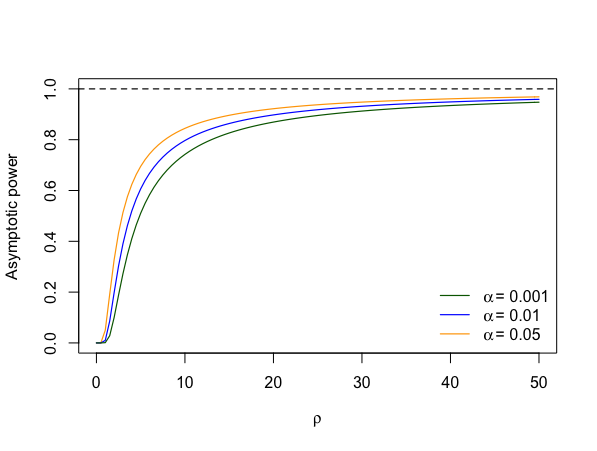
The proof of Theorem 3.1 is in Section A.3. Part 1 shows that single SPCs (i) are asymptotically frequentist and (ii) have asymptotic power less than one when $\nu_{\circ}=\nu(\theta_{\star})$. The latter behavior is illustrated in Fig. 1. On the other hand, Parts 2 and 3 show that single SPCs have asymptotic power one when $\nu_{\circ}\neq\nu(\theta_{\star})$. Thus, when the model is able to exactly capture the asymptotic mean of the statistic, the single SPC may have poor power unless $\rho$ is large – which occurs when $J_{\star}^{-1}\Sigma_{\star}J_{\star}^{-1}\gg J_{\star}^{-1}$ or $\sigma_{\circ}\gg\sigma(\theta_{\star})$. We can think of the case where the model can match the mean of the statistic as indicating “mild-to-moderate” misspecification, with the exact degree quantified by $\rho$, while the case where the model cannot match the mean of the statistic as indicating “major” misspecification. Hence, Theorem 3.1 indicates single SPCs will be effective at detecting moderate-to-major misspecification but less effective if the misspecification is mild. Depending on the application, the fact that single SPC $p$-values are nearly uniform when there are small deviations between the assumed model and data-generating process may viewed as a benefit since small deviations are almost inevitable.

Figure 1: The asymptotic power of the single 0.9-SPC against $\rho$ using a two-sided $p$-value with fixed $\alpha\in\{0.001,0.01,0.05\}$. The horizontal dashed line indicates power 1.

Example 3.2.

Consider Gaussian location model with known variance, so the parameter of interest is the mean $\theta$:

$$X_{i} \overset{\textrm{\tiny{i.i.d.}}}{\sim}\mathcal{N}(\theta,\sigma^{2}), \theta \sim\mathcal{N}(\mu,\tau^{2}).$$ (6)

Assume the data-generating distribution is $P_{\circ}=\mathcal{N}(\theta_{\circ},\sigma_{\circ}^{2})$, so the model is misspecified if $\sigma\neq\sigma_{\circ}$. For the mean statistic $T_{N}(\mathbf{X}_{N})=\overline{X}:=\frac{1}{N}\sum_{i=1}^{N}X_{i}$, if follows from Theorem 3.1 that, since $\nu_{\circ}=\nu(\theta_{\star})=\theta_{\star}$, the asymptotic power of the two-sided single $q$-SPC converges to $2\Phi(z_{\frac{\alpha}{2}}/\rho)$ with $\rho=\sigma_{\circ}/\sigma$. Thus, the single $q$-SPC can detect misspecification when the assumed data variance $\sigma^{2}$ is too small. However, when $\sigma^{2}$ is larger than $\sigma_{\circ}^{2}$, the single $q$-SPC test will have power near zero no matter how large $\sigma^{2}$ is.

Remark 3.3 (Extension to realized discrepancies).

While our focus is on the case of statistics depending only on the data, our approach and results can be extended to the case of a realized discrepancies, where the statistic depends on the data and the parameter. For example, in Section A.4 we show that, for the Gaussian location model and mean-square error statistic $T(\mathbf{X},\theta)=\frac{1}{N}\sum_{i=1}^{N}(X_{i}-\theta)^{2}$, $\mathbb{P}[p_{\text{SPC}}(\mathbf{X})<\alpha]\overset{P}{\to}\Phi(z_{\alpha}/\rho),$ where $\rho=\sigma_{\circ}^{2}/\sigma^{2}$. Hence, we reach similar conclusions about the $q$-SPC $p$-values for realized discrepancies being asymptotically well-calibrated but possibly having asymptotic power less than one.

3.2 Divided SPCs

In light of the possible poor power of the single SPC, we aim to develop an alternative split predictive check that is guaranteed to have asymptotic power of one when the model is misspecified. We build upon the single SPC by observing that, when the model is misspecified, we still expect the asymptotic distribution of the single SPC $p$-values to be non-uniform. Hence, if we have many such $p$-values, we can instead test for their uniformity. More precisely, given data $\mathbf{X}$, divide the original data into $k$ equal folds of size $N_{k}\approx N/k$. Denoting these folds by $\mathbf{X}^{(1)},\ldots,\mathbf{X}^{(k)}$, the next step is to compute the single $q$-SPC $p$-value $u_{kj}:=p_{\text{SPC}}(\mathbf{X}^{(j)})$ for each fold $j=1,\ldots,k$. To assimilate all the $k$ single SPC $p$-values, we use the Kolmogorov–Smirnov (KS) test for uniformity Massey (1951). Specifically, we define the divided SPC $p$-value as

$$p_{\text{dSPC}}(\mathbf{X}_{\text{obs}}):=p_{\text{KS}}(u_{k1},\ldots,u_{kk}),$$ (7)

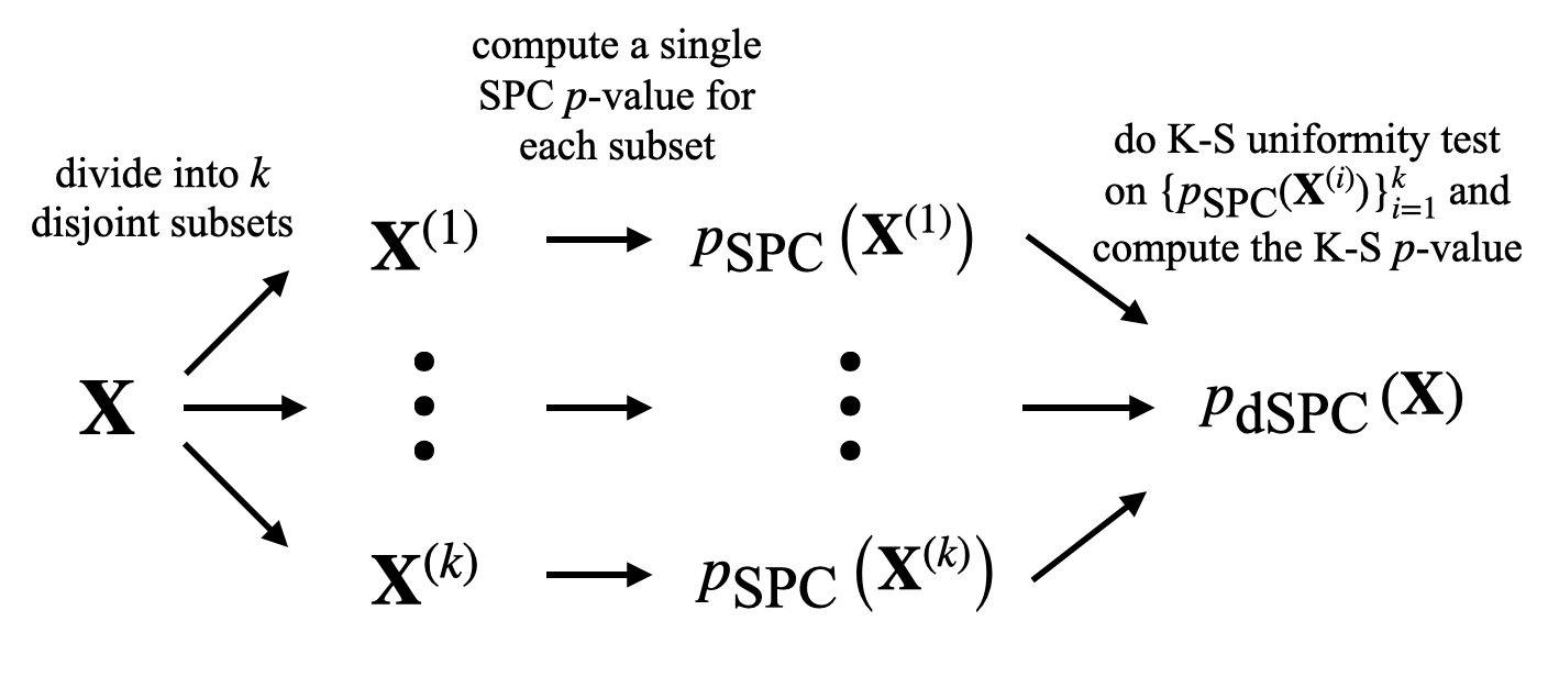
where $p_{\text{KS}}(\cdot)$ denotes the $p$-value of KS uniformity test. A schematic diagram of obtaining a divided SPC $p$-value is presented in Fig. 2.

The choice of the KS test is reasonable in light of our next result, which establishes that, when the model is correctly specified, we can bound the Kolmogorov distance between the distribution of the single SPC $p$-values and the uniform distribution. We recall that for distributions $\mu$ and $\omega$ on $\mathbb{R}$, the Kolmogorov distance is given by $d_{K}(\mu,\omega):=\sup_{u\in\mathbb{R}}|\mu((-\infty,u])-\omega((-\infty,u])|.$ We sometimes slightly abuse notation and write the distance $d_{K}(U,V)$ instead of $d_{K}(\mu,\omega)$ for random variables $U$ and $V$ having distributions $\mu$ and $\omega$. In addition to Assumption A1, the assumptions required are essentially quantitative versions of Assumptions A2 and A3. For example, we require high-probability convergence of the maximum likelihood estimator $\hat{\theta}(\mathbf{X}):=\operatornamewithlimits{arg\,max}_{\theta\in\Theta}p_{\theta}(\mathbf{X})$ and asymptotic normality of the posterior. For a set $S\subseteq\mathbb{R}^{d}$, define the constrained total variation distance $d_{TV,S}(\mu,\omega):=\sup_{B\subseteq\mathcal{B}(S)}|\mu(B)-\omega(B)|,$ where $\mathcal{B}(S)$ is the collection of all Borel subsets of $S$.

Assumption A4.

There exists a constant $s\geq 2$ such that, for any compact set $\mathcal{K}$ satisfying $\theta_{\star}\in\operatorname{Int}({\mathcal{K}})$, there exist constants $c_{\mathcal{K}},c^{\prime}_{\mathcal{K}}>0$ such that

1. $\mathbb{P}\left[\|\hat{\theta}(\mathbf{X}_{N})-\theta_{\star}\|>c_{\mathcal{K}}N^{-1/2}\right]=O(N^{-s/2})$ and

2. $\mathbb{P}\left[d_{TV,\mathcal{K}}(\Pi(\cdot\mid\mathbf{X}_{N}),\mathcal{N}(\hat{\theta}(\mathbf{X}_{N}),\Sigma_{\star}/N))>c^{\prime}_{\mathcal{K}}N^{-1/2}\right]=O(N^{-s/2})$.

Assumptions (A4-a) and (A4-b) hold under the regularity conditions listed in Hipp and Michel (1976, Section 4). These conditions essentially impose some restrictions on the smoothness of the model density and the existence of lower-order moments of the log-likelihood, as characterized by the regularity parameter $s\geq 2$. We postpone the statement and discussion of the other conditions (Assumptions A6 and A7) to Section A.3.

Theorem 3.4.

Suppose $P_{\circ}=P_{\theta_{\star}}$. If Assumptions A1, A6, A4 and A7 hold, then there exists an absolute constant $C>0$ such that

$$d_{K}\big{(}p_{\text{SPC}}(\mathbf{X}),U\big{)}<C\log^{\frac{s}{1+s}}N/N^{\frac{s}{2(1+s)}}.$$ (8)

The proof of Theorem 3.4 is in Section A.3. The guarantee holds for any choice of split proportion $q$, although the constant $C$ may depend on $q$. Hence, in the well-specified case, the KS $p$-value for these SPC $p$-values (i.e., divided SPC $p$-values) should be asymptotically uniform as long as $k\to\infty$ as $N\to\infty$. On the other hand, if the model is misspecified, the single SPC $p$-values of the subsets are not uniform asymptotically, so the KS test (and hence the divided SPC test) will have asymptotic power 1.

Figure 2: A schematic diagram of divided SPC. Divided SPC splits the original dataset into $k$ disjoint subsets $\mathbf{X}^{(i)},i=1,\ldots,k$ and computes a single SPC $p$-value for each subset. The divided SPC $p$-value is the $p$-value from the Kolmogorov-Smirnov test on all single SPC $p$-values.

3.3 Calibration and power of divided SPCs

While the arguments in favor of the divided SPC are suggestive, we need to be careful with the choice of the number of divided splits $k$ to ensure the desired asymptotic properties hold. We first investigate the calibration properties of the divided SPC when the conclusion of Theorem 3.4 holds. Let ${\sf{Unif}}$ denote the uniform distribution on $[0,1]$, $\mathbb{P}_{k}$ be the distribution of $k$ single SPC $p$-values on $N_{k}$ data and $\hat{\mathbb{P}}_{k}$ denote the corresponding empirical distribution.

Assumption A5.

There exist constants $C>0$ and $\bar{\gamma}\in(0,1]$ such that for all $\gamma<\bar{\gamma}$, $d_{K}\big{(}\mathbb{P}_{k},{\sf{Unif}}\big{)}<CN_{k}^{-\gamma/2}$.

Under the hypotheses of Theorem 3.4, Assumption A5 holds with $\bar{\gamma}=s/(s+1)$. For sufficiently regular models, any $s\geq 2$ may be chosen, in which case $\bar{\gamma}$ can be arbitrarily close to $1$.

Theorem 3.5.

If Assumption A5 holds and $k=\lfloor bN^{\beta}\rfloor$, for $b>0$ and $0<\beta<\frac{\bar{\gamma}}{\bar{\gamma}+1}$, then for any $t>0$,

$$\lim_{N\to\infty}\left|\mathbb{P}\left[k^{1/2}d_{K}\big{(}\hat{\mathbb{P}}_{k},{\sf{Unif}}\big{)}>t\right]-\left(1-F_{\mathrm{KS}}(t)\right)\right|=0,$$ (9)

where $F_{\mathrm{KS}}(\cdot)$ is the CDF of the Kolmogorov distribution. Hence, $\lim_{N\to\infty}d_{K}(p_{\text{dSPC}}(\mathbf{X}_{\text{obs}}),{\sf{Unif}})=0$.

Theorem 3.5, the proof of which is in Section A.5, suggests that $k$ cannot grow too fast compared to $N$ if we wish to control the test size. If $s$ can be chosen arbitrarily large, then we may take $k=O(N^{\beta})$ for any $\beta\in(0,1/2)$. On the other hand, if we only assume $s\geq 2$, then we must take $\beta\in(0,2/5)$.

Having established the correct calibration of divided SPC $p$-values, we next show that when the model is misspecified the asymptotic power of divided SPC is one.

Theorem 3.6.

If $\liminf_{k\rightarrow\infty}d_{K}(\mathbb{P}_{k},{\sf{Unif}})>0$, then for any $t>0$,

$$\lim\limits_{k\rightarrow\infty}\mathbb{P}\left[\mathchoice{{\hbox{$\displaystyle\sqrt{k\,}$}\lower 0.4pt\hbox{\vrule height=6.94444pt,depth=-5.55559pt}}}{{\hbox{$\textstyle\sqrt{k\,}$}\lower 0.4pt\hbox{\vrule height=6.94444pt,depth=-5.55559pt}}}{{\hbox{$\scriptstyle\sqrt{k\,}$}\lower 0.4pt\hbox{\vrule height=4.8611pt,depth=-3.8889pt}}}{{\hbox{$\scriptscriptstyle\sqrt{k\,}$}\lower 0.4pt\hbox{\vrule height=3.47221pt,depth=-2.77779pt}}}d_{K}\big{(}\hat{\mathbb{P}}_{k},{\sf{Unif}}\big{)}>t\right]=1.$$ (10)

The proof of Theorem 3.6 is in Section A.5. We note that when the model is misspecified and $\rho\neq 1$, Theorem 3.5 shows that the distribution of SPC $p$-values is nonuniform, so the hypotheses of Theorem 3.6 hold.

4 Using Split Predictive Checks in Practice

We next provide some guidance on how to apply split predictive checks in practice, which we verify in our simulation studies in Section 5.

4.1 Using single SPCs

As discussed earlier, most of the assumptions required by Theorem 3.1 are quite mild. The only assumption that the analyst has to be careful with is Assumption A2, which requires the choice of test statistic to be asymptotically normal.

Choosing $q$

The split proportion $q$ controls the relative weight placed on two forms of misspecification quantified by $\rho$: the uncertainty of the statistic $T$ and the optimal parameter $\theta_{\star}$. Choosing $q$ large assigns more weight to the comparison between $\sigma_{\circ}$ and $\sigma(\theta_{\star})$ while a small $q$ emphasizes the mismatch between frequentist sampling-based uncertainty $J_{\star}^{-1}\Sigma_{\star}J_{\star}^{-1}$ and standard posterior uncertainty $J_{\star}^{-1}$ in the direction $\dot{\nu}(\theta_{\star})$. A canonical choice for $q$ is 0.5, which treats the well-calibration of the two types uncertainty as equally important.

In a small-sample regime, extreme values for $q$ are not recommended. Small split proportions $q$ may result in an inadequate amount of observed data, while choosing $q$ large may result in poor estimation of the statistic. Hence, we recommend choosing a moderate value for $q$ (e.g., 0.5 or 0.7) when the dataset size is fairly small relative to the model complexity.

Accounting for model structure

There are many ways to implement splitting the data for structured models such as those for time-series or spatial data. The analyst must then take into account what aspects of the data the test statistic captures in order to choose an effective splitting strategy. We discuss two canonical cases: hierarchical and time-series models.

We first consider the case of a two-level hierarchical structure:

$$\begin{split}\eta_{0}&\sim H\\ \eta_{i}&\overset{\textrm{\tiny{i.i.d.}}}{\sim}G_{\eta_{0}}\quad(i=1,\ldots,I),\\ X_{ij}&\overset{\textrm{\tiny{indep}}}{\sim}F_{\eta_{i}}\quad(i=1,\dots,I;j=1,\dots,J_{i}).\end{split}$$

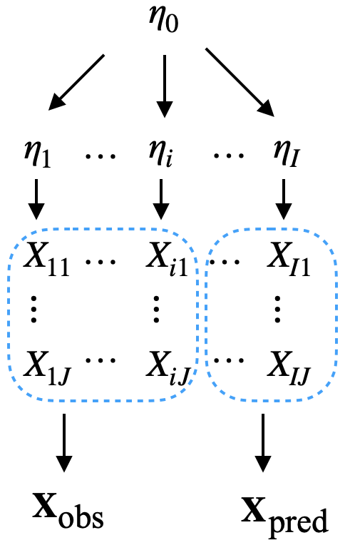
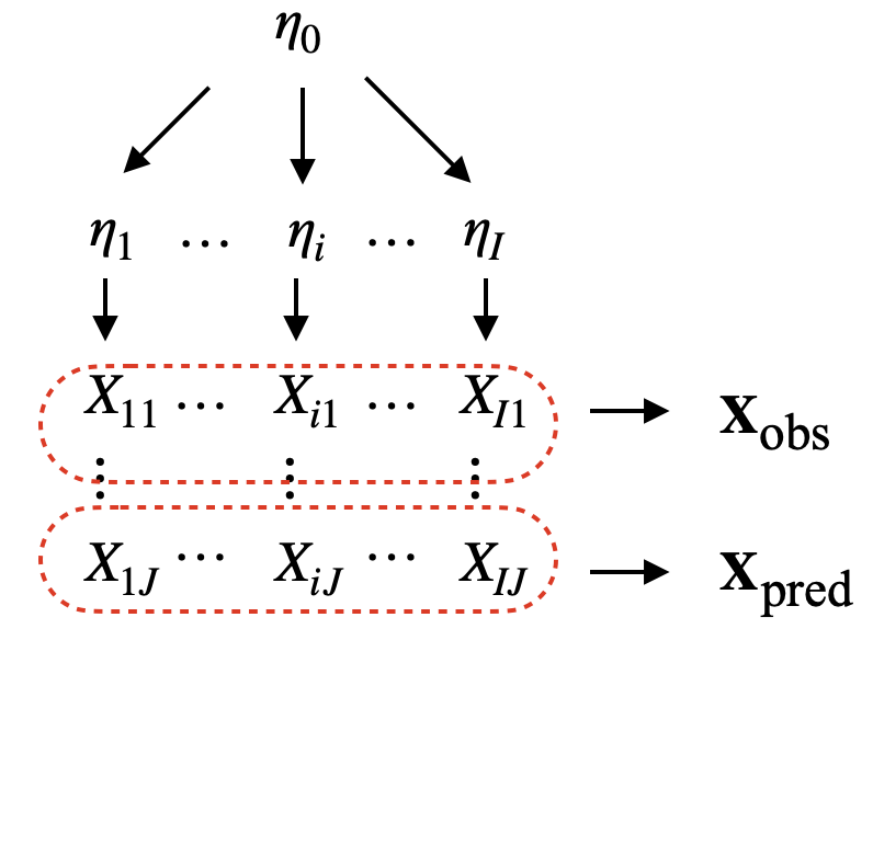
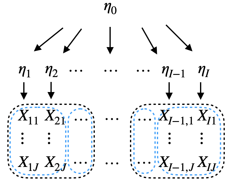
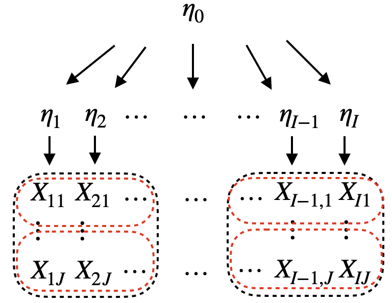
When applying the single SPC to such a model, we have two ways to split the data: either across or within the groups, as shown in Fig. 3. We call the former single cross-SPC and the latter single within-SPC. Which split is preferred depends on which level of misspecification is of interest. For instance, if the analyst is interested in misspecification at the observation-level (that is, in the $F_{\eta_{i}}$) and has chosen an appropriate test statistic, then the single within-SPC would be appropriate since it will compare data from each group with the predictive distribution for that group. On the other hand, if the analyst is interested in group-level misspecification (that is, in $G_{\eta_{0}}$), then the single cross-SPC will compare data across different groups. Similar considerations could be applied to more complex hierarchical structures.

(a) single cross-SPC

(b) single within-SPC

Figure 3: A schematic diagram of single cross-SPC (left) and single within-SPC (right) for a two-level hierarchical model.

For a time-series model, there are two splitting strategies to do the single split. In the extrapolated single SPC, take the first $q$ proportion of data as the observed data $\mathbf{X}_{\text{obs}}$ and hold out the rest. In the interpolated single SPC, for every $m\ll N$ observations, take the first $qm$ as observed data and the reminder as held out. The extrapolated single SPC can be views as the “extreme” interpolated single SPC with $m=N$. But assuming $m\ll N$, in the case of the interpolated SPC, both $\mathbf{X}_{\text{obs}}$ and $\mathbf{X}_{\text{ho}}$ contain information along the whole time-series. Which choice is appropriate will depend on how the analyst is using the model. For short-term prediction or analysis of a fixed dataset, interpolation may be appropriate, while for medium-to-long-term prediction extrapolation might be a better choice.

4.2 Using divided SPCs

In addition to $q$, divided SPCs require choosing the number of splits $k$, while structured models also require additional considerations. We address each in turn.

(a) cross-divided cross-SPC

(b) cross-divided within-SPC

(c) within-divided cross-SPC

(d) within-divided within-SPC

Figure 4: An explanatory diagram of cross-divided cross-SPC (top left), cross-divided within-SPC (top right), within-divided cross-SPC (bottom left) and within-divided within-SPC (bottom right) for a hierarchical model. We use black dotted circles to denote the $k$ disjoint subsets in divided SPCs. Blue dotted circles refer to a single cross-SPC test for the subset. Red dotted lines indicate a single within-SPC $p$-value for each subset.

Choosing $q$ and $k$

The choice of $q$ requires the same considerations as in the single SPC case. However, now we must judge the dataset size by $N_{k}$, the sample size used to compute the $k$ single $q$-SPC $p$-values. The performance of divided SPCs could be significantly affected by the number of splits $k$. In general, a larger $k$ will improve the power of the KS test but lead to $N_{k}$ being smaller, which may result in single $q$-SPC $p$-values being closer to uniform. We suggest using divided SPCs when $N$ is very large, so choosing $k=\lfloor N^{\beta}\rfloor$ with $\beta$ as large as possible is appropriate. Hence, based on Theorem 3.5 and the discussion that follows, for sufficiently regular models we suggest taking $\beta$ just below $1/2$ (e.g., $0.49$). For less regular models, a safe choice is $\beta$ just below $2/5$ (e.g., $0.39$).

Accounting for model structure

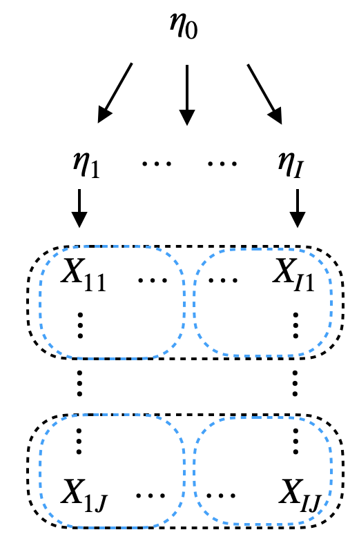
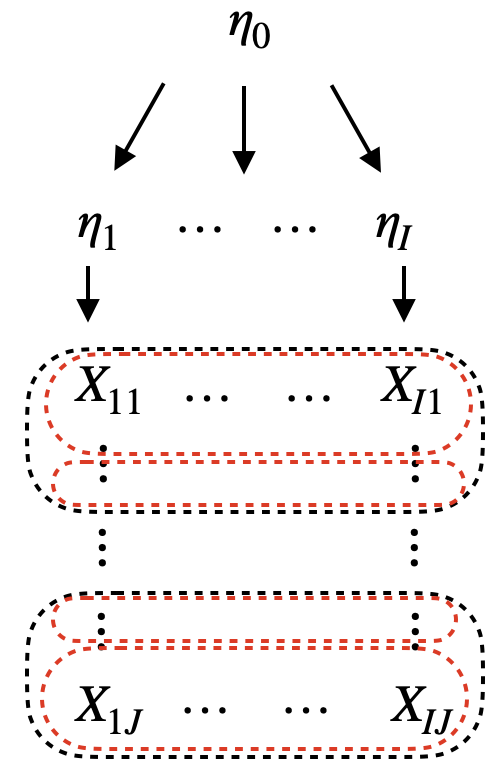
Divided SPCs have two splitting steps: first divide the original data into $k$ subsets, then apply single splits to each of the subset. For the hierarchical model Section 4.1, each split step can be across- or within-groups. Therefore, we have four possibilities, which we illustrate in Fig. 4. For $\mathsf{A},\mathsf{B}\in\{\text{cross},\text{within}\}$, we refer to using the $\mathsf{A}$ split for the first step and the $\mathsf{B}$ split for the second step as the $\mathsf{A}$-divided $\mathsf{B}$-SPC. For example, the cross-divided within-SPC refers to doing cross-group splits to get subsets and single within-SPC for each subset.

These four types of divided SPCs can effectively apply to different scenarios. Suppose a user aims to detect the lower-level misspecification. From the analysis of single SPCs in hierarchical model, one should choose from cross-SPCs. Indeed, asymptotically cross-divided cross-SPCs and within-divided cross-SPC produce similar results. However, when the data size is small, we suggest choosing within-divided cross-SPC, which provides more lower-level information for each dataset compared to doing cross-group splitting twice. On the other hand, if the user is interested in finding mismatches in the group level, then with large dataset, both cross-divided within-SPCs and within-divided within-SPC should work well. We expect that for small data sets cross-divided within-SPC will usually be preferred.

The application of divided SPCs to time-series data works in a similar way as in hierarchical model. For each level of splitting in divided SPCs, we have two choices: extrapolation and interpolation. Interpolated splitting allows each subset to contain data across the whole time-series from the original dataset while extrapolated splits only include partial information for each subset. Depending on the purpose of the study, the user can choose different ways of splitting with SPCs.

4.3 Comparison of SPCs to posterior predictive checks

Posterior predictive checks (PPCs) and the two types of SPCs offer complimentary strengths in terms of power performance, computational efficiency, and applicability to small or large datasets.

Power

To discuss the power of the three checks, we roughly categorize misspecification into three types: “major” (when $\nu_{\circ}$ and $\nu(\theta_{\star})$ are very different), “moderate” (when $\nu_{\circ}$ and $\nu(\theta_{\star})$ are equal or nearly equal but $\sigma_{\circ}/\sigma(\theta_{\star})$ is large) and “subtle-to-moderate”(when $\nu_{\circ}\approx\nu(\theta_{\star})$ and $\sigma_{\circ}/\sigma(\theta_{\star})$ is not very large). Single SPC works well when the misspecification is moderate or major, as shown in Theorem 3.1. However, for subtle-to-moderate misspecification the asymptotic power of single SPC can be small. Divided SPC, on the other hand, is effective in case of subtle-to-moderate misspecification, as demonstrated by Theorem 3.6. PPCs only has good power only when there is major misspecification, as otherwise double use of the data leads to conservative $p$-values (Robins, van der Vaart and Ventura, 2000).

Dataset size and computational efficiency

All three methods require similar computational effort. PPCs use only the already estimated posterior. Single SPCs require estimating the posterior of the observed split of the data, which will typically require about half the computational effort of the original posterior estimate since we recommend choosing $q\approx 0.5$. While divided SPCs require one posterior computation for each subset, the dataset sizes are small so the total cost should be roughly equal to that of estimating the original posterior. As for different dataset sizes, divided SPCs requires a moderate-to-large dataset since when the data is small, there is insufficient amount of data in each subset of size $N_{k}$. On the other hand, both PPC and single SPC remain effective in the small data regime.

5 Simulation Studies

To validate our theory from Section 3 and guidelines from Section 4, and investigate the finite-sample effects of SPC tuning parameters (the split proportion $q$ and, for the divided SPC, the number of folds $k$), we carry out two simulation studies, with a conjugate Poisson model and a Gaussian hierarchical model. We compare SPCs to other general-purpose predictive checks: the widely used posterior predictive check (PPC) and the first version of population predictive check (POP-PC-v1) since, like SPCs, it avoids double use of the data.

5.1 Poisson model

We consider the conjugate Poisson model $P_{\theta}={\sf{Poiss}}(\theta)$, a Poisson distribution with rate parameter $\theta$, and prior $\Pi_{0}={\sf{Gamma}}(0.1,0.2)$, a gamma distribution parameterized by the shape and rate. We investigate the behavior of the predictive checks for two data-generating distributions, the well-specified model $P_{\circ}={\sf{Poiss}}(2)$ and the misspecified model $P_{\circ}={\sf{NegBin}}(2,0.01)$, a negative binomial distribution parameterized by the mean and dispersion. We implement all methods using four statistics: (i) empirical mean $T_{N}(\mathbf{x})=\frac{1}{N}\sum_{i=1}^{N}x_{i}$, (ii) 2nd moment $T_{N}(\mathbf{x})=\frac{1}{N}\sum_{i=1}^{N}x_{i}^{2}$, (iii) 3rd moment $T_{N}(\mathbf{x})=\frac{1}{N}\sum_{i=1}^{N}x_{i}^{3}$ and (iv) mean squared error (MSE) $T_{N}(\mathbf{x},\theta)=\frac{1}{N}\sum_{i=1}^{N}(x_{i}-\mathbb{E}[\mathbf{X}_{i}\mid\theta])^{2}$. Similar results are also obtained in the case of the Gaussian location model, which we present in Section B.2.1.

Single SPCs

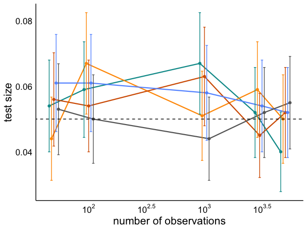
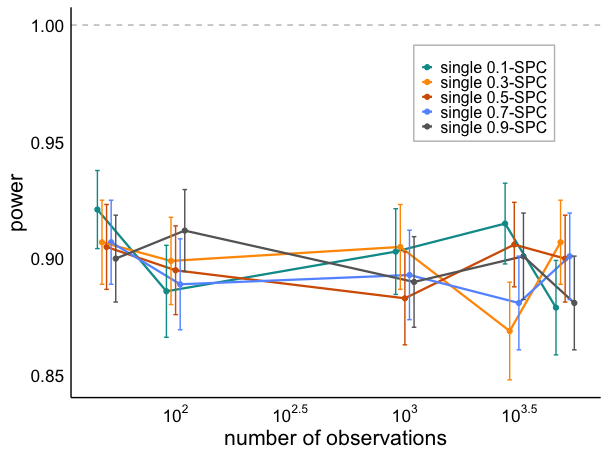
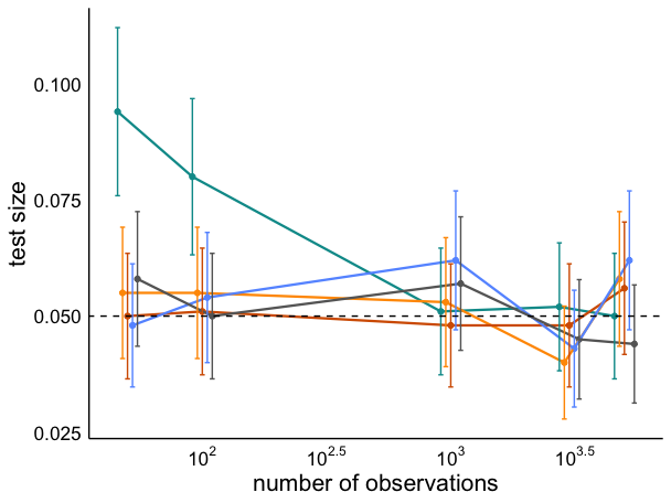
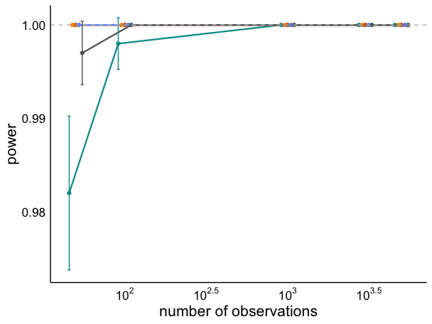
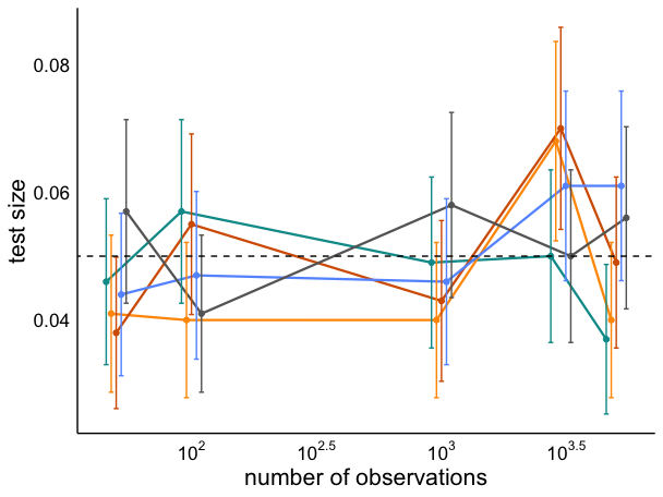
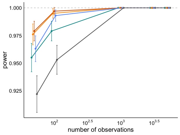
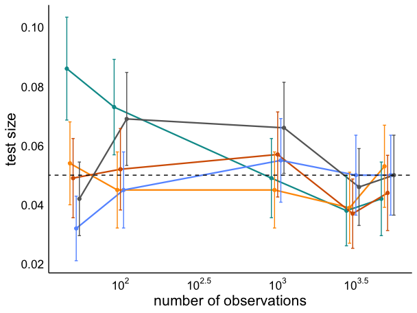
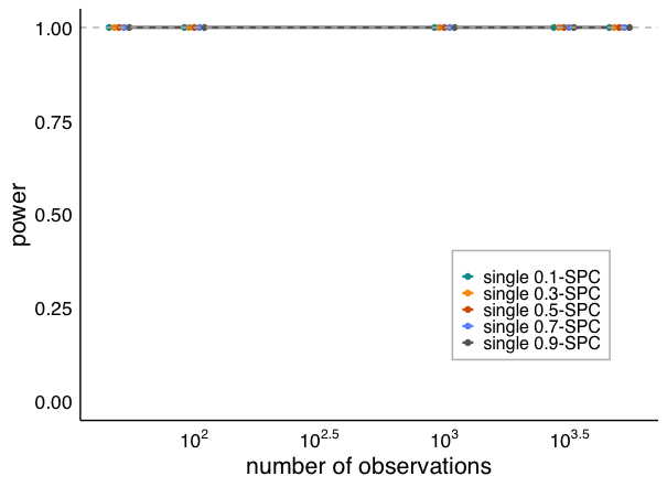
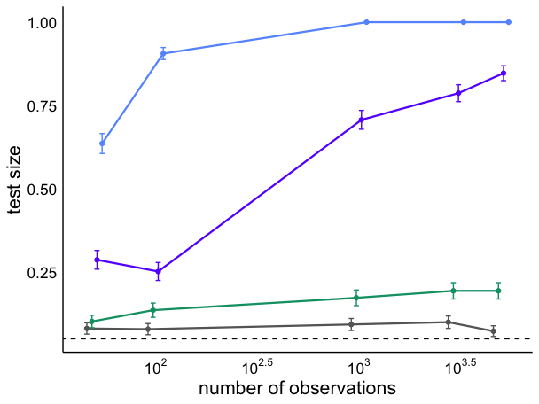
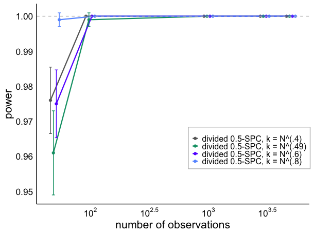
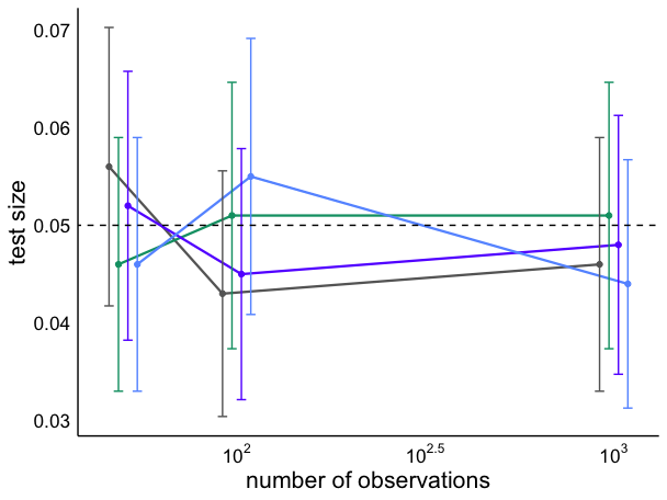
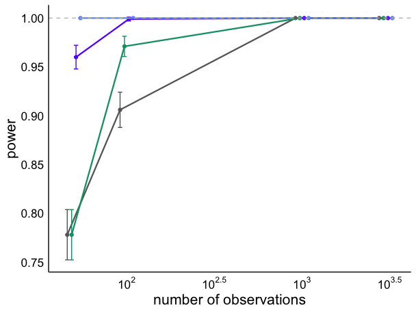
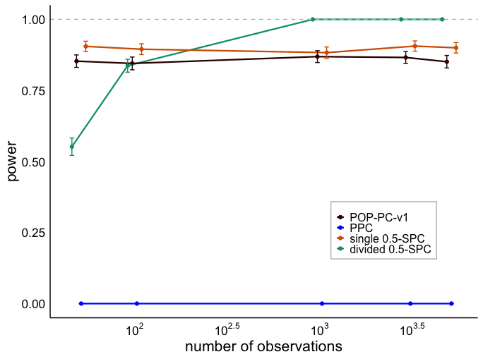
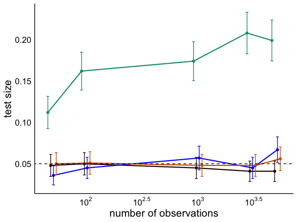
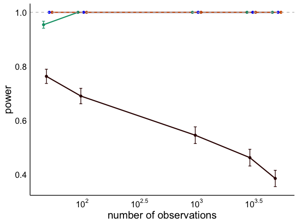
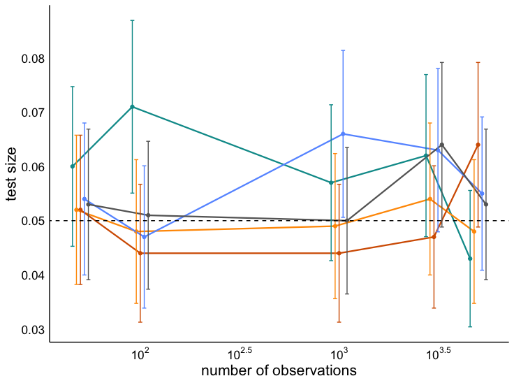
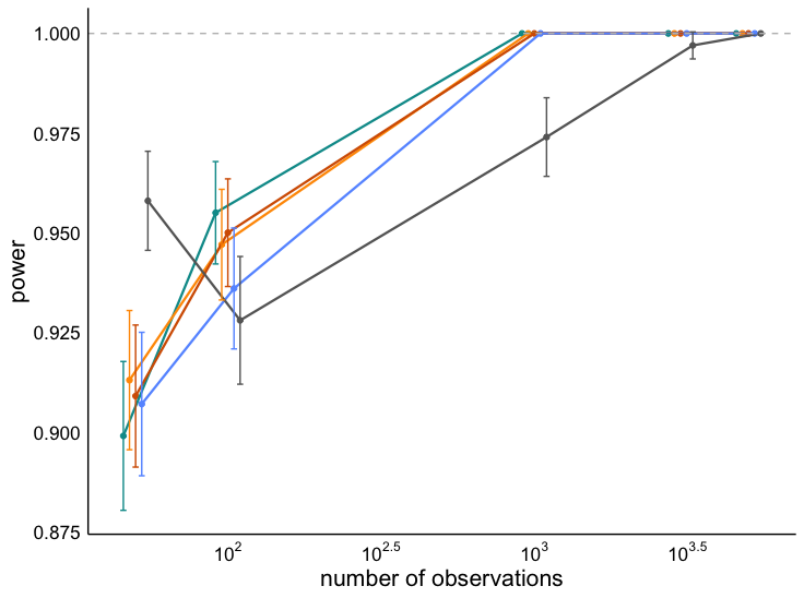
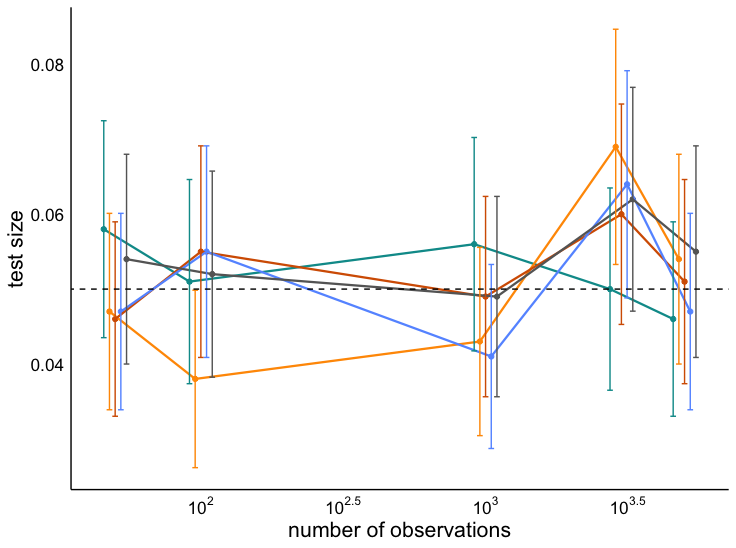
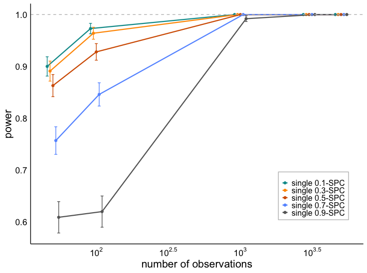
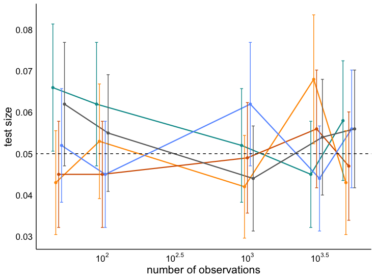
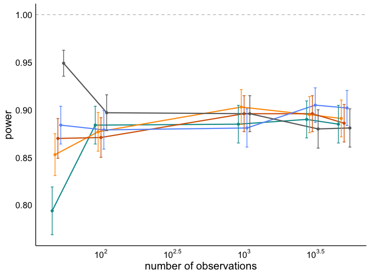
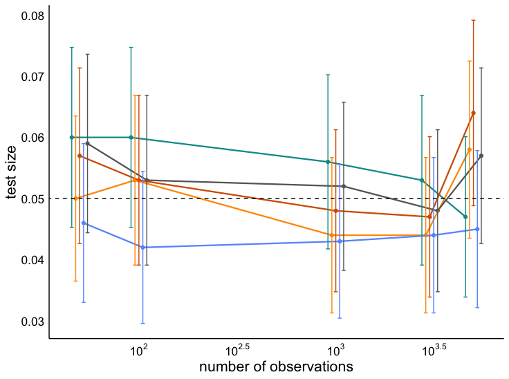
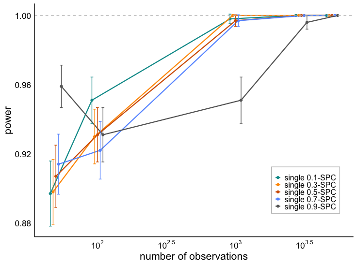
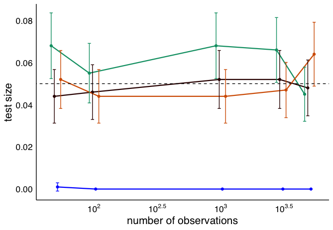
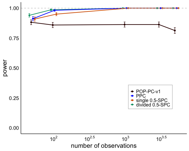
Figure 5 confirms that, as predicted by Theorem 3.1, the test size is well controlled. The choice of $q$ controls the asymptotic behavior of single SPCs when $\nu_{\circ}=\nu(\theta_{\star})$ and has no impact when $\nu_{\circ}\neq\nu(\theta_{\star})$. For the small sample size regime, a moderate split proportion such as $q=0.5$ is preferable to an extreme one. As shown in Figs. 5a and 5d, the single SPC with $q=0.1$ has a slightly larger Type I error compared to other proportions when $N=50$, while single SPC with $q=0.9$ produces the smallest power when $N=1000$. Figure 5b empirically verifies the limitations of single SPCs documented in Theorem 3.1: for all single SPCs using the mean statistic and where subtle-to-moderate misspecification occurs, the power stays around 0.9 and has no tendency to increase as the sample size grows. We present results for 3rd moment and MSE statistics in Fig. B.21, which correspond to moderate misspecification case and thus single SPC achieves power 1 asymptotically .

(a) mean

(b) mean

(c) 2nd moment

(d) 2nd moment

Figure 5: Test size and power plots for single SPC with different split proportions $q\in\{0.1,0.3,0.5,0.7,0.9\}$, under conjugate Poisson model. The vertical bars represent the $95\%$ confidence intervals for the test size or power estimates. Each test size and power are estimated with $1000$ single SPC $p$-values that are computed with $1000$ datasets of size $N\in\{50,100,1000,3000,5000\}$. The dashed horizontal line in the test size plots indicates the significance level $\alpha=0.05$ and the dashed line in the power plots is at 1.

Divided SPCs

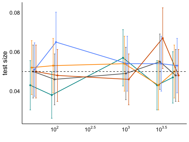
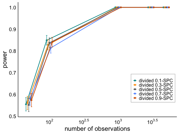
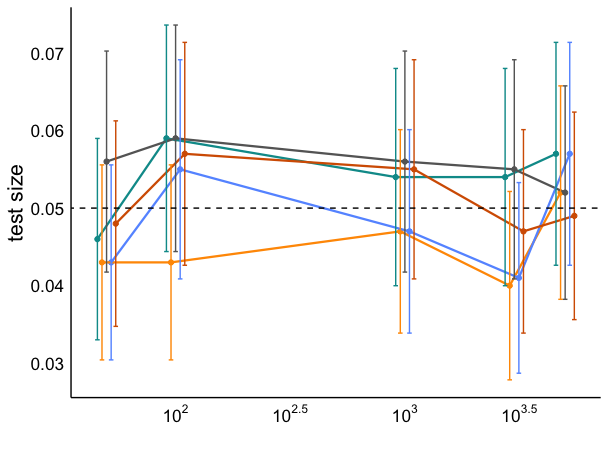
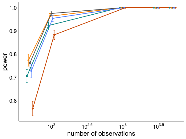
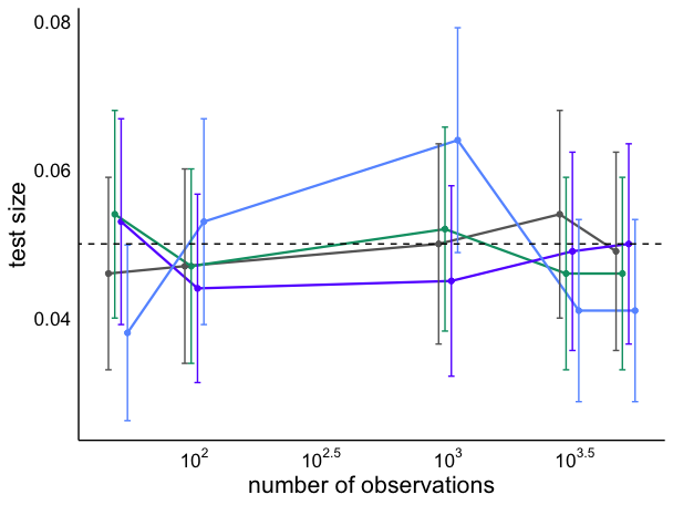
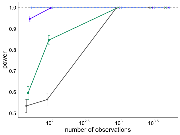
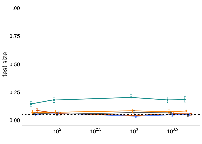
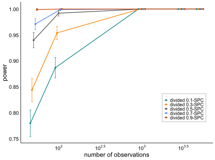
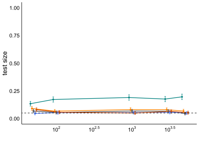
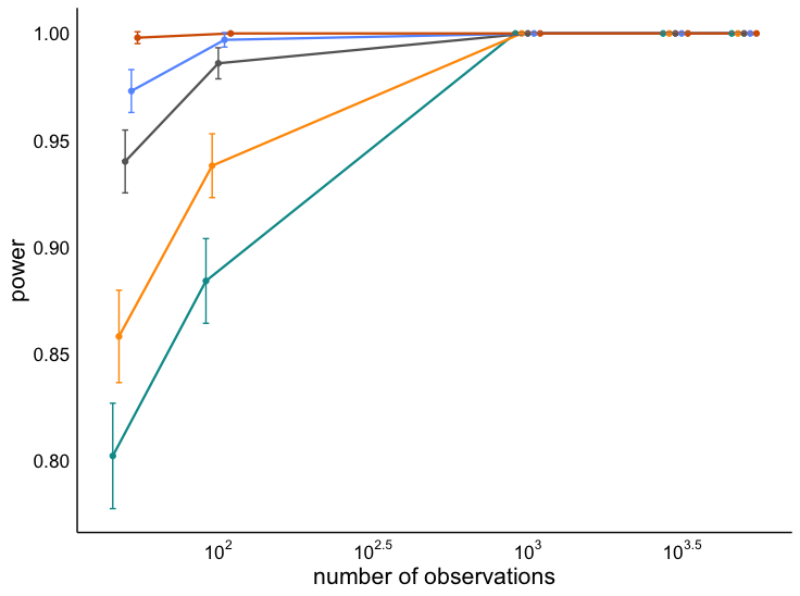
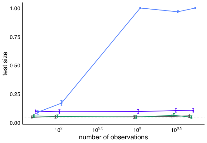
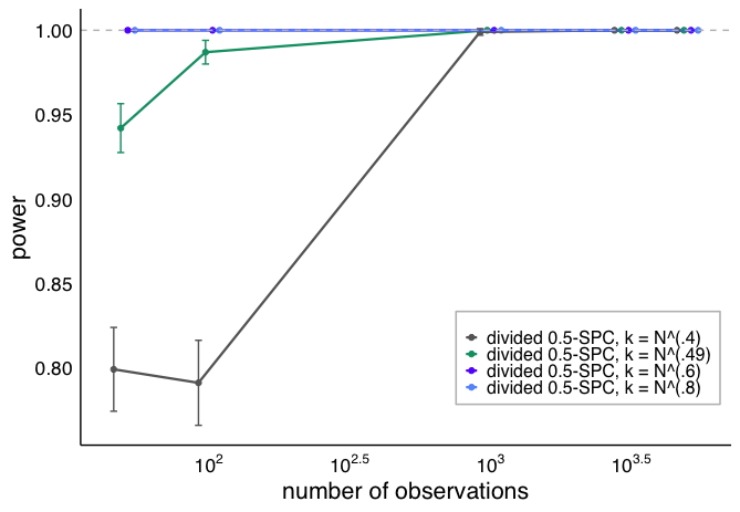
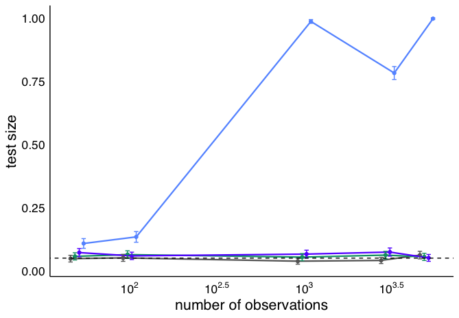
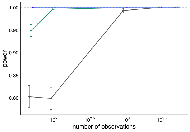
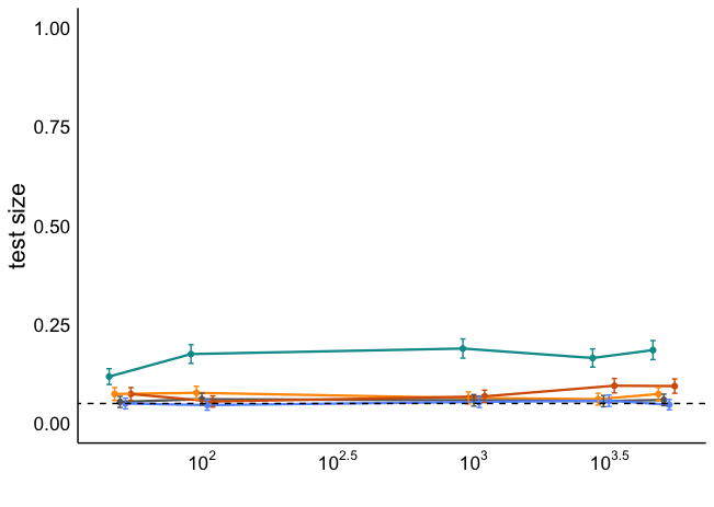
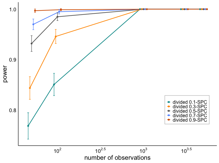
We now switch our attention to divided SPCs. Initially we fix $k=N^{0.49}$ and vary $q$. Fig. 6b shows that the divided SPC has asymptotic power 1 and since $\rho=\sigma_{\circ}/\sigma(\theta_{\star})$, the split proportion makes no difference in the power performance of divided SPC given a large sample size. However, when dealing with a sample of small or moderate sizes, one needs to be careful with the choice of split proportion for divided SPC. As shown in Fig. 6a, the divided SPC with both $q=0.1$ and $q=0.9$ fail to control the test size well even when $N=5000$. Therefore, even though the power increases with $q$, in the small-to-moderate sample-size regime the best choice for the proportion is $q=0.5$. Similar results for 2nd and 3rd moments are presented in Fig. B.22.

Effect of number of folds $k$

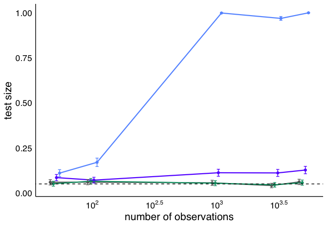
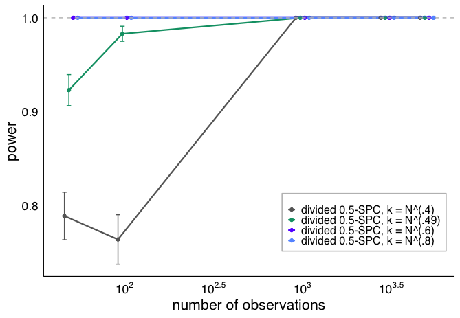
To investigate the effect of different scalings of $k$, we fix the split proportion $q=0.5$ and consider $k=N^{\beta}$ for different choices of $\beta$. Fig. 6c shows that with $\beta>1/2$, the test size is not well controlled, which is in agreement with conclusion of Theorem 3.5 that only guarantees the divided SPC is asymptotically well-calibrated when when $\beta\in(0,1/2)$. On the other hand, choosing small $\beta$ produces insufficient number of folds and thus degrades the power of the KS test. We find that $\beta\approx 1/2$ provides the best power while $\beta\approx 0.4$ has smaller power. Results for other statistics are presented in Fig. B.23.

(a)

(b)

(c)

(d)

Figure 6: (a) & (b): Test size and power for divided SPC with mean statistic, $k=N^{0.49}$, and varying $q\in\{0.1,0.3,0.5,0.7,0.9\}$, under the conjugate Poisson model. (c) & (d): Test size and power for divided SPC with 3rd moment statistic, $q=0.5$, and varying the number of folds $k\in\{N^{0.4},N^{0.49},N^{0.6},N^{0.8}\}$. See Fig. 5 for further explanation and experimental details.

Comparison to PPC and POP-PC-v1

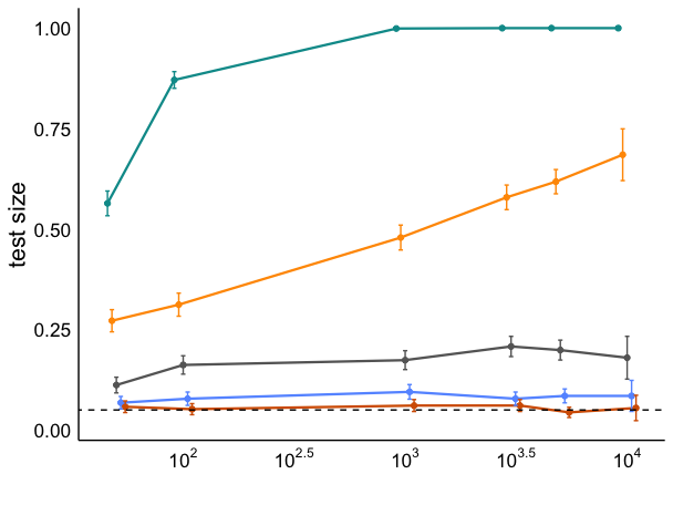
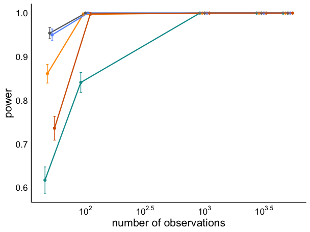
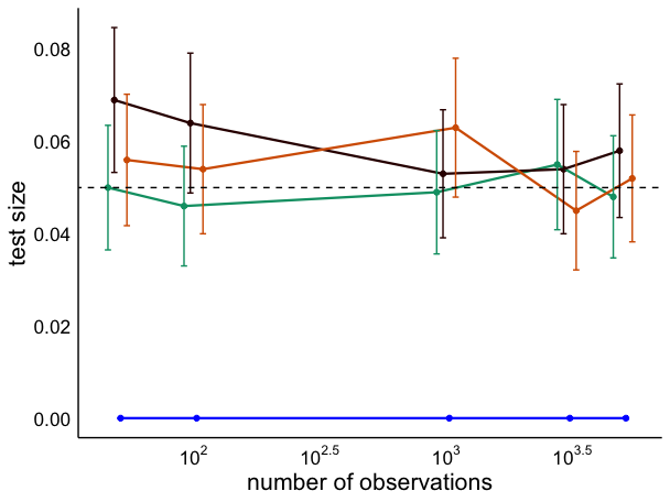
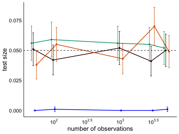
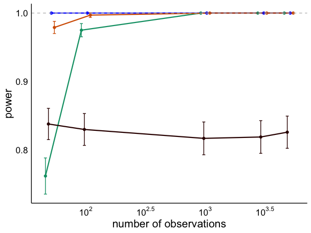
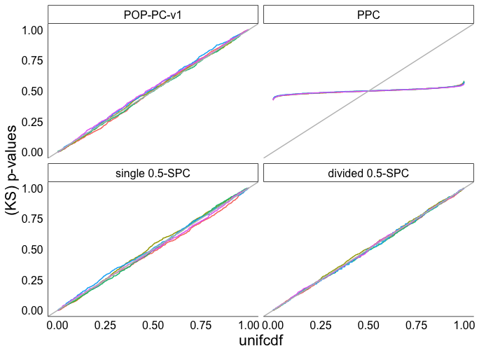
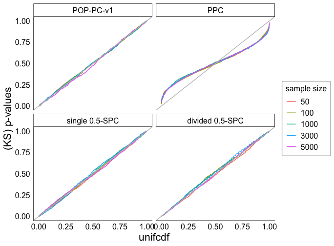
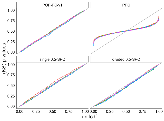
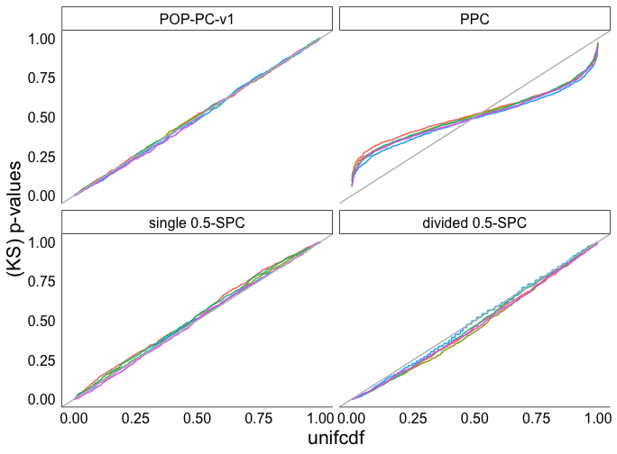
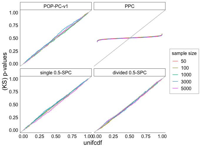
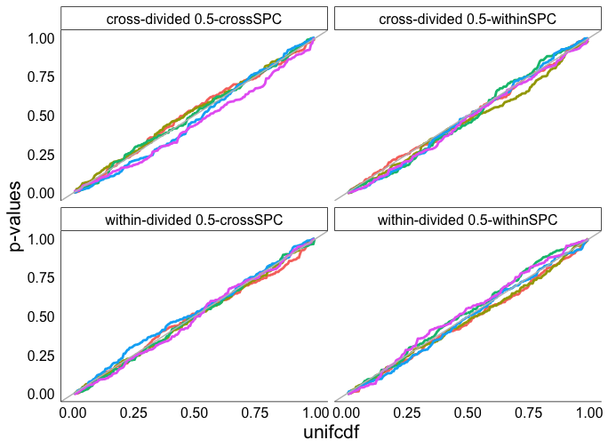
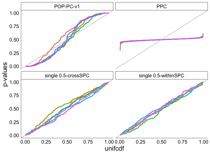
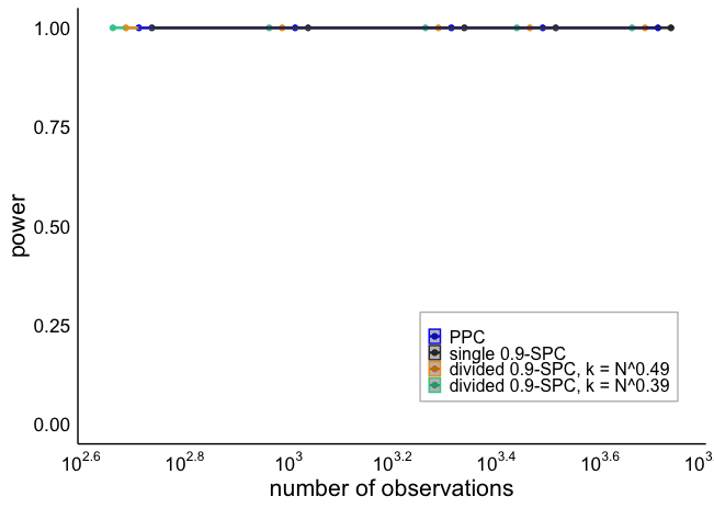
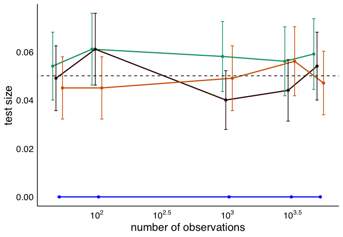
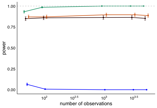
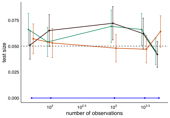
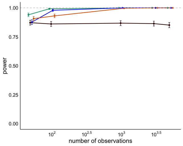
We compare the single $0.5$-SPC and divided $0.5$-SPC with $k=N^{0.49}$ to the PPC and POP-PC-v1. Figure 7b demonstrates divided SPC is very sensitive to misspecification when the sample size is large. In this case, the PPC has power near zero and the power of both the POP-PC-v1 and single 0.5-SPC stabilizes below one. Figures 7d and 7f show that for the 2nd moment and 3rd moment statistics, all methods have power approaching one, except that POP-PC-v1. Figs. 7a, 7c and 7e show that all candidate checks control the test size well. However, even with the smallest test size, PPC fails to produce frequentist $p$-values for all the three statistics, while POP-PC-v1, single SPC, and divided SPC all have $p$-values that are close to uniform under the null model (Fig. B.24).

(a) mean

(b) mean

(c) 2nd moment

(d) 2nd moment

(e) 3rd moment

(f) 3rd moment

Figure 7: Test size and power plots in log scale for different checking methods and statistics under the conjugate Poisson model. We display experiments for $N\in\{50,100,1000,3000,5000\}$. All SPCs choose proportion as $q=0.5$ and for divided SPCs, the number of splits is set as $k=N^{0.49}$.

Effect of the degree of misspecification

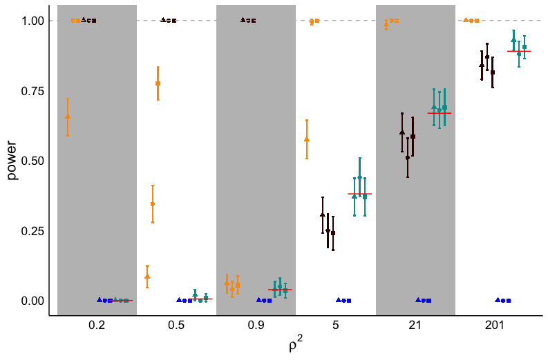
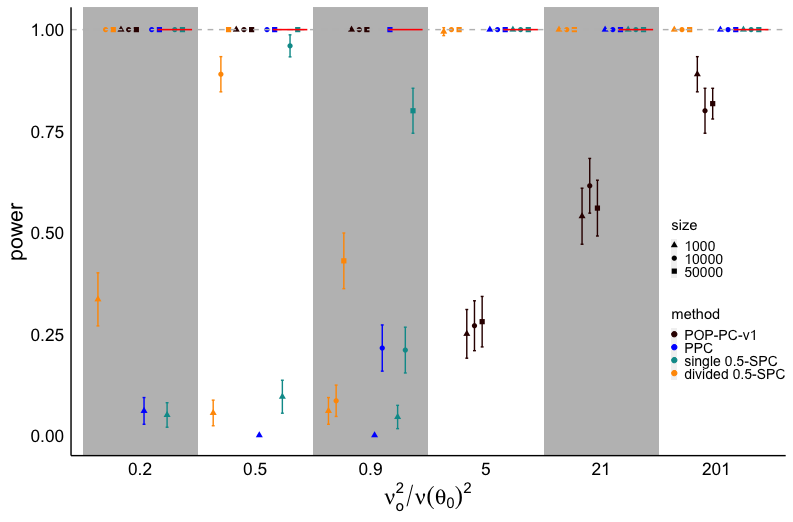
To investigate how the degree of misspecification affects each predictive check, we use the data-generating distributions $P_{\circ}={\sf{NegBin}}(2,\tau)$ and $P_{\circ}={\sf{Binom}}(30,p)$ to create over- and under-dispersed data and compare the asymptotic power of each method given different types of misspecification. Using a mean statistic in this case yields $\nu_{\circ}=\nu(\theta_{\star})$, so the degree of misspecification is effectively characterized by $\rho={\sigma_{\circ}}/{\sigma(\theta_{\star})}$ from Theorem 3.1. For the negative binomial model $\rho^{2}=1+2/\tau$ and for the binomial model $\rho^{2}=1-p$. Hence, varying $\tau\in\{0.01,0.1,0.5\}$ for the negative binomial model and $p\in\{0.1,0.5,0.8\}$ for the binomial model leads to the subtle-to-moderate misspecification scenarios $\rho^{2}\in\{0.2,0.5,0.9,5,21,201\}$. Fig. 8a shows that, as expected, the power of single SPC stabilizes near zero for $\rho^{2}<1$ but approaches one when $\rho^{2}\gg 1$. The power of divided SPC, on the other hand, reaches one for all cases except the nearly well-specified one of $\rho^{2}=0.9$. The power of PPC is zero in all cases. The power of POP-PC-v1 is inferior to single SPC when $\rho^{2}>1$ but close to one when $\rho^{2}<1$. Switching to the 2nd moment statistic, $\nu_{\circ}\neq\nu(\theta_{\star})$ so there is major misspecification. As expected, Fig. 8b shows that PPC, single and divided SPC all succeed to capture such major misspecification with power 1 given large datasets, while POP-PC-v1 has power depending on how different $\nu(\theta_{\star})$ and $\nu_{\circ}$ are when model is over-dispersed. On the whole, these results suggest that, when used together, single and divided SPC are superior to using either or both PPC and POP-PC-v1.

(a) mean

(b) $2$nd moment

Figure 8: The power plots of candidate checks given different levels of misspecification with conjugate Poisson model. The mismatch types are designed by varying the dispersion parameters $\tau\in\{0.01,0.1,0.5\}$ in ${\sf{NegBin}}(2,\tau)$ and $p\in\{0.1,0.5,0.8\}$ in ${\sf{Binom}}(30,p)$. We display experiments for all candidate methods given sample sizes $N\in\{1000,10000,50000\}$. The red solid lines indicate theoretical asymptotic power of single SPC computed from Theorem 3.1. All SPCs choose proportion as $q=0.5$ and for divided SPCs, the number of splits is set as $k=N^{0.49}$.

Effect of the prior

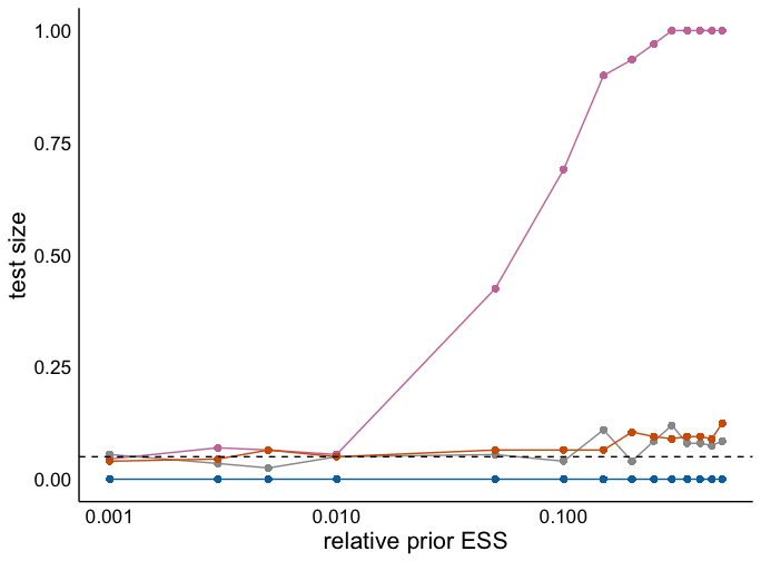
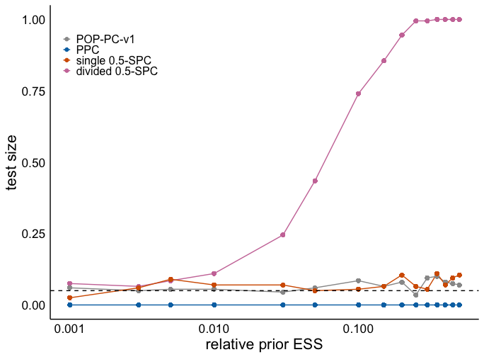
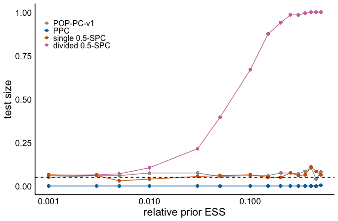
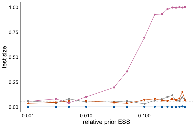
Finally, we investigate the effect of the prior on the test size of the predictive checks. Conjugate exponential families lend themselves to the definition of a prior effective sample size (ESS) (though see Reimherr, Meng and Nicolae (2021) for an extension to other models). For a Poisson model with a ${\sf{Gamma}}(\alpha,\beta)$ prior, the prior ESS is $N_{0}=\beta$. We measure the prior impact in terms of the relative prior ESS is defined as $r:=\frac{N_{0}}{N_{0}+N_{*}}$, where $N_{*}$ is the number of samples to construct a single posterior distribution. For PPC and POP-PC-v1, $N_{*}=N$ while for the SPCs $N_{*}=N_{\text{obs}}$. We set $N_{*}=50$ and $\theta_{\circ}=25$ for all methods, then vary $\beta$ so that $r$ varies between $0.001$ and $0.5$ using the formula $\beta=\frac{r}{1-r}N_{*}$. To mimic a realistic scenario, we chose $\alpha$ such that, for a given $\beta$, the true parameter $\theta_{\circ}$ lies at the $95$th quantile of the prior distribution. Figure 9 shows that for the mean and 2nd moment statistics, single SPC and POP-PC-v1 fail to control the test size when $r_{\text{adj}}\geq 0.1$ while divided SPC fails when $r_{\text{adj}}\geq 0.01$. Figure B.25 shows similar results for the case when $\theta_{\circ}=100$. Hence, we do not recommend using single SPCs when $r_{\text{adj}}\geq 0.1$ or divided SPCs when $r_{\text{adj}}\geq 0.01$.

(a) Mean

(b) 2nd moment

Figure 9: Relative prior ESS versus test size for POP-PC-v1, PPC, single $0.5$-SPC and divided $0.5$-SPC with $k=N^{0.49}$ for under the conjugate Poisson model. We set $\theta_{\star}=25$ for the data-generating distribution and adjust the prior parameters so that $\theta_{\star}$ is at the 95th quantile of the prior.

5.2 Gaussian hierarchical model

Next, we compare SPCs and the other predictive checks using the two-level Gaussian hierarchical model from Bayarri and Castellanos (2007), which corresponds to the model in Section 4.1 with $F_{\eta_{i}}=\mathcal{N}(\eta_{i},4)$, $G_{\eta_{0}}=\mathcal{N}(\mu_{0},\sigma_{0}^{2})$, and an improper prior $H$ on $\eta_{0}=(\mu_{0},\sigma^{2}_{0})$ with density $h(\mu_{0},\sigma^{2}_{0})=\sigma_{0}^{-2}$. To illustrate the use of SPCs with different types of misspecification, we simulate data from four data-generating distributions.

1. Simulate data from the assumed model,

   $$X_{ij} \mid\eta_{i}\sim\mathcal{N}(\eta_{i},4), \eta_{i} \sim\mathcal{N}(0,1).$$ (11)

2. Simulate group means from a gamma distribution,

   $$X_{ij}\mid\eta_{i} \sim\mathcal{N}(\eta_{i},4), \eta_{i} \sim{\sf{Gamma}}(0.6,0.2),$$ (12)

   which produces misspecification across groups.

3. Simulate the observations from normal distribution but with a larger variance compared to the assumed model,

   $$X_{ij}\mid\eta_{i} \sim\mathcal{N}(\eta_{i},8), \eta_{i} \sim\mathcal{N}(0,1),$$ (13)

   which produces misspecification within groups.

4. Simulate the observations from a log-normal distribution,

   $$\ln(X_{ij})\mid\eta_{i} \sim\mathcal{N}(\eta_{i},4), \eta_{i} \sim\mathcal{N}(0,1),$$ (14)

   which produces misspecification both across and within groups.

Statistics for hierarchical model

Let $Q(\mathbf{x})$ denote the $75$th quantile of data $\mathbf{x}$ and $\bar{x}_{i}$ be the mean of the $i$th group of observations. We employ three statistics in our simulations: (i) the grand mean $T_{IJ}(\mathbf{x})=\frac{1}{IJ}\sum_{i=1}^{I}\sum_{j=1}^{J}x_{ij}$, (ii) the mean of the $75$th quantiles of each group $T_{IJ}(\mathbf{x})=\frac{1}{I}\sum_{i=1}^{I}Q(x_{i\cdot})$, and (iii) the $75$th quantile of the group means $T_{IJ}(\mathbf{x})=Q(\bar{x}_{1},\ldots,\bar{x}_{I})$. Figure 10 shows results for a fixed number of observations $J=8$ per group and an increasing number of groups $I$. Results and discussions for fixed $I=20$ with increasing $J$ are presented in Section B.2.3.

Test size

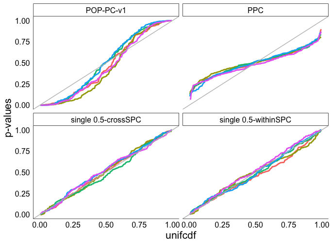
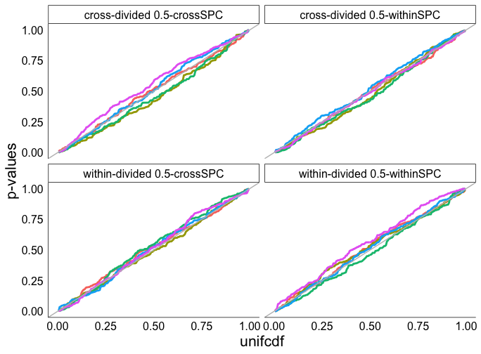
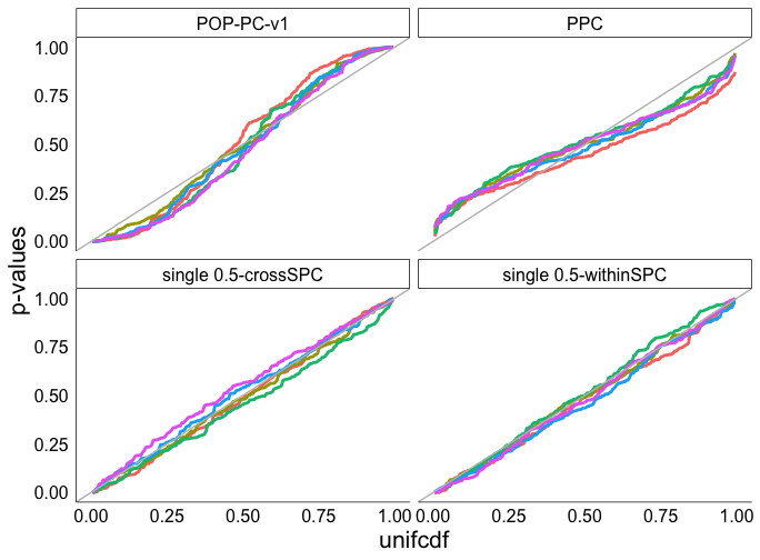
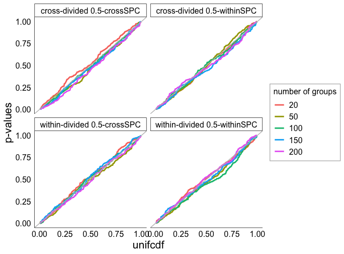
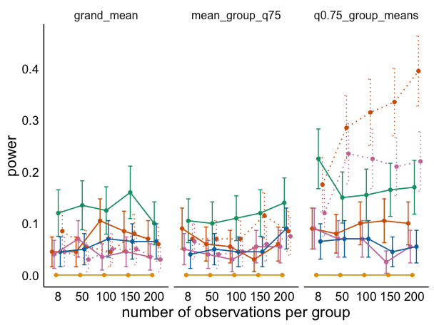
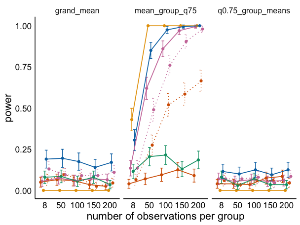
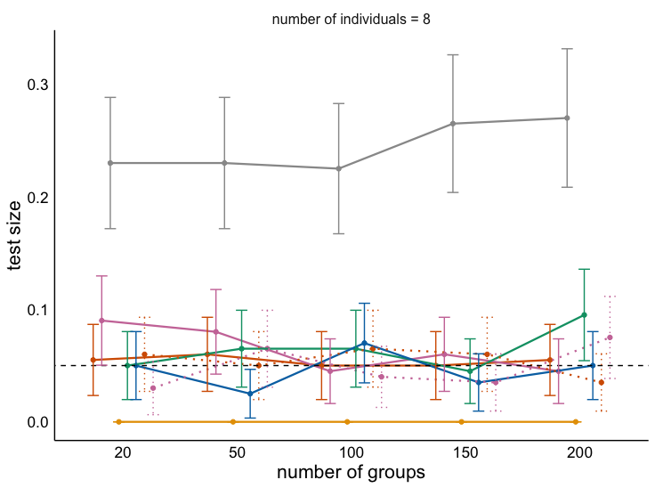
Figures 10a, 10c and 10e show that in the well-specified Scenario 1 for all statistics both single and divided SPCs correctly control test size and produce uniform $p$-values (see also Fig. B.27f). PPCs have the smallest test size but the $p$-values are not uniformly distributed (see also Fig. B.27e) and so are not well-calibrated. For all scenarios POP-PC-v1 fails to control the test size. Hence, we omit POP-PC-v1 in the remainder of the discussion.

(a) grand mean

(b) Scenario 2

(c) mean of 75th quantiles of each group

(d) Scenario 3

(e) 75th quantile of group means

(f) Scenario 4

Figure 10: Test size (a,c,e) and power (b,d,f) plots for different checks and statistics given fixed number of individuals $J=8$ and increasing number of groups $I\in\{20,50,100,150,200\}$ under Gaussian hierarchical model. The test size is estimated by repeatedly generating data from well-specified model for 200 times and run each candidate check in each iteration to get their corresponding $p$-values. Powers are estimated with 200 repeated experiments for each scenario. Vertical bars represnet the $95$th confidence intervals for the estimation. The horizontal dashed line indicates significance level $\alpha=0.05$. Dotted lines are divided SPC using within splitting strategy to get $k$ folds as discussed in Section 4.

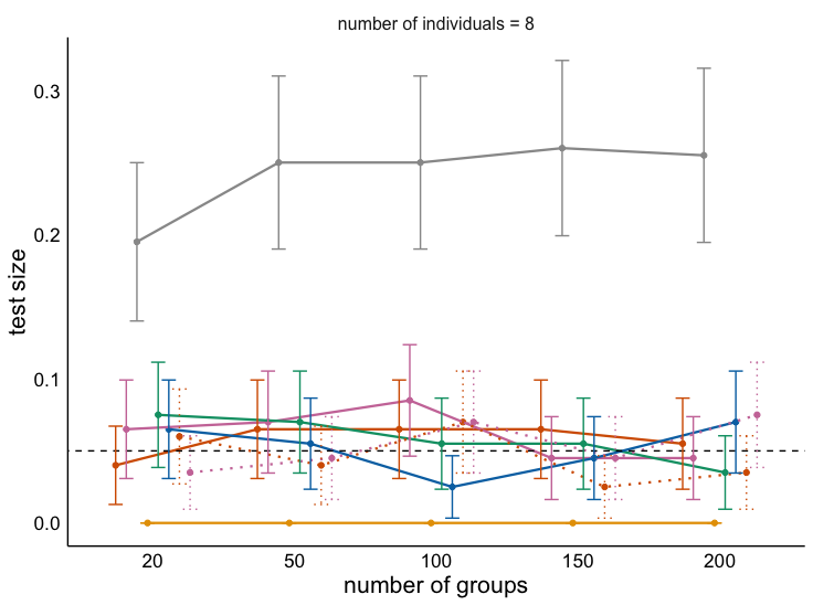
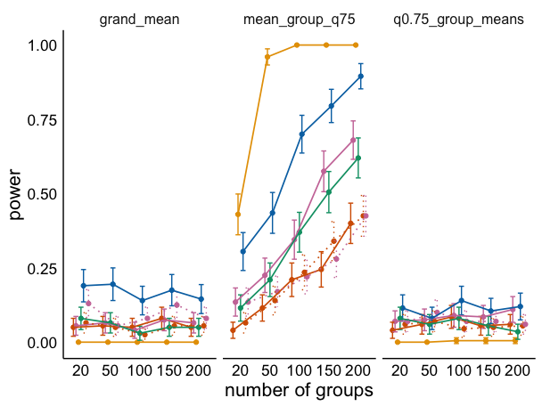
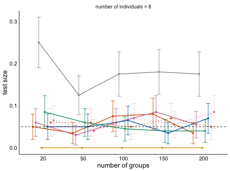
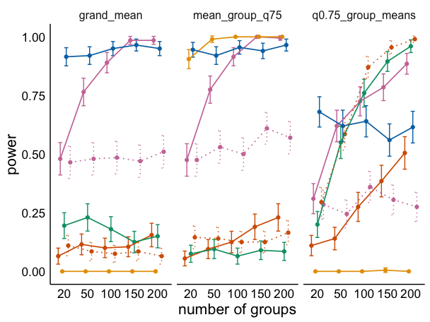
Power

As discussed in Section 4, a hierarchical structure may produce different levels of misspecification for which only certain test statistics and checking methods will be effective.

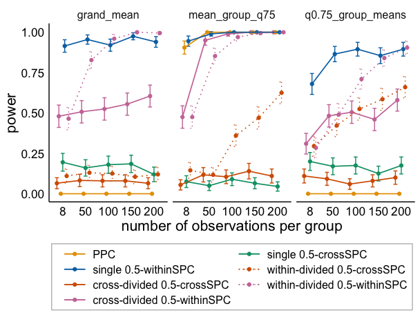
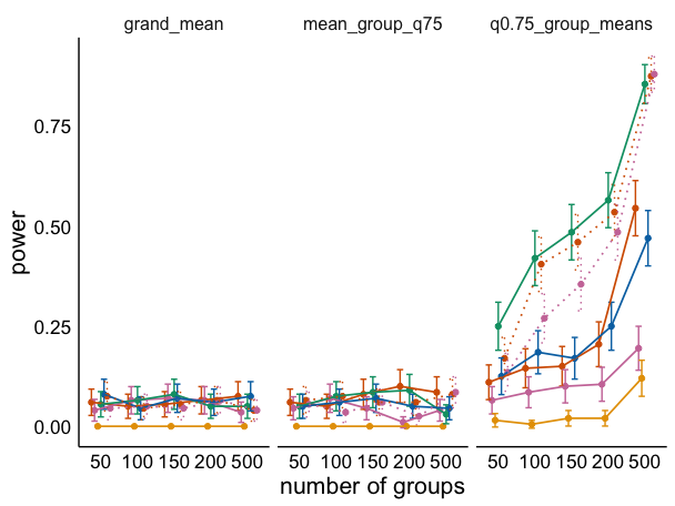
Scenario 2 introduces misspecification between groups, which is most effectively detected by the $75$th quantile of group means statistic. Figure 10b shows that, both single and divided SPCs dramatically outperform PPCs. Also, as suggested in Section 4, cross-SPCs are best for testing for group-level misspecification and cross-divided cross-SPCs have smaller power than within-divided cross-SPCs because doing cross-splits twice in divided SPCs results in poor posterior estimation in a small data regime. single cross-SPCs outperform single within-SPCs.

Scenario 3 introduces observation-level mismatch between the model and data. In this case the mean of group $75$th quantiles statistic is most effective at detecting the misspecification. Figure 10d shows that PPCs outperform the SPCs, although, as suggested in Section 4, the within-SPC methods are also quite effective, with single within-SPC being the best SPC.

Scenario 4 introduces mismatches at both levels and all three statistics are capable of detecting the mismatches. Figure 10f shows that PPCs are only effective when used with the mean of group $75$th quantiles statistic while SPCs are effective for all three statistics. With the mean of group 75th quantiles statistic, which is used to detect the lower-level misspecification, and the grand mean, only the within-SPCs have good power. Further, the cross-divided within-SPC outperforms the within-divided within-SPC due to the small data effects. Similar analysis applies to grand mean statistic. For 75th quantile of group means, which captures the group-level misspecification, cross-SPCs outperform within-SPCs.

6 Experiments

In this section, we compare SPCs to PPCs on four real-data examples. We do not include POP-PC-v1s in our comparison due to their lack of test size control in some of the simulation results.

6.1 Light speed data

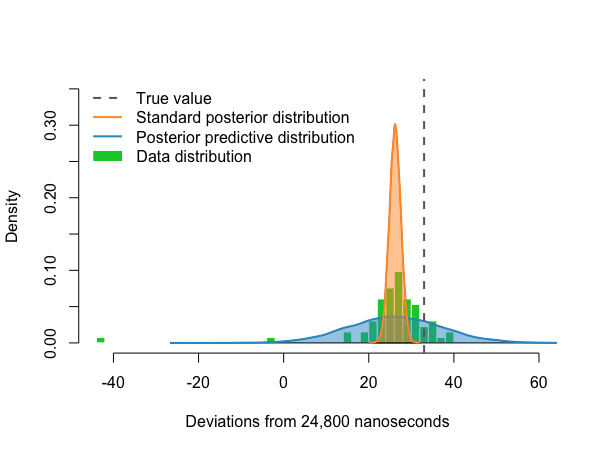
The light speed data is discussed in both Gelman et al. (2013) and Robins, van der Vaart and Ventura (2000). The data were collected by Simon Newcomb (1882), who measured the time that light takes to travel 7442 meters at sea level. The observations are recorded as deviations from 24800 nanoseconds and $N=66$. We consider a normal model $P_{\theta}=\mathcal{N}(\mu,\sigma^{2})$ with an improper prior density $\pi_{0}(\mu,\sigma^{2})=\sigma^{-2}$. A comparison of the data distribution and the posterior predictive distribution is displayed in Fig. 11a, which shows that the model does not capture the heavy left tail of the data and that the 95% posterior credible interval does not contain the true value. We consider five statistics: mean, standard deviation, MSE, $5$th and $95$th quantiles. We use $q=0.5$ to ensure the statistics (particularly the quantiles) can be reasonably estimated. Two-sided $p$-values computed for each method and statistic are given in Table 1. Both the PPC and single SPC yield small $p$-values for the left quantile. The single SPC yields a small $p$-value for the standard deviation and MSE while the PPC results in a small $p$-value for the right quantile. Thus, we find that the single SPC captures complementary (but overlapping) forms of misspecification compared to the PPC. On the other hand, as expected in this small-data regime, the divided SPCs yield $p$-values far from zero.

(a) light speed data

(b) airline delays data

Figure 11: (a) displays the histogram of light data, the standard posterior and posterior prediction density curves. The vertical dashed line is the “true value” based on the currently accepted value of speed of light, $\nu=33.0$. (b) shows the histograms of airline delays data and $N=327,346$ posterior predictive draws under simple geometric model (Geom) and negative binomial generalized linear model (NB/GLM) with counts in $\log$ scale.

Table 1: Two-sided $p$-values for light data.

Methods/ Statistics	5th quantile	Mean	95th quantile	Std Dev	MSE
PPC	0.004	0.996	0.010	0.944	0.894
single 0.5-SPC	0.012	0.608	0.762	0.000	0.000
divided 0.5-SPC, $k=\lfloor N^{0.49}\rfloor$	0.592	0.533	0.259	0.239	0.200

6.2 Airline delays data: geometric model

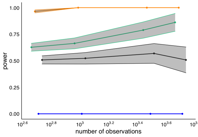
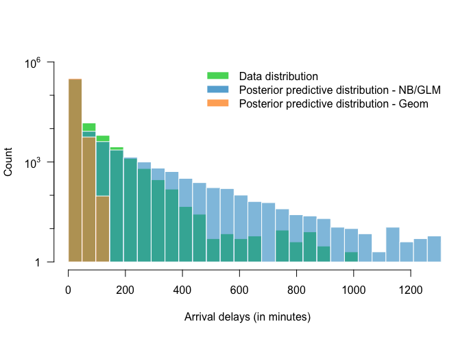
We investigate the power of the single and divided SPCs compared to the PPC using the airline on-time data for all flights departing NYC in 2013. Suppose we want to model $y=\max(\texttt{arr\_delay}-15,0)$, delay duration over 15 minutes for all delayed flights. We assume a geometric model $y\sim{\sf{Geom}}(\theta)$ with conjugate prior $p\sim{\sf{Beta}}(0.1,0.2)$. A comparison of observed data distribution and posterior predictive distribution is shown in Fig. 11b, which shows that model fails to capture the heavy right tail of the data distribution. Thus, we should expect statistics sensitive to right tail behavior to reject the assumed model. In particular, we consider the success rate statistic $T(\mathbf{X}):=N/\sum_{n=1}^{N}X_{n}$ and the MSE statistic. To estimate the power of all checks across different dataset sizes, we permute and segment the full dataset into $I:=\lfloor N/N_{\text{sub}}\rfloor$ disjoint subsets of equal size $N_{\text{sub}}\in\{500,1000,2000,3000,5000\}$. Each subset is regarded as an “original observed data” and all candidate checks are applied to produce one $p$-value for each dataset, from which we can estimate the power at a fixed test size.

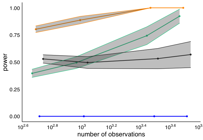
Figure 12 shows that while all checks perform well for the MSE statistic, only the SPCs (with $q=0.5$) have large powers for the success rate statistic. These results also establish the practical value of the divided SPC, which with $k=N_{\text{sub}}^{0.49}$ rapidly reaches power of one while PPC has power 0 and single SPC has approximately constant power of around 0.5 across sample sizes. Notably, divided SPC with a lower rate $k=N_{\text{sub}}^{0.39}$ has increasing power but worse power than with $k=N_{\text{sub}}^{0.49}$. Figure B.28 shows similar results for SPCs with $q=0.9$.

(a) Success rate

(b) MSE

Figure 12: The power estimates for PPC and SPCs with proportion $q=0.5$ of NYC airline data using a geometric model. The power is estimated by segmenting the full dataset into subsets of equal sizes $N_{\text{sub}}\in\{500,1000,2000,3000,5000\}$ and computing $p$-values for each subset. The shaded region represents $95\%$ confidence intervals for the power estimation.

6.3 Airline delays data: negative binomial regression

To illustrate the flexibility of SPCs for structured models compared to PPCs, we next consider a negative binomial regression model for the airline delays data with covariates $\sin(\texttt{Month}/12)$, $\cos(\texttt{Month}/12)$, $\sin(\texttt{DayOfWeek}/7)$, $\cos(\texttt{DayOfWeek}/7)$, and Distance (between airports). As discussed in Section 4, in a time-series model, there are two possible types of splitting, interpolated and extrapolated. Figure 11b shows that the negative binomial generalized linear model explains the data fairly well, although the tail of the predictive distribution is heavier than the data. Hence, it is not immediately clear which predictive checks pass. From Table 2 we see that, in fact, interpolated single SPC and PPC $p$-values are large, while the extrapolated single SPC $p$-value indicates the model does not predict future data well. On the other hand, the more sensitive divided SPC picks up on misspecification not just in the extrapolation setting but for interpolation as well. These results suggest the success rate misspecification is fairly subtle. Depending on the use case, these insights could guide whether further model elaboration is necessary.

Table 2: Two-sided p-values of different split types in SPCs of $q=0.5$ under negative binomial regression model with airline data and success rate statistic.

Methods	P-values
PPC	0.132
Interpolated single 0.5-SPC	0.626
Extrapolated single 0.5-SPC	0.000
Double-interpolated divided 0.5-SPC, $k=N^{0.49}$	0.000
Interpolated divided extrapolated 0.5-SPC, $k=N^{0.49}$	0.001

6.4 Birthday model

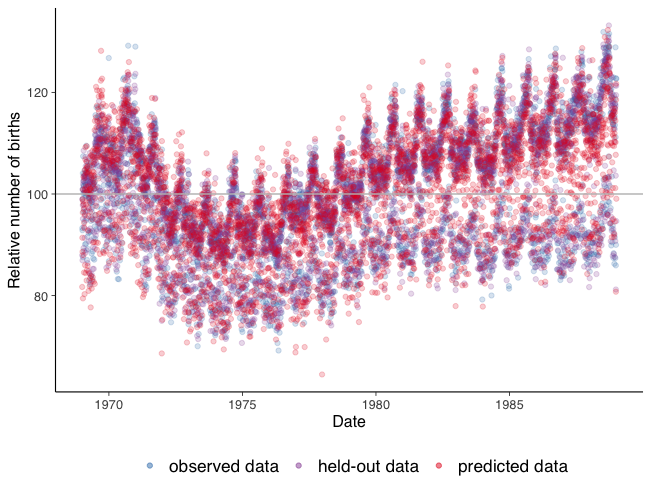
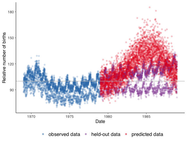
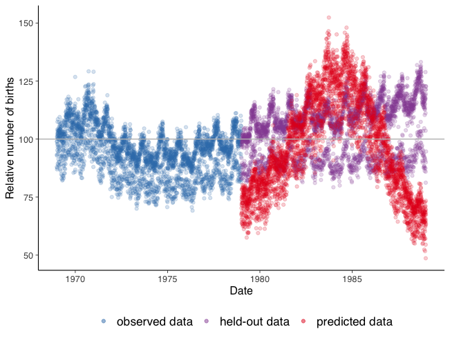
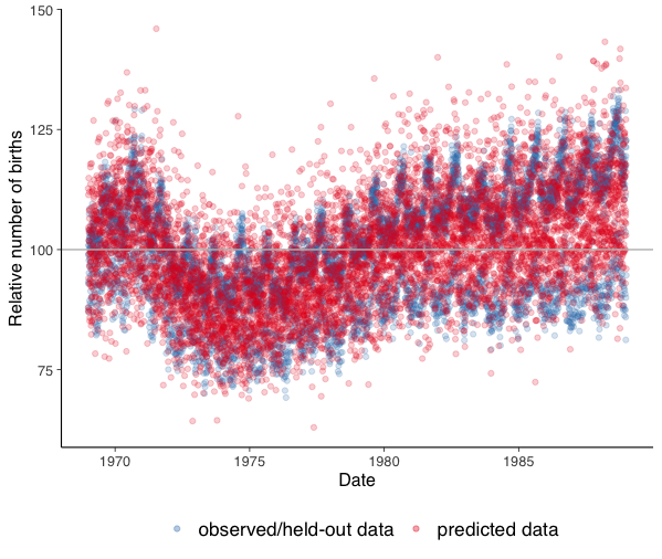
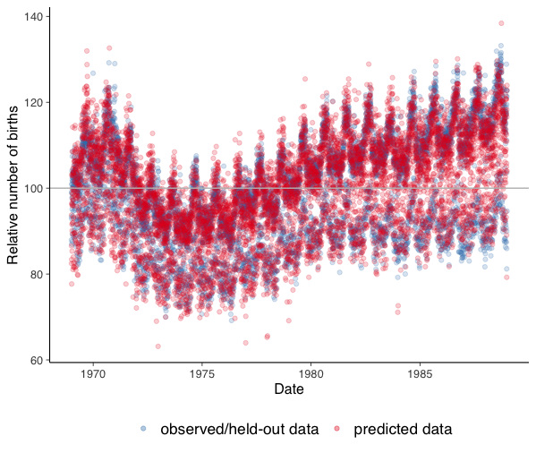
The birthday data consists of the number of births per day in the United Stats for the years 1969–1988. We discuss two Gaussian process models from Gelman et al. (2013, Chap. 21.2, pp. 507): Model 1 fits the long-term trend using an exponentiated quadratic kernel $k(x,x^{\prime})=\sigma^{2}\exp(-\frac{\|x-x^{\prime}\|^{2}}{2c^{2}})$; Model 6 uses a carefully designed kernel which contains seasonal, day-of-week, and day-of-year effects. To assess how well the model captures the correlation structure of the time-series data, we employ graphical checks as well as lag 1 to 30 autocorrelation coefficients as statistics for computing $p$-values.

Model 1

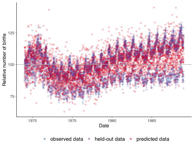
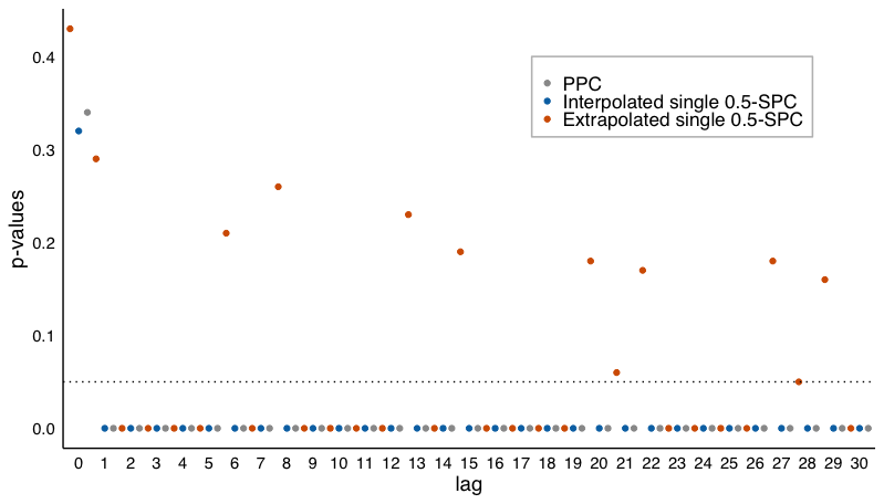
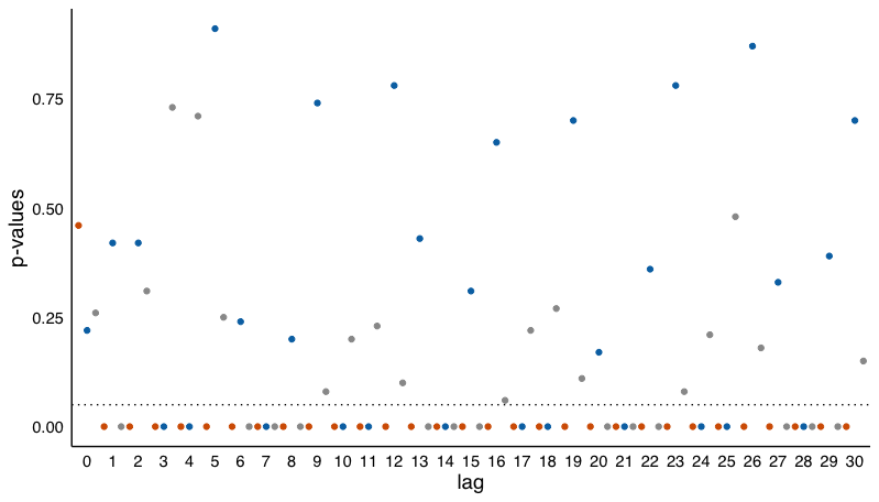
The graphical predictive checks in Fig. 13 indicate that, for Model 1, interpolation (interpolated single SPC, Fig. 13a) and replication (PPC, Fig. 13e) generate some outliers and fail to capture the two “bands” of data, with many predicted observations between the two bands. The accuracy of extrapolation (extrapolated single SPC, Fig. 13c) appears quite poor. The apparent inadequacies of Model 1 are confirmed by the $p$-values for all three predictive checks, as shown in Fig. 14a. Notably, however, the extrapolated single SPC fails to reject for lags equal to $7i\pm 1$ for $i\in\{0,1,2,3,4\}$, which suggests a potential improvement to Model 1 by adding day-of-week effects.

Model 6

The graphical checks for Model 6 indicate that for interpolation (Fig. 13b) and replication (Fig. 13f) the fit is better than for Model 1, with noticeably fewer outliers and predicted observations between the two bands. However, the accuracy of extrapolation (Fig. 13d) remains quite poor. The findings of the graphical checks are generally confirmed by the $p$-values shown in Fig. 14b: for many lags PPC and interpolated single SPC fail to reject while the extrapolated single SPC rejects for all lags greater than zero.

(a) Model 1, interpolated single 0.5-SPC

(b) Model 6, interpolated single 0.5-SPC

(c) Model 1, extrapolated single 0.5-SPC

(d) Model 6, extrapolated single 0.5-SPC

(e) Model 1, PPC

(f) Model 6, PPC

Figure 13: The scatter plot of replicated data vs. held-out and original data under Model 1 and Model 6 with PPC, interpolated and extrapolated single 0.5-SPC.

(a) Model 1

(b) Model 6

Figure 14: Two-sided $p$-values for lag-0 to lag-30 auto-correlation coefficients under Models 1 and 6 for the birthday data. We compare interpolated and extrapolated single 0.5-SPCs to PPCs. The horizontal dotted line is the significance level of 0.05.

7 Conclusion

In this paper, we have proposed split predictive checks (SPCs) as an asymptotically well-calibrated complement to posterior predictive checks (PPCs) that retain computational efficiency and general applicability of PPCs. In addition, we have shown how SPCs provide additional flexibility in the context of structured models such as time-series and hierarchical models, which allows the data analyst to design the check to match how the model will be used. There are several interesting directions for future research. Our simulation study and theory for the normal location model suggest the calibration properties of SPCs extend to the case of realized discrepancies, but it would be worthwhile to develop a more comprehensive theory. Such a theory could also cover discrepancies that have non-normal limiting distributions. Since SPCs can become unreliable when the prior is very influential, it could also be fruitful to develop a non-asymptotic theory of SPCs, which might lead to corrections to the $p$-values in the small-sample setting.

Acknowledgments

Thanks to Aki Vehtari and Jeffrey Miller for helpful discussions, and to Jeffrey Negrea for help with conditions for uniform Donsker classes and sharing his preprocessed airline flight delay data. J. Li and J. H. Huggins were supported by the National Institute of General Medical Sciences of the National Institutes of Health under grant number R01GM144963 as part of the Joint NSF/NIGMS Mathematical Biology Program. The content is solely the responsibility of the authors and does not necessarily represent the official views of the National Institutes of Health.

Appendix A Proofs

A.1 Technical lemmas

We state some preliminary definitions and lemmas needed for the proofs of the single SPC-related results Theorems 3.4 and 3.1.

To quantify the distance between probability measures, we rely on a number of different probability metrics: Kolmogorov distance, Wasserstein distance, total variation (TV) distance, and the bounded Lipschitz distance. It follows from the definitions $d_{TV,S}\leq d_{TV}$ and $d_{K}\leq d_{TV}$. The $s$-Wasserstein distance between distributions $\mu$ and $\nu$ defined on $\Omega\subseteq\mathbb{R}^{d}$ is given by $W_{s}(\mu,\nu):=\inf_{\xi}\{\int|u-v|^{s}\xi(\mathrm{d}u,\mathrm{d}v)\}^{1/s}$, where the infimum is over all distributions on $\Omega\times\Omega$ with marginals $\mu$ and $\nu$; that is, with $\xi(\cdot,\mathbb{R})=\mu$ and $\xi(\mathbb{R},\cdot)=\omega$ (Villani, 2009). By Gibbs and Su (2002, Theorem 4.1), we have

$$W_{s}(\mu,\nu)\leq\operatorname{diam}(\Omega)\,d_{TV}(\mu,\nu).$$ (15)

If $d=1$, by Bouchitte, Jimenez and Mahadevan (2007, Theorem 1.2), we have

$$d_{K}(\mu,\nu)\leq C_{s}W^{\frac{s}{1+s}}_{s}(\mu,\nu),$$ (16)

where $\operatorname{diam}(\Omega):=\sup\{|x-y|:x,y\in\Omega\}$ and $C_{s}$ is a constant depending on $s\geq 1$.

For a function $f:\mathbb{R}^{d}\to\mathbb{R}$, let $\left\|{f}\right\|_{L}=\sup_{a\neq b}\frac{|f(a)-f(b)|}{\left\|{a-b}\right\|_{2}}$ denote the Lipschitz constant of $f$ and let $\left\|{f}\right\|_{\infty}=\sup_{a}|f(a)|$. Define norm $\|\cdot\|_{BL}$ for all bounded and Lipschitz continuous functions $f$ as $\|f\|_{BL}:=\|f\|_{\infty}+\|f\|_{L}$. The bounded Lipschitz distance is given by

$$d_{BL}(X,Y):=\sup_{h:\|h\|_{BL}\leq 1}\left|\mathbb{E}\{h(X)\}-\mathbb{E}\{h(Y)\}\right|.$$ (17)

Further, we can show that the Kolmogorov distance between two pairs of convolutions can be upper bounded by a combination of a bounded Lipschitz metric and Kolmogorov distance between single random variables. We present it as a lemma below.

Lemma A.1.

Suppose $X$, $Y$, $\tilde{X}$ and $\tilde{Y}$ are independent random variables. Assume that $F_{\tilde{Y}}$, the CDF of $\tilde{Y}$, satisfies $\|F_{\tilde{Y}}\|_{BL}<\infty$. Then

$$d_{K}(\tilde{X}+\tilde{Y},X+Y)\leq\|F_{\tilde{Y}}\|_{BL}d_{BL}(\tilde{Y},Y)+d_{K}(\tilde{X},X).$$ (18)

Proof.

Let $F_{\tilde{X}}$, $F_{X}$, $F_{Y}$ denotes the CDFs of, respectively, $\tilde{X}$, $X$ and $Y$. By definition of convolutions and Kolmogorov distance,

$$d_{K}\left(\tilde{X}+\tilde{Y},X+Y\right)$$ (19)

$$=\sup_{t\in\mathbb{R}}\left|\int_{\mathbb{R}}F_{\tilde{X}}(t-y)\mathrm{d}F_{\tilde{Y}}(y)-\int_{\mathbb{R}}F_{X}(t-y)\mathrm{d}F_{Y}(y)\right|$$ (20)

$$\leq\sup_{t\in\mathbb{R}}\left|\int_{\mathbb{R}}F_{\tilde{X}}(t-y)\mathrm{d}F_{\tilde{Y}}(y)-\int_{\mathbb{R}}F_{\tilde{X}}(t-y)\mathrm{d}F_{Y}(y)\right|+\sup_{t\in\mathbb{R}}\left|\int_{\mathbb{R}}F_{X}(t-y)-F_{\tilde{X}}(t-y)\mathrm{d}F_{Y}(y)\right|$$ (21)

$$\leq\sup_{t\in\mathbb{R}}\left|\mathbb{E}\left[F_{\tilde{X}}(t-\tilde{Y})-F_{\tilde{X}}(t-Y)\right]\right|+\sup_{t,y\in\mathbb{R}}\left|F_{X}(t-y)-F_{\tilde{X}}(t-y)\right|\int_{\mathbb{R}}\mathrm{d}F_{Y}(y)$$ (22)

$$=\sup_{t\in\mathbb{R}}\left|\mathbb{E}\left[F_{\tilde{X}}(t-\tilde{Y})-F_{\tilde{X}}(t-Y)\right]\right|+d_{K}(\tilde{X},X)$$ (23)

$$\leq\|F_{\tilde{Y}}\|_{BL}\sup_{f:\|f\|_{BL}<\infty}\left|\mathbb{E}\left[f(\tilde{Y})-f(Y)\right]\right|+d_{K}(\tilde{X},X)$$ (24)

$$=\|F_{\tilde{Y}}\|_{BL}d_{BL}(\tilde{Y},Y)+d_{K}(\tilde{X},X).$$ (25)

∎

Lemma A.2.

Let $\tilde{\theta}_{N}\in\Theta_{N}:=\{\theta:\|\theta-\theta_{\star}\|\leq CR_{N}\}$ for some constant $C>0$ and a sequence $R_{N}>0$ depending on sample size $N$. If Assumption (A1-b) holds, then there exists an absolute constant $c_{2}>0$ such that

$$\left|\frac{N^{1/2}\{\nu(\tilde{\theta}_{N})-\nu(\theta_{\star})\}}{\sigma(\theta_{\star})}-\dot{\nu}(\theta_{\star})^{\top}\frac{N^{1/2}\{\tilde{\theta}_{N}-\theta_{\star}\}}{\sigma(\theta_{\star})}\right|<\frac{c_{2}N^{1/2}R_{N}^{2}}{\sigma(\theta_{\star})}.$$ (26)

Proof.

By Assumption (A1-b), we have $\|\ddot{\nu}(\theta_{\star})\|_{2}=\lambda_{\max}(\ddot{\nu}(\theta_{\star}))<\infty$. Consider the first-order Taylor expansion of $\nu(\tilde{\theta}_{N})$ around $\theta_{\star}$, for some constant $c_{2}>C\lambda_{\max}(\ddot{\nu}(\theta_{\star}))$ and $\theta^{\prime}\in\mathcal{U}(\theta_{\star},\tilde{\theta}_{N}):=\{\theta:\|\theta-\theta_{\star}\|\leq\|\tilde{\theta}_{N}-\theta_{\star}\|\}$,

$$\left|\nu(\tilde{\theta}_{N})-\nu(\theta_{\star})+\dot{\nu}(\theta_{\star})(\tilde{\theta}_{N}-\theta_{\star})\right| =\left|\frac{(\theta^{\prime}-\theta_{\star})^{\top}\ddot{\nu}(\theta_{\star})(\theta^{\prime}-\theta_{\star})}{2}\right|$$ (27)

$$\leq\frac{1}{2}\lambda_{\max}(\ddot{\nu}(\theta_{\star}))\|\theta^{\prime}-\theta_{\star}\|^{2}$$ (28)

$$\leq C\lambda_{\max}(\ddot{\nu}(\theta_{\star}))R_{N}^{2}$$ (29)

$$\leq c_{2}R_{N}^{2},$$ (30)

where the first inequality holds since $\ddot{\nu}(\theta_{\star})$ is symmetric. The proof is complete after multiplying both sides by $N^{1/2}/\sigma(\theta_{\star})$. ∎

Lemma A.3.

(Gaussian Concentration, (Vershynin, 2018, Chap 2.5)) Let $X\sim\mathcal{N}(0,v)$. Then, for all $t\geq 0$,

$$\mathbb{P}\left[|X|\geq t\right]\leq 2e^{-\frac{t^{2}}{2v}}.$$ (31)

Lemma A.4.

Let $\Theta_{N}:=\{\theta:\|\theta-\theta_{\star}\|<C\log^{1/2}N/N^{1/2}\}$. If Assumption A4 holds, then $\mathbb{P}_{\theta_{\star}}\left[\left|\Pi(\Theta_{N}\,|\,\mathbf{X}_{N})-1\right|>cN^{-1/2}\right]=O(N^{-s/2})$.

Proof.

It follows from Lemma A.3 and Assumption (A4-a) that $\mathbb{P}_{\theta_{\star}}[|\widehat{\Pi}(\Theta_{N}\,|\,\mathbf{X}_{N})-1|>CN^{-1}]=O(N^{-s/2})$. Combining this inequality with Assumption (A4-b) yields

$$\mathbb{P}_{\theta_{\star}}\left[\left|\Pi(\Theta_{N}\,|\,\mathbf{X}_{N})-1\right|>cN^{-1/2}\right]$$ (32)

$$\leq\mathbb{P}_{\theta_{\star}}\left[\big{|}\Pi(\Theta_{N}\,|\,\mathbf{X}_{N})-\widehat{\Pi}(\Theta_{N}\,|\,\mathbf{X}_{N})\big{|}+\big{|}\widehat{\Pi}(\Theta_{N}\,|\,\mathbf{X}_{N})-1\big{|}>cN^{-1/2}\right]$$ (33)

$$\leq\mathbb{P}_{\theta_{\star}}\left[d_{TV,\Theta_{N}}\left(\Pi(\cdot\,|\,\mathbf{X}_{N}),\widehat{\Pi}(\cdot\,|\,\mathbf{X}_{N})\right)>cN^{-1/2}-CN^{-1}\right]+O(N^{-s/2})$$ (34)

$$\leq\mathbb{P}_{\theta_{\star}}\left[d_{TV,\Theta_{N}}\left(\Pi(\cdot\,|\,\mathbf{X}_{N}),\widehat{\Pi}(\cdot\,|\,\mathbf{X}_{N})\right)>c_{\mathcal{K}}N^{-1/2}\right]+O(N^{-s/2})$$ (35)

$$\leq\mathbb{P}_{\theta_{\star}}\left[d_{TV,\mathcal{K}}\left(\Pi(\cdot\,|\,\mathbf{X}_{N}),\widehat{\Pi}(\cdot\,|\,\mathbf{X}_{N})\right)>c_{\mathcal{K}}N^{-1/2}\right]+O(N^{-s/2})$$ (36)

$$=O(N^{-s/2}),$$ (37)

where the penultimate inequality follows by $d_{\text{TV},\Theta_{N}}\leq d_{\text{TV},\mathcal{K}}$ since $\Theta_{N}\subset\mathcal{K}$. ∎

Lemma A.5.

If Assumption (A1-c) holds, then for any $\theta\in\Theta_{N}$ defined in Lemma A.2,

$$\left|\frac{\sigma(\theta)}{\sigma(\theta_{\star})}-1\right|\leq\frac{CMR_{N}}{\sigma(\theta_{\star})}.$$ (38)

Proof.

By Taylor’s theorem, for any $\theta\in\Theta_{N}$, there exists a $\theta^{\prime}\in\mathcal{U}(\theta_{\star},\theta):=\{\theta^{\prime}:\|\theta^{\prime}-\theta_{\star}\|\leq\|\theta-\theta_{\star}\|\}$ such that

$$\sigma(\theta)=\sigma(\theta_{\star})+(\theta-\theta_{\star})^{\top}\dot{\sigma}(\theta^{\prime}).$$ (39)

Since $\Theta_{N}\subseteq U_{\theta_{\star}}$, it follows from Assumption (A1-c) together with Eq. 39 that

$$\left|\frac{\sigma(\theta)}{\sigma(\theta_{\star})}-1\right| =|(\theta-\theta_{\star})^{\top}\dot{\sigma}(\theta^{\prime})|/\sigma(\theta_{\star})$$ (40)

$$\leq\left\|{\theta-\theta_{\star}}\right\|_{2}\left\|{\dot{\sigma}(\theta^{\prime})}\right\|/\sigma(\theta_{\star})$$ (41)

$$\leq\frac{CMR_{N}}{\sigma(\theta_{\star})}.$$ (42)

∎

A.2 Proof of Theorem 3.1

Consider the single SPC $p$-value as a random variable

$$p_{\text{SPC}}(\mathbf{X})=\int_{\Theta}\mathbb{P}\left[T_{N_{\text{ho}}}(\mathbf{X}_{\text{pred}})<T_{N_{\text{ho}}}(\mathbf{X}_{\text{ho}})\,|\,\theta\right]\Pi(\mathrm{d}\theta\,|\,\mathbf{X}_{\text{obs}}).$$ (43)

Let $Z$ denote a standard normal random variable and $\phi(\cdot;\mu,\sigma^{2})$ denote the PDF of normal random variables with mean $\mu$ and variance $\sigma^{2}$. Let $\widehat{\pi}(\cdot\,|\,\mathbf{X}_{\text{obs}}):=\phi(\cdot;\hat{\theta}(\mathbf{X}_{\text{obs}}),J_{\star}^{-1}/N_{\text{obs}})$ and $\widehat{\Pi}(\cdot\,|\,\mathbf{X}_{\text{obs}})$ be the corresponding distribution. Denote shrinking parameter space as $\Theta_{N_{\text{obs}}}:=\{\theta:\|\theta-\theta_{\star}\|\leq c{N_{\text{obs}}}^{-1/2}\}$. We emphasize on the difference between asymptotic means and standard deviations of $T_{N}$ by defining $\nu(\theta)$ and $\sigma(\theta)$ as under $P_{\theta}$ and $\nu_{\circ}$ and $\sigma_{\circ}$ as under $P_{\circ}$ respectively. We denote the ratio between asymptotic standard deviations under $P_{\circ}$ and $P_{\theta_{\star}}$ as $\kappa:=\sigma_{\circ}/\sigma(\theta_{\star})$. For simplicity, we introduce some shorthand notation:

$$p^{\prime}_{\text{SPC}}(\mathbf{X}):=\int_{\Theta}\mathbb{P}\left[T_{N_{\text{ho}}}(\mathbf{X}_{\text{pred}})<T_{N_{\text{ho}}}(\mathbf{X}_{\text{ho}})\,|\,\theta\right]\widehat{\Pi}(\mathrm{d}\theta\,|\,\mathbf{X}_{\text{obs}})$$ (44)

$$p^{\prime\prime}_{\text{SPC}}(\mathbf{X}):=\int_{\Theta_{N_{\text{obs}}}}\mathbb{P}\left[T_{N_{\text{ho}}}(\mathbf{X}_{\text{pred}})<T_{N_{\text{ho}}}(\mathbf{X}_{\text{ho}})\,|\,\theta\right]\widehat{\Pi}(\mathrm{d}\theta\,|\,\mathbf{X}_{\text{obs}})$$ (45)

$$s_{T\nu}(\mathbf{X};\theta,N):=N^{1/2}\{T_{N}(\mathbf{X})-\nu(\theta)\}$$ (46)

$$s_{T\nu_{\circ}}(\mathbf{X};N):=N^{1/2}\{T_{N}(\mathbf{X})-\nu_{\circ}\}$$ (47)

$$\xi(\theta):=\mathbb{P}\big{[}s_{T\nu}(\mathbf{X}_{\text{pred}};\theta,N_{\text{ho}})+N_{\text{ho}}^{1/2}\{\nu(\theta)-\nu(\theta_{\star})\}>s_{T\nu_{\circ}}(\mathbf{X}_{\text{pred}};N_{\text{ho}})+N_{\text{ho}}^{1/2}\{\nu_{\circ}-\nu(\theta_{\star})\}\,|\,\theta\big{]}$$ (48)

$$t(\theta):=\frac{s_{T\nu_{\circ}}(\mathbf{X}_{\text{ho}};N_{\text{ho}})}{\sigma_{\circ}}\kappa-\frac{N_{\text{ho}}^{1/2}\dot{\nu}(\theta_{\star})\{\theta-\theta_{\star}\}}{\sigma(\theta_{\star})}+\frac{N_{\text{ho}}^{1/2}\{\nu_{\circ}-\nu(\theta_{\star})\}}{\sigma(\theta_{\star})}$$ (49)

$$Q(\mathbf{X}_{\text{ho}},\mathbf{X}_{\text{obs}}):=\frac{1}{\tilde{\sigma}}\left(\frac{s_{T\nu_{\circ}}(\mathbf{X}_{\text{ho}};N_{\text{ho}})}{\sigma_{\circ}}\kappa-\frac{N_{\text{ho}}^{1/2}}{N_{\text{obs}}^{1/2}}\frac{N_{\text{obs}}^{1/2}\dot{\nu}(\theta_{\star})\{\hat{\theta}(\mathbf{X}_{\text{obs}})-\theta_{\star}\}}{\sigma(\theta_{\star})}+\frac{N_{\text{ho}}^{1/2}\{\nu_{\circ}-\nu(\theta_{\star})\}}{\sigma(\theta_{\star})}\right).$$ (50)

Assume that $N_{\text{obs}}$ is sufficiently large such that $\Theta_{N_{\text{obs}}}\subseteq\mathcal{U}_{\star,1}\cap\mathcal{U}_{\star,2}$. Letting $t=\Omega(N_{\text{obs}}^{-1/2})$ and $v=O(N_{\text{obs}}^{-1})$ for Lemma A.3 gives that $\widehat{\Pi}(\Theta_{N_{\text{obs}}}\,|\,\mathbf{X}_{\text{obs}})\overset{P}{\to}1$. By Assumption (A3-b), Lemma A.3 and the fact that $d_{TV}(\mu,\omega):=2\sup_{f\in[0,1]}|\int f\mathrm{d}\mu-\int f\mathrm{d}\omega|$, we have

$$\left|p_{\text{SPC}}(\mathbf{X})-p^{\prime\prime}_{\text{SPC}}(\mathbf{X})\right| \leq\left|p_{\text{SPC}}(\mathbf{X})-p^{\prime}_{\text{SPC}}(\mathbf{X})\right|+\left|p^{\prime}_{\text{SPC}}(\mathbf{X})-p^{\prime\prime}_{\text{SPC}}(\mathbf{X})\right|$$ (51)

$$\leq d_{TV}\left(\Pi(\cdot\mid\mathbf{X}_{\text{obs}}),\widehat{\Pi}(\cdot\,|\,\mathbf{X}_{\text{obs}})\right)+\widehat{\Pi}(\Theta^{c}_{N_{\text{obs}}}\,|\,\mathbf{X}_{\text{obs}})$$ (52)

$$\overset{P}{\to}0.$$ (53)

By centering both $T_{N_{\text{ho}}}(\mathbf{X}_{\text{pred}})$ and $T_{N_{\text{ho}}}(\mathbf{X}_{\text{ho}})$, the integrand of $p^{\prime\prime}_{\text{SPC}}(\mathbf{X})$ becomes

$$\mathbb{P}\left[T_{N_{\text{ho}}}(\mathbf{X}_{\text{pred}})>T_{N_{\text{ho}}}(\mathbf{X}_{\text{ho}})\,|\,\theta\right]$$ (54)

$$=\mathbb{P}\big{[}N_{\text{ho}}^{1/2}\{T_{N_{\text{ho}}}(\mathbf{X}_{\text{pred}})-\nu(\theta)\}+N_{\text{ho}}^{1/2}\{\nu(\theta)-\nu(\theta_{\star})\}$$ (55)

$$\hskip 42.67912pt>N_{\text{ho}}^{1/2}\left\{T_{N_{\text{ho}}}(\mathbf{X}_{\text{ho}})-\nu_{\circ}\right\}+N_{\text{ho}}^{1/2}\{\nu_{\circ}-\nu(\theta_{\star})\}\,|\,\theta\big{]}$$ (56)

$$=\mathbb{P}\big{[}s_{T\nu}(\mathbf{X}_{\text{pred}};\theta,N_{\text{ho}})+N_{\text{ho}}^{1/2}\{\nu(\theta)-\nu(\theta_{\star})\}$$ (57)

$$\hskip 42.67912pt>s_{T\nu_{\circ}}(\mathbf{X}_{\text{pred}};N_{\text{ho}})+N_{\text{ho}}^{1/2}\{\nu_{\circ}-\nu(\theta_{\star})\}\,|\,\theta\big{]}$$ (58)

$$=:\xi(\theta).$$ (59)

Dividing by $1/\sigma(\theta_{\star})$ on both sides within the probability and applying Lemmas A.5 and A.2 with $R_{N}=CN_{\text{obs}}^{-1/2}$ yields

$$\xi(\theta) \leq\mathbb{P}\big{[}s_{T\nu}(\mathbf{X}_{\text{pred}};\theta,N_{\text{ho}})+\frac{N_{\text{ho}}^{1/2}}{N_{\text{obs}}^{1/2}}\left(N_{\text{obs}}^{1/2}\dot{\nu}(\theta_{\star})\{\theta-\theta_{\star}\}+C/N_{\text{obs}}^{1/2}\right)$$ (60)

$$\hskip 42.67912pt>s_{T\nu_{\circ}}(\mathbf{X}_{\text{ho}};N_{\text{ho}})+N_{\text{ho}}^{1/2}\{\nu_{\circ}-\nu(\theta_{\star})\}\,|\,\theta\big{]}$$ (61)

$$=\mathbb{P}\big{[}s_{T\nu}(\mathbf{X}_{\text{pred}};\theta,N_{\text{ho}})+N_{\text{ho}}^{1/2}\dot{\nu}(\theta_{\star})\{\theta-\theta_{\star}\}+CN_{\text{ho}}^{1/2}/N_{\text{obs}}$$ (62)

$$\hskip 42.67912pt>s_{T\nu_{\circ}}(\mathbf{X}_{\text{ho}};N_{\text{ho}})+N_{\text{ho}}^{1/2}\{\nu_{\circ}-\nu(\theta_{\star})\}\,|\,\theta\big{]}$$ (63)

$$=\mathbb{P}\bigg{[}\frac{s_{T\nu}(\mathbf{X}_{\text{pred}};\theta,N_{\text{ho}})}{\sigma(\theta)}\frac{\sigma(\theta)}{\sigma(\theta_{\star})}+\frac{N_{\text{ho}}^{1/2}\dot{\nu}(\theta_{\star})\{\theta-\theta_{\star}\}}{\sigma(\theta_{\star})}+\frac{CN_{\text{ho}}^{1/2}/N_{\text{obs}}}{\sigma(\theta_{\star})}$$ (64)

$$\hskip 42.67912pt>\frac{s_{T\nu_{\circ}}(\mathbf{X}_{\text{ho}};N_{\text{ho}})}{\sigma_{\circ}}\frac{\sigma_{\circ}}{\sigma(\theta_{\star})}+\frac{N_{\text{ho}}^{1/2}\{\nu_{\circ}-\nu(\theta_{\star})\}}{\sigma(\theta_{\star})}\,|\,\theta\bigg{]}$$ (65)

$$\leq\mathbb{P}\bigg{[}\frac{s_{T\nu}(\mathbf{X}_{\text{pred}};\theta,N_{\text{ho}})}{\sigma(\theta)}\left(1+\frac{CM}{\sigma(\theta_{\star})N_{\text{obs}}^{1/2}}\right)+\frac{N_{\text{ho}}^{1/2}\dot{\nu}(\theta_{\star})\{\theta-\theta_{\star}\}}{\sigma(\theta_{\star})}+\frac{CN_{\text{ho}}^{1/2}/N_{\text{obs}}}{\sigma(\theta_{\star})}$$ (66)

$$\hskip 42.67912pt>\frac{s_{T\nu_{\circ}}(\mathbf{X}_{\text{ho}};N_{\text{ho}})}{\sigma_{\circ}}\kappa+\frac{N_{\text{ho}}^{1/2}\{\nu_{\circ}-\nu(\theta_{\star})\}}{\sigma(\theta_{\star})}\,|\,\theta\bigg{]}$$ (67)

$$=1-\mathbb{P}\bigg{[}\frac{s_{T\nu}(\mathbf{X}_{\text{pred}};\theta,N_{\text{ho}})}{\sigma(\theta)}<\frac{s_{T\nu_{\circ}}(\mathbf{X}_{\text{ho}};N_{\text{ho}})}{\sigma_{\circ}}\kappa$$ (68)

$$\hskip 56.9055pt-\frac{N_{\text{ho}}^{1/2}\dot{\nu}(\theta_{\star})\{\theta-\theta_{\star}\}}{\sigma(\theta_{\star})}+\frac{N_{\text{ho}}^{1/2}\{\nu_{\circ}-\nu(\theta_{\star})\}}{\sigma(\theta_{\star})}\,|\,\theta\bigg{]}+o_{P}(N_{\text{obs}}^{-1/2})$$ (69)

$$=1-\mathbb{P}\bigg{[}\frac{s_{T\nu}(\mathbf{X}_{\text{pred}};\theta,N_{\text{ho}})}{\sigma(\theta)}<t(\theta)\,|\,\theta\bigg{]}+o_{P}(N_{\text{obs}}^{-1/2}).$$ (70)

By Assumption A2, $\frac{s_{T\nu}(\mathbf{X}_{\text{pred}};\theta,N_{\text{ho}})}{\sigma(\theta)}$, we have

$$\left|\mathbb{P}\bigg{[}\frac{s_{T\nu}(\mathbf{X}_{\text{pred}};\theta,N_{\text{ho}})}{\sigma(\theta)}<t(\theta)\,|\,\theta\bigg{]}-\Phi\left(t(\theta);\theta\right)\right|\overset{P}{\to}0.$$ (71)

Combining Eqs. 71, 70 and 59 yields

$$\left|\mathbb{P}\left[T_{N_{\text{ho}}}(\mathbf{X}_{\text{pred}})>T_{N_{\text{ho}}}(\mathbf{X}_{\text{ho}})\,|\,\theta\right]-(1-\Phi\left(t(\theta);\theta\right))\right|\overset{P}{\to}0,$$ (72)

and thus

$$\left|1-p^{\prime\prime}_{\text{SPC}}(\mathbf{X})-\int_{\Theta_{N_{\text{obs}}}}\Phi\left(t(\theta);\theta\right)\widehat{\Pi}(\mathrm{d}\theta\,|\,\mathbf{X}_{\text{obs}})\right|\overset{P}{\to}0,$$ (73)

Let $\mathbb{E}_{\theta}[\cdot]$ denote the expectation with respect to $\phi(\hat{\theta}(\mathbf{X}_{\text{obs}}),J_{\star}^{-1}\Sigma_{\star}J_{\star}^{-1}/N_{\text{obs}})$. Let $Z$ be an independent standard normal random variable and define

$$\tilde{Z} :=Z+\frac{N_{\text{ho}}^{1/2}}{N_{\text{obs}}^{1/2}}\frac{N_{\text{obs}}^{1/2}\dot{\nu}(\theta_{\star})\{\theta-\hat{\theta}(\mathbf{X}_{\text{obs}})\}}{\sigma(\theta_{\star})}\sim\mathcal{N}(0,\tilde{\sigma}^{2}), \quad\text{where }\tilde{\sigma}^{2} :=1+\frac{\frac{N_{\text{ho}}}{N_{\text{obs}}}\dot{\nu}(\theta_{\star})^{2}J_{\star}^{-1}}{\sigma(\theta_{\star})^{2}}.$$ (74)

Consider

$$\int_{\Theta_{N_{\text{obs}}}}\Phi\left(t(\theta);\theta\right)\widehat{\Pi}(\mathrm{d}\theta\,|\,\mathbf{X}_{\text{obs}})$$ (75)

$$=\mathbb{E}_{\theta}\left[\mathbb{P}_{Z}\bigg{[}Z\leq\frac{s_{T\nu_{\circ}}(\mathbf{X}_{\text{ho}};N_{\text{ho}})}{\sigma_{\circ}}\kappa-\frac{N_{\text{ho}}^{1/2}\dot{\nu}(\theta_{\star})\{\theta-\theta_{\star}\}}{\sigma(\theta_{\star})}+\frac{N_{\text{ho}}^{1/2}\{\nu_{\circ}-\nu(\theta_{\star})\}}{\sigma(\theta_{\star})}\bigg{]}\right]$$ (76)

$$=\mathbb{P}_{Z,\theta}\left[Z\leq\frac{s_{T\nu_{\circ}}(\mathbf{X}_{\text{ho}};N_{\text{ho}})}{\sigma_{\circ}}\kappa-\frac{N_{\text{ho}}^{1/2}\dot{\nu}(\theta_{\star})\{\theta-\theta_{\star}\}}{\sigma(\theta_{\star})}+\frac{N_{\text{ho}}^{1/2}\{\nu_{\circ}-\nu(\theta_{\star})\}}{\sigma(\theta_{\star})}\right]$$ (77)

$$=\mathbb{P}_{Z,\theta}\bigg{[}Z+\frac{N_{\text{ho}}^{1/2}}{N_{\text{obs}}^{1/2}}\frac{N_{\text{obs}}^{1/2}\dot{\nu}(\theta_{\star})\{\theta-\hat{\theta}(\mathbf{X}_{\text{obs}})\}}{\sigma(\theta_{\star})}$$ (78)

$$\hskip 42.67912pt\leq\frac{s_{T\nu_{\circ}}(\mathbf{X}_{\text{ho}};N_{\text{ho}})}{\sigma_{\circ}}\kappa-\frac{N_{\text{ho}}^{1/2}}{N_{\text{obs}}^{1/2}}\frac{N_{\text{obs}}^{1/2}\dot{\nu}(\theta_{\star})\{\hat{\theta}(\mathbf{X}_{\text{obs}})-\theta_{\star}\}}{\sigma(\theta_{\star})}+\frac{N_{\text{ho}}^{1/2}\{\nu_{\circ}-\nu(\theta_{\star})\}}{\sigma(\theta_{\star})}\bigg{]}$$ (79)

$$=\mathbb{P}_{\tilde{Z}}\bigg{[}\frac{\tilde{Z}}{\tilde{\sigma}}\leq Q(\mathbf{X}_{\text{ho}},\mathbf{X}_{\text{obs}})\bigg{]}$$ (80)

$$=\Phi\left(Q(\mathbf{X}_{\text{ho}},\mathbf{X}_{\text{obs}})\right).$$ (81)

Combining Eqs. 53, 81 and 73 yields the asymptotic approximation

$$p_{\text{SPC}}(\mathbf{X})=1-\Phi\left(Q(\mathbf{X}_{\text{ho}},\mathbf{X}_{\text{obs}})\right)+o_{P}(1).$$ (82)

Case 1: $\nu_{\circ}=\nu(\theta_{\star})$.

Since $\mathbf{X}_{\text{obs}}$ and $\mathbf{X}_{\text{ho}}$ are independent, we have by Assumptions A2 and (A3-a) that

$$Q(\mathbf{X}_{\text{ho}},\mathbf{X}_{\text{obs}})\overset{\mathcal{D}}{\to}\mathcal{N}(0,\rho^{2}).$$ (83)

Hence for any $\alpha\in(0,1)$, we have

$$\mathbb{P}\left[p_{\text{SPC}}(\mathbf{X})<\alpha\right] =\mathbb{P}\left[1-\Phi\left(Q(\mathbf{X}_{\text{ho}},\mathbf{X}_{\text{obs}})\right)<\alpha\right]+o_{P}(1)$$ (84)

$$=\mathbb{P}\left[Q(\mathbf{X}_{\text{ho}},\mathbf{X}_{\text{obs}})>z_{1-\alpha}\right]+o_{P}(1)$$ (85)

$$=\mathbb{P}\left[\frac{Q(\mathbf{X}_{\text{ho}},\mathbf{X}_{\text{obs}})}{\rho}>\frac{z_{1-\alpha}}{\rho}\right]+o_{P}(1)$$ (86)

$$=1-\Phi\left(\frac{z_{1-\alpha}}{\rho}\right)+o_{P}(1)$$ (87)

$$=\Phi\left(\frac{z_{\alpha}}{\rho}\right)+o_{P}(1).$$ (88)

Case 2: $\nu_{\circ}<\nu(\theta_{\star})$.

Taking $N_{\text{ho}}\rightarrow\infty$ yields $\mathbb{P}(Q(\mathbf{X}_{\text{ho}},\mathbf{X}_{\text{obs}})>t)\rightarrow 0,\forall t\in\mathbb{R}$ and thus $p_{\text{SPC}}(\mathbf{X})\overset{P}{\to}1$. Therefore, the tail probabilities of single SPC $p$-values are immediate

$$\mathbb{P}\left[p_{\text{SPC}}(\mathbf{X})>1-\alpha\right] =\mathbb{P}\left[1-\Phi\left(Q(\mathbf{X}_{\text{ho}},\mathbf{X}_{\text{obs}})\right)>1-\alpha\right]+o_{P}(1)$$ (89)

$$=1+o_{P}(1).$$ (90)

Case 3: $\nu_{\circ}>\nu(\theta_{\star})$.

Similarly to Case 2, the single SPC $p$-values converge to $0$ in probability and thus $\mathbb{P}\left[p_{\text{SPC}}(\mathbf{X})<\alpha\right]\overset{P}{\to}1$.

A.3 Proof of Theorem 3.4

Theorem 3.4 gives the rate of convergence results for single SPC $p$-values to uniform distribution under a well-specified model. In addition to the regularity conditions in Assumption A1, we require stronger versions of Assumptions A2 and A3. First, we require the scaled test statistic satisfy a CLT at rate $N^{-1/2}$ in Kolmogorov distance $d_{K}$.

Assumption A6.

There exists an open neighborhood $U_{\star,6}\ni\theta_{\star}$ and an absolute constant $c_{1}>0$ such that for $\theta\in U_{\star,6}$ and $Y_{1},\dots,Y_{N}\overset{\textrm{\tiny{i.i.d.}}}{\sim}P_{\theta}$,

$$d_{K}\left(\frac{N^{1/2}\{T_{N}(\mathbf{Y}_{N})-\nu(\theta)\}}{\sigma(\theta)},Z\right)<c_{1}/N^{1/2},$$ (A1)

where $Z$ is a standard normal random variable.

If the statistic takes the form of an average, $T_{N}(\mathbf{X})=\frac{1}{N}\sum_{n=1}^{N}h(X_{n})$, the assumption holds by the Berry–Esseen theorem as long as $\sup_{\theta\in U_{\star,6}}\mathbb{E}_{\theta}[|h(X_{1})|^{3}]<\infty$ (Gut, 2013, Theorem 6.1). The assumption also holds for $U$-statistics $T_{N}(\mathbf{X})=\frac{2}{N(N-1)}\sum_{i<j}h(X_{i},X_{j})$ as long as $\sup_{\theta\in U_{\star,6}}\mathbb{E}[|h(X_{1},X_{2})|^{3}]<\infty$ (Alberink, 1999).

We also require the maximum likelihood to be asymptotically normal in the bounded Lipschitz metric.

Assumption A7.

For $Z\sim\mathcal{N}(0,I)$, the maximum likelihood estimator satisfies

$$d_{BL}(N^{1/2}\Sigma_{\star}^{-1}\{\hat{\theta}(\mathbf{X}_{N})-\theta_{\star}\},Z)=O(N^{-1/2}).$$ (91)

Assumption A7 can be shown to hold using, for example, Anastasiou and Ley (2017, Lemma 2.1).

Proof of Theorem 3.4.

We will first prove convergence in $s$-Wasserstein distance, which we will then use to control convergence in Kolmogorov distance.

Given data $\mathbf{X}$, the single SPC $p$-value is defined as

$$p_{\text{SPC}}(\mathbf{X})=\int_{\Theta}\mathbb{P}\left[T_{N_{\text{ho}}}(\mathbf{X}_{\text{ho}})>T_{N_{\text{ho}}}(X_{\text{pred}})\,|\,\theta\right]\Pi(\mathrm{d}\theta\,|\,\mathbf{X}_{\text{obs}}).$$ (92)

Let $Z$ denote a standard normal random variable and $\phi(\cdot;\mu,\sigma^{2})$ denote the PDF of a normal random variables with mean $\mu$ and variance $\sigma^{2}$. Suppose $\mathcal{K}$ is a compact set containing $\theta_{\star}$ and a shrinking parameter space is defined as $\Theta_{N_{\text{obs}}}:=\{\theta:\|\theta-\theta_{\star}\|\leq C\log^{1/2}N_{\text{obs}}/{N_{\text{obs}}}^{1/2}\}$. Assume that $N_{\text{obs}}$ is sufficiently large that $\Theta_{N_{\text{obs}}}\subseteq\mathcal{K}\cap\mathcal{U}_{\star,1}\cap\mathcal{U}_{\star,6}$. Denote $\widehat{\pi}(\cdot\,|\,\mathbf{X}_{\text{obs}}):=\phi(\cdot;\hat{\theta}(\mathbf{X}_{\text{obs}}),\Sigma_{\star}/N_{\text{obs}})$ and $\widehat{\Pi}(\cdot\,|\,\mathbf{X}_{\text{obs}})$ the corresponding distribution. For simplicity, we introduce some shorthand notation:

$$p^{\prime}_{\text{SPC}}(\mathbf{X}):=\int_{\Theta_{N_{\text{obs}}}}\mathbb{P}[T_{N_{\text{ho}}}(\mathbf{X}_{\text{ho}})>T_{N_{\text{ho}}}(X_{\text{pred}})\,|\,\theta]\Pi(\mathrm{d}\theta\,|\,\mathbf{X}_{\text{obs}})$$ (93)

$$p^{\prime\prime}_{\text{SPC}}(\mathbf{X}):=\int_{\Theta_{N_{\text{obs}}}}\mathbb{P}[T_{N_{\text{ho}}}(\mathbf{X}_{\text{ho}})>T_{N_{\text{ho}}}(X_{\text{pred}})|\theta]\widehat{\Pi}(\mathrm{d}\theta\,|\,\mathbf{X}_{\text{obs}})$$ (94)

$$s_{T\nu}(\mathbf{X},\theta;N):=N^{1/2}\{T_{N}(\mathbf{X})-\nu(\theta)\}$$ (95)

$$t(\theta):=N_{\text{ho}}^{1/2}\{T_{N_{\text{ho}}}(\mathbf{X}_{\text{ho}})-\nu(\theta_{\star})\}-N_{\text{ho}}^{1/2}\{\nu(\theta)-\nu(\theta_{\star})\}$$ (96)

$$\tilde{Q}(\theta):=\frac{s_{T\nu}(\mathbf{X}_{\text{ho}},\theta_{\star};N_{\text{ho}})-\dot{\nu}(\theta_{\star})^{\top}N_{\text{ho}}^{1/2}(\theta-\theta_{\star})}{\sigma(\theta_{\star})}$$ (97)

$$Q:=\frac{s_{T\nu}(\mathbf{X}_{\text{ho}},\theta_{\star};N_{\text{ho}})-\dot{\nu}(\theta_{\star})^{\top}N_{\text{ho}}^{1/2}\{\hat{\theta}(\mathbf{X}_{\text{obs}})-\theta_{\star}\}}{(\sigma^{2}(\theta_{\star})+\frac{N_{\text{ho}}}{N_{\text{obs}}}\dot{\nu}(\theta_{\star})^{\top}\Sigma(\theta_{\star})\dot{\nu}(\theta_{\star}))^{1/2}}$$ (98)

$$\zeta(\theta):=\mathbb{P}\left[s_{T\nu}(\mathbf{X}_{\text{pred}},\theta;N_{\text{ho}})<t(\theta)\mid\theta\right].$$ (99)

Here $p^{\prime}_{\text{SPC}}(\mathbf{X})$ approximates the single SPC $p$-values by restricting the integral to $\Theta_{N_{\text{obs}}}$ and then $p^{\prime\prime}_{\text{SPC}}(\mathbf{X})$ defines a further approximation with standard posterior replaced by a limiting Gaussian density $\widehat{\Pi}(\cdot\,|\,\mathbf{X}_{\text{obs}})$. We use $t(\theta),\tilde{Q}(\theta)$ and $Q$ in intermediate steps in our proof and that they are quantities approximating $p$-values using assumptions listed above. For any real-valued function $g(\theta)$, define the shorthands $\widehat{\int}g(\theta):=\int_{\Theta_{N_{\text{obs}}}}g(\theta)\widehat{\Pi}(\mathrm{d}\theta\,|\,\mathbf{X}_{\text{obs}})$ and $\widehat{\int}_{\Theta}g(\theta):=\int_{\Theta}g(\theta)\widehat{\Pi}(\mathrm{d}\theta\,|\,\mathbf{X}_{\text{obs}})$.

Let $\Phi(\cdot)$ be the CDF of a standard normal random variables. Applying triangle inequalities, we can divide the problem into several parts and bound each part in turn.

$$W_{s}\left(p_{\text{SPC}}(\mathbf{X}),U\right)=W_{s}\left(p_{\text{SPC}}(\mathbf{X}),\Phi(Z)\right)$$ (100)

$$\leq W_{s}\left(p_{\text{SPC}}(\mathbf{X}),p^{\prime}_{\text{SPC}}(\mathbf{X})\right)+W_{s}\left(p^{\prime}_{\text{SPC}}(\mathbf{X}),p^{\prime\prime}_{\text{SPC}}(\mathbf{X})\right)$$ (101)

$$\quad+W_{s}\left(p^{\prime\prime}_{\text{SPC}}(\mathbf{X}),\widehat{\int}\zeta(\theta)\right)+W_{s}\left(\widehat{\int}\zeta(\theta),\widehat{\int}\Phi\left(\frac{t(\theta)}{\sigma(\theta)}\right)\right)$$ (102)

$$\quad+W_{s}\left(\widehat{\int}\Phi\left(\frac{t(\theta)}{\sigma(\theta)}\right),\widehat{\int}\Phi\left(\frac{t(\theta)}{\sigma(\theta_{\star})}\right)\right)+W_{s}\left(\widehat{\int}\Phi\left(\frac{t(\theta)}{\sigma(\theta_{\star})}\right),\widehat{\int}\Phi\left(\tilde{Q}(\theta)\right)\right)$$ (103)

$$\quad+W_{s}\left(\widehat{\int}\Phi\left(\tilde{Q}(\theta)\right),\Phi(Q)\right)+W_{s}(\Phi(Q),\Phi(Z)).$$ (104)

Part I: $W_{s}\left(p_{\text{SPC}}(\mathbf{X}),p^{\prime}_{\text{SPC}}(\mathbf{X})\right)=O(N_{\text{obs}}^{-1/2})$.

We first show that the integral that defines SPC $p$-values can be restricted to a shrinking ball while only introducing an error of order $O(N_{\text{obs}}^{-1/2})$ in probability. Fix constants $C>0$ and $c>c_{\mathcal{K}}+C$. It follows by the coupling characterization of Wasserstein distance that

$$W_{s}^{s}\left(p_{\text{SPC}}(\mathbf{X}),p^{\prime}_{\text{SPC}}(\mathbf{X})\right) \leq\mathbb{E}\left|p_{\text{SPC}}(\mathbf{X})-p^{\prime}_{\text{SPC}}(\mathbf{X})\right|^{s}$$ (105)

$$=\mathbb{E}\left|\int_{\Theta\backslash\Theta_{N_{\text{obs}}}}\mathbb{P}[T_{N_{\text{ho}}}(\mathbf{X}_{\text{ho}})>T_{N_{\text{ho}}}(X_{\text{pred}})|\theta]\Pi(\mathrm{d}\theta\,|\,\mathbf{X}_{\text{obs}})\right|^{s}$$ (106)

$$\leq\mathbb{E}\left|1-\Pi(\Theta_{N_{\text{obs}}}\,|\,\mathbf{X}_{\text{obs}})\right|^{s}$$ (107)

$$\leq cN_{\text{obs}}^{-s/2}+\mathbb{P}_{\theta_{\star}}[|\Pi(\Theta_{N_{\text{obs}}}\,|\,\mathbf{X}_{\text{obs}})-1|>cN_{\text{obs}}^{-1/2}]$$ (108)

$$\leq c^{\prime}N_{\text{obs}}^{-s/2}$$ (109)

where the last inequality follows by applying Lemma A.4 with $\mathbf{X}_{\text{obs}}$ of size $N_{\text{obs}}$.

Part II: $W_{s}\left(p_{\text{SPC}}(\mathbf{X}),p^{\prime\prime}_{\text{SPC}}(\mathbf{X})\right)=O(N_{\text{obs}}^{-1/2})$.

Consider the equivalent definition of total variation distance, i.e., $d_{TV}(\mu,\nu)=2\sup_{f}\{|\int f\mathrm{d}\mu-\int f\mathrm{d}\nu|:0\leq f\leq 1\}$. A similar argument as used in Eq. 109 can be employed to get

$$W_{s}^{s}\left(p^{\prime}_{\text{SPC}}(\mathbf{X}),p^{\prime\prime}_{\text{SPC}}(\mathbf{X})\right) \leq\mathbb{E}\left|p^{\prime}_{\text{SPC}}(\mathbf{X})-p^{\prime\prime}_{\text{SPC}}(\mathbf{X})\right|^{s}$$ (110)

$$\leq\mathbb{E}_{\theta}\left[d^{s}_{TV,\Theta_{N_{\text{obs}}}}(\Pi(\cdot\,|\,\mathbf{X}),\widehat{\Pi}(\cdot\,|\,\mathbf{X}))\right]$$ (111)

$$\leq c_{\mathcal{K}}N_{\text{obs}}^{-s/2}+O(N_{\text{obs}}^{-s/2}).$$ (112)

Therefore,

$$W_{s}\left(p^{\prime}_{\text{SPC}}(\mathbf{X}),p^{\prime\prime}_{\text{SPC}}(\mathbf{X})\right)=O(N_{\text{obs}}^{-1/2}).$$ (113)

Part III: $W_{s}\left(p^{\prime\prime}_{\text{SPC}}(\mathbf{X}),\widehat{\int}\Phi\left(\frac{t(\theta)}{\sigma(\theta)}\right)\right)=O(N_{\text{obs}}^{-1/2})$. Starting from Part III, we mainly approximate the integrand of single SPC $p$-values. In this part, we first rewrite the integrand using our shorthand notations defined earlier. By definition, $p^{\prime\prime}_{\text{SPC}}(\mathbf{X})=\widehat{\int}\mathbb{P}[T_{N_{\text{ho}}}(X_{\text{pred}})<T_{N_{\text{ho}}}(\mathbf{X}_{\text{ho}})\,|\,\theta]$. But since

$$\mathbb{P}[T_{N_{\text{ho}}}(X_{\text{pred}})<T_{N_{\text{ho}}}(\mathbf{X}_{\text{ho}})\,|\,\theta]$$ (114)

$$=\mathbb{P}[N_{\text{ho}}^{1/2}\{T_{(}X_{\text{pred}})-\nu(\theta_{\star})\}-N_{\text{ho}}^{1/2}\{\nu(\theta)-\nu(\theta_{\star})\}$$ (115)

$$\qquad<N_{\text{ho}}^{1/2}\{T_{N_{\text{ho}}}(\mathbf{X}_{\text{ho}})-\nu(\theta_{\star})\}-N_{\text{ho}}^{1/2}\{\nu(\theta)-\nu(\theta_{\star})\}\,|\,\theta]$$ (116)

$$=\mathbb{P}[N_{\text{ho}}^{1/2}\{T_{N_{\text{ho}}}(X_{\text{pred}})-\nu(\theta)\}<t(\theta)\,|\,\theta]$$ (117)

$$=\mathbb{P}[s_{T\nu}(X_{\text{pred}},\theta;N_{\text{ho}})<t(\theta)\,|\,\theta]$$ (118)

$$=\zeta(\theta),$$ (119)

the desired equality follows. Now we only need to show that $d_{W}\left(\widehat{\int}\zeta(\theta),\widehat{\int}\Phi\left(\frac{t(\theta)}{\sigma(\theta)}\right)\right)=O(N_{\text{obs}}^{-1/2})$. By definition of $N_{\text{obs}}:=\lceil qN\rceil$ and $N_{\text{ho}}:=N-N_{\text{obs}}$, $N_{\text{ho}}^{1/2}/N_{\text{obs}}^{1/2}=\mathchoice{{\hbox{$\displaystyle\sqrt{N/N_{\text{obs}}-1\,}$}\lower 0.4pt\hbox{\vrule height=7.5pt,depth=-6.00003pt}}}{{\hbox{$\textstyle\sqrt{N/N_{\text{obs}}-1\,}$}\lower 0.4pt\hbox{\vrule height=7.5pt,depth=-6.00003pt}}}{{\hbox{$\scriptstyle\sqrt{N/N_{\text{obs}}-1\,}$}\lower 0.4pt\hbox{\vrule height=5.25pt,depth=-4.20003pt}}}{{\hbox{$\scriptscriptstyle\sqrt{N/N_{\text{obs}}-1\,}$}\lower 0.4pt\hbox{\vrule height=3.75pt,depth=-3.00002pt}}}>c_{0}>0$. Since

$$\zeta(\theta) =\mathbb{P}\left[s_{T\nu}(\mathbf{X}_{\text{pred}},\theta;N_{\text{ho}})\leq t(\theta)\mid\theta\right]=\mathbb{P}\left[\frac{s_{T\nu}(\mathbf{X}_{\text{pred}},\theta;N_{\text{ho}})}{\sigma(\theta)}\leq\frac{t(\theta)}{\sigma(\theta)}\mid\theta\right]$$ (120)

it follows from Eq. A1 that for some constant $c_{1}>0$,

$$\sup\limits_{\theta\in\Theta_{N_{\text{obs}}}}\left|\mathbb{P}\left[\frac{s_{T\nu}(\mathbf{X}_{\text{pred}},\theta;N_{\text{ho}})}{\sigma(\theta)}\leq\frac{t(\theta)}{\sigma(\theta)}\mid\theta\right]-\Phi\left(\frac{t(\theta)}{\sigma(\theta)}\right)\right|<c_{1}/N_{\text{obs}}^{1/2}.$$ (121)

It then follows by the coupling characterization of Wasserstein distance and Eq. 121 that

$$W_{s}^{s}\left(\widehat{\int}\zeta(\theta),\widehat{\int}\Phi\left(\frac{t(\theta)}{\sigma(\theta)}\right)\right)$$ (122)

$$\leq\mathbb{E}\left|\widehat{\int}\zeta(\theta)-\widehat{\int}\Phi\left(\frac{t(\theta)}{\sigma(\theta)}\right)\right|^{s}$$ (123)

$$\leq\mathbb{E}\left[\widehat{\int}\left|\mathbb{P}\left[\frac{s_{T\nu}(\mathbf{X}_{\text{pred}},\theta;N_{\text{ho}})}{\sigma(\theta)}\leq\frac{t(\theta)}{\sigma(\theta)};\theta\right]-\Phi\left(\frac{t(\theta)}{\sigma(\theta)}\right)\right|\right]^{s}$$ (124)

$$\leq\mathbb{E}\left[\int_{\Theta_{N_{\text{obs}}}}\sup\limits_{\theta\in\Theta_{N_{\text{obs}}}}\left|\mathbb{P}\left[\frac{s_{T\nu}(\mathbf{X}_{\text{pred}},\theta;N_{\text{ho}})}{\sigma(\theta)}\leq\frac{t(\theta)}{\sigma(\theta)};\theta\right]-\Phi\left(\frac{t(\theta)}{\sigma(\theta)}\right)\right|\widehat{\Pi}(\mathrm{d}\theta\,|\,\mathbf{X}_{\text{obs}})\right]^{s}$$ (125)

$$\leq c_{1}/N_{\text{obs}}^{s/2}\mathbb{E}\left[\widehat{\Pi}(\Theta_{N_{\text{obs}}}\,|\,\mathbf{X}_{\text{obs}})\right]^{s}$$ (126)

$$\leq c_{1}/N_{\text{obs}}^{s/2}.$$ (127)

Part IV: $W_{s}\left(\widehat{\int}\Phi\left(\frac{t(\theta)}{\sigma(\theta)}\right),\widehat{\int}\Phi\left(\frac{t(\theta)}{\sigma(\theta_{\star})}\right)\right)=O(\log N_{\text{obs}}/N_{\text{obs}}^{1/2}).$

We have

$$W_{s}^{s}\left(\widehat{\int}\Phi\left(\frac{t(\theta)}{\sigma(\theta)}\right),\widehat{\int}\Phi\left(\frac{t(\theta)}{\sigma(\theta_{\star})}\right)\right)$$ (128)

$$\leq\mathbb{E}\left[\widehat{\int}\left|\Phi\left(\frac{t(\theta)}{\sigma(\theta)}\right)-\Phi\left(\frac{t(\theta)}{\sigma(\theta_{\star})}\right)\right|\right]^{s}$$ (129)

$$\leq\|\Phi\|_{L}^{s}\mathbb{E}\left[\int_{\Theta_{N_{\text{obs}}}}\left|\frac{t(\theta)}{\sigma(\theta)}\left(1-\frac{\sigma(\theta)}{\sigma(\theta_{\star})}\right)\right|\widehat{\Pi}(\mathrm{d}\theta\,|\,\mathbf{X}_{\text{obs}})\right]^{s},$$ (130)

where $\|\Phi\|_{L}$ denotes the Lipschitz constant of $\Phi$. By Lemma A.5, the distance can be further bounded as

$$W_{s}\left(\widehat{\int}\Phi\left(\frac{t(\theta)}{\sigma(\theta)}\right),\widehat{\int}\Phi\left(\frac{t(\theta)}{\sigma(\theta_{\star})}\right)\right)$$ (131)

$$\leq\frac{\|\Phi\|_{L}CM\log^{1/2}N_{\text{obs}}}{\sigma(\theta_{\star})N_{\text{obs}}^{1/2}}\mathbb{E}\left[\int_{\Theta_{N_{\text{obs}}}}\left|\frac{t(\theta)}{\sigma(\theta)}\right|\widehat{\Pi}(\mathrm{d}\theta\,|\,\mathbf{X}_{\text{obs}})\right].$$ (132)

Notice that $(\mathbf{X}_{\text{obs}},\mathbf{X}_{\text{ho}})$ are jointly independent. Applying Lemmas A.2 and A.5, we have

$$\sup_{\theta\in\Theta_{N_{\text{obs}}}}\mathbb{E}\left[\frac{t(\theta)}{\sigma(\theta)}\right] =\sup_{\theta\in\Theta_{N_{\text{obs}}}}\mathbb{E}\left[\frac{N_{\text{ho}}^{1/2}\{T_{N_{\text{ho}}}(\mathbf{X}_{\text{ho}})-\nu(\theta)\}}{\sigma(\theta)}\right]$$ (133)

$$=\sup_{\theta\in\Theta_{N_{\text{obs}}}}\frac{N_{\text{ho}}^{1/2}\{\mathbb{E}\left[T_{N_{\text{ho}}}(\mathbf{X}_{\text{ho}})\right]-\nu(\theta)\}}{\sigma(\theta)}$$ (134)

$$=\sup_{\theta\in\Theta_{N_{\text{obs}}}}\frac{N_{\text{ho}}^{1/2}\{\nu(\theta_{\star})-\nu(\theta)\}}{\sigma(\theta_{\star})}\frac{\sigma(\theta_{\star})}{\sigma(\theta)}$$ (135)

$$\leq\left(\sup_{\theta\in\Theta_{N_{\text{obs}}}}\dot{\nu}(\theta_{\star})\frac{N_{\text{ho}}^{1/2}\{\theta_{\star}-\theta\}}{\sigma(\theta_{\star})}+c_{2}\log N_{\text{ho}}/N_{\text{ho}}^{1/2}\right)\left(1+\frac{CM\log^{1/2}N_{\text{obs}}}{\sigma(\theta_{\star})N_{\text{obs}}^{1/2}}\right)$$ (136)

$$\leq C_{1}\log^{1/2}N_{\text{ho}}+C_{2}\log N_{\text{ho}}/N_{\text{ho}}^{1/2}+C_{3}\log N_{\text{ho}}/N_{\text{ho}}^{1/2}+C_{4}\log^{3/2}N_{\text{ho}}/N_{\text{ho}}$$ (137)

$$\leq\tilde{C}\log^{1/2}N_{\text{ho}}.$$ (138)

It then follows by Fubini’s theorem, and Eqs. 138 and 132 that

$$W_{s}\left(\widehat{\int}\Phi\left(\frac{t(\theta)}{\sigma(\theta)}\right),\widehat{\int}\Phi\left(\frac{t(\theta)}{\sigma(\theta_{\star})}\right)\right)$$ (139)

$$\leq\frac{\|\Phi\|_{L}CM\log^{1/2}N_{\text{obs}}}{\sigma(\theta_{\star})N_{\text{obs}}^{1/2}}\tilde{C}\log^{1/2}N_{\text{ho}}$$ (140)

$$=C^{\prime}\log N_{\text{obs}}/N_{\text{obs}}^{1/2}.$$ (141)

Part V: $W_{s}\left(\widehat{\int}\Phi\left(\frac{t(\theta)}{\sigma(\theta_{\star})}\right),\widehat{\int}\Phi\left(\tilde{Q}(\theta)\right)\right)=O(\log N_{\text{obs}}/N_{\text{obs}}^{1/2})$

By definition of $t(\theta)$ and $\tilde{Q}(\theta)$, we have

$$\left|\frac{t(\theta)}{\sigma(\theta_{\star})}-\tilde{Q}(\theta)\right|=\left|\frac{N_{\text{ho}}^{1/2}\{\nu(\theta)-\nu(\theta_{\star})\}}{\sigma(\theta_{\star})}-\dot{\nu}(\theta_{\star})^{\top}\frac{N_{\text{ho}}^{1/2}\{\theta-\theta_{\star}\}}{\sigma(\theta_{\star})}\right|.$$ (142)

Applying Lemmas A.2 and A.5, we conclude that for some constant $c_{2}>0$,

$$d^{s}_{W}\left(\widehat{\int}\Phi\left(\frac{t(\theta)}{\sigma(\theta_{\star})}\right),\widehat{\int}\Phi\left(\tilde{Q}(\theta)\right)\right)$$ (143)

$$\leq\mathbb{E}\left|\widehat{\int}\Phi\left(\frac{t(\theta)}{\sigma(\theta_{\star})}\right)-\Phi\left(\tilde{Q}(\theta)\right)\right|^{s}$$ (144)

$$\leq\mathbb{E}\left[\int_{\Theta_{N_{\text{obs}}}}\left|\Phi\left(\frac{t(\theta)}{\sigma(\theta_{\star})}\right)-\Phi\left(\tilde{Q}(\theta)\right)\right|\widehat{\Pi}(\mathrm{d}\theta\,|\,\mathbf{X}_{\text{obs}})\right]^{s}$$ (145)

$$\leq\|\phi\|^{s}_{\infty}\mathbb{E}\left[\int_{\Theta_{N_{\text{obs}}}}\left|\frac{t(\theta)}{\sigma(\theta_{\star})}-\tilde{Q}(\theta)\right|\widehat{\Pi}(\mathrm{d}\theta\,|\,\mathbf{X}_{\text{obs}})\right]^{s}$$ (146)

$$\leq\|\phi\|^{s}_{\infty}c_{2}\log^{s}N_{\text{obs}}/N_{\text{obs}}^{s/2}\mathbb{E}\left[\widehat{\Pi}(\Theta_{N_{\text{obs}}}\,|\,\mathbf{X}_{\text{obs}})\right]^{s}$$ (147)

$$\leq\|\phi\|^{s}_{\infty}c_{2}\log^{s}N_{\text{obs}}/N_{\text{obs}}^{s/2}.$$ (148)

Part VI: $W_{s}\left(\widehat{\int}\Phi\left(\tilde{Q}(\theta)\right),\Phi(Q)\right)=O(N_{\text{obs}}^{-1/2}).$

Letting $\vartheta\sim\mathcal{N}(\hat{\theta}(\mathbf{X}_{\text{obs}}),\Sigma_{\star}/N_{\text{obs}})$, we have

$$\widehat{\int}_{\Theta}\Phi\left(\tilde{Q}(\theta)\right) =\int_{\Theta}\Phi\left(\tilde{Q}(\theta)\right)\widehat{\Pi}(\mathrm{d}\theta\,|\,\mathbf{X}_{\text{obs}})$$ (149)

$$=\mathbb{E}\left[\Phi(\tilde{Q}(\vartheta))\right]$$ (150)

$$=\mathbb{E}\left\{\mathbb{P}\left[Z\leq\frac{s_{T\nu}(\mathbf{X}_{\text{ho}},\theta_{\star};N_{\text{ho}})-\dot{\nu}(\theta_{\star})^{\top}N_{\text{ho}}^{1/2}(\vartheta-\theta_{\star})}{\sigma(\theta_{\star})}\right]\right\}$$ (151)

$$=\mathbb{E}\left\{\mathbb{P}\left[\underbrace{Z\sigma(\theta_{\star})+\dot{\nu}(\theta_{\star})^{\top}N_{\text{ho}}^{1/2}(\vartheta-\theta_{\star})}_{=:Z^{\prime}\sim\mathcal{N}(\mu_{Z^{\prime}},\sigma_{Z^{\prime}}^{2})}\leq s_{T\nu}(\mathbf{X}_{\text{ho}},\theta_{\star};N_{\text{ho}})\right]\right\}$$ (152)

$$=\mathbb{P}\left[\frac{Z^{\prime}-\mu_{Z^{\prime}}}{\sigma_{Z^{\prime}}}\leq\underbrace{\frac{s_{T\nu}(\mathbf{X}_{\text{ho}},\theta_{\star};N_{\text{ho}})-\mu_{Z^{\prime}}}{\sigma_{Z^{\prime}}}}_{=:Q}\right],$$ (153)

where $\mu_{Z^{\prime}}:=\dot{\nu}(\theta_{\star})^{\top}N_{\text{ho}}^{1/2}(\hat{\theta}(\mathbf{X}_{\text{obs}})-\theta_{\star})$ and $\sigma^{2}_{Z^{\prime}}:=\sigma^{2}(\theta_{\star})+\frac{N_{\text{ho}}}{N_{\text{obs}}}\dot{\nu}(\theta_{\star})^{\top}\Sigma(\theta_{\star})\dot{\nu}(\theta_{\star})$. It remains to show that $W_{s}\left(\widehat{\int}\Phi\left(\tilde{Q}(\theta)\right),\widehat{\int}_{\Theta}\Phi\left(\tilde{Q}(\theta)\right)\right)=O(N_{\text{obs}}^{-1/2})$. We apply Lemma A.4 and Assumption (A4-b) to get

$$W^{s}_{s}\left(\widehat{\int}\Phi\left(\tilde{Q}(\theta)\right),\widehat{\int}_{\Theta}\Phi\left(\tilde{Q}(\theta)\right)\right)$$ (154)

$$\leq\mathbb{E}\left[\left|\int_{\Theta\backslash\Theta_{N_{\text{obs}}}}\Phi(\tilde{Q}(\theta))\right|\widehat{\Pi}(\mathrm{d}\theta\,|\,\mathbf{X}_{\text{obs}})\right]^{s}$$ (155)

$$\leq\mathbb{E}\left[\left|1-\widehat{\Pi}(\Theta_{N_{\text{obs}}}\,|\,\mathbf{X}_{\text{obs}})\right|^{s}\right]$$ (156)

$$\leq CN_{\text{obs}}^{-s/2}.$$ (157)

Part VII: $W_{s}(\Phi(Q),\Phi(Z))=O(N_{\text{obs}}^{-1/2})$.

Since $\Phi$ is a Lipschitz-continuous function and $\Phi(\cdot)\in[0,1]$, there exists some constant $C>0$ such that

$$W_{s}(\Phi(Q),\Phi(Z))\leq Cd_{K}(\Phi(Q),\Phi(Z))\leq C\|\Phi\|_{L}d_{K}(Q,Z).$$ (158)

Let $Z_{1},Z_{2}\sim N(0,1)$ be independent standard normal random variables. For simplicity, we use shorthand notations $\sigma_{1}^{2}:=\sigma_{1}^{2}(\theta_{\star})=\frac{N_{\text{ho}}}{N_{\text{obs}}}\dot{\nu}(\theta_{\star})^{\top}\Sigma(\theta_{\star})\dot{\nu}(\theta_{\star})$ and $\sigma_{0}^{2}:=\sigma^{2}(\theta_{\star})$. Observe that $s_{T\nu}(\mathbf{X}_{\text{ho}},\theta_{\star};N_{\text{ho}})$ and $N_{\text{obs}}^{1/2}\{\hat{\theta}(\mathbf{X}_{\text{obs}})-\theta_{\star})\}$ are jointly independent. Let $Z:=\frac{\sigma_{0}Z_{1}-\sigma_{1}Z_{2}}{(\sigma_{0}^{2}+\sigma_{1}^{2})^{1/2}}\sim\mathcal{N}(0,1)$ and $\tilde{Z}_{2}:=\frac{\sigma_{1}Z_{2}}{(\sigma_{0}^{2}+\sigma_{1}^{2})^{1/2}}\sim\mathcal{N}(0,\sigma_{1}^{2}/(\sigma_{0}^{2}+\sigma_{1}^{2}))$ with CDF $F_{\tilde{Z}}$. Let $\tilde{\sigma}_{2}^{2}$ be the variance of $\tilde{Z}_{2}$. By definition, $\|F_{\tilde{Z}_{2}}\|_{BL}=\|F_{\tilde{Z}_{2}}\|_{\infty}+\|F_{\tilde{Z}_{2}}\|_{L}=1+1/\mathchoice{{\hbox{$\displaystyle\sqrt{2\pi\tilde{\sigma}_{2}^{2}\,}$}\lower 0.4pt\hbox{\vrule height=9.02667pt,depth=-7.22137pt}}}{{\hbox{$\textstyle\sqrt{2\pi\tilde{\sigma}_{2}^{2}\,}$}\lower 0.4pt\hbox{\vrule height=9.02667pt,depth=-7.22137pt}}}{{\hbox{$\scriptstyle\sqrt{2\pi\tilde{\sigma}_{2}^{2}\,}$}\lower 0.4pt\hbox{\vrule height=8.51111pt,depth=-6.80891pt}}}{{\hbox{$\scriptscriptstyle\sqrt{2\pi\tilde{\sigma}_{2}^{2}\,}$}\lower 0.4pt\hbox{\vrule height=8.51111pt,depth=-6.80891pt}}}<\infty$. It then follows by Lemma A.1 that,

$$d_{K}\left(Q,Z\right) =d_{K}\left(\frac{s_{T\nu}(\mathbf{X}_{\text{ho}},\theta_{\star};N_{\text{ho}})-\dot{\nu}(\theta_{\star})^{\top}N_{\text{ho}}^{1/2}\{\hat{\theta}(\mathbf{X}_{\text{obs}})-\theta_{\star}\}}{(\sigma^{2}(\theta_{\star})+\sigma_{1}^{2}(\theta_{\star}))^{1/2}},\frac{\sigma_{0}Z_{1}-\sigma_{1}Z_{2}}{(\sigma_{0}^{2}+\sigma_{1}^{2})^{1/2}}\right)$$ (159)

$$\leq d_{K}\left(\frac{s_{T\nu}(\mathbf{X}_{\text{ho}},\theta_{\star};N_{\text{ho}})}{(\sigma_{0}^{2}+\sigma_{1}^{2})^{1/2}},\frac{\sigma_{0}Z_{1}}{(\sigma_{0}^{2}+\sigma_{1}^{2})^{1/2}}\right)$$ (160)

$$\qquad+\|F_{\tilde{Z}_{2}}\|_{BL}d_{BL}\left(\frac{\dot{\nu}(\theta_{\star})^{\top}N_{\text{ho}}^{1/2}\{\hat{\theta}(\mathbf{X}_{\text{obs}})-\theta_{\star}\}}{(\sigma_{0}^{2}+\sigma_{1}^{2})^{1/2}},\frac{\sigma_{1}Z_{2}}{(\sigma_{0}^{2}+\sigma_{1}^{2})^{1/2}}\right)$$ (161)

$$=d_{K}\left(\frac{s_{T\nu}(\mathbf{X}_{\text{ho}},\theta_{\star};N_{\text{ho}})}{\sigma_{0}},Z_{1}\right)+\|F_{\tilde{Z}_{2}}\|_{BL}d_{BL}\left(\frac{\dot{\nu}(\theta_{\star})^{\top}N_{\text{ho}}^{1/2}\{\hat{\theta}(\mathbf{X}_{\text{obs}})-\theta_{\star}\}}{\sigma_{1}},Z_{2}\right).$$ (162)

By Assumptions A6, (A4-a) and A7, the two terms in Eq. 162 are of order $O(N_{\text{obs}}^{-1/2})$. It follows by the definition of $N_{\text{obs}}=\lceil qN\rceil$ that $=O(N_{\text{obs}}^{-1/2})=O(N^{-1/2})$. Combining Eq. 158 and above facts together, we obtain

$$W_{s}(\Phi(Q),\Phi(Z))\leq C^{\prime}d_{K}\left(Q,Z\right)\leq O(N^{-1/2}).$$ (163)

Hence, we get $W_{s}(\Phi(Q),\Phi(Z))=O(N^{-1/2}).$ Now combining all parts from I to VIII, we have for sufficiently large constant $C>0$ and smoothing constant $s\geq 2$

$$W_{s}\left(p_{\text{SPC}}(\mathbf{X}),U\right)\leq C\log N/N^{1/2}.$$ (164)

By (Bouchitte, Jimenez and Mahadevan, 2007, Theorem 1.2), for constant $C_{s}>0$ depending on $s\geq 2$

$$d_{K}(p_{\text{SPC}}(\mathbf{X}),U)\leq C_{s}W_{s}^{\frac{s}{1+s}}(p_{\text{SPC}}(\mathbf{X}),U).$$ (165)

The proof is immediate by Theorem 3.4. ∎

A.4 Proof of Remark 3.3

Consider $T(\mathbf{X},\theta)=\frac{1}{N}\sum_{i=1}^{N}(X_{i}-\theta)^{2}$. For the Gaussian location model, we have MLE $\hat{\theta}(\mathbf{X}_{\text{obs}})=\frac{1}{N_{\text{obs}}}\sum_{i=1}^{N_{\text{obs}}}X_{\text{obs},i}\sim\mathcal{N}(\theta_{\star},\sigma_{\circ}^{2}/N_{\text{obs}})$. Further, the scaled and centered statistics are asymptotically normal:

$$\begin{split}\mathchoice{{\hbox{$\displaystyle\sqrt{N_{\text{ho}}\,}$}\lower 0.4pt\hbox{\vrule height=6.83331pt,depth=-5.46667pt}}}{{\hbox{$\textstyle\sqrt{N_{\text{ho}}\,}$}\lower 0.4pt\hbox{\vrule height=6.83331pt,depth=-5.46667pt}}}{{\hbox{$\scriptstyle\sqrt{N_{\text{ho}}\,}$}\lower 0.4pt\hbox{\vrule height=4.78333pt,depth=-3.82668pt}}}{{\hbox{$\scriptscriptstyle\sqrt{N_{\text{ho}}\,}$}\lower 0.4pt\hbox{\vrule height=3.41666pt,depth=-2.73334pt}}}\{T(\mathbf{X}_{\text{pred}},\theta)-\sigma^{2}\}&=\frac{1}{{\mathchoice{{\hbox{$\displaystyle\sqrt{N_{\text{ho}}\,}$}\lower 0.4pt\hbox{\vrule height=6.83331pt,depth=-5.46667pt}}}{{\hbox{$\textstyle\sqrt{N_{\text{ho}}\,}$}\lower 0.4pt\hbox{\vrule height=6.83331pt,depth=-5.46667pt}}}{{\hbox{$\scriptstyle\sqrt{N_{\text{ho}}\,}$}\lower 0.4pt\hbox{\vrule height=4.78333pt,depth=-3.82668pt}}}{{\hbox{$\scriptscriptstyle\sqrt{N_{\text{ho}}\,}$}\lower 0.4pt\hbox{\vrule height=3.41666pt,depth=-2.73334pt}}}}}\left\{\sum_{i=1}^{N_{\text{ho}}}(X_{\text{pred},i}-\theta)^{2}-\sigma^{2}N_{\text{ho}}\right\}\\ &\sim\frac{\chi^{2}_{N_{\text{ho}}}-N_{\text{ho}}}{\mathchoice{{\hbox{$\displaystyle\sqrt{N_{\text{ho}}\,}$}\lower 0.4pt\hbox{\vrule height=6.83331pt,depth=-5.46667pt}}}{{\hbox{$\textstyle\sqrt{N_{\text{ho}}\,}$}\lower 0.4pt\hbox{\vrule height=6.83331pt,depth=-5.46667pt}}}{{\hbox{$\scriptstyle\sqrt{N_{\text{ho}}\,}$}\lower 0.4pt\hbox{\vrule height=4.78333pt,depth=-3.82668pt}}}{{\hbox{$\scriptscriptstyle\sqrt{N_{\text{ho}}\,}$}\lower 0.4pt\hbox{\vrule height=3.41666pt,depth=-2.73334pt}}}}\cdot\sigma^{2}\overset{\mathcal{D}}{\to}\mathcal{N}(0,\sigma^{4})\end{split}$$

and

$$\begin{split}{\mathchoice{{\hbox{$\displaystyle\sqrt{N_{\text{ho}}\,}$}\lower 0.4pt\hbox{\vrule height=6.83331pt,depth=-5.46667pt}}}{{\hbox{$\textstyle\sqrt{N_{\text{ho}}\,}$}\lower 0.4pt\hbox{\vrule height=6.83331pt,depth=-5.46667pt}}}{{\hbox{$\scriptstyle\sqrt{N_{\text{ho}}\,}$}\lower 0.4pt\hbox{\vrule height=4.78333pt,depth=-3.82668pt}}}{{\hbox{$\scriptscriptstyle\sqrt{N_{\text{ho}}\,}$}\lower 0.4pt\hbox{\vrule height=3.41666pt,depth=-2.73334pt}}}\{T(\mathbf{X}_{\text{ho}},\theta_{\star})-\sigma_{\circ}^{2}\}}&=\frac{1}{{\mathchoice{{\hbox{$\displaystyle\sqrt{N_{\text{ho}}\,}$}\lower 0.4pt\hbox{\vrule height=6.83331pt,depth=-5.46667pt}}}{{\hbox{$\textstyle\sqrt{N_{\text{ho}}\,}$}\lower 0.4pt\hbox{\vrule height=6.83331pt,depth=-5.46667pt}}}{{\hbox{$\scriptstyle\sqrt{N_{\text{ho}}\,}$}\lower 0.4pt\hbox{\vrule height=4.78333pt,depth=-3.82668pt}}}{{\hbox{$\scriptscriptstyle\sqrt{N_{\text{ho}}\,}$}\lower 0.4pt\hbox{\vrule height=3.41666pt,depth=-2.73334pt}}}}}\left\{\sum_{i=1}^{N_{\text{ho}}}(X_{\text{ho},i}-\theta_{\star})^{2}-\sigma_{\circ}^{2}N_{\text{ho}}\right\}\\ &\sim\frac{\chi^{2}_{N_{\text{ho}}}-N_{\text{ho}}}{\mathchoice{{\hbox{$\displaystyle\sqrt{N_{\text{ho}}\,}$}\lower 0.4pt\hbox{\vrule height=6.83331pt,depth=-5.46667pt}}}{{\hbox{$\textstyle\sqrt{N_{\text{ho}}\,}$}\lower 0.4pt\hbox{\vrule height=6.83331pt,depth=-5.46667pt}}}{{\hbox{$\scriptstyle\sqrt{N_{\text{ho}}\,}$}\lower 0.4pt\hbox{\vrule height=4.78333pt,depth=-3.82668pt}}}{{\hbox{$\scriptscriptstyle\sqrt{N_{\text{ho}}\,}$}\lower 0.4pt\hbox{\vrule height=3.41666pt,depth=-2.73334pt}}}}\cdot\sigma_{\circ}^{2}\overset{\mathcal{D}}{\to}\mathcal{N}(0,\sigma_{\circ}^{4}).\end{split}$$

By definition of single SPC $p$-value

$$p_{\text{SPC}}(\mathbf{X}) =1-\int\mathbb{P}\left[T(\mathbf{X}_{\text{pred}},\theta)\leq T(\mathbf{X}_{\text{ho}},\theta)\mid\theta\right]\Pi(\mathrm{d}\theta\mid\mathbf{X}_{\text{obs}})$$ (166)

$$=1-\int\mathbb{P}\left[\mathchoice{{\hbox{$\displaystyle\sqrt{N_{\text{ho}}\,}$}\lower 0.4pt\hbox{\vrule height=6.83331pt,depth=-5.46667pt}}}{{\hbox{$\textstyle\sqrt{N_{\text{ho}}\,}$}\lower 0.4pt\hbox{\vrule height=6.83331pt,depth=-5.46667pt}}}{{\hbox{$\scriptstyle\sqrt{N_{\text{ho}}\,}$}\lower 0.4pt\hbox{\vrule height=4.78333pt,depth=-3.82668pt}}}{{\hbox{$\scriptscriptstyle\sqrt{N_{\text{ho}}\,}$}\lower 0.4pt\hbox{\vrule height=3.41666pt,depth=-2.73334pt}}}T(\mathbf{X}_{\text{pred}},\theta)\leq\mathchoice{{\hbox{$\displaystyle\sqrt{N_{\text{ho}}\,}$}\lower 0.4pt\hbox{\vrule height=6.83331pt,depth=-5.46667pt}}}{{\hbox{$\textstyle\sqrt{N_{\text{ho}}\,}$}\lower 0.4pt\hbox{\vrule height=6.83331pt,depth=-5.46667pt}}}{{\hbox{$\scriptstyle\sqrt{N_{\text{ho}}\,}$}\lower 0.4pt\hbox{\vrule height=4.78333pt,depth=-3.82668pt}}}{{\hbox{$\scriptscriptstyle\sqrt{N_{\text{ho}}\,}$}\lower 0.4pt\hbox{\vrule height=3.41666pt,depth=-2.73334pt}}}T(\mathbf{X}_{\text{ho}},\theta)\mid\theta\right]\widehat{\Pi}(\mathrm{d}\theta\,|\,\mathbf{X}_{\text{obs}})+o_{P}(1).$$ (167)

Observe that $\mathchoice{{\hbox{$\displaystyle\sqrt{N_{\text{ho}}\,}$}\lower 0.4pt\hbox{\vrule height=6.83331pt,depth=-5.46667pt}}}{{\hbox{$\textstyle\sqrt{N_{\text{ho}}\,}$}\lower 0.4pt\hbox{\vrule height=6.83331pt,depth=-5.46667pt}}}{{\hbox{$\scriptstyle\sqrt{N_{\text{ho}}\,}$}\lower 0.4pt\hbox{\vrule height=4.78333pt,depth=-3.82668pt}}}{{\hbox{$\scriptscriptstyle\sqrt{N_{\text{ho}}\,}$}\lower 0.4pt\hbox{\vrule height=3.41666pt,depth=-2.73334pt}}}T(\mathbf{X}_{\text{ho}},\theta)$ is not centralized. We write

$$\mathchoice{{\hbox{$\displaystyle\sqrt{N_{\text{ho}}\,}$}\lower 0.4pt\hbox{\vrule height=6.83331pt,depth=-5.46667pt}}}{{\hbox{$\textstyle\sqrt{N_{\text{ho}}\,}$}\lower 0.4pt\hbox{\vrule height=6.83331pt,depth=-5.46667pt}}}{{\hbox{$\scriptstyle\sqrt{N_{\text{ho}}\,}$}\lower 0.4pt\hbox{\vrule height=4.78333pt,depth=-3.82668pt}}}{{\hbox{$\scriptscriptstyle\sqrt{N_{\text{ho}}\,}$}\lower 0.4pt\hbox{\vrule height=3.41666pt,depth=-2.73334pt}}}T(\mathbf{X}_{\text{ho}},\theta)=\mathchoice{{\hbox{$\displaystyle\sqrt{N_{\text{ho}}\,}$}\lower 0.4pt\hbox{\vrule height=6.83331pt,depth=-5.46667pt}}}{{\hbox{$\textstyle\sqrt{N_{\text{ho}}\,}$}\lower 0.4pt\hbox{\vrule height=6.83331pt,depth=-5.46667pt}}}{{\hbox{$\scriptstyle\sqrt{N_{\text{ho}}\,}$}\lower 0.4pt\hbox{\vrule height=4.78333pt,depth=-3.82668pt}}}{{\hbox{$\scriptscriptstyle\sqrt{N_{\text{ho}}\,}$}\lower 0.4pt\hbox{\vrule height=3.41666pt,depth=-2.73334pt}}}T(\mathbf{X}_{\text{ho}},\theta_{\star})+\mathchoice{{\hbox{$\displaystyle\sqrt{N_{\text{ho}}\,}$}\lower 0.4pt\hbox{\vrule height=6.83331pt,depth=-5.46667pt}}}{{\hbox{$\textstyle\sqrt{N_{\text{ho}}\,}$}\lower 0.4pt\hbox{\vrule height=6.83331pt,depth=-5.46667pt}}}{{\hbox{$\scriptstyle\sqrt{N_{\text{ho}}\,}$}\lower 0.4pt\hbox{\vrule height=4.78333pt,depth=-3.82668pt}}}{{\hbox{$\scriptscriptstyle\sqrt{N_{\text{ho}}\,}$}\lower 0.4pt\hbox{\vrule height=3.41666pt,depth=-2.73334pt}}}(\theta-\theta_{\star})^{2}+2(\theta-\theta_{\star})\frac{1}{\mathchoice{{\hbox{$\displaystyle\sqrt{N_{\text{ho}}\,}$}\lower 0.4pt\hbox{\vrule height=6.83331pt,depth=-5.46667pt}}}{{\hbox{$\textstyle\sqrt{N_{\text{ho}}\,}$}\lower 0.4pt\hbox{\vrule height=6.83331pt,depth=-5.46667pt}}}{{\hbox{$\scriptstyle\sqrt{N_{\text{ho}}\,}$}\lower 0.4pt\hbox{\vrule height=4.78333pt,depth=-3.82668pt}}}{{\hbox{$\scriptscriptstyle\sqrt{N_{\text{ho}}\,}$}\lower 0.4pt\hbox{\vrule height=3.41666pt,depth=-2.73334pt}}}}\sum_{i=1}^{N_{\text{ho}}}(X_{\text{ho},i}-\theta_{\star})^{2}.$$ (168)

The first term in Eq. 168 follows a scaled $\chi^{2}_{N_{\text{ho}}}$ distribution. For the second term, we have

$$\mathchoice{{\hbox{$\displaystyle\sqrt{N_{\text{ho}}\,}$}\lower 0.4pt\hbox{\vrule height=6.83331pt,depth=-5.46667pt}}}{{\hbox{$\textstyle\sqrt{N_{\text{ho}}\,}$}\lower 0.4pt\hbox{\vrule height=6.83331pt,depth=-5.46667pt}}}{{\hbox{$\scriptstyle\sqrt{N_{\text{ho}}\,}$}\lower 0.4pt\hbox{\vrule height=4.78333pt,depth=-3.82668pt}}}{{\hbox{$\scriptscriptstyle\sqrt{N_{\text{ho}}\,}$}\lower 0.4pt\hbox{\vrule height=3.41666pt,depth=-2.73334pt}}}(\theta-\theta_{\star})^{2} =\mathchoice{{\hbox{$\displaystyle\sqrt{N_{\text{ho}}\,}$}\lower 0.4pt\hbox{\vrule height=6.83331pt,depth=-5.46667pt}}}{{\hbox{$\textstyle\sqrt{N_{\text{ho}}\,}$}\lower 0.4pt\hbox{\vrule height=6.83331pt,depth=-5.46667pt}}}{{\hbox{$\scriptstyle\sqrt{N_{\text{ho}}\,}$}\lower 0.4pt\hbox{\vrule height=4.78333pt,depth=-3.82668pt}}}{{\hbox{$\scriptscriptstyle\sqrt{N_{\text{ho}}\,}$}\lower 0.4pt\hbox{\vrule height=3.41666pt,depth=-2.73334pt}}}(\theta-\hat{\theta}(\mathbf{X}_{\text{obs}}))^{2}+\mathchoice{{\hbox{$\displaystyle\sqrt{N_{\text{ho}}\,}$}\lower 0.4pt\hbox{\vrule height=6.83331pt,depth=-5.46667pt}}}{{\hbox{$\textstyle\sqrt{N_{\text{ho}}\,}$}\lower 0.4pt\hbox{\vrule height=6.83331pt,depth=-5.46667pt}}}{{\hbox{$\scriptstyle\sqrt{N_{\text{ho}}\,}$}\lower 0.4pt\hbox{\vrule height=4.78333pt,depth=-3.82668pt}}}{{\hbox{$\scriptscriptstyle\sqrt{N_{\text{ho}}\,}$}\lower 0.4pt\hbox{\vrule height=3.41666pt,depth=-2.73334pt}}}(\hat{\theta}(\mathbf{X}_{\text{obs}})-\theta_{\star})^{2}$$ (169)

$$\qquad+2\mathchoice{{\hbox{$\displaystyle\sqrt{N_{\text{ho}}\,}$}\lower 0.4pt\hbox{\vrule height=6.83331pt,depth=-5.46667pt}}}{{\hbox{$\textstyle\sqrt{N_{\text{ho}}\,}$}\lower 0.4pt\hbox{\vrule height=6.83331pt,depth=-5.46667pt}}}{{\hbox{$\scriptstyle\sqrt{N_{\text{ho}}\,}$}\lower 0.4pt\hbox{\vrule height=4.78333pt,depth=-3.82668pt}}}{{\hbox{$\scriptscriptstyle\sqrt{N_{\text{ho}}\,}$}\lower 0.4pt\hbox{\vrule height=3.41666pt,depth=-2.73334pt}}}(\theta-\hat{\theta}(\mathbf{X}_{\text{obs}}))(\hat{\theta}(\mathbf{X}_{\text{obs}})-\theta_{\star})$$ (170)

$$\sim\frac{N_{\text{ho}}}{N_{\text{obs}}}\frac{1}{\mathchoice{{\hbox{$\displaystyle\sqrt{N_{\text{ho}}\,}$}\lower 0.4pt\hbox{\vrule height=6.83331pt,depth=-5.46667pt}}}{{\hbox{$\textstyle\sqrt{N_{\text{ho}}\,}$}\lower 0.4pt\hbox{\vrule height=6.83331pt,depth=-5.46667pt}}}{{\hbox{$\scriptstyle\sqrt{N_{\text{ho}}\,}$}\lower 0.4pt\hbox{\vrule height=4.78333pt,depth=-3.82668pt}}}{{\hbox{$\scriptscriptstyle\sqrt{N_{\text{ho}}\,}$}\lower 0.4pt\hbox{\vrule height=3.41666pt,depth=-2.73334pt}}}}(\sigma^{2}\chi_{1}^{2}+\sigma_{\circ}^{2}\chi_{1}^{2}+2\sigma\sigma_{\circ}\chi_{1}^{2}),$$ (171)

which converges to 0 in probability as $N\to\infty$. Similarly for the last term in Eq. 168, we have

$$2(\theta-\theta_{\star})\frac{1}{\mathchoice{{\hbox{$\displaystyle\sqrt{N_{\text{ho}}\,}$}\lower 0.4pt\hbox{\vrule height=6.83331pt,depth=-5.46667pt}}}{{\hbox{$\textstyle\sqrt{N_{\text{ho}}\,}$}\lower 0.4pt\hbox{\vrule height=6.83331pt,depth=-5.46667pt}}}{{\hbox{$\scriptstyle\sqrt{N_{\text{ho}}\,}$}\lower 0.4pt\hbox{\vrule height=4.78333pt,depth=-3.82668pt}}}{{\hbox{$\scriptscriptstyle\sqrt{N_{\text{ho}}\,}$}\lower 0.4pt\hbox{\vrule height=3.41666pt,depth=-2.73334pt}}}}\sum_{i=1}^{N_{\text{ho}}}(X_{\text{ho},i}-\theta_{\star}) =2\bigg{\{}\sum_{i=1}^{N_{\text{ho}}}\left(\theta-\hat{\theta}(\mathbf{X}_{\text{obs}})\right)(X_{\text{ho},i}-\theta_{\star})$$ (172)

$$\qquad+\sum_{i=1}^{N_{\text{ho}}}\left(\hat{\theta}(\mathbf{X}_{\text{obs}})-\theta_{\star}\right)(X_{\text{ho},i}-\theta_{\star})\bigg{\}}$$ (173)

$$=\frac{2\sigma_{\circ}}{\mathchoice{{\hbox{$\displaystyle\sqrt{N_{\text{ho}}N_{\text{obs}}\,}$}\lower 0.4pt\hbox{\vrule height=6.83331pt,depth=-5.46667pt}}}{{\hbox{$\textstyle\sqrt{N_{\text{ho}}N_{\text{obs}}\,}$}\lower 0.4pt\hbox{\vrule height=6.83331pt,depth=-5.46667pt}}}{{\hbox{$\scriptstyle\sqrt{N_{\text{ho}}N_{\text{obs}}\,}$}\lower 0.4pt\hbox{\vrule height=4.78333pt,depth=-3.82668pt}}}{{\hbox{$\scriptscriptstyle\sqrt{N_{\text{ho}}N_{\text{obs}}\,}$}\lower 0.4pt\hbox{\vrule height=3.41666pt,depth=-2.73334pt}}}}\left(\sigma\chi^{2}_{N_{\text{ho}}}+\sigma_{\circ}\chi^{2}_{N_{\text{ho}}}\right)$$ (174)

$$=o_{P}(1).$$ (175)

Substituting Eqs. 171 and 175 into Eq. 168 yields

$$\mathchoice{{\hbox{$\displaystyle\sqrt{N_{\text{ho}}\,}$}\lower 0.4pt\hbox{\vrule height=6.83331pt,depth=-5.46667pt}}}{{\hbox{$\textstyle\sqrt{N_{\text{ho}}\,}$}\lower 0.4pt\hbox{\vrule height=6.83331pt,depth=-5.46667pt}}}{{\hbox{$\scriptstyle\sqrt{N_{\text{ho}}\,}$}\lower 0.4pt\hbox{\vrule height=4.78333pt,depth=-3.82668pt}}}{{\hbox{$\scriptscriptstyle\sqrt{N_{\text{ho}}\,}$}\lower 0.4pt\hbox{\vrule height=3.41666pt,depth=-2.73334pt}}}T(\mathbf{X}_{\text{ho}},\theta)=\mathchoice{{\hbox{$\displaystyle\sqrt{N_{\text{ho}}\,}$}\lower 0.4pt\hbox{\vrule height=6.83331pt,depth=-5.46667pt}}}{{\hbox{$\textstyle\sqrt{N_{\text{ho}}\,}$}\lower 0.4pt\hbox{\vrule height=6.83331pt,depth=-5.46667pt}}}{{\hbox{$\scriptstyle\sqrt{N_{\text{ho}}\,}$}\lower 0.4pt\hbox{\vrule height=4.78333pt,depth=-3.82668pt}}}{{\hbox{$\scriptscriptstyle\sqrt{N_{\text{ho}}\,}$}\lower 0.4pt\hbox{\vrule height=3.41666pt,depth=-2.73334pt}}}T(\mathbf{X}_{\text{ho}},\theta_{\star})+o_{P}(1).$$ (176)

Let $Z_{1},Z_{2}$ be independent standard normal random variables and $\mathbb{E}_{\theta}[\cdot]$ denote the expectation with respect to the posterior distribution. By the dominated convergence theorem and Sections A.4 and A.4, we can rewrite the $p$-values in Eq. 167 as

$$p_{\text{SPC}}(\mathbf{X}) =1-\mathbb{E}_{\theta}\left[\mathbb{P}\left[\mathchoice{{\hbox{$\displaystyle\sqrt{N_{\text{ho}}\,}$}\lower 0.4pt\hbox{\vrule height=6.83331pt,depth=-5.46667pt}}}{{\hbox{$\textstyle\sqrt{N_{\text{ho}}\,}$}\lower 0.4pt\hbox{\vrule height=6.83331pt,depth=-5.46667pt}}}{{\hbox{$\scriptstyle\sqrt{N_{\text{ho}}\,}$}\lower 0.4pt\hbox{\vrule height=4.78333pt,depth=-3.82668pt}}}{{\hbox{$\scriptscriptstyle\sqrt{N_{\text{ho}}\,}$}\lower 0.4pt\hbox{\vrule height=3.41666pt,depth=-2.73334pt}}}T(\mathbf{X}_{\text{pred}},\theta)\leq\mathchoice{{\hbox{$\displaystyle\sqrt{N_{\text{ho}}\,}$}\lower 0.4pt\hbox{\vrule height=6.83331pt,depth=-5.46667pt}}}{{\hbox{$\textstyle\sqrt{N_{\text{ho}}\,}$}\lower 0.4pt\hbox{\vrule height=6.83331pt,depth=-5.46667pt}}}{{\hbox{$\scriptstyle\sqrt{N_{\text{ho}}\,}$}\lower 0.4pt\hbox{\vrule height=4.78333pt,depth=-3.82668pt}}}{{\hbox{$\scriptscriptstyle\sqrt{N_{\text{ho}}\,}$}\lower 0.4pt\hbox{\vrule height=3.41666pt,depth=-2.73334pt}}}T(\mathbf{X}_{\text{ho}},\theta)\mid\theta\right]\right]+o_{P}(1)$$ (177)

$$=1-\mathbb{E}_{\theta}\bigg{\{}\mathbb{P}\bigg{[}\frac{\mathchoice{{\hbox{$\displaystyle\sqrt{N_{\text{ho}}\,}$}\lower 0.4pt\hbox{\vrule height=6.83331pt,depth=-5.46667pt}}}{{\hbox{$\textstyle\sqrt{N_{\text{ho}}\,}$}\lower 0.4pt\hbox{\vrule height=6.83331pt,depth=-5.46667pt}}}{{\hbox{$\scriptstyle\sqrt{N_{\text{ho}}\,}$}\lower 0.4pt\hbox{\vrule height=4.78333pt,depth=-3.82668pt}}}{{\hbox{$\scriptscriptstyle\sqrt{N_{\text{ho}}\,}$}\lower 0.4pt\hbox{\vrule height=3.41666pt,depth=-2.73334pt}}}\{T(\mathbf{X}_{\text{pred}},\theta)-\sigma^{2}\}}{\sigma^{2}}\leq\frac{\mathchoice{{\hbox{$\displaystyle\sqrt{N_{\text{ho}}\,}$}\lower 0.4pt\hbox{\vrule height=6.83331pt,depth=-5.46667pt}}}{{\hbox{$\textstyle\sqrt{N_{\text{ho}}\,}$}\lower 0.4pt\hbox{\vrule height=6.83331pt,depth=-5.46667pt}}}{{\hbox{$\scriptstyle\sqrt{N_{\text{ho}}\,}$}\lower 0.4pt\hbox{\vrule height=4.78333pt,depth=-3.82668pt}}}{{\hbox{$\scriptscriptstyle\sqrt{N_{\text{ho}}\,}$}\lower 0.4pt\hbox{\vrule height=3.41666pt,depth=-2.73334pt}}}\{T(\mathbf{X}_{\text{ho}},\theta)-\sigma_{\circ}^{2}\}}{\sigma_{\circ}^{2}}\frac{\sigma_{\circ}^{2}}{\sigma^{2}}$$ (178)

$$\hskip 142.26378pt+\frac{\mathchoice{{\hbox{$\displaystyle\sqrt{N_{\text{ho}}\,}$}\lower 0.4pt\hbox{\vrule height=6.83331pt,depth=-5.46667pt}}}{{\hbox{$\textstyle\sqrt{N_{\text{ho}}\,}$}\lower 0.4pt\hbox{\vrule height=6.83331pt,depth=-5.46667pt}}}{{\hbox{$\scriptstyle\sqrt{N_{\text{ho}}\,}$}\lower 0.4pt\hbox{\vrule height=4.78333pt,depth=-3.82668pt}}}{{\hbox{$\scriptscriptstyle\sqrt{N_{\text{ho}}\,}$}\lower 0.4pt\hbox{\vrule height=3.41666pt,depth=-2.73334pt}}}\left(\sigma_{\circ}^{2}-\sigma^{2}\right)}{\sigma^{2}}\mid\theta\bigg{]}\bigg{\}}+o_{P}(1)$$ (179)

$$=1-\mathbb{P}\left[Z_{1}\leq\kappa^{2}Z_{2}+\mathchoice{{\hbox{$\displaystyle\sqrt{N_{\text{ho}}\,}$}\lower 0.4pt\hbox{\vrule height=6.83331pt,depth=-5.46667pt}}}{{\hbox{$\textstyle\sqrt{N_{\text{ho}}\,}$}\lower 0.4pt\hbox{\vrule height=6.83331pt,depth=-5.46667pt}}}{{\hbox{$\scriptstyle\sqrt{N_{\text{ho}}\,}$}\lower 0.4pt\hbox{\vrule height=4.78333pt,depth=-3.82668pt}}}{{\hbox{$\scriptscriptstyle\sqrt{N_{\text{ho}}\,}$}\lower 0.4pt\hbox{\vrule height=3.41666pt,depth=-2.73334pt}}}(\kappa^{2}-1)\right]+o_{P}(1)$$ (180)

$$=1-\Phi\left(\kappa^{2}Z_{2}+\mathchoice{{\hbox{$\displaystyle\sqrt{N_{\text{ho}}\,}$}\lower 0.4pt\hbox{\vrule height=6.83331pt,depth=-5.46667pt}}}{{\hbox{$\textstyle\sqrt{N_{\text{ho}}\,}$}\lower 0.4pt\hbox{\vrule height=6.83331pt,depth=-5.46667pt}}}{{\hbox{$\scriptstyle\sqrt{N_{\text{ho}}\,}$}\lower 0.4pt\hbox{\vrule height=4.78333pt,depth=-3.82668pt}}}{{\hbox{$\scriptscriptstyle\sqrt{N_{\text{ho}}\,}$}\lower 0.4pt\hbox{\vrule height=3.41666pt,depth=-2.73334pt}}}(\kappa^{2}-1)\right)+o_{P}(1).$$ (181)

Letting $\kappa=1$ we have $p_{\text{SPC}}(\mathbf{X})=1-\Phi(Z_{2})+o_{P}(1)\overset{\mathcal{D}}{\to}{\sf{Unif}}$ and therefore

$$\mathbb{P}\left[p_{\text{SPC}}(\mathbf{X})<\frac{\alpha}{2}\right]=\mathbb{P}\left[p_{\text{SPC}}(\mathbf{X})>1-\frac{\alpha}{2}\right]=\frac{\alpha}{2}.$$ (182)

For $\kappa\neq 1$, followed by a similar argument in the proof of Theorem 3.4, we have

$$\mathbb{P}\left[p_{\text{SPC}}(\mathbf{X})<\frac{\alpha}{2}\right] =\mathbb{P}\left[1-\Phi\left(\kappa^{2}Z_{2}+\mathchoice{{\hbox{$\displaystyle\sqrt{N_{\text{ho}}\,}$}\lower 0.4pt\hbox{\vrule height=6.83331pt,depth=-5.46667pt}}}{{\hbox{$\textstyle\sqrt{N_{\text{ho}}\,}$}\lower 0.4pt\hbox{\vrule height=6.83331pt,depth=-5.46667pt}}}{{\hbox{$\scriptstyle\sqrt{N_{\text{ho}}\,}$}\lower 0.4pt\hbox{\vrule height=4.78333pt,depth=-3.82668pt}}}{{\hbox{$\scriptscriptstyle\sqrt{N_{\text{ho}}\,}$}\lower 0.4pt\hbox{\vrule height=3.41666pt,depth=-2.73334pt}}}(\kappa^{2}-1)\right)+o_{P}(1)<\frac{\alpha}{2}\right]$$ (183)

$$=\mathbb{P}\left[\frac{z_{1-\frac{\alpha}{2}}-\mathchoice{{\hbox{$\displaystyle\sqrt{N_{\text{ho}}\,}$}\lower 0.4pt\hbox{\vrule height=6.83331pt,depth=-5.46667pt}}}{{\hbox{$\textstyle\sqrt{N_{\text{ho}}\,}$}\lower 0.4pt\hbox{\vrule height=6.83331pt,depth=-5.46667pt}}}{{\hbox{$\scriptstyle\sqrt{N_{\text{ho}}\,}$}\lower 0.4pt\hbox{\vrule height=4.78333pt,depth=-3.82668pt}}}{{\hbox{$\scriptscriptstyle\sqrt{N_{\text{ho}}\,}$}\lower 0.4pt\hbox{\vrule height=3.41666pt,depth=-2.73334pt}}}(\kappa^{2}-1)}{\kappa^{2}}<Z_{2}+o_{P}(1)\right]$$ (184)

$$=1-\Phi\left(\frac{z_{1-\frac{\alpha}{2}}-\mathchoice{{\hbox{$\displaystyle\sqrt{N_{\text{ho}}\,}$}\lower 0.4pt\hbox{\vrule height=6.83331pt,depth=-5.46667pt}}}{{\hbox{$\textstyle\sqrt{N_{\text{ho}}\,}$}\lower 0.4pt\hbox{\vrule height=6.83331pt,depth=-5.46667pt}}}{{\hbox{$\scriptstyle\sqrt{N_{\text{ho}}\,}$}\lower 0.4pt\hbox{\vrule height=4.78333pt,depth=-3.82668pt}}}{{\hbox{$\scriptscriptstyle\sqrt{N_{\text{ho}}\,}$}\lower 0.4pt\hbox{\vrule height=3.41666pt,depth=-2.73334pt}}}(\kappa^{2}-1)-o_{P}(1)}{\kappa^{2}}\right)$$ (185)

$$\overset{P}{\rightarrow}1,$$ (186)

where the last inequality follows by taking $N_{\text{ho}}\rightarrow\infty$ and applying the dominated convergence theorem. Similarly, we can derive for $\kappa\neq 1$

$$\mathbb{P}\left[p_{\text{SPC}}(\mathbf{X})>1-\frac{\alpha}{2}\right] =\Phi\left(\frac{z_{\frac{\alpha}{2}}-\mathchoice{{\hbox{$\displaystyle\sqrt{N_{\text{ho}}\,}$}\lower 0.4pt\hbox{\vrule height=6.83331pt,depth=-5.46667pt}}}{{\hbox{$\textstyle\sqrt{N_{\text{ho}}\,}$}\lower 0.4pt\hbox{\vrule height=6.83331pt,depth=-5.46667pt}}}{{\hbox{$\scriptstyle\sqrt{N_{\text{ho}}\,}$}\lower 0.4pt\hbox{\vrule height=4.78333pt,depth=-3.82668pt}}}{{\hbox{$\scriptscriptstyle\sqrt{N_{\text{ho}}\,}$}\lower 0.4pt\hbox{\vrule height=3.41666pt,depth=-2.73334pt}}}(\kappa^{2}-1)-o_{P}(1)}{\kappa^{2}}\right)\overset{P}{\rightarrow}0.$$ (187)

A.5 Proofs of Theorems 3.5 and 3.6

We first introduce some notation. Let $\hat{\mathbb{P}}_{n}:=n^{-1}\sum_{i=1}^{n}\delta_{X_{i}}$ be the empirical measure of $X_{1},\ldots,X_{n}$. The scaled empirical process is defined as $\mathbb{G}^{P}_{n}:=\mathchoice{{\hbox{$\displaystyle\sqrt{n\,}$}\lower 0.4pt\hbox{\vrule height=4.30554pt,depth=-3.44446pt}}}{{\hbox{$\textstyle\sqrt{n\,}$}\lower 0.4pt\hbox{\vrule height=4.30554pt,depth=-3.44446pt}}}{{\hbox{$\scriptstyle\sqrt{n\,}$}\lower 0.4pt\hbox{\vrule height=3.01389pt,depth=-2.41113pt}}}{{\hbox{$\scriptscriptstyle\sqrt{n\,}$}\lower 0.4pt\hbox{\vrule height=2.15277pt,depth=-1.72223pt}}}(\hat{\mathbb{P}}_{n}-P)$. Given a collection of functions, the empirical process $\hat{\mathbb{P}}_{n}{}$ induces a map from $\mathscr{F}$ to $\mathbb{R}$ defined as $f\mapsto\hat{\mathbb{P}}_{n}{f}:=n^{-1/2}\sum_{i=1}^{n}f(X_{i})$ for some $f\in\mathscr{F}$. Consider the collection of indicator functions $\mathscr{F}_{\text{ind}}:=\{\mathds{1}_{(-\infty,x]},x\in\mathbb{R}\}$. The Kolmogorov distance can be rewritten as

$$d_{K}(\hat{\mathbb{P}}_{n}{},P)=\sup_{f\in\mathscr{F}_{\text{ind}}}(\hat{\mathbb{P}}_{n}{}-P)f.$$ (188)

Recall that divided SPCs generate $p$-values by applying the Kolmogorov-Smirnov test to $k$ single SPC $p$-values obtained from $k$ disjoint subsets. We require a uniform convergence on Kolmogorov distance in the proof of Theorem 3.5, which we present in the following lemma.

Lemma A.6.

(Uniform convergence on Kolmogorov distance) If $X_{1},X_{2},\ldots$ i.i.d $\sim P$ a continuous distribution, then the empirical distribution uniformly converges to the true distribution:

$$\sup_{P}d_{K}\left(\sup_{f\in\mathscr{F}_{\text{ind}}}\mathbb{G}^{P}_{n}f,K\right)\rightarrow 0,$$ (189)

where $K\sim F_{\mathrm{KS}}(\cdot)$, the Kolmogov distribution with CDF $F_{\mathrm{KS}}(t):=1-2\sum_{i=1}^{\infty}(-1)^{i-1}e^{-2i^{2}t}$.

Proof.

Consider the class of indication functions $\mathscr{F}_{\text{ind}}=\{\mathds{1}_{(-\infty,x]},x\in\mathbb{R}\}$. It’s easy to show that $\mathscr{F}_{\text{ind}}$ has Vapnik-Chervonenkis (VC) dimension $\nu(\mathscr{F}_{\text{ind}})=2$. Following the discussions of Ledoux and Talagrand (1991, Theorem 14.13), such VC class $\mathscr{F}_{\text{ind}}$ belongs to uniform Donsker classes. It then follows from Sheehy and Wellner (1992, Definition 2.3 and Theorem 2.1) that an equivalent definition of uniform Donsker class is, for any $t>0$

$$\lim\limits_{n\rightarrow\infty}\sup_{P}\mathbb{P}^{*}\left\{\sup_{f\in\mathscr{F}_{\text{ind}}}(\mathbb{G}^{P}_{n}-\mathbb{G}^{(n)})(f)>t\right\}=0,$$ (190)

where $\mathbb{G}^{(n)}$ is a sequence of coherent $P$-Brownian bridge processes. The conclusion immediately follows by the fact that the supremum of Brownian bridge follows the Kolmogorov distribution (Boukai, 1990). ∎

Proof of Theorem 3.5.

Suppose $k=N^{\beta}$ for $0<\beta<\frac{\gamma}{\gamma+1}$. By definition we have $N_{k}=\lceil\frac{N}{k}\rceil=\lceil N^{1-\beta}\rceil$. It follows from Assumption A5 that for constant $C^{\prime}>C$

$$d_{K}\big{(}\mathbb{P}_{k},{\sf{Unif}}\big{)}<CN_{k}^{-\gamma/2}<C^{\prime}N^{(\beta-1)\frac{\gamma}{2}}.$$ (191)

Consider the Kolmogorov distance between $\hat{\mathbb{P}}_{k}$ and ${\sf{Unif}}$ and fix some $t>0$. It follows from the triangle inequality that

$${\mathbb{P}\left[k^{1/2}d_{K}\big{(}\hat{\mathbb{P}}_{k},{\sf{Unif}}\big{)}>t\right]} \leq\mathbb{P}\left[k^{1/2}d_{K}\big{(}\mathbb{P}_{k},{\sf{Unif}}\big{)}+k^{1/2}d_{K}\big{(}\hat{\mathbb{P}}_{k},\mathbb{P}_{k}\big{)}>t\right]$$ (192)

$$\leq\mathbb{P}\left[C^{\prime}N^{\beta/2}N^{(\beta-1)\gamma/2}+k^{1/2}d_{K}\big{(}\hat{\mathbb{P}}_{k},\mathbb{P}_{k}\big{)}>t\right]$$ (193)

$$=\mathbb{P}\left[k^{1/2}d_{K}\big{(}\hat{\mathbb{P}}_{k},\mathbb{P}_{k}\big{)}>s-C^{\prime}N^{\frac{1}{2}\left(\beta(1+\gamma)-\gamma\right)}\right].$$ (194)

Note that $\beta<\frac{\gamma}{\gamma+1}$ implies $\frac{1}{2}\left(\beta(1+\gamma)-\gamma\right)<0$. By Lemma A.6 and taking $N\to\infty$, we have the last line in Eq. 194 converges to $1-F_{\mathrm{KS}}(t)$ in the Kolmogorov metric. On the other hand, by applying the triangle inequality, we have

$$\mathbb{P}\left[k^{1/2}d_{K}\big{(}\hat{\mathbb{P}}_{k},{\sf{Unif}}\big{)}>t\right] \geq\mathbb{P}\left[k^{1/2}d_{K}\big{(}\hat{\mathbb{P}}_{k},\mathbb{P}_{k}\big{)}-k^{1/2}d_{K}\big{(}\mathbb{P}_{k},{\sf{Unif}}\big{)}>t\right]$$ (195)

$$\geq\mathbb{P}\left[k^{1/2}d_{K}\big{(}\hat{\mathbb{P}}_{k},\mathbb{P}_{k}\big{)}>t+C^{\prime}N^{\frac{1}{2}\left(\beta(1+\gamma)-\gamma\right)}\right].$$ (196)

Combining Eqs. 194 and 196 and Lemma A.6 yields

$$\left|\mathbb{P}\left[k^{1/2}d_{K}\big{(}\hat{\mathbb{P}}_{k},{\sf{Unif}}\big{)}>t\right]-\left(1-F_{\mathrm{KS}}(t)\right)\right|\overset{k\rightarrow\infty}{\longrightarrow}0.$$ (197)

∎

Proof of Theorem 3.6.

Fix any $t>0$. By assumption, there exists an $\epsilon>0$ and $\bar{n}(\epsilon)$ such that for any $n_{k}>\bar{n}(\epsilon)$, $d_{K}(\mathbb{P}_{k},{\sf{Unif}})>\epsilon$. Together with the triangle inequality, we have

$$\mathbb{P}\left[\mathchoice{{\hbox{$\displaystyle\sqrt{k\,}$}\lower 0.4pt\hbox{\vrule height=6.94444pt,depth=-5.55559pt}}}{{\hbox{$\textstyle\sqrt{k\,}$}\lower 0.4pt\hbox{\vrule height=6.94444pt,depth=-5.55559pt}}}{{\hbox{$\scriptstyle\sqrt{k\,}$}\lower 0.4pt\hbox{\vrule height=4.8611pt,depth=-3.8889pt}}}{{\hbox{$\scriptscriptstyle\sqrt{k\,}$}\lower 0.4pt\hbox{\vrule height=3.47221pt,depth=-2.77779pt}}}d_{K}(\hat{\mathbb{P}}_{k},{\sf{Unif}})>t\right] \geq\mathbb{P}\left[\mathchoice{{\hbox{$\displaystyle\sqrt{k\,}$}\lower 0.4pt\hbox{\vrule height=6.94444pt,depth=-5.55559pt}}}{{\hbox{$\textstyle\sqrt{k\,}$}\lower 0.4pt\hbox{\vrule height=6.94444pt,depth=-5.55559pt}}}{{\hbox{$\scriptstyle\sqrt{k\,}$}\lower 0.4pt\hbox{\vrule height=4.8611pt,depth=-3.8889pt}}}{{\hbox{$\scriptscriptstyle\sqrt{k\,}$}\lower 0.4pt\hbox{\vrule height=3.47221pt,depth=-2.77779pt}}}d_{K}(\mathbb{P}_{k},{\sf{Unif}})-\mathchoice{{\hbox{$\displaystyle\sqrt{k\,}$}\lower 0.4pt\hbox{\vrule height=6.94444pt,depth=-5.55559pt}}}{{\hbox{$\textstyle\sqrt{k\,}$}\lower 0.4pt\hbox{\vrule height=6.94444pt,depth=-5.55559pt}}}{{\hbox{$\scriptstyle\sqrt{k\,}$}\lower 0.4pt\hbox{\vrule height=4.8611pt,depth=-3.8889pt}}}{{\hbox{$\scriptscriptstyle\sqrt{k\,}$}\lower 0.4pt\hbox{\vrule height=3.47221pt,depth=-2.77779pt}}}d_{K}(\hat{\mathbb{P}}_{k},\mathbb{P}_{k})>t\right]$$ (198)

$$\geq\mathbb{P}\left[\mathchoice{{\hbox{$\displaystyle\sqrt{k\,}$}\lower 0.4pt\hbox{\vrule height=6.94444pt,depth=-5.55559pt}}}{{\hbox{$\textstyle\sqrt{k\,}$}\lower 0.4pt\hbox{\vrule height=6.94444pt,depth=-5.55559pt}}}{{\hbox{$\scriptstyle\sqrt{k\,}$}\lower 0.4pt\hbox{\vrule height=4.8611pt,depth=-3.8889pt}}}{{\hbox{$\scriptscriptstyle\sqrt{k\,}$}\lower 0.4pt\hbox{\vrule height=3.47221pt,depth=-2.77779pt}}}d_{K}(\hat{\mathbb{P}}_{k},\mathbb{P}_{k})<\mathchoice{{\hbox{$\displaystyle\sqrt{k\,}$}\lower 0.4pt\hbox{\vrule height=6.94444pt,depth=-5.55559pt}}}{{\hbox{$\textstyle\sqrt{k\,}$}\lower 0.4pt\hbox{\vrule height=6.94444pt,depth=-5.55559pt}}}{{\hbox{$\scriptstyle\sqrt{k\,}$}\lower 0.4pt\hbox{\vrule height=4.8611pt,depth=-3.8889pt}}}{{\hbox{$\scriptscriptstyle\sqrt{k\,}$}\lower 0.4pt\hbox{\vrule height=3.47221pt,depth=-2.77779pt}}}\epsilon-K_{\alpha}\right].$$ (199)

It follows from Lemma A.6 that

$$\liminf\limits_{k\rightarrow\infty}\sup_{P}\mathbb{P}\left[\mathchoice{{\hbox{$\displaystyle\sqrt{k\,}$}\lower 0.4pt\hbox{\vrule height=6.94444pt,depth=-5.55559pt}}}{{\hbox{$\textstyle\sqrt{k\,}$}\lower 0.4pt\hbox{\vrule height=6.94444pt,depth=-5.55559pt}}}{{\hbox{$\scriptstyle\sqrt{k\,}$}\lower 0.4pt\hbox{\vrule height=4.8611pt,depth=-3.8889pt}}}{{\hbox{$\scriptscriptstyle\sqrt{k\,}$}\lower 0.4pt\hbox{\vrule height=3.47221pt,depth=-2.77779pt}}}d_{K}(\hat{\mathbb{P}}_{k},P)<\mathchoice{{\hbox{$\displaystyle\sqrt{k\,}$}\lower 0.4pt\hbox{\vrule height=6.94444pt,depth=-5.55559pt}}}{{\hbox{$\textstyle\sqrt{k\,}$}\lower 0.4pt\hbox{\vrule height=6.94444pt,depth=-5.55559pt}}}{{\hbox{$\scriptstyle\sqrt{k\,}$}\lower 0.4pt\hbox{\vrule height=4.8611pt,depth=-3.8889pt}}}{{\hbox{$\scriptscriptstyle\sqrt{k\,}$}\lower 0.4pt\hbox{\vrule height=3.47221pt,depth=-2.77779pt}}}\epsilon-t\right]=1.$$ (200)

Combining Eqs. 199 and 200 yields

$$\liminf\limits_{k\rightarrow\infty}\mathbb{P}\left[\mathchoice{{\hbox{$\displaystyle\sqrt{k\,}$}\lower 0.4pt\hbox{\vrule height=6.94444pt,depth=-5.55559pt}}}{{\hbox{$\textstyle\sqrt{k\,}$}\lower 0.4pt\hbox{\vrule height=6.94444pt,depth=-5.55559pt}}}{{\hbox{$\scriptstyle\sqrt{k\,}$}\lower 0.4pt\hbox{\vrule height=4.8611pt,depth=-3.8889pt}}}{{\hbox{$\scriptscriptstyle\sqrt{k\,}$}\lower 0.4pt\hbox{\vrule height=3.47221pt,depth=-2.77779pt}}}d_{K}\big{(}\hat{\mathbb{P}}_{k},{\sf{Unif}}\big{)}>t\right]=1.$$ (201)

Since $\liminf\leq\lim$ and probabilities are upper bounded by 1, we have

$$\lim\limits_{k\rightarrow\infty}\mathbb{P}\left[\mathchoice{{\hbox{$\displaystyle\sqrt{k\,}$}\lower 0.4pt\hbox{\vrule height=6.94444pt,depth=-5.55559pt}}}{{\hbox{$\textstyle\sqrt{k\,}$}\lower 0.4pt\hbox{\vrule height=6.94444pt,depth=-5.55559pt}}}{{\hbox{$\scriptstyle\sqrt{k\,}$}\lower 0.4pt\hbox{\vrule height=4.8611pt,depth=-3.8889pt}}}{{\hbox{$\scriptscriptstyle\sqrt{k\,}$}\lower 0.4pt\hbox{\vrule height=3.47221pt,depth=-2.77779pt}}}d_{K}\big{(}\hat{\mathbb{P}}_{k},{\sf{Unif}}\big{)}>t\right]=1.$$ (202)

∎

Appendix B Additional figures and tables

We present additional figures and tables for the previous simulation study and experiments in this section. In Section B.2.1, we provide a simulation study of all candidate checks under Gaussian location model. Some additional figures for previous Poisson model simulation study are displayed in Section B.2.2. For additional figures of Gaussian hierarchical simulation study, see Section B.2.3. We finally include some additional figures for the airline delays experiment in Section B.2.4.

B.2.1 Gaussian location model

Similar to the discussions in the Poisson model study in Section 5.1, we investigate all the candidate checks with a Gaussian location model. Consider

$$\begin{split}&X\sim\mathcal{N}(\theta,1)\\ &\theta\sim\mathcal{N}(0,10000).\end{split}$$

We design two generative models to indicate two extreme cases of model mismatches. The assumed model in (B.2.1) is well-specified when the data is generated from $P_{o}:X\sim\mathcal{N}(0,1)$ and misspecified if we generate from $P_{o}:X\sim\mathcal{N}(0,15^{2})$. We implement all checking methods with the following statistics: (i) empirical mean $T_{N}(\mathbf{x}_{N}):=\frac{1}{N}\sum_{i=1}^{N}x_{i}$, (ii) 2nd moment $:=\frac{1}{N}\sum_{i=1}^{N}x_{i}^{2}$, (iii) $75$th quantile $:=\arg\min_{T}|\frac{1}{N}\sum_{i=1}^{N}\mathds{1}_{\{x_{i}\leq T\}}-0.75|$ and (iv) mean squared error (MSE) $:=\frac{1}{N}\sum_{i=1}^{N}(x_{i}-\mathbb{E}[\mathbf{X}_{i}\mid\theta])^{2}$. All statistics are asymptotically normal distributed as required by Assumption A6.

Single SPCs

Fig. B.15 verifies the results in Theorem 3.1 that when $\nu_{\circ}=\nu(\theta_{\star})$, with mean statistic, the asymptotic power of single SPC depends on $\rho^{2}=\frac{q\sigma_{\circ}^{2}+(1-q)\sigma_{\circ}^{2}/N_{\text{ho}}}{q\sigma(\theta_{\star})^{2}+(1-q)\sigma(\theta_{\star})^{2}/N_{\text{ho}}}=\sigma_{\circ}^{2}/\sigma(\theta_{\star})^{2}$. The asymptotic power is independent of $q$ in this case. For 2nd moment statisitic, single SPCs with all proportions successfully capture the major mismatches and $q$ does not affect the performance when $\nu_{\circ}\neq\nu(\theta_{\star})$.

However, for small sample regime, a small split proportion such as $q=0.1$ is not recommended due to a limited number of split observed data in computing posterior distributions. In Fig. B.15c, when $N=50$, the single SPC with $q=0.1$ computes the posterior distribution with only $N_{\text{obs}}=5$ samples, which tends to produce overconfident $p$-values. Fig. B.16 shows similar results for $75$th quantile and MSE statistic with different proportions of single SPC.

Divided SPCs

The choices of split proportion $q$ are of significance to the performance of divided SPCs in a small-data regime, and takes the same role with large datasets as in single SPC does. Given a sample of size $N=5000$, Fig. B.17c shows that the divided SPC with $q=0.1,0.3$ blows up the Type I error. The reason is that the data used to compute the posterior distribution only contains $N_{\text{obs}}=7$ observations for $q=0.1$ and $N_{\text{obs}}=23$ for $q=0.3$. Hence, we recommend choosing moderate values for proportions such as $q\in\{0.5,0.7\}$ for divided SPC when the data set is not large.

Effective number of folds $k$

We show different choices of $k$ with various statistics in Fig. B.18. In Fig. B.18a, divided SPC with 2nd moment statistic and rate $\beta>0.5$ results in large Type I errors, which coincides with Theorem 3.5. On the other hand, choosing rates too small may produce inefficient powers in small-data scenario, as in Fig. B.18d.

Comparison of PPC, POP-PC-v1 and SPCs

In Fig. B.19, divided SPC outperforms all methods in power with mean statistic. PPC produces 0 power, while both POP-PC-v1 and single 0.9-SPC has power stabilized at a value not equal to 1. All four candidate methods succeed to achieve power 1 with the 75th quantile and 2nd moment statistics except that POP-PC-v1 has a sudden drop on power given a large sample in 2nd moment case. For the test size comparison, all methods have the test size under control. However, by plotting the Q-Q plots for each methods in Fig. B.20, we can conclude that PPC fails to produce frequentist $p$-values under the mean and 75th quantile statistic given a well-specified null model.

B.2.2 Simulation study for Poisson model of Section 5.1

We present some additional figures for Poisson model of Section 5.1 here.

Results for 3rd moment and MSE statistic with different proportions of single SPC are displayed in Fig. B.21. The power plot with MSE in Fig. 5 shows another limitation of single SPC that with small sample, a large split proportion $q$ may result in a slow rate of convergence in power.

The comparison of divided SPC with different proportions given statistics 2nd moment and 3rd moment is shown in Fig. B.22. Divided SPC with different choices of $k$ using 2nd moment and mean are shown in Fig. B.23. Both demonstrate similar results as in Fig. 6.

The Q-Q plots of SPCs with PPC and POP-PC-v1 using mean, 2nd moment and $3$rd moment under a well-specified model are presented in Fig. B.24.

B.2.3 Additional figures for Gaussian Hierarchical simulation study of Section 5.2

We include the Q-Q plots of all candidate checks and statistics in Fig. B.27. It turns out all types of SPCs produce well-calibrated $p$-values while PPC and POP-PC-v1 fail to generate uniform $p$-values with all statistics used in the study.

We show results of all methods given fixed number of groups $I=20$ and increasing number of individuals per group $J$ in Fig. B.26. For group-level mismatches, Fig. B.26a shows that increasing number of observations per group may not help in detecting such misspecification even with proper statistics. However, with lower-level misspecified model, we see in Fig. B.26b that power of PPC and SPCs with within-splits tend to increase as the number of observations per group increases. A large sample size for each group also provides more information to checking methods when the model is misspecified in both levels as shown in Fig. B.26c.

B.2.4 Additional figures for airline delays example

We present the comparison of SPCs with $q=0.9$, PPC and POP-PC-v1 with airlines delay data in Fig. B.28. The analysis is similar to that of Fig. 12 in Section 6.

(a) mean

(b) mean

(c) 2nd moment

(d) 2nd moment

Figure B.15: Test size and power plots in the log scale for single SPC with different split proportions $q\in\{0.1,0.3,0.5,0.7,0.9\}$, under the Gaussian location model. The vertical bars refer to the confidence interval of each estimate. All estimates of test size and power are computed by 1000 replicate observed data drawn from the generative model. We display experiments for $N\in\{50,100,1000,3000,5000\}$ to show how test size and power change as number of observations increases. The dashed horizontal line in test size plots indicates the significance level $\alpha=0.05$ and the dashed line in power plot shows the optimal power 1.

(a) 75th quantile

(b) 75th quantile

(c) MSE

(d) MSE

Figure B.16: Test size and power plots (in log scale) for single SPC with different split proportions $q\in\{0.1,0.3,0.5,0.7,0.9\}$. See caption for Fig. B.15 for further explanation.

(a) mean

(b) mean

(c) 2nd moment

(d) 2nd moment

(e) 75th quantile

(f) 75th quantile

Figure B.17: Test size and power plots in the log scale for divided SPC with identical $k=N^{0.49}$, varying split proportions $q\in\{0.1,0.3,0.5,0.7,0.9\}$, under the Gaussian location model. We include experiments for $N\in\{50,100,1000,3000,5000\}$.

(a) 2nd moment

(b) 2nd moment

(c) 75th quantile

(d) 75th quantile

(e) mean

(f) mean

Figure B.18: Test size and power plots in the log scale with 2nd moment and 75th quantile statistics for divided SPC under the Gaussian location model. Divided SPC $p$-values are computed with identical split proportions $q=0.5$ with varying number of folds $k\in\{N^{0.4},N^{0.49},N^{0.6},N^{0.8}\}$. We include experiments for $N\in\{50,100,1000,3000,5000\}$.

(a) mean

(b) mean

(c) 75th quantile

(d) 75th quantile

(e) 2nd moment

(f) 2nd moment

Figure B.19: Test size and power plots in log scale for different checking methods and statistics under Gaussian location model. We display experiments for $N\in\{50,100,1000,3000,5000\}$. All SPCs choose proportion $q=0.5$ and for divided SPCs, the number of splits is set as $k=N^{0.49}$.

(a) mean

(b) 75th quantile

Figure B.20: Q-Q plots for POP-PC-v1, PPC, single $0.5$-SPC and divided $0.5$-SPC methods for mean and 75th quantile statistic under Gaussian location model. Diagonal gray lines are reference line for uniform Q-Q plot. We include sample sizes $N\in\{50,100,1000,3000,5000\}$.

(a) 3rd moment

(b) 3rd moment

(c) MSE

(d) MSE

Figure B.21: Test size and power plots in log scale for single SPC with different split proportions $q\in\{0.1,0.3,0.5,0.7,0.9\}$, under the conjugate Poisson model. See caption for Fig. 5 for further explanation.

(a) 2nd moment

(b) 2nd moment

(c) 3rd moment

(d) 3rd moment

Figure B.22: Test size and power plots in the log scale for divided SPC with identical $k=N^{0.49}$ but different split proportions $q\in\{0.1,0.3,0.5,0.7,0.9\}$, under the conjugate Poisson model.

(a) 2nd moment

(b) 2nd moment

(c) Mean

(d) Mean

Figure B.23: Test size and power plots in the log scale for divided SPC with identical split proportion $q=0.5$ but various $k=N^{0.49}$, under the conjugate Poisson model. See caption for Fig. 6 for further explanation.

(a) 2nd moment

(b) 3rd moment

(c) mean

Figure B.24: Q-Q plots for POP-PC-v1, PPC, single $0.5$-SPC and divided $0.5$-SPC methods for mean, 2nd moment and 3rd moment statistic under the conjugate Poisson model. We include sample sizes $N\in\{50,100,1000,3000,5000\}$.

(a) mean, $\theta_{\star}=100$

(b) 2nd moment, $\theta_{\star}=100$

Figure B.25: Test size against relative prior ESS for POP-PC-v1, PPC, single $0.5$-SPC and divided $0.5$-SPC with $k=N^{0.49}$ for mean and 2nd moment under the conjugate Poisson model and different $\theta_{\star}$ values. See caption for Fig. 9 for further explanation.

(a) Scenario 2

(b) Scenario 3

(c) Scenario 4

Figure B.26: Power plot for different checks and statistics given different types of misspecification with fixed the number of groups $I=20$. We increase the number of individuals per group to investigate how the power changes accordingly in different scenarios. Powers are estimated with 200 repeated experiments for each scenario. Vertical bars show the 95th confidence interval for each power estimate.

(a) mean of $75$th quantiles

(b) mean of $75$th quantiles

(c) $75$th quantile of group means

(d) $75$th quantile of group means

(e) grand mean

(f) grand mean

Figure B.27: The Q-Q plots of all checks under the well-specified model with grand mean, mean of $75$th quantiles and $75$th quantile of group means statistic, under the Gaussian hierarchical model.

(a) Success rate

(b) MSE

Figure B.28: The power estimates for PPC and SPCs with proportion $q=0.9$ with NYC airline data given a geometric model and success rate statistic. See caption for Fig. 12 for further explanation.

References

- Alberink (1999) {barticle}[author] \bauthor\bsnmAlberink, \bfnmIvo\binitsI. (\byear1999). \btitleA Berry–Esseen Bound for U-Statistics in the Non-I.I.D. Case. \bjournalJournal of Theoretical Probability \bvolume13. \endbibitem
- Anastasiou and Ley (2017) {barticle}[author] \bauthor\bsnmAnastasiou, \bfnmAndreas\binitsA. and \bauthor\bsnmLey, \bfnmChristophe\binitsC. (\byear2017). \btitleBounds for the asymptotic normality of the maximum likelihood estimator using the Delta method. \bjournalLatin American Journal of Probability and Mathematical Statistics \bvolume14. \endbibitem
- Bayarri and Berger (2000) {barticle}[author] \bauthor\bsnmBayarri, \bfnmM J\binitsM. J. and \bauthor\bsnmBerger, \bfnmJ O\binitsJ. O. (\byear2000). \btitle Values for Composite Null Models. \bjournalJournal of the American Statistical Association \bvolume95 \bpages1127–1142. \endbibitem
- Bayarri and Castellanos (2007) {barticle}[author] \bauthor\bsnmBayarri, \bfnmM J\binitsM. J. and \bauthor\bsnmCastellanos, \bfnmM E\binitsM. E. (\byear2007). \btitleBayesian Checking of the Second Levels of Hierarchical Models. \bjournalStatistical Science \bvolume22 \bpages322–343. \endbibitem
- Bingham et al. (2019) {barticle}[author] \bauthor\bsnmBingham, \bfnmEli\binitsE., \bauthor\bsnmChen, \bfnmJonathan P\binitsJ. P., \bauthor\bsnmJankowiak, \bfnmMartin\binitsM., \bauthor\bsnmObermeyer, \bfnmFritz\binitsF., \bauthor\bsnmPradhan, \bfnmNeeraj\binitsN., \bauthor\bsnmKaraletsos, \bfnmTheofanis\binitsT., \bauthor\bsnmSingh, \bfnmRohit\binitsR., \bauthor\bsnmSzerlip, \bfnmPaul A\binitsP. A., \bauthor\bsnmHorsfall, \bfnmPaul\binitsP. and \bauthor\bsnmGoodman, \bfnmN. D.\binitsN. D. (\byear2019). \btitlePyro - Deep Universal Probabilistic Programming. \bjournalJournal of Machine Learning Research \bvolume20 \bpages1–6. \endbibitem
- Blei (2014) {barticle}[author] \bauthor\bsnmBlei, \bfnmD. M.\binitsD. M. (\byear2014). \btitleBuild, Compute, Critique, Repeat: Data Analysis with Latent Variable Models. \bjournalAnnual Review of Statistics and Its Application \bvolume1 \bpages203–232. \endbibitem
- Bouchitte, Jimenez and Mahadevan (2007) {barticle}[author] \bauthor\bsnmBouchitte, \bfnmGuy\binitsG., \bauthor\bsnmJimenez, \bfnmChloé\binitsC. and \bauthor\bsnmMahadevan, \bfnmRajesh\binitsR. (\byear2007). \btitleA new estimate in optimal mass transport. \bjournalProceedings of the American Mathematical Society \bvolume135 \bpages3525–3535. \endbibitem
- Boukai (1990) {barticle}[author] \bauthor\bsnmBoukai, \bfnmBenzion\binitsB. (\byear1990). \btitleAn explicit expression for the distribution of the supremum of brownian motion with a change point. \bjournalCommunications in Statistics - Theory and Methods \bvolume19 \bpages31-40. \endbibitem
- Box (1980) {barticle}[author] \bauthor\bsnmBox, \bfnmGeorge E P\binitsG. E. P. (\byear1980). \btitleSampling and Bayes’ Inference in Scientific Modelling and Robustness. \bjournalJournal of the Royal Statistical Society. Series A (General) \bvolume143 \bpages383–430. \endbibitem
- Carpenter et al. (2017) {barticle}[author] \bauthor\bsnmCarpenter, \bfnmBob\binitsB., \bauthor\bsnmGelman, \bfnmAndrew\binitsA., \bauthor\bsnmHoffman, \bfnmMatthew D\binitsM. D., \bauthor\bsnmLee, \bfnmDaniel\binitsD., \bauthor\bsnmGoodrich, \bfnmBen\binitsB., \bauthor\bsnmBetancourt, \bfnmMichael\binitsM., \bauthor\bsnmBrubaker, \bfnmMarcus\binitsM., \bauthor\bsnmGuo, \bfnmJiqiang\binitsJ., \bauthor\bsnmLi, \bfnmPeter\binitsP. and \bauthor\bsnmRiddell, \bfnmAllen\binitsA. (\byear2017). \btitleStan: A Probabilistic Programming Language. \bjournalJournal of Statistical Software \bvolume76. \endbibitem
- Dahl, Gåsemyr and Natvig (2007) {barticle}[author] \bauthor\bsnmDahl, \bfnmFredrik A\binitsF. A., \bauthor\bsnmGåsemyr, \bfnmJørund\binitsJ. and \bauthor\bsnmNatvig, \bfnmBent\binitsB. (\byear2007). \btitleA Robust Conflict Measure of Inconsistencies in Bayesian Hierarchical Models. \bjournalScandinavian Journal of Statistics \bvolume34 \bpages816–828. \endbibitem
- de Valpine et al. (2015) {barticle}[author] \bauthor\bparticlede \bsnmValpine, \bfnmPerry\binitsP., \bauthor\bsnmTurek, \bfnmDaniel\binitsD., \bauthor\bsnmPaciorek, \bfnmChristopher\binitsC., \bauthor\bsnmAnderson-Bergman, \bfnmClifford\binitsC., \bauthor\bsnmTemple Lang, \bfnmDuncan\binitsD. and \bauthor\bsnmBodik, \bfnmRastislav\binitsR. (\byear2015). \btitleProgramming With Models: Writing Statistical Algorithms for General Model Structures With NIMBLE. \endbibitem
- Gåsemyr and Scheel (2019) {barticle}[author] \bauthor\bsnmGåsemyr, \bfnmJørund\binitsJ. and \bauthor\bsnmScheel, \bfnmIda\binitsI. (\byear2019). \btitleAlternatives to post-processing posterior predictive p values. \bjournalScandinavian Journal of Statistics \bvolume46 \bpages1252–1273. \endbibitem
- Gelfand, Dey and Chang (1992) {barticle}[author] \bauthor\bsnmGelfand, \bfnmAlan E\binitsA. E., \bauthor\bsnmDey, \bfnmDipak K\binitsD. K. and \bauthor\bsnmChang, \bfnmHong\binitsH. (\byear1992). \btitleModel Determination using Predictive Distributions with Implementation via Sampling-based Methods. \bjournalBayesian Statistics \bvolume4. \endbibitem
- Gelman, Meng and Stern (1996) {barticle}[author] \bauthor\bsnmGelman, \bfnmAndrew\binitsA., \bauthor\bsnmMeng, \bfnmXiao-Li\binitsX.-L. and \bauthor\bsnmStern, \bfnmHall\binitsH. (\byear1996). \btitlePosterior predictive assessment of model fitness via realized discrepancies. \bjournalStatistica Sinica \bvolume6 \bpages733–807. \endbibitem
- Gelman et al. (2013) {bbook}[author] \bauthor\bsnmGelman, \bfnmAndrew\binitsA., \bauthor\bsnmCarlin, \bfnmJohn\binitsJ., \bauthor\bsnmStern, \bfnmHal\binitsH., \bauthor\bsnmDunson, \bfnmDavid B\binitsD. B., \bauthor\bsnmVehtari, \bfnmAki\binitsA. and \bauthor\bsnmRubin, \bfnmDonald B\binitsD. B. (\byear2013). \btitleBayesian Data Analysis, \beditionThird ed. \bpublisherChapman and Hall/CRC. \endbibitem
- Gibbs and Su (2002) {barticle}[author] \bauthor\bsnmGibbs, \bfnmAlison L.\binitsA. L. and \bauthor\bsnmSu, \bfnmFrancis Edward\binitsF. E. (\byear2002). \btitleOn Choosing and Bounding Probability Metrics. \bjournalInternational Statistical Review / Revue Internationale de Statistique \bvolume70 \bpages419–435. \endbibitem
- Gut (2013) {bbook}[author] \bauthor\bsnmGut, \bfnmAllan\binitsA. (\byear2013). \btitleProbability: A Graduate Course \bvolume75. \bpublisherSpringer. \endbibitem
- Guttman (1967) {barticle}[author] \bauthor\bsnmGuttman, \bfnmIrwin\binitsI. (\byear1967). \btitleThe Use of the Concept of a Future Observation in Goodness-Of-Fit Problems. \bjournalJournal of the Royal Statistical Society: Series B (Statistical Methodology) \bvolume29 \bpages83–100. \endbibitem
- Hipp and Michel (1976) {barticle}[author] \bauthor\bsnmHipp, \bfnmChristian\binitsC. and \bauthor\bsnmMichel, \bfnmR.\binitsR. (\byear1976). \btitleOn the Bernstein-v. Mises Approximation of Posterior Distributions. \bjournalThe Annals of Statistics \bvolume4 \bpages972–980. \bdoi10.1214/aos/1176343595 \endbibitem
- Hjort, Dahl and Steinbakk (2006) {barticle}[author] \bauthor\bsnmHjort, \bfnmNils Lid\binitsN. L., \bauthor\bsnmDahl, \bfnmFredrik A\binitsF. A. and \bauthor\bsnmSteinbakk, \bfnmGunnhildur Högnadóttir\binitsG. H. (\byear2006). \btitlePost-Processing Posterior Predictive p Values. \bjournalJournal of the American Statistical Association \bvolume101 \bpages1157–1174. \endbibitem
- Johnson (2004) {barticle}[author] \bauthor\bsnmJohnson, \bfnmValen E\binitsV. E. (\byear2004). \btitleA Bayesian test for goodness-of-fit. \bjournalThe Annals of Statistics \bvolume32 \bpages2361–2384. \endbibitem
- Johnson (2007) {barticle}[author] \bauthor\bsnmJohnson, \bfnmValen E\binitsV. E. (\byear2007). \btitleBayesian Model Assessment Using Pivotal Quantities. \bjournalBayesian Analysis \bvolume2 \bpages719–734. \endbibitem
- Kleijn and van der Vaart (2012) {barticle}[author] \bauthor\bsnmKleijn, \bfnmB J K\binitsB. J. K. and \bauthor\bparticlevan der \bsnmVaart, \bfnmA W\binitsA. W. (\byear2012). \btitleThe Bernstein-Von-Mises theorem under misspecification. \bjournalElectronic Journal of Statistics \bvolume6 \bpages354–381. \endbibitem
- Ledoux and Talagrand (1991) {bbook}[author] \bauthor\bsnmLedoux, \bfnmMichel\binitsM. and \bauthor\bsnmTalagrand, \bfnmMichel\binitsM. (\byear1991). \btitleProbability in Banach Spaces: Isoperimetry and Processes. \bseriesSpringer-Verlag Berlin Heidelberg. \bpublisherSpringer. \endbibitem
- Lunn et al. (2009) {barticle}[author] \bauthor\bsnmLunn, \bfnmDavid\binitsD., \bauthor\bsnmSpiegelhalter, \bfnmDavid\binitsD., \bauthor\bsnmThomas, \bfnmAndrew\binitsA. and \bauthor\bsnmBest, \bfnmNicky\binitsN. (\byear2009). \btitleThe BUGS project: Evolution, critique and future directions. \bjournalStatistics in Medicine \bvolume28 \bpages3049–3067. \endbibitem
- Marshall and Spiegelhalter (2003) {barticle}[author] \bauthor\bsnmMarshall, \bfnmE C\binitsE. C. and \bauthor\bsnmSpiegelhalter, \bfnmDavid J\binitsD. J. (\byear2003). \btitleApproximate cross-validatory predictive checks in disease mapping models. \bjournalStatistics in Medicine \bvolume22 \bpages1649–1660. \endbibitem
- Massey (1951) {barticle}[author] \bauthor\bsnmMassey, \bfnmFrank J.\binitsF. J. (\byear1951). \btitleThe Kolmogorov-Smirnov Test for Goodness of Fit. \bjournalJournal of the American Statistical Association \bvolume46 \bpages68–78. \endbibitem
- Moran, Blei and Ranganath (2022) {barticle}[author] \bauthor\bsnmMoran, \bfnmGemma\binitsG., \bauthor\bsnmBlei, \bfnmD. M.\binitsD. M. and \bauthor\bsnmRanganath, \bfnmRajesh\binitsR. (\byear2022). \btitlePopulation Predictive Checks. \bjournalarXiv.org \bvolumearXiv:1908.00882v3 [stat.ME]. \endbibitem
- Reimherr, Meng and Nicolae (2021) {barticle}[author] \bauthor\bsnmReimherr, \bfnmMatthew\binitsM., \bauthor\bsnmMeng, \bfnmXiao Li\binitsX. L. and \bauthor\bsnmNicolae, \bfnmDan L.\binitsD. L. (\byear2021). \btitlePrior sample size extensions for assessing prior impact and prior–likelihood discordance. \bjournalJournal of the Royal Statistical Society: Series B (Statistical Methodology). \endbibitem
- Robins, van der Vaart and Ventura (2000) {barticle}[author] \bauthor\bsnmRobins, \bfnmJames M\binitsJ. M., \bauthor\bparticlevan der \bsnmVaart, \bfnmA W\binitsA. W. and \bauthor\bsnmVentura, \bfnmValerie\binitsV. (\byear2000). \btitleAsymptotic Distribution of P Values in Composite Null Models. \bjournalJournal of the American Statistical Association \bvolume95 \bpages1143–1156. \endbibitem
- Rubin (1984) {barticle}[author] \bauthor\bsnmRubin, \bfnmDonald B\binitsD. B. (\byear1984). \btitleBayesianly justifiable and relevant frequency calculations for the applied statistician. \bjournalThe Annals of Statistics \bvolume12 \bpages1151–1172. \endbibitem
- Salvatier, Wiecki and Fonnesbeck (2016) {barticle}[author] \bauthor\bsnmSalvatier, \bfnmJohn\binitsJ., \bauthor\bsnmWiecki, \bfnmThomas V\binitsT. V. and \bauthor\bsnmFonnesbeck, \bfnmChristopher\binitsC. (\byear2016). \btitleProbabilistic programming in Python using PyMC3. \bjournalPeerJ Computer Science \bvolume2 \bpagese55. \endbibitem
- Sheehy and Wellner (1992) {barticle}[author] \bauthor\bsnmSheehy, \bfnmAnne\binitsA. and \bauthor\bsnmWellner, \bfnmJon A.\binitsJ. A. (\byear1992). \btitleUniform Donsker Classes of Functions. \bjournalThe Annals of Probability \bvolume20 \bpages1983 – 2030. \endbibitem
- Vershynin (2018) {bbook}[author] \bauthor\bsnmVershynin, \bfnmRoman\binitsR. (\byear2018). \btitleHigh-Dimensional Probability: An Introduction with Applications in Data Science. \bseriesCambridge Series in Statistical and Probabilistic Mathematics. \bpublisherCambridge University Press. \endbibitem
- Villani (2009) {bbook}[author] \bauthor\bsnmVillani, \bfnmC\binitsC. (\byear2009). \btitleOptimal transport: old and new \bvolume338. \bpublisherSpringer. \endbibitem
- Yuan and Johnson (2011) {barticle}[author] \bauthor\bsnmYuan, \bfnmYing\binitsY. and \bauthor\bsnmJohnson, \bfnmValen E\binitsV. E. (\byear2011). \btitleGoodness-of-Fit Diagnostics for Bayesian Hierarchical Models. \bjournalBiometrics \bvolume68 \bpages156–164. \endbibitem