NICGSlowDown: Evaluating the Efficiency Robustness of
Neural Image Caption Generation Models

Abstract

Neural image caption generation (NICG) models have received massive attention from the research community due to their excellent performance in visual understanding. Existing work focuses on improving NICG model accuracy while efficiency is less explored. However, many real-world applications require real-time feedback, which highly relies on the efficiency of NICG models. Recent research observed that the efficiency of NICG models could vary for different inputs. This observation brings in a new attack surface of NICG models, i.e., An adversary might be able to slightly change inputs to cause the NICG models to consume more computational resources. To further understand such efficiency-oriented threats, we propose a new attack approach, NICGSlowDown, to evaluate the efficiency robustness of NICG models. Our experimental results show that NICGSlowDown can generate images with human-unnoticeable perturbations that will increase the NICG model latency up to 483.86%. We hope this research could raise the community’s concern about the efficiency robustness of NICG models.

1 Introduction

Neural Image Caption Generation (NICG) models have received wide attention from both academia and industry in recent years [1, 9, 36, 37, 38]. NICG model combines computer vision and natural language processing techniques for image understanding and textual description generation. Designing NICG models is a challenging task but could have a massive impact in the real world [1, 7, 22, 30], such as helping people with visual impairment to understand visual inputs, enhancing the accuracy of image search engines, or transferring images to text/audio in social media, etc.

Real-world applications rely on real-time feedback (e.g., transferring image to audio for people with visual impairment, generating context caption of camera feed for robot). In such application scenarios, the responsiveness of NICG models is crucial. However, existing NICG techniques mainly focus on improving model accuracy or defending the adversarial accuracy-based attacks [9, 36, 37, 38, 6]. Whether the NICG model can maintain efficiency under adversarial pressure is still a blank domain.

In order to study the efficiency robustness of NICG models, the first thing we need to do is to figure out what factors will affect NICG model efficiency. In this paper, we investigate a natural property of NICG models. The NICG model producing output tokens is a Markov Process; hence the number of underlying decoder calls is non-deterministic. Thus, the computational consumption of NICG models is naturally non-deterministic. This natural property discloses a potential vulnerability of NICG models. Adversaries may be able to design specific adversarial inputs to increase computational cost in NICG models significantly. Such efficiency vulnerability could lead to severe outcomes in real-world scenarios. For example, efficiency-based attacks may cause a large magnitude of redundant computational resources and affect the user experience, such as increasing the device battery consumption or extending the response latency. In this paper, we plan to investigate such potential vulnerability by answering the following questions:

Existing work on adversarial machine learning (ML) [10, 29, 24, 3, 23, 27, 4, 32] can not answer the aforementioned questions because of the following two reasons: (i) existing adversarial attacks mainly focus on the classification DNN model, whose output is a deterministic numeric vector representing the likelihood for different categories. In contrast, our target model is the NICG model, whose output generation process is a non-deterministic Markov process, and the output is a sequence of numeric vectors. Existing accuracy-based adversarial ML techniques can not handle the dependency in the Markov process. Furthermore, (2) the goal of efficiency robustness evaluation is to increase the computational cost to detect the possible computational resources leakage while existing accuracy-based work seeks to maximize the DNNs errors. The natural difference between these two goals requires a totally new design of the optimization function for efficiency robustness evaluation.

In this paper, we propose a new methodology, NICGSlowDown, to generate efficiency-oriented adversarial inputs for evaluating the NICG model efficiency robustness. These adversarial inputs contain unnoticeable perturbations and consume more computation resources than original inputs in NICG models. To be specific, NICGSlowDown will apply the minimal perturbation on the benign inputs that could minimize the likelihood of End Of Sentence (EOS) token and delay the appearance of EOS accordingly.

Evaluation. To evaluate the effectiveness of NICGSlowDown, we perform NICGSlowDown on four subject models with two datasets, Flickr8k [19], and MS-COCO [25]. We compare NICGSlowDown against six baseline techniques, including two accuracy-based attack algorithms and four natural image corruptions. To represent the efficiency degradation severity, we define I-Loops and I-Latency metrics to measure the increment of the decoder calls of the target models and CPU/GPU response latency caused by NICGSlowDown and baselines. The evaluation results show that NICGSlowDown has achieved performance far exceeding all baselines on all subjects, increasing the loop numbers, CPU/GPU latency of NICG model up to 483.86%, 198.76% and 290.40% respectively.

Contribution. Our contributions are formalized as below:

• We state a new vulnerability of NICG models. The computational consumption of NICG models is volatile for different inputs, thus the adversaries can decrease the efficiency of NICG models by increasing the computational resource consumption.

• We propose a new methodology to evaluate the efficiency robustness of NICG models. To the best of our knowledge, NICGSlowDown is the first technique to measure the efficiency robustness for NICG models.

• We evaluate NICGSlowDown on four subject models with two popular datasets and compare with six baselines. The evaluation results show that it’s necessary to improve and protect the efficiency robustness of NICG models.

2 Background

2.1 Neural Image Caption Generation Model

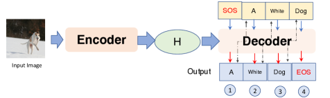
Figure 1: Working mechanism of neural image caption generator

Neural Image Caption Generation (NICG) [1, 9, 36, 37, 38, 6, 7, 22, 30] model calculates the conditional probability $P(Y|X)$, where $X$ is the input image and $Y=[y_{1},y_{2},\cdots,y_{n}]$ is the target token sequences that will be used as image captions. As shown in Fig. 1, the input image is first sent through the encoder $\mathcal{F}_{encoder}$ to produce the hidden representation $H$. After that, starting with a special token (SOS), the decoder $\mathcal{F}_{decoder}$ uses $H$ in an iterative way for an auto-regressive generation of output tokens $Y$. The tokens are generated one by one until the process reaches the end of sequence (EOS) token or a pre-set maximum length. As the process is iterative, NICG models’ computational resources consumption is proportional to the length of generated output sequence. Therefore, a longer output sequence would make the model less efficient.

2.2 DNNs Efficiency

The accuracy and complexity of DNN models are positively correlated. Excellent model accuracy often implies a large number of neural layers and complex model construction, followed by huge inference-time computational cost and low efficiency. To reduce DNNs inference-time cost and faster the inference processes for real-time applications, many related works have been proposed. The related work can be divided into two types, The first type [21, 43] prunes DNN models offline by identifying and removing the unimportant/redundant neurons. The second type [39, 11, 8] reduces the number of computations online by dynamically skipping the unnecessary part of DNNs, known as input-adaptive techniques. Even though the input-adaptive techniques balance the model accuracy with computational costs, this balance is not robust. According to the recent studies [13, 20, 15, 14, 5], the input-adaptive DNN models are not robust against the adversarial attack, i.e., these techniques cannot lower computational costs under adversarial scenarios.

2.3 Adversarial Attacks

The adversarial example refers to an intentionally modified version of the benign example (e.g., adding perturbations). With the human-unnoticeable perturbations, the adversarial example could fool even the state-of-the-art DNNs [3, 2, 35]. Normally, adversarial examples can be generated by performing perturbation that follows adversarial gradients [27] or optimizes perturbation with given loss [4]. The perturbation will be constrained by magnitude, among which $L_{2}$-Norm and $L_{inf}$-Norm are the most commonly used ones [3, 27]. According to the difference of prior knowledge on the victim DNN model, the adversarial example generation techniques could be categorized into the white-box attack and black-box attack [10, 29, 24, 3, 23, 27, 4, 32].

3 Preliminary

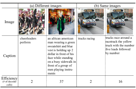
Figure 2: Efficiency uncertainty for images from MS-COCO

As we discussed in Sec. 2.1, NICG models will not terminate until the output token reaches EOS or a pre-set maximum length. In this section, we conduct a preliminary study to show that the value of the pre-set maximum length is hard to estimate because of the uncertainty in image caption tasks. Specifically, we select three images and corresponding captions from the MS-COCO dataset (shown in Fig. 2) to show the uncertainty.

Variance across Different Images. For different images, the task complexity of analyzing their contents could be completely different. In the image caption task, different image semantics will significantly affect NICG model efficiency. For example, in Fig. 2 (a), due to the difference in the scene semantics, the corresponding caption lengths of these two images have a huge difference.

Uncertainty in Labelling the Same Image. Another challenge to estimate max-length is the uncertainty from the training images. For example, in Fig. 2 (b), two different versions of the caption for the same training image have different lengths, which will increase the efficiency uncertainty in the NICG models trained with this image.

Because of the significant variance and uncertainty mentioned above, estimating an exact maximum length for each image is challenging. Thus, a common practice is to set a pretty large value for all images to avoid incomplete captioning (at least larger than the maximum caption length in the training dataset).

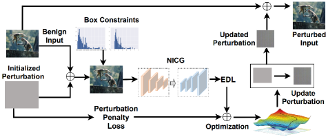
Figure 3: NICG workflow

4 Approach

4.1 Problem Formulation

$$\begin{split}&\quad\Delta=\text{argmax}_{\delta}\quad\text{Loop}_{\mathcal{F}}(x+\delta)\\ &s.t.\quad||\delta||\leq\epsilon\;\wedge\;||x+\delta||\in[0,1]^{n}\\ \end{split}$$ (1)

Our objective is to generate human-unnoticeable perturbations to images to decrease the victim NICG model efficiency during inference. Specifically, our objective concentrates on three factors: (i) the generated adversarial image should increase the victim NICG model computational complexity; (ii) the generated adversarial image $x^{\prime}$ can not be differentiated by humans from the benign image $x$; (iii) the generated adversarial image $x^{\prime}$ should be realistic in the real world. We formulate the mentioned three factors in Eq.(1). In Eq.(1), $x$ is the benign input, $\mathcal{F}$ is the victim NICG model under attack, $\epsilon$ is the maximum adversarial perturbation allowed, and $\text{Loop}_{\mathcal{F}}(\cdot)$ measures the number of decoder calls in the victim NICG model $\mathcal{F}$. Our proposed approach NICGSlowDown tries to search for an optimal perturbation $\Delta$ that maximizes the number of decoder calls while holding the constraints that perturbation is smaller than the allowed threshold (unnoticeable) and existing in the real world (realistic).

4.2 Attack Overview

Fig. 3 shows the overview of our proposed attack. Given a benign input image, NICGSlowDown first initializes an adversarial perturbation satisfying the realistic box constraints (§4.3.1). After that, NICGSlowDown computes the efficiency reduction loss (§4.3.2) and the perturbation penalty loss (§4.3.3). The reduction loss aims to slow down the victim NICG model, and the perturbation penalty loss seeks to enforce the generated adversarial examples to satisfy the unnoticeable constraints in Eq.(1). Finally, NICGSlowDown updates the adversarial perturbation by jointly optimizing the perturbation penalty loss and the efficiency reduction loss.

4.3 Detail Design

4.3.1 Realistic Box Constraints

$$\delta=\frac{1}{2}(tanh(w)+1)-x$$ (2)

To ensure the adversarial example is a valid image, we constraint the adversarial perturbation $\delta$ in Eq.(1): $||x+\delta||\in[0,1]^{n}$. Such constraints are known as box constraints in the optimization theory [3]. To satisfy the constraints, instead of directly optimizing $\delta$, we introduces a new variable $w$ and apply a change-of-variables to optimize over $w$. The relationship between $w$ and $\delta$ is shown in Eq.(2). Because the range of function $tanh(\cdot)$ is $[-1,1]$, $\delta+x$ will always satisfy the constraint $||x+\delta||\in[0,1]^{n}$.

4.3.2 Efficiency Reduction Loss

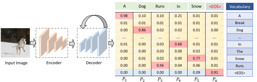
Figure 4: Distribution of output tokens

As we discussed in §Sec. 2.1, NICG model efficiency is related to the likelihood of the EOS tokens. Thus, to degrade the efficiency of NICG model, our intuition is to decrease the EOS tokens likelihood. Formally, let NICG model’s output be a sequence of probability distributions, i.e. $\mathcal{F}(x)=[p_{1},p_{2},\cdots,p_{n}]$ and the output token sequences are $[o_{1},o_{2},\cdots,o_{n}]$, where $o_{i}=\text{argmax}(p_{i})$. Then we denote the likelihood of the output tokens and the EOS tokens as $[p_{1}^{o_{1}},p_{2}^{o_{2}},\cdots,p_{n}^{o_{n}}]$ and $[p_{1}^{eos},p_{2}^{eos},\cdots,p_{n}^{eos}]$ respectively. In the example of Fig. 4, we have

$$\begin{split}[p_{1}^{o_{1}},p_{2}^{o_{2}},\cdots,p_{n}^{o_{n}}]=[0.98,0.86,0.56,0.68,0.77,0.91]\\ [p_{1}^{eos},p_{2}^{eos},\cdots,p_{n}^{eos}]=[0.00,0.00,0.00,0.00,0.09,0.91]\\ \end{split}$$

Then our efficiency reduction objective can be divided into two parts: (i) Delay EOS appearance and (ii) Break output dependency.

Minimize EOS Probability. To delay the appearance of EOS tokens, existing work usually applies minimum likelihood estimation (MLE) to minimize the likelihood of EOS tokens. However, as the NICG model vocabulary is normally pretty large (more than 1,000), MLE becomes inefficient because MLE requires to compute the cross-entropy loss, which is inefficient on large vocabulary. To address the limitation of inefficiency cross-entropy on large vocabulary, we borrow the idea of noise contrastive estimation (NCE) [12] and design our loss function. Specifically, we treat the probability distribution $p_{i}$ for the multi-classification task as a binary classification task i.e., is or not an EOS token. We then define a new probability distribution $q_{i}=[l_{i}^{eos},\sum_{j}l_{i}^{j}-l_{i}^{eos}]$ to represent the logits distribution of the proposed binary classification task. Finally, our goal to delay the appearance of the EOS token can be formulated as Eq.(3).

$$\mathcal{L}_{eos}=\frac{1}{n}\sum_{i=1}^{n}\left\{l_{i}^{eos}-\mathbb{E}_{k\sim p_{i}}l_{i}^{k}\right\}$$ (3)

With the help of logits $l_{i}^{j}$, we do not need to compute the softmax on large vocabulary thus could compute the objective function more efficiency. Next, we prove that our objective function Eq.(3) will convergence to MLE method’s loss function i.e., $L=\frac{1}{n}\sum_{i=1}^{n}\text{log}p_{i}^{eos}$ .

Lemma 1.

The proposed loss function $\mathcal{L}_{eos}$ will finally convergence to the MLE method’s objective function $L=\frac{1}{n}\sum_{i=1}^{n}\text{log}p_{i}^{eos}$.

Proof.

Denote the logits on the $i^{th}$ token as $[l_{i}^{1},l_{i}^{2},\cdots,l_{i}^{V}]$, where $V$ is the size of the vocabulary, then we have

$$p_{i}^{j}=\frac{\text{exp}(l_{i}^{j})}{\sum_{k=1}^{V}\text{exp}(l_{i}^{k})}$$

MSE seeks to minimize the likelihood of EOS, then the objective function is

$$L=\frac{1}{n}\sum_{i=1}^{n}\text{log}p_{i}^{eos}=\frac{1}{n}\sum_{i=1}^{n}\{l_{i}^{eos}-\text{log}\sum_{k=1}^{V}\text{exp}(l_{i}^{k})\}$$

the gradients of the above objective is

$$\frac{\partial L}{\partial x}=\frac{1}{n}\sum_{i=1}^{n}\left\{\frac{\partial l_{i}^{eos}}{\partial x}-\frac{\text{exp}(l_{i}^{k})}{\sum_{k=1}^{V}\text{exp}(l_{i}^{k})}\sum_{k=1}^{V}\frac{\partial l_{i}^{k}}{\partial x}\right\}$$

Notice that $p_{i}^{j}=\frac{\text{exp}(l_{i}^{j})}{\sum_{k=1}^{V}\text{exp}(l_{i}^{k})}$, then we have

$$\begin{split}&\frac{\partial L}{\partial x}=\frac{1}{n}\sum_{i=1}^{n}\left\{\frac{\partial l_{i}^{eos}}{\partial x}-\sum_{k=1}^{V}p_{i}^{k}\frac{\partial l_{i}^{k}}{\partial x}\right\}\\ &\quad\quad=\frac{1}{n}\sum_{i=1}^{n}\left\{\frac{\partial l_{i}^{eos}}{\partial x}-\mathbb{E}_{k\sim p_{i}}\frac{\partial l_{i}^{k}}{\partial x}\right\}\\ &\quad\quad=\frac{\partial\mathcal{L}_{eos}}{\partial x}\end{split}$$ (4)

∎

Because of the convergence of Monte Carlo method, we prove Lemma 1.

Break output Dependency. Because the token generation process of NICG models is a Markov process, i.e., NICG model outputs the probability distribution $p_{i}$ based on the previous output token $o_{i-1}$, i.e., $p_{i}=\mathcal{F}_{decoder}(o_{i-1},h)$. Minimize $p_{i}^{eos}$ may not change the output tokens at the positions from 0 to $n-1$. Thus minimizing $p_{n}^{eos}$ will be challenging because the previous token $o_{n-1}$ keeps the same. To accelerate the process of delaying EOS tokens, we seek to break such output dependency. Similar to the objective in delaying EOS appearance, we have the objective in Eq.(5).

$$\mathcal{L}_{dep}=\frac{1}{n}\sum_{i=1}^{n}\left\{l_{i}^{o_{i}}-\mathbb{E}_{k\sim p_{i}}l_{i}^{k}\right\}$$ (5)

Final Efficiency Reduction Objective. Our final efficiency reduction objective can be formulated as Eq.(6), which aims to delay the EOS token appearance and break the output dependency.

$$\mathcal{L}_{deg}=\mathcal{L}_{eos}+\lambda\mathcal{L}_{dep}$$ (6)

4.3.3 Perturbation Penalty Loss

$$\mathcal{L}_{per}=\left\{\begin{aligned} &\quad 0;\quad\quad\quad\text{if}\;\delta\leq\epsilon\\ &||\delta-\epsilon||;\quad\text{otherwise}\end{aligned}\right.$$ (7)

To ensure that the adversarial example will be unnoticeable to humans, we constraint the magnitude of the adversarial perturbation in Eq.(1), i.e., $||\delta||\leq\epsilon$. To achieve such goal, we introduce the perturbation penalty loss in Eq.(7), if the adversarial perturbation $\delta$ is less than the allowed perturbation magnitude, the penalty is zero, otherwise, the penalty will increase linearly as $||\delta-\epsilon||$ increases.

4.4 Attack Algorithm

Algorithm 1 NICGSlowDown Attack

Input: Benign input $x$
Input: Victim NICG model $\mathcal{F}(\cdot)$
Input: Maximum perturbation $\epsilon$
Input: Maximum Iterations T
Output: Adversarial examples $x^{\prime}$ that satisfy Eq.(1)

1:  $\delta\Leftarrow 0$       Initialize $\delta$ with 0.

2:  $w\Leftarrow arctanh(2x-1)$ Initialize $w$ based on Eq.(2).

3:  for $iter\;\text{in}\;\text{Range}$(T) do

4:     $x^{\prime}=\frac{1}{2}(tanh(w)+1)$ Compute $x^{\prime}$ based on Eq.(2)

5:     $\delta=x^{\prime}-x$  Compute the perturbation magnitude

6:     $\mathcal{L}_{deg}=L_{1}(x^{\prime},\mathcal{F})$ Compute $\mathcal{L}_{per}$ according to Eq.(6).

7:     $\mathcal{L}_{per}=L_{2}(\delta,\epsilon)$ Compute $\mathcal{L}_{per}$ according to Eq.(7).

8:     $\mathcal{L}_{total}=\mathcal{L}_{deg}+\lambda\mathcal{L}_{per}$ Compute joint loss.

9:     $\triangledown=\frac{\partial\mathcal{L}_{total}}{\partial w}$ Compute the gradients

10:     $w=w+lr\times\triangledown$ Update the latent variable $w$.

11:  end for

12:  Return $\frac{1}{2}(tanh(w)+1)$ Return the adversarial example.

The attack algorithm is shown in Algorithm 1. Our attack algorithm accepts four inputs: a benign input image $x$, the victim NICG model $\mathcal{F}$, a pre-defined perturbation threshold $\epsilon$, and the maximum iteration number T. Our algorithm outputs an adversarial example $x^{\prime}$ that satisfy Eq.(1). Our algorithm first initializes the adversarial perturbation $\delta$ as zero and compute the corresponding $w$ (line 1 and 2). After that, we iteratively update the latent variable $w$. Specifically, we compute the efficiency reduction loss $\mathcal{L}_{deg}$ based on Eq.(6) and the perturbation penalty loss based on Eq.(7). We then optimize $w$ by minimizing the joint losses. After iteration, we transform the latent variable $w$ back to image space and return the adversarial example.

5 Evaluation

5.1 Experimental Setup

Table 1: Experimental Subjects

Dataset	Subject	Model		Train	Valid	Test
		Encoder	Decoder
Flickr8k	A	ResNext	Attention + LSTM	6000	1000	1000
	B	GoogLeNet	Attention + RNN	6000	1000	1000
MS-COCO	C	MobileNets	Attention + LSTM	82783	40504	40775
	D	ResNet	Attention + RNN	82783	40504	40775

Models and Datasets. We evaluate our proposed technique  on two public datasets, Flickr8k [19], and MS-COCO [25]. Table 1 shows the detail of NICG models for each corresponding dataset. Flickr8k dataset contains 8,000 images (including 6,000 training images, 1,000 validation images and 1,000 test images). We apply two encoder-decoder models for the Flickr8k dataset. The first one applies ResNext [40] as encoder and LSTM module as decoder [18]. The second one applies GoogLeNet [34] as encoder and RNN as decoder [33]. MS-COCO dataset contains 123,287 images (including 82,783 training images, 40,504 validation images and 40,775 testing images). We also apply two encoder-decoder models for the MS-COCO dataset. The first one is MobileNets [21] + LSTM and the latter one is ResNet [16] + RNN.

$$\begin{split}&\quad\quad\text{I-Loop}=\frac{\text{Loop}(x^{\prime})-\text{Loop}(x)}{\text{Loop}(x)}\times 100\%\\ &\text{I-Latency}=\frac{\text{Latency}(x^{\prime})-\text{Latency}(x)}{\text{Latency}(x)}\times 100\%\\ \end{split}$$ (8)

Metrics. We select two metrics, the number of decoder calls and response latency, to represent the efficiency of NICG models. As we discussed in §2.1, higher decoder calls indicate that the NICG model cast more floating-point operations (FLOPs) to handle the input image, which leads to less efficiency [43, 39]. Response latency is a hardware-dependent metric used to measure NICG model runtime efficiency. High response latency indicates worse real-time caption quality and higher battery consumption. We measure the response latency on two hardware platforms: Intel Xeon E5-2660v3 CPU and Nvidia1080Ti GPU. Specifically, we define two metrics, I-Loop and I-Latency, to show the effectiveness of NICGSlowDown in degrading the NICG model efficiency. The formal definition of I-Loop and I-Latency are shown in (8), where $x$ and $x^{\prime}$ denotes the benign example and the generated adversarial example respectively, Loop($\cdot$) and Latency($\cdot$) are the functions to calculate the decoder calls and response latency respectively. Higher I-Loop and I-Latency refer to more severe efficiency slowdown caused by the adversarial example.

Comparison Baselines. To the best of our knowledge, we are the first to study the efficiency robustness of NICG models; therefore, no existing efficiency attacks can be applied as our baselines. To show that existing accuracy-based methods can not be applied to evaluate the NICG model’s efficiency robustness, we compare NICGSlowDown against two accuracy-based attack algorithms and four natural image corruptions. Specifically, we choose PGD [28] and CW [3]) as the accuracy-based attack algorithms and image quantization [42, 17], Gaussian noise [42, 17], JPEG compression [26] and feature squeezing [42] as the corruptions.

Implementation Details. We follow [41] to implement the four neural image caption generation models. We set the NICG model’s maximum caption length as 60 as the maximum caption length in the training dataset is 53. We filter out the tokens with frequencies less than 5. Finally, our vocabulary sizes are 2,633 and 11,569 for Flick8k and MS-COCO datasets. We implement NICGSlowDown with Pytorch and set the maximum perturbation $\epsilon$ as 40 and 0.03 for $L_{2}$ and $L_{inf}$ adversarial examples. We set maximum iteration $T$ as 1,000 and the hyper-parameter $\lambda$ as $1.0\times 10^{4}$.

5.2 Effectiveness and Severity

Effectiveness of Attack. Fig. 5 shows the distribution of efficiency metrics for Subject A (more results are shown in Appendix). The first and second rows represent the Probability Density Function (PDF) and Cumulative Distribution Function (CDF) results. For convenience, we reverse the CDF from one to zero. The area under the CDF curve indicates the efficiency of the NICG model, and a larger area indicates the NICG model is less efficient. The green area denotes the distribution of benign examples, and the red represents the distribution of adversarial examples generated by NICGSlowDown. From Fig. 5, we could observe that adversarial examples significantly change the number of decoder calls and latency distribution in the NICG model. This observation indicates that our attack could effectively slow down the NICG model.

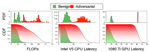
Figure 5: Efficiency distribution of benign and adversarial examples (More results can be found in appendix)

Table 2: Resutls of efficiency reduction

Subject	Norm	Metric	PGD	CW	Quantize	Gaussian	JPEG	TVM	Ours
A		I-Loop	87.30	7.26	3.97	0.47	-5.25	-0.12	483.86
	L2	I-Latency(CPU)	36.33	2.59	3.00	1.44	-3.28	-1.51	198.76
		I-Latency(GPU)	75.47	18.93	11.81	13.35	8.47	15.60	290.40
		I-Loop	7.42	44.88	6.37	0.79	-5.25	-0.12	354.11
	Linf	I-Latency(CPU)	3.86	16.68	2.43	1.82	-15.45	9.06	202.81
		I-Latency(GPU)	34.62	38.18	18.96	10.14	14.75	21.64	241.90
B		I-Loop	18.62	6.66	11.94	5.40	2.14	0.45	481.32
	L2	I-Latency(CPU)	2.77	3.73	24.65	-14.78	1.65	5.80	87.37
		I-Latency(GPU)	26.16	15.31	14.55	1.65	2.47	6.12	223.38
		I-Loop	8.22	36.74	10.33	0.04	2.14	0.45	271.19
	Linf	I-Latency(CPU)	1.86	6.32	-0.74	3.28	2.55	2.53	8.32
		I-Latency(GPU)	6.94	20.99	22.55	12.56	3.20	14.11	71.77
C		I-Loop	48.48	2.76	-0.08	7.96	-5.69	-0.96	433.58
	L2	I-Latency(CPU)	33.07	3.94	-0.17	3.32	-2.19	-11.01	155.61
		I-Latency(GPU)	32.14	14.51	13.75	19.19	2.34	9.98	297.37
		I-Loop	-5.97	62.89	3.49	-2.32	-5.69	-0.96	379.81
	Linf	I-Latency(CPU)	-9.33	20.48	1.54	-1.21	-3.60	8.19	90.73
		I-Latency(GPU)	6.23	29.24	16.97	13.08	20.19	21.06	211.41
D		I-Loop	19.07	11.17	-7.33	0.24	-3.53	0.17	408.90
	L2	I-Latency(CPU)	8.14	7.07	-4.62	-1.97	3.26	-2.45	155.49
		I-Latency(GPU)	31.95	17.32	8.08	31.16	21.59	15.87	192.58
		I-Loop	7.82	74.09	-8.35	1.51	-3.53	0.17	115.02
	Linf	I-Latency(CPU)	-1.13	29.04	-4.17	2.53	-3.53	-3.16	21.45
		I-Latency(GPU)	23.29	43.41	10.27	3.25	3.85	7.63	55.36

Impact of Attack. To evaluate the severity of our proposed attack on reducing the model efficiency, we measure the I-LOOP and I-Latency for the four subjects we mentioned above. Table 2 shows the results of the adversarial attack on the targeted model. From the table, we could have the following observations: (i) Compared to other baselines, NICGSlowDown achieves the best performance on slowing down the targeted NICG model in all subjects. For example, adversarial examples generated by NICGSlowDown increase the number of decoder calls, CPU latency, and GPU latency on Subject A up to 483.86%, 198.76%, 290.40% respectively; (ii) Unlike NICGSlowDown, all baseline methods can not ensure degrading efficiency of the NICG model. In some cases, baselines would even speed up the NICG model processing instead. This observation proves that the existing baseline techniques are not suitable for evaluating the efficiency robustness of NICG models; (iii) For all subjects, NICGSlowDown with L2-Norm achieves better performance compared with Linf-Norm. We infer that because the perturbation size of L2-Norm is more suitable for NICGSlowDown to apply efficiency attack; (iv) For all subjects, the GPU latency increased by NICGSlowDown is more effective than the CPU delay, implying that NICGSlowDown is more effective for efficiency attacks on GPU than CPU.

5.3 Quality of Generated Images

Table 3: The size of the adversarial perturbations

Norm	Approach	A	B	C	D	Avg
$L_{2}$	PGD	39.98	39.98	39.98	39.98	39.98
	CW	0.04	0.04	0.04	0.04	0.04
	Quantize	160.19	160.22	161.76	161.78	160.99
	Gaussian	38.25	38.25	38.08	38.08	38.16
	JPEG	160.85	160.85	161.06	161.06	160.96
	TVM	0.52	0.52	0.51	0.51	0.51
	Ours	4.25	4.30	4.82	5.18	4.64
$L_{inf}$	PGD	0.03	0.03	0.03	0.03	0.03
	CW	0.04	0.04	0.04	0.04	0.04
	Quantize	0.98	0.98	0.99	0.99	0.98
	Gaussian	0.03	0.03	0.03	0.03	0.03
	JPEG	0.92	0.92	0.93	0.93	0.93
	TVM	0.00	0.00	0.00	0.00	0.00
	Ours	0.04	0.04	0.04	0.02	0.04

5.3.1 Quantitative Evaluation

In this section, we measure the sizes of the generated adversarial examples. The results are shown in Table 3. The results show that NICGSlowDown generates adversarial examples with minimal perturbation sizes. Specifically, NICGSlowDown generates adversarial examples with the average perturbation size 4.64 for $L_{2}$ norm and 0.04 for $L_{inf}$ norm. The results imply NICGSlowDown generates adversarial examples that are unnoticeable to humans. Some baselines also generate adversarial examples with imperceptible perturbations, but they cannot affect the NICG model efficiency as expected, making the “unnoticeable” meaningless.

5.3.2 Qualitative Evaluation

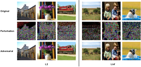
Figure 6: The generated adversarial examples

In this section, we discuss the quality of the generated adversarial inputs based on human perception. For that purpose, we randomly select six adversarial images and show the selected images in Fig. 6 (all generated adversarial images can be found on our website). The first column shows the benign images, the second column shows the adversarial perturbations used against each benign image, and the third column shows the resultant adversarial images. From the results in the first and the third rows, we observe that the added perturbation is not perceptible to humans.

5.4 More Studies

5.4.1 Accuracy VS. Efficiency

In this section, we evaluate the relationship between accuracy attack and efficiency attack. The results in Table 2 show that accuracy-based adversarial examples may not affect NICG model efficiency. In this section, we evaluate whether efficiency-based adversarial examples will affect NICG model accuracy. Specifically, we measure the BLEU scores [31] of the adversarial examples and the benign examples. Table 4 shows the BLEU scores of benign examples and adversarial examples generated by NICGSlowDown. From the results, we can observe that our attack significantly reduces the accuracy of the victim NICG model, decreasing the BLEU scores up to 100%. This observation indicates that the accuracy-based attack can impact only the NICG model accuracy without reducing efficiency. In contrast, our efficiency-based attack, NICGSlowDown, can effectively reduce the model efficiency and significantly lower the accuracy.

Table 4: BLEU scores of benign and adversarial examples

Subjects		benign	adversarial	decreasae
A	L2	0.17	0.00	100.00
	Linf	0.17	0.01	93.08
B	L2	0.20	0.00	99.02
	Linf	0.20	0.02	90.94
C	L2	0.10	0.00	98.77
	Linf	0.10	0.01	90.95
D	L2	0.11	0.01	91.43
	Linf	0.11	0.03	69.15

5.4.2 Hyper-Parameter Sensitively

In this section, we evaluate the effectiveness of the adversarial examples under different hyper-parameter settings. Specifically, we set the hyper-parameter $\lambda=[1.0\times 10^{3},1.0\times 10^{4},1.0\times 10^{5}]$ and run NICGSlowDown to generate adversarial examples. From the results in Table 5, we observe that the adversarial examples generated under different hyper-parameter settings show a stable performance, which implies NICGSlowDown is not sensitive to hyper-parameter settings.

Table 5: Effectiveness under different hyper-parameters

Subject ID	Norm	Metric	10	100	1000
A		I-Loop	483.86	483.86	483.86
	L2	I-Latency(CPU)	189.76	198.76	198.35
		I-Latency(GPU)	288.43	290.40	300.32
		I-Loop	360.21	354.11	344.11
	Linf	I-Latency(CPU)	190.32	202.81	190.43
		I-Latency(GPU)	250.32	241.90	227.32
B		I-Loop	479.32	481.32	481.32
	L2	I-Latency(CPU)	89.31	87.37	85.42
		I-Latency(GPU)	225.43	223.38	220.43
		I-Loop	283.24	271.19	271.19
	Linf	I-Latency(CPU)	10.21	8.32	8.11
		I-Latency(GPU)	75.43	71.77	69.31
C		I-Loop	435.56	433.58	433.58
	L2	I-Latency(CPU)	166.42	155.61	148.31
		I-Latency(GPU)	300.32	297.37	297.32
		I-Loop	388.31	379.81	370.54
	Linf	I-Latency(CPU)	91.31	90.73	89.31
		I-Latency(GPU)	222.32	211.41	210.32
D		I-Loop	410.23	408.90	408.90
	L2	I-Latency(CPU)	156.42	155.49	154.43
		I-Latency(GPU)	199.32	192.58	178.31
		I-Loop	117.23	115.02	113.13
	Linf	I-Latency(CPU)	22.12	21.45	18.23
		I-Latency(GPU)	56.43	55.36	50.13

6 Discussion

Application. Recently, NICG models have been widely deployed on resource-constrained devices; thus, the need for efficiency robustness evaluation is essential. For example, many mobile applications are developed to help visually impaired persons; most of those applications rely on the NICG model to provide image explanations to a person. In a situation like crossing a road, the response time should be minimum. Otherwise, fatal accidents can happen. Therefore, the evaluation of efficiency robustness is needed to avoid these scenarios.

Limitation. NICGSlowDown is a white-box approach, i.e., NICGSlowDown needs to access the victim NICG model parameters to generate adversarial examples. As we have not evaluated the transferability of the attack, we can not conclude that our attack can also be used in the black-box setting. However, as NICGSlowDown is designed for evaluating robustness instead of attacking, the white-box assumption is valid for NICGSlowDown. We leave the black-box evaluation for future work.

7 Conclusion

In this paper, our objective is to evaluate the efficiency robustness of NICG models. For this purpose, we propose NICGSlowDown that generates adversarial efficiency decreasing inputs explores a potential vulnerability of NICG models, i.e., the efficiency of NICG models is inversely proportional to the length of NICG output sequences. Based on the extensive evaluation, we can notice that NICGSlowDown can generate inputs that significantly decrease NICG models’ efficiency. To the best of our knowledge, this is the first adversarial attack exploring the efficiency robustness of NICG models.

Appendix

Appendix A More Evaluation Results

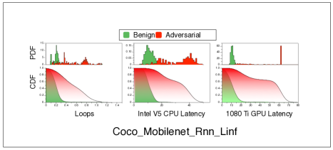
Figure 7: Efficiency Distribution

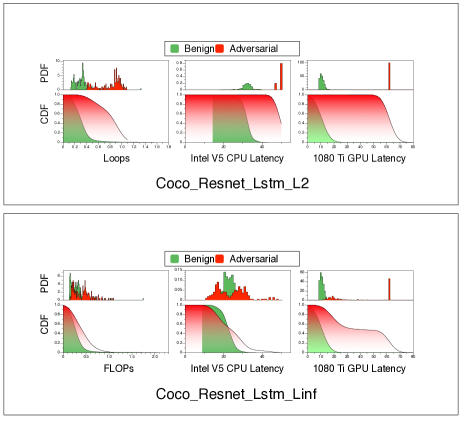
Figure 8: Efficiency Distribution

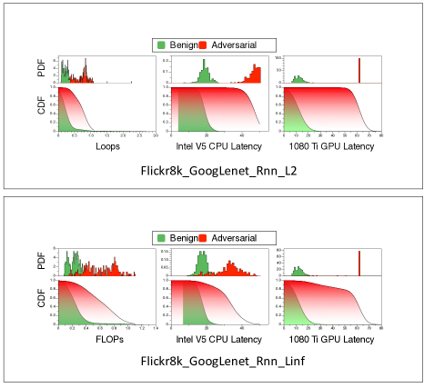
Figure 9: Efficiency Distribution

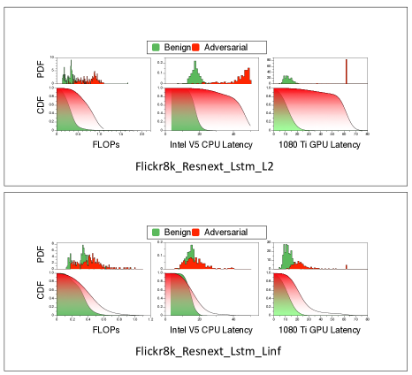
Figure 10: Efficiency Distribution

Figure 7, 8, 9, 10 show the efficiency distribution of benign images and the generated adversarial images.

The first and second rows represent the Probability Density Function (PDF) and Cumulative Distribution Function (CDF) results respectively. The area under the CDF curve indicates the efficiency of the NICG model, a larger area indicates the NICG model is less efficiency. The green area denotes the distribution of benign examples, and the red areas represent the distribution of adversarial examples generated by NICGSlowDown. From the results, we could observe that adversarial examples extremely change the FLOPs and latency distribution of NICG model. This observation is consistent with the results in Fig. 5.

Appendix B More Adversarial Examples

Fig. 11 shows more generated adversarial examples, we provide more adversarial examples on the zip files.

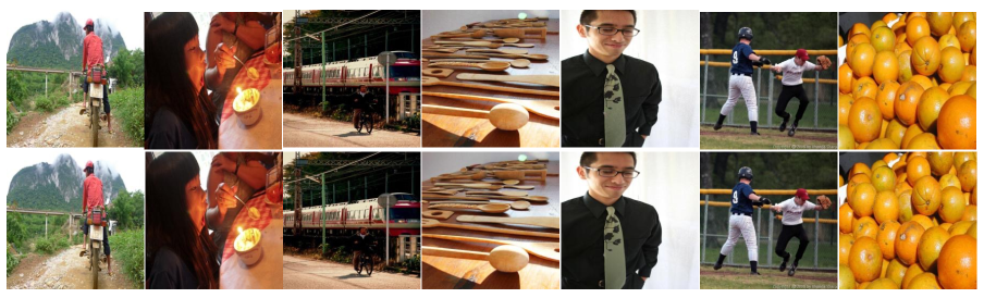
Figure 11: Generated adversarial examples

References

- [1] Peter Anderson, Xiaodong He, Chris Buehler, Damien Teney, Mark Johnson, Stephen Gould, and Lei Zhang. Bottom-Up and Top-down Attention for Image Captioning and Visual Question Answering. In 2018 IEEE Conference on Computer Vision and Pattern Recognition, CVPR 2018, Salt Lake City, UT, USA, June 18-22, 2018, pages 6077–6086, 2018.
- [2] Anish Athalye, Nicholas Carlini, and David A. Wagner. Obfuscated Gradients Give a False Sense of Security: Circumventing Defenses to Adversarial Examples. In Proceedings of the 35th International Conference on Machine Learning, ICML 2018, Stockholmsmässan, Stockholm, Sweden, July 10-15, 2018, pages 274–283, 2018.
- [3] Nicholas Carlini and David A. Wagner. Towards Evaluating the Robustness of Neural Networks. In 2017 IEEE Symposium on Security and Privacy, SP 2017, San Jose, CA, USA, May 22-26, 2017, pages 39–57, 2017.
- [4] Pin-Yu Chen, Yash Sharma, Huan Zhang, Jinfeng Yi, and Cho-Jui Hsieh. EAD: Elastic-net Attacks to Deep Neural Networks via Adversarial Examples. In Proceedings of the Thirty-Second AAAI Conference on Artificial Intelligence, (AAAI-18), the 30th innovative Applications of Artificial Intelligence (IAAI-18), and the 8th AAAI Symposium on Educational Advances in Artificial Intelligence (EAAI-18), New Orleans, Louisiana, USA, February 2-7, 2018, pages 10–17, 2018.
- [5] Simin Chen, Mirazul Haque, Zihe Song, Cong Liu, and Wei Yang. Transslowdown: Efficiency Attacks on Neural Machine Translation Systems. CoRR, 2021.
- [6] Riccardo Del Chiaro, Bartlomiej Twardowski, Andrew D. Bagdanov, and Joost van de Weijer. RATT: Recurrent Attention to Transient Tasks for Continual Image Captioning. In Advances in Neural Information Processing Systems 33: Annual Conference on Neural Information Processing Systems 2020, NeurIPS 2020, December 6-12, 2020, virtual, pages 16736–16748, 2020.
- [7] Marcella Cornia, Matteo Stefanini, Lorenzo Baraldi, and Rita Cucchiara. Meshed-memory Transformer for Image Captioning. In 2020 IEEE/CVF Conference on Computer Vision and Pattern Recognition, CVPR 2020, Seattle, WA, USA, June 13-19, 2020, pages 10575–10584, 2020.
- [8] Michael Figurnov, Maxwell D. Collins, Yukun Zhu, Li Zhang, Jonathan Huang, Dmitry P. Vetrov, and Ruslan Salakhutdinov. Spatially Adaptive Computation Time for Residual Networks. In 2017 IEEE Conference on Computer Vision and Pattern Recognition, CVPR 2017, Honolulu, HI, USA, July 21-26, 2017, pages 1790–1799, 2017.
- [9] Zhe Gan, Chuang Gan, Xiaodong He, Yunchen Pu, Kenneth Tran, Jianfeng Gao, Lawrence Carin, and Li Deng. Semantic Compositional Networks for Visual Captioning. In 2017 IEEE Conference on Computer Vision and Pattern Recognition, CVPR 2017, Honolulu, HI, USA, July 21-26, 2017, pages 1141–1150, 2017.
- [10] Ian J. Goodfellow, Jonathon Shlens, and Christian Szegedy. Explaining and Harnessing Adversarial Examples. In 3rd International Conference on Learning Representations, ICLR 2015, San Diego, CA, USA, May 7-9, 2015, Conference Track Proceedings, 2015.
- [11] Alex Graves. Adaptive Computation Time for Recurrent Neural Networks. CoRR, abs/1603.08983, 2016.
- [12] Michael Gutmann and Aapo Hyvärinen. Noise-contrastive Estimation: A New Estimation Principle for Unnormalized Statistical Models. In Proceedings of the thirteenth international conference on artificial intelligence and statistics, pages 297–304, 2010.
- [13] Mirazul Haque, Anki Chauhan, Cong Liu, and Wei Yang. ILFO: Adversarial Attack on Adaptive Neural Networks. In 2020 IEEE/CVF Conference on Computer Vision and Pattern Recognition, CVPR 2020, Seattle, WA, USA, June 13-19, 2020, pages 14252–14261, 2020.
- [14] Mirazul Haque, Simin Chen, Wasif Arman Haque, Cong Liu, and Wei Yang. NODEattack: Adversarial Attack on the Energy Consumption of Neural Odes. CoRR, 2021.
- [15] Mirazul Haque, Yaswanth Yadlapalli, Wei Yang, and Cong Liu. EREBA: Black-box Energy Testing of Adaptive Neural Networks. In 2022 IEEE/ACM 43rd International Conference on Software Engineering (ICSE), 2022.
- [16] Kaiming He, Xiangyu Zhang, Shaoqing Ren, and Jian Sun. Deep Residual Learning for Image Recognition. In 2016 IEEE Conference on Computer Vision and Pattern Recognition, CVPR 2016, Las Vegas, NV, USA, June 27-30, 2016, pages 770–778, 2016.
- [17] Dan Hendrycks and Thomas G. Dietterich. Benchmarking Neural Network Robustness to Common Corruptions and Perturbations. In 7th International Conference on Learning Representations, ICLR 2019, New Orleans, LA, USA, May 6-9, 2019, 2019.
- [18] Sepp Hochreiter and Jürgen Schmidhuber. Long Short-Term Memory. Neural Comput., 9:1735–1780, 1997.
- [19] Micah Hodosh, Peter Young, and Julia Hockenmaier. Flickr8k Dataset.
- [20] Sanghyun Hong, Yigitcan Kaya, Ionut-Vlad Modoranu, and Tudor Dumitras. A Panda? No, It’s a Sloth: Slowdown Attacks on Adaptive Multi-exit neural network inference. In 9th International Conference on Learning Representations, ICLR 2021, Virtual Event, Austria, May 3-7, 2021, 2021.
- [21] Andrew G. Howard, Menglong Zhu, Bo Chen, Dmitry Kalenichenko, Weijun Wang, Tobias Weyand, Marco Andreetto, and Hartwig Adam. Mobilenets: Efficient Convolutional Neural Networks for Mobile Vision applications. CoRR, abs/1704.04861, 2017.
- [22] Lun Huang, Wenmin Wang, Jie Chen, and Xiaoyong Wei. Attention on Attention for Image Captioning. In 2019 IEEE/CVF International Conference on Computer Vision, ICCV 2019, Seoul, Korea (South), October 27 - November 2, 2019, pages 4633–4642, 2019.
- [23] Uyeong Jang, Xi Wu, and Somesh Jha. Objective Metrics and Gradient Descent Algorithms for Adversarial Examples in Machine Learning. In Proceedings of the 33rd Annual Computer Security Applications Conference, Orlando, FL, USA, December 4-8, 2017, pages 262–277, 2017.
- [24] Alexey Kurakin, Ian J. Goodfellow, and Samy Bengio. Adversarial Examples in the Physical World. In 5th International Conference on Learning Representations, ICLR 2017, Toulon, France, April 24-26, 2017, Workshop Track Proceedings, 2017.
- [25] Tsung-Yi Lin, Michael Maire, Serge Belongie, James Hays, Pietro Perona, Deva Ramanan, Piotr Dollár, and C Lawrence Zitnick. Microsoft COCO: Common Objects in Context. In European Conference on Computer Vision, pages 740–755, 2014.
- [26] Zihao Liu, Qi Liu, Tao Liu, Nuo Xu, Xue Lin, Yanzhi Wang, and Wujie Wen. Feature Distillation: Dnn-oriented JPEG Compression against Adversarial Examples. In 2019 IEEE/CVF Conference on Computer Vision and Pattern Recognition (CVPR), pages 860–868, 2019.
- [27] Aleksander Madry, Aleksandar Makelov, Ludwig Schmidt, Dimitris Tsipras, and Adrian Vladu. Towards Deep Learning Models Resistant to Adversarial Attacks. In 6th International Conference on Learning Representations, ICLR 2018, Vancouver, BC, Canada, April 30 - May 3, 2018, Conference Track Proceedings, 2018.
- [28] Aleksander Madry, Aleksandar Makelov, Ludwig Schmidt, Dimitris Tsipras, and Adrian Vladu. Towards Deep Learning Models Resistant to Adversarial Attacks. In International Conference on Learning Representations, 2018.
- [29] Seyed-Mohsen Moosavi-Dezfooli, Alhussein Fawzi, and Pascal Frossard. Deepfool: A Simple and Accurate Method to Fool Deep Neural Networks. In 2016 IEEE Conference on Computer Vision and Pattern Recognition, CVPR 2016, Las Vegas, NV, USA, June 27-30, 2016, pages 2574–2582, 2016.
- [30] Yingwei Pan, Ting Yao, Yehao Li, and Tao Mei. X-Linear Attention Networks for Image Captioning. In 2020 IEEE/CVF Conference on Computer Vision and Pattern Recognition, CVPR 2020, Seattle, WA, USA, June 13-19, 2020, pages 10968–10977, 2020.
- [31] Kishore Papineni, Salim Roukos, Todd Ward, and Wei-Jing Zhu. BLEU: A Method for Automatic Evaluation of Machine Translation. In Proceedings of the 40th annual meeting of the Association for Computational Linguistics, pages 311–318, 2002.
- [32] Jérôme Rony, Luiz G. Hafemann, Luiz S. Oliveira, Ismail Ben Ayed, Robert Sabourin, and Eric Granger. Decoupling Direction and Norm for Efficient Gradient-Based L2 Adversarial Attacks and Defenses. In IEEE Conference on Computer Vision and Pattern Recognition, CVPR 2019, Long Beach, CA, USA, June 16-20, 2019, pages 4322–4330, 2019.
- [33] David E. Rumelhart, Geoffrey E. Hinton, and Ronald J. Williams. Learning Representations by Back-propagating Errors. Nature, 323:533–536, 1986.
- [34] Christian Szegedy, Wei Liu, Yangqing Jia, Pierre Sermanet, Scott E. Reed, Dragomir Anguelov, Dumitru Erhan, Vincent Vanhoucke, and Andrew Rabinovich. Going Deeper with Convolutions. In IEEE Conference on Computer Vision and Pattern Recognition, CVPR 2015, Boston, MA, USA, June 7-12, 2015, pages 1–9, 2015.
- [35] Christian Szegedy, Wojciech Zaremba, Ilya Sutskever, Joan Bruna, Dumitru Erhan, Ian J. Goodfellow, and Rob Fergus. Intriguing Properties of Neural Networks. In 2nd International Conference on Learning, 2014.
- [36] Ashish Vaswani, Noam Shazeer, Niki Parmar, Jakob Uszkoreit, Llion Jones, Aidan N. Gomez, Lukasz Kaiser, and Illia Polosukhin. Attention is All you Need. In Advances in Neural Information Processing Systems 30: Annual Conference on Neural Information Processing Systems 2017, December 4-9, 2017, Long Beach, CA, USA, pages 5998–6008, 2017.
- [37] Oriol Vinyals, Alexander Toshev, Samy Bengio, and Dumitru Erhan. Show and Tell: A Neural Image Caption Generator. In IEEE Conference on Computer Vision and Pattern Recognition, CVPR 2015, Boston, MA, USA, June 7-12, 2015, pages 3156–3164, 2015.
- [38] Jing Wang, Jinhui Tang, and Jiebo Luo. Multimodal Attention with Image Text Spatial Relationship for OCR-Based Image Captioning. In MM ’20: The 28th ACM International Conference on Multimedia, Virtual Event / Seattle, WA, USA, October 12-16, 2020, pages 4337–4345, 2020.
- [39] Xin Wang, Fisher Yu, Zi-Yi Dou, Trevor Darrell, and Joseph E. Gonzalez. SkipNet: Learning Dynamic Routing in Convolutional Networks. In Computer Vision - ECCV 2018 - 15th European Conference, Munich, Germany, September 8-14, 2018, Proceedings, Part XIII, volume 11217, pages 420–436, 2018.
- [40] Saining Xie, Ross B. Girshick, Piotr Dollár, Zhuowen Tu, and Kaiming He. Aggregated Residual Transformations for Deep Neural Networks. In 2017 IEEE Conference on Computer Vision and Pattern Recognition, CVPR 2017, Honolulu, HI, USA, July 21-26, 2017, pages 5987–5995, 2017.
- [41] Kelvin Xu, Jimmy Ba, Ryan Kiros, Kyunghyun Cho, Aaron Courville, Ruslan Salakhudinov, Rich Zemel, and Yoshua Bengio. Show, Attend and Tell: Neural Image Caption Generation with Visual Attention. In International conference on machine learning, pages 2048–2057, 2015.
- [42] Weilin Xu, David Evans, and Yanjun Qi. Feature Squeezing: Detecting Adversarial Examples in Deep Neural Networks. In 25th Annual Network and Distributed System Security Symposium, NDSS 2018, San Diego, California, USA, February 18-21, 2018, 2018.
- [43] Xiangyu Zhang, Xinyu Zhou, Mengxiao Lin, and Jian Sun. Shufflenet: An Extremely Efficient Convolutional Neural Network for Mobile Devices. In 2018 IEEE Conference on Computer Vision and Pattern Recognition, CVPR 2018, Salt Lake City, UT, USA, June 18-22, 2018, pages 6848–6856, 2018.