From ten-flavor tests of the $\beta$-function to $\alpha_{s}$ at the Z-pole

Abstract

New tests are applied to two $\beta$-functions of the much-discussed BSM model with ten massless fermion flavors in the fundamental representation of the SU(3) color gauge group. The renormalization scheme of the two $\beta$-functions is defined on the gauge field gradient flow in respective finite or infinite physical volumes at zero lattice spacing. Recently published results in the ten-flavor theory led to indicators of an infrared fixed point (IRFP) in the finite-volume step $\beta$-function in the strong coupling regime of the theory [1]. We analyze our substantially extended set of ten-flavor lattice ensembles at strong renormalized gauge couplings and find no evidence or hint for IRFP in the finite-volume step $\beta$-function within controlled lattice reach. We also discuss new ten-flavor tests of the recently introduced lattice definition and algorithmic implementation of the $\beta$-function defined on the gradient flow of the gauge field over infinite Euclidean space-time in the continuum. Originally we introduced this new algorithm to match finite-volume step $\beta$-functions in massless near-conformal gauge theories with the infinite-volume $\beta$-function reached in the chiral limit from small fermion mass deformations of spontaneous chiral symmetry breaking. Results from the lattice analysis of the ten-flavor infinite-volume $\beta$-function are consistent with the absence of IRFP from our step $\beta$-function based analysis. We make important contact at weak coupling in infinite volume with gradient flow based three-loop perturbation theory, serving as a first pilot study toward the long-term goal of developing alternate approach to the determination of the strong coupling $\alpha_{s}$ at the Z-boson pole in QCD. Without reporting here, our tests of this long-term goal continue in QCD with three massless fermion flavors and in the SU(3) Yang-Mills limit of quenched QCD.

1 Introduction and outline

We report new test results here for two complementary $\beta$-functions of the much-discussed BSM model with ten massless fermion flavors in the fundamental representation of the SU(3) color gauge group. Details of the tests are presented for the gauge field gradient flow based ten-flavor step $\beta$-function in finite volumes, complemented by shorter discussion of the recently introduced lattice based algorithm for the ten-flavor $\beta$-function over infinite four-dimensional Euclidean space-time. The ten-flavor model is particularly relevant for its known BSM popularity when analyzed as a mass-deformed conformal theory, built on the hypothesis of conformal IRFP in the massless fermion limit [2]. The analysis of the mass-deformed conformal ten-flavor theory would be different under the alternate hypothesis of mass-deformed near-conformal behavior from spontaneous chiral symmetry breaking without IRFP in the massless limit. The anticipation of conformal behavior with IRFP at strong coupling in the massless fermion limit of the ten-flavor theory has been motivated by published lattice analyses in [3, 4, 1]. In contrast, our previous results [5, 6] and the extended new analysis reported here do not show any hints or indicators of IRFP in the two $\beta$-functions of the model within controlled lattice reach of the strong coupling region.

We will compare our new analysis with results from [1] where the most recent systematic effort was presented on emergent IRFP in the theory. Earlier results in [3, 4] on the location of the ten-flavor IRFP in the $g^{2}\approx 6-8$ range were ruled out in [5, 6], in agreement with [1]. However, we differ with the analysis from [1] where indicators were presented for the shift of the IRFP to the $g^{2}\approx 11-12$ range. The authors in [1] are careful to interpret their lattice evidence for the emergent IRFP presenting it as a likely scenario with added cautious warning on the control of lattice effects. We will show in Section 2 that the likely source of the disagreement is the statistical analysis in [1] without noticing the unresolved ambiguity in extrapolating from small lattice volumes to the continuum limit using domain wall fermion (DWF) lattice implementation. We did not find indicators for IRFP in the theory from our own analysis of this ambiguity in fitting the published DWF data sets of [1]. This is consistent with our staggered fermion based analysis not supporting IRFP in significantly larger volumes than allowed by DWF based lattice resources.

We also discuss new ten-flavor tests of the recently introduced lattice definition and algorithmic implementation of the $\beta$-function defined on the gradient flow of the gauge field over infinite Euclidean space-time in the continuum. Originally we introduced this new algorithm to match finite-volume step $\beta$-functions in massless near-conformal gauge theories with the infinite-volume $\beta$-function in the chiral limit, reached from small fermion mass deformations of spontaneous chiral symmetry breaking [7]. New results from the lattice analysis of the ten-flavor infinite-volume $\beta$-function are consistent with the absence of IRFP from our finite-volume step $\beta$-function based analysis. We make important contact at weak coupling with infinite volume based three-loop perturbation theory using the renormalization scheme as defined by the gradient flow [8, 9, 10, 11]. This serves as a first pilot study toward the long-term goal of developing alternate approach to the determination of the strong coupling $\alpha_{s}$ at the Z-boson pole in QCD. Our tests of this long-term goal continue in QCD with three massless fermion flavors and in the SU(3) Yang-Mills limit of quenched QCD [12]. In Section 2 we present our new analysis of the finite physical volume based ten-flavor step $\beta$-function in the continuum limit. In Section 3 we report new test results on the infinite volume based ten-flavor $\beta$-function with conclusions.

2 New analysis of the finite-volume step $\beta$-function with ten flavors

2.1 Renormalization on the gauge field gradient flow

The gradient flow in field theory was originally introduced as a method to regularize divergences and ultraviolet fluctuations in lattice calculations [8, 13]. The gradient flow based diffusion of the gauge fields on lattice configurations from Hybrid Monte Carlo (HMC) simulations became the method of choice for studying renormalization effects with great accuracy on the lattice [8, 9, 10, 14, 15]. Scale setting in lattice QCD was the immediate first application [9, 16, 17] before it became an important nonperturbative tool to calculate $\beta$-functions and scale dependent running couplings in gauge theories with the scale set by the finite physical volume.

In particular, we introduced earlier the gradient flow based scale-dependent renormalized gauge coupling $g^{2}(L)$ where the scale is set by the linear size $L$ of the finite physical volume [18]. This implementation is based on the gauge invariant trace of the non-Abelian quadratic field strength, $E(t)=-\frac{1}{2}{\rm Tr}F_{\mu\nu}F_{\mu\nu}(t)$, renormalized as a composite operator at gradient flow time $t$ on the gauge configurations,

$$g^{2}(L)=\frac{128\pi^{2}\langle t^{2}E(t)\rangle}{3(N^{2}-1)(1+\delta(c))},\hskip 14.22636ptE(t)=-\frac{1}{2}{\rm Tr}~{}F_{\mu\nu}(t)F_{\mu\nu}(t),$$ (2.1)

where $t$ is the flow time parameter with SU(N) color group of the non-Abelian gauge field from discretized lattice implementation of the flow time evolution. The one-parameter finite-volume renormalization scheme and the related gradient flow time $t(L)$ are set by the choice $c=\sqrt{8t}/L$ in the $L^{4}$ physical volume and with $\delta(c)$ defined in terms of Jacobi elliptic functions in [18]. The definition is designed to match the gradient flow based gauge coupling with the $\overline{\rm MS}$ scheme at leading order $g^{2}(L)=g^{2}_{\overline{\rm MS}}$ for any chosen value of $c$ from this one-parameter family.

2.2 The ten-flavor lattice ensembles of our analysis

The renormalization schemes $c=0.25,$ $c=0.275$, and $c=0.30$, used in our work, are identical to the ones used in [1] including periodic boundary conditions on gauge fields and anti-periodic boundary conditions on fermion fields in all four directions of the lattice. A general method for the scale-dependent renormalized gauge coupling $g^{2}(L)$ was introduced earlier to probe the step $\beta$-function, defined as $(g^{2}(sL)-g^{2}(L))/\log(s^{2})$ for some preset finite scale change $s$ in the linear physical size $L$ of the four-dimensional volume in the continuum limit of lattice discretization [19]. To avoid any confusion, the sign convention of the lattice based step $\beta$-function is the opposite of the conventional off-lattice literature. We use step sizes $s=2,~{}s=3/2,~{}s=4/3$ in our analysis of the gradient flow based renormalization scheme. Restricted to limited volume sizes by the DWF implementation, only step size $s=2$ was analyzed in [1]. In our implementation of the step $\beta$-function analysis, staggered lattice fermions are used with stout smearing in the fermion Dirac operator. Large volumes in staggered fermion implementation lead to important cross-checks from multiple step choices of $s$.

The Markov Chain Monte Carlo (MCMC) based gauge field generation of the lattice ensembles use the Rational Hybrid Monte Carlo (RHMC) evolution code as described in [20] together with further details on the lattice implementation of the step $\beta$-function and its continuum limit. Similar but not identical procedures are followed here. We generated lattice ensembles with $L^{4}$ lattice volumes in the range $L=8,10,12,14,16,18,20,24,28,30,32,36,40,48$ at 21 bare gauge couplings $g_{0}^{2}$ with $6/g_{0}^{2}=2.6,2.7,2.8,2.9,3.0,$ $3.1,3.2,3.3,3.4,3.5,3.6,3.7,3.8,3.9,4.0,4.1,4.5,5.0,6.0,7.0,8.0.$ In the new infinite volume $\beta$-function analysis of Section 3 only the large volumes with $L=32,36,40,48$ were used. For comparison, in [1] lattice ensembles at 17 bare gauge couplings were analyzed with linear lattice sizes $L=8,10,12,14,16,20,24,28,32$ restricted by the cost of the DWF implementation for improved chiral fermion properties in comparison with staggered fermions we use in large volumes.

Implementing the gradient flow on the lattice requires the discretization of the action density $E=-\frac{1}{2}{\rm Tr}~{}F_{\mu\nu}F_{\mu\nu}$. This appears in three places: the weight in MCMC simulation, the flow of the gauge field, and the observable $\langle t^{2}E(t)\rangle$ at flow time $t$. Varying the discretization scheme is a critical test for controlled cutoff effects, as all discretization schemes must agree in the continuum limit. Our RHMC simulations use Symanzik-improved action and along the gradient flow independently both the Symanzik and Wilson gauge actions, and for the observable $\langle t^{2}E(t)\rangle$ both the clover and Symanzik versions are used. We do not use the Wilson plaquette action for the observable $\langle t^{2}E(t)\rangle$ with the clover operator showing improved cutoff effects [9]. This gives four combinations, e.g. $WSC$ for Wilson flow on Symanzik RHMC gauge configuration generation and with clover observable for the renormalized coupling. The other three schemes $SSC$, $SSS$, and $WSS$ are designated accordingly. Consistency for results from these scheme on the gradient flow were tested with results presented in what follows.

Each of the four schemes can be implemented with their original lattice definition (unimproved), or with tree-level improvement to reduce cutoff effects. We introduced the method of tree-level improvement for the gradient flow earlier [21]. These improvements are expected to be most effective at weak couplings. Since tree-level improvements only effect the gauge field flow, it is expected to work best in perturbation theory when the one-loop $\beta$-function dominates. Large fermion loop contributions, which would be improved only in next order beyond tree-level, will begin to dominate for large flavor numbers, like the model here with nf=10. The large influence of fermion dynamics drives the nf=10 theory toward the conformal window. Tree-level improved operators are more ad hoc modifications at strong coupling and it is difficult to predict their cutoff-reducing effects. Their deployment requires care because in some cases it can lead to counter-intuitive effects. We tested tree-level improvement of the four schemes on the gradient flow at every targeted coupling $g^{2}$ for both $\beta$-functions with consistent results, not all of it shown below in limited space.

2.3 Analysis of the finite volume based step $\beta$-function at c=0.25

We applied the same algorithmic procedure as in [1] to compare results. At fixed $L$, we measure the renormalized gauge coupling $g^{2}$ on the gradient flow at each bare gauge coupling $g_{0}^{2}$ appearing in the $6/g_{0}^{2}$ form in the lattice gauge action. The flow time is set by the choice $c=0.25$ in the procedure. For a given choice of the scaled step, like $s=2$, or $s=3/2$, we pair $L$ and $sL$ lattices giving lattice step functions $(g^{2}(sL)-g^{2}(L))/{\rm log}(s^{2})$ at each bare lattice gauge coupling, with $g^{2}$ measured for a given $L$ on the gradient flow at $c=0.25$ for each $g_{0}^{2}$. In the next step we target preselected $g^{2}$ values, held to be identical for all $L$-pairs to be able to take the continuum limit $a^{2}/L^{2}\rightarrow 0$ at each targeted renormalized coupling $g^{2}$. One way to implement this synchronization is to fit a 4th order polynomial first with good statistical confidence at each L to $(g^{2}(sL)-g^{2}(L))/{\rm log}(s^{2})$ as a function of $g^{2}$ measured at 21 bare gauge couplings for fixed $L$. Using standard interpolations procedure from the polynomial fits, we calculate the lattice step $\beta$-functions $(g^{2}(sL)-g^{2}(L))/{\rm log}(s^{2})$ at any given $L$-pair for each of the targeted $g^{2}$ values. The targeted $g^{2}$-sequence seems to be arbitrary but it is simply designed to sample the continuous range of $g^{2}(L)$ where the lattice spacing can be removed safely, based on fits to data from the selected lattice ensembles. Every preselected $g^{2}$ implicitly defines a physical scale $L$ in the continuum. For illustration we show these fits and interpolations at $c=0.25$ in Fig. A.1 of the Appendix for lattice step functions $(g^{2}(sL)-g^{2}(L))/{\rm log}(s^{2})$ with and without tree-level improvement for the $L=24\rightarrow L=48$ pair with steps $s=2,s=3/2,s=4/3$. For each $L$-pair we have 24 combinations of the $SSC,SSS,WSC,WSS$ schemes with three step choices of $s$, unimproved, or improved. We have eight $L$-pairs with 24 fits each for the lattice ensembles listed above. Red circles mark the lattice step $\beta$-functions at targeted $g^{2}$ locations in the unimproved schemes and cyan circles show the analysis with tree-level improvement in Fig. A.1. Similar procedures are followed for $c=0.275$ and $c=0.30$ with $c=0.30$ shown in Fig. A.2.

In the last step of the fitting procedure the interpolated lattice step $\beta$-functions, $(g^{2}(sL)-g^{2}(L))/{\rm log}(s^{2})$, at all targeted $g^{2}$ values are extrapolated to the $a^{2}/L^{2}\rightarrow 0$ continuum limit. Typically six or seven pairs were used with linear or quadratic fits in $a^{2}/L^{2}$ at step $s=2$ and four or five pairs at $s=3/2$ and $s=4/3$. The linear and quadratic fits in $a^{2}/L^{2}$ were accepted if they produced statistically consistent results.

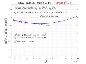
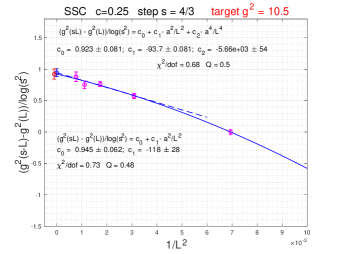
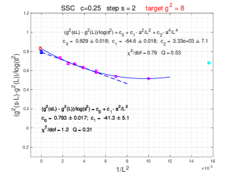
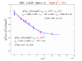
Figure 1: For $g^{2}=8$ in the continuum limit, the upper left panel shows linear fit in $a^{2}/L^{2}$ with lower L-values of the pairs at $L=18,24,30,36$ for step $s=4/3$ and quadratic fit when the $L=12\rightarrow 16$ pair is added to the fit. The upper right panel shows similar fits when $g^{2}=10.5$. The two lower panels are fits at $s=2$. The Q-values of the fits are discussed as P-value hypothesis tests in the notation of [1].

Fig. 1 shows fits in the $SSC$ scheme at targeted couplings $g^{2}=8$ and $g^{2}=10.5$ with scaled step sizes $s=4/3$ and $s=2$ and with statistical consistency between linear and quadratic fitting in $a^{2}/L^{2}$ for extrapolation to the continuum limit. The consistency of the continuum limit with linear and quadratic fitting in the $g^{2}=8-10.5$ range is particularly important in comparison with the $c=0.25$ analysis of [1] in the same range, as further discussed below.

Moving now to the targeted continuous $g^{2}$ range where continuum limits can be taken with statistical consistency, in Fig. 2 we show fitted results of the continuum step $\beta$-function, $(g^{2}(sL)-g^{2}(L))/{\rm log}(s^{2})$. Sampling from the continuous (color-shaded) range of $g^{2}$ values are shown with fits in the $\chi^{2}/dof\approx 1$ range. The size of the finite physical volume in the continuum limit is implicitly set by the value of $g^{2}(L)$ which is held fixed for all $L$-pairs while the cutoff is being removed.

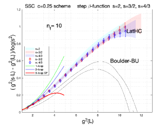
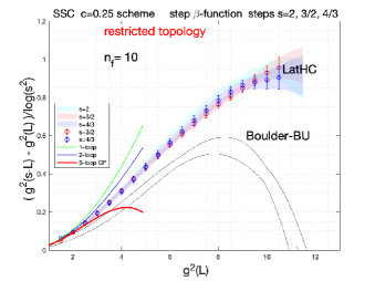
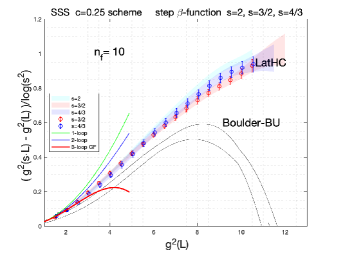
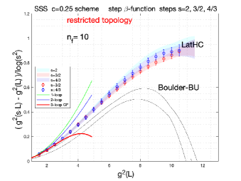
Figure 2: Fits of our data sets without tree-improvement are marked with LatHC tag in the plots and fit results from the authors of [1] are marked with Boulder-BU tag. We will keep these tags in several plots of the report. The upper left panel shows LatHC fit results for the continuum step $\beta$-function, $(g^{2}(sL)-g^{2}(L))/{\rm log}(s^{2})$, in the $SSC$ scheme at three different step sizes in the $g^{2}=1.5-12$ range of the continuum theory. The $s=2$ fits were quadratic in $a^{2}/L^{2}$, the $s=3/2$ and $s=4/3$ fits were linear in $a^{2}/L^{2}$. Two black lines represent the upper and lower errors of the band from [1] in the tree-level improved nWSS scheme of the paper. The upper right panel shows the same fitting procedure for gauge configurations with the topological charge restricted to the $Q_{\rm top}\leq 0.3$ range without any significant effect, as discussed in the text. The two lower panels show the tests for the $SSS$ scheme with the same fitting procedure as the $SSC$ scheme.

The incompatible results in Fig. 2 are striking with overwhelming statistical significance between the LatHC-tagged analysis with monotonic step $\beta$-function and the BoulderBU-tagged analysis of [1] hitting an IRFP around $g^{2}\approx 11$. We will identify the most likely source of this discrepancy in what follows below. Cutoff effects from topological charge fluctuations do not explain the discrepancy. On the two right-side panels of Fig. 2 we show that restricting the topological charge in the LatHC fits to the $Q_{\rm top}\leq 0.3$ range has no significant effect. We only did this in response to [1] where the issue was raised, although with small effects found in the DWF based analysis as well. We do not see any justification for imposing topological charge based cuts on the analysis with added remark in Section 2.5 on the Dirac spectrum of staggered lattice fermions.

There are two added features of the LatHC fits in Fig. 2. With $SSC$ and $SSS$ fits shown, consistency is as expected at fixed choices of $c$ and $s$ across different schemes on the gradient flow leading to the same continuum step $\beta$-function. We also find similar consistency fitting the $WSC$ and $WSS$ schemes. The three step sizes with $s=2,3/2,4/3$ will have slightly different shapes which we cannot resolve with the limited accuracy of our data. They all would be calculable from the $s\rightarrow 1$ limit of the finite-volume step function and they all should flow into the same IRFP in the $c=0.25$ finite-volume setting, so they are directly relevant for our tests. The first contact with perturbation theory is also encouraging. We show in Fig. 2 the infinite-volume based perturbative loop expansion in the gradient flow based renormalization scheme which will be more directly relevant in the $s\rightarrow 1$ limit of Section 3 for infinite physical volume analysis of the gradient flow based $\beta$-function [11, 22]. The finite-volume step $\beta$-functions are expected to be close to the perturbative loop expansion of the plot at weak coupling without strictly tracking it.

Based on Fig. 3 we will investigate now what we believe to be the source of the controversy at $c=0.25$. We show in Fig. 3 our own fits to the published $c=0.25$ data from [1].

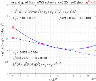
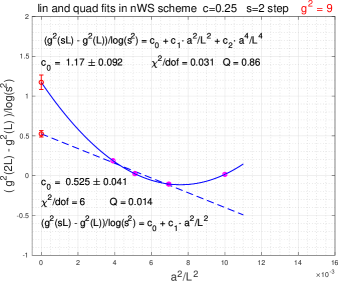
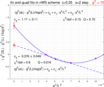
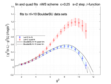
Figure 3: Our own fits are shown in four panels to the published $c=0.25$ data of [1].

We selected the preferred nWS scheme of the authors from data in Table III from [1]. Similarly to tests of our own lattice ensembles which we presented in Fig. 1 we are probing here the consistency of linear and quadratic fitting in $a^{2}/L^{2}$ for the DWF based step $\beta$-function in the continuum limit. Our linear fits in $a^{2}/L^{2}$ are in good agreement with the published fits of [1] for all three choices of $c$ with $c=0.25,0.275,0.30$ at each coupling. This is not the issue. Differing from [1], we also investigate quadratic fits in the $a^{2}/L^{2}$ variable over the entire $g^{2}=2-11$ range under consideration. Comparing linear and quadratic fits to the data of [1] at $c=0.25$ leads to rather peculiar results. The linear fitting hypothesis turns out to be unacceptable at strong couplings in the $g^{2}\approx 8-10.5$ range. The authors of [1] know that. Linear fitting works better at weaker couplings in the $g^{2}\approx 3-7$ range but rapidly deteriorates to unacceptable level toward $g^{2}\approx 8$ and remains unacceptable out to $g^{2}\approx 10$. At very strong coupling in the $g^{2}\approx 11-12$ range linear fits begin to work again in the nWS scheme but with rapidly increasing errors in the fits. Accepting the linear fits would lead to the IRFP, reached around $g^{2}\approx 11$. In sharp contrast, quadratic fitting in $a^{2}/L^{2}$ works well in the entire $g^{2}\approx 3-12$ range deteriorating below $g^{2}\approx 3$ which is irrelevant for the issue here. The nWS based quadratic fit to DWF data in Fig. 3 overshoots the results from our staggered fermion based fits peaking around $g^{2}\approx 9.5$ with $(g^{2}(sL)-g^{2}(L))/{\rm log}(s^{2})\approx 1.2$ of the step $\beta$-function and dropping back to $\beta\approx 0.95$ at $g^{2}=11$.

Based on our analysis, it is not credible to rely on the hypothesis of linear fits leading to the highly suspect IRFP at $c=0.25$. This would point then to the hypothesis of quadratic fits with much better statistical significance. However, the two hypotheses, both showing statistically acceptable fits to the continuum $\beta$-function outside the $g^{2}\approx 8-10$ range, should be compatible with each other for meaningful continuum fits. Unfortunately, they are not compatible, leading to paradoxical outcome in their predictions of the continuum limit, statistically far separated. Perhaps further scrutiny of the statistical analysis might resolve this contradiction. For example, quadratic DWF fits, extrapolating from small volumes to $L/a\rightarrow\infty$, are suspect with less controlled cutoff effects from smaller $L$ at shorter flow time. We speculate that larger volumes are needed for more consistent DWF analysis at $c=0.25$ for consistent linear and quadratic fits to the continuum limit.

2.4 Analysis of the finite volume based step $\beta$-function at c=0.275 and c=0.30

The two upper panels of the fits in Fig. 4 show our reasonably consistent fits with staggered fermions at $c=0.275$ in the $SSC$ and $SSS$ schemes at steps $s=2,3/2,4/3$, again without any indicator of an IRFP developing in the $g^{2}\approx 11-12$ range. Our own fits to the DWF data of  [1] changed somewhat. There are now statistically reasonable linear and quadratic fits to the data of [1] in the entire $g^{2}$ range but they are still incompatible with each other, separating around $g^{2}\approx 5$. The linear fits are closer to our fits in a broader $g^{2}$ range but separate around $g^{2}\approx 9-10$ with some significance. Our quadratic fits to DWF data from [1] significantly overshoot the fits to our staggered fermion based ensembles. We speculate again that the strange results the fitted DWF data exhibit is due to systematic difficulties when extrapolating to infinite lattice volumes from small DWF lattice.

The trends we observe at $c=0.275$ continue in $c=0.30$ based fits to the staggered fermion data and the DWF data as shown in Fig. 5. Our staggered fermion based analysis remains consistent and without any sign of an IRFP developing. There are again statistically reasonable linear and quadratic fits to the DWF data in the entire $g^{2}$ range but they are still incompatible with each other, separating around $g^{2}\approx 5$, similarly to the $c=0.275$ fits. The linear fits overlap with our staggered fermion fits below $g^{2}\approx 10$, with some separation setting in beyond.

In summary of all DWF fits analyzed for three choices of $c$, no signs were found for any indicator of conformal behavior in the ten-flavor theory. This is a significant disagreement from two independent lattice analyses of the same model and should warrant further discussion.

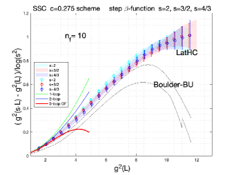
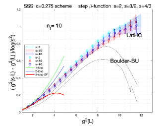
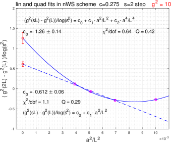
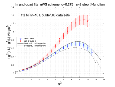
Figure 4: Results from LatHC staggered fermions at $c=0.275$ are shown in the two upper panels with fits from [1] also marked. Our own fits at $c=0.275$ to DWF data from [1] are shown in the two lower panels.

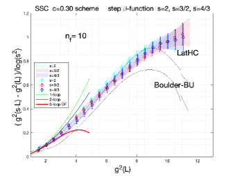
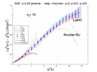
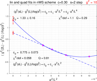
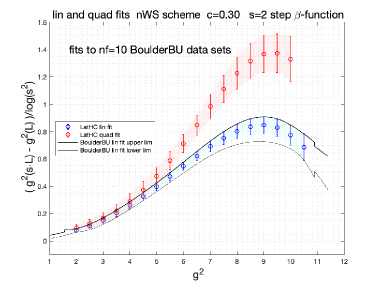
Figure 5: Fits at $c=0.30$ with respective upper and lower panels explained in the caption of Fig. 4.

2.5 The limits of lattice reach in the strong coupling regime

The nf = 10 $\beta$-functions of the staggered fermion formulation require the square root of the fermion determinant to obtain the correct flavor number in the continuum limit. We have previously provided a renormalization group based comprehensive theoretical argument to validate this procedure [23]. Implicit in the proof is the restoration of quartet degeneracy in the Dirac spectrum in the continuum limit. Once the quartet degeneracy is established in the Dirac spectrum toward the $a\rightarrow 0$ continuum limit, the rooted theory is expected to become equivalent to the correct continuum fermion theory. Toward the continuum limit eigenvalue pairs within quartets would start forming narrow doublets with two doublets split with more spacing within the quartet. Closer to the continuum limit doublets start merging into degenerate quartets. The emerging pattern is illustrated in Fig. 6 with the infrared part of the Dirac spectrum shown at the largest $48^{4}$ volume of the $L=32,36,40,48$ sequence we used in the earlier analysis with a set of bare gauge couplings in the $6/g_{0}^{2}=3-4$ range [5].

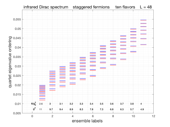
Figure 6: For illustration, the eigenvalue tower at the strongest bare coupling at $6/g_{0}^{2}=2.6$ of the extended work is shown in reaching toward the renormalized $g^{2}\approx 11$ range. The visible change in quartet ordering is discussed in the text.

It was shown that the infrared part of the Dirac determinant approached in the $a\rightarrow 0$ limit the fourth power of the determinant built from degenerate quartets, supporting the validation for the use of rooted determinants of staggered fermions [5]. The earlier analysis was extended for this report to ensembles with bare gauge couplings added in the $6/g_{0}^{2}=2.6-2.9$ strong coupling range to reach renormalized couplings in the $g^{2}\approx 11$ range. The added infrared eigenvalue tower at $6/g_{0}^{2}=2.6$ in Fig. 6 illustrates the challenge as we are pushing toward the limit of controlled lattice reach in the $g^{2}\approx 11$ range. The change in the spectrum at $6/g_{0}^{2}=2.6$ with significantly less quartet ordering of doublets is a first indicator of increased cutoff effects with delayed quartet degeneracy. Added larger volumes, like $L=64$, would help the convergence in reaching the continuum limit from an $L$-sequence of lattices.

More details will be provided about this analysis in the journal publication of this report.

3 The infinite-volume based continuum $\beta$-function in multi-flavor QCD at nf=10

3.1 Brief history and implementation of the method

We will discuss here new ten-flavor tests of the recently introduced lattice definition and algorithmic implementation of the $\beta$-function defined on the gradient flow of the gauge field over infinite Euclidean space-time in the continuum. The infinite-volume $\beta$-function is based directly on the gradient flow coupling $g^{2}(t)$ defined in infinite volume as a function of continuous flow time $t$. This will allow the direct definition $\beta(g^{2}(t))=t\cdot dg^{2}/dt$ from infinitesimal RG scale change using opposite sign convention from the conventional definition. The derivative will be approximated by five-point discretization of the flow time for any observable $E(t)$,

$$[-E(t+2\epsilon)+8E(t+\epsilon)-8E(t-\epsilon)+E(t-2\epsilon)]/(12\epsilon)=dE/dt+{\cal O}(\epsilon^{4}).$$ (3.1)

with discrete step $\epsilon$ used in the integration of the gradient flow equations. We tested several implementations and applications of the method [7, 6]. Originally we introduced this new algorithm to match finite-volume step $\beta$-functions in massless near-conformal gauge theories with the infinite-volume $\beta$-function in the chiral limit of fermion mass deformations from the phase with spontaneous chiral symmetry breaking. This implementation of the algorithm was tested first in a study of the near-conformal two-flavor sextet model reaching the chiral limit from small fermion mass deformations $m$ in the chiral symmetry breaking phase [7].

An alternative implementation of the infinite-volume $\beta$-function through $t\cdot dg^{2}/dt$, as applied here to the ten-flavor model, is based on simulations directly at $m=0$ and in the infinite-volume limit taken at fixed reference values of flow time $t/a^{2}$ in lattice units $a$. This lattice algorithm was first tested in the two-flavor QCD model [24] and in the multi-flavor nf=12 theory [6]. We will show in the ten-flavor lattice implementation how to make important contact at weak coupling with gradient flow based three-loop perturbation theory in infinite volume [11, 22], serving as a first pilot study toward the long-term goal of developing alternate approach to the determination of the strong coupling $\alpha_{s}$ at the Z-boson pole in QCD. It will be also shown that results from the lattice analysis of the infinite-volume based ten-flavor $\beta$-function are consistent with the absence of IRFP from our finite-volume ten-flavor step $\beta$-function in the range of renormalized couplings discussed in Section 2.

3.2 The ten-flavor lattice analysis

The algorithmic implementation of the lattice analysis has three steps.

Step 1: the four largest volumes $L^{4}=32^{4},36^{4},40^{4},48^{4}$ are selected for the analysis from the full set, discussed in Section 2, at 21 bare gauge couplings $6/g_{0}^{2}$ for each $L$ with periodic gauge and antiperiodic fermion boundary conditions. For the control of the continuum limit at zero lattice spacing, 12 preset values of the flow time $t$ were preselected for the agorithm at each $L$ and each $6/g_{0}^{2}$ starting at $t/a^{2}=2.5$ and extended to $t/a^{2}=8$ in increments of $0.5$ steps. We also preselect targeted $g^{2}$ values for the determination of the infinite volume based $\beta$-function in the limit of zero lattice spacing. We analyze here a choice of the preset range $g^{2}=1-10.5$ in increments of $0.5$. The preset $t/a^{2}$-sequence and $g^{2}$-sequence seem to be arbitrary but they are designed to sample the range of $g^{2}(t)$ in the continuum theory where the lattice spacing can be removed safely, based on fits to data from the selected lattice ensembles. Every preselected $g^{2}$ implicitly defines the flow time in the continuum at scale $\mu=1/\sqrt{8t}$. At each $L$ we calculate $g^{2}$ and its discretized $t\cdot dg^{2}/dt$ derivative on the gradient flow at 21 different $6/g_{0}^{2}$ couplings and at the 12 preselected $t/a^{2}$-values. At each $L$ we fit $t\cdot dg^{2}/dt$ as a function of $g^{2}$ to a fourth order polynomial at 21 points in $g^{2}$ and interpolate $t\cdot dg^{2}/dt$ from the polynomial fits to the preselected $g^{2}$ values at each preset $t/a^{2}$ for fixed $L$. Samples of this fitting procedure are shown in Fig. 7.

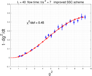
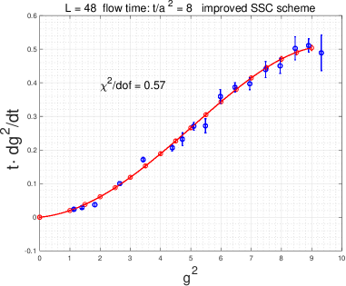
Figure 7: Fourth order polynomial fits of $t\cdot g^{2}/dt$ are shown in the $SSC$ scheme for $L=40$ and $L=48$ with good statistical quality. On the left panel the fit is shown to the fitted blue points $t\cdot g^{2}/dt$ for $L=40$ at locations of $g^{2}$ determined at bare gauge couplings at flow time $t/a^{2}=7$. The interpolated values of $t\cdot g^{2}/dt$ are marked with red symbols for targeted $g^{2}$ values. On the right panel similar fit and interpolation are shown for $L=48$ and $t/a^{2}=8$.

Step 2: The interpolated $L$-dependent $\beta=t\cdot dg^{2}/dt$ beta-functions are extrapolated to the infinite volume limit for each $t/a^{2}$ and each $g^{2}$ from Step 1, with samples of these fits shown in Fig 8.

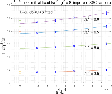
Figure 8: The interpolated $L$-dependent beta-functions of $\beta=t\cdot dg^{2}/dt$ are fitted to the $a^{2}/L^{2}\rightarrow 0$ infinite volume limit at fixed lattice spacing set by the four values of $t/a^{2}$ from the $2.5-8$ range at $g^{2}=8$. The fits with very good statistics are polynomials in the $a^{2}/L^{2}$ variable with a leading $a^{4}/L^{4}$ term and the higher order $a^{6}/L^{6}$ term with $L/a=32,36,40,48$ in the SSC scheme on the left and the SSS scheme on the right.

Step 3: After Step2 we have the infinite volume based beta-functions of $\beta=t\cdot dg^{2}/dt$ at 12 values of $t/a^{2}$ for each targeted value of the gradient flow based renormalized coupling $g^{2}$ held fixed in the algorithm. In Step 3, we fit the cutoff dependence of $\beta=t\cdot dg^{2}/dt$ to determine its $a\rightarrow 0$ continuum limit at fixed $g^{2}$. This is obtained by quadratic fits in the $a^{2}/t$ variable with fit samples shown in Fig. 9. If the correlated fits of the three steps are statistically consistent and acceptable, we reached the goal in the covered and sampled $g^{2}=1.5-10.5$ range which can be extended by added analysis.

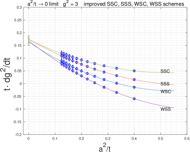
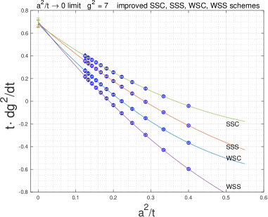
Figure 9: Continuum fits of $\beta=t\cdot dg^{2}/dt$ are shown in all four schemes at two renormalized couplings with choices of $g^{2}=3$ and $g^{2}=7$. The fits are quadratic in the $a^{2}/t$ variable.

3.3 Ten-flavor tests toward the goal of the strong coupling $\alpha_{s}$ at the Z-pole in QCD

After the three-step analysis of the ten-flavor model we reached the set goal of $\beta(g^{2}(t))=t\cdot dg^{2}/dt$ in the $g^{2}(t)=1.5-10.5$ range, as shown in Fig. 10.

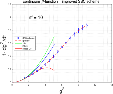
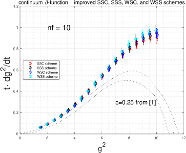
Figure 10: The dashed line in the left panel shows spline based fitting in the $g^{2}=3-9$ range of the SSC scheme. The fit would be identical in the SSS scheme, or in the WSC and WSS schemes, added in the right panel. Below $g^{2}=3$ three-loop perturbation theory can be used for the $\beta$-function from [11, 22].

The value of $g^{2}(t)$ implicitly defines the scale $\mu=1/\sqrt{8t}$ which ultimately would be connected to a nonperturbative parameter, like the decay constant $f=F_{\pi}$ of the Goldstone pion, if the theory turns out to be near-conformal with spontaneous chiral symmetry breaking. Similar to [25] in three-flavor QCD with massless fermions, we can connect now the $\Lambda_{GF}$ scale of the gradient flow scheme to other scales, like the scale $\mu=1/\sqrt{8t}$ set by the choice $g^{2}(t)$ in the ten-flavor theory with massless fermions. As an example, we will express the scale $L_{0}=\sqrt{8t}$ set at ${\bar{g}}^{2}=5$ in $\Lambda_{GF}$ units of the ten-flavor theory,

$$L_{0}\cdot\Lambda_{GF}=(b_{0}{\bar{g}}^{2})^{-b_{1}/2b_{0}^{2}}\cdot{\rm exp}(-1/2b_{0}{\bar{g}}^{2})\cdot{\rm exp}\Bigl{(}-\int_{0}^{\bar{g}}dx\bigl{[}1/\beta(x)+1/b_{0}x^{3}-b_{1}/b_{0}^{2}x\bigr{]}\Bigr{)}.$$ (3.2)

The integral in Eq.(3.2) was broken up into two parts. In the $x=0-3$ range the three-loop value of the $\beta$-function was used and the $x=3-5$ range was evaluated with numerical

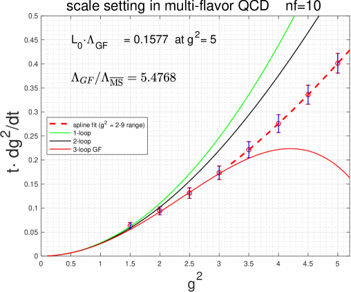
Figure 11: The dashed line in the figure shows spline based fitting in the $g^{2}=3-9$ range of the SSC scheme. Below $g^{2}=3$ three-loop perturbation theory can be used for the $\beta$-function from [11, 22].

integration, based on the spline fit made to the data. The result of $L_{0}\cdot\Lambda_{GF}=0.1577$ can be converted to $\Lambda_{\overline{\rm MS}}$ units of the ten-flavor theory, $L_{0}\cdot\Lambda_{\overline{\rm MS}}=0.02879$, using the conversion factor $\Lambda_{GF}/\Lambda_{\overline{\rm MS}}=5.4768$ from a well-know one-loop calculation [11, 22]. The precision of the calculation is on the few percent level with combined systematic and statistical uncertainties, not far from the goal of performing similar analysis in three-flavor QCD with massless fermions. Conclusions: We have presented strong evidence from our finite volume based step $\beta$-function analysis that massless multi-flavor QCD with ten flavors shows no IRFP, or any hint for it within controlled lattice reach with added support from the infinite volume based $\beta$-function. Scale setting of the gradient flow time at selected $g^{2}(t)$ values, defined over unlimited Euclidean space-time, was successfully demonstrated in $\Lambda_{\overline{\rm MS}}$ units of the theory using the infinite volume based ten-flavor $\beta$-function. This holds promise for alternate determination of the strong coupling $\alpha_{s}$ in QCD.

Appendix

Appendix A Polynomial interpolations in the c=0.25 and c=0.30 step $\beta$-function schemes

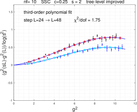
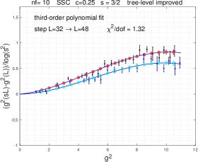
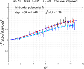
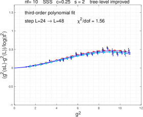
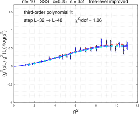
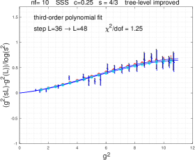
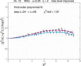
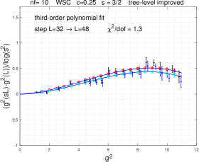
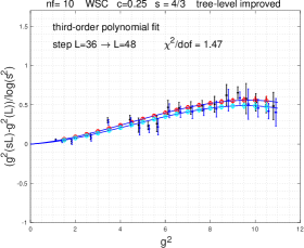
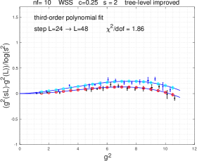
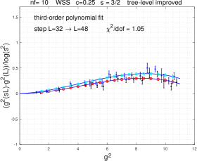
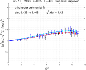
Figure A.1: Polynomial fits and interpolations are shown at $c=0.25$ for lattice step functions $(g^{2}(sL)-g^{2}(L))/{\rm log}(s^{2})$ with and without tree-level improvement for the $L=24\rightarrow L=48$ pair with step $s=2$, $L=32\rightarrow L=48$ at $s=3/2$, and $L=36\rightarrow L=48$ at $s=4/3$. 4th order polynomials are used in $g^{2}$ and constrained to vanish at $g^{2}=0$. Red circles mark the lattice step $\beta$-functions at targeted $g^{2}$ locations in the unimproved schemes and cyan circles are the targets with tree-level improvement. Fits to the measured data points at bare couplings $g_{0}^{2}$ are shown in black for unimproved data and in blue for tree-improved data.

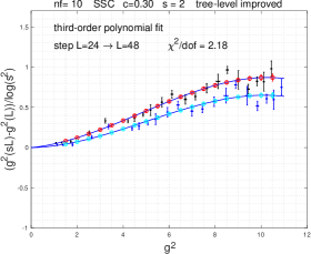
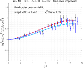
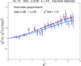
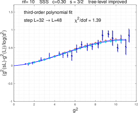
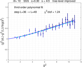
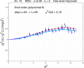
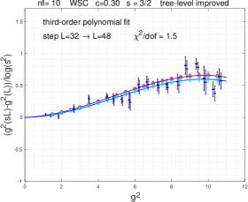
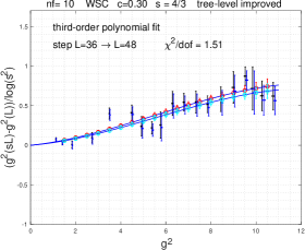
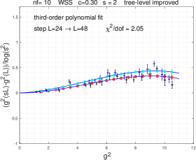
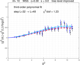
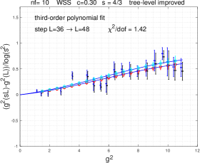
Figure A.2: The fitting procedure is similar to what is described in Fig. A.1 and in the main text.

References

- [1] A. Hasenfratz, C. Rebbi, O. Witzel, Gradient flow step-scaling function for SU(3) with ten fundamental flavors, Phys. Rev. D 101 (11) (2020) 114508. arXiv:2004.00754, doi:10.1103/PhysRevD.101.114508.
- [2] T. Appelquist, et al., Near-conformal dynamics in a chirally broken system, Phys. Rev. D 103 (1) (2021) 014504. arXiv:2007.01810, doi:10.1103/PhysRevD.103.014504.
- [3] T.-W. Chiu, Discrete -function of the gauge theory with 10 massless domain-wall fermions, PoS LATTICE2016 (2017) 228. doi:10.22323/1.256.0228.
- [4] T.-W. Chiu, Improved study of the -function of gauge theory with massless domain-wall fermions, Phys. Rev. D 99 (1) (2019) 014507. arXiv:1811.01729, doi:10.1103/PhysRevD.99.014507.
- [5] Z. Fodor, K. Holland, J. Kuti, D. Nogradi, C. H. Wong, Fate of a recent conformal fixed point and -function in the SU(3) BSM gauge theory with ten massless flavors, PoS LATTICE2018 (2018) 199. arXiv:1812.03972, doi:10.22323/1.334.0199.
- [6] Z. Fodor, K. Holland, J. Kuti, D. Nogradi, C. H. Wong, Case studies of near-conformal -functions, PoS LATTICE2019 (2019) 121. arXiv:1912.07653, doi:10.22323/1.363.0121.
- [7] Z. Fodor, K. Holland, J. Kuti, D. Nogradi, C. H. Wong, A new method for the beta function in the chiral symmetry broken phase, EPJ Web Conf. 175 (2018) 08027. arXiv:1711.04833, doi:10.1051/epjconf/201817508027.
- [8] R. Narayanan, H. Neuberger, Infinite N phase transitions in continuum Wilson loop operators, JHEP 03 (2006) 064. arXiv:hep-th/0601210, doi:10.1088/1126-6708/2006/03/064.
- [9] M. Lüscher, Properties and uses of the Wilson flow in lattice QCD, JHEP 08 (2010) 071. doi:10.1007/JHEP08(2010)071,10.1007/JHEP03(2014)092.
- [10] M. Luscher, Topology, the Wilson flow and the HMC algorithm, PoS LATTICE2010 (2010) 015. arXiv:1009.5877.
- [11] R. V. Harlander, T. Neumann, The perturbative QCD gradient flow to three loops, JHEP 06 (2016) 161. arXiv:1606.03756, doi:10.1007/JHEP06(2016)161.
- [12] Work in collaboration with Szabolcs Borsányi.
- [13] M. Luscher, Trivializing maps, the Wilson flow and the HMC algorithm, Commun. Math. Phys. 293 (2010) 899–919. arXiv:0907.5491, doi:10.1007/s00220-009-0953-7.
- [14] M. Luscher, P. Weisz, Perturbative analysis of the gradient flow in non-abelian gauge theories, JHEP 02 (2011) 051. doi:10.1007/JHEP02(2011)051.
- [15] R. Lohmayer, H. Neuberger, Continuous smearing of Wilson Loops, PoS LATTICE2011 (2011) 249. arXiv:1110.3522.
- [16] M. Lüscher, Future applications of the Yang-Mills gradient flow in lattice QCD, PoS LATTICE2013 (2014) 016. arXiv:1308.5598, doi:10.22323/1.187.0016.
- [17] S. Borsanyi, et al., High-precision scale setting in lattice QCD, JHEP 09 (2012) 010. arXiv:1203.4469, doi:10.1007/JHEP09(2012)010.
- [18] Z. Fodor, K. Holland, J. Kuti, D. Nogradi, C. H. Wong, The Yang-Mills gradient flow in finite volume, JHEP 11 (2012) 007. arXiv:1208.1051, doi:10.1007/JHEP11(2012)007.
- [19] M. Luscher, R. Narayanan, P. Weisz, U. Wolff, The Schrodinger functional: A Renormalizable probe for nonAbelian gauge theories, Nucl. Phys. B384 (1992) 168–228. arXiv:hep-lat/9207009, doi:10.1016/0550-3213(92)90466-O.
- [20] Z. Fodor, K. Holland, J. Kuti, S. Mondal, D. Nogradi, C. H. Wong, Fate of the conformal fixed point with twelve massless fermions and SU(3) gauge group, Phys. Rev. D94 (9) (2016) 091501. arXiv:1607.06121, doi:10.1103/PhysRevD.94.091501.
- [21] Z. Fodor, K. Holland, J. Kuti, S. Mondal, D. Nogradi, C. H. Wong, The lattice gradient flow at tree-level and its improvement, JHEP 09 (2014) 018. arXiv:1406.0827, doi:10.1007/JHEP09(2014)018.
- [22] J. Artz, R. V. Harlander, F. Lange, T. Neumann, M. Prausa, Results and techniques for higher order calculations within the gradient-flow formalism, JHEP 06 (2019) 121, [Erratum: JHEP 10, 032 (2019)]. arXiv:1905.00882, doi:10.1007/JHEP06(2019)121.
- [23] Z. Fodor, K. Holland, J. Kuti, S. Mondal, D. Nogradi, C. H. Wong, The running coupling of the minimal sextet composite Higgs model, JHEP 09 (2015) 039. arXiv:1506.06599, doi:10.1007/JHEP09(2015)039.
- [24] A. Hasenfratz, O. Witzel, Continuous renormalization group function from lattice simulations, Phys. Rev. D 101 (3) (2020) 034514. arXiv:1910.06408, doi:10.1103/PhysRevD.101.034514.
- [25] M. Dalla Brida, P. Fritzsch, T. Korzec, A. Ramos, S. Sint, R. Sommer, A non-perturbative exploration of the high energy regime in QCD, Eur. Phys. J. C 78 (5) (2018) 372. arXiv:1803.10230, doi:10.1140/epjc/s10052-018-5838-5.