=log_2(1+$\gamma_{i}^{\text{\tiny NOMA}}$).UNKNOWNUNKNOWN{} (4)

Further, based on principle [NomaPrinciple], the following conditions hold.

$$\alpha_{\text{\scriptsize G}}>\alpha_{\text{\scriptsize G}-1}>...>\alpha_{2}>\alpha_{1}$$ (5)
$$\sum_{i=1}^{G}\alpha_{i}=1.\hskip 11.38092pt$$ (6)

From (5), we conclude the following result

$\displaystyle\sum_{j=i+1}^{G}\alpha_{j}$ $\displaystyle>(G-i)\alpha_{i}.$ (7)

Next, we present the bounds on power allocation factors and channel coefficients for users in a cluster in the presence of imperfections in .

III Computation of Bounds

In this section, we derive a lower bound on the power allocation factor and an upper bound on the imperfections in for a cluster under consideration in terms of channel coefficients. Further, we formulate criterion for a multi-user cluster to achieve higher user rates as compared to .

III-A Lower Bound on $\alpha_{i}$

We consider the rate of each individual user should be greater than the rate (RiNOMA>RiOMARiNOMARiOMA\lx@glossaries@gls@link{main}{RNOMA}{\leavevmode R_{i}^{\text{\tiny NOMA}}}>\lx@glossaries@gls@link{main}{ROMA}{\leavevmode R_{i}^{\text{\tiny OMA}}}). Thus, from (LABEL:eqn:ROMA) and (4), we have

log2(1+γiNOMA)subscript21γiNOMA\displaystyle\log_{2}(1+\lx@glossaries@gls@link{main}{GammaNOMA}{\leavevmode\gamma_{i}^{\text{\tiny NOMA}}}) >1Glog2(1+γiOMA), yieldingabsent1Gsubscript21γiOMA yielding\displaystyle>\dfrac{1}{\lx@glossaries@gls@link{main}{G}{\leavevmode G}}\log_{2}(1+\lx@glossaries@gls@link{main}{GammaOMA}{\leavevmode\gamma_{i}^{\text{\tiny OMA}}}),\textmd{ yielding}
γiNOMA >[1+γiOMA]1G1.absentsuperscriptdelimited-[]1γiOMA1G1\displaystyle>\left[1+\lx@glossaries@gls@link{main}{GammaOMA}{\leavevmode\gamma_{i}^{\text{\tiny OMA}}}\right]^{\frac{1}{\lx@glossaries@gls@link{main}{G}{\leavevmode G}}}-1. (8)

Using $\gamma_{i}^{\text{\tiny NOMA}}$ from (LABEL:eqn:GammaNOMA) in (8), we have

αiγiOMA1+j=1,jii1αjγiOMA+βj=i+1GαjγiOMAαiγiOMA1superscriptsubscriptformulae-sequence𝑗1𝑗𝑖𝑖1subscript𝛼𝑗γiOMAβsuperscriptsubscript𝑗𝑖1Gsubscript𝛼𝑗γiOMA\displaystyle\dfrac{\lx@glossaries@gls@link{main}{alphai}{\leavevmode\alpha_{i}}\lx@glossaries@gls@link{main}{GammaOMA}{\leavevmode\gamma_{i}^{\text{\tiny OMA}}}}{1+\sum_{j=1,j\neq i}^{i-1}\alpha_{j}\lx@glossaries@gls@link{main}{GammaOMA}{\leavevmode\gamma_{i}^{\text{\tiny OMA}}}+\lx@glossaries@gls@link{main}{beta}{\leavevmode\beta}\sum_{j=i+1}^{\lx@glossaries@gls@link{main}{G}{\leavevmode G}}\alpha_{j}\lx@glossaries@gls@link{main}{GammaOMA}{\leavevmode\gamma_{i}^{\text{\tiny OMA}}}} >[1+γiOMA]1G1.absentsuperscriptdelimited-[]1γiOMA1G1\displaystyle>\left[1+\lx@glossaries@gls@link{main}{GammaOMA}{\leavevmode\gamma_{i}^{\text{\tiny OMA}}}\right]^{\frac{1}{\lx@glossaries@gls@link{main}{G}{\leavevmode G}}}-1.

Substituting $\sum_{j=1,j\neq i}^{i-1}\alpha_{j}=1-\alpha_{i}-\sum_{j=i+1}^{G}\alpha_{j}$ from (6), we get

αi1+[1+(β1)j=i+1Gαjαi]γiOMA>[1+γiOMA]1G1γiOMA.αi1delimited-[]1𝛽1superscriptsubscript𝑗𝑖1Gsubscript𝛼𝑗subscript𝛼𝑖γiOMAsuperscriptdelimited-[]1γiOMA1G1γiOMA\displaystyle\dfrac{\lx@glossaries@gls@link{main}{alphai}{\leavevmode\alpha_{i}}}{1+\Big{[}1+(\beta-1)\sum_{j=i+1}^{\lx@glossaries@gls@link{main}{G}{\leavevmode G}}\alpha_{j}-\alpha_{i}\Big{]}\lx@glossaries@gls@link{main}{GammaOMA}{\leavevmode\gamma_{i}^{\text{\tiny OMA}}}}>\dfrac{\left[1+\lx@glossaries@gls@link{main}{GammaOMA}{\leavevmode\gamma_{i}^{\text{\tiny OMA}}}\right]^{\frac{1}{\lx@glossaries@gls@link{main}{G}{\leavevmode G}}}-1}{\lx@glossaries@gls@link{main}{GammaOMA}{\leavevmode\gamma_{i}^{\text{\tiny OMA}}}}.

Solving it further, we obtain lower bound on $\alpha_{i}$ as follows:

αi>(1+(1+(β1)j=i+1Gαj)γiOMA)((1+γiOMA)1G1γiOMA(1+γiOMA)1G).αi11𝛽1superscriptsubscript𝑗𝑖1Gsubscript𝛼𝑗γiOMAsuperscript1γiOMA1𝐺1γiOMAsuperscript1γiOMA1G\displaystyle\lx@glossaries@gls@link{main}{alphai}{\leavevmode\alpha_{i}}>\Big{(}{1+\big{(}1+(\beta-1)\sum_{j=i+1}^{\lx@glossaries@gls@link{main}{G}{\leavevmode G}}\alpha_{j}\big{)}\lx@glossaries@gls@link{main}{GammaOMA}{\leavevmode\gamma_{i}^{\text{\tiny OMA}}}}\Big{)}\Bigg{(}\dfrac{(1+\lx@glossaries@gls@link{main}{GammaOMA}{\leavevmode\gamma_{i}^{\text{\tiny OMA}}})^{\frac{1}{G}}-1}{\lx@glossaries@gls@link{main}{GammaOMA}{\leavevmode\gamma_{i}^{\text{\tiny OMA}}}(1+\lx@glossaries@gls@link{main}{GammaOMA}{\leavevmode\gamma_{i}^{\text{\tiny OMA}}})^{\frac{1}{\lx@glossaries@gls@link{main}{G}{\leavevmode G}}}}\Bigg{)}. (9)

For the ease of understanding, we define

?(χG)(γiOMA)=?(χG)γiOMAabsent\displaystyle\lx@glossaries@gls@link{main}{Ffun}{\leavevmode?(\chi_{\text{\tiny G}})}(\lx@glossaries@gls@link{main}{GammaOMA}{\leavevmode\gamma_{i}^{\text{\tiny OMA}}})= (1+γiOMA)1G1γiOMA(1+γiOMA)1G.superscript1γiOMA1𝐺1γiOMAsuperscript1γiOMA1G\displaystyle\dfrac{(1+\lx@glossaries@gls@link{main}{GammaOMA}{\leavevmode\gamma_{i}^{\text{\tiny OMA}}})^{\frac{1}{G}}-1}{\lx@glossaries@gls@link{main}{GammaOMA}{\leavevmode\gamma_{i}^{\text{\tiny OMA}}}(1+\lx@glossaries@gls@link{main}{GammaOMA}{\leavevmode\gamma_{i}^{\text{\tiny OMA}}})^{\frac{1}{\lx@glossaries@gls@link{main}{G}{\leavevmode G}}}}. (10)

Using (10), we reformulate (9) as αi>?(δi)αi?(δi)\lx@glossaries@gls@link{main}{alphai}{\leavevmode\alpha_{i}}>\lx@glossaries@gls@link{main}{Delta}{\leavevmode?(\delta_{i})}, where

δi=δiabsent\displaystyle\lx@glossaries@gls@link{main}{Delta}{\leavevmode\delta_{i}}= (1+(1+(β1)j=i+1Gαj)γiOMA)χG(γiOMA).11𝛽1superscriptsubscript𝑗𝑖1Gsubscript𝛼𝑗γiOMAχGγiOMA\displaystyle\Big{(}{1+\big{(}1+(\beta-1)\sum_{j=i+1}^{\lx@glossaries@gls@link{main}{G}{\leavevmode G}}\alpha_{j}\big{)}\lx@glossaries@gls@link{main}{GammaOMA}{\leavevmode\gamma_{i}^{\text{\tiny OMA}}}}\Big{)}\lx@glossaries@gls@link{main}{Ffun}{\leavevmode\chi_{\text{\tiny G}}}(\lx@glossaries@gls@link{main}{GammaOMA}{\leavevmode\gamma_{i}^{\text{\tiny OMA}}}). (11)

Substituting (7) in (11), we get

δi<(1+(1+(β1)(Gi)αi)γiOMA)χG(γiOMA).δi11𝛽1𝐺𝑖subscript𝛼𝑖γiOMAχGγiOMA\displaystyle\lx@glossaries@gls@link{main}{Delta}{\leavevmode\delta_{i}}<\Big{(}{1+\Big{(}1+(\beta-1)(G-i)\alpha_{i}\Big{)}\lx@glossaries@gls@link{main}{GammaOMA}{\leavevmode\gamma_{i}^{\text{\tiny OMA}}}}\Big{)}\lx@glossaries@gls@link{main}{Ffun}{\leavevmode\chi_{\text{\tiny G}}}(\lx@glossaries@gls@link{main}{GammaOMA}{\leavevmode\gamma_{i}^{\text{\tiny OMA}}}). (12)

Thus, if αi>(1+(1+(β1)(Gi)αi)γiOMA)χG(γiOMA)αi11𝛽1𝐺𝑖subscript𝛼𝑖γiOMAχGγiOMA\lx@glossaries@gls@link{main}{alphai}{\leavevmode\alpha_{i}}>\Big{(}{1+\Big{(}1+(\beta-1)(G-i)\alpha_{i}\Big{)}\lx@glossaries@gls@link{main}{GammaOMA}{\leavevmode\gamma_{i}^{\text{\tiny OMA}}}}\Big{)}\lx@glossaries@gls@link{main}{Ffun}{\leavevmode\chi_{\text{\tiny G}}}(\lx@glossaries@gls@link{main}{GammaOMA}{\leavevmode\gamma_{i}^{\text{\tiny OMA}}}), then, αi>δiαiδi\lx@glossaries@gls@link{main}{alphai}{\leavevmode\alpha_{i}}>\lx@glossaries@gls@link{main}{Delta}{\leavevmode\delta_{i}}. Solving αi further, we obtain

αi >(1+γiOMA)χG(γiOMA)1(β1)(Gi)γiOMAχG(γiOMA).absent1γiOMAχGγiOMA1β1𝐺𝑖γiOMAχGγiOMA\displaystyle>\dfrac{(1+\lx@glossaries@gls@link{main}{GammaOMA}{\leavevmode\gamma_{i}^{\text{\tiny OMA}}})\lx@glossaries@gls@link{main}{Ffun}{\leavevmode\chi_{\text{\tiny G}}}(\lx@glossaries@gls@link{main}{GammaOMA}{\leavevmode\gamma_{i}^{\text{\tiny OMA}}})}{1-(\lx@glossaries@gls@link{main}{beta}{\leavevmode\beta}-1)(G-i)\lx@glossaries@gls@link{main}{GammaOMA}{\leavevmode\gamma_{i}^{\text{\tiny OMA}}}\lx@glossaries@gls@link{main}{Ffun}{\leavevmode\chi_{\text{\tiny G}}}(\lx@glossaries@gls@link{main}{GammaOMA}{\leavevmode\gamma_{i}^{\text{\tiny OMA}}})}. (13)

Note that if (13) is satisfied, then $R_{i}^{\text{\tiny NOMA}}$ is always greater than $R_{i}^{\text{\tiny OMA}}$. Further, (9) is a sufficient condition to achieve higher rates, whereas (13) is a much stricter bound as compared to (9). Since (13) is dependent only on $\gamma_{i}^{\text{\tiny OMA}}$ and $G$, we use (13) to define constraints for multi-user clustering.

III-B Upper Bound on the Imperfect SIC Parameter (β)

From (5), $\alpha_{i}>\alpha_{i-1}$. Using the bounds in (13), we get

(1+γiOMA)χG(γiOMA)1(β1)(Gi)γiOMAχG(γiOMA)1superscriptsubscript𝛾𝑖OMAχGsuperscriptsubscript𝛾𝑖OMA1β1𝐺𝑖superscriptsubscript𝛾𝑖OMAχGsuperscriptsubscript𝛾𝑖OMA\displaystyle\dfrac{(1+\gamma_{i}^{\text{\tiny OMA}})\lx@glossaries@gls@link{main}{Ffun}{\leavevmode\chi_{\text{\tiny G}}}(\gamma_{i}^{\text{\tiny OMA}})}{1-(\lx@glossaries@gls@link{main}{beta}{\leavevmode\beta}-1)(G-i)\gamma_{i}^{\text{\tiny OMA}}\lx@glossaries@gls@link{main}{Ffun}{\leavevmode\chi_{\text{\tiny G}}}(\gamma_{i}^{\text{\tiny OMA}})}
>(1+γi1OMA)χG(γi1OMA)1(β1)(Gi+1)γi1OMAχG(γi1OMA).absent1superscriptsubscript𝛾𝑖1OMAχGsuperscriptsubscript𝛾𝑖1OMA1β1𝐺𝑖1superscriptsubscript𝛾𝑖1OMAχGsuperscriptsubscript𝛾𝑖1OMA\displaystyle>\dfrac{(1+\gamma_{i-1}^{\text{\tiny OMA}})\lx@glossaries@gls@link{main}{Ffun}{\leavevmode\chi_{\text{\tiny G}}}(\gamma_{i-1}^{\text{\tiny OMA}})}{1-(\lx@glossaries@gls@link{main}{beta}{\leavevmode\beta}-1)(G-i+1)\gamma_{i-1}^{\text{\tiny OMA}}\lx@glossaries@gls@link{main}{Ffun}{\leavevmode\chi_{\text{\tiny G}}}(\gamma_{i-1}^{\text{\tiny OMA}})}. (14)

For ease of exposition, we define the following terms

$\displaystyle D_{i}$ =(1+γi1OMA)χG(γi1OMA)(1+γiOMA)χG(γiOMA),Ei=(Gi)γiOMAχG(γiOMA),formulae-sequenceabsent1superscriptsubscript𝛾𝑖1OMAχGsuperscriptsubscript𝛾𝑖1OMA1superscriptsubscript𝛾𝑖OMAχGsuperscriptsubscript𝛾𝑖OMAsubscript𝐸𝑖𝐺𝑖superscriptsubscript𝛾𝑖OMAχGsuperscriptsubscript𝛾𝑖OMA\displaystyle=\dfrac{(1+\gamma_{i-1}^{\text{\tiny OMA}})\lx@glossaries@gls@link{main}{Ffun}{\leavevmode\chi_{\text{\tiny G}}}(\gamma_{i-1}^{\text{\tiny OMA}})}{(1+\gamma_{i}^{\text{\tiny OMA}})\lx@glossaries@gls@link{main}{Ffun}{\leavevmode\chi_{\text{\tiny G}}}(\gamma_{i}^{\text{\tiny OMA}})},E_{i}=(G-i)\gamma_{i}^{\text{\tiny OMA}}\lx@glossaries@gls@link{main}{Ffun}{\leavevmode\chi_{\text{\tiny G}}}(\gamma_{i}^{\text{\tiny OMA}}),
$\displaystyle E_{i-1}$ =(Gi+1)γi1OMAχG(γi1OMA).absent𝐺𝑖1superscriptsubscript𝛾𝑖1OMAχGsuperscriptsubscript𝛾𝑖1OMA\displaystyle=(G-i+1)\gamma_{i-1}^{\text{\tiny OMA}}\lx@glossaries@gls@link{main}{Ffun}{\leavevmode\chi_{\text{\tiny G}}}(\gamma_{i-1}^{\text{\tiny OMA}}).

Substituting $D_{i}$, $E_{i}$ and $E_{i-1}$ in (14), we get

1(β1)Ei11β1subscript𝐸𝑖1\displaystyle 1-(\lx@glossaries@gls@link{main}{beta}{\leavevmode\beta}-1)E_{i-1} >Di[1(β1)Ei],absentsubscript𝐷𝑖delimited-[]1β1subscript𝐸𝑖\displaystyle>D_{i}\big{[}1-(\lx@glossaries@gls@link{main}{beta}{\leavevmode\beta}-1)E_{i}\big{]}, (15)
β $\displaystyle<\dfrac{1-D_{i}}{E_{i-1}-D_{i}E_{i}}+1\triangleq\zeta_{i-1,i}.$ (16)

Thus, for the rates to be higher than the rates, the typical value of imperfections in must satisfy the constraint in (16) for the multi-user clustering in under consideration.

III-C between Successive Users

In case of G users clustered in system, we define the between two users for achieving higher rates as follows. We apply positivity constraint β>0β0\lx@glossaries@gls@link{main}{beta}{\leavevmode\beta}>0 in (16), thus,

$\displaystyle 1-D_{i}>D_{i}E_{i}-E_{i-1}\rightarrow E_{i-1}>D_{i}E_{i}+D_{i}-1.$ (17)

Substituting $E_{i-1}$ from (III-B) in (17), we get

(Gi+1)γi1OMAχG(γi1OMA)𝐺𝑖1superscriptsubscript𝛾𝑖1OMAχGsuperscriptsubscript𝛾𝑖1OMA\displaystyle(G-i+1)\gamma_{i-1}^{\text{\tiny OMA}}\lx@glossaries@gls@link{main}{Ffun}{\leavevmode\chi_{\text{\tiny G}}}(\gamma_{i-1}^{\text{\tiny OMA}}) $\displaystyle>D_{i}E_{i}+D_{i}-1,$
$\displaystyle\gamma_{i-1}^{\text{\tiny OMA}}$ >DiEi+Di1(Gi+1)χG(γi1OMA),absentsubscript𝐷𝑖subscript𝐸𝑖subscript𝐷𝑖1𝐺𝑖1χGsuperscriptsubscript𝛾𝑖1OMA\displaystyle>\dfrac{D_{i}E_{i}+D_{i}-1}{(G-i+1)\lx@glossaries@gls@link{main}{Ffun}{\leavevmode\chi_{\text{\tiny G}}}(\gamma_{i-1}^{\text{\tiny OMA}})},
$\displaystyle\gamma_{i-1}^{\text{\tiny OMA}}-\gamma_{i}^{\text{\tiny OMA}}$ >DiEi+Di1(Gi+1)χG(γi1OMA)γiOMA.absentsubscript𝐷𝑖subscript𝐸𝑖subscript𝐷𝑖1𝐺𝑖1χGsuperscriptsubscript𝛾𝑖1OMAsuperscriptsubscript𝛾𝑖OMA\displaystyle>\dfrac{D_{i}E_{i}+D_{i}-1}{(G-i+1)\lx@glossaries@gls@link{main}{Ffun}{\leavevmode\chi_{\text{\tiny G}}}(\gamma_{i-1}^{\text{\tiny OMA}})}-\gamma_{i}^{\text{\tiny OMA}}.

Thus, we define the between users $i-1$ and $i$ as follows

?(ΔMSDi-1,i)=DiEi+Di1(Gi+1)χG(γi1OMA)γiOMA.?(ΔMSDi-1,i)subscript𝐷𝑖subscript𝐸𝑖subscript𝐷𝑖1𝐺𝑖1χGsuperscriptsubscript𝛾𝑖1OMAsuperscriptsubscript𝛾𝑖OMA\displaystyle\lx@glossaries@gls@link{main}{DeltaMSD}{\leavevmode?(\Delta^{\tiny MSD}_{\tiny i-1,i})}=\dfrac{D_{i}E_{i}+D_{i}-1}{(G-i+1)\lx@glossaries@gls@link{main}{Ffun}{\leavevmode\chi_{\text{\tiny G}}}(\gamma_{i-1}^{\text{\tiny OMA}})}-\gamma_{i}^{\text{\tiny OMA}}. (18)

Note that for a cluster of $G$ users, we have $G-1$ combinations of $\Delta^{\tiny MSD}_{\tiny i-1,i}$ and $\zeta_{i-1,i}$ values. In case (16) and (18) are satisfied for all these combinations, then all the $G$ users can be clustered together to achieve rates higher than their counterparts. Further, we next use the formulated in (18) and the lower bound on power allocation formulated in (9) to propose MUC, AMUC and power allocation algorithms for systems, respectively.

Refer to caption
Figure 2: Various user clustering scenarios for multi-user .

IV Proposed Algorithms

In this section, we explain the procedure for the clustering of users. We propose MUC and AMUC algorithms to achieve higher user rates and compare their performance with a conventional near-far (NF) [NearFar2] user pairing algorithm. Given a set of users in a cluster, we then present power allocation for each user.

Refer to caption
Figure 3: Splitting of a 4 user cluster into two 2 user clusters.
Input : $U$, $\gamma_{\text{i}}^{\text{\tiny OMA}}$, $N$, $G$, $\beta$.
Variables : $r$ and $i$ are variables representing cluster index and user index, respectively. Flag is a variable used to keep track of criterion.
1 Function Clustering($U$, $G$, $N$):
2       $U^{\prime}=\texttt{sort}(U,\texttt{`descend'})$;
3       $U^{\prime\prime}\leftarrow$ Reshape $U^{\prime}$ into $G$ columns;
4       $U_{\text{\tiny\it Clustered}}\leftarrow$ Flip users of $U^{\prime\prime}$ in columns $\frac{G}{2}$ to $G$;
5       for  $r=1\rightarrow\frac{N}{G}$ do
6             $U_{r}\leftarrow$ Pick $G$ users from $r^{th}$ row of $U_{\text{\tiny\it Clustered}}$;
7             for $i=2\rightarrow G$ do
8                  if  β<ζi1,iβsubscript𝜁𝑖1𝑖\lx@glossaries@gls@link{main}{beta}{\leavevmode\beta}<\zeta_{i-1,i} and γi1OMAγiOMA>ΔMSDi-1,isuperscriptsubscript𝛾𝑖1OMAsuperscriptsubscript𝛾𝑖OMAΔMSDi-1,i\gamma_{i-1}^{\text{\tiny OMA}}-\gamma_{i}^{\text{\tiny OMA}}>\lx@glossaries@gls@link{main}{DeltaMSD}{\leavevmode\Delta^{\tiny MSD}_{\tiny i-1,i}}  then
9                        Flag=0;
10                         for $i=G\rightarrow 1$ do
11                              αi=(1+(1j=i+1Gαj)γiOMA)χG(γiOMA\lx@glossaries@gls@link{main}{alphai}{\leavevmode\alpha_{i}}=\Big{(}{1+\big{(}1-\sum_{j=i+1}^{\lx@glossaries@gls@link{main}{G}{\leavevmode G}}\alpha_{j}\big{)}\lx@glossaries@gls@link{main}{GammaOMA}{\leavevmode\gamma_{i}^{\text{\tiny OMA}}}}\Big{)}\lx@glossaries@gls@link{main}{Ffun}{\leavevmode\chi_{\text{\tiny G}}}(\lx@glossaries@gls@link{main}{GammaOMA}{\leavevmode\gamma_{i}^{\text{\tiny OMA}}})
12                         end for
13                        
14                        if k=1Gαk1superscriptsubscript𝑘1Gsubscript𝛼𝑘1\sum_{k=1}^{\lx@glossaries@gls@link{main}{G}{\leavevmode G}}\alpha_{k}\leq 1 then
15                               Flag = 0;
16                              
17                        else
18                              Flag=1;
19                               break;
20                         end if
21                        
22                  else
23                        Flag=1;
24                         break;
25                   end if
26                  
27             end for
28            if Flag=0 then
29                  Consider all the users for ;
30            else
31                   if AMUC then
32                         Clustering($U_{r}$, $\frac{G}{2}$, $G$);
33                        
34                  else
35                        MUC;
36                         Consider all the users for ;
37                   end if
38                  
39             end if
40            
41       end for
42      
43
Algorithm 1 Proposed Algorithms

IV-A Multi-User Clustering (MUC) Algorithm

We use the upper bound on $\beta$ (16) and the criterion (18) to propose an MUC algorithm for a generalized number of users as follows. With $G$ users in a cluster, we first evaluate $\zeta_{i-1,i}$ as in (16) and $\Delta^{\tiny MSD}_{\tiny i-1,i}$ as in (18) for all the G1G1\lx@glossaries@gls@link{main}{G}{\leavevmode G}-1 combinations. We consider clustering these $G$ users in only when (16) and (18) are satisfied for all the G1G1\lx@glossaries@gls@link{main}{G}{\leavevmode G}-1 combinations. Else, all the $G$ users are designated as users. This way, the individual rates of each user will never be less than that of the corresponding rates. Since, we check the criteria in (16) and (18) for $G-1$ times in each of $N/G$ clusters, the complexity of the proposed MUC is $\mathcal{O}\big{(}2N/G\times(G-1)\big{)}$. Further, the probability of users not meeting criterion increases with an increase in the number of users in a cluster and imperfections in . Hence, with large sized user clustering and higher values of $\beta$, the MUC algorithm will designate most of the users as . To address this issue, next, we propose an AMUC algorithm.

IV-B Adaptive Multi-User Clustering (AMUC) Algorithm
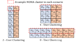
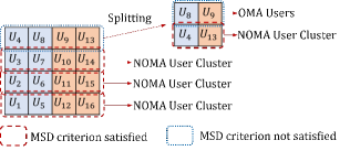
In the AMUC algorithm, whenever the $G$ users in a cluster fail to meet $\zeta_{i-1,i}$ and $\Delta^{\tiny MSD}_{\tiny i-1,i}$, we split the cluster into two halves. For this new cluster of users, we again perform the criterion check as formulated in (16) and (18). If the criterion is met for all the combinations, we continue clustering those G/2G2\lx@glossaries@gls@link{main}{G}{\leavevmode G}/2 users in . Otherwise, we continue splitting this cluster again into two new halves. We continue this procedure until we end up with a single user. If the criterion is not met for any user clustering, then that single user will be designated as user. Further, while splitting a cluster into two halves, we follow the Near-Far (NF) [NearFar2] user pairing procedure. Otherwise, the throughput gains will not be achieved. In Fig. 3, we have presented an example of splitting a 4-user cluster into two 2-user clusters. Note that the 2 users clustered together after the splitting process in Fig. 3 are exactly the same as they would have been in the case of 2-user clustering in Fig. 2.

The complexity of the proposed algorithm is calculated as follows. For each of $N/G$ clusters, the proposed algorithm initially checks (16) and (18) criterion for $(G-1)$ combinations. If the conditions are not satisfied, then it splits the cluster into two halves and checks the criterions again. This results into additionally $4\times((G/2)-1)$ computations. This procedure is continued till only one user is left in a cluster. Thus, in a worst case scenario, the complexity of the proposed AMUC algorithm is $\mathcal{O}\Big{(}(2N/G)\big{(}G\log_{2}G-((1-G)/(1-\log_{2}G))\big{)}\Big{)}$. Next, we propose the power allocation algorithm for a given set of clustered users.

Refer to caption
Figure 4: CDF of cell spectral efficiency with varying number of users in each cluster and perfect (β=0)β0(\lx@glossaries@gls@link{main}{beta}{\leavevmode\beta}=0).

IV-C Power Allocation

Based on the lower bound formulated in (9), we allocate the minimum power required for each user as follows

αi=αiabsent\displaystyle\lx@glossaries@gls@link{main}{alphai}{\leavevmode\alpha_{i}}= (1+(1j=i+1Gαj)γiOMA)χG(γiOMA).11superscriptsubscript𝑗𝑖1Gsubscript𝛼𝑗γiOMAχGγiOMA\displaystyle\Big{(}{1+\big{(}1-\sum_{j=i+1}^{\lx@glossaries@gls@link{main}{G}{\leavevmode G}}\alpha_{j}\big{)}\lx@glossaries@gls@link{main}{GammaOMA}{\leavevmode\gamma_{i}^{\text{\tiny OMA}}}}\Big{)}\lx@glossaries@gls@link{main}{Ffun}{\leavevmode\chi_{\text{\tiny G}}}(\lx@glossaries@gls@link{main}{GammaOMA}{\leavevmode\gamma_{i}^{\text{\tiny OMA}}}).

We begin allocation with user $G$, as $\alpha_{\text{\tiny G}}$ is dependent only on $\gamma^{\text{\tiny OMA}}_{\text{\tiny G}}$. We then use this allocated power $\alpha_{\text{\tiny G}}$ and $\gamma^{\text{\tiny OMA}}_{\text{\tiny G}-1}$ to recursively compute the power allocation factor $\alpha_{\text{\tiny G}-1}$. Likewise, we continue allocation till $\alpha_{\text{\tiny 1}}$. Further, when we allocate the minimum power required for each user based on (9), $\sum_{i=1}^{G}\alpha_{i}$ is less than 1. Hence, to maximize the achievable sum rates, we allocate the remaining power (1i=1G)Pt1superscriptsubscript𝑖1𝐺Pt\big{(}1-\sum_{i=1}^{G}\big{)}\lx@glossaries@gls@link{main}{Pt}{\leavevmode P_{t}} to the strong user.

We have presented a pseudo-code to implement the proposed MUC, AMUC, and power allocation in Algorithm 1. Next, we present the simulation results.

V Results and Discussion

Refer to caption
Figure 5: Mean cell spectral efficiency comparison with varying number of users in each cluster.

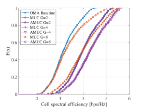
For the evaluation of the proposed algorithms, we have considered Poisson point distributed s and users with densities 25 BS/km2 and 2000 users/km2, respectively. The simulation parameters and the path loss model considered for the evaluation are as per the urban cellular scenario presented in [38901]. For each user, we calculate the received from each and then associate the user to the from which it receives maximum . We then randomly pick $N=64$ users associated with each and perform evaluation for user clusterings with $G\in\{2,\ldots,32\}$. For each $G$ value, we perform the proposed user clustering, MUC, AMUC, and power allocation as mentioned in Algorithm 1. We then perform Monte-Carlo simulations to calculate the cell spectral efficiency for each algorithm.

In Fig. 4, we plot of cell spectral efficiency for varying number of users in each cluster and for perfect (β=0)β0(\lx@glossaries@gls@link{main}{beta}{\leavevmode\beta}=0). The performance of the

Conversion to HTML had a Fatal error and exited abruptly. This document may be truncated or damaged.