A Rapid and Large-Amplitude X-ray Dimming Event in a $z\approx 2.6$ Radio-Quiet Quasar

Abstract

We report a dramatic fast X-ray dimming event in a $z=2.627$ radio-quiet type 1 quasar, which has an estimated supermassive black hole (SMBH) mass of $6.3\times 10^{9}M_{\odot}$. In the high X-ray state, it showed a typical level of X-ray emission relative to its UV/optical emission. Then its 0.5–2 keV (rest-frame 1.8–7.3 keV) flux dropped by a factor of $\approx 7.6$ within two rest-frame days. The dimming is associated with spectral hardening, as the 2–7 keV (rest-frame 7.3–25.4 keV) flux dropped by only $17\%$ and the effective power-law photon index of the X-ray spectrum changed from $\approx 2.3$ to $\approx 0.9$. The quasar has an infrared (IR)-to-UV spectral energy distribution and a rest-frame UV spectrum similar to those of typical quasars, and it does not show any significant long-term variability in the IR and UV/optical bands. Such an extremely fast and large-amplitude X-ray variability event has not been reported before in luminous quasars with such massive SMBHs. The X-ray dimming is best explained by a fast-moving absorber crossing the line of sight and fully covering the X-ray emitting corona. Adopting a conservatively small size of $5{G}M_{\rm BH}/c^{2}$ for the X-ray corona, the transverse velocity of the absorber is estimated to be $\approx 0.9c$. The quasar is likely accreting with a high or even super-Eddington accretion rate, and the high-velocity X-ray absorber is probably related to a powerful accretion-disk wind. Such an energetic wind may eventually evolve into a massive galactic-scale outflow, providing efficient feedback to the host galaxy.

1 INTRODUCTION

Active galactic nuclei (AGNs) are powered by accretion onto supermassive black holes (SMBHs) in galaxy centers, and they are characterized by luminous radiation plus emission variability across the electromagnetic spectrum. AGN multiwavelength variability may involve various physical processes, and observations of these have provided useful insights into the still elusive SMBH accretion physics. With the accumulation of astronomical data over long time spans, novel types of AGN-related variability phenomena are being discovered; e.g., the “changing-look” quasars (e.g., LaMassa et al., 2015) and the X-ray quasi-periodic eruptions (e.g., Miniutti et al., 2019; Arcodia et al., 2021).

Among the multiwavelength variability of radio-quiet AGNs (without strong jets), X-ray variability generally occurs on the shortest timescales (e.g., Ulrich et al. 1997), indicating an origin close to the central SMBH. AGN X-ray emission is considered to originate from the hot corona surrounding the inner accretion disk in the immediate vicinity of the SMBH (e.g., Gilfanov & Merloni, 2014; Fabian et al., 2017). The typical size of the corona is constrained to be around $10r_{\rm g}$, where $r_{\rm g}={G}M_{\rm BH}/c^{2}$ is the gravitational radius with $M_{\rm BH}$ being the SMBH mass, from studies of rapid X-ray variability and X-ray microlensing of AGNs (e.g., Dai et al., 2010; Morgan et al., 2012; Shemmer et al., 2014; Reis & Miller, 2013; Fabian et al., 2015). Therefore, the shortest X-ray variability timescale apparently has a SMBH-mass dependence; it is down to minutes in moderate-luminosity AGNs with $M_{\rm BH}\sim 10^{6\textrm{--}7}M_{\odot}$ (e.g., IRAS $13224-3809$; Fabian et al. 2013), and it is around hours in luminous quasars with $M_{\rm BH}\gtrsim 10^{8}M_{\odot}$ (e.g., PHL 1092; Brandt et al. 1999; Miniutti et al. 2012).

Radio-quiet AGNs also vary most strongly at X-ray energies in general. The X-ray variability amplitude (here parameterized as the fractional flux change) has a broad range. The average variability amplitude is $\approx 20\textrm{--}50\%$ for typical AGN samples, and amplitudes exceeding $\approx 2$ are rare (e.g., Gibson & Brandt, 2012; Yang et al., 2016; Maughan & Reiprich, 2019; Timlin et al., 2020). However, for individual AGNs, larger amplitude variability events have been observed with X-ray fluxes changing by factors of up to a few hundreds. For such objects, the X-ray flux may vary strongly with an amplitude of $\approx 2$ on the shortest timescales mentioned above (minutes to hours), and the amplitude generally increases with the timescale probed, reaching a maximum on year timescales.

There are a number of physical interpretations for the broad range of AGN X-ray variability. The small amplitude variability among typical AGNs is generally attributed to small fluctuations of the coronal properties (e.g., energy dissipation from magnetic flares or variation of the optical depth; Ulrich et al. 1997). The strong (amplitudes $\gtrsim 2$) or extreme (amplitudes $\gtrsim 10$) variability events are much rarer, and they call for significant changes of the coronal properties including, for example, the global accretion rate (e.g., changing-look AGNs and tidal disruption events) and the height of the corona to the SMBH (affecting the relativistic light bending and reflection effects; e.g., Ross & Fabian 2005; Fabian et al. 2012; Dauser et al. 2016). Alternatively, the strong or extreme variability might not be intrinsic to the corona but instead be due to obscuration of the coronal X-ray emission by a varying (e.g., covering factor, column density, or ionization state) X-ray absorber along the line of sight. These internal and external mechanisms are not exclusive; in some cases, changes of the coronal properties and X-ray obscuration are both invoked to explain the observed X-ray variability (e.g., Boller et al., 2021). Due to the often limited quality of AGN X-ray data and the complicated SMBH accretion physics, we still lack good understanding of the physical processes responsible for their X-ray variability.

There is a special type of X-ray variability that has attracted much attention recently (e.g., Miniutti et al., 2012; Liu et al., 2019; Ni et al., 2020; Timlin et al., 2020; Boller et al., 2021; Liu et al., 2021). Besides the strong (and often extreme) variability amplitudes, a characteristic property is that these events are found in type 1 AGNs including luminous quasars and there is no contemporaneous UV/optical continuum or emission-line variability. Empirically, there is a significant correlation observed between the UV/optical emission and X-ray emission in typical AGNs that is interpreted as an intrinsic accretion disk-corona connection and is often parameterized as a negative relation between the monochromatic luminosity at $2500~{}\textup{\AA}$ ($L_{2500~{}\textup{\AA}}$) and the X-ray-to-optical power-law slope parameter ($\alpha_{\rm OX}$) or a positive $L_{2500~{}\textup{\AA}}$–$L_{\rm 2~{}keV}$ relation (e.g., Strateva et al., 2005; Steffen et al., 2006; Gibson et al., 2008; Lusso et al., 2010; Lusso & Risaliti, 2016; Risaliti & Lusso, 2019; Liu et al., 2021). Therefore, from the stable UV/optical emission, one could infer that the intrinsic coronal X-ray emission should not change significantly. Interestingly, the available $\alpha_{\rm OX}$ values computed in the highest X-ray states of these AGNs all follow the $\alpha_{\rm OX}\textrm{--}L_{2500~{}\textup{\AA}}$ relation within the scatter (e.g., Miniutti et al., 2012; Liu et al., 2019; Ni et al., 2020; Boller et al., 2021; Liu et al., 2021), and they became smaller (more negative; representing X-ray weakness) in the other states. Thus these AGNs likely vary between the X-ray nominal-strength state and multiple X-ray weak states, arguing for the X-ray obscuration scenario where the coronal X-ray emission does not change and the observed X-ray emission is simply modified by various amounts of absorption from a small-scale dust-free X-ray absorber. These AGNs are generally considered to have high or even super-Eddington accretion rates, and the X-ray absorber is probably related to accretion-disk winds and/or thick inner accretion disks (e.g., Miniutti et al., 2012; Liu et al., 2019; Ni et al., 2020; Boller et al., 2021).

In this paper, we report a dramatic fast X-ray dimming event in a $z=2.627$ radio-quiet type 1 quasar, SDSS J$135058.12+261855.2$ (hereafter SDSS J$1350+2618$). Its coordinates are $\alpha_{\rm J2000.0}=13^{\rm h}50^{\rm m}58\fs 12$ and $\delta_{\rm J2000.0}=+26\arcdeg 18\arcmin 55\farcs 3$. We describe the basic properties of this quasar and the X-ray data analysis in Section 2. The exceptional X-ray variability is presented in Section 3. We show the spectral energy distribution (SED), infrared (IR)-to-UV light curves, and rest-frame UV spectra in Section 4. In Section 5, we discuss physical interpretation of the extreme X-ray variability and its implications. We summarize in Section 6. Throughout this paper, we adopt a flat $\Lambda$CDM cosmology with the current Planck cosmological parameters (Planck Collaboration et al., 2020) of $H_{\rm 0}=67.4~{}\rm km~{}s^{-1}~{}Mpc^{-1}$, $\Omega_{\rm M}=0.315$, and $\Omega_{\Lambda}=0.685$.

2 X-ray data analysis

SDSS J$1350+2618$ is a high-redshift ($z=2.627$; Hewett & Wild 2010) quasar recently identified as an unusual quasar that showed significantly weaker X-ray emission compared to the expectation from the $\alpha_{\rm OX}\textrm{--}L_{2500~{}\textup{\AA}}$ relation (Pu et al., 2020). It is very luminous, with an absolute $i$-band magnitude (normalized at $z=2$) of $-27.79$, and it has a C iv-based virial SMBH mass estimate of $6.3\times 10^{9}M_{\odot}$ (Shen et al., 2011). Upon detailed investigation, we found that this quasar has been serendipitously observed three times by Chandra. It displayed strong X-ray variability, and there was also a state where it showed a nominal level of X-ray emission. The Chandra observations and the derived X-ray photometric properties are listed in Table 1, and the data-analysis procedure is described in the following.

SDSS J$1350+2618$ was serendipitously observed three times by Chandra ACIS-I during Cycle 18 (observation IDs: 17627, 17621, 17222). The primary targets of these three Chandra observations are the outskirts of a galaxy cluster, Abell 1795. SDSS J$1350+2618$ is $\approx 33\arcmin$ away from the cluster center, and thus its X-ray data are not contaminated by the diffuse X-ray emission of the cluster. The off-axis angles of SDSS J$1350+2618$ in the three observations are 6.4′, 2.6′, and 6.7′, respectively. SDSS J$1350+2618$ landed on the ACIS-I CCD gap in the second observation, and thus its effective exposure time in this observation is the lowest among the three despite the longest total exposure time and smallest off-axis angle. The CCD gap effects were accounted for by the effective exposure time and the spectral response files used in the following photometric and spectroscopic analyses.

We analyzed the Chandra data using the Chandra Interactive Analysis of Observations (CIAO; v4.11) tools. For each observation, we first ran the chandra_repro script to generate a new level 2 event file, and then filtered high-background flares using the deflare script with an iterative $3\sigma$ clipping algorithm; only $\approx 1\%$ of the total exposure was excluded. From the cleaned level 2 event file, images in the soft (0.5–2 keV), hard (2–7 keV), and full (0.5–7 keV) bands were generated using the dmcopy tool. We then ran the automated source-detection tool wavdetect (Freeman et al., 2002) to search for X-ray sources in the three images, with a false-positive probability threshold of $10^{-6}$ and wavelet scale sizes of 1, 1.414, 2, 2.828, 4, 5.656, and 8 pixels. We matched X-ray positions of the detected sources in each image to the optical position of SDSS J$1350+2618$. If the optical position of SDSS J$1350+2618$ was matched within 2″ of an X-ray position, we considered SDSS J$1350+2618$ detected by wavdetect and adopted the X-ray position as the source position to perform aperture photometry. Otherwise, the optical position was adopted. For the first observation, SDSS J$1350+2618$ was not detected by wavdetect in any bands. For the second observation, it was detected in all three bands. For the third observation, it was detected in the hard and full bands, but not in the soft band.

The Chandra point-spread function (PSF) varies with energy as well as off-axis angle, and the off-axis PSF shape is approximately an ellipse. In order to minimize the number of background counts enclosed by the source extraction region and obtain a maximum signal-to-noise ratio, we used an elliptical region as the source aperture, which was determined with the following procedure. For each of the three images in each observation, we simulated an X-ray source at the SDSS J$1350+2618$ position on the CCD chip, using the Chandra Ray Tracer (ChaRT; Carter et al. 2003) and Model of AXAF Response to X-rays (MARX; Davis et al. 2012) software suites. ChaRT was first run to trace rays through the Chandra X-ray optics, using the source coordinates, an assumed $\Gamma=2$ power-law spectrum, and the observation ID as inputs. The collected rays were projected to the detector plane via MARX, taking into account all detector effects. An image that consists of the simulated photons was thus created. The dmellipse tool was then used to determine an elliptical region that encloses 85%–94% of the simulated photon flux; the elliptical size and the corresponding encircled-energy fraction (EEF) were chosen so that we can obtain the maximum signal-to-noise ratio for the source in the real image. The soft- and hard-band images with the source extraction regions are shown in Figure 1.

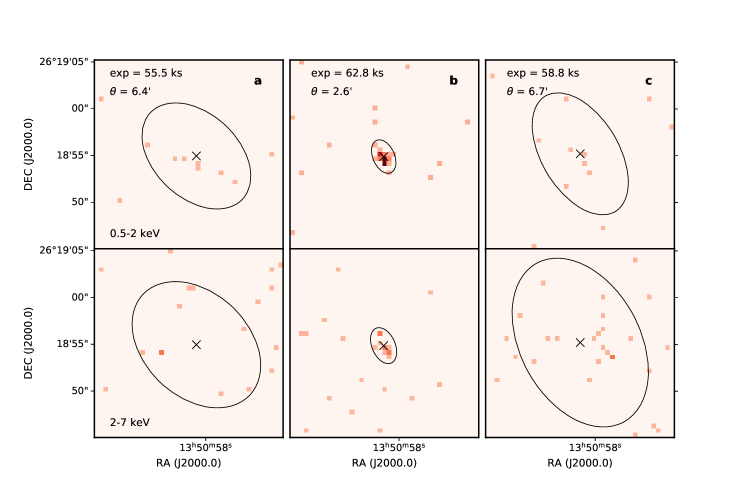
Figure 1: Chandra 0.5–2 keV (upper panel) and 2–7 keV (lower panel) images of the three observations for SDSS J$1350+2618$. The observational dates are a 2015 Aug 28, b 2016 Mar 27, and c 2016 Apr 3. The ellipse in each image is the source extraction region used for aperture photometry. The aperture sizes are chosen so that the signal-to-noise ratios are the largest. For observations a and c, the encircled-energy fractions (EEFs) of the source apertures are all 94%; for observation b, the EEF is 90% (85%) for the soft (hard) band. The total exposure time and off-axis angle ($\theta$) of each observation are noted in each of the 0.5–2 keV images.

We extracted source counts ($S$) from the elliptical region determined above. Background counts ($B$) were extracted from an annulus region centered on the source position with a 10″ inner radius and a 50″ outer radius. We have verified that there is no source detected by wavdetect in any of the background regions. We then assessed the source-detection significance via computing the binomial no-source probability (e.g., Luo et al., 2015; Liu et al., 2018), $P_{\rm B}$, with the expression:

$$P_{\rm B}=\sum_{X=S}^{N}\frac{N!}{X!(N-X)!}p^{X}(1-p)^{N-X}~{},$$ (1)

where $N$ is the total number of raw source and background counts ($=S+B$), and $p=1/(1+BACKSCAL)$ with $BACKSCAL$ being the ratio between the areas of the background and source regions. The computed $P_{\rm B}$ values are all smaller than $0.01$, corresponding to $>2.6\sigma$ detection significance levels. SDSS J$1350+2618$ is thus considered to be detected in every image for the following photometric analysis. We calculated $1\sigma$ errors of the source and background counts following the Poisson approach of Gehrels (1986), and errors of the net counts were propagated from the errors of the source and background counts. The net counts and associated errors in the soft and hard bands are listed in Table 1.

We derived an effective photon index ($\Gamma_{\rm eff}$) for a power-law spectrum from the observed band ratio, defined as the ratio of the hard-band to soft-band counts, following a procedure similar to that in Liu et al. (2018). For each observation, we used the fakeit routine in XSPEC (v12.10.1; Arnaud 1996) to generate a set of simulated spectra based on the response matrices and ancillary response functions in the source-extraction regions of the soft- and hard-band images, where a Galactic absorption ($N_{\rm H}=1.12\times 10^{20}~{}\rm cm^{-2}$; HI4PI Collaboration et al. 2016) modified power-law model with a set of $\Gamma$ values was assumed. We then calculated the corresponding band ratio from the simulated spectra for each of the assumed $\Gamma$ value. The $\Gamma_{\rm eff}$ values were then derived from the observed band ratios by interpolating the $\Gamma$–band ratio sets. The associated $1\sigma$ errors were propagated from the $1\sigma$ errors of the observed band ratios that were computed using the Bayesian code BEHR (Park et al., 2006). For each energy band, we converted the observed source count rate to flux, with a conversion factor derived from the simulated spectrum with photon index $\Gamma_{\rm eff}$. The flux errors were propagated from the errors of the net counts. Table 1 lists the $\Gamma_{\rm eff}$ and flux values.

We also extracted the spectrum of the second observation and performed spectral fitting using XSPEC. The source spectrum was extracted from an elliptical region with an EEF of $90\%$ in the full band, and the background spectrum was extracted from the same annulus region used in the aperture photometry described above. The source spectrum was grouped with at least one count per bin. We fitted the 0.5–7 keV spectrum with a power-law model modified by the Galactic absorption (phabs*zpowerlw), and the W statistic was used in parameter estimation. The best-fit photon index is $2.1\pm 0.4$, consistent with the $\Gamma_{\rm eff}$ value within the uncertainties. The model-predicted fluxes in the soft and hard bands are also consistent with those obtained from the photometric analysis.

3 X-ray variability

The strong X-ray variability of SDSS J$1350+2618$ is evident from the soft-band fluxes listed in Table 1. The 0.5–2 keV (rest-frame 1.8–7.3 keV) flux of the second observation is larger than that of the first observation by a factor of $6.0_{-2.6}^{+4.6}$, and it is larger than that of the third observation by a factor of $7.6_{-3.4}^{+6.9}$. The 1$\sigma$ uncertainties of these variability factors were propagated from the flux uncertainties following the method described in Section 1.7.3 of Lyons (1991). On the other hand, the flux variability is much weaker in the hard band (rest-frame 7.3–25.4 keV). The hard-band flux of the second observation is only higher than those of the first and third observations by factors of $1.8_{-0.9}^{+2.0}$ and $1.2_{-0.5}^{+0.9}$, respectively. Considering the uncertainties, these hard-band fluxes are actually consistent with each other. The significantly different variability amplitudes in the soft and hard bands imply that there is variability in the X-ray spectral shape, which is also indicated by the $\Gamma_{\rm eff}$ values in Table 1. SDSS J$1350+2618$ exhibits a steep spectral shape in the second observation ($\Gamma_{\rm eff}=2.3\pm 0.4$), while the spectra appear flatter in the other two observations, with $\Gamma_{\rm eff}$ values of $1.4^{+0.9}_{-0.7}$ and $0.9^{+0.7}_{-0.6}$, respectively.

We further quantify the X-ray variability using the $\alpha_{\rm OX}$ parameter, which allows us to assess the deviations of the levels of the observed X-ray emission from the nominal level expected from the $\alpha_{\rm OX}\textrm{--}L_{2500~{}\textup{\AA}}$ relation. We used the soft-band fluxes to derive the flux densities at rest-frame 2 keV, assuming a power-law model with the measured $\Gamma_{\rm eff}$ values. The $2500~{}\textup{\AA}$ flux density was determined through interpolation of the photometric data from the Sloan Digital Sky Survey (SDSS) (York et al., 2000), which is consistent with the value provided by Shen et al. (2011). We note that although the X-ray and SDSS observations are not simultaneous, there does not appear to be any significant UV/optical variability (see Section 4 below) that could bias the $\alpha_{\rm OX}$ measurements. The derived $\alpha_{\rm OX}$ values are listed in Table 1. We then calculated the differences ($\Delta\alpha_{\rm OX}$) between the observed $\alpha_{\rm OX}$ values and those expected from the $\alpha_{\rm OX}\textrm{--}L_{2500~{}\textup{\AA}}$ relation in Steffen et al. (2006), and the results are also listed in Table 1. SDSS J$1350+2618$ showed nominal-strength X-ray emission in the second observation, with $\Delta\alpha_{\rm OX}=0.03$, while it showed weak X-ray emission in the first and third observations, by factors of $8.7^{+6.3}_{-3.4}$ and $16.8^{+14.7}_{-6.7}$ ($10^{-\frac{\Delta\alpha_{\rm OX}}{0.3838}}$ with the 1$\sigma$ uncertainties propagated from the flux uncertainties), respectively. These X-ray weakness factors (based on the 2 keV flux densities) differ from the 0.5–2 keV flux variability amplitudes computed above ($\approx 6.0$ and $7.6$), mainly due to different $\Gamma_{\rm eff}$ values of the three observations which were used to convert fluxes to flux densities.

Therefore, SDSS J$1350+2618$ exhibited faint X-ray emission in 2015 August, with a rest-frame 2 keV flux density $\approx 8.7$ times weaker compared to the expectation from its UV/optical flux. In 2016 March (two months later in the quasar rest frame), the second Chandra observation revealed that the quasar recovered to an X-ray nominal-strength state. The third observation in 2016 April ($47.2$ hours later in the rest frame) surprisingly showed that the quasar had dimmed by a factor of $\approx 7.6$ in terms of its 0.5–2 keV (rest-frame 1.8–7.3 keV) flux. The dimming is associated with spectral hardening, as the 2–7 keV (rest-frame 7.3–25.4 keV) flux dropped by only $17\%$. The effective power-law photon index ($\Gamma_{\rm eff}$) of the X-ray spectrum changed from $2.3\pm 0.4$ to $0.9_{-0.6}^{+0.7}$. The most remarkable finding here is the extremely fast X-ray dimming from an X-ray nominal-strength state to a significantly X-ray weak state within two rest-frame days, which has never been observed before among luminous quasars with such massive SMBHs.

4 Spectral energy distribution and multiwavelength properties

We explored if SDSS J$1350+2618$ displays any unusual features in its multiwavelength data. We collected IR-to-UV photometric data for SDSS J$1350+2618$, in order to construct its SED and explore if there is notable variability in the IR-to-UV bands. The data were collected from the public catalogs of the Wide-field Infrared Survey Explorer (WISE; Wright et al. 2010), Near-Earth Object WISE Reactivation (NEOWISE; Mainzer et al. 2014), UKIRT Infrared Deep Sky Survey (UKIDSS; Lawrence et al. 2007), Pan-STARRS1 Surveys (PS1; Chambers et al. 2016), SDSS, Zwicky Transient Facility (ZTF; Bellm et al. 2019), and Catalina Real-Time Transient Survey (CRTS; Drake et al. 2009). All the data were corrected for Galactic extinction ($E_{\rm B-V}=0.0122$; Schlegel et al. 1998) using the extinction law of Cardelli et al. (1989). Except for the UKIDSS and SDSS catalogs that provide only single-epoch measurements and the WISE catalog that has stacked measurements, the other surveys provide multiple measurements from long-term multi-epoch observations, and we used their error-weighted average measurements to construct the SED, shown in Figure 2. Particularly, for the NEOWISE data, we plotted the average measurements in the day closest to the third Chandra observation. For the X-ray SED, we derived the 2 keV and 10 keV luminosities from the 0.5–2 keV and 2–7 keV fluxes, adopting a power-law model with the $\Gamma_{\rm eff}$ values from the aperture photometry. For comparison, the mean SED of SDSS quasars in Krawczyk et al. (2013) is also shown, which is scaled to the mean $2500~{}{\textup{\AA}}$ luminosity of SDSS J$1350+2618$ interpolated from the SDSS photometric data. Except for the stronger mid-IR emission, SDSS J$1350+2618$ shows a fairly typical quasar IR-to-UV SED. The strong X-ray variability is clearly visible in the SED plot, which also indicates that SDSS J$1350+2618$ was in an X-ray nominal-strength state during the second observation with a steep spectral shape, and it switched to X-ray weak states in the first and third observations with flatter spectral shapes.

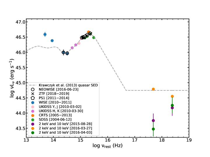
Figure 2: IR-to-X-ray SED for SDSS J$1350+2618$. The IR-to-UV data points were gathered from the WISE, NEOWISE, UKIDSS, PS1, SDSS, ZTF, and CRTS catalogs, where the WISE, PS1, ZTF, and CRTS data points show the average measurements of multi-epoch observations. The rest-frame 2 keV and 10 keV luminosities for the three Chandra observations were derived from the observed 0.5–2 keV and 2–7 keV fluxes, adopting a power-law model with the measured $\Gamma_{\rm eff}$ values. The corresponding observational dates/periods are listed in the lower left corner. The data error bars show $1\sigma$ uncertainties, and some of them are smaller than the symbol size. The dashed curve shows the mean SED of SDSS quasars in Krawczyk et al. (2013), which is scaled to the $2500~{}{\textup{\AA}}$ luminosity of SDSS J$1350+2618$ interpolated from the SDSS photometric data. Except for the stronger mid-IR emission, SDSS J$1350+2618$ shows an IR-to-UV SED consistent with the mean quasar SED.

Through integrating the scaled $1\rm~{}\mu m\textrm{--}10$ keV mean quasar SED shown in Figure 2, we estimate a bolometric luminosity ($L_{\rm Bol}$) of $1.3\times 10^{47}$ erg s^-1 for SDSS J$1350+2618$. With the Eddington luminosity computed as $L_{\rm Edd}=1.26\times 10^{38}M_{\rm BH}$ erg s^-1, the Eddington ratio ($L_{\rm Bol}/L_{\rm Edd}$) of this quasar is $\approx 0.16$, consistent with the value provided in Shen et al. (2011). This Eddington ratio is within the interquartile range of $\approx 0.15\textrm{--}0.46$ for the Eddington ratios of typical quasars at $z=2\textrm{--}3$ (Shen et al. 2011), suggesting that the SMBH mass estimate for SDSS J$1350+2618$, although uncertain, is not off by a large factor. Its large X-ray photon index of $2.3\pm 0.4$ in the X-ray nominal-strength state also suggests that SDSS J$1350+2618$ is accreting with a high or even super-Eddington accretion rate (e.g., Shemmer et al., 2008).

We then constructed IR-to-UV light curves obtained from the PS1, ZTF, CRTS, and NEOWISE catalogs, shown in Figure 3. For the ZTF, CRTS, and NEOWISE light curves, we grouped any intra-day measurements. In the PS1 light curves, we also included the SDSS $g$-, $r$-, $i$-, $z$-band photometric measurements and the $g$-, $r$-, $i$-band magnitudes derived from the SDSS spectrum. In the CRTS light curve, we added the $V$-band magnitude derived from the SDSS spectrum, of which the observational date overlaps the CRTS light curve. These light curves indicate that SDSS J$1350+2618$ does not show any substantial long-term variability in the IR and UV/optical bands. Although only the NEOWISE light curve overlaps the X-ray observational dates, the mild variability with amplitudes $\lesssim 1.5$ ($\approx 0.4$ mag) in all the rest-frame IR-to-UV bands shown in Figure 3 indicates that there were unlikely any significant changes of the accretion power. Thus, the $\alpha_{\rm OX}$ values and X-ray states (nominal-strength state for the second observation and weak states for the first and third observations) of SDSS J$1350+2618$, determined using the non-simultaneous X-ray and SDSS photometric (for $f_{2500~{}\textup{\AA}}$ interpolation) data, should not be affected by any potential strong UV variability.

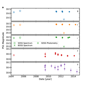
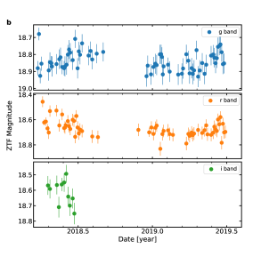
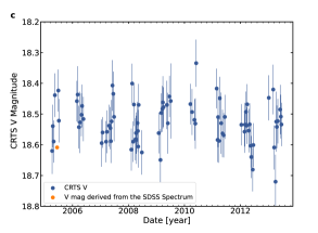
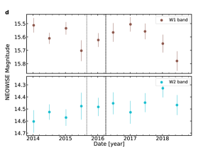
Figure 3: IR-to-UV light curves. a, PS1 $g$, $r$, $i$, $z$, and $y$ bands. b, ZTF $g$, $r$, and $i$ bands. c, CRTS $V$ band. d, NEOWISE W1 and W2 bands. For the ZTF, CRTS, and NEOWISE light curves, we grouped any intra-day measurements. In the PS1 light curves, we also included the SDSS $g$-, $r$-, $i$-, $z$-band photometric measurements and the $g$-, $r$-, $i$-band magnitudes derived from the SDSS and BOSS spectra. The BOSS measurements are likely incorrect, probably due to absolute flux calibration issues. In the CRTS light curve, we added the $V$-band magnitude derived from the SDSS spectrum. In the NEOWISE light curve, the three vertical dashed lines indicate the observational dates of the X-ray observations. These light curves indicate that SDSS J$1350+2618$ does not show any substantial long-term variability in the IR and UV/optical bands.

The SDSS spectrum taken in 2005 is displayed in Figure 4. The spectrum has been corrected for the Galactic extinction. For comparison, the composite spectrum of SDSS quasars (Vanden Berk et al., 2001) was plotted with a gray curve. The continuum appears to be slightly bluer than the composite spectrum. The C iv $\lambda 1549$ and C iii] $\lambda 1909$ emission lines are weaker than those in the composite spectrum. The C iv rest-frame equivalent width is only 12.2 Å (Shen et al. 2011), compared to the 30 Å value for the composite spectrum, and thus SDSS J$1350+2618$ could be classified as a weak emission-line quasar (WLQ), a small population of type 1 quasars that show unusually weak UV emission lines. Similar to many other WLQs, SDSS J$1350+2618$ also shows a large C iv blueshift; the measurement from Shen et al. (2011) adjusted to the improved redshift (Hewett & Wild, 2010) is 2630 km s^-1. The prominent C iv blueshifts in WLQs suggest a strong wind component for the C iv broad emission-line region (BELR). There are no broad absorption features in the rest-frame UV spectrum. But there appear to be a C iv narrow absorption line (NAL) at 1413 Å and a Ly$\alpha$ NAL at 1177 Å.

Besides the SDSS spectrum, there is also a SDSS Baryon Oscillation Spectroscopic Survey (BOSS) spectrum for SDSS J$1350+2618$ taken in 2012. The BOSS spectrum, shown in Figure 4, is very similar to the SDSS spectrum with a similarly weak C iv emission line and two similar NALs, but the overall flux is lower by a factor of $\approx 3$. The ratio curve of the two spectra (Figure 4) is featureless, indicating no apparent spectral variability besides the flux difference. The $g$-, $r$-, $i$-band magnitudes derived from the BOSS spectrum were also presented in the PS1 light curves (Figure 3a) for comparison. Since there is no significant variability observed in the optical photometric light curves which cover the observational dates of the SDSS and BOSS spectra, we consider the BOSS flux measurement incorrect, probably due to some BOSS absolute flux calibration issues.

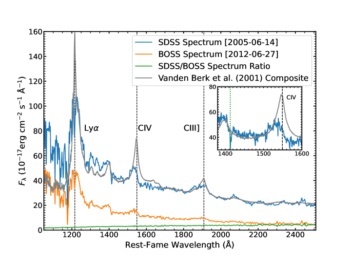
Figure 4: SDSS spectrum of SDSS J$1350+2618$ (blue curve). The inset shows a zoomed-in view of the C iv $\lambda 1549$ emission line and an associated NAL at 1413 Å. For comparison, the gray curve shows the composite spectrum of typical SDSS quasars (Vanden Berk et al., 2001), scaled to the spectrum of SDSS J$1350+2618$ at rest-frame $1695~{}\textup{\AA}$. There are no broad absorption features in the spectrum of SDSS J$1350+2618$. Compared to typical quasars, SDSS J$1350+2618$ shows a weaker and blueshifted C iv emission line. The BOSS spectrum is also displayed (orange curve), showing similar spectral features. The overall flux of the SDSS spectrum is higher than that of the BOSS spectrum by a factor of $\approx 3$, and the green curve shows the ratio of these two spectra. We consider the BOSS flux measurement unreliable, probably due to absolute flux calibration issues.

5 Discussion

We presented the extreme X-ray variability of SDSS J$1350+2618$. The rapid and large-amplitude X-ray dimming from the second observation to the third observation appears unique among such luminous quasars. Unfortunately, the limited photon statistics of the X-ray data in the third observation (with $\approx 17$ 0.5–7 keV net counts) do not allow detailed spectral modeling; we are not even able to demonstrate conclusively that absorption must be present given the flat but rather uncertain effective photon index ($0.9^{+0.7}_{-0.6}$), although the data suggest this is a likely possibility. Therefore, the nature of the dimming is not immediately clear. In the following discussion, we consider that the dimming is most naturally explained by an X-ray eclipse event, based on the X-ray and multiwavelength properties presented above and our current understanding of AGNs with similar properties, although their SMBH masses are not as large or their variability timescales are not as short. However, we do not consider this obscuration scenario conclusive. Future observations of SDSS J$1350+2618$ or discoveries of similar events should shed additional light on the elusive nature.

5.1 A Near-Light-Speed X-ray Eclipse Event

The X-ray variability of SDSS J$1350+2618$ has a few distinctive features, namely, an extremely short timescale of $\approx$ 2 days for a $M_{\rm BH}\approx 6.3\times 10^{9}M_{\odot}$ SMBH, variation between X-ray normal and significantly X-ray weak states, and a typical photon index of $\approx 2.3$ in the X-ray nominal-strength state and spectral hardening in the X-ray weak states. These features immediately suggest varying X-ray obscuration as the most natural physical interpretation for the variability. The short variability timescale does not permit any significant changes to the accretion rate, and thus the scenarios of changing-look events or TDEs can be excluded; the typical quasar IR-to-UV SED and the lack of significant IR-to-UV long-term variability also argue against these scenarios. Besides X-ray obscuration, the other scenario that can modify the observed X-ray emission is the relativistic disk-reflection model (e.g., Ross & Fabian, 2005; Fabian et al., 2012; Dauser et al., 2016). In this case, the weak X-ray emission is due to the light bending effects when the corona moves very close to the SMBH, and the observed spectrum is dominated by a disk-reflected component; the X-ray variability is due to changes of the corona height/size which affect the strengths of the light bending and disk-reflection effects. However, for SDSS J$1350+2618$, the hard-band (rest-frame 7.3–25.4 keV) flux in the third observation dropped by only 17% compared to the X-ray nominal-strength state in the second observation that has a typical unobscured power-law spectrum; this cannot be produced by a disk-reflected spectrum which should be much weaker than the intrinsic spectrum in the hard band.

Therefore, a change of X-ray obscuration remains the only viable scenario. Indeed, the changes of X-ray fluxes and spectral shape from the second to the third observation are all consistent with change from an unobscured spectrum to a heavily obscured spectrum. A schematic illustration of the obscuration scenario in displayed in Figure 5. Under this scenario, the transverse velocity of the absorber can be constrained. Given the occultation time of $47.2$ hours between the second and third observations, and adopting a conservatively small size of $5r_{\rm g}$ for the X-ray corona, the velocity of the absorber reaches a relativistic value of $\approx 0.9c$. Uncertainty of this unprecedentedly high velocity constraint mainly comes from the uncertain SMBH mass estimate, as there is no reliable method for measuring SMBH masses of high-redshift quasars. Nevertheless, the extreme X-ray flux and spectral-shape variability of SDSS J$1350+2618$ suggest a novel eclipse event in the vicinity of a massive SMBH.

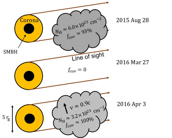
Figure 5: A schematic diagram of the varying X-ray obscuration in SDSS J$1350+2618$. The moving gas clumps with different sizes and column densities sometimes cross the line of sight and partially shield the X-ray corona. During the first X-ray observation (2015 Aug 28), the corona of SDSS J$1350+2618$ was partially covered by a clump with a covering factor of $\approx 93\%$ and a column density of $\approx 6.0\times 10^{23}\ \rm cm^{-2}$. The corona was not covered by any clumps in the second observation (2016 Mar 27). Within two rest-frame days, a fast-moving clump with a column density of $\approx 3.2\times 10^{23}\ \rm cm^{-2}$ crossed the line of sight to the corona, and it fully ($\approx 100\%$) covered the corona in the third observation. The X-ray absorber is probably not a large cloud as shown in the cartoon but instead a combination of small gas clumps. The column densities of the clumps are estimated from our assumed model and are thus model dependent (Section 5.1). Given the crossing time of $47.2$ hours and assuming a corona size of $5r_{\rm g}$ (corresponding to the minimum transverse traveling distance of the clump), the transverse velocity of this clump is estimated to be $\approx 0.9c$. Uncertainty of this unprecedentedly high velocity constraint mainly comes from the uncertain SMBH mass estimate.

We then tried to constrain the properties of the X-ray absorber by fitting the X-ray spectra in the first and third observations with a partial-covering absorption model. We note that this approach was not to analyze the X-ray data, which was presented in Section 2. Instead, we were simply trying to derive basic physical constraints under our inferred obscuration scenario. The spectra in the first and third observations are not of high quality for complex spectral modeling, and thus we had to fix most of the spectral parameters at assumed/inferred values. The extraction and simple power-law fitting of the spectrum in the second observation are described in Section 2. For the first and third observations, we extracted the source spectra from elliptical regions with a $95\%$ EEF in the full band and background spectra from an annulus region with an inner (outer) radius of 10″ (50″). The spectra were grouped with a minimum number of one count per bin, and the W statistic was used in parameter estimation. The overall partial-covering absorption model in XSPEC is phabs*(constant1*zpowerlw*zphabs*cabs+ constant2*zpowerlw), where phabs is to account for the Galactic absorption, constant1 is the covering factor of the intrinsic absorber, and constant2=1-constant1. The cabs component takes into account the Compton scattering of the absorber with its column density tied to that of the zphabs component. We fixed the intrinsic continuum (photon index and normalization of zpowerlw) to the best-fit power law of the second observation. We further fixed the covering factor in the third observation to $1.0$, as the flat spectral shape ($\Gamma_{\rm eff}\approx 0.9$) does not suggest a partial-covering absorber. The best-fit results are shown in Figure 6. For the first observation, the column density is $(6.0_{-2.3}^{+6.9})\times 10^{23}\ \rm cm^{-2}$ and the covering factor is $0.93_{-0.12}^{+0.07}$; for the third observation, the column density is $(3.2_{-1.0}^{+1.7})\times 10^{23}\ \rm cm^{-2}$. The quoted errors are at a 68% ($1\sigma$) confidence level for one parameter of interest. These basic absorber properties are included in the schematic illustration of the obscuration scenario in Figure 5. We caution that these parameters are derived based on our assumed model and are thus model dependent. The real absorber might be more complex (e.g., partially ionized), but the data do not allow constraints on more complicated models. Our previous argument about the absorber velocity does not rely on these absorber parameters.

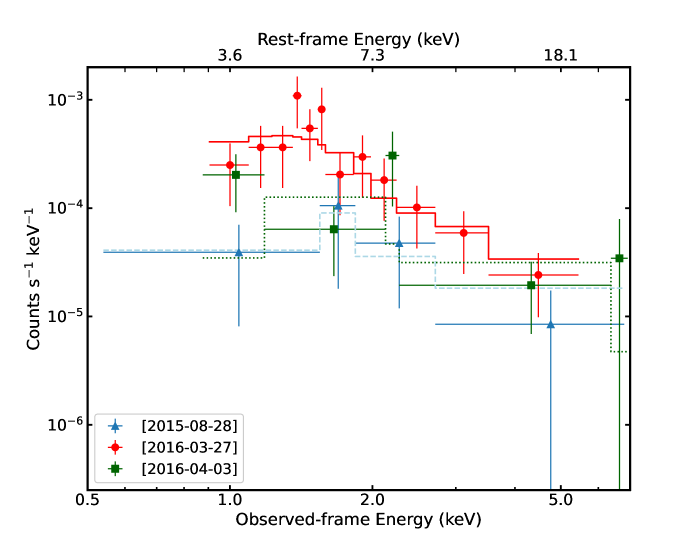
Figure 6: Three Chandra spectra overlaid with the best-fit models in the obscuration scenario. The spectra are grouped for display purposes. The spectrum of the second observation is fitted with a simple power-law model, and the best-fit spectrum is fixed as the intrinsic continuum in the partial-covering absorption modeling of the first and third observations. Basic absorber properties in the first and third observations are thus derived, as shown in Figure 5. We note that this approach was not to analyze the X-ray data, but to derive basic absorber parameters, and the results are strongly model dependent. The real absorber might be more complex (e.g., partially ionized), but the data do not allow constraints on more complicated models. Our previous argument about the absorber velocity does not rely on these absorber parameters.

5.2 Connections to Ultra-Fast Outflows and AGN Feedback

The high-velocity X-ray absorber in SDSS J$1350+2618$ is reminiscent of ultra-fast outflows (UFOs) with velocities up to $0.1\textrm{--}0.4c$ found in an increasing number of low-redshift AGNs (e.g., Tombesi et al., 2010; Gofford et al., 2013). The velocities were inferred from substantially blueshifted iron absorption lines detected in the $\gtrsim 7$ keV X-ray spectra. The UFOs are considered to be launched from the inner accretion disk since the outflow velocities are comparable to the escape velocities at small radii. The UFOs are probably clumpy, and the high-density part could provide a large amount of absorption to the X-ray continuum and thus be responsible for large-amplitude X-ray spectral variability observed in a few local AGNs (e.g., Hagino et al., 2016; Matzeu et al., 2016; Parker et al., 2018). Moreover, these UFOs may carry a large amount of mechanical power, being a possible source for AGN feedback into the host galaxy (e.g., Crenshaw & Kraemer, 2012; King & Pounds, 2015). Although UFOs are becoming fairly well characterized in local AGNs, there is still a lack of understanding about them in the distant universe. Since high-quality X-ray spectra are required to diagnose the presence of hard X-ray absorption lines, evidence of UFOs has been collected for only a limited number of high-redshift quasars (e.g., Chartas et al., 2002, 2003, 2007, 2016, 2021; Dadina et al., 2018).

The X-ray absorber in SDSS J$1350+2618$ may share the same origin as the UFOs. Due to the limited photon statistics of the three Chandra spectra, we cannot resolve any X-ray absorption lines or determine the ionization state of the X-ray absorber. It has been suggested that UV NALs are common in quasars with X-ray identified UFOs and these outflows are probably linked (e.g., Chartas et al., 2021). If the C iv and Ly$\alpha$ NALs of SDSS J$1350+2618$ (Section 4) are intrinsic to the quasar instead of from intervening systems, the corresponding outflow velocities are $\approx 0.09c$ and $0.03c$, respectively. Thus, these two NALs might provide additional support to the presence of the high-velocity X-ray absorber in SDSS J$1350+2618$. The partial-covering absorber that shielded the X-ray corona could be associated with denser and less-ionized clumps embedded in the inhomogeneous wind, such as those suggested in Hagino et al. (2016) and Matzeu et al. (2016). Clumpy structures are generally expected in quasar outflows due to thermal instabilities (e.g., Waters et al., 2017; Dannen et al., 2020) and/or radiation hydrodynamic instabilities (e.g., Takeuchi et al., 2014). The stochastic clumps with different sizes and densities in the fast wind move across our line of sight occasionally, resulting in the observed large-amplitude fast X-ray variability. The $\approx 0.9c$ velocity constrained above for the absorber could be related to the outflow and rotational velocities of the wind.

Under the clumpy wind scenario, the relativistic outflow in SDSS J$1350+2618$ may carry a large amount of energy and mass into the host galaxy, providing efficient AGN feedback. With the estimated properties of the X-ray absorber, the mass outflow rate can be estimated following the expression of $\dot{M}_{\rm out}=4\pi\mu rN_{\rm H}v_{\rm out}m_{\rm p}C_{g}$ (Crenshaw & Kraemer 2012), where $N_{\rm H}$ and $v_{\rm out}$ are the column density and velocity of the absorber, $r$ is the absorber’s radial location, $\mu$ is the mean atomic mass per particle ($=1.4$ for solar abundances), $m_{\rm P}$ is the proton mass, and $C_{g}$ is the global covering fraction of the outflow (assumed to be 0.5 based on the UFO absorber statistics; Crenshaw & Kraemer 2012 and references therein). We assume that $v_{\rm out}$ equals the transverse velocity ($\approx 0.9c$) of the absorber, $N_{\rm H}=3.2\times 10^{23}~{}\rm cm^{-2}$, and $r=10r_{\rm g}$ considering the high velocity of the absorber. Under these assumptions, we estimate the mass-outflow rate to be $\approx 19~{}M_{\odot}~{}{\rm yr^{-1}}$. The energy outflow rate (mechanical power) can thus be estimated to be $\dot{E}_{\rm out}=\frac{1}{2}\dot{M}_{\rm out}v_{\rm out}^{2}\approx 4.3\times 10^{47}~{}\rm erg~{}s^{-1}$. This value exceeds the bolometric luminosity ($1.3\times 10^{47}~{}\rm erg~{}\rm s^{-1}$) estimated above, and it is around $54\%$ of the Eddington luminosity of SDSS J$1350+2618$. The main uncertainty of this $\dot{E}_{\rm out}$ estimate is from the $v_{\rm out}$ (and thus SMBH mass) uncertainty. Moreover, if the quasar is indeed super-Eddington accreting, the bolometric luminosity or the Eddington luminosity is not an accurate representative of the accretion power, as a large fraction of the energy may be advected into the SMBH or be converted into the mechanical power of a wind (e.g., Jiang et al., 2019). Nevertheless, the outflow efficiency ($\dot{E}_{\rm out}/L_{\rm Bol}$) likely exceeds the threshold of $\dot{E}_{\rm out}/L_{\rm Bol}>0.5\textrm{--}5\%$ for significant feedback into the host galaxy (e.g., Di Matteo et al., 2005; Hopkins & Elvis, 2010). Such an outflow has enough power to sweep out dust and gas from the host galaxy, quenching the star formation and further SMBH growth.

5.3 Connections to Super-Eddington Accreting AGNs and WLQs

The main observational properties of SDSS J$1350+2618$, the variability between X-ray normal and X-ray weak states with no significant UV/optical variability, have already been found in a small population of AGNs including high-redshift quasars that are considered to have super-Eddington accretion rates (Section 1), although previously discovered variability timescales are not sufficiently short to constrain a relativistic outflow as in SDSS J$1350+2618$. Powerful radiatively driven accretion-disk winds are expected in these systems (e.g., Takeuchi et al., 2014; Giustini & Proga, 2019; Jiang et al., 2019), and the denser and less-ionized clumps of the winds likely provide the varying partial-covering absorption for interpreting the X-ray variability. The fraction of super-Eddington accreting AGNs showing such strong X-ray variability is poorly constrained ($\sim 15\%$; Liu et al. 2019), mainly due to the limited numbers of multi-epoch observations currently available. Inclination angle is probably a key factor determining whether we can observe (variable) X-ray absorption in these AGNs. Another important factor might be the Eddington ratio, which likely affects the strength/density and covering factor of the clumpy disk wind.

Similar to SDSS J$1350+2618$, some of these quasars are classified as WLQs with unusually weak UV high-ionization emission lines (e.g., C iv; Figure 4). Systematic studies of WLQ X-ray emission have revealed that a large fraction ($\sim 50\%$) of them are X-ray weak while the others show typical levels of X-ray emission (e.g., Luo et al., 2015; Ni et al., 2018; Pu et al., 2020; Ni et al., 2022). A few WLQs have also been found to vary between X-ray normal and X-ray weak states like SDSS J$1350+2618$ but the established variability timescales are not as short (Miniutti et al., 2012; Ni et al., 2020, 2022). The X-ray weakness and variability of the WLQs are naturally explained by the varying partial-covering absorption from the clumpy disk winds. The weak line emission is probably due to heavy shielding of the EUV/X-ray ionizing photons from reaching the C iv BELR by a thick inner accretion disk and/or its clumpy wind (e.g., Luo et al., 2015; Ni et al., 2018, 2022). Apparently, not all such X-ray variable quasars are WLQs, and this might be related to the thickness of the inner accretion disk that mainly depends on the Eddington ratio; i.e., WLQs are probably highly super-Eddington accreting with very thick disks. Unfortunately, neither the SMBH masses nor the bolometric luminosities (e.g., see discussion in Section 4.3 of Liu et al. 2021) of super-Eddington accreting quasars can be reliably estimated, and thus much work is still needed to understand the physical difference between WLQs and typical super-Eddington accreting quasars.

An alternative origin of the X-ray absorber is the thick inner accretion disk in these super-Eddington accreting AGNs, as proposed in studies of the X-ray emission from WLQ samples (Luo et al., 2015; Ni et al., 2018). The thick disk that shields the C iv BELR might be able to also block the X-ray emission along the line of sight if the inclination angle is large. In this case, the observed fast X-ray variability could be due to rotation of the thick inner disk that is somewhat azimuthally asymmetric (Ni et al., 2020). Compared to the clumpy disk wind as the absorber, the thick disk could provide heavier obscuration but its global covering factor is likely smaller. Better constraints on the frequency of X-ray variable super-Eddington accreting AGNs and their X-ray weakness factors will help to determine which absorber plays a more important role here.

Discovery of the extremely fast X-ray variability in SDSS J$1350+2618$ has considerable broader importance. It points a new direction to simply and elegantly identify high-velocity SMBH outflows at high redshifts where high-quality X-ray spectra are not usually available. Probably all such X-ray variable quasars possess extremely fast X-ray variability, but there have not been any short-cadence X-ray monitoring observations of them, and only SDSS J$1350+2618$ has been caught in the act by the serendipitous Chandra exposures. Understanding the SMBH growth and feedback processes of super-Eddington accreting AGNs is especially important, as SMBH growth via super-Eddington accretion is likely required to explain the existence of massive SMBHs in the early universe (e.g., Wu et al., 2015), and super-Eddington accretion might be an important SMBH growth phase in general in the high-redshift universe (e.g., Netzer & Trakhtenbrot, 2007; Shen & Kelly, 2012). X-ray monitoring observations of high-redshift quasars might be able to reveal similar eclipse events, providing a new angle to probe SMBH growth and feedback at cosmic noon ($z\approx 2$–3; the peak epoch of galaxy assembly and SMBH growth) and beyond.

6 Summary

We reported the extreme X-ray variability serendipitously detected in a $z=2.627$ radio-quiet type 1 quasar, SDSS J$135058.12+261855.2$, that has an estimated SMBH mass of $6.3\times 10^{9}M_{\odot}$. It exhibited faint X-ray emission in 2015 August, with a rest-frame 2 keV flux density $\approx 8.7$ times weaker compared to the expectation from its UV/optical flux. In 2016 March (two months later in the quasar rest frame), the second Chandra observation revealed that the quasar recovered to an X-ray nominal-strength state. The third observation in 2016 April ($47.2$ hours later in the rest frame) revealed that the quasar had dimmed by a factor of $\approx 7.6$ in terms of its 0.5–2 keV flux. The dimming is associated with spectral hardening, as the 2–7 keV flux dropped by only $17\%$. The effective power-law photon index ($\Gamma_{\rm eff}$) of the X-ray spectrum changed from $2.3\pm 0.4$ to $0.9_{-0.6}^{+0.7}$ (Table 1). Such an extremely fast and large-amplitude X-ray variability event has not been reported before in luminous quasars with such massive SMBHs. SDSS J$1350+2618$ has a fairly typical quasar IR-to-UV SED (Figure 2) and a typical quasar rest-frame UV spectrum (Figure 4), and it does not show any significant long-term variability in the IR and UV/optical bands (Figure 3).

The X-ray weak states of SDSS J$1350+2618$ are most naturally explained by X-ray obscuration (Figure 5). In the first observation, the line of sight to the X-ray emitting corona was blocked by an absorber with a neutral hydrogen column density of $\approx 6.0\times 10^{23}~{}\rm cm^{-2}$ and a covering factor of $\approx 93\%$. The line of sight was cleared out during the second observation. The extremely fast X-ray dimming from the second to the third observation is accounted for by an eclipse event, where an X-ray absorber with a column density of $\approx 3.2\times 10^{23}~{}\rm cm^{-2}$ moved across the line of sight and fully ($\approx 100\%$) covered the X-ray corona. Given the occultation time of $47.2$ hours, and adopting a conservatively small size of $5r_{\rm g}$ for the X-ray corona, the velocity of the absorber reaches a relativistic value of $\approx 0.9c$, albeit with uncertainty from the uncertain SMBH mass estimate.

SDSS J$1350+2618$ is likely accreting with a high or even super-Eddington accretion rate, and it is closely connected to the super-Eddington accreting AGNs and WLQs displaying similar variability. The high-velocity X-ray absorber is probably the dense gas clumps in the powerful accretion-disk wind. Such an energetic wind may eventually evolve into a massive galactic-scale outflow, expelling a large amount of gas and dust and suppressing host-galaxy star formation and further fueling of the SMBH. Quasars like J$1350+2618$ are probably common in the high-redshift universe. X-ray monitoring observations of these quasars might be able to reveal similar eclipse events, providing a simple and elegant method to identify high-velocity SMBH outflows and understand AGN feedback at cosmic noon and beyond.

We thank the referee for the helpful comments. H.L. and B.L. acknowledge financial support from the National Natural Science Foundation of China grant 11991053, China Manned Space Project grants NO. CMS-CSST-2021-A05 and NO. CMS-CSST-2021-A06. H.L. acknowledges financial support from the program of China Scholarships Council (No. 201906190104) for her visit in the Pennsylvania State University. W.N.B. acknowledges support from the V.M. Willaman Endowment.

Table 1: Chandra Observation Log and X-ray Photometric Properties

Obs.	Observation	Exposure	Effective	Net Counts		$\Gamma_{\rm eff}$	Flux ($10^{-14}$ erg cm-2 s-1)		$f_{\rm 2~{}keV}$	$\alpha_{\rm OX}$	$\Delta\alpha_{\rm OX}$
ID	Start Time	Time (ks)	Exp. (ks)	0.5–2 keV	2–7 keV		0.5–2 keV	2–7 keV	($10^{-32}$ erg cm-2 s-1 Hz-1)
17627	2015-08-28T16:29:50	55.5	46.2	$\phantom{0}6.3_{-2.7}^{+4.0}$	$\phantom{0}6.2_{-3.2}^{+4.4}$	$1.4_{-0.7}^{+0.9}$	$0.19_{-0.08}^{+0.12}$	$0.39_{-0.20}^{+0.28}$	$0.72_{-0.30}^{+0.46}$	$-2.02$	$-0.36$
17621	2016-03-27T05:25:18	62.8	35.7	$30.2_{-5.8}^{+7.0}$	$12.8_{-3.8}^{+5.2}$	$2.3_{-0.4}^{+0.4}$	$1.14_{-0.22}^{+0.26}$	$0.70_{-0.21}^{+0.28}$	$7.71_{-1.48}^{+1.79}$	$-1.62$	$\phantom{-}0.03$
17222	2016-04-03T08:46:04	58.8	48.4	$\phantom{0}6.1_{-2.8}^{+4.1}$	$11.3_{-4.4}^{+5.6}$	$0.9_{-0.6}^{+0.7}$	$0.15_{-0.07}^{+0.10}$	$0.58_{-0.22}^{+0.29}$	$0.38_{-0.17}^{+0.26}$	$-2.12$	$-0.47$

Note. — The effective exposure is the exposure time corrected for the effects of vignetting and CCD gaps. All quoted errors are at a 68% ($1\sigma$) confidence level. The errors of the net counts were propagated from the errors of the source and background counts.

References

- Arcodia et al. (2021) Arcodia, R., Merloni, A., Nandra, K., et al. 2021, Nature, 592, 704
- Arnaud (1996) Arnaud, K. A. 1996, in ASP Conf. Ser., Vol. 101, Astronomical Data Analysis Software and Systems V, ed. G. H. Jacoby & J. Barnes, 17
- Bellm et al. (2019) Bellm, E. C., Kulkarni, S. R., et al. 2019, PASP, 131, 018002
- Boller et al. (2021) Boller, T., Liu, T., Weber, P., et al. 2021, A&A, 647, A6
- Brandt et al. (1999) Brandt, W. N., Boller, T., Fabian, A. C., & Ruszkowski, M. 1999, MNRAS, 303, L53
- Cardelli et al. (1989) Cardelli, J. A., Clayton, G. C., & Mathis, J. S. 1989, ApJ, 345, 245
- Carter et al. (2003) Carter, C., Karovska, M., Jerius, D., Glotfelty, K., & Beikman, S. 2003, in ASP Conf. Ser., Vol. 295, Astronomical Data Analysis Software and Systems XII, ed. H. E. Payne, R. I. Jedrzejewski, & R. N. Hook, 477
- Chambers et al. (2016) Chambers, K. C., Magnier, E. A., Metcalfe, N., et al. 2016, arXiv e-prints, arXiv:1612.05560
- Chartas et al. (2003) Chartas, G., Brandt, W. N., & Gallagher, S. C. 2003, ApJ, 595, 85
- Chartas et al. (2002) Chartas, G., Brandt, W. N., Gallagher, S. C., & Garmire, G. P. 2002, ApJ, 579, 169
- Chartas et al. (2016) Chartas, G., Cappi, M., Hamann, F., et al. 2016, ApJ, 824, 53
- Chartas et al. (2021) Chartas, G., Cappi, M., Vignali, C., et al. 2021, arXiv e-prints, arXiv:2106.14907
- Chartas et al. (2007) Chartas, G., Eracleous, M., Dai, X., Agol, E., & Gallagher, S. 2007, ApJ, 661, 678
- Crenshaw & Kraemer (2012) Crenshaw, D. M., & Kraemer, S. B. 2012, ApJ, 753, 75
- Dadina et al. (2018) Dadina, M., Vignali, C., Cappi, M., et al. 2018, A&A, 610, L13
- Dai et al. (2010) Dai, X., Kochanek, C. S., Chartas, G., et al. 2010, ApJ, 709, 278
- Dannen et al. (2020) Dannen, R. C., Proga, D., Waters, T., & Dyda, S. 2020, ApJ, 893, L34
- Dauser et al. (2016) Dauser, T., García, J., Walton, D. J., et al. 2016, A&A, 590, A76
- Davis et al. (2012) Davis, J. E., Bautz, M. W., Dewey, D., et al. 2012, in SPIE, Vol. 8443, Space Telescopes and Instrumentation 2012: Ultraviolet to Gamma Ray, 84431A
- Di Matteo et al. (2005) Di Matteo, T., Springel, V., & Hernquist, L. 2005, Nature, 433, 604
- Drake et al. (2009) Drake, A. J., Djorgovski, S. G., Mahabal, A., et al. 2009, ApJ, 696, 870
- Fabian et al. (2017) Fabian, A. C., Alston, W. N., Cackett, E. M., et al. 2017, Astronomische Nachrichten, 338, 269
- Fabian et al. (2013) Fabian, A. C., Kara, E., Walton, D. J., et al. 2013, MNRAS, 429, 2917
- Fabian et al. (2015) Fabian, A. C., Lohfink, A., Kara, E., et al. 2015, MNRAS, 451, 4375
- Fabian et al. (2012) Fabian, A. C., Zoghbi, A., Wilkins, D., et al. 2012, MNRAS, 419, 116
- Freeman et al. (2002) Freeman, P. E., Kashyap, V., Rosner, R., & Lamb, D. Q. 2002, ApJS, 138, 185
- Gehrels (1986) Gehrels, N. 1986, ApJ, 303, 336
- Gibson & Brandt (2012) Gibson, R. R., & Brandt, W. N. 2012, ApJ, 746, 54
- Gibson et al. (2008) Gibson, R. R., Brandt, W. N., & Schneider, D. P. 2008, ApJ, 685, 773
- Gilfanov & Merloni (2014) Gilfanov, M., & Merloni, A. 2014, SSRv, 183, 121
- Giustini & Proga (2019) Giustini, M., & Proga, D. 2019, A&A, 630, A94
- Gofford et al. (2013) Gofford, J., Reeves, J. N., Tombesi, F., et al. 2013, MNRAS, 430, 60
- Hagino et al. (2016) Hagino, K., Odaka, H., Done, C., et al. 2016, MNRAS, 461, 3954
- Hewett & Wild (2010) Hewett, P. C., & Wild, V. 2010, MNRAS, 405, 2302
- HI4PI Collaboration et al. (2016) HI4PI Collaboration, Ben Bekhti, N., Flöer, L., et al. 2016, A&A, 594, A116
- Hopkins & Elvis (2010) Hopkins, P. F., & Elvis, M. 2010, MNRAS, 401, 7
- Jiang et al. (2019) Jiang, Y.-F., Stone, J. M., & Davis, S. W. 2019, ApJ, 880, 67
- King & Pounds (2015) King, A., & Pounds, K. 2015, ARA&A, 53, 115
- Krawczyk et al. (2013) Krawczyk, C. M., Richards, G. T., Mehta, S. S., et al. 2013, ApJS, 206, 4
- LaMassa et al. (2015) LaMassa, S. M., Cales, S., Moran, E. C., et al. 2015, ApJ, 800, 144
- Lawrence et al. (2007) Lawrence, A., Warren, S. J., Almaini, O., et al. 2007, MNRAS, 379, 1599
- Liu et al. (2018) Liu, H., Luo, B., Brandt, W. N., Gallagher, S. C., & Garmire, G. P. 2018, ApJ, 859, 113
- Liu et al. (2019) Liu, H., Luo, B., Brandt, W. N., & other. 2019, ApJ, 878, 79
- Liu et al. (2021) Liu, H., Luo, B., Brandt, W. N., et al. 2021, ApJ, 910, 103
- Luo et al. (2015) Luo, B., Brandt, W. N., Hall, P. B., et al. 2015, ApJ, 805, 122
- Lusso et al. (2010) Lusso, E., Comastri, A., Vignali, C., et al. 2010, A&A, 512, A34
- Lusso & Risaliti (2016) Lusso, E., & Risaliti, G. 2016, ApJ, 819, 154
- Lyons (1991) Lyons, L. 1991, Data Analysis for Physical Science Students (Cambridge: Cambridge Univ. Press)
- Mainzer et al. (2014) Mainzer, A., Bauer, J., Cutri, R. M., et al. 2014, ApJ, 792, 30
- Matzeu et al. (2016) Matzeu, G. A., Reeves, J. N., Nardini, E., et al. 2016, MNRAS, 458, 1311
- Maughan & Reiprich (2019) Maughan, B. J., & Reiprich, T. H. 2019, The Open Journal of Astrophysics, 2, 9
- Miniutti et al. (2012) Miniutti, G., Brandt, W. N., Schneider, D. P., et al. 2012, MNRAS, 425, 1718
- Miniutti et al. (2019) Miniutti, G., Saxton, R. D., Giustini, M., et al. 2019, Nature, 573, 381
- Morgan et al. (2012) Morgan, C. W., Hainline, L. J., Chen, B., et al. 2012, ApJ, 756, 52
- Netzer & Trakhtenbrot (2007) Netzer, H., & Trakhtenbrot, B. 2007, ApJ, 654, 754
- Ni et al. (2018) Ni, Q., Brandt, W. N., Luo, B., et al. 2018, MNRAS, 480, 5184
- Ni et al. (2022) —. 2022, MNRAS, in press (arXiv:2202.05279)
- Ni et al. (2020) Ni, Q., Brandt, W. N., Yi, W., et al. 2020, ApJ, 889, L37
- Park et al. (2006) Park, T., Kashyap, V. L., Siemiginowska, A., et al. 2006, ApJ, 652, 610
- Parker et al. (2018) Parker, M. L., Reeves, J. N., Matzeu, G. A., Buisson, D. J. K., & Fabian, A. C. 2018, MNRAS, 474, 108
- Planck Collaboration et al. (2020) Planck Collaboration, Aghanim, N., Akrami, Y., et al. 2020, A&A, 641, A6
- Pu et al. (2020) Pu, X., Luo, B., Brandt, W. N., et al. 2020, ApJ, 900, 141
- Reis & Miller (2013) Reis, R. C., & Miller, J. M. 2013, ApJ, 769, L7
- Risaliti & Lusso (2019) Risaliti, G., & Lusso, E. 2019, Nature Astronomy, 3, 272
- Ross & Fabian (2005) Ross, R. R., & Fabian, A. C. 2005, MNRAS, 358, 211
- Schlegel et al. (1998) Schlegel, D. J., Finkbeiner, D. P., & Davis, M. 1998, ApJ, 500, 525
- Shemmer et al. (2008) Shemmer, O., Brandt, W. N., Netzer, H., Maiolino, R., & Kaspi, S. 2008, ApJ, 682, 81
- Shemmer et al. (2014) Shemmer, O., Brandt, W. N., Paolillo, M., et al. 2014, ApJ, 783, 116
- Shen & Kelly (2012) Shen, Y., & Kelly, B. C. 2012, ApJ, 746, 169
- Shen et al. (2011) Shen, Y., Richards, G. T., Strauss, M. A., et al. 2011, ApJS, 194, 45
- Steffen et al. (2006) Steffen, A. T., Strateva, I., Brandt, W. N., et al. 2006, AJ, 131, 2826
- Strateva et al. (2005) Strateva, I. V., Brandt, W. N., Schneider, D. P., Vanden Berk, D. G., & Vignali, C. 2005, AJ, 130, 387
- Takeuchi et al. (2014) Takeuchi, S., Ohsuga, K., & Mineshige, S. 2014, PASJ, 66, 48
- Timlin et al. (2020) Timlin, John D., I., Brandt, W. N., Zhu, S., et al. 2020, MNRAS, 498, 4033
- Tombesi et al. (2010) Tombesi, F., Cappi, M., Reeves, J. N., et al. 2010, A&A, 521, A57
- Ulrich et al. (1997) Ulrich, M.-H., Maraschi, L., & Urry, C. M. 1997, ARA&A, 35, 445
- Vanden Berk et al. (2001) Vanden Berk, D. E., Richards, G. T., Bauer, A., et al. 2001, AJ, 122, 549
- Waters et al. (2017) Waters, T., Proga, D., Dannen, R., & Kallman, T. R. 2017, MNRAS, 467, 3160
- Wright et al. (2010) Wright, E. L., Eisenhardt, P. R. M., Mainzer, A. K., et al. 2010, AJ, 140, 1868
- Wu et al. (2015) Wu, X.-B., Wang, F., Fan, X., et al. 2015, Nature, 518, 512
- Yang et al. (2016) Yang, G., Brandt, W. N., Luo, B., et al. 2016, ApJ, 831, 145
- York et al. (2000) York, D. G., Adelman, J., Anderson, Jr., J. E., et al. 2000, AJ, 120, 1579