A Passive Similarity based CNN Filter Pruning for Efficient Acoustic Scene Classification

Abstract

We present a method to develop low-complexity convolutional neural networks (CNNs) for acoustic scene classification (ASC). The large size and high computational complexity of typical CNNs is a bottleneck for their deployment on resource-constrained devices. We propose a passive filter pruning framework, where a few convolutional filters from the CNNs are eliminated to yield compressed CNNs. Our hypothesis is that similar filters produce similar responses and give redundant information allowing such filters to be eliminated from the network. To identify similar filters, a cosine distance based greedy algorithm is proposed. A fine-tuning process is then performed to regain much of the performance lost due to filter elimination. To perform efficient fine-tuning, we analyze how the performance varies as the number of fine-tuning training examples changes. An experimental evaluation of the proposed framework is performed on the publicly available DCASE 2021 Task 1A baseline network trained for ASC. The proposed method is simple, reduces computations per inference by 27%, with 25% fewer parameters, with less than 1% drop in accuracy.

Index Terms: Acoustic scene classification, convolutional neural networks, pruning.

1 Introduction

Acoustic scene classification (ASC) frameworks utilise sounds produced in the underlying environment to classify sounds into pre-defined scene classes [1]. Typically, ASC frameworks can be deployed on resource-constrained devices such as smart phones, particularly when millions of smart devices are connected in the network [2, 3, 4]. Therefore, reducing power consumption and memory storage of ASC frameworks is an important task.

Research in ASC actively started when the detection and classification of acoustic scenes and events (DCASE) community released the acoustic scenes dataset publicly and organised a challenge in 2013 [5]. Initially, DCASE challenges [6, 7, 8] focused on designing ASC frameworks to improve performance under different recording locations and using various recording devices. Recent DCASE challenges [9, 10] for ASC have also focused on designing low-complexity solutions to reduce computational complexity and memory storage.

Typically, learning-based methods have shown promising results compared to hand-crafted methods for ASC. Many learning-based methods use convolutional neural networks (CNNs) [11], which give state-of-the-art performance in several related tasks such as audio classification [12] and image scene classification [13]. However, CNNs are resource hungry due to their large size and high computations [14]. Also, CNNs may have redundancy in their architecture that lie in their redundant parameters that include weights or convolutional filters [15].

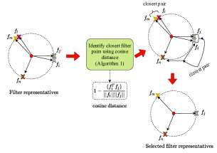
An illustration of similar convolutional filters where similarity is measured using cosine distance in filter representative space is shown in Figure 1. Such similar filters mostly contribute to redundancy in CNNs [16] and hence, can be eliminated. Eliminating redundancy in CNNs can reduce the number of parameters or memory storage and speed-up CNNs during their inference as well [17]. In addition, the carbon footprint generated during training of CNNs reduce as training time per epoch decreases in compressed CNNs [18]. A few of the important convolutional filters selected using Algorithm 1 proposed in Section 3 are also shown in Figure 1.

Figure 1: An illustration of a few important convolutional filters selected in a convolutional layer of CNN from a given set of filters using Algorithm 1. Here, each filter is represented in a filter representative space.

The rest of this paper is organised as follows. Section 2 gives a brief overview on filter pruning methods to remove CNN parameters. The proposed framework to identify similar filters is described in Section 3. Next, Section 4 includes experimental setup and Section 5 presents results and analysis. Finally, the discussion and conclusion is presented in Section 6 and Section 7 respectively.

2 Filter Pruning Methods

Filter pruning methods [19, 20] have been widely employed to eliminate convolutional filters based on their importance and to yield a pruned network. The importance can be measured either in an active manner that involves a dataset [16, 19, 21, 22, 23] or in a passive manner [20, 24] that does not involve a dataset. Mostly, active filter pruning methods measure entropy [25], variance [26] or similarity [16] in the outputs produced by each filter across dataset to quantify their importance. On the other hand, passive filter pruning methods [20, 27] rely only on convolution filters to quantify their importance without involving any dataset, and hence are relatively simpler than active filter pruning methods.

Majority of the existing passive filter pruning methods are norm-based that uses e.g. $l_{1}$-norm [20] of the filters to quantify their importance. A filter with relatively low norm is considered to be less important. After ranking filters based on their importance, few filters are eliminated based on a user-defined pruning ratio. Eliminating filters reduce performance of the pruned network, which is regained by performing a fine-tuning step.

The efficacy of passive norm-based filter pruning methods in defining importance of each filter depend on two conditions: (a) the minimum norm of the filter should be close to zero, and (b) the difference between the minimum and maximum norm of the filters should be as large as possible. However, such conditions are not always satisfied [28].

This paper proposes a passive filter pruning approach to compress any pre-trained convolutional neural networks designed for ASC. The proposed approach eliminates convolutional filters based on their similarity rather than considering filter norm, and does not require any user-defined pruning ratio. Our hypothesis is that few of the convolutional filters in CNNs are similar and such filters give mostly redundant information. Therefore, one of the similar filters can be eliminated from the network without much loss of performance. In the proposed approach, we consider the relationship among convolutional filters by measuring their cosine-similarity to quantify their importance and proposes an Algorithm 1 to select few important convolutional filters.

We also analyse how many training examples are sufficient in the fine-tuning process to achieve similar performance to that obtained using all training examples. The major contributions of this paper are summarised as follows:

• We propose a passive filter pruning framework which removes similar filters from a pre-trained CNN without any requirement of user-defined pruning ratio.

• We show that a pruned network obtained using the proposed pruning outperforms an existing $l_{1}$-norm based pruning method.

• We show that a reduction of training examples by 25% during fine-tuning process gives a similar performance with reduced training time.

3 Proposed Method

Consider a convolutional layer in a CNN which has $n$ filters denoted by $F_{i}$, $1\leq i\leq n$. Each filter has the same size with width $w$, height $h$ and number of channels $c$. Given the $n$ filters from the convolutional layer, our aim is to identify similar filters and select few important filters.

First, each filter is transformed into a 2-D matrix of size ($wh\times c$), where each column is obtained by stacking the width and height parameters. Next, we find Rank-1 approximation of each filter by performing singular value decomposition (SVD) that gives best Rank-1 approximation with respect to the Frobenius norm.

A filter $F_{i}$ is approximated as $\hat{F}_{i}$ = $\sigma_{1}u_{1}v^{T}_{1}$, where $\sigma_{1}$ denotes the significant singular value, $u_{1}$ denotes first left singular vector and $v_{1}$ denotes first right singular vector. Next, $\hat{F}_{i}$ is normalised column-wise and any column from the normalised $\hat{F}_{i}$ is chosen that acts as a “filter representative”, $f_{i}$. It is important to note that each column in the normalised $\hat{F}_{i}$ is same as $\hat{F}_{i}$ has unit rank. After obtaining filter representatives corresponding to each filter, we compute the pairwise cosine distance between filter representatives. This gives a similarity matrix, $\mathbf{W}\in\mathbb{R}^{n\times n}$. Now, given the similarity matrix, a greedy Algorithm 1 is proposed to identify important filters.

To identify important filters, we select the closest pair for each filter representative using $\mathbf{W}$, and sorted each closest pair according to their distance in the order of low to high. Here, the cosine distance between the closest pair defines their importance.

Next, we define one of the filter representative as important or redundant from each closest pair starting from the least important closest filter pair. A filter representative (the first index) from the least important closest pair is chosen as an important and other as a redundant. This procedure is repeated for each closest pair in the order of their importance except for the closest filter pair containing already identified redundant filter representative. Finally, a set of important filter representatives are obtained after ignoring all redundant filter representatives. An illustration of the important filters selected using Algorithm 1 is shown in Figure 1.

The redundant filters obtained using Algorithm 1 are explicitly eliminated form the unpruned network to yield a pruned network. The pruned network thus obtained has reduced number of parameters, less computational complexity and loss in performance due to elimination of few filters. To regain lost performance, a fine-tuning step is performed which involves a training dataset to re-train the pruned network. The proposed pruning algorithm can be found at: https://gitlab.surrey.ac.uk/as0150/passive-pruning.

Data: Pair-wise cosine distance of $n$ filters

($\mathbf{W}$ $\in\mathbb{R}^{n\times n}$).

Result: Indices of important filters (Imp_list)

A= [ ], Imp_list =[ ], Red_list = [ ]

for $i\leq n$ do

        [$m$, $d$] = argmin{ $\mathbf{W}$[ i, : - {i}] } ;

         /* Identify the closet filter $m$ to $i^{th}$ filter with their distance $d$. */

        A.append($(i,m)$, $d$);

end for

A_sort = Sort(A) ;

  /* Sort $A$ based on the distance $d$. */

for $i\leq len(\text{{A}})$ do

        index_imp = A_sort[i][0];

         /* important filter index */

        index_red= A_sort[i][1] ;

         /* redundant filter index */

        if index_imp $\notin$ Red_list then

              Imp_list.append( index_imp );

               Red_list.append( index_red )

        end if

       

end for

Algorithm 1 Identification of important filters

4 Experimental Setup

We evaluate the proposed method on the publicly available DCASE 2021 Task1A baseline [10] network to this we refer as the unpruned network that accepts log-mel energies of size $40\times 500$ extracted from 10-second audio signals as input. The unpruned network has three convolutional layers (C1, C2, C3) with 16, 16 and 32 number of filters respectively. These are followed by a dense layer of 100 units and a classification layer of 10 units.

The unpruned network is trained on TAU Urban Acoustic Scenes 2020 Mobile [9] development training dataset to classify 10 acoustic scenes recorded using multiple devices for 200 epochs using Adam optimizer with learning rate 0.001. The unpruned network gives 48.58% accuracy on validation dataset, has 46246 parameters and requires 286M multiply-accumulate operations (MACs) per inference to produce an output corresponding to 10-second audio signal. For fine-tuning the pruned network, we opt similar conditions as used in training the unrpuned network except 30 fine-tuning epochs, which are reduced by approximately 7x than that used in training the unpruned network.

The effectiveness of the proposed pruning method is measured in terms of accuracy obtained with or without fine-tuning, reduced MACs per inference and reduced number of parameters in the pruned network. To report performance after fine-tuning, we fine-tune the pruned network independently for 5 times and reported average accuracy.

The proposed pruning method is compared to an $l_{1}$-norm based pruning method [20]. The $l_{1}$-norm based method ranks convolutional filters according to their norm and requires user-defined pruning ratio. Therefore, we choose the same pruning ratio for $l_{1}$-norm method as obtained using our proposed method. The experiments are performed on GeForce RTX 2070 with Max-Q Design computing device.

5 Results & Analysis

The number of redundant filters obtained using the proposed pruning method in C1, C2 and C3 layers are 5, 5 and 10 respectively. The cosine distance of filters in C3 layer have relatively smaller deviation than that of other layers as shown in Figure 2. Due to this, the number of redundant filters in the C3 layer are more than that of other layers.

Figure 2: Histogram of distance between closest filter pairs across different convolutional layers. The mean $\mu$ and standard deviation $\sigma$ of cosine distance is also given.

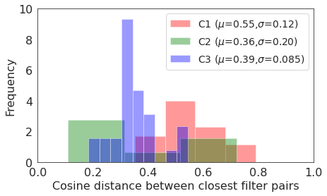
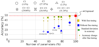
Figure 3 shows the performance obtained after pruning different subset of layers. Without performing any fine-tuning, the accuracy in the pruned network degrades. Pruning C3 layer gives maximum reduction in accuracy in comparison to that of C1 and C2 layers. Also, pruning other layers in combination C3 layer shows relatively more degradation. We speculate that this is due to the significant alteration of decision boundaries learned by dense and classification layer as C3 is a bottleneck layer.

After performing fine-tuning, the accuracy of the pruned networks improve significantly as shown in Figure 3. The accuracy obtained after fine-tuning C1 layer is similar to that of the unpruned network at 9% reduction in parameters and 1.8% reduction in MACs. Even though C3 layer has more redundant filters yet C3 layer reduces only 2.2% MACs with 22% reduced parameters and 1% drop in accuracy. On the other hand, pruning C2 layer reduces 27% MACs with 25% reduction in parameters at less than 1% drop in accuracy.

In contrast to pruning individual layers, pruning two or more layers reduce more MACs and parameters at relatively larger drop in accuracy. As an instance, pruning (C1+C2+C3) layers reduce approximately 31% MACs and 48% parameters at less than 4% drop in accuracy.

Figure 3: Various parameters obtained by pruning different layers in DCASE 2021 Task1A baseline network. Here, CX (“M”) means that the MACs have reduced by M% after pruning X^th convolutional layer. The accuracy is obtained with or without fine-tuning. The standard deviation in accuracy is obtained after fine-tuning the pruned network independently for 5 times using 100% training dataset.

Comparison with $l_{1}$-norm based pruning: The $l_{1}$-norm of the filters in C2 layer is shown in Figure 4. It can be observed that the top-5 filters with relatively low norm may be still significant as the ratio of the lowest norm to highest norm is greater than 84%. This verifies that the norm of the filter alone may not be a good metric to define filter importance.

Figure 4: $l_{1}$-norm of the filters in C2 layer and top 11 filters selected using the proposed method. $l_{1}$-norm method ignores relatively low-norm filters indexed {13, 4, 5, 1, 7}.

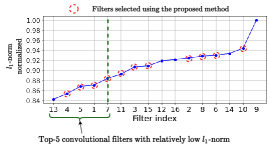
On the other hand, our proposed method does not use norm of the filters and rely on similarity among filters to select filters. It can be seen in Figure 4 that our method selects filters with indices {4,5,1,7} which are ignored by $l_{1}$-norm method.

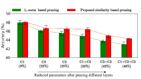
Choosing filters based on similarity improves performance of the pruned network as compared to norm-based method. It can be observed from Figure 5 that the accuracy obtained using the proposed similarity-based pruning is better than that of norm-based pruning across various layers. In particular, the proposed method improves accuracy by (1-1.5)%, when the number of reduced parameters are more.

Figure 5: Accuracy obtained using proposed method and $l_{1}$-norm method after fine-tuning the pruned network using 100% training dataset when different layers are pruned.

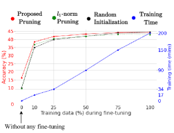
Analysis of fine-tuning at different training examples: Next, we analyse the computational complexity during fine-tuning and the accuracy obtained after fine-tuning the pruned network by varying training examples from 10% to 100% that is shown in Figure 6. The pruned network is obtained by pruning (C1+C2+C3) layers using the proposed method or $l_{1}$-norm method. Also, we fine-tune a pruned network where the parameters of the pruned network are initialized randomly.

Without performing any fine-tuning, the accuracy of the pruned network obtained using the proposed pruning method is approximately 6 percentage points better than that of $l_{1}$-norm method or randomly initialized network. Also, the proposed pruning framework gives similar or better performance than $l_{1}$-norm method and randomly initialized network after performing fine-tuning. It is also interesting to note that the randomly initialized network performs similar to the pruned network obtained using the proposed pruning method when more training dataset ($\geq$ 75%) is used in fine-tuning.

The pruned network significantly improves performance from 16% to 40% at 12x reduction in training time when fine-tuned with only 10% training dataset in contrast to that of using all training dataset. Utilizing 75% training dataset in fine-tuning the pruned network gives similar performance as that of all training dataset with 1.33x (25%) reduction in training time.

Figure 6: Accuracy and training time required to fine-tune by 30 epochs after pruning (C1 + C2 + C3) layers, when the number of training examples are varied from 10% to 100%.

6 Discussion

The proposed pruning method produces a low-complexity pruned network that achieves similar performance as that of the unpruned network after performing fine-tuning for only 30 epochs.

Pruning filters using the proposed method gives a set of important filters with improved performance in contrast to that of $l_{1}$-norm method. The proposed method is particularly advantageous when more parameters are eliminated. Moreover, the proposed method automatically selects number of important filters and does not require any user-defined pruning ratio.

Table 1: Accuracy of the pruned network obtained after pruning (C1+C2+C3) layers without performing any fine-tuning when different methods are used to select important filters.

Method to obtain Pruned network (C1+C2+C3)	Accuracy
Proposed cosine distance based method	16.23%
Chebyshev distance based method	12.23%
Average filters	10%
$l_{1}$-norm method	9.84%
Randomly initialized pruned network	10%

We compare other methods such as Chebyshev distance and average filters to compute important set of filters in the pruned network (C1+C2+C3) for analysing the effectiveness of the proposed pruning method. In Chebyshev distance method, we use the Chebyshev distance which is defined as the maximum of differences along any filter representative dimension to generate similarity matrix in Algorithm 1. In average filters method, we compute closest filter pairs based on cosine distance, and generate new filters by averaging the closest filter pairs.

The accuracy of the pruned network without performing any fine-tuning using the proposed method outperforms the other methods as given in Table 1. The performance obtained after averaging the similar filters is more or less random. In contrast to Chebyshev distance, the cosine distance shows promising result.

7 Conclusions and Future work

We propose a cosine distance based passive filter pruning framework to compress a pre-trained convolutional neural network. The proposed framework identifies pruning ratio automatically. We find that considering pair-wise relationships among filters yield a better set of important filters and improves performance compared to norm-based filters selection. We also observe that fine-tuning the pruned network for few epochs and using few training examples improves the performance of the pruned network significantly. Our future goal is to design better distance metrics to measure pair-wise similarity among filters and to reduce the performance loss in the pruned network with minimal requirement of fine-tuning.

8 Acknowledgements

This work was supported by Engineering and Physical Sciences Research Council (EPSRC) Grant EP/T019751/1 “AI for Sound”.

References

- [1] D. Barchiesi, D. Giannoulis, D. Stowell, and M. D. Plumbley, “Acoustic scene classification: Classifying environments from the sounds they produce,” IEEE Signal Processing Magazine, vol. 32, no. 3, pp. 16–34, 2015.
- [2] Y. Xu, W. J. Li, and K. K. Lee, Intelligent Wearable Interfaces. John Wiley & Sons, 2008.
- [3] P. Temdee and R. Prasad, Context-aware Communication and Computing: Applications for smart environment. Springer, 2018.
- [4] Z. Yang, M. Chen, K.-K. Wong, H. V. Poor, and S. Cui, “Federated Learning for 6G: Applications, challenges, and opportunities,” Engineering, vol. 8, pp. 33–41, 2022.
- [5] D. Stowell, D. Giannoulis, E. Benetos, M. Lagrange, and M. D. Plumbley, “Detection and classification of acoustic scenes and events,” IEEE Transactions on Multimedia, vol. 17, no. 10, pp. 1733–1746, Oct 2015.
- [6] A. Mesaros, T. Heittola, and T. Virtanen, “A multi-device dataset for urban acoustic scene classification,” Proceedings of the Detection and Classification of Acoustic Scenes and Events Workshop (DCASE2018), pp. 9–13, November 2018.
- [7] A. Mesaros, T. Heittola, E. Benetos, P. Foster, M. Lagrange, T. Virtanen, and M. D. Plumbley, “Detection and classification of acoustic scenes and events: Outcome of the DCASE 2016 challenge,” IEEE/ACM Transactions on Audio, Speech, and Language Processing, vol. 26, no. 2, pp. 379–393, Feb 2018.
- [8] A. Mesaros, A. Diment, B. Elizalde, T. Heittola, E. Vincent, B. Raj, and T. Virtanen, “Sound event detection in the DCASE 2017 challenge,” IEEE/ACM Transactions on Audio, Speech, and Language Processing, vol. 27, no. 6, pp. 992–1006, 2019.
- [9] T. Heittola, A. Mesaros, and T. Virtanen, “Acoustic scene classification in DCASE 2020 Challenge: generalization across devices and low complexity solutions,” proceedings of the Detection and Classification of Acoustic Scenes and Events (DCASE) Workshop, pp. 56–60, 2020.
- [10] I. Martín-Morató, T. Heittola, A. Mesaros, and T. Virtanen, “Low-complexity acoustic scene classification for multi-device audio: Analysis of DCASE 2021 challenge systems,” Detection and classification of acoustic scenes and events (DCASE) Workshop, pp. 85–89, 2021.
- [11] J. Abeßer, “A review of deep learning based Methods for acoustic scene classification,” Applied Sciences, vol. 10, no. 6, pp. 1–16, 2020.
- [12] Q. Kong, Y. Cao, T. Iqbal, Y. Wang, W. Wang, and M. D. Plumbley, “PANNs: Large-scale pretrained audio neural networks for audio pattern recognition,” IEEE/ACM Transactions on Audio, Speech, and Language Processing, vol. 28, pp. 2880–2894, 2020.
- [13] Q. Wang, W. Huang, Z. Xiong, and X. Li, “Looking closer at the scene: Multiscale representation learning for remote sensing image scene classification ,” IEEE Transactions on Neural Networks and Learning Systems (in press), pp. 1–15, 2020.
- [14] E. L. Denton, W. Zaremba, J. Bruna, Y. LeCun, and R. Fergus, “Exploiting linear structure within convolutional networks for efficient evaluation,” Advances in Neural Information Processing systems, vol. 27, pp. 1269–1277, 2014.
- [15] K. Kahatapitiya and R. Rodrigo, “Exploiting the redundancy in convolutional filters for parameter reduction,” proceedings of the IEEE/CVF Winter Conference on Applications of Computer Vision, pp. 1410–1420, 2021.
- [16] A. Singh, P. Rajan, and A. Bhavsar, “Deep hidden analysis: A statistical framework to prune feature maps,” IEEE International Conference on Acoustics, Speech and Signal Processing (ICASSP), pp. 820–824, 2019.
- [17] Y.-D. Kim, E. Park, S. Yoo, T. Choi, L. Yang, and D. Shin, “Compression of deep convolutional neural networks for fast and low power mobile applications,” International Conference on Learning Representations, ICLR (arXiv preprint arXiv:1511.06530), 2016.
- [18] A. Lacoste, A. Luccioni, V. Schmidt, and T. Dandres, “Quantifying the carbon emissions of machine learning,” arXiv preprint arXiv:1910.09700, 2019.
- [19] P. Molchanov, S. Tyree, T. Karras, T. Aila, and J. Kautz, “Pruning convolutional neural networks for resource efficient inference,” International Conference on Learning Representations, ICLR, 2017.
- [20] H. Li, A. Kadav, I. Durdanovic, H. Samet, and H. P. Graf, “Pruning filters for efficient convnets,” International Conference on Learning Representations, ICLR, 2017.
- [21] J.-H. Luo, J. Wu, and W. Lin, “ThiNet: A filter level pruning method for deep neural network compression,” proceedings of the IEEE International Conference on Computer Vision, pp. 5058–5066, 2017.
- [22] H. Hu, R. Peng, Y.-W. Tai, and C.-K. Tang, “Network Trimming: A data-driven neuron pruning approach towards efficient deep architectures ,” arXiv preprint arXiv:1607.03250, 2016.
- [23] S. Lin, R. Ji, C. Yan, B. Zhang, L. Cao, Q. Ye, F. Huang, and D. Doermann, “Towards optimal structured CNN pruning via generative adversarial learning,” Proceedings of the IEEE/CVF Conference on Computer Vision and Pattern Recognition, pp. 2790–2799, 2019.
- [24] H. Zhuo, X. Qian, Y. Fu, H. Yang, and X. Xue, “SCSP: Spectral clustering filter pruning with soft self-adaption manners,” arXiv preprint arXiv:1806.05320, 2018.
- [25] Y. Li, L. Wang, S. Peng, A. Kumar, and B. Yin, “Using feature entropy to guide filter pruning for efficient convolutional networks,” International Conference on Artificial Neural Networks, pp. 263–274, 2019.
- [26] A. Polyak and L. Wolf, “Channel-level acceleration of deep face representations,” IEEE Access, vol. 3, pp. 2163–2175, 2015.
- [27] Y. He, P. Liu, Z. Wang, Z. Hu, and Y. Yang, “Filter pruning via geometric median for deep convolutional neural networks acceleration,” proceedings of the IEEE/CVF Conference on Computer Vision and Pattern Recognition, pp. 4340–4349, 2019.
- [28] M. Park, W. Kim, and S. Kim, “REPrune: Filter pruning via representative election,” arXiv preprint arXiv:2007.06932, 2020.