Exact Community Recovery
in Correlated Stochastic Block Models

Abstract

We consider the problem of learning latent community structure from multiple correlated networks. We study edge-correlated stochastic block models with two balanced communities, focusing on the regime where the average degree is logarithmic in the number of vertices. Our main result derives the precise information-theoretic threshold for exact community recovery using multiple correlated graphs. This threshold captures the interplay between the community recovery and graph matching tasks. In particular, we uncover and characterize a region of the parameter space where exact community recovery is possible using multiple correlated graphs, even though (1) this is information-theoretically impossible using a single graph and (2) exact graph matching is also information-theoretically impossible. In this regime, we develop a novel algorithm that carefully synthesizes algorithms from the community recovery and graph matching literatures.

1 Introduction

Recovering communities in networks is a fundamental learning task that has myriad applications in sociology, biology, and beyond. Increasingly, network data is supplemented with further data that is correlated with the underlying communities, such as latent feature vectors (e.g., the interests of individuals in a social network) or further correlated networks (e.g., personal and professional social networks overlap, yet contain complementary information). Synthesizing information from these different data sources presents an opportunity to obtain improved community recovery algorithms and guarantees, yet this comes with algorithmic and statistical challenges. In particular, integrating information from correlated networks is often hindered because the graphs are not aligned, due to node labels that are missing, erroneous, anonymized, or otherwise unknown. This highlights the importance of graph matching, which is an important learning task in its own right.

Recently, Rácz and Sridhar [RS21] determined the information-theoretic limits for exact graph matching in edge-correlated stochastic block models, and as an application they showed how to exactly recover communities from two correlated graphs in a regime where it is impossible to do so using just a single graph. The main contribution of our work is to go beyond exact graph matching, and we determine the precise information-theoretic threshold for exact community recovery from two correlated block models. In particular, we uncover and characterize a region of the parameter space where exact community recovery is possible despite exact graph matching being impossible (and exact community recovery from a single graph also being impossible), positively resolving a conjecture of [RS21]. To do so, we develop a novel algorithm that carefully synthesizes community recovery and graph matching algorithms. Overall, our work highlights the subtle interplay between community recovery and graph matching, two canonical and widely-studied learning problems.

1.1 Community recovery in correlated stochastic block models

The stochastic block model (SBM). The SBM is the canonical probabilistic generative model for networks with community structure. Introduced by Holland, Laskey, and Leinhardt [HLL83], it has received enormous attention over the past decades; in particular, it serves as a natural theoretical testbed for evaluating and comparing clustering algorithms on average-case networks (see, e.g., [dyer1989solution, bui1984graph, bopanna1987eigenvalues]). The SBM allows a precise understanding of when community information can be extracted from network data, due to the fact that it exhibits sharp information-theoretic phase transitions for various inference tasks. Such phase transitions were first conjectured by Decelle et al. [DKMZ11] and were subsequently proven rigorously by several authors [mossel2014reconstruction, massoulie2014community, mossel2018proof, abbe2016exact, mossel2016consistency, abbe2015community, bordenave2015nonbacktracking, Abbe_survey].

Here we focus on the SBM with two symmetric communities, arguably the simplest setting. For a positive integer $n$ and $p,q\in[0,1]$, we construct the graph $G\sim\mathrm{SBM}(n,p,q)$ as follows. The graph $G$ has $n$ vertices, labeled by the elements of $[n]:=\{1,\ldots,n\}$. Each vertex $i\in[n]$ has a community label $\sigma_{*}(i)\in\{+1,-1\}$; these are drawn i.i.d. uniformly at random across all $i\in[n]$. The vector of community labels is denoted by $\boldsymbol{\sigma_{*}}:=\{\sigma_{*}(i)\}_{i=1}^{n}$, with the two communities given by the sets $V^{+}:=\{i\in[n]:\sigma_{*}(i)=+1\}$ and $V^{-}:=\{i\in[n]:\sigma_{*}(i)=-1\}$. Given the community labels $\boldsymbol{\sigma_{*}}$, the edges of $G$ are drawn independently across vertex pairs as follows. For distinct $i,j\in[n]$, if $\sigma_{*}(i)\sigma_{*}(j)=1$ (i.e., $i$ and $j$ are in the same community), then the edge $(i,j)$ is in $G$ with probability $p$; else, $(i,j)$ is in $G$ with probability $q$.

Community recovery. In this setting, a community recovery algorithm takes as input the graph $G$, without knowledge of the community labels $\boldsymbol{\sigma_{*}}$, and outputs a community labeling $\widehat{\boldsymbol{\sigma}}$. The success of an algorithm is measured by the overlap between the estimated labeling and the ground truth, defined as

$$\mathsf{ov}(\widehat{\boldsymbol{\sigma}},\boldsymbol{\sigma_{*}}):=\frac{1}{n}\left|\sum\limits_{i=1}^{n}\widehat{\sigma}(i)\sigma_{*}(i)\right|.$$

We take an absolute value in this formula since the labelings $\boldsymbol{\sigma_{*}}$ and $-\boldsymbol{\sigma_{*}}$ specify the same partition of communities, and it is only possible to recover $\boldsymbol{\sigma_{*}}$ up to its sign. Observe that $\mathsf{ov}(\widehat{\boldsymbol{\sigma}},\boldsymbol{\sigma_{*}})\in[0,1]$, with a larger value corresponding to a better estimate. In particular, the algorithm succeeds in exactly recovering the communities (i.e., $\widehat{\boldsymbol{\sigma}}=\boldsymbol{\sigma_{*}}$ or $\widehat{\boldsymbol{\sigma}}=-\boldsymbol{\sigma_{*}}$) if and only if $\mathsf{ov}(\widehat{\boldsymbol{\sigma}},\boldsymbol{\sigma_{*}})=1$.

In the logarithmic degree regime—that is, when $p=\alpha\log(n)/n$ and $q=\beta\log(n)/n$ for some fixed constants $\alpha,\beta\geq 0$—it is well-known that there is a sharp information-theoretic threshold for exactly recovering communities in the SBM [abbe2016exact, mossel2016consistency, abbe2015community, Abbe_survey]. This is governed by the quantity

$$\mathrm{D_{+}}(\alpha,\beta):=\left(\frac{\sqrt{\alpha}-\sqrt{\beta}}{\sqrt{2}}\right)^{2}=\frac{\alpha+\beta}{2}-\sqrt{\alpha\beta}.$$ (1.1)

In the general setting, this quantity is known as the Chernoff-Hellinger divergence [abbe2015community, Abbe_survey]; in the specific setting of two balanced communities, it simplifies to the Hellinger divergence of the vectors $(\alpha/2,\beta/2)$ and $(\beta/2,\alpha/2)$, giving (1.1). The information-theoretic threshold for exact community recovery is then given by

$$\mathrm{D_{+}}(\alpha,\beta)=1.$$ (1.2)

If $\mathrm{D_{+}}(\alpha,\beta)>1$, then exact community recovery is possible: there is a polynomial-time algorithm which outputs an estimator $\widehat{\boldsymbol{\sigma}}$ satisfying $\lim_{n\to\infty}\mathbb{P}(\mathsf{ov}(\widehat{\boldsymbol{\sigma}},\boldsymbol{\sigma_{*}})=1)=1$. Moreover, if $\mathrm{D_{+}}(\alpha,\beta)<1$, then this is impossible: for any estimator $\widetilde{\boldsymbol{\sigma}}$, we have that $\lim_{n\to\infty}\mathbb{P}(\mathsf{ov}(\widetilde{\boldsymbol{\sigma}},\boldsymbol{\sigma_{*}})=1)=0$.

Correlated SBMs. The goal of our work is to understand how the exact community recovery threshold given by (1.2) changes when the input data consists of multiple correlated SBMs. To this end, we study a natural model of correlated SBMs, which we describe next.

We construct $(G_{1},G_{2})\sim\mathrm{CSBM}(n,p,q,s)$ as follows, where the additional parameter $s\in[0,1]$ controls the level of correlation between the two graphs. First, generate a parent graph $G\sim\mathrm{SBM}(n,p,q)$, and let $\boldsymbol{\sigma_{*}}$ denote the community labels. Next, given $G$, we construct $G_{1}$ by independent subsampling: each edge of $G$ is included in $G_{1}$ with probability $s$, independently of everything else, and non-edges of $G$ remain non-edges in $G_{1}$. We obtain a second graph, $G_{2}^{\prime}$, independently in the same way. The graphs $G_{1}$ and $G_{2}^{\prime}$ inherit both the vertex labels and the community labels $\boldsymbol{\sigma_{*}}$ from the parent graph $G$. Finally, we let $\pi_{*}$ be a uniformly random permutation of $[n]$, independently of everything else, and generate $G_{2}$ by relabeling the vertices of $G_{2}^{\prime}$ according to $\pi_{*}$ (e.g., vertex $i$ in $G_{2}^{\prime}$ is relabeled to $\pi_{*}(i)$ in $G_{2}$). This last step in the construction of $G_{2}$ reflects the fact that in applications, node labels are often obscured. To emphasize the effect of the vertex relabeling on the community labels, we define $\boldsymbol{\sigma_{*}^{1}}:=\boldsymbol{\sigma_{*}}$ and $\boldsymbol{\sigma_{*}^{2}}:=\boldsymbol{\sigma_{*}}\circ\pi_{*}^{-1}$, which are the community labels in $G_{1}$ and $G_{2}$, respectively. This construction is visualized in Figure 1.

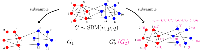
Figure 1: Schematic showing the construction of correlated SBMs (see text for details).

First studied by Onaran, Garg, and Erkip [onaran2016optimal], this model of correlated SBMs is the natural generalization of correlated Erdős-Rényi random graphs, which were introduced by Pedarsani and Grossglauser [pedarsani2011privacy] (see Section 1.4 for discussion of further related work). In particular, marginally $G_{1}$ and $G_{2}$ are both SBMs. Specifically, since the subsampling probability is $s$, we have that $G_{1}\sim\mathrm{SBM}(n,ps,qs)$. Therefore, from (1.2) it follows that, in the logarithmic degree regime where $p=\alpha\log(n)/n$ and $q=\beta\log(n)/n$, the communities can be exactly recovered from $G_{1}$ alone if $\mathrm{D_{+}}(\alpha s,\beta s)>1$. Since $\mathrm{D_{+}}(\alpha s,\beta s)=s\mathrm{D_{+}}(\alpha,\beta)$, this condition is equivalent to $s\mathrm{D_{+}}(\alpha,\beta)>1$, which we can also write as $\mathrm{D_{+}}(\alpha,\beta)>1/s$.

The central question of our work is how to go beyond this single-graph threshold by incorporating the information in $G_{2}$. This question was initiated in recent work of Rácz and Sridhar [RS21], whose starting observation was the following. If $\pi_{*}$ were known, then we can reconstruct $G_{2}^{\prime}$ from $G_{2}$, and then “overlay” $G_{1}$ and $G_{2}^{\prime}$ to obtain a new graph $H_{*}$ that combines the information in the two graphs. In particular, $(i,j)$ is an edge in $H_{*}$ if and only if $(i,j)$ is an edge in the parent graph $G$ and it is included in either $G_{1}$ or $G_{2}^{\prime}$ in the subsampling process. It thus follows that $H_{*}$ is also an SBM, specifically, $H_{*}\sim\mathrm{SBM}\left(n,\alpha(1-(1-s)^{2})\log(n)/n,\beta(1-(1-s)^{2})\log(n)/n\right)$. In particular, this argument implies that if $\pi_{*}$ were known and

$$\frac{1}{1-(1-s)^{2}}<\mathrm{D_{+}}(\alpha,\beta)<\frac{1}{s},$$

then it is information-theoretically impossible to exactly recover $\boldsymbol{\sigma_{*}}$ from $G_{1}$ alone, but one can recover $\boldsymbol{\sigma_{*}}$ exactly by combining information from $G_{1}$ and $G_{2}$.

Graph matching. Since $\pi_{*}$ is not known, the argument above raises the question of when can $\pi_{*}$ be exactly recovered from $(G_{1},G_{2})$, a task known as graph matching. The main result of Rácz and Sridhar [RS21] answers this question (see also Section 1.4 for discussion of related work). Specifically, they show that the information-theoretic threshold for exactly recovering $\pi_{*}$ is given by $s^{2}\left(\alpha+\beta\right)/2=1$. Note that this is precisely the connectivity threshold for the intersection graph of $G_{1}$ and $G_{2}^{\prime}$ (the edges of this intersection graph are the edges present in the parent graph $G$ that survived both subsampling processes). Letting

$$\mathrm{T_{c}}(\alpha,\beta):=\frac{\alpha+\beta}{2}$$ (1.3)

denote the connectivity threshold in $\mathrm{SBM}(n,\alpha\log(n)/n,\beta\log(n)/n)$, we can write the threshold for exactly recovering $\pi_{*}$ as $\mathrm{T_{c}}(\alpha s^{2},\beta s^{2})=1$, or equivalently, $s^{2}\mathrm{T_{c}}(\alpha,\beta)=1$. Thus, if $s^{2}\mathrm{T_{c}}(\alpha,\beta)>1$, then $\pi_{*}$ can be exactly recovered from $(G_{1},G_{2})$, while if $s^{2}\mathrm{T_{c}}(\alpha,\beta)<1$, then this is impossible.

To summarize the two previous paragraphs, Rácz and Sridhar [RS21] showed that if

$$s^{2}\mathrm{T_{c}}(\alpha,\beta)>1\qquad\qquad\text{ and }\qquad\qquad\left(1-(1-s)^{2}\right)\mathrm{D_{+}}(\alpha,\beta)>1,$$ (1.4)

then exact community recovery is possible, that is, it is possible to exactly recover $\boldsymbol{\sigma_{*}}$ using $(G_{1},G_{2})$.

The interplay between community recovery and graph matching. The work of Rácz and Sridhar [RS21] leaves open the question of what happens when exact graph matching is impossible. In particular, is there a parameter regime where exact community recovery is possible from $(G_{1},G_{2})$, even though (1) this is information-theoretically impossible using a single graph and (2) exact graph matching is also impossible?

We answer this question affirmatively, developing an algorithm that carefully combines community recovery and graph matching steps. Moreover, we determine the precise information-theoretic threshold for when exact community recovery is possible. If $\left(1-(1-s)^{2}\right)\mathrm{D_{+}}(\alpha,\beta)>1$, then this threshold is given by

$$\mathrm{T_{c}}\left(\alpha s^{2},\beta s^{2}\right)+\mathrm{D_{+}}\left(\alpha s(1-s),\beta s(1-s)\right)=1.$$ (1.5)

The threshold in (1.5) cleanly showcases the interplay between community recovery and graph matching: the first term in (1.5) comes from graph matching, while the second term comes from community recovery. We now turn to describing our results formally.

1.2 Results

We determine the information-theoretic threshold for exact community recovery from two correlated stochastic block models $(G_{1},G_{2})\sim\mathrm{CSBM}(n,\alpha\log(n)/n,\beta\log(n)/n,s)$. This result has two parts and we start with the positive one.

Theorem 1.1.

Fix constants $\alpha,\beta>0$ and $s\in[0,1]$. Let $(G_{1},G_{2})\sim\mathrm{CSBM}\left(n,\frac{\alpha\log n}{n},\frac{\beta\log n}{n},s\right)$. Suppose that

$$\left(1-(1-s)^{2}\right)\mathrm{D_{+}}(\alpha,\beta)>1$$ (1.6)

and that

$$s^{2}\mathrm{T_{c}}(\alpha,\beta)+s(1-s)\mathrm{D_{+}}(\alpha,\beta)>1.$$ (1.7)

Then there is an estimator $\widehat{\boldsymbol{\sigma}}=\widehat{\boldsymbol{\sigma}}(G_{1},G_{2})$ such that $\lim\limits_{n\to\infty}\mathbb{P}\left(\mathsf{ov}\left(\widehat{\boldsymbol{\sigma}},\boldsymbol{\sigma_{*}}\right)=1\right)=1.$

In the prior work [RS21] it was shown that (1.6) is necessary for exact community recovery, and that the conditions in (1.4) suffice. As described in Section 1.1, [RS21] focused on determining the exact graph matching threshold and then using community recovery algorithms as a black box. The main contribution of Theorem 1.1 is to go beyond exact graph matching, to showcase how exact community recovery is possible from $(G_{1},G_{2})$ even in regimes where (1) this is impossible from $G_{1}$ alone and (2) exact graph matching is impossible. This necessitates developing algorithms that combine information from $G_{1}$ and $G_{2}$ in more delicate ways, integrating ideas from community recovery and graph matching algorithms. Indeed, at a high level, the algorithm we develop to prove Theorem 1.1 has four main steps:

1. Obtain a partial almost exact graph matching $\widehat{\mu}$ between $G_{1}$ and $G_{2}$;

2. Obtain an almost exact community labeling of vertices in $G_{1}$;

3. For vertices in $G_{1}$ that are part of the matching $\widehat{\mu}$: refine the almost exact labeling obtained in Step (2) via a majority vote in the (denser) graph consisting of edges that are either in $G_{1}$ or in $G_{2}$ (determined using $\widehat{\mu}$).

4. For vertices in $G_{1}$ that are not part of the matching $\widehat{\mu}$: classify them according to a majority vote of the labels of their neighbors, where we use only the edges in $G_{1}$.

In order to make such an algorithm work, the devil is in the details, with careful choices in each step; we refer to Section 1.3 for a more detailed overview of the algorithm.

The threshold in (1.7) highlights the interplay between the community recovery and graph matching tasks. Indeed, the first term in (1.7) comes from graph matching: $s^{2}\mathrm{T_{c}}(\alpha,\beta)=1$ is the threshold for exact graph matching; moreover, when $s^{2}\mathrm{T_{c}}(\alpha,\beta)<1$, the best possible almost exact graph matching makes $n^{1-s^{2}\mathrm{T_{c}}(\alpha,\beta)+o(1)}$ errors, which is relevant for Step (1) of the algorithm. On the other hand, the second term in (1.7) comes from community recovery; in particular, this term arises from the majority vote in Step (4). Note that while we use all edges in $G_{1}$ for this step, the unmatched nodes are isolated in the intersection graph, and hence the relevant edges are not present in $G_{2}$, leading to the “effective” factor of $s(1-s)$. Since exact community recovery in $\mathrm{SBM}(n,\alpha s(1-s)\log(n)/n,\beta s(1-s)\log(n)/n)$ is governed by the quantity $\mathrm{D_{+}}(\alpha s(1-s),\beta s(1-s))=s(1-s)\mathrm{D_{+}}(\alpha,\beta)$, this leads to the second term in (1.7).

As the following impossibility result shows, Theorem 1.1 is tight.

Theorem 1.2.

Fix constants $\alpha,\beta>0$ and $s\in[0,1]$. Let $(G_{1},G_{2})\sim\mathrm{CSBM}\left(n,\frac{\alpha\log n}{n},\frac{\beta\log n}{n},s\right)$. Suppose that

$$\left(1-(1-s)^{2}\right)\mathrm{D_{+}}(\alpha,\beta)<1$$ (1.8)

or that

$$s^{2}\mathrm{T_{c}}(\alpha,\beta)+s(1-s)\mathrm{D_{+}}(\alpha,\beta)<1.$$ (1.9)

Then for any estimator $\widetilde{\boldsymbol{\sigma}}=\widetilde{\boldsymbol{\sigma}}(G_{1},G_{2})$, we have that $\lim\limits_{n\to\infty}\mathbb{P}(\mathsf{ov}(\widetilde{\boldsymbol{\sigma}},\boldsymbol{\sigma_{*}})=1)=0.$

Impossibility of exact community recovery under the condition (1.8) was shown in [RS21], so the contribution of Theorem 1.2 is to show impossibility under the condition (1.9).

As discussed above, the condition (1.9) highlights the interplay between the community recovery and graph matching tasks. In particular, Theorem 1.2 uncovers and characterizes a region of the parameter space where exact community recovery from $(G_{1},G_{2})$ is impossible, despite the fact that if $\pi_{*}$ were known, then exact community recovery would be possible from the correctly matched union graph $G_{1}\vee_{\pi_{*}}G_{2}$.

Putting together Theorems 1.1 and 1.2, we obtain the information-theoretic threshold for exact community recovery in correlated SBMs, see (1.5). These results are illustrated in the phase diagrams of Figures 2 and 3.

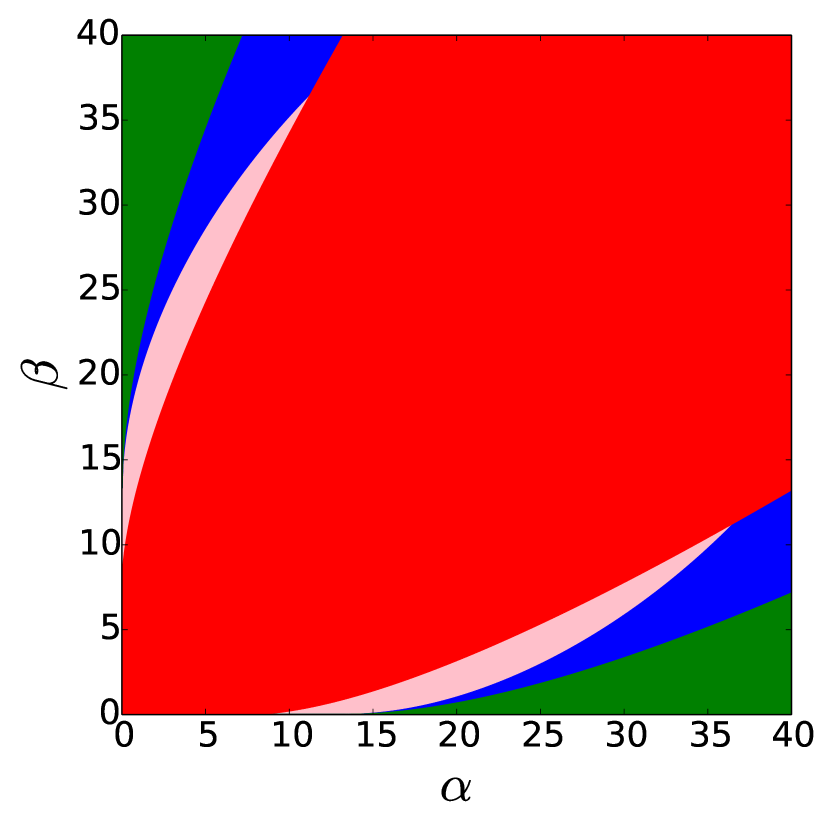
(a) Fixed $s=0.15$.

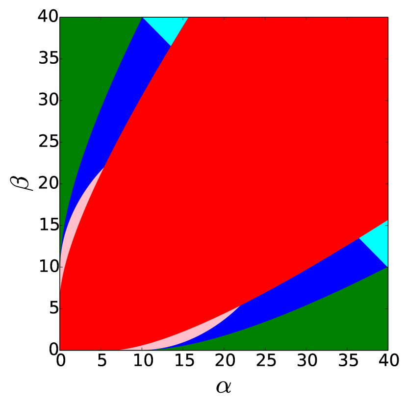
(b) Fixed $s=0.2$.

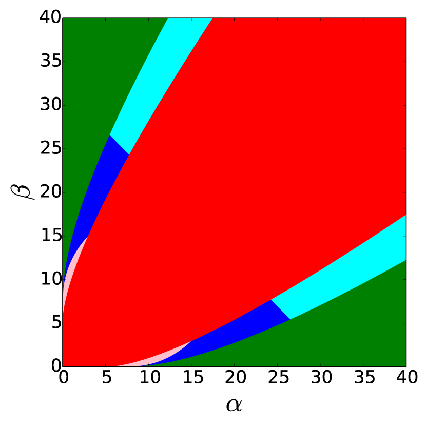
(c) Fixed $s=0.25$.

Figure 2: Phase diagram for exact community recovery for fixed $s$, with $\alpha\in[0,40]$ and $\beta\in[0,40]$ on the axes. Green region: exact community recovery is possible from $G_{1}$ alone; Cyan region: exact community recovery is impossible from $G_{1}$ alone, but exact graph matching is possible, and subsequently exact community recovery is possible from $(G_{1},G_{2})$; Dark Blue region: exact community recovery is impossible from $G_{1}$ alone, exact graph matching is also impossible, yet exact community recovery is nonetheless possible from $(G_{1},G_{2})$; Pink region: exact community recovery is impossible from $(G_{1},G_{2})$ (even though it would be possible if $\pi_{*}$ were known). Red region: exact community recovery is impossible from $(G_{1},G_{2})$ (even if $\pi_{*}$ is known). Characterizing the Dark Blue and Pink regions is the main result of this paper.

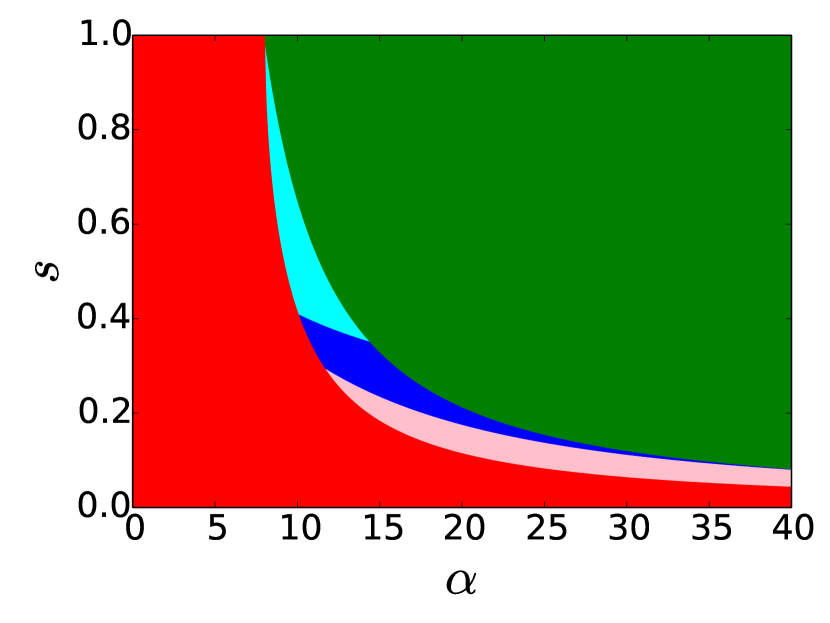
(a) Fixed $\beta=2$.

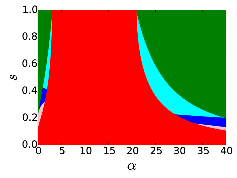
(b) Fixed $\beta=10$.

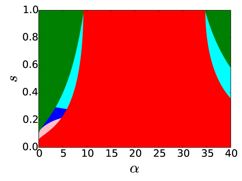
(c) Fixed $\beta=20$.

Figure 3: Phase diagrams for exact community recovery for fixed $\beta$, with $\alpha\in[0,40]$ and $s\in[0,1]$ on the axes. (Colors as in Fig. 2.)

1.3 Overview of algorithms and proofs

We next expand upon the very high-level steps of the recovery algorithm presented in Section 1.2, detailing choices made in each step, and highlighting technical challenges that arise in the analysis. We also give an overview of the impossibility proof.

Almost exact graph matching via the $k$-core estimator.

For a permutation $\pi:[n]\to[n]$, let $G_{1}\land_{\pi}G_{2}$ be the corresponding intersection graph of $G_{1}$ and $G_{2}$, where $(i,j)$ is an edge in $G_{1}\land_{\pi}G_{2}$ if and only if $(i,j)$ is an edge in $G_{1}$ and $(\pi(i),\pi(j))$ is an edge in $G_{2}$. The graph matching algorithm we study—called the $k$-core estimator—iterates over all permutations of $[n]$ and finds a permutation $\widehat{\pi}$ that induces the largest $k$-core in the corresponding intersection graph. The output of the algorithm is a potentially incomplete vertex correspondence $\widehat{\mu}$, which is the restriction of $\widehat{\pi}$ to the vertex set of the $k$-core in $G_{1}\land_{\widehat{\pi}}G_{2}$. Figure 4 provides an illustration.

While it is (information-theoretically) impossible that $\widehat{\mu}=\pi_{*}$ with probability larger than $o(1)$ in the parameter regime that we consider, $\widehat{\mu}$ has two important properties that we highlight. First, $\widehat{\mu}$ matches almost all vertices; that is, if we denote by $F$ the set of unmatched vertices, then $|F|=o(n)$. Second, the vertices matched by $\widehat{\mu}$ are all correct with probability $1-o(1)$. This property is extremely important for downstream community recovery tasks, as it allows us to clearly leverage information from $G_{1}$ and $G_{2}$ in classifying a given vertex in the correspondence $\widehat{\mu}$.

Intuitively, graph matching algorithms tend to fail in aligning vertices that are not well-connected in $G_{1}\land_{\pi_{*}}G_{2}$ (in particular, singletons), since such vertices have little common information across $G_{1}$ and $G_{2}$. On the other hand, the $k$-core is, by definition, a well-connected subgraph, explaining why the $k$-core estimator succeeds for an appropriate choice of $k$ (we choose $k=13$ in this paper). Previously, Cullina, Kiyavash, Mittal, and Poor [cullina2020partial] proved the almost exact correctness of the $k$-core estimator for sparse correlated Erdős-Rényi graphs. Here, we extend their results to correlated SBMs, which requires a novel analysis, since the prior work of [cullina2020partial] utilized certain probability generating functions that can only be tractably computed for Erdős-Rényi graphs. Our approach circumvents this issue while also providing a tight analysis for the logarithmic degree regime.

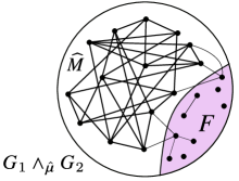
Figure 4: Illustration of the $k$-core matching (here, $k=4$). Pictured here is the corresponding $k$-core of the intersection graph $G_{1}\land_{\widehat{\mu}}G_{2}$.

An important and novel consequence of our analysis is that for correlated SBMs in the logarithmic degree regime, the $k$-core estimator achieves optimal performance. Specifically, we show that the $k$-core estimator fails to match at most $|F|\leq n^{1-s^{2}\mathrm{T_{c}}(\alpha,\beta)+o(1)}$ vertex pairs, which is orderwise equal to the number of singletons of $G_{1}\land_{\pi_{*}}G_{2}$, for which it is known that any graph matching algorithm will fail [RS21, cullina2016simultaneous]. This optimality of the $k$-core estimator is a fundamental reason why we utilize the $k$-core estimator to prove that the information-theoretic threshold can be achieved.

Exact community recovery in the correctly matched region.

Since exact community recovery is impossible in $G_{1}$ or in $G_{2}$ alone, we will utilize the almost-exact vertex alignment $\widehat{\mu}$ to combine information from both graphs to recover communities. The algorithm we design does so by recovering communities through multiple subroutines, each of which is executed carefully in order to de-couple the complex dependencies between $G_{1}$, $G_{2}$, and $\widehat{\mu}$. Initially, we focus on recovering the community labels of vertices that are part of the (partial) matching $\widehat{\mu}$.

First, we run a community recovery algorithm on $G_{1}$ to generate an almost-exact community labeling (i.e., with $o(n)$ errors). Using $\widehat{\mu}$, we then identify the graph $G_{1}\lor_{\widehat{\mu}}G_{2}$, which consists of edges $(i,j)$ such that $(i,j)$ is an edge in $G_{1}$ or $(\widehat{\mu}(i),\widehat{\mu}(j))$ is an edge in $G_{2}$. Using $G_{1}\lor_{\widehat{\mu}}G_{2}$, we then refine the almost-exact community labeling by re-classifying vertices in $\widehat{\mu}$ according to a majority vote among the labels of neighbors in $G_{1}\lor_{\widehat{\mu}}G_{2}$. See Figure 5 for an illustration.

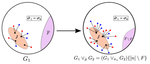
Figure 5: Illustration of how the recovery algorithm classifies vertices in $[n]\setminus\overline{F}$ (see Algorithm LABEL:alg:labeling-k-core). In each graph, the orange region denotes the set of incorrectly classified vertices resulting from applying Algorithm LABEL:alg:MNS (almost exact community recovery) to $G_{1}$, the purple region denotes $\overline{F}$ or $\overline{F}\setminus F$ (which are classified later), and the white region denotes the set of correctly-classified vertices. When the two graphs are overlayed to form $G_{1}\lor_{\widehat{\mu}}G_{2}$, all vertices in $J$ have a neighborhood majority corresponding to the correct community labeling.

To make this algorithm work, there are several technical roadblocks which require novel ideas to overcome. First, since the almost-exact community labels inferred from $G_{1}$ are subsequently analyzed in the context of $G_{1}\lor_{\widehat{\mu}}G_{2}$, it is critical that the incorrectly-classified vertices are not well-connected. If, for instance, a vertex had only a small number of correctly-classified neighbors in $G_{1}\lor_{\widehat{\mu}}G_{2}$, the final majority vote step would not be guaranteed to succeed. We therefore employ an algorithm previously developed by Mossel, Neeman and Sly [mossel2016consistency], for which we can control the geometry of the misclassified vertices and show that the incorrectly-classified vertices are indeed only weakly connected. We remark that, as a consequence of our analysis, we show that the algorithm of [mossel2016consistency] is optimal, in the sense that it outputs a labeling which makes the smallest possible number of errors. We repeatedly leverage this property to show that our full algorithm works down to the information-theoretic threshold.

The other key technical hurdle concerns the structure of $G_{1}\lor_{\widehat{\mu}}G_{2}$. Notice that, in the regime $\left(1-(1-s)^{2}\right)\mathrm{D_{+}}(\alpha,\beta)>1$, with high probability it is guaranteed that all vertices in $G_{1}\lor_{\pi_{*}}G_{2}$ have the property that the majority of each community among their neighbors is the same as the community label of the vertex itself. However, it is unclear whether this is the case for $G_{1}\lor_{\widehat{\mu}}G_{2}$, since the removal of the vertices in $F$ that are not part of the (incomplete) vertex correspondence $\widehat{\mu}$ may skew the neighborhood majority of nodes that have many neighbors in $F$. To remedy this issue, we employ a method of Łuczak [Luczak1991] to find a set $\overline{F}\supset F$ that is guaranteed to be only weakly connected to vertices outside of $\overline{F}$ in $G_{1}\lor_{\widehat{\mu}}G_{2}$ (and not much greater in size than $F$). As a consequence, if $v\in[n]\setminus\overline{F}$ is incorrectly classified in $G_{1}$, the majority of its correctly labeled neighbors in $G_{1}\lor_{\widehat{\mu}}G_{2}$ will not be significantly affected by $\overline{F}$, resulting in the correct labeling.

Classifying the vertices outside of the correctly matched region.

It now remains to classify vertices in $\overline{F}$. To classify $\overline{F}\setminus F$, it is useful to consider the graph $G_{1}\setminus_{\widehat{\mu}}G_{2}$, which consists of edges $(i,j)$ that are in $G_{1}$ such that $(\widehat{\mu}(i),\widehat{\mu}(j))$ is not in $G_{2}$. In our construction of $\overline{F}$, we are careful to only use the structure of $G_{2}$, not $G_{1}$, so that the neighbors of $\overline{F}$ in $G_{1}\setminus_{\widehat{\mu}}G_{2}$ do not depend strongly on the structure of $\overline{F}$. We then classify vertices in $\overline{F}\setminus F$ according to their majority among correctly-classified neighbors in $G_{1}\setminus_{\widehat{\mu}}G_{2}$, which are given by the previous step of the algorithm. Due to the approximate independence between $\overline{F}$ and its neighbors in $G_{1}\setminus_{\widehat{\mu}}G_{2}$, the probability that the majority vote fails can be computed in a straightforward manner and is shown to be $n^{-s(1-s)\mathrm{D_{+}}(\alpha,\beta)+o(1)}$. The factor of $s(1-s)$ in the exponent reflects the fact that $G_{1}\setminus_{\widehat{\mu}}G_{2}$ is essentially constructed from edges in the parent graph $G$ that are sampled by $G_{1}$ but not by $G_{2}$. We show that $|\overline{F}|=n^{1-s^{2}\mathrm{T_{c}}(\alpha,\beta)+o(1)}$ with probability $1-o(1)$, which, along with the probability that majority fails, implies that we can informally bound the probability that the algorithm fails as

$$\mathbb{P}(\text{exists a vertex in $\overline{F}\setminus F$ such that the majority vote fails})\leq|\overline{F}\setminus F|\cdot\mathbb{P}(\text{majority vote fails})\\ \leq n^{1-s^{2}\mathrm{T_{c}}(\alpha,\beta)+o(1)}\cdot n^{-s(1-s)\mathrm{D_{+}}(\alpha,\beta)+o(1)}=n^{1-(s^{2}\mathrm{T_{c}}(\alpha,\beta)+s(1-s)\mathrm{D_{+}}(\alpha,\beta))+o(1)}.$$

In particular, the final expression is $o(1)$ if (1.7) holds. While the display above is quite informal, it captures the reason why our algorithm works in the regime (1.7).

Finally, we classify vertices in $F$, which we recall is the set of vertices outside of the $k$-core of $G_{1}\land_{\pi_{*}}G_{2}$, with high probability. We classify these vertices according to a majority vote with respect to their correctly-labeled neighbors in $G_{1}$ outside of $F$. By definition, vertices in $F$ can have at most $k-1$ edges outside of $F$ in $G_{1}\land_{\pi_{*}}G_{2}$, implying that the bulk of the neighbors will be in the graph $G_{1}\setminus_{\pi_{*}}G_{2}$. Since $|F|\leq n^{1-s^{2}\mathrm{T_{c}}(\alpha,\beta)+o(1)}$ with high probability, we may repeat similar arguments as for the classification of $\overline{F}\setminus F$ above, to conclude that the majority vote will succeed in classifying $F$ provided that (1.7) holds.

Impossibility results.

Since impossibility under the regime in (1.8) was proved by [RS21], we focus on the regime in (1.9). To this end, notice that when $s^{2}\mathrm{T_{c}}(\alpha,\beta)<1$, there are $n^{1-s^{2}\mathrm{T_{c}}(\alpha,\beta)+o(1)}$ singletons in $G_{1}\land_{\pi_{*}}G_{2}$; these can be thought of as the vertices with non-overlapping information across $G_{1}$ and $G_{2}$. This property makes such vertices impossible to match correctly. As a result, the maximum a posteriori (MAP) estimator for community labels of the singletons of $G_{1}\land_{\pi_{*}}G_{2}$ almost completely disregards information from $G_{2}$ and classifies the singletons according to their neighborhood majority in $G_{1}$ alone. To make this rigorous, we give the MAP estimator additional information in the form of $\boldsymbol{\sigma_{*}^{2}}$ (the community labels in $G_{2}$) and the correct matching $\pi_{*}(i)$ for all nodes $i$ that are not singletons in $G_{1}\land_{\pi_{*}}G_{2}$, and show that even with this additional information the MAP estimator fails. Specifically, we use the second moment method to show that under the condition (1.9), with high probability, at least one of the majority votes will lead to the wrong classification. Since the MAP estimator fails in this regime, so too does any other estimator.

1.4 Related work

Since our work focuses on the interplay between community recovery and graph matching, it naturally connects with and builds upon the extensive literatures on these two topics. We highlight here the most relevant related work.

Community recovery in SBMs. There is a vast literature on learning latent community structure in networks, and this question is by now understood well in SBMs [HLL83, dyer1989solution, bui1984graph, bopanna1987eigenvalues, DKMZ11, mossel2014reconstruction, massoulie2014community, mossel2018proof, abbe2016exact, mossel2016consistency, abbe2015community, bordenave2015nonbacktracking]; we refer the reader to Abbé’s survey [Abbe_survey] for an overview. We highlight in particular the works of Abbé, Bandeira, and Hall [abbe2016exact] and Mossel, Neeman, and Sly [mossel2016consistency], which characterized the threshold for exact community recovery in the balanced two-community SBM. We build and expand upon their algorithms and analyses, in particular dealing with the uncertainties and dependencies arising from the partial, inexact matching between the correlated graphs.

Beyond SBMs. Roughly speaking, there are two main strands of literature that go beyond SBMs, incorporating various types of additional information to aid in recovering communities: contextual SBMs and multi-layer networks. In contextual SBMs, the idea is to leverage node-level information (e.g., latent high-dimensional vectors) that is correlated with the community labels [bothorel2015clustering, kanade2016global, mossel2016local, zhang2016community, binkiewicz2017covariate, deshpande2018contextual, abbe2020ell_p, lu2020contextual, saad2020sideinfo, yan2021covariate, ma2021community]. In particular, the information-theoretic limits have recently been characterized for both community detection and exact community recovery [deshpande2018contextual, abbe2020ell_p, lu2020contextual], and in both cases these limits shift due to the high-dimensional node covariates.

Multi-layer SBMs were introduced by Holland, Laskey, and Leinhardt, in the same work that introduced SBMs [HLL83]. Here, given the underlying community structure, a collection of SBMs is generated on the same vertex set with the same latent community labels. Several variants have been explored [han2015consistent, arroyo2020inference, paul2020spectral, paul2021null, lei2019consistent, ali2019latent, bhattacharya2020consistent, chen2020global], but typically the layers are conditionally independent given the community labels. This is a major difference compared to the setting we consider, where the graphs are correlated through the formation of edges. Moreover, the node labels are assumed to be known in the multi-layer setting, which completely removes the need for graph matching.

The recent works [mayya2019mutual, ma2021community] jointly consider multi-layer networks and node-level information that is correlated with the latent community memberships, thus synthesizing these two strands of literature.

Graph matching: correlated Erdős-Rényi model. Arguably the simplest probabilistic generative model of correlated graphs is to consider two correlated Erdős-Rényi random graphs. Consequently, this model, introduced by Pedarsani and Grossglauser [pedarsani2011privacy], has been the focus of the theoretical literature on graph matching. The information-theoretic limits for recovering the latent vertex correspondence $\pi_{*}$ have been determined for exact recovery [cullina2016improved, cullina2018exact, wu2021settling] and almost exact recovery [cullina2020partial], and significant progress has been made for weak recovery as well [ganassali2020tree, hall2020partial, ganassali2021impossibility, wu2021settling].

In particular, we highlight the work of Cullina et al. [cullina2020partial], which is central to this paper and which we extend to correlated SBMs. They showed that the so-called $k$-core matching achieves almost exact recovery when the average degree of the intersection graph diverges, and moreover, with high probability, all nodes in this partial matching are known to be correctly matched. This latter property is very useful, especially for downstream tasks such as combining a partial matching with community recovery steps. This directly motivates our choice of using a $k$-core matching in the algorithm that proves Theorem 1.1.

The quest for efficient algorithms for graph matching has led to numerous algorithmic advances [mossel2019seeded, barak2019, ding2021efficient, fan2020spectral, mao2021random], culminating in the recent work of Mao, Rudelson, and Tikhomirov [mao2021exact], who demonstrated an efficient algorithm for exact recovery in the constant noise regime.

Graph matching: beyond Erdős-Rényi. A growing literature studies graph matching in models going beyond Erdős-Rényi, including correlated SBMs [onaran2016optimal, cullina2016simultaneous, lyzinski2018information, RS21, shirani2021concentration] and more [korula2014efficient, RS22, yu2021power]. Closest to our work is that of Rácz and Sridhar [RS21], who determined the information-theoretic limits for exact graph matching in correlated SBMs, and subsequently leveraged this for exact community recovery. Our main contribution, discussed in detail in Sections 1.1 and 1.2, is to go beyond exact graph matching and to understand when exact community recovery is possible in the regime where exact graph matching is impossible.

1.5 Discussion and future work

Our work leaves open several important avenues for future work, which we now outline.

• Efficient algorithms. In the parameter regime where exact community recovery is possible from $(G_{1},G_{2})$ (see Theorem 1.1), it is important to understand whether this is possible efficiently (in time polynomial in $n$). The algorithm that we developed to prove Theorem 1.1 is not efficient; specifically, the $k$-core matching step is inefficient, while the other steps are efficient. Finding efficient algorithms for graph matching has been the motivating force behind several recent works (e.g., [mossel2019seeded, barak2019, ding2021efficient, fan2020spectral, mao2021random]), culminating in the recent breakthrough work of Mao, Rudelson, and Tikhomirov [mao2021exact], who developed an efficient algorithm for graph matching in correlated Erdős-Rényi random graphs with constant noise. This promisingly suggests that efficient algorithms exist in the setting of the current paper as well.

  We note, however, that using a $k$-core matching in this paper was a careful choice motivated by the desirable property that, with high probability, all nodes in this partial matching are known to be correctly matched. This raises the possibility that developing efficient algorithms for the full regime of Theorem 1.1 may require significant new ideas beyond extending the work of [mao2021exact] to correlated SBMs (which, in itself, is an interesting open problem).

• Three or more correlated graphs. What happens in the case of several correlated SBMs? Achieving exact community recovery down to the threshold in Theorem 1.1 requires carefully passing information between the two correlated graphs. It would be interesting to understand how this generalizes to three or more graphs.

• Beyond exact community recovery. While here we focus on exact community recovery, it is of great interest to understand how multiple correlated SBMs can help with recovering communities in other parameter regimes. We conjecture that synthesizing information from a second, correlated graph can help in all settings.

  For instance, when only almost exact community recovery is possible from $(G_{1},G_{2})$, we conjecture that the optimal error rate is of smaller order than if only $G_{1}$ were known. Similarly, in the partial recovery regime, we conjecture that a larger fraction of nodes can be recovered when given $(G_{1},G_{2})$, as compared to when only $G_{1}$ is given. Finally, we conjecture that the threshold for community detection decreases in the case of multiple correlated SBMs, compared to a single SBM. Understanding all of these regimes quantitatively is an important direction for future work.

• General correlated stochastic block models. We focused here on the simplest setting of the SBM with two balanced communities. A natural future direction is to extend our results to more general SBMs with multiple communities, which are understood well in the single graph setting [Abbe_survey].

1.6 Notation

Recall that the underlying vertex set is $V=[n]:=\{1,2,\ldots,n\}$. We denote by $\mathcal{S}_{n}$ the set of permutations of $[n]$. Recall that $V^{+}:=\{i\in[n]:\sigma_{*}(i)=+1\}$ and $V^{-}:=\{i\in[n]:\sigma_{*}(i)=-1\}$ denote the vertices in the two communities. To emphasize the different vertex labels in $G_{1}$ and $G_{2}$, we define $\boldsymbol{\sigma_{*}^{1}}:=\boldsymbol{\sigma_{*}}$ and $\boldsymbol{\sigma_{*}^{2}}:=\boldsymbol{\sigma_{*}}\circ\pi_{*}^{-1}$, which are the community labels in $G_{1}$ and $G_{2}$, respectively. Accordingly, we define $V_{1}^{+}:=V^{+}$ and $V_{1}^{-}:=V^{-}$, as well as $V_{2}^{+}:=\{i\in[n]:\sigma_{*}^{2}(i)=+1\}$ and $V_{2}^{-}:=\{i\in[n]:\sigma_{*}^{2}(i)=-1\}$, to denote the two communities in the two graphs.

Let $\binom{[n]}{2}:=\{\{i,j\}:i,j\in[n],i\neq j\}$ denote the set of all unordered vertex pairs. We use $(i,j)$, $(j,i)$, and $\{i,j\}$ interchangeably to denote the unordered pair consisting of $i$ and $j$. Given a community labeling $\boldsymbol{\sigma}$, we define the sets ${\mathcal{E}}^{+}(\boldsymbol{\sigma}):=\left\{(i,j)\in\binom{[n]}{2}:\sigma(i)\sigma(j)=+1\right\}$ and ${\mathcal{E}}^{-}(\boldsymbol{\sigma}):=\left\{(i,j)\in\binom{[n]}{2}:\sigma(i)\sigma(j)=-1\right\}$. In words, ${\mathcal{E}}^{+}(\boldsymbol{\sigma})$ is the set of intra-community vertex pairs, and ${\mathcal{E}}^{-}(\boldsymbol{\sigma})$ is the set of inter-community vertex pairs. Note that ${\mathcal{E}}^{+}(\boldsymbol{\sigma})$ and ${\mathcal{E}}^{-}(\boldsymbol{\sigma})$ partition $\binom{[n]}{2}$.

Let $A$ be the adjacency matrix of $G_{1}$, let $B$ be the adjacency matrix of $G_{2}$, and let $B^{\prime}$ be the adjacency matrix of $G_{2}^{\prime}$. Note that, by construction, we have that $B_{i,j}^{\prime}=B_{\pi_{*}(i),\pi_{*}(j)}$ for every $i,j$. By the construction of the correlated SBMs, we have the following probabilities for every $(i,j)\in\binom{[n]}{2}$:

$$\mathbb{P}\left(\left(A_{i,j},B^{\prime}_{i,j}\right)=(1,1)\,\middle|\,\boldsymbol{\sigma_{*}}\right) =\begin{cases}s^{2}p&\text{if }\sigma_{*}(i)=\sigma_{*}(j),\\ s^{2}q&\text{if }\sigma_{*}(i)\neq\sigma_{*}(j);\end{cases}$$

$$\mathbb{P}\left(\left(A_{i,j},B^{\prime}_{i,j}\right)=(1,0)\,\middle|\,\boldsymbol{\sigma_{*}}\right) =\begin{cases}s(1-s)p&\text{if }\sigma_{*}(i)=\sigma_{*}(j),\\ s(1-s)q&\text{if }\sigma_{*}(i)\neq\sigma_{*}(j);\end{cases}$$

$$\mathbb{P}\left(\left(A_{i,j},B^{\prime}_{i,j}\right)=(0,1)\,\middle|\,\boldsymbol{\sigma_{*}}\right) =\begin{cases}s(1-s)p&\text{if }\sigma_{*}(i)=\sigma_{*}(j),\\ s(1-s)q&\text{if }\sigma_{*}(i)\neq\sigma_{*}(j);\end{cases}$$

$$\mathbb{P}\left(\left(A_{i,j},B^{\prime}_{i,j}\right)=(0,0)\,\middle|\,\boldsymbol{\sigma_{*}}\right) =\begin{cases}1-p(2s-s^{2})&\text{if }\sigma_{*}(i)=\sigma_{*}(j),\\ 1-q(2s-s^{2})&\text{if }\sigma_{*}(i)\neq\sigma_{*}(j).\end{cases}$$

For brevity, for $i,j\in\{0,1\}$ we write

$$p_{ij}:=\mathbb{P}\left(\left(A_{1,2},B^{\prime}_{1,2}\right)=(i,j)\,\middle|\,\boldsymbol{\sigma_{*}}\right)\qquad\text{if $\sigma_{*}(1)=\sigma_{*}(2)$}$$

and

$$q_{ij}:=\mathbb{P}\left(\left(A_{1,2},B^{\prime}_{1,2}\right)=(i,j)\,\middle|\,\boldsymbol{\sigma_{*}}\right)\qquad\text{if $\sigma_{*}(1)\neq\sigma_{*}(2)$}.$$

We also utilize some common notation for general graphs $G$. If $R$ is a subset of the vertex set of $G$, we let $G\{R\}$ denote the induced subgraph of $G$ corresponding to $R$. For a vertex $i$ in $G$, we let ${\mathcal{N}}_{G}(i)$ be the set of neighbors of $i$ in $G$. We abbreviate ${\mathcal{N}}_{G_{1}}(i)$ as ${\mathcal{N}}_{1}(i)$, and similarly ${\mathcal{N}}_{G_{2}}(i)$ as ${\mathcal{N}}_{2}(i)$. We also let $\mathrm{deg}_{G}(i)=|{\mathcal{N}}_{G}(i)|$ denote the degree of $i$ in $G$.

For an event ${\mathcal{A}}$, we denote by $\mathbf{1}\left({\mathcal{A}}\right)$ the indicator of ${\mathcal{A}}$, which is $1$ if ${\mathcal{A}}$ occurs and $0$ otherwise. Given a function $f$ and a subset $M$ of its domain, we let $f\{M\}$ denote the restriction of $f$ to $M$. We also let $f(M)$ denote the image of $M$ under $f$.

Throughout the paper we use standard asymptotic notation and all limits are as $n\to\infty$.

1.7 Organization

The rest of the paper is devoted to the proofs of Theorems 1.1 and 1.2 and is structured as follows. First, we describe the recovery algorithm in detail in Section 2. Section LABEL:sec:proof_prelims contains preliminary lemmas which are useful throughout, followed by three sections where the three main steps of the algorithm are analyzed: Section LABEL:sec:k-core_analysis contains the analysis of the $k$-core estimator, Section LABEL:sec:labeling_proofs proves the correctness of the estimated community labels for the matched vertices, and Section LABEL:sec:classify_rest deals with classifying the remaining vertices. The different steps are combined into a proof of Theorem 1.1 in Section LABEL:sec:thm_proof_altogether. Finally, Section LABEL:sec:impossibility_proof contains the proof of the impossibility result, Theorem 1.2.

2 The recovery algorithm

Our recovery algorithm begins by forming a matching between a subset of the vertices in $G_{1}$ and a subset of the vertices in $G_{2}$. Formally, we have the following definitions of a matching and a $k$-core matching.

Definition 2.1.

Let $G_{1}$ and $G_{2}$ be two graphs with vertex set $[n]$. The pair $(M,\mu)$ is a matching between $G_{1}$ and $G_{2}$ if

• $M\subseteq[n]$,

• $\mu:M\to[n]$, and

• $\mu$ is injective.

Given a matching $(M,\mu)$, we introduce the following related notation. We let $G_{1}\lor_{\mu}G_{2}$ be the union graph, whose vertex set is $M$, and whose edge set is $\{\{i,j\}:i,j\in M,A_{ij}+B_{\mu(i),\mu(j)}\geq 1\}$. In other words, the union graph contains edges that appear in either graph, relative to the matching $\mu$. Similarly, let $G_{1}\land_{\mu}G_{2}$ be the intersection graph, whose vertex set is $M$, and whose edge set is $\{\{i,j\}:i,j\in M,A_{ij}=B_{\mu(i),\mu(j)}=1\}$. The intersection graph contains all edges appearing in both graphs, relative to the matching $\mu$. Let $G_{1}\setminus_{\mu}G_{2}$ be the graph whose vertex set is $M$, and whose edge set is $\{\{i,j\}:i,j\in M,A_{ij}=1,B_{\mu(i),\mu(j)}=0\}$. In other words, $G_{1}\setminus_{\mu}G_{2}$ contains edges appearing in $G_{1}$ but not $G_{2}$, again, relative to the matching. Finally, let $G_{2}\setminus_{\mu}G_{1}$ be the graph whose vertex set is $M$, and whose edge set is $\{\{i,j\}:i,j\in M,A_{ij}=0,B_{\mu(i),\mu(j)}=1\}$. Note that all four definitions use vertex numbering relative to $G_{1}$. If $\pi:[n]\to[n]$ is a permutation, then the notation $G_{1}\lor_{\pi}G_{2}$, $G_{1}\land_{\pi}G_{2}$, $G_{1}\setminus_{\pi}G_{2}$, and $G_{2}\setminus_{\pi}G_{1}$ is defined according to the matching $([n],\pi)$.

In order to introduce our matching algorithm, we require the following definition. We let $\mathrm{d}_{\mathrm{min}}(G)$ be the minimal degree in a graph $G$.

Definition 2.2.

A matching $(M,\mu)$ is a $k$-core matching of $(G_{1},G_{2})$ if $\mathrm{d}_{\mathrm{min}}(G_{1}\land_{\mu}G_{2})\geq k$ (i.e., for every $i\in M$, the degree of $i$ in the graph $G_{1}\land_{\mu}G_{2}$ is at least $k$). A matching $(M,\mu)$ is called a maximal $k$-core matching if it involves the greatest number of vertices, among all $k$-core matchings.

The term $k$-core matching comes from the notion of a $k$-core. The $k$-core of a graph $G$ is the maximal subgraph with minimum degree at least $k$. Our first step is to produce a maximal $k$-core matching of the graphs $(G_{1},G_{2})$; see Figure 4 for an illustration.

  Algorithm 1 $k$-core matching

 

1:Pairofgraphs(G1,G2)onnvertices,k∈[n].

2:Amatching(^M,^μ)of(G1,G2).

3:Byenumeratingallposs