Systematic Parametrization of the Leading
$B$-meson Light-Cone Distribution Amplitude

Abstract

We propose a parametrization of the leading $B$-meson light-cone distribution amplitude (LCDA) in heavy-quark effective theory (HQET). In position space, it uses a conformal transformation that yields a systematic Taylor expansion and an integral bound, which enables control of the truncation error. Our parametrization further produces compact analytical expressions for a variety of derived quantities. At a given reference scale, our momentum-space parametrization corresponds to an expansion in associated Laguerre polynomials, which turn into confluent hypergeometric functions ${}_{1}F_{1}$ under renormalization-group evolution at one-loop accuracy. Our approach thus allows a straightforward and transparent implementation of a variety of phenomenological constraints, regardless of their origin. Moreover, we can include theoretical information on the Taylor coefficients by using the local operator production expansion. We showcase the versatility of the parametrization in a series of phenomenological pseudo-fits.

I Introduction

Light-cone distribution amplitudes (LCDA) of the $B$-meson are needed as hadronic input functions for the theoretical descriptions of exclusive (energetic) $B$-meson decays. These descriptions include factorization theorems in Quantum Chromodynamics (QCD), which have first been introduced to tackle charmless non-leptonic $B$-decays Beneke et al. (1999, 2001). They have later also been applied to other decay modes, including semi-leptonic and radiative decays (see e.g. the corresponding chapter in Altmannshofer et al. (2019) for a recent overview and an exhaustive list of references). The descriptions further include light-cone sum rules (LCSR), which are a complementary approach. These sum rules can be used to determine “soft” hadronic matrix elements for which the factorization of the initial and final states does not work completely. A formulation of light-cone sum rules with $B$-meson LCDA has been proposed in Ref. Khodjamirian et al. (2005); De Fazio et al. (2006); Khodjamirian et al. (2007); De Fazio et al. (2008). It has the advantage that the very same hadronic input functions appear as in QCD factorization. This fact has recently been exploited to show that precise theoretical predictions for the benchmark decay mode $B\to\gamma\ell\nu$ can be obtained Beneke and Rohrwild (2011); Braun and Khodjamirian (2013); Beneke et al. (2018), which in turn allows inferring the relevant information on the $B$-meson LCDAPhys. Lett. s from future experimental data, notably from the Belle-2 experiment; see the corresponding paragraph in Ref. Altmannshofer et al. (2019).

The leading $B$-meson LCDA enters the aforementioned theoretical approaches in different ways:

1. The leading-power terms in QCD factorization involve logarithmic moments of the $B$-meson LCDA. The definition of these logarithmic moments follows later.

2. In LCSR the $B$-meson LCDA enters in the form of integrals where the contributions from large light-cone momenta are parametrically suppressed. We later define appropriate quantities to describe the low-momentum behavior of the $B$-meson LCDA relevant for these sum-rule applications.

Adhoc models of the LCDA introduce non-trivial and potentially unphysical correlations within and between these two sets of quantities. The modelling itself and together with these correlations give rise to unquantifiable systematic uncertainties in the determination of the leading-twist LCDA, e.g., from the photoleptonic decay $\bar{B}\to\gamma\ell^{-}\bar{\nu}$. One of the main results of this work is a parametrization of the LCDA that is general enough to avoid unjustified correlations between its observable features and that includes as much model-independent theoretical information as possible.

Parametrizing the soft contribution of the $B$-meson LCDA introduces by definition a low reference momentum scale (in the following denoted as $\omega_{0}$), which characterizes hadronic dynamics. In previously discussed benchmark models, this scale has often been identified with the HQET parameter $\bar{\Lambda}$ by using theoretical expressions for the positive moments of the LCDA, either at tree level Grozin and Neubert (1997) or including the radiative tail Lee and Neubert (2005). Our parametrization for the LCDA starts from an infinite series of terms, such that the moment constraints can be fulfilled at each order of the HQET expansion for any value of $\omega_{0}$. The only constraint on this otherwise free parameter is coming from the requirement that the expansion coefficients are sufficiently converging, which again forces $\omega_{0}$ to be of the same order as $\bar{\Lambda}$. In practice, we can truncate the expansion after a few terms, and the intrinsic uncertainty of the truncation can be estimated by varying the parameter $\omega_{0}$ in a reasonable range.

The theoretical properties of $B$-meson LCDAs have been studied extensively in the past. For the scope of this work, two related aspects turn out to be most important:

• the behavior of LCDAs under change of the renormalization scale; and

• the behavior of LCDAs at large light-cone momentum of the light quark (i.e. at short separations of the fields in the defining light-cone operator).

In both cases, one has to carefully study the renormalization of light-cone operators in the heavy-quark limit, i.e.  the treatment of the $b$-quark as a static source of color in heavy-quark effective theory (HQET). The resulting renormalization group (RG) equation for the $B$-meson LCDA has been first calculated at the one-loop level by Lange and Neubert Lange and Neubert (2003). The eigenfunctions of the one-loop RG kernel have first been identified in Ref. Bell et al. (2013), which shortly thereafter have been reproduced from conformal symmetry considerations Braun and Manashov (2014). The latter method has very recently been used to derive the RG kernel for the $B$-meson LCDA at two loops Braun et al. (2019), and the solution of the RG equation and its implementation into QCD factorization theorems have been discussed in Ref. Liu et al. (2020); Galda and Neubert (2020). Here we will restrict ourselves to one-loop accuracy. However, our formalism is general enough to allow the implementation of two-loop effects.

This article is structured as follows. We summarize the properties of the leading $B$-meson LCDA $\phi_{+}$ and define our notations in Section II. This includes a brief discussion of the relevant analytic properties, the renormalization at one-loop level, the generating function for the logarithmic moments, and the definition of suitable quantities to describe the low-momentum behavior. In Section III we introduce our novel parametrization for the $B$-meson LCDA $\tilde{\phi}_{+}(\tau)$ in position space. Starting from a conformal transformation $\tau\mapsto y$, which maps the real $\tau$ axis onto the unit circle in the complex $y$-plane, we construct a Taylor expansion in the variable $y$, where the Taylor coefficients are constrained by an integral bound. We translate our parametrization to the so-called “dual” space and to momentum space. In both cases, this results in an expansion in terms of associated Laguerre polynomials. We also provide expressions for the logarithmic moments and discuss different options to implement the effect of the RG evolution. Moreover, we briefly discuss how to generalize our formalism to higher-twist LCDAs, restricting ourselves to the Wandzura-Wilczek limit. Our parametrization is generic enough to capture the features of a variety of benchmark models discussed in the literature. This is illustrated in Section IV where we study the convergence properties of our expansion for four examples of such models. To set the stage for future phenomenological applications, in Section V, we perform numerical fits on the basis of two pseudo-observables that are expected to be well constrained by future data on the photo-leptonic $B\to\gamma\ell\nu$ decay. In addition, we show how including theoretical information from the local operator product expansion (OPE) yields further constraints of the expansion coefficients in phenomenological fits. We conclude in Section VI and provide some additional formulas in two appendices.

II Prerequisites

The leading-twist LCDA of the $B$-meson is be defined as the matrix element of a light-cone operator in HQET normalized to the matrix element of the corresponding local operator Grozin and Neubert (1997):

$$\tilde{\phi}_{+}(\tau;\mu) =\frac{\langle 0|\bar{q}(\tau n)\,[\tau n,0]\,\not{n}\gamma_{5}\,h_{v}(0)|B(v)\rangle}{\langle 0|\bar{q}(0)\,\not{n}\gamma_{5}\,h_{v}(0)|B(v)\rangle}\,.$$ (1)

Here $n^{\mu}$ is a light-like vector with $n^{2}=0$, and the gauge link $[\tau n,0]$ appears as a straight Wilson line that renders the definition of $\tilde{\phi}_{+}(\tau)$ gauge invariant in QCD. The $B$-meson moves with velocity $v^{\mu}$. For simplicity we are considering a frame with $v\cdot n=1$. The limit $m_{b}\to\infty$ has already been taken in HQET. Hence, $\tilde{\phi}_{+}$ does not depend on the heavy-quark mass $m_{b}$. The $m_{b}$-dependence of physical amplitudes is contained in short-distance coefficient functions that multiply the LCDA, e.g., in QCD factorization calculations.

II.1 Mathematical Properties

In position space, the LCDA fulfills the following three properties. They have previously been discussed, e.g., in Ref. Grozin and Korchemsky (1996):

• $\tilde{\phi}_{+}(\tau)$ is analytic in the lower complex half plane ${\rm Im}\,\tau<0$.

• $\tilde{\phi}_{+}(\tau)$ is analytic on the real $\tau$ axis, except for a single point $\tau=0$ where it has a logarithmic singularity of measure zero, with a branch cut extending along the positive imaginary axis. Hence $\tilde{\phi}_{+}(\tau)$ is Lebesque-integrable with

  $$\lim_{\epsilon\to 0^{+}}\,\int\limits_{-\infty-i\epsilon}^{\infty-i\epsilon}d\tau\,\tilde{\phi}_{+}(\tau,\mu) =0$$ (2)

• $\tilde{\phi}_{+}(\tau)$ can be analytically continued from the lower complex half plane onto the real $\tau$ axis almost everywhere (i.e. in all points except for a null set).

In the following we assume that the Fourier transform exists,

$$\phi_{+}(\omega;\mu) =\int\limits_{-\infty-i\epsilon}^{+\infty-i\epsilon}\frac{d\tau}{2\pi}\,e^{i\omega\tau}\,\tilde{\phi}_{+}(\tau;\mu)\,.$$ (3)

It follows from the properties P1 to P3 and the Paley-Wiener theorem (Strichartz, 2003, theorem 7.2.4) that $\tilde{\phi}_{+}(\tau)$ is the holomorphic Fourier transform of a function $\phi_{+}(\omega)$,

$$\tilde{\phi}_{+}(\tau;\mu)=\int_{0}^{\infty}d\omega\,e^{-i\omega\tau}\,\phi_{+}(\omega;\mu)\,,$$ (4)

and that $\phi_{+}(\omega)\in L^{2}$ on the support $[0,\infty)$. Plancherel’s theorem then provides that both $\tilde{\phi}_{+}(\tau)$ and $\phi_{+}(\omega)$ are square-integrable on the entire real $\tau$ axis and the positive $\omega$ axis, respectively, and their two-norms coincide:

$$\int_{-\infty}^{+\infty}\frac{\differential{\tau}}{2\pi}\big{|}\tilde{\phi}_{+}(\tau)\big{|}^{2}=\int_{0}^{\infty}\differential{\omega}\big{|}\phi_{+}(\omega)\big{|}^{2}<\infty\,.$$ (5)

As consequence, the inner product exists in both the $\omega$ space and the $\tau$ space.

We further assume that $\phi_{+}(\omega;\mu)\propto\omega$ for $\omega\to 0$ at large renormalization scales $\mu\gg\Lambda_{\text{had}}$. This is supported by the asymptotic behavior due to approximate conformal symmetry within the twist expansion Braun et al. (2017). From this assumed behavior at $\omega=0$ one further property follows:

• The position space LCDA must asymptotically fall off at least as fast as $1/\tau^{2}$:

  $$0\leq\lim_{\tau\to\infty}\left|\tau^{2}\,\tilde{\phi}(\tau)\right|<\infty\,.$$ (6)

In QCD factorization theorems, the momentum-space argument $\omega=n\cdot l$ represents the light-cone projection of the light spectator-quark momentum $l^{\mu}$ in the $B$-meson. We remark that the support of the matrix element in Eq. (1) is different from the corresponding expressions for a light pseudoscalar meson, due to the different analytic properties of the heavy-quark propagator in HQET compared to a light-quark propagator in full QCD. As a consequence, $\omega\in[0,\infty)$.

II.2 Renormalization and Eigenfunctions

The $B$-meson LCDA $\phi_{+}(\omega)$ can be expanded in terms of a continuous set of eigenfunctions of the one-loop renormalization-group (RG) equation, which can be expressed through Bessel functions of the first kind Bell et al. (2013); Braun and Manashov (2014). Following the convention of Ref. Braun and Manashov (2014) one has

$$\phi_{+}(\omega,\mu) =\int_{0}^{\infty}\differential s\,\sqrt{\omega s}\,J_{1}(2\sqrt{\omega s})\,\eta_{+}(s,\mu)$$ (7)

$$\Leftrightarrow\qquad s\,\eta_{+}(s;\mu) =\int_{0}^{\infty}\frac{\mathrm{d\omega}}{\omega}\,\sqrt{\omega s}\,J_{1}(2\sqrt{\omega s})\,\phi_{+}(\omega;\mu)\,.$$

The notation for the function $\eta_{+}(s)$ is related to the function $\rho_{+}(\omega^{\prime})$ as defined in Ref. Bell et al. (2013) via the relation

$$s\,\eta_{+}(s;\mu) =\rho_{+}(\omega^{\prime}=1/s;\mu)\,.$$ (8)

In this work we use the notation of Ref. Braun and Manashov (2014). For convenience we also quote the relation between the dual-space LCDA and the position-space LCDA, see also Ref. Bell et al. (2013),

$$s\,\eta_{+}(s;\mu) =\int\frac{\differential\tau}{2\pi}\left(1-e^{-is/\tau}\right)\tilde{\phi}_{+}(\tau;\mu)$$ (9)

$$\Leftrightarrow\quad\tilde{\phi}_{+}(\tau;\mu) =-\frac{1}{\tau^{2}}\,\int_{0}^{\infty}\differential s\,e^{\frac{is}{\tau}}\,s\,\eta_{+}(s;\mu)\,.$$

The purpose of these integral transformations is to showcase that the function $\eta_{+}(s)$ obeys a simple multiplicative RG equation at one-loop,

$$\frac{\differential\eta_{+}(s;\mu)}{\differential\ln\mu} =-\left[\Gamma_{\rm c}(\alpha_{s}(\mu))\,\ln\left(\mu\,s\,e^{2\gamma_{E}}\right)+\gamma_{+}(\alpha_{s}(\mu))\right]\eta_{+}(s;\mu)\,.$$ (10)

Its explicit solution reads

$$\eta_{+}(s;\mu) =e^{V(\mu;\mu_{0})}\,\eta_{+}(s;\mu_{0})\,\left(\hat{\mu}_{0}\,s\right)^{-g(\mu;\mu_{0})}\,.$$ (11)

Here and in the following, we use the short-hand notation

$$\hat{\mu}\equiv\mu\,e^{2\gamma_{E}}\,,$$ (12)

and similar for other quantities. Our definitions of the functions $V(\mu;\mu_{0})$ and $g(\mu;\mu_{0})$ coincide with the conventions used, e.g., in Ref. Bell et al. (2013). They are given in Eq. (133) and Eq. (134) in the appendix, respectively. For convenience, we quote their RG equations:

$$\frac{\mathrm{d}V(\mu,\mu_{0})}{\mathrm{d}\ln\mu} =-\left[\Gamma_{\text{c}}(\alpha_{s}(\mu))\,\ln\left(\frac{\mu}{\mu_{0}}\right)+\gamma_{+}(\alpha_{s}(\mu))\right]\,,\qquad\frac{\mathrm{d}g(\mu,\mu_{0})}{\mathrm{d}\ln\mu}=\Gamma_{\text{c}}(\alpha_{s}(\mu))\,.$$ (13)

II.3 Logarithmic Moments and Generating Function

In QCD factorization theorems for exclusive $B$-meson decays Beneke et al. (1999, 2001) the $B$-meson LCDA enters in terms of logarithmic moments. It is convenient to define these moments directly from the spectral representation Bell et al. (2013); Feldmann et al. (2014). In the following, we will use the convention

$$L_{n}(\mu,\mu_{m}) =(-1)^{n}\,\int_{0}^{\infty}\differential s\,\ln^{n}(\hat{\mu}_{m}s)\,\eta_{+}(s;\mu)\,,$$ (14)

where $L_{0}$ is commonly called $1/\lambda_{B}$. We emphasize that in the definition of the logarithmic moments $L_{n}$ with $n\geq 1$, we have considered a fixed reference momentum scale $\mu_{m}$. Alternative definitions in the literature have used the renormalization scale $\mu$ itself or the zeroth logarithmic moment $\lambda_{B}$. The Mellin transform of $\eta_{+}(s)$

$$F_{[\eta_{+}]}(t;\mu,\mu_{m}) \equiv\int_{0}^{\infty}\differential s\left(\hat{\mu}_{m}s\right)^{-t}\,\eta_{+}(s;\mu)$$ (15)

conveniently generates the moments $L_{n}$ as the coefficients of its Taylor expansion around $t=0$:

$$L_{n}(\mu,\mu_{m})=\left(\frac{\differential}{\differential t}\right)^{n}F_{[\eta_{+}]}(t;\mu,\mu_{m})\big{|}_{t=0}\,.$$ (16)

We similarly define the generating function of the logarithmic moments of $\phi_{+}(\omega)$

$$G_{[\phi_{+}]}(t;\mu,\mu_{m}) =\int_{0}^{\infty}\frac{\differential{\omega}}{\omega}\left(\frac{\mu_{m}}{\omega}\right)^{-t}\phi_{+}(\omega,\mu)\,,$$ (17)

which is related to the previous generating function by

$$G_{[\phi_{+}]}(t;\mu,\mu_{m}) =\frac{\Gamma(1+t)}{\Gamma(1-t)}\,e^{2\gamma_{E}\,t}\,F_{[\eta_{+}]}(t;\mu,\mu_{m})=F_{[\eta_{+}]}(t;\mu,\mu_{m})\left(1+{\cal O}(t^{3})\right)\qquad(t<1)\,.$$ (18)

Evidently, the logarithmic moments of $\eta_{+}$ and $\phi_{+}$ coincide for $n=0,1,2$. We regularly omit the argument $\mu_{m}$ in the logarithmic moments and the generating functionals for brevity.

The logarithmic moments $L_{n}$ obey simple coupled RG equations at one-loop (see also Ref. Bell et al. (2013)),

$$\frac{\differential L_{n}(\mu,\mu_{m})}{\differential\ln\mu} =\Gamma_{\text{c}}(\mu)\,L_{n+1}(\mu,\mu_{m})-\Gamma_{\text{c}}(\mu)\,\ln\frac{\mu}{\mu_{m}}\,L_{n}(\mu,\mu_{m})-\gamma_{+}(\mu)\,L_{n}(\mu,\mu_{m})\,.$$ (19)

For the particular choice $\mu_{m}=\mu_{0}$ one obtains the simple solution

$$L_{n}(\mu,\mu_{0}) =e^{V(\mu,\mu_{0})}\,\sum_{k=0}^{\infty}\frac{\left[g(\mu,\mu_{0})\right]^{k}}{k!}\,L_{n+k}(\mu_{0},\mu_{0})\,.$$ (20)

The result for an arbitrary choice of $\mu_{m}$ follows from

$$L_{n}(\mu,\mu_{m}) =\sum_{i=0}^{n}\binom{n}{i}\,L_{i}(\mu,\mu_{0})\,\left(\ln\frac{\mu_{0}}{\mu_{m}}\right)^{n-i}$$ (21)

$$=\mathrm{e}^{V(\mu,\mu_{0})}\,\left(\frac{\mu_{0}}{\mu_{m}}\right)^{-g(\mu,\mu_{0})}\sum_{k=0}^{\infty}\frac{\left[g(\mu,\mu_{0})\right]^{k}}{k!}\,L_{n+k}(\mu_{0},\mu_{m})\,.$$

The generating function $F[\eta_{+}](t;\mu,\mu_{m})$ is particularly useful, because it has a simple scale dependence that follows from Eq. (11),

$$F_{[\eta_{+}]}(t;\mu,\mu_{m}) =e^{V(\mu;\mu_{0})}\,\left(\frac{\mu_{0}}{\mu_{m}}\right)^{-g(\mu;\mu_{0})}F_{[\eta_{+}]}(t+g(\mu;\mu_{0});\mu_{0},\mu_{m})$$ (22)

This is the solution of the RG equation,

$$\frac{\partial F_{[\eta_{+}]}(t;\mu)}{\partial\ln\mu} =-\left(\gamma_{+}(\mu)+\Gamma_{c}(\mu)\,\ln\frac{\mu}{\mu_{m}}\right)F_{[\eta_{+}]}(t;\mu)+\Gamma_{\text{c}}(\mu)\,\frac{\partial F_{[\eta_{+}]}(t;\mu)}{\partial t}$$ (23)

The two-loop RG equation for $G_{[\phi_{+}]}$ and its solution can be found in Ref. Galda and Neubert (2020), which can easily be translated to $F_{[\eta_{+}]}$ via Eq. (18).

Finally, we note that the generating function $F_{[\eta_{+}]}$ can directly be obtained from the position-space LCDA via

$$F_{[\eta_{+}]}(t;\mu,\mu_{m}) =\frac{\Gamma(1-t)}{t}\,\int_{-\infty}^{\infty}\frac{d\tau}{2\pi}\,\left(\frac{i}{\hat{\mu}_{m}\tau}\right)^{t}\,\tilde{\phi}_{+}(\tau;\mu)\,.$$ (24)

II.4 Behavior at Small Momentum

While the theoretical expressions in the QCD factorization approach probe the logarithmic moments $L_{n}(\mu)$, typical applications of light-cone sum rules (LCSR) with $B$-meson LCDAs De Fazio et al. (2006); Khodjamirian et al. (2005, 2007); De Fazio et al. (2008) require knowledge of the $B$-meson LCDAs for small momenta $\omega\leq s_{0}/2E$. Here $s_{0}$ is the effective threshold parameter in the hadronic model for the spectral density under consideration, and $E$ is the large recoil energy of the physical process. In such applications we may expand the LCDA around $\omega=0$, in terms of its $n$th derivatives, assuming that the latter exist. We then obtain

$$\phi_{+}^{(n)}(0;\mu) =\frac{(-1)^{n+1}}{\Gamma(n)}\,\int_{0}^{\infty}ds\,s^{n}\,\eta_{+}(s;\mu)=-\frac{(-\hat{\mu}_{m})^{-n}}{\Gamma(n)}\,F_{[\eta_{+}]}(-n;\mu)$$ (25)

with the same generating function $F_{[\eta_{+}]}(t)$. It is to be stressed here that $\phi_{+}^{(n)}(0)$ discussed above probe the function $F_{[\eta_{+}]}$ at finite (discrete) values $t=-n$ ($n>0$), while the previously discussed logarithmic moments $L_{n}$ probe the Taylor coefficients of the function $F_{[\eta_{+}]}$ around $t=0$. Thus, LCSR and QCD factorization calculations are sensitive to different features of the underlying LCDA $\phi_{+}(\omega)$. In particular, for phenomenological applications beyond the leading factorizable terms, it is not sufficient to consider only the behavior at $t=0$ without also considering the behavior at $t=-n$. On this point we disagree with the conclusions drawn in Ref. Galda and Neubert (2020) where it has been argued that only the expansion of the function $F_{[\phi_{+}]}(t)$ around $t=0$ is phenomenologically relevant.

We finally note that in the context of LCSR it has been observed that the strict expansion of the sum rule in $s_{0}/2E\ll 1$ is numerically not well converging. In this view, we propose another quantity to benchmark parametrizations of the LCDA, the normalized Laplace transform

$$\frac{\mathcal{L}[\phi_{+}](\zeta,\mu)}{{\mathcal{L}}[\omega](\zeta)} \equiv\frac{\int\limits_{0}^{\infty}d\omega\,e^{-\zeta\omega}\,\phi_{+}(\omega,\mu)}{\int\limits_{0}^{\infty}d\omega\,e^{-\zeta\omega}\,\omega}=\zeta^{2}\,\tilde{\phi}_{+}(-i\zeta,\mu)\,.$$ (26)

For $\zeta\to\infty$ this reduces to $\phi_{+}^{\prime}(0)$, while for large but finite values of $\zeta$ one is sensitive to the low $\omega$-behavior of the LCDA, regardless of whether the derivatives $\phi_{+}^{(n)}(0)$ exist.

III Parametrization of the $B$-meson LCDA

We propose a novel parametrization of the leading-twist $B$-meson LCDA that fulfills the properties discussed in Section II. We start from the position-space LCDA and study the function $\chi[r]$ defined by the integral

$$\chi[r](\mu) \equiv\int\limits_{-\infty}^{\infty}\frac{d\tau}{2\pi}\left|\tilde{\phi}_{+}(\tau;\mu)\right|^{2}\,|r(\tau;\mu)|^{2}$$ (27)

with some suitably chosen complex function $r(\tau;\mu)$. It is instructive to rewrite this integral by means of the variable transform

$$\tau\mapsto y(\tau) \equiv\frac{i\omega_{0}\tau-1}{i\omega_{0}\tau+1}\qquad\Leftrightarrow\qquad i\omega_{0}\tau(y)=\frac{1+y}{1-y}\,.$$ (28)

This introduces an auxiliary parameter $\omega_{0}$, which serves as a reference momentum scale. The variable transform features the following properties, which are visualised in Fig. 1.

• The point $\tau=0$ is mapped onto $y(\tau=0)=-1$.

• The points at $|\tau|\to\infty$ are mapped onto $\lim_{|\tau|\to\infty}y(\tau)=+1$.

• The real $\tau$ axis is mapped onto the standard unit circle $|y|=1$ in the complex $y$-plane.

• The half plane $\operatorname{Im}\tau<0$ is mapped onto the open unit disk $|y|<1$.

(a) Color-marked domain of $\tau$

(b) Image in the $y(\tau)$-plane.

Figure 1: Illustration of the variable transform $\tau\mapsto y(\tau)$, with $\tau$ in units of $1/\omega_{0}$. Hollow small circles are understood to represent points at $\real\tau\to\pm\infty$. The small circles and colored lines correspond to each other in the left and right sketches.

Using the new variable $y$, the integral in Eq. (27) is mapped onto the integral along the boundary $\partial D$ of the unit disc in the complex $y$ plane

$$\chi[r] =\oint_{\partial D}\frac{\differential{y}}{2\pi}\left|\tilde{\phi}_{+}(\tau(y))\right|^{2}|r(\tau(y))|^{2}\,J(\tau(y))$$ (29)

$$=\int\limits_{-\pi}^{\pi}\frac{d\theta}{2\pi}\left|\tilde{\phi}_{+}(\tau(y))\right|^{2}|r(\tau(y))|^{2}\,(-iy)\,J(\tau(y))\Bigg{|}_{y=e^{i\theta}}\,.$$

In the above $\theta=\arg(y)$ and we drop the scale dependence in the arguments for legibility. The Jacobian $-iyJ$ of the chain of variable transforms reads

$$-iy\,J(\tau(y))=-iy\,\frac{d\tau}{dy}=-\frac{2y}{\omega_{0}\,(1-y)^{2}}=\frac{1+\omega_{0}^{2}\tau^{2}}{2\omega_{0}}\,.$$ (30)

This result inspires us to factorize the LCDA as

$$\tilde{\phi}_{+}(\tau) \equiv\frac{f_{+}(y(\tau))}{r(\tau)\,(1+i\omega_{0}\tau)}\,,\qquad\tilde{\phi}^{*}_{+}(\tau)=\frac{f_{+}^{*}(y^{*}(\tau))}{r^{*}(\tau)\,(1-i\omega_{0}\tau)}\,,$$ (31)

This factorization simplifies the expression in Eq. (27)

$$\chi =\frac{1}{2\omega_{0}}\,\int\limits_{-\pi}^{\pi}\frac{d\theta}{2\pi}\,\left|f_{+}(y)\right|^{2}\bigg{|}_{y=e^{i\theta}}\,,$$ (32)

which is similar in construction to unitarity bounds for hadronic form factors and is therefore conducive to a systematic parametrization of $\phi_{+}$ (or equivalently $f_{+}$) in terms of orthogonal polynomials on the $y$ unit circle; see Ref. Caprini (2019) and references therein. These polynomials coincide with the monomials $y^{n}$. Negative powers of $y$ cannot appear in the parametrization of $\phi(\tau)$, since they would induce singularities on the open unit disk, thereby violating P1. The same holds for positive powers of $y^{*}$. Therefore, the Taylor expansion of the function $f_{+}(y)$ corresponds to the Fourier series

$$f_{+}(y) \equiv\sum_{k=0}^{\infty}a_{k}\,y^{k}\,,\qquad f_{+}(y)\big{|}_{y=e^{i\theta}}=\sum_{k=0}^{\infty}a_{k}\,e^{i\theta k}$$ (33)

which yields

$$\chi[r] =\frac{1}{2\omega_{0}}\,\sum_{k=0}^{\infty}|a_{k}|^{2}\,.$$ (34)

Therefore the sequence $\{a_{k}\}$ is an element of the $\ell^{2}$ space of sequences and must fall off faster than $\sqrt{1/k}$ as $k\to\infty$. In this way we have constructed a converging expansion for the LCDA in position space. The expansion can be truncated at some value $k=K$, and the truncation error is controlled by the value of the integral $2\omega_{0}\chi$. From a different point of view, as the partial series is monotonously growing with $K$, a higher saturation due to the truncated parameters implies a better approximation by the truncated parametrisation. In contrast to the unitarity bounds for hadronic form factors, however, the value of the bound $\chi[r]$ for the leading-twist LCDA is presently not known. We find that $\chi[r]$ is finite as long as

• $|\lim_{\tau\to\infty}r(\tau;\mu)/\tau|<\infty$, by P4; and

• $r(\tau;\mu)$ is regular as $\tau\to 0$, by P2.

As our default choice for the weight function $r$ we take the simplest form that is consistent with the analyticity requirements of $\tilde{\phi}_{+}(\tau)$ and that leads to at least a $1/\tau^{2}$ suppression of $\tilde{\phi}_{+}(\tau)$ for $|\tau|\to\infty$, see P4,

$$r(\tau;\mu_{0}) \equiv 1+i\omega_{0}\tau\,,$$ (35)

at a fixed reference scale $\mu_{0}$ for which we require that $\ln\mu_{0}/\omega_{0}\sim{\cal O}(1)$. Other choices for $r(\tau,\mu_{0})$ can be reduced to Eq. (35) by readjusting the parameters $a_{n}$ in the truncated expansion in $y$. Note that the choice of the weight function is neither unique nor meaningful for the expansion of the LCDA to infinite order in our basis – it is critical, however, for the rate of convergence. We preemptively point out that our choice reproduces the popular exponential model at trivial order, i.e., $a_{0}=1$ and $a_{k>0}=0$ for some value of $\omega_{0}$. Thus one can view our parametrisation as a systematic extension of the exponential model. Via Eq. (9) our choice for $r(\tau,\mu_{0})$ leads to simple expressions for the dual LCDA, see below. With this – as one of the central results of our paper – we obtain the following parametrization of the $B$-meson LCDA in position space,

$$\tilde{\phi}_{+}(\tau;\mu_{0}) =\frac{(1-y(\tau))^{2}}{4}\,\sum_{k=0}^{K}a_{k}(\mu_{0})\,(y(\tau))^{k}$$ (36)

$$=\frac{1}{(1+i\omega_{0}\tau)^{2}}\,\sum_{k=0}^{K}a_{k}(\mu_{0})\left(\frac{i\omega_{0}\tau-1}{i\omega_{0}\tau+1}\right)^{k}\,,$$

which reflects an expansion in the point $\tau=-i/\omega_{0}$. It is to be emphasized that our parametrization does not aim to cover the singular behavior of the LCDA in the local limit $\tau\to 0$. Actually, as can be seen from Eq. (36), the values of $\tilde{\phi}(\tau)$ and all of its derivatives are finite at $\tau=0$ for any finite value of the truncation $K$, which in turn implies the existence of all non-negative moments $\langle\omega^{n}\rangle$ in momentum space. Nevertheless – as we will show in Section IV – the parametrization can be used at small but finite values $|\tau_{0}|\sim 1/\mu_{0}\ll 1/\omega_{0}$ to implement the constraints from the local OPE on $\tilde{\phi}_{+}(\tau,\mu_{0})$ Kawamura and Tanaka (2009). In this way, we can also mimic the “radiative tail” for intermediate values $\omega\sim\mu_{0}\gg\omega_{0}$ of the $B$-meson LCDA in momentum space Lee and Neubert (2005). Moreover, as we show below, we can consistently include the RG evolution within the framework of our parametrization by suitably adjusting the coefficients $a_{k}(\mu)$ and the function $r(\tau,\mu)$.

III.1 LCDA in Dual Space and Logarithmic Moments

In dual space our parametrization proposed in Eq. (36) translates via Eq. (9) to

$$\eta_{+}(s;\mu_{0}) =e^{-s\omega_{0}}\,\sum_{k=0}^{K}\frac{(-1)^{k}\,a_{k}(\mu_{0})}{1+k}\,L_{k}^{(1)}(2\omega_{0}s)\,,$$ (37)

where $L_{k}^{(1)}$ are the associated Laguerre polynomials. The expansion coefficients can be obtained from the orthogonality of the Laguerre polynomials resulting in the projection

$$a_{k}(\mu_{0}) =4\,(-1)^{k}\,\omega_{0}\int\limits_{0}^{\infty}\differential{s}\,(\omega_{0}s)\,\mathrm{e}^{-s\omega_{0}}\,L_{k}^{(1)}(2\omega_{0}s)\,\eta_{+}(s;\mu_{0})\,.$$ (38)

The expression for the integral $\chi$ reads

$$2\omega_{0}\,\chi[r](\mu_{0})=\sum_{k=0}^{K}|a_{k}|^{2} =2\omega_{0}\,\int_{0}^{\infty}ds\left(\omega_{0}^{2}\left|s\eta_{+}(s;\mu_{0})\right|^{2}+\left|\frac{d}{ds}\,(s\eta_{+}(s;\mu_{0}))\right|^{2}\right)$$ (39)

$$\equiv 2\omega_{0}\,\int_{0}^{\infty}ds\,\int_{0}^{\infty}ds^{\prime}\left(s^{\prime}\eta_{+}^{*}(s^{\prime};\mu_{0})\right)R_{[\eta]}(s^{\prime},s)\left(s\eta_{+}(s;\mu_{0})\right)\,,$$ (40)

with the corresponding integral transform of our default choice of $|r(\tau;\mu_{0})|^{2}$,

$$R_{[\eta]}(s^{\prime},s) =\omega_{0}^{2}\,\delta(s-s^{\prime})-\delta^{\prime\prime}(s-s^{\prime})\,.$$ (41)

The generating function for the logarithmic moments can be expressed as

$$F_{[\eta_{+}]}(t;\mu_{0},\mu_{m}) =\frac{\Gamma(1-t)}{\omega_{0}}\,\left(\frac{\hat{\mu}_{m}}{\omega_{0}}\right)^{-t}\,\sum_{k=0}^{K}a_{k}\,{}_{2}F_{1}(-k,1+t;2;2)\,.$$ (42)

This result can be obtained using Cauchy’s residue theorem, where poles of higher order result in derivatives of the integrand, which can be expressed in terms of binomial coefficients. The hypergeometric function with negative first argument simplifies to polynomials in $t$ of $n^{\text{th}}$ order,

$${}_{2}F_{1}(0,1+t;2;2)=1\,, {}_{2}F_{1}(-1,1+t;2;2)=-t\,, {}_{2}F_{1}(-2,1+t;2;2)=\frac{1}{3}\left(1+2t^{2}\right)\,, \mbox{etc.}\,,$$ (43)

which are even functions of $t$ for even $n$, and odd functions of $t$ for odd $n$. From this we obtain the expressions for the first few logarithmic moments within our parametrization:

$$L_{0}(\mu_{0}) =\frac{1}{\omega_{0}}\,\sum_{n=k}^{K}\frac{1-(-1)^{k+1}}{2}\,\frac{a_{k}(\mu_{0})}{k+1}=\frac{a_{0}+a_{2}/3+\ldots}{\omega_{0}}\,,$$ (44)

$$L_{1}(\mu_{0}) =-\left(\ln{\frac{\hat{\mu}_{m}}{\omega_{0}}}-\gamma_{\mathrm{E}}\right)\,L_{0}(\mu_{0})+\frac{1}{\omega_{0}}\,\sum_{k=0}^{K}a_{k}\left[\derivative{t}\,{}_{2}F_{1}(-k,1+t;2;2)\right]_{t=0}\,,$$ (45)

$$=-\left(\ln{\frac{\hat{\mu}_{m}}{\omega_{0}}}-\gamma_{\mathrm{E}}\right)\,L_{0}(\mu_{0})+\frac{-a_{1}-2/3\,a_{3}+\dots}{\omega_{0}}\,,$$

$$L_{2}(\mu_{0}) =\left[\frac{\pi^{2}}{6}-\left(\ln{\frac{\hat{\mu}_{m}}{\omega_{0}}}-\gamma_{\mathrm{E}}\right)^{2}\right]\,L_{0}(\mu_{0})-2\left(\ln{\frac{\hat{\mu}_{m}}{\omega_{0}}}-\gamma_{\mathrm{E}}\right)L_{1}(\mu_{0})$$ (46)

$$+\frac{1}{\omega_{0}}\,\sum_{k=0}^{K}a_{k}\left[\derivative[2]{t}\,{}_{2}F_{1}(-k,1+t;2;2)\right]_{t=0}\,,$$

$$=\left[\frac{\pi^{2}}{6}-\left(\ln{\frac{\hat{\mu}_{m}}{\omega_{0}}}-\gamma_{\mathrm{E}}\right)^{2}\right]\,L_{0}(\mu_{0})-2\left(\ln{\frac{\hat{\mu}_{m}}{\omega_{0}}}-\gamma_{\mathrm{E}}\right)L_{1}(\mu_{0})+\frac{4/3\,a_{2}+4/3a_{4}+56/45a_{6}+\dots}{\omega_{0}}\,.$$

We emphasize that the properties of the confluent hypergeometric functions appearing in Eq. (45) and Eq. (46) induce for $\mu_{m}=\omega_{0}e^{-\gamma_{\mathrm{E}}}$ that the logarithmic moments $L_{0}$ and $L_{2}$ only depend on coefficients $a_{k}$ with even index $k$. Likewise, the logarithmic moment $L_{1}$ only depends on coefficients $a_{k}$ with odd index $k$. The sequence generated by the hypergeometric functions and their derivatives is a null sequence. This brings along two important properties:

1. convergence of the series representation of the logarithmic moments is possible, even if the series $\sum_{k}a_{k}$ were not convergent; and

2. at the reference scale $\mu_{m}=\omega_{0}e^{-\gamma_{\mathrm{E}}}$, the logarithmic moments $L_{0}$ and $L_{1}$ can be chosen independently of each other, i.e., there is no model correlation between the two even for a truncated expansion.

III.2 Momentum-space LCDA and Behavior at $\omega=0$

The Fourier transform of our parametrisation in Eq. (36) yields the corresponding expansion of the momentum-space LCDA in terms of generalized Laguerre polynomials:

$$\phi_{+}(\omega;\mu_{0}) =\frac{\omega\,\mathrm{e}^{-\omega/\omega_{0}}}{\omega_{0}^{2}}\,\sum_{k=0}^{K}\frac{a_{k}(\mu_{0})}{1+k}\,L_{k}^{(1)}(2\omega/\omega_{0})\,.$$ (47)

The expansion coefficients can be obtained from the orthogonality of the Laguerre polynomials resulting in the projection

$$a_{k}(\mu_{0}) =4\int\limits_{0}^{\infty}\differential{\omega}\,\mathrm{e}^{-\omega/\omega_{0}}\,L_{k}^{(1)}(2\omega/\omega_{0})\,\phi_{+}(\omega;\mu_{0})\,.$$ (48)

Alternatively, they can be obtained as the series coefficients of a single integral expression,

$$a_{k}(\mu_{0}) =\evaluated{\frac{1}{k!}\partialderivative[k]{t}\int\limits_{0}^{\infty}\differential{\omega}\frac{4}{(1-t)^{2}}\,\exp{\frac{(t+1)}{(t-1)}\,\frac{\omega}{\omega_{0}}}\,\phi_{+}(\omega;\mu_{0})}_{t=0}\,.$$ (49)

We highlight that truncating the parametrization at $K=0$ and fixing $a_{0}=1$ yields the popular exponential model Grozin and Neubert (1997). We emphasize again that the auxiliary parameter $\omega_{0}$ in our parametrization has no physical meaning and only serves as a reference scale, which does, however, influence the convergence of the expansion. The integral $\chi[r]$ can be expressed in terms of the momentum-space LCDA as

$$2\omega_{0}\,\chi[r](\mu_{0})=\sum_{n=0}^{N}|a_{n}|^{2} =2\omega_{0}\,\int_{0}^{\infty}d\omega\left(\left|\phi_{+}(\omega;\mu_{0})\right|^{2}+\omega_{0}^{2}\,\left|\frac{d\phi_{+}(\omega;\mu_{0})}{d\omega}\right|^{2}\right)$$ (50)

$$\equiv 2\omega_{0}\,\int_{0}^{\infty}d\omega\,\int_{0}^{\infty}d\omega^{\prime}\,\phi_{+}^{*}(\omega^{\prime};\mu_{0})\,R_{[\phi]}(\omega^{\prime},\omega)\,\phi_{+}(\omega;\mu_{0})$$ (51)

with the Fourier transform of our default choice of $|r(\tau;\mu_{0})|^{2}$,

$$R_{[\phi]}(\omega^{\prime},\omega) =\delta(\omega-\omega^{\prime})-\omega_{0}^{2}\,\delta^{\prime\prime}(\omega-\omega^{\prime})\,.$$ (52)

We note the similarity with the corresponding expressions in Eq. (41), which strengthens the notion of $\eta_{+}(s)$ being a “dual space representation” of $\phi_{+}(\omega)$.

The Taylor expansion of $\phi_{+}(\omega;\mu_{0})$ around $\omega=0$ is related to our expansion coefficients as follows:

$$\phi^{\prime}_{+}(0;\mu_{0}) =\frac{1}{\omega_{0}^{2}}\,\sum_{k=0}^{\infty}a_{k}\,,$$ (53)

$$\phi^{\prime\prime}_{+}(0;\mu_{0}) =-\frac{1}{\omega_{0}^{3}}\,\sum_{k=0}^{\infty}(2k+2)\,a_{k}\,,\quad\mbox{etc.}$$

where the coefficients $a_{k}$ in the expressions for the $n^{\rm th}$ derivative are weighted by numbers growing power-like with $k^{n-1}$. Since $\phi_{+}^{\prime}(0)$ exists, the coefficients $a_{k}$ must either have alternating signs, or they must fall off faster than $1/k$. However, we cannot constrain the convergence of the series representation for the higher derivatives in Eq. (53).

As already mentioned above, one should keep in mind that actual applications of $B$-meson LCDA in QCD sum rules consider integrals of $\phi_{+}(\omega)$ over a finite interval of small $\omega$ values. Typically, the integrals are computed after Borel transformation, such that the appearing expressions are Laplace transformations of the the momentum space representation $\phi_{+}(\omega)$. For this reason we consider the normalized Laplace transformation of $\phi_{+}(\omega)$ in Eq. (26) at large values $\zeta\equiv n\,t_{0}$ as an example,

$$\ell_{n}(\mu,t_{0}) \equiv n^{2}t_{0}^{2}\,\tilde{\phi}_{+}(-int_{0};\mu)$$ (54)

$$\ell_{n}(\mu,1/\lambda_{B}) =\frac{1}{\lambda_{B}^{2}}\frac{n^{2}}{(1+n\,\omega_{0}/\lambda_{B})^{2}}\,\sum_{k=0}^{\infty}a_{k}(\mu)\left(\frac{n\,\omega_{0}/\lambda_{B}-1}{n\,\omega_{0}/\lambda_{B}+1}\right)^{k}$$ (55)

The expansion of the quantities $\ell_{n}$ in terms of the coefficients $a_{k}$ in our parametrization converges for $0<n<\infty$.

III.3 RG Evolution

At one-loop accuracy, the RG evolution is multiplicative in dual space. Starting from our default parametrization at a fixed scale $\mu_{0}$ we obtain

$$\eta_{+}(s;\mu) =e^{V(\mu,\mu_{0})}\,(\hat{\mu}_{0}s)^{-g(\mu,\mu_{0})}\,e^{-s\omega_{0}}\sum_{k=0}^{K}\frac{(-1)^{k}\,a_{k}(\mu_{0})}{1+k}\,L_{k}^{(1)}(2\omega_{0}s)\,.$$ (56)

We discuss three different ways of implementing the above scale evolution for our parametrisation:

1. Use the above equation as is, that is to say, the respective forms in momentum and position space. The expansion of $\phi_{+}(\omega,\mu)$ remains in terms of the coefficients $a_{k}(\mu_{0})$ while the basis of functions of the parametrisation changes.

2. Project Eq. (56) onto our parametrisation with our default choice of $r(\tau)$. We obtain a matrix

   $$a_{k}^{\prime}(\mu)\sim\sum_{k=0}^{K}\mathcal{R}_{k^{\prime}k}\,a_{k}(\mu_{0})\,,\quad k=0,1,\dots,\infty\,.$$

   Put differently, the basis of functions remains the same at all scales while the coefficients evolve. In this approach, starting with a truncated set of coefficients $a_{k}(\mu_{0})$, $k\leq K$, the evolution generates an infinite set of coefficients $a_{k^{\prime}}(\mu)$. For practical applications, we thus need to truncate a second time ($k^{\prime}\leq K^{\prime}$). The requirements for the secondary truncation parameter $K^{\prime}$ can be studied numerically.

3. Project Eq. (56) onto a modified parametrisation with a scale-dependent choice of $r(\tau,\mu)=\tilde{r}$. The function $\tilde{r}$ is chosen such that we achieve a coefficient RGE similar to the previous approach, with the additional feature that $K^{\prime}=K$ by construction, i.e., no secondary truncation is necessary:

   $$\tilde{a}_{k^{\prime}}(\mu)\sim\sum_{k=0}^{K}\tilde{\mathcal{R}}_{k^{\prime}k}\,a_{k}(\mu_{0})\,,\quad k^{\prime}=0,1,\dots,K\,,$$

   with $\tilde{a}_{k}(\mu_{0})=a_{k}(\mu_{0})$. This approach guarantees that the coefficients remain bounded, $|\tilde{a}_{k}(\mu)|<\sqrt{2\omega_{0}\tilde{\chi}(\mu)}$ at any scale $\mu$, where $\tilde{\chi}\equiv\chi[\tilde{r}]$.

From now on we abbreviate $g\equiv g(\mu,\mu_{0})$ and $V\equiv V(\mu,\mu_{0})$.

First, transforming Eq. (56) into momentum space, we obtain:

$$\phi_{+}(\omega;\mu) =e^{V}\left(\frac{\hat{\mu}_{0}}{\omega_{0}}\right)^{-g}\,\frac{\omega}{\omega_{0}^{2}}$$ (57)

$$\phantom{=}\sum_{k=0}^{K}(-1)^{k}\frac{a_{k}(\mu_{0})}{1+k}\,\left[\frac{1}{k!}\derivative[k]{t}\left(\frac{1-t}{1+t}\right)^{-g}\frac{\Gamma(2-g)}{(1+t)^{2}}\,{}_{1}F_{1}\left(2-g;2;\frac{t-1}{t+1}\frac{\omega}{\omega_{0}}\right)\right]_{t=0}\,.$$

The derivatives produce an expansion in ${}_{1}F_{1}(n-g;n;-x)$, where ${}_{1}F_{1}(n-g;n;-x)\to e^{-x}$ for $g\to 0$. Here, the coefficients $a_{k}(\mu_{0})$ fulfill a bound obtained at the initial scale. Numerical calculations using the LCDA require evaluations of the hypergeometric functions with non-integer parameters. Obviously, this procedure is not very convenient for numerical evaluation, especially when taking the necessary variation of $\omega_{0}$ into account.

For the second case we obtain:

$$a_{k^{\prime}}(\mu) =\mathrm{e}^{V}\left(\frac{\hat{\mu}_{0}}{2\omega_{0}}\right)^{-g}\,\sum_{k=0}^{K}\mathcal{R}_{k^{\prime}k}(\mu,\mu_{0})\,a_{k}(\mu_{0})\,,$$ (58)

where the matrix $\mathcal{R}(\mu,\mu_{0})$ reads

$$\mathcal{R}_{k^{\prime}k}(\mu,\mu_{0}) =\frac{(-1)^{k^{\prime}+k}}{1+k}\,\int\limits_{0}^{\infty}\differential{z}\,z^{1-g}\,\mathrm{e}^{-z}\,L_{k^{\prime}}^{(1)}(z)\,L_{k}^{(1)}(z)$$ (59)

$$=\evaluated{\Gamma(2-g)\,\frac{(-1)^{k^{\prime}+k}}{(1+k)!k^{\prime}!}\,\derivative[k]{u}\derivative[k^{\prime}]{v}\,\frac{1}{(1-uv)^{2}}\left(\frac{1-uv}{(u-1)(v-1)}\right)^{g}}_{u,v=0}\,,$$ (60)

with $\mathcal{R}_{k^{\prime}k}(\mu_{0},\mu_{0})=\delta_{k^{\prime}k}$. This approach is promising for calculation-intensive numerical applications: for fixed $\mu\neq\mu_{0}$, the matrix needs to be calculated only once for any given secondary truncation $K^{\prime}$; the $\omega_{0}$-dependence is simply multiplicative; and observables can fully benefit from the simple and efficient representation. A closer inspection of Eq. (59) shows that the off-diagonal elements of $\mathcal{R}$ are suppressed by $O(g,1/|k^{\prime}-k|)$, and therefore the secondary truncation $K^{\prime}<\infty$ is justified. We quantitatively confirm at hand of a model in Section IV.2 that stable convergence can be achieved in a realistic scenario, even when $K^{\prime}\approx K$.

In the third case, we consider the transformation of Eq. (56) to position space, which yields a new parametrization:

$$\tilde{\phi}_{+}(\tau;\mu)=e^{V}\,\Gamma(1-g)\,\left(\frac{\omega_{0}}{\hat{\mu}_{0}}\right)^{g}\left(\frac{1-y}{2}\right)^{2}\left(\frac{1+y}{2}\right)^{-g}\sum_{k^{\prime}=0}^{K^{\prime}=K}\tilde{a}_{k^{\prime}}(\mu)\,y^{k^{\prime}}\,.$$ (61)

We emphasize the truncation at $K^{\prime}=K$. The new coefficients read

$$\tilde{a}_{k^{\prime}}(\mu)=\sum_{k=k^{\prime}}^{K}\tilde{\mathcal{R}}_{k^{\prime}k}(\mu,\mu_{0})\,a_{k}(\mu_{0})\,.$$ (62)

The transformation is given by an upper triangular matrix

$$\tilde{\mathcal{R}}_{k^{\prime}k}(\mu,\mu_{0})=\begin{dcases}\frac{(-1)^{1+k}\,\Gamma(k+g-k^{\prime})}{(1+k)\,\Gamma(g-1-k^{\prime})\,\Gamma(1+k-k^{\prime})\,\Gamma(1+k^{\prime})}&k^{\prime}\geq k\\ 0\phantom{\frac{\Gamma}{\Gamma}}&\text{otherwise}\end{dcases}\,.$$ (63)

From the prefactor in Eq. (61) we can read off the desired function $\tilde{r}$:

$$\tilde{r}\equiv e^{-V}\,\frac{(i\hat{\mu}_{0}\tau)^{g}\,(1+i\omega_{0}\tau)^{1-g}}{\Gamma(1-g)}\,.$$ (64)

Using this function

$$\tilde{\chi} =\int\limits_{-\infty}^{\infty}\frac{d\tau}{2\pi}\,\left|\tilde{\phi}_{+}(\tau;\mu)\right|^{2}\left|\tilde{r}(\tau)\right|^{2}=\frac{1}{2\omega_{0}}\,\sum_{k^{\prime}=0}^{K^{\prime}=K}|\tilde{a}_{k^{\prime}}(\mu)|^{2}\,.$$ (65)

This modification comes at the expense that the functional basis, especially in momentum space, becomes more complicated as $g$ enters the parametrisation non-trivially. We remark in closing that this third approach works for the one-loop RG evolution. However, we do not expect it to work in the two-loop case, where the RG equation in dual space becomes inhomogeneous Braun et al. (2019).

III.4 Application to Higher Twist

At higher twist, further LCDAs contribute to the calculation of exclusive processes. Given sufficient knowledge about their analytic properties, our approach can and should be applied to these as well. Here we discuss briefly the application to the second two-particle LCDA of the $B$-meson, which is denoted as $\tilde{\phi}_{-}(\tau)$. It is commonly split into two terms, $\tilde{\phi}_{-}(\tau)=\tilde{\phi}_{-}^{\text{(WW)}}+\tilde{\phi}_{-}^{\text{(tw3)}}$. The first term refers to the so-called Wandzura-Wilczek limit and is related to the leading-twist LCDA $\tilde{\phi}_{+}(\tau)$. The second term $\tilde{\phi}_{-}^{\text{(tw3)}}$ is genuinely of twist-three origin and is related to the three-particle LCDA at twist three Kawamura et al. (2001); Braun et al. (2017). Below, we only discuss the Wandzura-Wilczek term, and therefore drop the superscripts for simplicity. Its RG equations can be found in Ref. Descotes-Genon and Offen (2009), see also Ref. Bell and Feldmann (2008).

In position space, the equation of motion connecting the Wandzura-Wilczek term with the leading-twist LCDA reads (see e.g. Beneke and Feldmann (2001))

$$\tilde{\phi}_{+}(\tau) =\tau\derivative{\tau}\tilde{\phi}_{-}(\tau)+\tilde{\phi}_{-}(\tau)\,.$$ (66)

We can rewrite this equation in terms of the variable $y$, which yields:

$$\frac{\tilde{\phi}_{+}(\tau(y))}{(1-y)^{2}} =\frac{1}{2}\derivative{y}\left[\frac{1+y}{1-y}\tilde{\phi}_{-}(\tau(y))\right]\,.$$ (67)

The solution to this differential equation can be expressed in terms of $f_{+}(y)$:

$$\tilde{\phi}_{-}(\tau(y)) =2\,\frac{1-y}{1+y}\,\int_{-1}^{y}\differential{x}\,\frac{\tilde{\phi}_{+}(\tau(x))}{(1-x)^{2}}=\frac{1}{2}\,\frac{1-y}{1+y}\,\int_{-1}^{y}\differential{x}\,f_{+}(x)$$ (68)

$$\equiv\frac{1}{2}\,\frac{1-y}{1+y}\,\left[f_{-}(y)-f_{-}(-1)\right]\,.$$

The integration constant and the lower boundary are fixed by requiring that the local limit $y\to-1$ coincides with the local limit of $\tilde{\phi}_{+}(\tau)$.

Our parametrisation for $\tilde{\phi}_{+}$ translates to the following expansion of $f_{-}$:

$$f_{-}(y) =\sum_{k=0}^{K}\frac{a_{k}}{1+k}y^{1+k}=\int_{0}^{y}\differential x\,f_{+}(x)\,.$$ (69)

The asymptotic behaviour of $\tilde{\phi}_{-}(\tau)$ for $|\tau|\to\infty$ is $1/\tau$, as expected. The coefficients $a_{k}$ enter with $1/(1+k)$ suppression, yielding a more convergent expansion than for the leading-twist LCDA. Hence, the truncation error for $\tilde{\phi}_{-}$ is under the same level of control as for $\tilde{\phi}_{+}$.

We obtain for the momentum space representation of the Wandzura-Wilczek term in our parametrization:

$$\phi_{-}(\omega;\mu_{0}) =\int_{\omega}^{\infty}\frac{\differential\eta}{\eta}\,\phi_{+}(\eta;\mu_{0})\,,$$ (70)

$$=\frac{1}{\omega_{0}}\,\sum_{k=0}^{K}\frac{a_{k}(\mu_{0})}{1+k}\,\sum_{i=0}^{k}\frac{(-2)^{i}}{i!}\,\binom{k+1}{k-i}\,\Gamma(1+i,\omega/\omega_{0})$$

$$=\frac{e^{-\omega/\omega_{0}}}{\omega_{0}}\left\{a_{0}+\frac{a_{2}}{3}-\left(a_{1}+\frac{2a_{2}}{3}\right)\frac{\omega}{\omega_{0}}+\frac{2a_{2}}{3}\,\frac{\omega^{2}}{\omega_{0}^{2}}+\ldots\right\}\,,$$

where we obtain our result through integration of the explicit representation of the Laguerre polynomials. Closed solutions can be obtained by Fourier transformation of the basis functions that appear in Eq. (68), e.g.,

$$\frac{1-y}{1+y} \mapsto\frac{1}{2\omega_{0}}\,, \frac{1-y}{1+y}y \mapsto\frac{1}{2\omega_{0}}\left[-1+4e^{-\omega/\omega_{0}}\right]\,,$$ etc. (71)

IV Application to Existing Models

For phenomenological applications, simple models of the $B$-meson LCDAs at a low reference scale $\mu_{0}$ are commonly used. These models typically feature a small number of parameters. Here, we study four of these models in regard to how they can be captured by our parametrization. Our selection of models is chosen to showcase a wide variety of behavior. For ease of comparison, we discuss each model in terms of the dimensionless ratio

$$\xi\equiv\frac{\omega_{0}}{\lambda_{B}^{\text{model}}(\mu_{0})}>0\,,$$ (72)

where $\omega_{0}$ is the auxiliary scale in our general parametrization, and $\lambda_{B}^{\text{model}}(\mu_{0})$ the prediction for the inverse moment in the specific model. In each case, the coefficients $a_{k}$ are matched onto the respective model by means of Eq. (48).

For each of the considered models, we study the saturation of four of the relevant quantities as a function of the order of truncation $K$. The saturation of a quantity $X$ is defined as

$$\mathrm{Sat}\left[X\right]_{K}\equiv\frac{\sum_{k=0}^{K}X\big{|}_{k}}{\sum_{k=0}^{\infty}X\big{|}_{k}}\,,$$ (73)

where $X\big{|}_{k}$ is the contribution by the coefficient $a_{k}$ in our parametrization. In the following we use these quantities:

• the result for the integral $\chi$, which provides the bound for the expansion parameters $a_{k}$ in our parametrization,

  $$\chi\big{|}_{k} \equiv\frac{1}{2\omega_{0}}\absolutevalue{a_{k}}^{2}$$ (74)

• the derivative of the momentum-space LCDA at the origin,

  $$\phi_{+}^{\prime}(0)\big{|}_{k}\equiv\frac{1}{\omega_{0}^{2}}\,a_{k}$$ (75)

• the normalized Laplace transform at $\zeta=n/\lambda_{B}$,

  $$\ell_{n}\big{|}_{k}\equiv\frac{1}{\lambda_{B}^{2}}\frac{n^{2}}{(1+n\xi)^{2}}\,\left(\frac{n\xi-1}{n\xi+1}\right)^{k}a_{k}\,;$$ (76)

• the inverse logarithmic moment,

  $$L_{0}\big{|}_{k}=\lambda_{B}^{-1}\big{|}_{k}\equiv\frac{1}{2\omega_{0}}\,\frac{1+(-1)^{k}}{1+k}\,a_{k}\,,$$ (77)

• and the normalized first logarithmic moment,

  $$\sigma_{B}\big{|}_{k}\equiv-\lambda_{B}\,L_{1}(\mu_{m}=\operatorname{e}^{-\gamma_{\text{E}}}\lambda_{B})\big{|}_{k} =\begin{dcases}-\ln\xi&k=0\\ -\frac{a_{k}}{\xi}\left[\derivative{t}\,{}_{2}F_{1}(-k,1+t;2;2)\right]_{t=0}&k\geq 1\text{ and odd}\\ \phantom{-}0&k\geq 1\text{ and even}\end{dcases}\,.$$ (78)

All of the above quantities, including the expansion coefficients $a_{k}$, are implicitly understood to be evaluated at a renormalisation scale $\mu=\mu_{0}$.

We further consider the “relative growth” of some of the quantities. Is is defined as

$$\mathrm{Gr}[X]_{K}\equiv\frac{X\big{|}_{K}}{\sum_{k=0}^{K}X\big{|}_{k}}\,.$$ (79)

For each model, we consider the relative growth of the contribution to the bound $\chi$. We also apply the relative growth to any of the benchmark quantities defined above if said quantity is ill-defined for a specific model. The relative growth is also instrumental for model-independent phenomenological studies as a proxy for the corresponding saturation. Its reliability, however, can only be tested in model studies, as the convergence rate of the parametrisation is not known a-priori.

IV.1 Exponential Model

A popular model that is commonly taken as a starting point for a phenomenological analysis is Grozin and Neubert (1997)

$$\phi_{+}(\omega,\mu_{0})=\frac{\omega}{\lambda_{B}^{2}}\mathrm{e}^{-\omega/\lambda_{B}}\qquad\mbox{[exp.\ model]}\,.$$ (80)

Projecting onto our ansatz via Eq. (48) yields the following result for the expansion coefficients:

$$a_{k} =(k+1)\left(\frac{2\xi}{1+\xi}\right)^{2}\left(\frac{\xi-1}{\xi+1}\right)^{k}\qquad\mbox{[exp.\ model]}\,.$$ (81)

They fall off exponentially for $\xi\neq 1$. For $\xi=1$, the exponential model trivially matches onto our parametrization with $a_{0}=1$ and $a_{k>0}=0$. The result for the first few coefficients as a function of $\xi$ is plotted in Fig. 2a. We observe a rapid fall off of the magnitude of the coefficients $a_{k}$ for $k>2$ in the entire “benchmark interval”

$$1/2\lesssim\xi\lesssim 2\qquad\text{[benchmark interval]}$$ (82)

This allows us to use the above interval to define an estimator for the inherent uncertainty of our parametrization, also for other models to be discussed in the following. The uncertainty estimate is illustrated in Fig. 2b, where we plot the resulting variation of the shape of the momentum-space LCDA for different levels of truncation. Again, already with $K=2$ we find a very narrow envelope for the parametrized function.

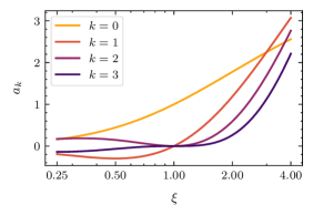
(a) Values for the expansion coefficients $a_{k}$

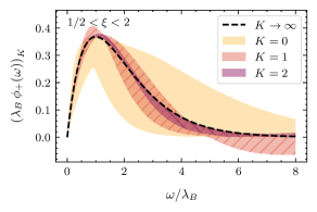
(b) Variability of the momentum-space LCDA for different truncations $K$ in the interval $1/2<\xi<2$.

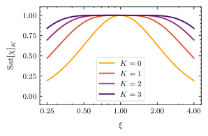
(c) Saturation of the integral bound $\chi$

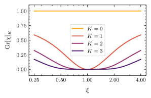
(d) Relative growth of the integral bound $\chi$

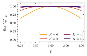
(e) Saturation of the inverse moment $L_{0}=\lambda_{B}^{-1}$.

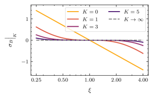
(f) Value of $\sigma_{B}$ for different truncations $K$.

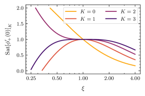
(g) Saturation of the derivative of $\phi_{+}(\omega)$ at the origin.

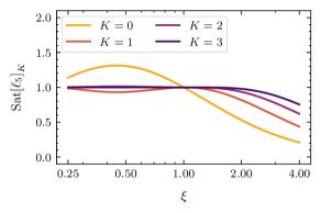
(h) Saturation of the normalized Laplace transform $\ell_{5}$

Figure 2: Plots illustrating the truncation effects of our parametrization for the exponential model Eq. (80). We often use the ratio $\xi=\omega_{0}/\lambda_{B}$, plotted on a logarithmic scale.

The integral bound for the exponential model can be calculated explicitly, yielding a monotonous function of $\xi$,

$$2\omega_{0}\chi=\frac{1}{2}\left(\xi+\xi^{3}\right)\qquad\mbox{[exp.\ model]}\,.$$ (83)

We plot its saturation and its relative growth as a function of $\xi$ in Fig. 2c and Fig. 2d, respectively, for different values of the truncation $K$. We observe that both the saturation and the relative growth give comparable information about the convergence of the parametrization. As expected, the convergence is very rapid as long as $\xi\simeq 1$: taking $K=2$ and varying in the benchmark interval Eq. (82), the saturation exceeds $98\%$ and the relative growth is smaller than $7\%$.

We continue to investigate the saturation for the inverse moment $L_{0}=\lambda_{B}^{-1}$, which is plotted in Fig. 2e. This quantity also rapidly convergences within our parametrization: for $K=2$ the saturation within the benchmark interval is better than $98\%$. It is also instructive to study the normalized first logarithmic moment, which in the model is given by zero at the given scale $\mu_{m}$,

$$\sigma_{B} =0\qquad\mbox{[exp.\ model]}\,.$$ (84)

We show the result as a function of $\xi$ for different truncations $K$ in Fig. 2f. The model result is rapidly reproduced by the truncated parametrization, and the absolute difference falls below $0.11$ for $K=2$ in the benchmark interval.

Finally, we study the saturation of the derivative of the LCDA at the origin $\omega=0$ and of the normalized Laplace transform at $n=\zeta\lambda_{B}$. These test how well our parametrization captures the behavior of the LCDA at small light-cone momentum. In the exponential model, they read:

$$\phi_{+}^{\prime}(0,\mu_{0}) =\lim_{n\to\infty}\ell_{n}=\frac{1}{\lambda_{B}^{2}}\,,\quad\ell_{n}(\mu_{0},1/\lambda_{B})=\frac{1}{\lambda_{B}^{2}}\,\frac{n^{2}}{(1+n)^{2}}\,\qquad\mbox{[exp.\ model]}\,.$$ (85)

In Fig. 2g and Fig. 2h we show the saturation of $\phi_{+}^{\prime}(0)$ and $\ell_{5}$, respectively, for a number of different truncations $K$. We find for $K=2$ in the benchmark interval $0.88<\mathrm{Sat}\left[\phi^{\prime}_{+}(0)\right]_{K}<1.19$ and $0.93<\mathrm{Sat}\left[\ell_{5}\right]_{K}<1.02$. Because of the exponential decrease of the individual coefficients $a_{k}$ in Eq. (81), even $\phi_{+}^{\prime}(0)$ shows a reasonable convergence. As discussed in Section III.2, the convergence of $\ell_{5}$ is expected to be more rapid than for $\phi_{+}(0)$, which is confirmed by the plot.

We conclude that our parametrisation captures the exponential model with high precision even for small $K$. We remark that the parametrisation to any order envelopes the model by construction; however, the dependence on the auxiliary parameter $\omega_{0}$ becomes weaker for growing $K$. We find that $K=2$ offers sufficient precision for practical applications using the model.
Of course, an exemplary behavior of the relatively simple exponential model is expected, since it can be expressed to trivial order in $K$ for the specific choice of $\omega_{0}=\lambda_{B}$. Nevertheless, our analysis provides important input for the comparison with other models in the literature. For that comparison, the exponential model provides a benchmark.

IV.2 Lee-Neubert Model with Radiative Tail

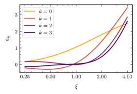
(a) Values for the expansion coefficients $a_{k}$.

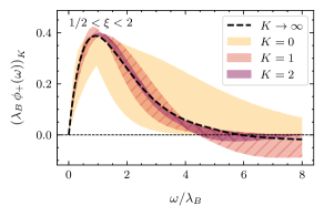
(b) Variability of the momentum-space LCDA for different truncations $K$ in the interval $1/2<\xi<2$.

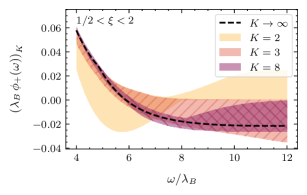
(c) Extension of 3b.

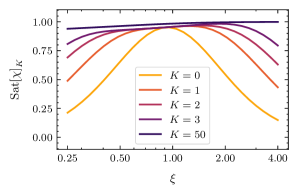
(d) Saturation of the integral bound $\chi$.

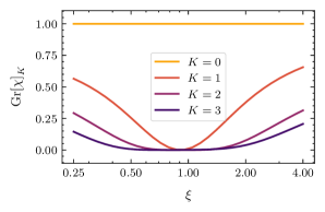
(e) Relative growth of the integral bound $\chi$.

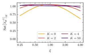
(f) Saturation of the inverse moment $L_{0}=\lambda_{B}^{-1}$.

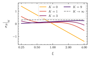
(g) Value of $\sigma_{B}$ for different truncations $K$.

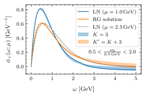
(h) Demonstration of the RG evolution.

Figure 3: Plots illustrating the truncation effects of our parametrization for the Lee-Neubert model Eq. (86). We use the ratio $\xi=\omega_{0}/\lambda_{B}$, plotted on a logarithmic scale.

Lee and Neubert Lee and Neubert (2005) have refined the exponential model by attaching a “radiative tail”, which can be deduced from the behavior of the partonic LCDA at large light-cone momenta $\omega\sim\mu\gg\Lambda_{\rm QCD}$. In this model, the LCDA is described by an exponential at low values of $\omega$, while a radiative tail is added at some intermediate value $\omega_{t}$,

$$\phi_{+}(\omega,\mu_{0}) =\mathcal{N}\,\frac{\omega\,e^{-\omega/\bar{\omega}}}{\bar{\omega}^{2}}+\frac{\alpha_{s}C_{F}}{\pi}\,\frac{\theta(\omega-\omega_{t})}{\omega}\left\{\frac{1}{2}-\ln\frac{\omega}{\mu}+4\,\frac{\bar{\Lambda}_{\rm DA}}{3\omega}\left(2-\ln\frac{\omega}{\mu}\right)\right\}\qquad\text{[Lee/Neubert]}\,.$$ (86)

Here $\bar{\Lambda}_{\text{DA}}$ is the HQET mass parameter in a convenient renormalon-free scheme, see Ref. Lee and Neubert (2005) for details. The parameter $\omega_{t}$ is fixed by requiring the model LCDA to be continuous at $\omega=\omega_{t}$, while the values for ${\cal N}$ and $\bar{\omega}$ are fixed by matching to the partonic calculation. We stress that this model is not supposed to give the correct description at asymptotically large values $\omega\gg\mu$, which would require to further resum the large logarithms $\ln\omega/\mu$ in the above formula (see e.g. the discussion in Ref. Feldmann et al. (2014)). With this in mind, we match our parametrization to this model, and we aim at a reasonable description for small and intermediate values of $\omega$. For the following numerical discussion, we adapt the parameter values found in Ref. Lee and Neubert (2005) for $\mu_{0}=1$ GeV,

$$\bar{\Lambda}_{\rm DA}=519~{}{\rm MeV}\,,\quad\bar{\omega}=438~{}{\rm MeV}\,,\quad{\cal N}=0.963\,,\quad\omega_{t}=2.33~{}{\rm GeV}\,,$$

with $\alpha_{s}(\mu_{0})=0.5$. For this choice one finds

$$L_{0}=\lambda_{B}^{-1}=1/479~{}\text{MeV}^{-1}\,,\qquad\sigma_{B}=0.315\qquad\mbox{[Lee/Neubert]}\,,$$ (87)

and the expansion coefficients $a_{k}$ can easily be calculated numerically. For instance, for $\xi=1$ we find

$$a_{0}\simeq 1.050\,,\quad a_{1}\simeq 0.096\,,\quad a_{2}\simeq-0.007\,,\quad a_{3}\simeq 0.035\,,\quad a_{4}\simeq-0.051\,,\quad a_{5}\simeq 0.047\,.$$

For large values of $k$ the coefficients $a_{k}$ remain almost constant in magnitude, however, with alternating signs. The result for $a_{0},\dots,a_{5}$ and the corresponding approximation to the Lee/Neubert model are shown in Fig. 3a and Fig. 3b, respectively. At first glance, the results look qualitatively very similar to the exponential model. However, the features induced by the radiative tail, namely the cusp at $\omega=\omega_{t}$ and the zero at $\omega\simeq 2.82$ GeV, require special attention. We therefore zoom into the region $4<\omega/\lambda_{B}<12$ in Fig. 3c, where we also consider larger values for the truncation parameter $K$. We find that a reasonably precise description of the radiative tail at intermediate values of $\omega$ requires somewhat higher truncation levels than the exponential model. Note that – by construction – our parametrization is not designed to capture the radiative tail at values $\omega\gg\mu$. We will revisit this point later in Section V.

We continue with the discussion of the integral bound, which in the Lee-Neubert model takes the numerical value

$$2\omega_{0}\chi =0.547\,\xi+0.608\,\xi^{3}\qquad\mathrm{[Lee/Neubert]}\,,$$ (88)

which is close to the exponential model. We emphasize that the bound is finite due to the continuity of the model, despite the derivative in Eq. (51) acting on the Heaviside distribution. The saturation and the relative growth of the integral bound are plotted in Fig. 3d and Fig. 3e, respectively. First, we observe that the saturation is always smaller than one; this is clear, as the bound is monotonously increasing with $K$. Second, we observe that the curves are tilted in comparison to the exponential model: small values of $\xi$ result in slow convergence, while best convergence for the integral bound is obtained for values $\gtrsim 1$. The peaking structure reflects the fact that we need to include terms of higher order in $k$ to get a reasonable description, such that the curve flattens. The relative growth of the bound plotted in Fig. 3e decreases reasonably within our benchmark interval $1/2<\xi<2$.

In Fig. 3f and Fig. 3g, we show the saturation for the inverse moment $L_{0}=\lambda_{B}^{-1}$ and the value of $\sigma_{B}$ as a function of $\xi$ for different levels of truncation, respectively. As in the exponential model, we find good convergence of both quantities in our benchmark interval for $\xi$, with a preference for larger values.

We skip a discussion for $\phi^{\prime}_{+}(0)$ and $\ell_{5}$, which show qualitatively the same behavior as in the exponential model. This is obvious, since they are are naturally only sensitive to the region of small $\omega$, where the radiative tail has no effect.

Next, we use the opportunity to demonstrate the RG evolution of the parameters as defined in Eq. (58). Ref. Lee and Neubert (2005) provides the model parameters for two different choices of the renormalisation scale and plots of the momentum-space LCDA, as well as the general RG solution in momentum space. In Fig. 3h, we show the model at $\mu=1~{}\mathrm{GeV}$ and its RG evolution to $\mu=2.5~{}\mathrm{GeV}$. They coincide well with our truncated parametrization with $K=3$ at the initial scale and its evolution to $\mu=2.5\,\text{GeV}$ with $K^{\prime}=K+3$, using the usual benchmark interval for $\xi=\omega/\lambda_{B}$ for illustration. We also plot the model as provided at $\mu=2.5~{}\mathrm{GeV}$ purely for reference. Our plot is visually indistinguishable from the plots shown in Ref. Lee and Neubert (2005). We further observe that the variation band is consistent for both scales, which verifies the expectation that higher orders in the expansion remain negligible.

IV.3 Naïve Parton Model

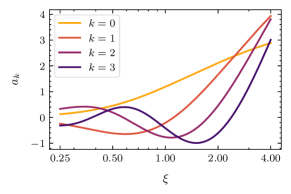
(a) Values for the expansion coefficients $a_{k}$.

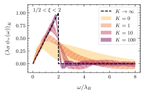
(b) Variability of the momentum-space LCDA for different truncations $K$ in the interval $1/2<\xi<2$.

(c) Saturation of the integral bound $\chi$.

(d) Relative growth of the integral bound $\chi$.

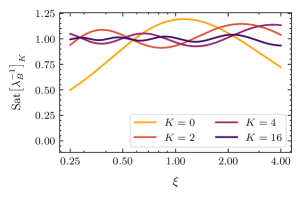
(e) Saturation of the inverse moment $L_{0}=\lambda_{B}^{-1}$.

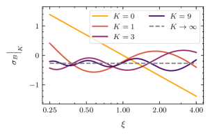
(f) Value of $\sigma_{B}$ for different truncations $K$.

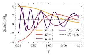
(g) Saturation of the derivative of $\phi_{+}(\omega)$ at the origin.

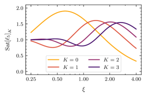
(h) Saturation of the normalized Laplace transform $\ell_{5}$.

Figure 4: Plots illustrating the truncation effects of our parametrization for the parton model Eq. (89). We often use the ratio $\xi=\omega_{0}/\lambda_{B}$, plotted on a logarithmic scale.

In the naïve parton model Kawamura et al. (2001) the LCDA takes the form

$$\phi_{+}(\omega)=\frac{\omega}{2\lambda_{B}^{2}}\,\theta(2\lambda_{B}-\omega)\qquad\mbox{[parton model]}\,,$$ (89)

where $\lambda_{B}$ is identified with the HQET mass parameter $\bar{\Lambda}\simeq M_{B}-m_{b}$. In position space this yields

$$\tilde{\phi}_{+}(\tau) =\frac{(1+2i\lambda_{B}\tau)\,e^{-2i\lambda_{B}\tau}-1}{2\lambda_{B}^{2}\tau^{2}}\qquad\mbox{[parton model]}\,,$$ (90)

which only falls off as $1/\tau$ for $|\tau|\to\infty$, thereby violating P4. The parton-model LCDA is therefore a pathological example of a model. Nevertheless, it can serve as a toy model to study under which circumstances our parametrization can also capture extreme examples.

To this end, we show the numerical result for the expansion coefficients and the resulting shapes of the momentum-space LCDA for different levels of truncation in Fig. 4a and Fig. 4b, respectively. Indeed, we observe that the expansion coefficients remain sizable even for large values of $k$, without any preferred value for the ratio $\xi$. This indicates a bad convergence of the expansion. Similarly, our estimate for the truncation uncertainty in Fig. 4b, reflected by the variation of $\xi$ in the benchmark interval, is larger than in the exponential model. As expected, the triangular shape cannot be reproduced well, even for very high levels of truncation.

As $\tilde{\phi}(\tau)$ only falls off as $1/\tau$, the integral bound $\chi$ in Eq. (27) does not exist for our choice of the function $r(\tau,\mu_{0})$. In Fig. 4c we therefore only plot the diverging sum

$$2\omega_{0}\chi\big{|}_{K}=\sum_{k=0}^{K}|a_{k}|^{2}\,,$$

together with its relative growth in Fig. 4d. The observed oscillatory behavior of the latter can be taken as an indicator for the non-convergence of the expansion.

We continue with the discussion of $L_{0}=\lambda_{B}^{-1}$ for which we plot the saturation in Fig. 4e. Its saturation oscillates around unity with an amplitude that is only slowly decreasing with increasing $K$. The normalized first logarithmic moment is given by

$$\sigma_{B} =1-\ln 2-\gamma_{\text{E}}\simeq-0.270\qquad\mbox{[parton model]}\,.$$ (91)

In Fig. 4f we show the result for different truncation $K$. Again we observe an oscillatory behavior around the true model value.

Finally, we study the convergence of our parametrization at low values of $\omega$. We obtain

$$\phi_{+}^{\prime}(0,\mu_{0})=\frac{1}{2\lambda_{B}^{2}}\,,\qquad\ell_{n}(\mu_{0},1/\lambda_{B})=\frac{1}{2\lambda_{B}^{2}}\left(1-(1+2n)\,\mathrm{e}^{-2n}\right)\qquad\mbox{[parton model]}\,.$$ (92)

The saturation of the derivative at the origin in Fig. 4g shows oscillatory behavior for the whole range of $\xi$, while for the normalized Laplace transform we observe that the saturation in Fig. 4h approaches unity for sufficiently large values of $K$ and/or small values of $\xi$.

IV.4 A Model with $\phi_{+}^{\prime}(0)\to\infty$

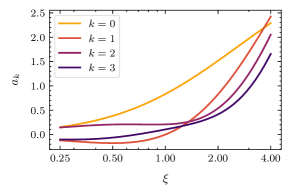
(a) Values for the expansion coefficients $a_{k}$.

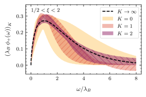
(b) Variability of the momentum-space LCDA for different truncations $K$ in the interval $1/2<\xi<2$.

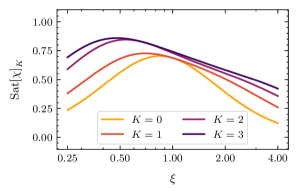
(c) Saturation of the integral bound $\chi$.

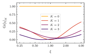
(d) Relative growth of the integral bound $\chi$.

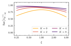
(e) Saturation of the inverse moment $L_{0}=\lambda_{B}^{-1}$.

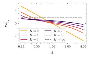
(f) Value of $\sigma_{B}$ for different truncations $K$.

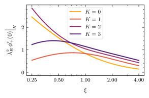
(g) Partial sum of the derivative at the origin.

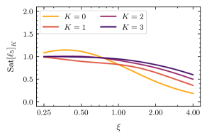
(h) Saturation of the normalized Laplace transform $\ell_{5}$.

Figure 5: Plots illustrating the truncation effects of our parametrization for the model Eq. (93) discussed by Beneke et al. Beneke et al. (2018). We often use the ratio $\xi=\omega_{0}/\lambda_{B}$, plotted on a logarithmic scale.

Beneke et al. Beneke et al. (2018) have suggested to consider more general parametrizations for the $B$-meson LCDA, which also include cases where the derivative at the origin $\phi_{+}^{\prime}(0)$ does not exist. We study their model

$$\phi_{+}(\omega,\mu_{0}) =\frac{1}{\Gamma(1+a)}\,\left(\frac{(1+a)\,\omega}{\lambda_{B}}\right)^{1+a}\frac{\mathrm{e}^{-(1+a)\,\omega/\lambda_{B}}}{\lambda_{B}}\quad\mbox{[Beneke et al.]}\,.$$ (93)

For $a\to 0$, this function reduces to the simple exponential model. For $a<0$, the behavior at $\omega\to 0$ is somewhat pathological, since it violates P4. Nevertheless, it is interesting to study the convergence of our parametrization for this behavior. For concreteness, in the following we only consider the case $a=-0.4$.

We show the coefficients $a_{k}$ and the resulting shapes to the LCDA for different levels of truncation in Fig. 5a and Fig. 5b, respectively. We see that except for the vicinity of $\omega=0$, already $K=2$ yields a reasonable approximation within the estimated uncertainty from the $\xi$-variation.

The integral bound for the model follows as

$$2\omega_{0}\chi =\frac{1}{2^{1+2a}}\,\frac{\Gamma(2+2a)}{\Gamma(1+a)^{2}}\left(\xi+\frac{(1+a)^{2}}{1+2a}\,\xi^{3}\right)\overset{a\to-0.4}{\simeq}0.360\,\xi+0.649\,\xi^{3}\qquad\mbox{[Beneke et al.]}\,.$$ (94)

In Fig. 5c we observe the opposite behavior as compared to the Lee-Neubert model, i.e. the peak of the saturation is tilted to the other side, such that the best convergence is obtained for small values of $\xi$. Again, the relative growth of the integral bound in Fig. 5d remains small in the benchmark interval around $\xi=1$.

The saturation of the inverse moment $L_{0}=\lambda_{B}^{-1}$ and the normalized first logarithmic moment,

$$\sigma_{B}=-\Psi(1+a)+\ln(1+a)-\gamma_{\text{E}}\overset{a\to-0.4}{\simeq}+0.453\qquad\mbox{[Beneke et al.]}\,,$$ (95)

are shown in Fig. 5e and Fig. 5f, respectively. Compared to the exponential model shown in Fig. 2e, the saturation for $L_{0}$ converges more slowly, and the truncated result for $\sigma_{B}$ is rather sensitive to the value of $\xi$ (for moderate truncation $K$).
The fact that $\sigma_{B}$ can be adjusted by an independent parameter $a$ may be viewed as an advantage of the model Eq. (93). However the required pathological behavior at $\omega\to 0$ makes it less useful in phenomenological applications. We therefore advocate our parametrization, which is able to systematically decorrelate the pseudo observables by including sufficiently many terms. We illustrate this point in the following section.

Finally, we also show the results for the quantities that characterize the behavior of the LCDA at small values of $\xi$. As the derivative at the origin does not exist in the model (93), in Fig. 5g we only show the truncated sum for a finite value of $K$,

$$\phi_{+}^{\prime}(0)_{K}=\frac{1}{\omega_{0}^{2}}\,\sum_{k=0}^{K}a_{k}\,.$$

Indeed, no convergence is apparent. In Fig. 5h, we show the saturation of the normalized Laplace transform,

$$\ell_{n}(\mu_{0},1/\lambda_{B})=\frac{n^{2}}{\lambda_{B}^{2}}\left(\frac{1+a}{n+1+a}\right)^{2+a}\qquad\mbox{[Beneke et al.]}\,,$$ (96)

at $n=5$. Here, we observe similarly good saturation properties as for the exponential model.

V Pseudo-phenomenology

In this section we illustrate the feasibility of using our parametrization to describe the LCDA in its full kinematic range, based on a global analysis of all available phenomenological information in the future. Here, we do not strive for a rigorous statistical analysis. Instead, we illustrate the complementarity of the available constraints in a qualitative manner. Quantitative statements herein should not be mistaken for theoretical predictions.

V.1 Using $\lambda_{B}$ and $\ell_{5}$ as Phenomenological Constraints

In this subsection we study the hypothetical situation that some phenomenological information, be it experimental or theoretical in nature, constrains the quantities (“pseudo observables”)

$$p_{1}\equiv L_{0}(\mu_{0},\mu_{m})\qquad\mbox{and}\qquad p_{2}\equiv\lambda_{B}^{2}\,\ell_{5}(\mu_{0},1/\lambda_{B})$$ (97)

at a low reference scale $\mu_{0}$. We select these two pseudo observables, because they emerge in the theoretical description of the $\bar{B}^{-}\to\gamma\mu^{-}\bar{\nu}$ form factors. An experimental determination of the these form factors, through measurements of the decays, is foreseen by the Belle II experiment Heller et al. (2015); Gelb et al. (2018); Altmannshofer et al. (2019). Moreover, these two pseudo observables probe complementary aspects of the $B$-meson LCDA: in the following discussion we will neglect the uncertainties on these parameters for simplicity. Of course, in a realistic fit to experimental data, these uncertainties as well as their correlations have to be taken into account. With no further theory input at hand, we can use our parametrization to estimate the effect on the $B$-meson LCDA and other derived quantities.

Here, we truncate at $K=2$, which yields four independent parameters. They are $\omega_{0}$ and $a_{0}$ through $a_{2}$. With the two phenomenological constraints above, we can determine two of these parameters. We choose to determine $a_{0}$ and $a_{1}$:

$$a_{0} =\xi-\frac{a_{2}}{3}\,, a_{1} =\frac{(5\xi+1)^{3}}{25\,(5\xi-1)}\,p_{2}-\frac{\xi\,(5\xi+1)}{5\xi-1}-\frac{2\,(25\xi^{2}-20\xi+1)}{3(5\xi+1)(5\xi-1)}\,a_{2}\,, \text{where }\xi =p_{1}\,\omega_{0}\,.$$ (98)

This leaves two unconstrained parameters: the auxiliary scale ratio $\xi$ and the coefficient $a_{2}$. In order to constrain the possible ranges for $\xi$ and $a_{2}$, we now impose the following conditions, which are motivated by the findings in the previous subsection: The relative growth of the integral bound $\chi$ is limited to $20\%$ (for $K=1$) and $10\%$ (for $K=2$),

$$\frac{|a_{1}|^{2}}{|a_{0}|^{2}+|a_{1}|^{2}} \leq 0.2\,, \frac{|a_{2}|^{2}}{|a_{0}|^{2}+|a_{1}|^{2}+|a_{2}|^{2}} \leq 0.1\,.$$ (99)

Combined with Eq. (98) this provides a bounded region for the joint distribution of the parameters $\xi$ and $a_{2}$. For any given pseudo observable we can therefore determine its minimal and maximal values for parameter values in that region.

For example, the result for the normalized logarithmic moment at the reference scale $\mu_{m}=1/p_{1}\,e^{-\gamma_{E}}$ is given by

$$\sigma_{B}\big{|}_{2}\equiv-\frac{1}{p_{1}}\,L_{1}(\mu_{0},1/p_{1}\,\mathrm{e}^{-\gamma_{E}})\Big{|}_{K=2}=-\ln\xi+\frac{a_{1}}{\xi}\,.$$ (100)

In the following, we will determine the resulting variations for the normalized logarithmic moment $\sigma_{B}$ at $K=2$, as well as for the LCDA $\phi(\omega)$ at different values of $x=\omega\,p_{1}$, and the normalized Laplace transformation $\ell_{n}$ at different (real) values of $n$ for each of the four models discussed in Section IV. Note that at this stage, the only difference between the four models is given by their predictions for the pseudo-observable $p_{2}$, while the pseudo-observable $p_{1}$ only enters via the auxiliary parameter $\xi$ to set the reference scale in the analysis.

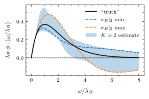
(a) Using the exponential model Eq. (80).

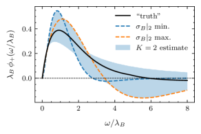
(b) Using the Lee-Neubert model Eq. (86).

Figure 6: Pseudo-fit to the $B$-meson LCDA in momentum space using the two pseudo-observables $p_{1,2}$ as predicted by two models as a function of $x=\omega/\lambda_{B}$. We show the model (“truth”), the curves that lead to extreme values of $\sigma_{B}$ and the total variation of the parametrized LCDA. For the latter, we take the benchmark interval for $\xi=\omega_{0}/\lambda_{B}$ and a small $a_{2}$ into account.

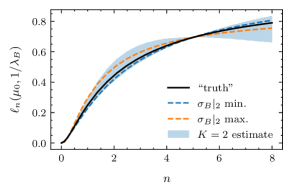
(a) Using the exponential model Eq. (80).

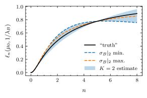
(b) Using the Lee-Neubert model Eq. (86).

Figure 7: Pseudo-fit to the normalized Laplace transform $\ell_{n}(\mu_{0},1/\lambda_{B})$ using the two pseudo-observables $p_{1,2}$ as predicted by two models as a function of $x=\omega/\lambda_{B}$. We show the model (“truth”), the curves that lead to extreme values of $\sigma_{B}$ and the total variation of the parametrized LCDA. For the latter, we take the benchmark interval for $\xi=\omega_{0}/\lambda_{B}$ and a small $a_{2}$ into account.

V.1.1 Exponential Model

In the exponential model Eq. (80) the value for the pseudo-observable $p_{2}$ is given by

$$p_{2}=\frac{25}{36}\simeq 0.694\,,\qquad\text{[exp.\ model]}$$ (101)

from which we can directly determine the coefficients $a_{0}$ and $a_{1}$ in the truncated parametrization. We may now determine the maximal range of values that $\sigma_{B}$ can take, when the free parameters $\xi$ and $a_{2}$ are varied as explained above. This results in

$$\sigma_{B}\big{|}_{2}^{\rm min} =-0.073 \mbox{for $\xi\to 1.332$ and $a_{2}\to+0.410$}\,,$$ (102)

$$\sigma_{B}\big{|}_{2}^{\rm max} =+0.172 \mbox{for $\xi\to 1.489$ and $a_{2}\to-0.625$}\,,$$ (103)

while $\sigma_{B}=0$ in the exponential model. We further plot the momentum space LCDA $\phi_{+}(\omega,\mu_{0})$ and its corresponding Laplace transform $\ell_{n}(\mu_{0},1/\lambda_{B})$ in Fig. 6a and Fig. 7a, respectively, as well as the corresponding curves for the extreme values of $\sigma_{B}$. We find that the parameter values are constrained to the intervals $0.607<\xi<1.499$, $-0.633<a_{2}<0.477$, and $0.607<\xi<1.636$, $-0.632<a_{2}<0.539$, respectively. We observe the following:

1. The knowledge of the pseudo-observables $p_{1}$ and $p_{2}$ indeed fixes the behavior of $\phi_{+}(\omega)$ at low momentum, as well as the behavior of its Laplace transform at large values of $\zeta=-i\tau\gg\lambda_{B}$.

2. The shape of $\phi_{+}(\omega)$ at intermediate values of $\omega$ is very sensitive to the variation of $\xi$ and $a_{2}$, and therefore not very meaningful without additional phenomenological constraints.

3. Similarly, the behavior of the Laplace transform at small values of $\zeta\lesssim 1$ is sensitive to the variation of $\xi$ and $a_{2}$, but in contrast to the LCDA in momentum space, the shape of the Laplace transform remains stable, reflecting a monotonous function (at least, as long as $\zeta$ is not too close to zero).

From this we can already see, that a meaningful fit to the LCDA would benefit from additional information on the Laplace transform at small values of $\zeta$ (i.e. the LCDA in position space at imaginary light-cone time $-i\tau\lesssim\lambda_{B}$). This will be further illustrated below.

V.1.2 Lee-Neubert Model with Radiative Tail

In the Lee-Neubert model Eq. (86) the value for the pseudo-observable $p_{2}$ is given by

$$\quad p_{2}\simeq 0.777\qquad[\text{Lee/Neubert}]\,,$$ (104)

which is slightly larger than for the exponential model. The corresponding ranges for the logarithmic moment are obtained as

$$\sigma_{B}\big{|}_{2}^{\rm min} =0.045 \mbox{for $\xi\to 0.541$ and $a_{2}\to-0.225$}\,,$$ (105)

$$\sigma_{B}\big{|}_{2}^{\rm max} =0.321 \mbox{for $\xi\to 1.283$ and $a_{2}\to-0.543$}\,,$$ (106)

This includes the value $\sigma_{B}\simeq 0.315$ of the LN model. We observe that values of $p_{2}$ that are larger than in the exponential model yield larger values of $\sigma_{B}$. We will discuss how to consistently implement information on the “radiative tail” in a modified fit procedure in Section V.2. We plot the momentum-space LCDA and its Laplace transform in Fig. 6b and Fig. 7b. We find that the parameter values are constrained to the intervals $0.498<\xi<1.342$, $-0.546<a_{2}<0.439$, and $0.540<\xi<1.381$, $-0.536<a_{2}<0.458$, respectively.

V.1.3 Naïve Parton Model

We can repeat the analysis for the naïve parton model. Here the pseudo-observable $p_{2}$ takes the value

$$\quad p_{2}=(1-11\,\mathrm{e}^{-10})/2\simeq 0.5\qquad\text{[parton model]}\,,$$ (107)

which now is smaller than in the exponential model. With this, the range of values that $\sigma_{B}$ can take amounts to

$$\sigma_{B}\big{|}_{2}^{\rm min} =-0.565 \mbox{for $\xi\to 1.810$ and $a_{2}\to+0.543$}\,,$$ (108)

$$\sigma_{B}\big{|}_{2}^{\rm max} =-0.231 \mbox{for $\xi\to 2.228$ and $a_{2}\to-0.943$}\,,$$ (109)

which includes the “true” value $\sigma_{B}\simeq-0.270$ in the naïve parton model. We find that the parameter values are constrained to the intervals $0.824<\xi<2.229$, $-0.948<a_{2}<0.536$, and $0.824<\xi<2.242$, $-0.947<a_{2}<0.697$, respectively. Qualitatively, as before, we observe that now smaller values of $p_{2}$ tend to yield smaller values of $\sigma_{B}$ in the pseudo-fit.

V.1.4 Model with $\phi_{+}^{\prime}(0)\to\infty$

Repeating the analysis for the model Eq. (93), we observe that the value of the pseudo-observable

$$p_{2}\simeq 0.701\qquad[\text{Beneke et al.}]$$ (110)

is very close to that of the exponential model. As a consequence – without further input – the fit cannot distinguish the two cases. Note that the range for the first logarithmic moment that results from our fit procedure will not include the actual value $\sigma_{B}=0.453$ in this model. This can be traced back to the pathological behavior of the model at $\omega\to 0$.

V.2 Adding Theoretical Constraints from the Short-distance OPE

As has previously been mentioned, the $B$-meson LCDA can be constrained using information obtained from the short-distance OPE of the light-cone operator. The latter describes the behavior of $\tilde{\phi}_{+}(\tau)$ at small values of $|\tau|\sim 1/\mu\ll 1/\Lambda_{\text{QCD}}$, and it can be obtained from a fixed-order partonic calculation in HQET Kawamura and Tanaka (2009),

$$\tilde{\phi}_{+}(\tau,\mu) =1-\frac{\alpha_{s}C_{F}}{4\pi}\left(2L^{2}+2L+\frac{5\pi^{2}}{12}\right)-i\tau\,\frac{4\bar{\Lambda}}{3}\left[1-\frac{\alpha_{s}C_{F}}{4\pi}\left(2L^{2}+4L-\frac{9}{4}+\frac{5\pi^{2}}{12}\right)\right]+\mathcal{O}(\tau^{2}\Lambda_{\text{QCD}}^{2})\,.$$ (111)

In the above, $\bar{\Lambda}$ is the HQET mass parameter in the on-shell scheme and we abbreviate

$$L=\ln(i\tau\mu e^{\gamma_{E}})\,.$$

In the Lee-Neubert model Eq. (86) the short-distance information has been added as a radiative tail in momentum space, by considering cut-off moments $M_{n}(\Lambda_{\rm UV})=\int_{0}^{\Lambda_{\rm UV}}d\omega\,\omega^{n}\,\phi_{+}(\omega)$. A more direct and simpler approach is to evaluate the LCDA in position space, using our parametrization, and compare with Eq. (111). To this end, we have to first expand our parametrization in $\omega_{0}/\mu_{0}\ll 1$ for a fixed value of

$$x_{0} \equiv i\tau_{0}\mu_{0}\,e^{\gamma_{E}}\sim{\cal O}(1)$$ (112)

The analogue of the first two moments $M_{0}$ and $M_{1}$ used in the Lee-Neubert model are then taken as the value and first derivative of $\tilde{\phi}_{+}(\tau)$, which defines the two theory inputs

$$t_{1} \equiv\tilde{\phi}(\tau_{0},\mu_{0})\,,\qquad t_{2}\equiv i\frac{d\tilde{\phi}(\tau,\mu_{0})}{d\tau}\bigg{|}_{\tau=\tau_{0}}\,.$$ (113)

Let us first consider a situation where only this theory input is known. A minimal approach would then be to consider our parametrization at truncation level $K=1$ and fix the parameters $a_{0}$ and $a_{1}$ by matching $t_{1}$ and $t_{2}$ to Eq. (111). This yields

$$a_{0} =2-\frac{2\bar{\Lambda}}{3\omega_{0}}+\frac{\alpha_{s}C_{F}}{4\pi}\left(-\frac{1}{x_{0}}\,\frac{\mu_{0}e^{\gamma_{E}}}{\omega_{0}}\,(1+2\ln x_{0})+\ldots\right)\,,$$ (114)

$$a_{1} =1-\frac{2\bar{\Lambda}}{3\omega_{0}}+\frac{\alpha_{s}C_{F}}{4\pi}\left(-\frac{1}{x_{0}}\,\frac{\mu_{0}e^{\gamma_{E}}}{\omega_{0}}\,(1+2\ln x_{0})+\ldots\right)\,,$$ (115)

where we only show the $\alpha_{s}$ corrections that are enhanced by $\mu_{0}/\omega_{0}$. These terms can be absorbed by a redefinition of the HQET mass parameter: For our purpose, a convenient renormalization scheme is

$$\bar{\Lambda} \equiv\bar{\Lambda}_{a}(\mu,x_{0})\left[1+\frac{\alpha_{s}C_{F}}{4\pi}\left(10\,\ln x_{0}+\frac{15}{4}\right)\right]-\frac{\alpha_{s}C_{F}}{4\pi}\,\frac{3\mu e^{\gamma_{E}}}{2x_{0}}\left(1+2\ln x_{0}\right)$$ (116)

which yields

$$a_{0} =Z(x_{0})\left(2-\frac{2\bar{\Lambda}_{a}}{3\omega_{0}}-\frac{8\alpha_{s}C_{F}}{3\pi}\,\frac{\bar{\Lambda}_{a}x_{0}}{\mu_{0}e^{\gamma_{E}}}\,(1+\ln x_{0})\right)\,,$$ (117)

$$a_{1} =Z(x_{0})\left(1-\frac{2\bar{\Lambda}_{a}}{3\omega_{0}}-\frac{4\alpha_{s}C_{F}}{3\pi}\,\frac{\bar{\Lambda}_{a}x_{0}}{\mu_{0}e^{\gamma_{E}}}\,(1+\ln x_{0})\right)\,,$$ (118)

with

$$Z(x_{0}) =1+\frac{\alpha_{s}C_{F}}{4\pi}\left(-2\ln^{2}x_{0}+2\ln x_{0}+2-\frac{5\pi^{2}}{12}\right)\,.$$ (119)

Our definition of $\bar{\Lambda}_{a}$ and $Z(x_{0})$ have been chosen such that the result for the position-space LCDA with finite truncation $K$ always satisfies

$$\tilde{\phi}_{+}(0)\big{|}_{K} =\sum_{k=1}^{K}(-1)^{k}\,a_{k}=Z(x_{0})-\frac{4\alpha_{s}C_{F}}{3\pi}\,\frac{\bar{\Lambda}_{a}x_{0}}{\mu_{0}e^{\gamma_{E}}}\,(1+\ln x_{0})\,,$$ (120)

$$\tilde{\phi}_{+}^{\prime}(0)\big{|}_{K} =-2i\omega_{0}\,\sum_{k=1}^{K}(-1)^{k}\,(1+k)\,a_{k}=-Z(x_{0})\,\frac{4i\bar{\Lambda}_{a}}{3}\,,$$ (121)

which generalizes the Grozin-Neubert relations in Ref. Grozin and Neubert (1997) to one-loop accuracy in our formalism. It is instructive to compare with the approach by Lee and Neubert in Ref. Lee and Neubert (2005), where corresponding expressions are obtained for the zeroth and first moment of the momentum-space LCDA with a UV cut off. The perturbative relation between the parameter $\bar{\Lambda}_{\text{DA}}$ defined in that scheme and our scheme reads

$$\bar{\Lambda}_{a}(\mu,x_{0}) =\bar{\Lambda}_{\rm DA}(\mu,\mu)\left[1+\frac{\alpha_{s}C_{F}}{4\pi}\left(-10\,\ln x_{0}-2\right)\right]+\mu\,\frac{\alpha_{s}C_{F}}{4\pi}\left(\frac{3e^{\gamma_{E}}}{2x_{0}}\,(1+2\ln x_{0})-\frac{9}{2}\right)\,.$$ (122)

For instance, using $x_{0}=1$, $\mu_{0}=1\,$\mathrm{GeV}$$, $\bar{\Lambda}_{\rm DA}(\mu_{0},\mu_{0})=519$ MeV, and $\alpha_{s}(\mu_{0})=0.5$ as in Ref. Lee and Neubert (2005), we obtain

$$\bar{\Lambda}_{a}(\mu_{0},x_{0})=367\,\text{MeV}\,.$$

We are now in the position to include the phenomenological constraints $p_{1}$ and $p_{2}$ as defined in the previous subsection. For the sake of legibility, we introduce the quantity

$$n_{0}\equiv i\tau_{0}\omega_{0}=\frac{x_{0}\omega_{0}}{\mu_{0}e^{\gamma_{E}}}\,.$$ (123)

For the power expansion defined by the OPE to converge, we would need $x_{0}\sim{\cal O}(1)$ and small values of $n_{0}$. On the other hand, the (reasonably fast) convergence of our parametrization requires a finite $n_{0}>0$. In the following, we use

$$n_{0}=1/3\,,\quad\mu_{0}=1~{}{\rm GeV}\,,$$

as our default choice, while the value of $\omega_{0}$ (and thus of $x_{0}$) will be varied within the fit, with suitable constraints on the resulting relative growth (see below). For instance, a value $x_{0}=1$ corresponds to $\omega_{0}\approx 600$ MeV, which appears reasonable. Note that our choice for $n_{0}$ corresponds to the value $y_{0}=-1/2$ in Eq. (28), which lies exactly halfway between the origin and the local limit ($y=-1$).

With two new constraints we increase the truncation level from $K=2\to 4$ compared to the previous subsection, leaving $a_{4}(\mu_{0})$ and $\xi=\omega_{0}/\lambda_{B}$ as free parameters. For $\xi=1$ and $x_{0}=1$ we obtain

$$a_{0} =Z\left(-\frac{28}{25}+\frac{2\bar{\Lambda}_{a}p_{1}}{15}\right)+\frac{112\alpha_{s}C_{F}}{75\pi}\,\bar{\Lambda}_{a}n_{0}p_{1}+3-\frac{972\,p_{2}}{625}-\frac{4a_{4}}{15}\,,$$ (124)

$$a_{1} =Z\left(-2+\frac{\bar{\Lambda}_{a}p_{1}}{3}\right)+\frac{8\alpha_{s}C_{F}}{3\pi}\,\bar{\Lambda}_{a}n_{0}p_{1}+\frac{3}{2}-\frac{4a_{4}}{5}\,,$$ (125)

$$a_{2} =Z\left(\frac{84}{25}-\frac{2\bar{\Lambda}_{a}p_{1}}{5}\right)-\frac{112\alpha_{s}C_{F}}{25\pi}\,\bar{\Lambda}_{a}n_{0}p_{1}-6+\frac{2916\,p_{2}}{625}+\frac{a_{4}}{5}\,,$$ (126)

$$a_{3} =Z\left(\frac{81}{25}-\frac{3\bar{\Lambda}_{a}p_{1}}{5}\right)-\frac{108\alpha_{s}C_{F}}{25\pi}\,\bar{\Lambda}_{a}n_{0}p_{1}-\frac{9}{2}+\frac{1944\,p_{2}}{625}+\frac{26a_{4}}{15}\,,$$ (127)

where $Z\equiv Z(x_{0}=1)$. The result for arbitrary values of $\xi$ and $x_{0}$ can be found in Appendix B. The parameter range for $a_{4}$ and $\xi$ will be further constrained by analogous conditions on the relative growth as in the previous subsection,

$${\rm Gr}[\chi]_{K}\leq\frac{20\%}{K}$$ (128)

which generalizes Eq. (99).

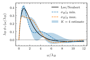
(a) Momentum-space LCDA.

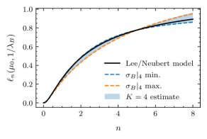
(b) Laplace transform $\ell_{n}$.

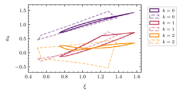
(c) Bounded regions for each parameter.

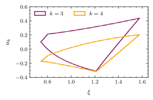
(d) Bounded regions for each parameter.

Figure 8: Results from the pseudo-fit employing theoretical constraints in addition to the phenomenological inputs $p_{1}$ and $p_{2}$. The dashed regions in Fig. 8c correspond to the pseudo-fit without theoretical OPE constraints.

Among the four benchmark models discussed in Section IV, only the Lee-Neubert model in Eq. (86) features a radiative tail that reflects the constraints from the local OPE. We therefore consider this model as a benchmark. We expect that the pseudo-fit should correctly reproduce the main qualitative and quantitative features of that model. We therefore set

$$p_{1}=1/\lambda_{B}=2.085\,\text{GeV}^{-1}\,,\quad p_{2}=0.777\qquad[\text{Lee/Neubert}]\,,$$ (129)

and take the same input for the theory parameters as outlined below Eq. (86), while $\bar{\Lambda}_{a}$ is calculated from Eq. (122) as a function of $x_{0}$. As in Section V, we consider the normalized first logarithmic moment, now truncated at $K=4$,

$$\sigma_{B}\big{|}_{4}=-\ln\xi+\frac{a_{1}+2/3\,a_{3}}{\xi}\,.$$ (130)

We find the following range of values, constrained by the growth criterion,

$$\sigma_{B}\big{|}_{4}^{\rm min} =0.114 \mbox{for $\xi\to 0.961$ and $a_{2}\to-0.232$}\,,$$ (131)

$$\sigma_{B}\big{|}_{4}^{\rm max} =0.217 \mbox{for $\xi\to 0.905$ and $a_{2}\to-0.030$}\,.$$ (132)

This interval is compatible with the estimate obtained by using only $p_{1}$ and $p_{2}$. However, its size is reduced by more than $60\,\%$. The value $\sigma_{B}=0.315$ in the Lee/Neubert model is not contained in this estimate.

We show the resulting momentum-space LCDA and Laplace transform in Fig. 8a and Fig. 8b, respectively, where we find that the parameters are restricted as $0.745<\xi<1.577$, $-0.319<a_{4}<0.201$, and $0.743<\xi<1.522$, $-0.312<a_{4}<0.120$. In Fig. 8c, we compare the allowed regions for the coefficients $a_{0}$ through $a_{2}$ obtained here with the ones as obtained in Section V. We find that the regions largely overlap, while shrinking significantly for $a_{0}$ and $a_{2}$ and staying approximately constant for $a_{1}$. We further show the regions for the additional coefficients $a_{3}$ and $a_{4}$ in Fig. 8d.

Once more, we caution that the plots and numerical results here illustrate the applicability of our method. However, they cannot be interpreted as predictions, which would require a more careful treatment of uncertainties on the basis of experimental data.

VI Conclusion and Outlook

We have proposed a novel systematic parametrization of the leading-twist $B$-meson light-cone distribution amplitude (LCDA) in position space. At the center of our derivation is the Taylor expansion of the LCDA in a conveniently chosen variable $y$, which arises from the conformal transformation in Eq. (28). The coefficients of that expansion obey an integral bound Eq. (34), which provides qualitative control of the truncation error of the expansion, with the numerical value of the bound presently unknown. Our parametrization yields simple expressions for a variety of quantities connected to the LCDA, including its logarithmic moments and a set of “pseudo-observables” describing the low-momentum behavior. For convenience we summarize the resulting formulas for the most important functions in Table 1. We have also discussed three different approaches to implement the renormalization-group (RG) evolution of the LCDA and its derived quantities within our framework. We have identified one approach that allows a computationally efficient implementation in future phenomenological analyses.

We have performed detailed numerical studies to show that our parametrization can successfully reproduce different benchmark models, including non-trivial features like the ”radiative tail” at large light-cone momentum. Furthermore, we have illustrated the power of our approach to combine different types of phenomenological and theoretical constraints. This is achieved through matching our parametrization to hypothetical values of two “pseudo-observables” in Eq. (97) that are expected to be constrained by future experimental data on the photo-leptonic $B\to\gamma\ell\nu$ decay. Moreover, we have shown that theoretical constraints on the expansion parameters from the local operator product expansion (OPE) can be implemented at small but finite light-cone separation in a natural and straight-forward manner. We have used this to define a new renormalization scheme Eq. (116) for the mass parameter in heavy-quark effective theory (HQET), which resembles the so-called “DA-scheme” that has been introduced by Lee and Neubert from the consideration of “cut-off” moments.

Our framework is general enough to allow theoretical refinements in the future. First, it can be applied to higher-twist LCDA of the $B$-meson, as we have briefly discussed for the Wandzura-Wilczek part of the twist-three LCDA $\phi_{-}$. Second, the available two-loop RG evolution can be implemented on the level of our truncated expansion. Third, the OPE constraints from dimension-five HQET operators can be included as well. Finally, on the phenomenological side, a future determination of the very value of the integral bound, e.g. from lattice QCD studies, would allow us to quantify the truncation errors.

position-space LCDA	$\displaystyle\tilde{\phi}_{+}(\tau,\mu_{0})$	$\displaystyle=$	$\displaystyle\frac{1}{(1+i\omega_{0}\tau)^{2}}\,\sum\limits_{k=0}^{K}a_{k}(\mu_{0})\left(\frac{i\omega_{0}\tau-1}{i\omega_{0}\tau+1}\right)^{k}$
momentum-space LCDA	$\displaystyle\phi_{+}(\omega,\mu_{0})$	$\displaystyle=$	$\displaystyle\frac{\omega\,e^{-\omega/\omega_{0}}}{\omega_{0}^{2}}\,\sum\limits_{k=0}^{K}a_{k}(\mu_{0})\,\frac{1}{1+k}\,L_{k}^{(1)}(2\omega/\omega_{0})$
dual-space LCDA	$\displaystyle\eta_{+}(s,\mu_{0})$	$\displaystyle=$	$\displaystyle e^{-s\omega_{0}}\,\sum\limits_{k=0}^{K}a_{k}(\mu_{0})\,\frac{(-1)^{k}}{1+k}\,L_{k}^{(1)}(2\omega_{0}s)$
generating function	$\displaystyle F_{[\eta_{+}]}(t;\mu_{0},\mu_{m})$	$\displaystyle=$	$\displaystyle\frac{\Gamma(1-t)}{\omega_{0}}\,\left(\frac{\hat{\mu}_{m}}{\omega_{0}}\right)^{-t}\,\sum\limits_{k=0}^{K}a_{k}(\mu_{0})\,{}_{2}F_{1}(-k,1+t,2,2)$
inverse moment	$\displaystyle\lambda_{B}^{-1}(\mu_{0})$	$\displaystyle=$	$\displaystyle\frac{1}{\omega_{0}}\,\sum\limits_{k=0}^{K}a_{k}(\mu_{0})\,\frac{1+(-1)^{k}}{2\,(1+k)}$   (only even $k$)
logarithmic moment	$\displaystyle\sigma_{B}(\mu_{0})$	$\displaystyle=$	$\displaystyle-\ln\xi-\frac{1}{\xi}\,\sum_{k=0}^{K}a_{k}(\mu_{0})\left[\derivative{t}\,{}_{2}F_{1}(-k,1+t;2;2)\right]_{t=0}$   (only odd $k$)
derivative at $\omega=0$	$\displaystyle\phi_{+}^{\prime}(0,\mu_{0})$	$\displaystyle=$	$\displaystyle\frac{1}{\omega_{0}^{2}}\,\sum\limits_{k=0}^{K}a_{k}(\mu_{0})$

Table 1: Summary of representations and pseudo observables connected to the leading-twist $B$-meson LCDA within our proposed parametrization at the low-energy reference scale $\mu_{0}$. Here $L_{k}^{(1)}$ are associated Laguerre polynomials, and $\xi=\omega_{0}/\lambda_{B}$.

Note Added

During the final phase of this work, Ref. Galda et al. (2022) appeared. Among others, it discusses a complementary approach to parametrizing the leading $B$-meson LCDA, where the generating function Eq. (15) is expanded in $t$. The logarithmic moments appear as the expansion coefficients. In contrast to our work, this expansion is not controlled by an integral bound.

Appendix A Useful Definitions and Formulas

Our definition of the RG functions $V(\mu;\mu_{0})$ and $g(\mu;\mu_{0})$ reads (see e.g. Ref. Neubert (2005)),

$$V(\mu,\mu_{0}) =-\int_{\alpha_{s}(\mu_{0})}^{\alpha_{s}(\mu)}\frac{\mathrm{d}\alpha}{\beta(\alpha)}\left[\gamma_{+}(\alpha)+\Gamma_{\text{c}}(\alpha)\,\int_{\alpha_{s}(\mu_{0})}^{\alpha}\frac{\mathrm{d}\alpha}{\beta(\alpha)}\right]\,,$$ (133)

$$g(\mu;\mu_{0}) =\int_{\alpha_{s}(\mu_{0})}^{\alpha_{s}(\mu)}\frac{d\alpha}{\beta(\alpha)}\,\Gamma_{\text{c}}(\alpha)\,.$$ (134)

A useful relation for Bessel functions reads (see e.g. Ref. Braun et al. (2017))

$$\int_{0}^{\infty}\differential\omega e^{-i\omega z}\,\left(\frac{\omega}{s}\right)^{j-1/2}\,J_{2j-1}(2\sqrt{s\omega})=e^{-i\pi j}\,\frac{e^{is/z}}{z^{2j}}\,.$$ (135)

Furthermore, Bessel functions can be expanded as an infinite series of associated Laguerre polynomials,

$$J_{\alpha}(x) =\left(\frac{x}{2}\right)^{\alpha}\,\frac{e^{-t}}{\Gamma(1+\alpha)}\,\sum_{k=0}^{\infty}\frac{\alpha!}{(k+\alpha)!}\,L_{k}^{(\alpha)}\left(\frac{x^{2}}{4t}\right)\,t^{k}\,,$$ (136)

with an arbitrary parameter $t$. Especially, using $t=\omega/\omega_{0}$, one gets

$$J_{1}(2\sqrt{\omega s}) =\sqrt{\omega s}\,e^{-\omega/\omega_{0}}\,\sum_{k=0}^{\infty}\frac{1}{(1+k)!}\,L_{k}^{(1)}(s\omega_{0})\,\left(\frac{\omega}{\omega_{0}}\right)^{k}\,.$$ (137)

The associated Laguerre polynomials can be written in closed form,

$$L_{n}^{(\alpha)}(x) =\sum_{i=0}^{n}(-1)^{i}\,\binom{n+\alpha}{n-i}\,\frac{x^{i}}{i!}\,.$$ (138)

Appendix B Solutions for Expansion Coefficients $a_{k}$ from Pseudo-phenomenology and OPE

The solutions for the expansion coefficients $a_{0-3}$ with the constraints from the pseudo-observables $p_{1}$ and $p_{2}$ and the two theory inputs $t_{1}$ and $t_{2}$ (see Section V) for arbitrary values of $\xi$, $x_{0}$, $n_{0}$ and $a_{4}$ are given by

$$a_{0} =Z\left(-\frac{(5\xi-1)(1+30\xi+25\xi^{2})}{100\xi^{2}(5\xi-3)}+\frac{5\xi-1}{15\xi^{2}(5\xi-3)}\,\bar{\Lambda}_{a}\,p_{1}\right)$$ (139)

$$\quad{}+\frac{3\xi(5\xi-1)}{2(5\xi-3)}-\frac{(5\xi+1)^{5}}{2500\xi^{2}(5\xi-3)}\,p_{2}-\frac{(9-5\xi)(5\xi-1)}{5(5\xi-3)(5\xi+1)}\,a_{4}$$ (140)

$$\quad{}+\frac{(5\xi-1)(1+30\xi+25\xi^{2})\,\alpha_{s}C_{F}}{75\pi\xi^{3}(5\xi-3)}\,\bar{\Lambda}_{a}\,n_{0}\,p_{1}\,(1+\ln x_{0})\,,$$ (141)

$$a_{1} =Z\left(-2+\frac{1}{3\xi}\,\bar{\Lambda}_{a}\,p_{1}\right)+\frac{3\xi}{2}+\frac{8\alpha_{s}C_{F}}{3\pi}\,\frac{\bar{\Lambda}_{a}n_{0}}{\xi}\,(1+\ln x_{0})\,p_{1}-\frac{4a_{4}}{5}\,,$$ (142)

$$a_{2} =Z\left(\frac{3\,(5\xi-1)(1+30\xi+25\xi^{2})}{100\xi^{2}(5\xi-3)}-\frac{5\xi-1}{5\xi^{2}(5\xi-3)}\,\bar{\Lambda}_{a}\,p_{1}\right)$$ (143)

$$\quad{}-\frac{3\xi(5\xi+3)}{2(5\xi-3)}+\frac{3(5\xi+1)^{5}}{2500\xi^{2}(5\xi-3)}\,p_{2}+\frac{6(-3+30\xi-25\xi^{2})}{5(5\xi-3)(5\xi+1)}\,a_{4}$$ (144)

$$\quad{}-\frac{(5\xi-1)(1+30\xi+25\xi^{2})\alpha_{s}C_{F}}{25\pi\xi^{3}(5\xi-3)}\,\bar{\Lambda}_{a}\,n_{0}\,p_{1}\,(1+\ln x_{0})\,,$$ (145)

$$a_{3} =Z\left(\frac{(5\xi+1)(-1-20\xi+75\xi^{2})}{50\xi^{2}(5\xi-3)}-\frac{(5\xi-2)(5\xi+1)}{15\xi^{2}(5\xi-3)}\,\bar{\Lambda}_{a}\,p_{1}\right)$$ (146)

$$\quad{}-\frac{3\xi(5\xi+1)}{2(5\xi-3)}+\frac{(5\xi+1)^{5}}{1250\xi^{2}(5\xi-3)}\,p_{2}+\frac{4(-9+10\xi+25\xi^{2})}{5(5\xi-3)(5\xi+1)}\,a_{4}$$ (147)

$$\quad{}-\frac{2(5\xi+1)(-1-20\xi+75\xi^{2})\,\alpha_{s}C_{F}}{75\pi\xi^{3}(5\xi-3)}\,\bar{\Lambda}_{a}\,n_{0}\,p_{1}\,(1+\ln x_{0})\,.$$

References

- Beneke et al. (1999) M. Beneke, G. Buchalla, M. Neubert, and C. T. Sachrajda, Phys. Rev. Lett. 83, 1914 (1999), arXiv:hep-ph/9905312 [hep-ph] .
- Beneke et al. (2001) M. Beneke, G. Buchalla, M. Neubert, and C. T. Sachrajda, Nucl. Phys. B606, 245 (2001), arXiv:hep-ph/0104110 [hep-ph] .
- Altmannshofer et al. (2019) W. Altmannshofer et al. (Belle-II), PTEP 2019, 123C01 (2019), [Erratum: PTEP 2020, 029201 (2020)], arXiv:1808.10567 [hep-ex] .
- Khodjamirian et al. (2005) A. Khodjamirian, T. Mannel, and N. Offen, Phys. Lett. B620, 52 (2005), arXiv:hep-ph/0504091 [hep-ph] .
- De Fazio et al. (2006) F. De Fazio, T. Feldmann, and T. Hurth, Nucl. Phys. B733, 1 (2006), [Erratum: Nucl. Phys.B800,405(2008)], arXiv:hep-ph/0504088 [hep-ph] .
- Khodjamirian et al. (2007) A. Khodjamirian, T. Mannel, and N. Offen, Phys. Rev. D75, 054013 (2007), arXiv:hep-ph/0611193 [hep-ph] .
- De Fazio et al. (2008) F. De Fazio, T. Feldmann, and T. Hurth, JHEP 02, 031 (2008), arXiv:0711.3999 [hep-ph] .
- Beneke and Rohrwild (2011) M. Beneke and J. Rohrwild, Eur. Phys. J. C71, 1818 (2011), arXiv:1110.3228 [hep-ph] .
- Braun and Khodjamirian (2013) V. M. Braun and A. Khodjamirian, Phys. Lett. B718, 1014 (2013), arXiv:1210.4453 [hep-ph] .
- Beneke et al. (2018) M. Beneke, V. M. Braun, Y. Ji, and Y.-B. Wei, JHEP 07, 154 (2018), arXiv:1804.04962 [hep-ph] .
- Grozin and Neubert (1997) A. G. Grozin and M. Neubert, Phys. Rev. D55, 272 (1997), arXiv:hep-ph/9607366 [hep-ph] .
- Lee and Neubert (2005) S. J. Lee and M. Neubert, Phys. Rev. D72, 094028 (2005), arXiv:hep-ph/0509350 [hep-ph] .
- Lange and Neubert (2003) B. O. Lange and M. Neubert, Phys. Rev. Lett. 91, 102001 (2003), arXiv:hep-ph/0303082 [hep-ph] .
- Bell et al. (2013) G. Bell, T. Feldmann, Y.-M. Wang, and M. W. Y. Yip, JHEP 11, 191 (2013), arXiv:1308.6114 [hep-ph] .
- Braun and Manashov (2014) V. M. Braun and A. N. Manashov, Phys. Lett. B731, 316 (2014), arXiv:1402.5822 [hep-ph] .
- Braun et al. (2019) V. M. Braun, Y. Ji, and A. N. Manashov, Phys. Rev. D 100, 014023 (2019), arXiv:1905.04498 [hep-ph] .
- Liu et al. (2020) Z. L. Liu, B. Mecaj, M. Neubert, X. Wang, and S. Fleming, JHEP 07, 104 (2020), arXiv:2005.03013 [hep-ph] .
- Galda and Neubert (2020) A. M. Galda and M. Neubert, Phys. Rev. D 102, 071501 (2020), arXiv:2006.05428 [hep-ph] .
- Braun et al. (2004) V. M. Braun, D. Yu. Ivanov, and G. P. Korchemsky, Phys. Rev. D69, 034014 (2004), arXiv:hep-ph/0309330 [hep-ph] .
- Grozin and Korchemsky (1996) A. G. Grozin and G. P. Korchemsky, Phys. Rev. D 53, 1378 (1996), arXiv:hep-ph/9411323 .
- Strichartz (2003) R. S. Strichartz, A Guide To Distribution Theory And Fourier Transforms (CRC Press, 2003).
- Braun et al. (2017) V. M. Braun, Y. Ji, and A. N. Manashov, JHEP 05, 022 (2017), arXiv:1703.02446 [hep-ph] .
- Feldmann et al. (2014) T. Feldmann, B. O. Lange, and Y.-M. Wang, Phys. Rev. D89, 114001 (2014), arXiv:1404.1343 [hep-ph] .
- Caprini (2019) I. Caprini, Functional Analysis and Optimization Methods in Hadron Physics, SpringerBriefs in Physics (Springer, 2019).
- Kawamura and Tanaka (2009) H. Kawamura and K. Tanaka, Phys. Lett. B673, 201 (2009), arXiv:0810.5628 [hep-ph] .
- Kawamura et al. (2001) H. Kawamura, J. Kodaira, C.-F. Qiao, and K. Tanaka, Phys. Lett. B523, 111 (2001), [Erratum: Phys. Lett.B536,344(2002)], arXiv:hep-ph/0109181 [hep-ph] .
- Descotes-Genon and Offen (2009) S. Descotes-Genon and N. Offen, JHEP 05, 091 (2009), arXiv:0903.0790 [hep-ph] .
- Bell and Feldmann (2008) G. Bell and T. Feldmann, JHEP 04, 061 (2008), arXiv:0802.2221 [hep-ph] .
- Beneke and Feldmann (2001) M. Beneke and T. Feldmann, Nucl. Phys. B 592, 3 (2001), arXiv:hep-ph/0008255 .
- Heller et al. (2015) A. Heller et al. (Belle), Phys. Rev. D 91, 112009 (2015), arXiv:1504.05831 [hep-ex] .
- Gelb et al. (2018) M. Gelb et al. (Belle), Phys. Rev. D 98, 112016 (2018), arXiv:1810.12976 [hep-ex] .
- Galda et al. (2022) A. M. Galda, M. Neubert, and X. Wang, (2022), arXiv:2203.08202 [hep-ph] .
- Neubert (2005) M. Neubert, Eur. Phys. J. C 40, 165 (2005), arXiv:hep-ph/0408179 .