Absorption studies of the most diffuse gas in the Large Scale Structure

Abstract

As the Universe evolves, it develops a web of filamentary structure of matter. This cosmic web is filled with gas, with the most diffuse gas lying in the intergalactic regions. At low redshift, the gas is predominantly warm-hot, and one of its best tracers is X-ray absorption in sightlines to background quasars. In this Chapter, we present the theoretical background for the formation of the warm-hot intergalactic medium (WHIM) and present the physical properties of the WHIM from cosmological hydro-dynamical simulations. We discuss the feasibility of detecting the WHIM with X-ray absorption lines, with high-resolution and high signal-to-noise spectra. We present detailed discussion of observing techniques, including the WHIM ionization balance, observable lines, the curve of growth, and the diagnostics using the X-ray lines. We present the current efforts of detecting the WHIM with gratings on-board Chandra and XMM-Newton observatories. We discuss the criticality of WHIM detections reported in literature, where robust detections are likely from the circumgalactic medium of intervening galaxies, or intra-group medium, rather than truly diffuse gas in the intergalactic medium. Secure detections of the most diffuse gas in the low redshift large scale structure may have to await next generation of X-ray telescopes. We end our Chapter with the discussion of future missions carrying dispersive and non-dispersive spectrometers. We present figure-of-merit parameters for line detectibility as well as for the number of WHIM systems that can be detected with future missions. These will define our ability to account for the missing low-redshift baryons and to understand the evolution of the Universe over half of its life.

1 Introduction

In the past thirty years, the cosmological-constant ($\Lambda$)-dominated, cold dark matter ($\Lambda$CDM) model gradually became the standard paradigm in cosmology and astrophysics. In this model, the structure of the Universe grows linearly in the early epoch. In the later epoch, due to the influence of gravity, this process becomes non-linear, and determines the hierarchical structure formation process in which large structures are formed by merging smaller ones. This model has been successful in explaining a number of observations such as the cosmic microwave background (CMB) radiation and power spectrum of the mass distribution in the Universe.

A fundamental prediction of the $\Lambda$CDM model is the cosmic-web structure of the Universe at the largest scale: individual galaxies, galaxy groups, galaxy clusters, and gas in the intergalactic medium (IGM) are distributed in filamentary structures, interconnected with each other and separated by cosmic voids. This prediction has been at least partially confirmed by two observations: large-scale galaxy surveys such as the Sloan Digital Sky Survey (SDSS), and the Ly$\alpha$ forest observed in the spectra of high redshift quasars. Surveys of low-redshift galaxies show that indeed galaxies are distributed in the filamentary structures of the cosmic web (see, e.g., Davis et al.,, 1982; York et al.,, 2000). The Ly$\alpha$ forest observations also reveal that at high redshift the majority of baryons are distributed in these filaments (Rauch et al.,, 1997; Weinberg et al.,, 1997).

However, significant problems exist to fully confirm this cosmic-web structure of the Universe, especially at low redshift. Surveys such as SDSS show the cosmic web distribution of galaxies; however, in terms of baryonic matter distribution, galaxies only represent the tip of the iceberg. Are there significant amounts of baryonic matter distributed in the filaments in-between galaxies, or in the outskirts of galaxies? If there are, why we haven’t detected them yet?

Coincidentally, detection of the diffuse gas in the large scale structure (LLS) may provide important clues to two significant “missing baryons” problems, which refer to baryon shortfall at both LLS and galactic scales (e.g.,Fukugita et al.,, 1998, McGaugh et al.,, 2010, see §2.2). Theory and numerical simulations suggest both “missing baryons” may exist in the intergalactic gas, or in the outskirts of galaxies. Particularly, the interface between galaxies and the IGM, the so-called circumgalactic medium (CGM), may harbor a significant amount of baryons (e.g., Shull et al.,, 2012; Wijers et al.,, 2020; Gupta et al.,, 2012). The CGM is discussed in details in Chapter 6, “Probing the circumgalactic medium with X-ray absorption lines”, in Section XI of this Handbook. However, it is often difficult to distinguish gas distributed between galaxies or in the outskirts of galaxies. While we will primarily focus on the intergalactic gas, we will also briefly discuss the CGM gas whenever necessary.

Detecting the diffuse, intergalactic gas at low redshift is technically challenging. First, the most accessible line at the high-redshift Universe, the H i Ly$\alpha$ line, shifts to the ultraviolet waveband and therefore is only observable with space telescopes. Secondly, the metal species that trace the cosmic web are difficult to detect due to their low number density and limited instrument capability. Cosmological simulations show that the intergalactic gas at low redshift is heated to temperatures at $10^{5}$ – $10^{7}$ K by shock waves from the structure formation process in and around galaxies. At this temperature, the most abundant element in the Universe, hydrogen, is nearly completely ionized and therefore undetectable (see §3.2, Fig 7b, bottom panel). The only observables are the trace amounts of heavy elements such as carbon and oxygen (§3.2, Figure 7b, top and middle panels) that are expelled from the stellar disks of galaxies in outflows. Typically, these heavy elements are highly ionized at this temperature, which makes them accessible in the Far ultraviolet (Far-UV) and X-ray wavebands only.

In this chapter, we will review X-ray absorption studies of the most diffuse gas in the large scale structure (LLS). Similar to the Ly$\alpha$ forest in the optical band, highly ionized metal species leave imprints in the X-ray absorption spectra of background sources such as quasars. Since the absorption strength (e.g., the line equivalent width) is linearly proportional to the density of the ions (at least up to line saturation, see §3.3), absorption study is the most sensitive method to probe the extremely diffuse gas in the LLS, either in the IGM or in the CGM.

In this chapter, we will not discuss absorption studies of the LLS in other wavebands, even though sometimes we will quote those studies for comparison. Research of the intergalactic gas in the nearby Universe became possible with Far-UV spectrometers on board the Hubble Space Telescope and other space UV telescopes such as the Far Ultraviolet Spectroscopic Explorer (FUSE). Many detected absorption lines such as H i , C iv , O vi reveal the rich content of the gas in the IGM and/or CGM. However, these ion species typically help probe the cold ($\leq 10^{4}$) K or warm-hot ($\leq 10^{5.7}$) K gas. Numerous results have been published in this area, and we refer readers to review articles such as McQuinn, (2016) for further reading. X-rays, on the other hand, primarily probe the hot ($\geq 10^{5.5}$) K content of the IGM and CGM, and will be the focus of this review chapter.

We will also not discuss X-ray emission studies of the diffuse gas in the LLS, for which we refer the reader to the chapter “Cluster outskirts and their connection to the cosmic web”, within this section. Indeed, while X-ray emission can reveal the spatial distribution of the cosmic web structure, its emission is proportional to the square of density, and therefore it probes only the high density tail of the diffuse gas. Recent X-ray observations show that such high density gas is typically distributed in the outskirts of galaxy clusters (see, e.g., Vikhlinin et al.,, 2003; Eckert et al.,, 2015; Connor et al.,, 2018, 2019). The stacking technique in X-ray emission was sometimes applied to probe the very low density filaments (see, e.g., Tanimura et al.,, 2020). A number of other methods have been proposed to study the diffuse gas: for example, via the thermal Sunyaev-Zel’dovich effect (tSZ: i.e. interaction of the hot ionised gas in filaments with the CMB photons via inverse Compton scattering; e.g., de Graaff et al.,, 2019, Tanimura et al.,, 2020), or via the fast radio burst (see, e.g., McQuinn,, 2014; Prochaska and Zheng,, 2019; Macquart et al.,, 2020; Lee et al.,, 2021).

This chapter is organized as follows. In section §2 we will provide a review of the main theory behind the hot, diffuse gas in the LLS and the history of X-ray absorption studies. Section §3 will focus on the main techniques applied in X-ray absorption studies. In section §4 we will review the main observational results of the past twenty years. Finally, we conclude in section §5 with the perspectives of several future X-ray missions.

2 Theory

2.1 History: A Hot Intergalactic Medium

The idea of a hot ($T\sim 10^{6}K$), diffuse, intergalactic medium (IGM) was suggested in the 1960s and 1970s (see, e.g., Field,, 1972) to help close the Universe (i.e., $\Omega_{b}\approx 1$), and to explain the lack of the suppression of the continuum in the blue side of the quasar Ly$\alpha$ emission lines (the Gunn-Perterson trough, Gunn and Peterson,, 1965). The neutral hydrogen atoms in the IGM would have produced such suppression, and the lack of it suggests hydrogen atoms are ionized due to the high temperature of the IGM. Later, it was proposed that, while most hydrogen and helium atoms are ionized in such a hot medium and cannot produce spectral features, highly ionized metals produced via pre-galactic nucleosynthesis or later star-formation processes, likely exist and can produce absorption lines and edges in the X-ray spectra of bright background X-ray sources, the so-called “X-ray forest” (see, e.g., Sherman and Silk,, 1979; Shapiro and Bahcall,, 1980; Aldcroft et al.,, 1994; Hellsten et al.,, 1998; Perna and Loeb,, 1998; Fang and Canizares,, 2000; Fang et al., 2002a, ; Chen et al.,, 2003), similar to the Ly$\alpha$ forest detected in the optical band. These early models, largely assuming a uniformly hot IGM, have been rejected by later observations since we now know that $\Omega_{b}\ll 1$, and the IGM only becomes hot in the local Universe. However, it is this development that motivates the later search of the X-ray absorption features in the LLS with high resolution, X-ray telescopes such as Chandra and XMM-Newton.

Figure 1: Cosmic-web structure of the Universe predicted by large-scale, cosmological hydro-dynamical simulations (Cen and Ostriker,, 2006).

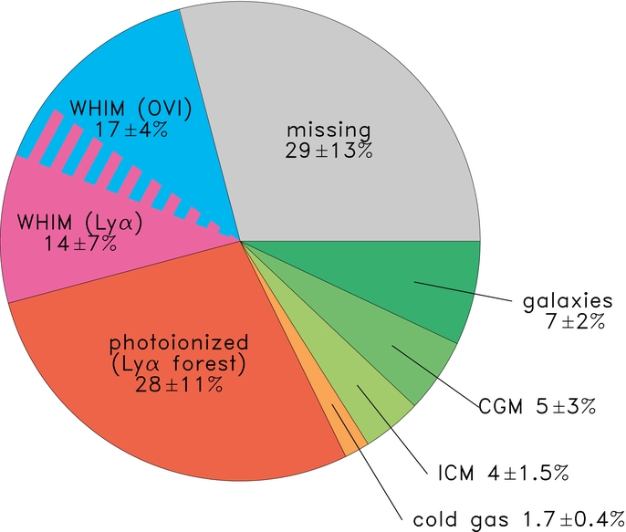
Figure 2: Pie chart of the baryon distribution in the local Universe (Shull et al.,, 2012). Significant amount of baryons ($\sim 30-40\%$) are still missing.

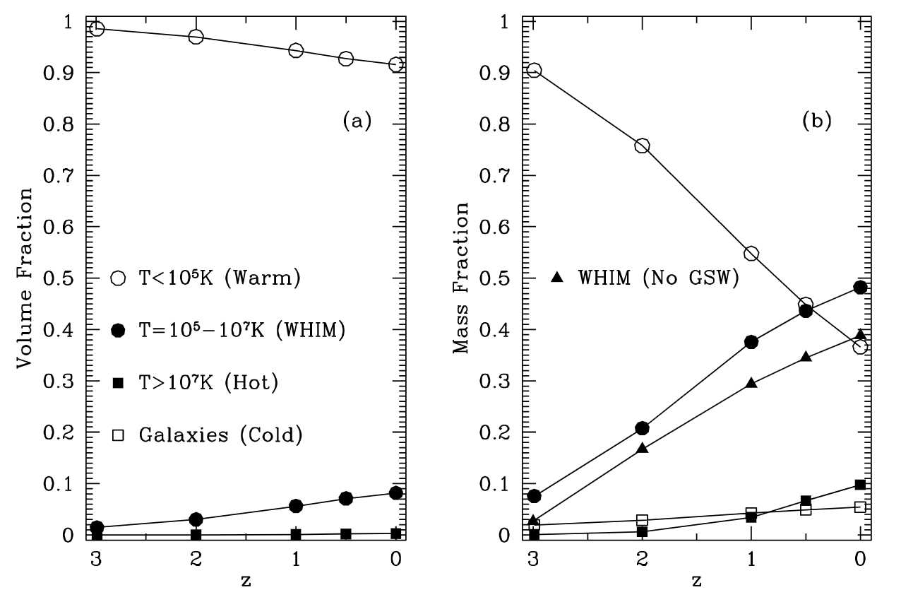
Figure 3: Redshift evolution of baryons at different temperatures (Cen and Ostriker,, 2006). Left (right) panel shows the evolution of volume (mass) fractions. At high redshift ($z\sim 3$), the vast majority of baryons ($>90$ %) are in cool gas probed by the Ly$\alpha$ forest. However, in local Universe, baryons in warm-hot phase ($10^{5}-10^{7}$ K, filled circles in both panels) become dominant. Triangles in the right panels represent WHIM in a cosmological simulation without feedbacks from galactic super-winds (GSWs).

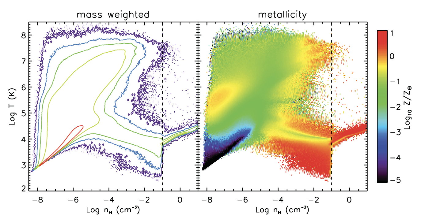
Figure 4: Mass-weighted baryon phase diagram (left panel), and metallicity distribution (right panel) from hydro-dynamical simulations (Bertone et al., 2013a, ).

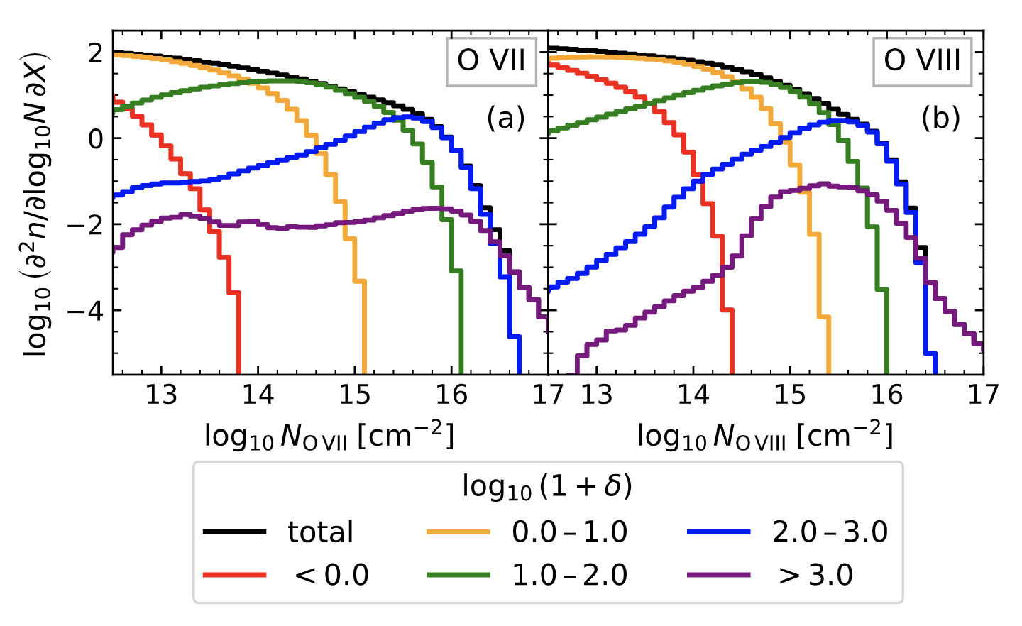
Figure 5: Column Density Distribution Functions (CDDFs) of O vii  (left panel) and O viii  (right panel) absorption line systems in simulations (Wijers et al.,, 2019). Lines with the highest column density are produced by absorption systems with the highest overdensities.

Figure 6: Baryonic mass vs. rotation velocity for systems from dwarfs galaxies to galaxy clusters (McGaugh et al.,, 2010). The solid line shows the baryonic mass of a system if it followed the cosmic universal baryon fraction (17%) of the dark matter mass.

2.2 The Large Scale Structure and the Warm-Hot Intergalactic Medium

In the current most-accepted cosmology model, structures of the Universe form hierarchically via gravitational collapse, with small structures forming earlier. This “concordance” model has been successfully proven by numerous observations in the past thirty years. Cosmological N-body plus hydro-dynamical simulations, based on this model, also predicted that while a fraction of baryons accretes to form collapsed structures, the majority of the matter in the Universe lies in the filaments and nodes of the cosmic-web form, and a significant amount may still reside in the intergalactic space (e.g., Cen and Ostriker,, 1999 and Figure 1).

Interestingly, the results from these numerical simulations provided a possible solution to the long-standing “missing baryons” problem. In the 1990s, a number of studies suggested a shortage of unaccounted baryons in the low-redshift Universe (e.g., Persic and Salucci,, 1992; Bristow and Phillipps,, 1994; Fukugita et al.,, 1998), by simply comparing the census of observed baryons in the local Universe with that indirectly derived from observations of the early Universe, i.e. the comparison of primordial deuterium abundance with big bang nucleosynthesis (BBN) models and the fluctuations of the CMB radiation.

Both, observations of the primordial deuterium abundance (Cooke et al.,, 2018) and the latest CMB measurements (Planck Collaboration et al.,, 2020), give a roughly consistent value of $\Omega_{b}\approx 0.045$, assuming a Hubble constant of $70\rm\ km\ s^{-1}Mpc^{-1}$. However, in the local Universe, counting all the baryons in the collapsed phases (galaxies, stars) and in the photoionized IGM (Ly$\alpha$ absorbers), one can detect at most 60% of the cosmic baryons predicted by BBN and CMB (Persic and Salucci,, 1992; Bristow and Phillipps,, 1994; Fukugita et al.,, 1998; Shull et al.,, 2012), leaving a shortfall of $\sim 40\%$, the so-called “missing baryons” (Figure 2).

Cosmological hydro-dynamical simulations provided the first hint of where to find these missing baryons (Hellsten et al.,, 1998; Cen and Ostriker,, 1999; Davé et al.,, 2001; Fang et al., 2002b, ; Chen et al.,, 2003; Cen and Ostriker,, 2006; Cen and Fang,, 2006; Branchini et al.,, 2009; Wijers et al.,, 2019). Figure 3 shows the volume (left panel) and mass (right panel) evolution of baryons as a function of redshift, for baryons at different temperature. At high redshift, the vast majority of the baryons (more than 90%) are located in the IGM in the form of warm-cool ($T<10^{5}\ K$), diffuse gas. However, at low redshift, the gas in the temperature range of $10^{5}-10^{7}\ K$ dominates with a mass fraction of 40 – 50%. This diffuse gas ($n_{b}=10^{-6}-10^{-4}$ cm^-3 or over-densities $\delta=n/<n>=n/[2\times 10^{-7}(1+z)^{3}(\Omega_{b}h^{2}/0.02)]=5-500$) permeates the intergalactic space in the LLS and forms the so-called “warm-hot intergalactic medium,” or WHIM (Cen and Ostriker,, 1999; Davé et al.,, 2001).

It is suggested that while initially the gas in the high-redshift IGM remains mainly photo-ionized by the meta-galactic radiation field at temperatures below $10^{5}\ K$, the subsequent collapse of material towards dark-mater potential wells that feeds the formation of structures, triggers shock waves along the filaments, and heats the gas in the IGM to temperatures in the range $10^{5}-10^{7}\ K$. Here we present a brief overview of theoretical predictions concerning the chemical and physical state of the WHIM and the potentials of X-ray absorption as a probe of its existence. A detailed discussion from the observational and detectability point of view, will be presented in section §3.

Metallicity: Metals, defined as elements heavier than hydrogen and helium, are important tracers of the WHIM. We still do not know precisely the metallicity of the diffused IGM, especially at low redshift, due to the lack of data. Numerical simulations suggest it could range between $10^{-4}$– $10^{-1}Z_{\odot}$, where $Z_{\odot}$ is the solar metallicity (see Figure 4 and Cen and Ostriker,, 2006; Oppenheimer and Davé,, 2008; Bertone et al., 2013b, ; Schaye et al.,, 2015). Metals in these simulations were typically produced via stellar processes such as Type II supernovae (SNe), Type Ia SNe and stellar mass loss in asymptotic giant branch stars, and then were transported out into the intergalactic space via galactic outflows powered by bursts of star formation and/or nuclear activity (Active Galactic Nuclei: AGNs). An important quantity, by an observational point of view, is the column density distribution of these metals, defined as their total number per unit area along a given line of sight. By comparing the column density distribution of metal species such as C iv and O vi , it is shown that the predictions from numerical simulations agree reasonably well with observations, although details may vary depending on factors such as the strengths of galactic winds and other sub-grid physics (e.g.,Cen and Ostriker,, 2006; Schaye et al.,, 2015).

Ionization: we know that both particle-collisions (during thermal shocks) and photo-ionization by the metagalactic ultraviolet background (UVB), must contribute to the ionization of the low-redshift IGM, by stripping its atoms of their electrons. The resulting ionized metals are generally named “H-like” (hydrogen-like), “He-like” (helium-like), “Li-like” (lithium-like), etc., to reflect the number of bound electrons they are left with (i.e. one, two, three, etc., respectively). In modeling the exact ionization state of the IGM (and thus in estimating the column density distribution of a specific ion), however, two important assumptions have not yet been vigorously tested due to the lack of data. First, to account for photo-ionization simulations assume a theoretical metagalactic ultraviolet backgroud (UVB) such as that proposed by Haardt and Madau, (2012); however, several studies suggested the Haardt & Madau UVB may underestimate the Hydrogen photoionization rates due to a low escape fraction of Lyman continuum photons (e.g., Kollmeier et al.,, 2014; Shull et al.,, 2015). Such uncertainty may impact the production of O vii and O viii at column densities lower than $\sim 10^{16}\rm\ cm^{-2}$ as they likely trace the low density gas that is predominately photo-ionized (Wijers et al.,, 2020). Second, when the recombination timescale is shorter than the ion-electron equilibration timescale, non-equilibrium ionization may impact the production of ions. However, due to the low density of the WHIM, the effect of non-equilibrium ionization is typically not significant (see, e.g., Kang et al.,, 2005; Yoshikawa and Sasaki,, 2006; Cen and Fang,, 2006; Oppenheimer et al.,, 2016; Wijers et al.,, 2020).

X-ray absorption: A useful quantity to describe the distribution of the predicted X-ray absorption line strengths, is the “X-ray Forest Distribution Function” (XFDF, Hellsten et al.,, 1998; Fang et al., 2002a, ), or equivalently “Column Density Distribution Function” (CDDF, Wijers et al.,, 2020):

$$f(N^{i},z)=\frac{\partial^{2}n}{\partial\log_{10}N^{i}\partial z}.$$ (1)

This function represents the number of absorption systems (for the ion species $i$) per unit log column density per unit redshift. Figure 5 (Wijers et al.,, 2020) shows the CDDF (or XFDF) distributions of O vii (left panel) and O viii (right panel). Colored curves represent contributions from gas in different density regions. Interestingly, a break point is present in both panels at around $10^{16}\rm\ cm^{-2}$, suggesting absorbers with higher column density may arise in the (rarer to blindly cross) high over-density, galactic halo regions (Wijers et al.,, 2020).

2.3 The Circumgalactic Medium

As noted in §1, a second “missing baryons” problem exists on galactic scale: The cold baryon fraction (cold gas + stars) in Milky-Way size galaxies is well-below the mean cosmic baryon fraction (see, e,g, McGaugh et al.,, 2010, and Figure 6). This “missing galactic baryons” problem is closely related to the “over-cooling” problem in the theory of galaxy formation and evolution (see, e.g., White and Rees,, 1978; Maller and Bullock,, 2004). In both semi-analytic and hydro-dynamical treatments of galaxy formation, hot gas cools to fuel ongoing star formation in Milky-Way-size galaxies. Standard treatments of cooling predict at least twice as much cold gas and stars in these galaxies as observed (see, e.g., Benson et al.,, 2003; Maller and Bullock,, 2004; Kereš et al.,, 2005). Moreover, even in these models with “over-cooling,” most of the baryons in galaxy halos larger than $10^{11.3}M_{\odot}$ remain in the hot phase.

Proposed solutions to the over-cooling problem often involve strong feedback from supernovae and AGN (e.g., Hernquist and Springel,, 2003), yet the impact that these prescriptions have on the surrounding gas remain largely untested. Another possibility is that the cooling itself is less efficient because the hot halos are more extended than previously suggested (Maller and Bullock,, 2004; Fukugita and Peebles,, 2006; Sommer-Larsen,, 2006). Regardless of the specific solution, a large fraction of the baryons that naively would have cooled onto galaxies, must either be seating around galaxies in quasi-stable extended hot halos, or have been blown out of galaxy halos all together. In principle, about half of the still missing baryons in the Universe (i.e. $\sim 15-20$% of the total baryons: see Fig. 2) could lie in the halos of galaxies (Fukugita and Peebles,, 2006; Sommer-Larsen,, 2006). When considered in this context, constraints on the hot gas distribution within galaxy halos provide an important test of galaxy formation theory and probes a fundamental issue in cosmology.

The theoretical development of this idea of extended hot halo is, not surprisingly, coincident with the rapid development of multi-wavelength observations of outskirts of galaxies at the interface between their stellar disks and the IGM. These observations clearly demonstrate that the circumgalactic medium, or CGM, may harbor substantial amount of baryons, and may play a vital roles in regulating galaxy formation and evolution (for reviews, see Bregman and Lloyd-Davies,, 2007; Putman et al.,, 2012; Tumlinson et al.,, 2017). Motivated by the latest observations, a number of analytic models were developed to explain multi-wavelength data (i.e., Maller and Bullock,, 2004; Faerman et al.,, 2017, 2020). These models typically assume that gas in the CGM is in hydrostatic equilibrium with the galaxy’s gravitational potential, and has a certain form of equation of state. After obtaining gas density and temperature profiles, these models can reasonably predict quantities such as absorbing column densities from Li- to H-like oxygen that are consistent with observations of our Milky Way. The CGM is discussed in detail in the Chapter “Probing the circumgalactic medium with X-ray absorption lines” of Section XI of this Handbook.

3 X-ray Techniques

3.1 Ionization Balance of the LSS gas in the Local Universe

As noted in §2, the WHIM (including its, relatively dense, CGM fraction) may account for 50-60% of the gas in the IGM, but as much as $\sim 30$% of the gas pervading the LSS at redshift $z$${{}_{<}\atop{}^{\sim}}$1 may be the residual photo-ionized Lyman-$\alpha$ Forest (Shull et al.,, 2012). Both the gas producing the Lyman-$\alpha$ Forest and the WHIM contain highly ionized gas pervading the space around and between the galaxies, but the mechanisms of ionization of these two important reservoirs of baryons and metals of the Universe are dramatically different. The gas in the Lyman-$\alpha$ Forest is purely photoionized by the meta-galactic radiation field (whose intensity depends on redshift), whereas the WHIM is mainly collisionally ionized through shocks during the collapse of density perturbation, but it also experiences the additional meta-galactic photoionization contribution, to a level that depends on its density. This yields to two different ionization structures: both phases contain highly ionized hydrogen and metals, but with different ion balances. Particularly, the Lyman-$\alpha$ Forest contains typically 1 neutral ion of hydrogen every $10^{3}-10^{4}$ atoms (Figure 7a, bottom panel), and is therefore able to imprint strong Lyman-$\alpha$ absorption in the far-ultraviolet (FUV) spectra of background quasars (e.g. Shull et al.,, 2012 and references therein), and the astrophysically most abundant metal (oxygen) is mainly between its C-like (i.e. with six bound electrons) and He-like (only two bound electrons) ions (Figure 7a, central panel). The WHIM, instead, contains only 1 neutral atom of H every $10^{6}-10^{7}$ atoms (Figure 7b, bottom panel), making it virtually transparent to FUV light, and oxygen is mainly distributed between its Li-like (three bound electrons) and fully-stripped ions (with the exception of a narrow range of temperatures at the lowest end of the WHIM temperature distribution, where C- through Be-like (four bound electrons) ions are relatively abundant: Figure 7b, central panel).

The different ionization structure of baryons and metals in the Lyman-$\alpha$ Forest and the WHIM is also shown in Figure 8, where the fractions of Li-like (O vi : blue) and H-like (O viii : red) ions of oxygen are plotted as a function of the fraction of its stable He-like ion (O vii ). Dashed lines are for gas in the Lyman-$\alpha$-Forest conditions, while continuous lines refer to WHIM conditions. As an example, in Figure 8, we highlight two regions (pink shaded circles) where each phase has Li- and H-like ions with similar fractional abundances but O vii  fractional abundances differing by a factor 2.5.

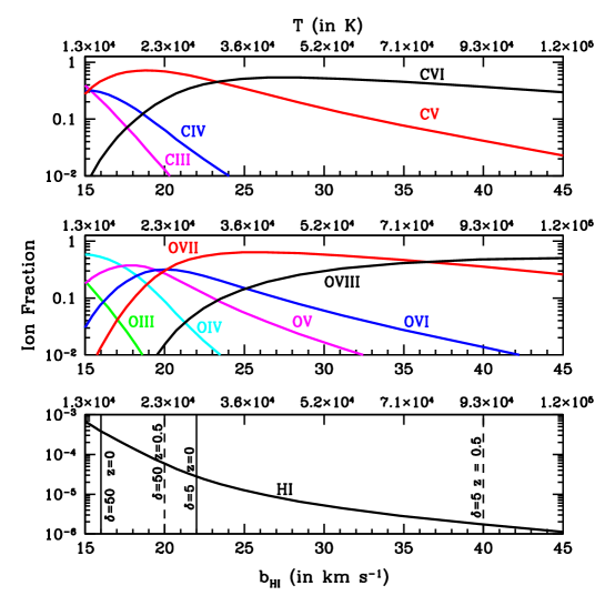
(a) Lyman-$\alpha$-Forest ionization balance

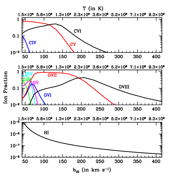
(b) WHIM ionization balance

Figure 7: Ionization balance of the most abundant ions of carbon (top panel), oxygen (central panel) and hydrogen (bottom panel), for (a) the Lyman-$\alpha$ Forest and (b) the WHIM, as a function of temperature (top x-axis) and HI Doppler parameter (bottom x-axis), i.e. the thermal width of hydrogen lines.

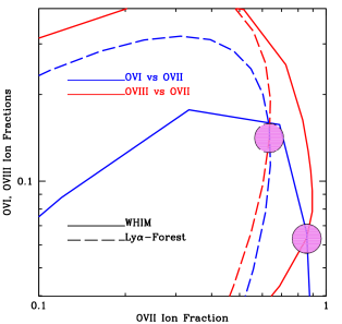
Figure 8: fractions of Li-like (blue lines) and H-like (red lines) ions of oxygen as a function of the fraction of the He-like ion of the same element, for purely photoionized Lyman-$\alpha$ Forest gas (dashed lines) and hybridly-ionized WHIM with density of $n_{e}=10^{-5}$ cm^-3 (i.e. over-density $\delta=50$; solid lines). The two phases have dramatically different ionization balances, as highlighted by, e.g., the two pink circles, where same relative amount of Li- and H-like ions of oxygen correspond to $2.5\times$ different amounts of O vii .

These differences in the ionization structures of the two main reservoirs of baryons in the low-redshift Universe, makes it relatively easy to observationally distinguish between them, provided that we have adequate quality spectra. In the following we concentrate on the optimal detection techniques of gas in the WHIM, in the soft X-ray band, bearing in mind that most of the arguments we use for the WHIM, and the same analysis techniques, apply to the low-$z$ photoionized Lyman-$\alpha$-Forest gas and that the two phases can be easily resolved through the above ionization-balance arguments.

3.2 The WHIM Absorption Observables

Because of the temperature and density intervals that define the WHIM, the bulk of this matter (with the important exception of the low-temperature tail of its distribution) is virtually transparent to FUV light, where the outer-shell (i.e. excitation of an electron from the most outermost shell of an ion) resonant transitions (i.e. electronic transitions allowed in the atomic dipole approximation) of neutral hydrogen, neutral and once-ionized helium and several relatively low ionization state and light metals, lie. This is not the case for the soft X-ray radiation, which is opaque to metal electronic transitions from virtually all ionization stages.

The soft X-ray band (namely E$\sim 0.2-3$ keV, or $\lambda\sim 4-120$ Å) contains thousands of inner- (excitation of an electron from an inner-shell to a still occupied outer-shell) and outer-shell resonant transitions and ionization edges from all metal ions (neutral through H-like) from C through Fe. Table 1 lists the strongest of these resonant transitions from the most abundant ions at WHIM physical conditions.

Table 1: Strongest Soft X-ray (0.3-3 keV) Resonant Transitions at WHIM physical Conditions

Element	Ion	aAbundance	Transition	Rest Frame	Rest Frame	bOscillator Strength	cInner/Outer
		relative to H		Energy	Wavelength
		(in $10^{-5}$)		(in eV)	(in Å)
Carbon	Li-like	$24$	$1s^{2}2s\rightarrow 1s2s2p$ (K$\alpha_{1}$)	d299.98	41.33	d0.483	I
Carbon	Li-like	$24$	$1s^{2}2s\rightarrow 1s2s2p$ (K$\alpha_{2}$)	d303.44	40.86	d0.041	I
Carbon	Li-like	$24$	$1s^{2}2s\rightarrow 1s2s3p$ (K$\beta$)	d336.50	36.85	d0.041	I
Carbon	He-like	$24$	$1s^{2}\rightarrow 1s2p$ (He$\alpha$)	e307.88	40.27	e0.648	O
Carbon	He-like	$24$	$1s^{2}\rightarrow 1s3p$ (He$\beta$)	e354.54	34.97	e0.141	O
Carbon	H-like	$24$	$1s\rightarrow 2p$ (Ly$\alpha$)	e367.47	33.74	e0.416	O
Carbon	H-like	$24$	$1s\rightarrow 3p$ (Ly$\beta$)	e435.49	28.47	e0.079	O
Nitrogen	Li-like	$7.95$	$1s^{2}2s\rightarrow 1s2s2p$ (K$\alpha_{1}$)	e421.47	29.42	f0.431	I
Nitrogen	Li-like	$7.95$	$1s^{2}2s\rightarrow 1s2s2p$ (K$\alpha_{2}$)	f425.45	29.21	f0.066	I
Nitrogen	He-like	$7.95$	$1s^{2}\rightarrow 1s2p$ (He$\alpha$)	e430.69	28.79	e0.675	O
Nitrogen	He-like	$7.95$	$1s^{2}\rightarrow 1s3p$ (He$\beta$)	e497.93	24.90	e0.144	O
Nitrogen	H-like	$7.95$	$1s\rightarrow 2p$ (Ly$\alpha$)	e500.34	24.78	e0.416	O
Nitrogen	H-like	$7.95$	$1s\rightarrow 3p$ (Ly$\beta$)	e592.93	20.91	e0.079	O
Oxygen	Li-like	$49$	$1s^{2}2s\rightarrow 1s2s2p$ (K$\alpha_{1}$)	g562.94	22.02	g0.328	I
Oxygen	Li-like	$49$	$1s^{2}2s\rightarrow 1s2s2p$ (K$\alpha_{2}$)	g567.62	21.84	g0.067	I
Oxygen	He-like	$49$	$1s^{2}\rightarrow 1s2p$ (He$\alpha$)	e573.95	21.60	e0.696	O
Oxygen	He-like	$49$	$1s^{2}\rightarrow 1s3p$ (He$\beta$)	e665.55	24.90	e0.146	O
Oxygen	H-like	$49$	$1s\rightarrow 2p$ (Ly$\alpha$)	e653.62	18.97	e0.416	O
Oxygen	H-like	$49$	$1s\rightarrow 3p$ (Ly$\beta$)	e774.61	16.01	e0.079	O
Neon	He-like	$8.7$	$1s^{2}\rightarrow 1s2p$ (He$\alpha$)	e922.01	13.45	e0.724	O
Neon	He-like	$8.7$	$1s^{2}\rightarrow 1s3p$ (He$\beta$)	e1073.77	11.55	e0.149	O
Neon	H-like	$8.7$	$1s\rightarrow 2p$ (Ly$\alpha$)	e1019.33	12.13	e0.416	O
Neon	H-like	$8.7$	$1s\rightarrow 3p$ (Ly$\beta$)	e1210.91	10.24	e0.079	O
Magnesium	He-like	$2.5$	$1s^{2}\rightarrow 1s2p$ (He$\alpha$)	e1352.24	9.17	e0.742	O
Magnesium	He-like	$2.5$	$1s^{2}\rightarrow 1s3p$ (He$\beta$)	e1579.31	7.85	e0.151	O
Magnesium	H-like	$2.5$	$1s\rightarrow 2p$ (Ly$\alpha$)	e1472.32	8.42	e0.416	O
Magnesium	H-like	$2.5$	$1s\rightarrow 3p$ (Ly$\beta$)	e1744.73	7.11	e0.079	O
Silicon	He-like	$1.9$	$1s^{2}\rightarrow 1s2p$ (He$\alpha$)	e1864.98	6.65	e0.757	O
Silicon	He-like	$1.9$	$1s^{2}\rightarrow 1s3p$ (He$\beta$)	e2182.55	5.68	e0.152	O
Silicon	H-like	$1.9$	$1s\rightarrow 2p$ (Ly$\alpha$)	e1995.79	6.18	e0.416	O
Silicon	H-like	$1.9$	$1s\rightarrow 3p$ (Ly$\beta$)	e2376.45	5.22	e0.079	O
Sulphur	He-like	$1.2$	$1s^{2}\rightarrow 1s2p$ (He$\alpha$)	e2460.63	5.04	e0.767	O
Sulphur	He-like	$1.2$	$1s^{2}\rightarrow 1s3p$ (He$\beta$)	e2883.35	4.30	e0.153	O
Sulphur	H-like	$1.2$	$1s\rightarrow 2p$ (Ly$\alpha$)	e2621.23	4.73	e0.416	O
Sulphur	H-like	$1.2$	$1s\rightarrow 3p$ (Ly$\beta$)	e3107.37	3.99	e0.079	O
Iron	Ne-like	$2.7$	$1s^{2}2s^{2}2p^{6}\rightarrow 1s^{2}s^{2}2p^{5}3d$ (L$\alpha$)	e825.73	15.02	e1.95	O

a. Wilms et al., (2000).
b. Absorption oscillator strength of the transition, defined by the relation $\mu_{lu}=A_{ul}\frac{g_{u}}{g_{l}}\frac{m_{e}c\lambda_{ul}^{2}}{8\pi^{2}e^{2}}$, where $A_{ul}$ is the rate of spontaneous-emission from the upper ($u$) to the lower ($l$ levels of the transition (Einstein coefficient $A$), $g_{l}$ and $g_{u}$ are the statistical weights of the lower and upper levels of the transition, respectively, and $\lambda_{ul}$ is the rest-frame wavelength of the transition.
c. Inner- (I) or Outer-shell (O) transition (see text for details).
d. Experiment: Müller et al., (2009).
e. Theory: Verner et al., (1996).
f. Experiment: Shorman et al., (2013).
g. Experiment: McLaughlin et al., (2017).

When the soft X-ray light from a background source (e.g. a quasar) intercepts chemically enriched gas along the line of sight, metals in the gas undergo resonant scattering by absorbing those line-of-sight photons with wavelengths $\lambda$ equal to their resonant transitions wavelengths, and re-emitting them randomly in all directions (on timescales given by the inverse of their Einstein coefficients for spontaneous emission, proportional to the transition oscillator strength: see, footnote ^b of Tab. 1 for definitions of these two quantities and, e.g., Rybicki and Lightman,, 1985 for details). The net effect is to take away those photons from our line of sight, and thus produce an absorption line in the spectrum of the background source.

For a given ion $i$ of the chemical element $X$ undergoing a $l\rightarrow u$ electronic transition, the two quantities directly observable/measurable are the strength of the line relative to the continuum (or equivalent width, $EW$) and the absorption line profile $\phi(\lambda)$. The two quantities are, generally, not independent of each other.

The line $EW$ is given by the ratio between the integrated line flux (assumed to be positive for absorption lines: lined areas in Figure 9a,b) and the monochromatic continuum flux at the line center normalized to 1 (see Figure 9a,b).

The absorption line profile is a combination of Gaussian and Lorentzian. The Gaussian broadening is due to thermal and non-thermal motions in the gas. The thermal, Doppler parameter of a line imprinted by the ion $X^{i}$, is given by:

$$b_{X^{i}}^{th}(T)=(2kT/m_{A})^{1/2}=(2kT/Am_{p})^{1/2}=b_{HI}^{th}(T)/A^{1/2},$$ (2)

where A is the atomic weight of the ion, $m_{p}$ is the proton mass and $b_{HI}^{th}(T)$ is the thermal Doppler parameter for hydrogen. The non-thermal motions could be due to turbulence or line-of-sight differential (e.g. the Hubble flow, for line-of-sight extended filaments) motions $\Delta\textrm{v}$. These two mechanisms combine together in quadrature to provide an effective Doppler parameter:

$$b=\sqrt{[b_{X^{i}}^{th}(T)]^{2}+(\Delta\textrm{v})^{2}}.$$ (3)

The Lorentzian broadening $\gamma$ is an intrinsic atomic feature of the given electronic transition and is implied by the uncertainty principle, due to the finite (non-zero) duration of an excited electronic state. The natural width of a transition $\gamma$ is proportional to the rate of decay of the upper level of the transition (into all possible lower-energy channels), i.e. to the oscillator strength $\mu_{lu}$ of the transition. These two distributions combine to provide a so called ’Voigt’ line profile (i.e. the average of the intrinsic Lorentzian line profile weighted by the Maxwellian particle velocity distribution: see e.g. Rybicki and Lightman,, 1985, for a full treatise). The ratio between the Lorentzian and Gaussian widths, defined as parameter $a$, determines the degree of saturation of a given line, and thus relates the two observables (line profile and Equivalent Widths).

Figure 9a,b show nine O vii _He-α and O vii _He-β absorption line profiles imprinted by an O vii  column density N${}_{OVII}=1.6\times 10^{15}$ cm^-2, in gas with temperatures ranging from T$=10^{5}-10^{7}$ K (oxygen thermal Doppler parameter $b_{O}=10-100$ km s^-1) and absence of turbulence or line-of-sight differential motion ($\Delta\textrm{v}=0$). The corresponding $a$ parameters of these two transitions range in the intervals $0.0056-0.056$ (Figure 9a) and $0.0014-0.014$ (Figure 9b), respectively. The He-$\alpha$ transition is intrinsically 4.8 times stronger than the He-$\beta$ (Table 1). This translates into shallower and broader (Gaussian dominated) He-$\beta$ lines, compared to He-$\alpha$.

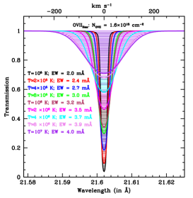
(a) O vii He-$\alpha$ line profiles

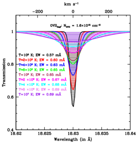
(b) O vii He-$\beta$ line profiles

Figure 9: Nine O vii _He-α (left panel (a)) and O vii _He-β (right panel (b)) absorption line profiles imprinted by gas with O vii  column density N${}_{OVII}=1.6\times 10^{15}$ cm^-2, and temperatures ranging from T$=10^{5}-10^{7}$ K ($b_{O}=10-100$ km s^-1). The non-thermal line broadening is assumed to be zero.

The absorption line profiles of Figure 9a,b are displayed at a spectral resolution of 0.2 mÅ (resolving powers $R=\lambda/\Delta\lambda\simeq 100,000$ at soft-X-ray wavelengths, corresponding to velocity resolutions of $\sim 3$ km s^-1, oversampling WHIM oxygen-line widths by factors ${{}_{>}\atop{}^{-}}$15) and infinite signal-to-noise per resolution element (SNRE). In these ideal conditions, line profiles and $EW$s can be directly and independently measured and thus ion column densities directly derived from single-line measurements.

Observationally, however, the situation is more complicated. Not only infinite SNRE is impossible to be attained, but the resolutions of the current (and future) generation of X-ray spectrometers are at least 100 times worse than those used in Figure 9 (see Table 2 in §5). The intrinsic degeneracy between line profiles and $EW$s is hidden into unresolved absorption line spectra, but can be removed by resorting to curve-of-growth techniques, applied to at least two different transitions from the same ion.

3.3 Absorption Line Curves of Growth

The curve of growth of an absorption line is the growth of line $EW$ with increasing ion column density and, as shown in Figure 9a,b, depends on the intrinsic strength of the transition and the physics and kinematics of the absorbing gas. Figures 10a,b, show the curves of growth of the two transitions of Figure 9a,b, respectively, for oxygen Doppler widths in the range $b_{O}=10-100$ km s^-1 (and no turbulence or line-of-sight differential motion: $\Delta\textrm{v}=0$).

At low ion column densities (below a threshold that depends on the intrinsic strength of the transition, namely its oscillator strength), $EW$s grow linearly with the number of line-of-sight particles. In this portion of the curve of growth, line $EW$s are independent on the line profile, and can be analytically approximated by eq. 4:

$$EW\simeq 8.85\times 10^{-18}\textrm{N}_{X^{i}}\lambda_{0}^{2}\mu_{X^{i}}\textrm{ m}\AA,$$ (4)

where N${}_{X^{i}}$ is the column density of the ion $i$ of the element $X$ in cm^-2, $\lambda_{0}$ is the central wavelength of the transition in Å and $\mu_{X^{i}}$ its oscillator strength. Above the column density threshold, absorption lines start saturating and their curves of growth bend into a non-linear regime, whose precise path in the $EW$-N${}_{X^{i}}$ plane depends critically on the line profile (and thus width).

The non-linear growth of absorption line $EW$s continues till a second (much higher and visible in Figure 10 only for the lowest temperature/thermal-broadening curves of growth) column density threshold, above which lines fully saturate to the zero-flux level and their $EW$s start increasing again with the square root of the ion column density (see (Spitzer,, 1978) for details).

In the saturated regimes, the $b-$N${}_{X^{i}}$ degeneracy can be removed by measuring the $EW$ of two transitions of the same ion. As an example, the shaded areas of Figure 10 show the range of allowed $EW$s of the O vii  $He-\alpha$ and $He-\beta$ transitions, corresponding to an O vii  column density N${}_{OVII}=4\times 10^{15}$ cm^-2. Determining, with sufficient accuracy, the $EW$s of the two transitions, allows one to find the unique $b-$N${}_{X^{i}}$ solution (see, e.g. Figure 11).

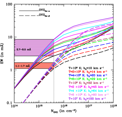
Figure 10: Curves of growth of the two transitions of Figure 9a,b (solid and dashed curves, respectively), for oxygen Doppler widths in the range $b_{O}=10-100$ km s^-1 (as labeled) and no turbulence or line-of-sight differential motion (i.e. $\Delta\textrm{v}=0$). The two shaded areas show the ranges of allowed $EW$s of the O vii  $He-\alpha$ (violet area) and $He-\beta$ (orange area) transitions, corresponding to an O vii  column density N${}_{OVII}=4\times 10^{15}$ cm^-2.

Figure 11: 90% O vii _He-α (black lines) and O vii _He-α (blue lines) $b-log(N_{\rm OVII})$ contours for measured $EW(He-\alpha)=5.4\pm 0.3$ mÅ and $EW(He-\beta)=1.5\pm 0.3$ mÅ. The green point and error bars show the best solution, while the magenta contours show the 90% solution for 2-interesting parameters.

3.4 WHIM Gas Diagnostics

With ion column densities and line widths in hands, the gas physical (e.g. ionization balance, and thus temperature, density, mass), kinematic (e.g. bulk and turbulent motion) and chemical (relative abundances) conditions can be derived.

WHIM Physical Conditions

The column density of the ion $i$ of the element $X$ is given by the product between the baryon equivalent column density N_b, the fractional abundance of the ion $i$ relatively to all ions of its element, $f_{X^{i}}$, and the chemical abundance of the element $A(X)$:

$$\textrm{N}_{X^{i}}=\textrm{N}_{b}f_{X^{i}}A(X).$$ (5)

Thus, the ratio of different ion column densities from different ions of the same element allow us to determine the gas ionization balance $\xi(f)$ = ($f_{X^{i}}/f_{X^{j}})$ (for $i\neq j$ and all elements $X$), and thus the physical state of the intervening gas and the mechanisms of ionization (pure collisions, pure photo-ionization or an hybrid combination of the two).

In the case of photo- or hybrid-ionization the source of photo-ionization are photons from the meta-galactic radiation field, which is relatively well known at $z$${{}_{<}\atop{}^{\sim}}$2 (e.g. Shull et al.,, 1999; Haardt and Madau,, 2012; but see §2.2 for possible sources of uncertainties). Thus, by modeling the measured gas ionization balance $\xi(f)$ with proper photo- or hybrid-ionization models, the density (or ionization parameter) and temperature of the gas can be estimated (see e.g. bottom panel of Figure 7a). For purely collisionally ionized gas (over-densities $\delta$ ${{}_{>}\atop{}^{\sim}}$500), the temperature of the gas is uniquely determined by the measured fractional ion abundances distribution $\xi(f)$.

WHIM Kinematics

The bulk line-of-sight velocities of the absorbing gas (or gas components, where multiple phases co-exist in the same structure) relative to, e.g., the redshift of the nearest galaxy, can be directly estimated by measuring the absorption line centroids, down to precisions that depend both on the spectrometer resolution and the S/N ratio at the line negative peaks. Velocity differences between different components of the same structure will inform us on the relative motions between physically different phases, e.g. the motion of warm (or even cold) condensations embedded in hotter and less dense filaments.

The widths of the absorption lines (or line components), instead, can in principle tell us about the ion kinetic temperature of the gas and line-of-sight turbulence or differential motions. As shown in §3.3 the width of the line $b$ contains two Gaussian broadening terms, caused by the thermal $b_{X^{i}}^{th}$ and turbulence (or line-of-sight differential) $\Delta\textrm{v}$ particle motion. For the generic ion $i$ of the elements $X$, we can write:

$$b_{X^{i}}=\sqrt{[b_{X^{i}}^{th}(T)]^{2}+(\Delta\textrm{v})^{2}}=\sqrt{[2kT/(A(X)m_{p})]+(\Delta\textrm{v})^{2}},$$ (6)

The thermal Doppler parameter depends on the atomic mass of the element imprinting the absorption line, while $\Delta\textrm{v}$ is the same for any ion. Thus with sufficiently high spectral resolution, by accurately measuring $b$ for at least two absorption lines from different elements $X$ and $Y$ (with $A(Y)>A(X)$), the two contributions can be resolved, and both the temperature of the gas and the line-of-sight turbulent motion directly estimated:

$$T=\frac{m_{p}}{2k}\frac{A(Y)A(X)}{A(Y)-A(X)}(b_{X^{i}}^{2}-b_{Y^{j}}^{2})=\frac{m_{p}}{2k}\frac{A(Y)A(X)}{A(Y)-A(X)}[(b_{X^{i}}^{th})^{2}-(b_{Y^{j}}^{th})^{2}].$$ (7)

$$(\Delta\textrm{v})^{2}=b_{X^{i}}^{2}-[b_{X^{i}}^{th}(T)]^{2}.$$ (8)

The directly measurable quantities $b_{X^{i}}$ and $b_{Y^{j}}$, however, differ generally by amounts that are at least one order of magnitude smaller than the resolution of the current (and most of the currently foreseen) X-ray spectrometers (see Table 2), even for $\Delta\textrm{v}=0$ (i.e. $b_{X^{i}}-b_{Y^{j}}=b_{X^{i}}^{th}-b_{Y^{j}}^{th}$) and for the largest possible difference in atomic weight. For example, for two absorption lines from carbon ($A(O)=12)$) and iron ($A(Fe)=52$) imprinted by gas at T$=10^{6}$ K, $b_{X^{i}}^{th}-b_{Y^{j}}^{th}\simeq 14$ km s^-1.

Practically, thus, until X-ray spectrometers with spectral resolution better than a few tens to hundred km s^-1 will be available (e.g. the XGS of Lynx, see Table 2), one has to rely on ionization-balance estimate and modelling (§3.4), to indirectly derive the temperature of the gas.

WHIM Chemical Conditions

Finally, knowing the physical conditions of the gas (i.e. the ionization balance distribution $\xi(f)$), one can estimate the relative abundances of the metals by their column density ratios. From Eq. 5:

$$\frac{A(Y)}{A(X)}=\frac{N_{Y^{j}}}{N_{X^{i}}}\frac{f_{X^{i}}}{f_{Y^{j}}}.$$ (9)

These can then be compared to relative metallicity yields observed in different astrophysical environments and at different redshifts, to gain insights on the sources of metal pollution of the WHIM and the evolution of WHIM/CGM metallicity with cosmic time, or with the relative metallicities of the nearest galaxy to obtain hints on the galaxy-CGM/IGM feedback mechanisms.

3.5 Feasibility of LSS gas absorption Observations

Detecting X-ray absorption lines from gas in the LSSs, requires X-ray spectrometers with high resolution and throughput.

Baryon densities in the range $n_{b}=10^{-6}-10^{-4}$ cm^-3 (over-densities $\delta\simeq 5-500$) and typical line of sight clouds (ranging from a fraction of galaxy’s CGM - depending on the line-of-sight-to-galaxy impact parameter - to that of an entire WHIM filament oriented along line of sight direction) with sizes between $0.1-1$ Mpc, imply expected baryon column density of the order of N${}_{b}\simeq 3\times(10^{17}-10^{19})$ cm^-2. For example, factoring a wide $Z=0.01-1Z_{\odot}$ range of metallicities, this yields, carbon, oxygen, neon and iron column densities N${}_{C}\simeq(10^{12}-10^{16})$ cm^-2, N${}_{O}\simeq 2\times(10^{12}-10^{16})$ cm^-2, N${}_{Ne}\simeq 2\times(10^{11}-10^{15})$ cm^-2and N${}_{Fe}\simeq(10^{11}-10^{15})$ cm^-2. The largest of these columns densities are expected from the densest WHIM environments, i.e. the nodes of the cosmic web, like outskirts of galaxy clusters or galaxy CGMs.

Eq. 4 allows us to derive loose upper limits (because of line saturation) to the rest-frame absorption line $EW$s expected from such ion column densities. He- and Ne-like ions are very stable both in purely photo-ionized or hybridly ionized gas, and their fractional abundance reaches values close to unity for wide ranges of ionization parameter or temperature (e.g. Figure 7). Assuming unity, then, for the ion fractional abundance, yields to maximum observed $EW$s of C, O and Ne $He-\alpha$ and Fe $Ne-L\alpha$ transitions: $EW($C v _He-α)$<30$ mÅ (0.2 eV), $EW($O vii _He-α)$<60$ mÅ (1.6 eV), $EW($Ne ix _He-α)$<10$ mÅ (0.7 eV) and $EW($Fe xvii _Ne-Lα)$<25$ mÅ (1.4 eV). Lower ion fractional abundance and/or metallicity, as well as line-saturation, further reduce these upper limits.

For a given absorption line with intrinsic width $b$ (in eV), the minimum $EW$ detectable in a spectrum with full-width-half-maximum resolution FWHM = $\Delta E$ (in eV) and signal to noise per resolution element $SNRE$ in the continuum, down to a single-line statistical significance N_σ and neglecting instrument systematics, is given by the following formula:

$$EW\geq\begin{cases}N_{\sigma}\frac{\sqrt{2.35b\Delta E}}{SNRE}\textrm{ eV},&\textrm{if}(2.35b)>\Delta E\textrm{ (resolved lines)}\\ &\\ N_{\sigma}\frac{\Delta E}{SNRE}\textrm{ eV},&\textrm{if}(2.35b)\leq\Delta E\textrm{ (unresolved lines)}\\ \end{cases}$$ (10)

Thus, a $\geq 5\sigma$ detection of, e.g., an unresolved 10 mÅ (0.2 eV at 0.5 keV) WHIM absorption line at 0.5 keV (close to the O vii He-$\alpha$ transition) in an X-ray spectrum with FWHM resolution $\Delta E$, requires $SNRE\geq 25\Delta E$ or, considering only Poisson noise, $\geq 625(\Delta E)^{2}$ counts per resolution elements.

The number of counts per resolution element depends on the brightness $F$ of the background source, the throughput $A_{eff}$ of the spectrometer and the exposure $T$ of the observation. Thus, under the Poisson-noise-only assumption (i.e. neglecting systematics and other possible sources of non-Poissonian errors), we can write:

$$SNRE=\sqrt{10^{-3}\times F_{E}\Delta EA_{eff}T_{\rm exp}},$$ (11)

or

$$\frac{T_{\rm exp}}{10^{3}}=\frac{SNRE^{2}}{F_{E}\Delta EA_{eff}}\textrm{ ks},$$ (12)

where $F_{E}$ is the specific photon flux at the energy $E$ in ph s^-1 cm^-2 keV^-1, $A_{eff}$ is the spectrometer effective area in cm², $\Delta E$ is the spectrometer resolution in eV and $T_{\rm exp}$ is the exposure time of the observation in s.

Let us consider a bright local Seyfert, with a 0.5-2 keV flux $F=2\times 10^{-11}$ erg cm^-2 s^-1 (1 mCrab). This, assuming for the 0.5-2 keV Seyfert spectrum a power-law with photon-index $\Gamma=2$ absorbed by a Galactic ISM column of $3\times 10^{20}$ cm^-2, translates into a 0.5 keV specific photon flux of $F_{E}\sim 0.032$ ph s^-1 cm^-2 keV^-1. Thus, from equations 10-12, the minimum exposure time required to detect an unresolved 0.5 keV absorption line with $EW=10$ mÅ (0.2 eV), against a 0.5-2 keV 1-mCrab background target and down to a single-line statistical significance of $\geq 5\sigma$, is

$$T_{\rm exp}\textrm{${{}_{>}\atop{}^{\sim}}${}}2\times 10^{4}\left(\frac{N_{\sigma}}{5}\right)^{2}\left(\frac{EW(eV)}{0.2}\right)^{-2}\left(\frac{F_{E}(ph\ s^{-1}cm^{-2}keV^{-1})}{0.032}\right)^{-1}\left(\frac{\Delta E(eV)}{A_{eff}(cm^{2})}\right)\textrm{ ks}.$$ (13)

The XMM-Newton Reflection Grating Spectrometer (RGS) has 0.5 keV spectral resolution $\Delta E=1.2$ eV and an effective area $A_{eff}(0.5keV)\simeq 40$ cm², yielding to large single-target exposures $T_{\rm exp}$${{}_{>}\atop{}^{\sim}}$600 ks. For the Chandra Low Energy Transmission Grating (LETG) spectrometer, with a slightly better spectral resolution ($\Delta E=1.0$ eV at 0.5 keV) but 4$\times$ lower effective area, $\sim$1 Ms exposures are required.

This is why the search for WHIM absorption lines with the currently available high-resolution X-ray spectrometers, has proven to be extremely challenging and only produced few (and controversial (e.g. Nicastro et al., 2005b ; Nicastro et al., 2005a ; Kaastra et al., 2006; Rasmussen et al., 2007; Fang et al., 2002b ; Cagnoni et al., 2004; Fang et al., 2007, 2010; Ren et al., 2014; Nicastro et al., 2016a ; Nicastro et al., 2018; Johnson et al., 2019) detections over the 20-year period started with the advent of the first 2 high-resolution X-ray spectrometers.

The situation will dramatically improve in the future (see §5). The Athena X-Ray Integral Field Unit (X-IFU), with its $\Delta E=2.5$ eV spectral resolution and 6,500 cm² effective area at 0.5 keV, will require only $T_{\rm exp}$${{}_{>}\atop{}^{\sim}}$7.5 ks observations to securely ($\geq 5\sigma$) detect the strongest ($\sim 10$ mÅ) WHIM lines against 1-mCrab targets. Much more common $EW=2-5$ mÅ (0.04-0.1 eV at 0.5 keV) WHIM lines will be detected against a 0.5-2 keV 1-mCrab target in $\sim 30-180$ ks and against 10 times fainter (and $\sim 100\times$ more numerous) targets, in $\sim 300-1800$ ks. This will open the route to the routine search and study of the diffuse gas in the LSS.

4 Observations

4.1 Currently available instruments

As seen in §3.5, intervening WHIM absorption lines are weak, requiring high spectral resolution in X-rays to detect them (§3). X-ray gratings became available with the launch of Chandra and XMM-Newton in 1999, opening a new window in the studies of the diffuse warm-hot gas. There are two types of gratings available on Chandra: Low Energy Transmission Grating (LETG) and High Energy Transmission Gratings (HETG). The HETG has two grating arms, a Medium Energy Grating and High Energy Grating. The LETG can be used with the ACIS-S detector or with the HRC-S detector (where ACIS is the Advanced CCD Imaging Spectrometer, HRC is the High Resolution Camera, and -S is for the spectroscopy mode). The XMM-Newton observatory has two Reflection Grating Spectrometers (RGS1 and RGS2). In Table 2 we provide the basic properties of these gratings.

4.2 Intervening X-ray absorption lines

With the newly deployed X-ray gratings on Chandra and XMM-Newton, astronomers could finally look for the missing baryons in the low-redshift WHIM. However, attempts to detect $z>0$ absorption lines were fraught with difficulties. While doing a blind search for intervening absorption lines, we have to pay a statistical penalty for chance fluctuations that may appear as lines. For example, HRC-LETG has 1,000 resolution elements in the $10$–$60$Å region. Therefore, there may be three ($(1-0.997)\times 1,000$) spurious “lines” in the spectrum with statistical significance of $>3\sigma$ (see e.g. Das et al.,, 2021). To counter this problem, often some redshift markers from ancillary observations (e.g. O vi absorbers in the UV) are used so that the location of the X-ray line is known a priory (Mathur et al.,, 2003).

In order to detect line-of-sight absorption lines, we need a bright background source. In the UV regime, bright quasars are used for this purpose. However, most quasars (particularly radio-quiet quasars), have intrinsic absorption lines. The high spectral resolution in the UV allows for easy separation of intrinsic absorption from the intervening absorption lines. This, however, becomes extremely difficult with current generation of X-ray grating spectroscopy. Therefore it is necessary to use blazars as background X-ray sources, as they have featureless continua.

With these considerations, efforts to detect the intervening X-ray absorption lines have been toward blazar sightlines (discussed below). Nevertheless, these have been largely unsuccessful, barring some notable exceptions. Even in the cases where the lines were reported, it was not clear whether they arise in the WHIM, or in the circumgalactic medium (CGM) of external galaxies, or in the intra-group medium. Below we discuss the efforts to detect the $z>0$ X-ray absorption lines as reported in literature.

Sightline to H 1821+642

A major effort to detect the WHIM with O vii absorption lines was made by Mathur et al., (2003) along the sightline to the blazar H 1821+642, using intervening O vi lines to select the absorber redshifts. Conclusive evidence for the WHIM detection was not reported by these authors, but their analysis provided ground work for future observations. They showed the power of using O vii, O viii lines in the X-ray band, together with the O vi line in the UV. In Figure 12, tracks of theoretical models are plotted in the $f$(O viii)$/f$(O vi) vs. $f$(O vii)$/f$(O vi) plane, where, e.g. $f$(O vii) is the ionization fraction of O vii. On the left, the tracks are for different gas overdensities, while on the right they are for different temperatures. We see that $f$(O vii)$/f$(O vi) is primarily a diagnostic of gas temperature, while $f$(O viii)$/f$(O vi) constrains the gas density for a given value of $f$(O vii)$/f$(O vi). This behavior reflects the competing roles of photoionization and collisional ionization, with the latter being more important for higher temperatures, higher densities, and lower ionization states (see also §3.2 and Fig. 8).

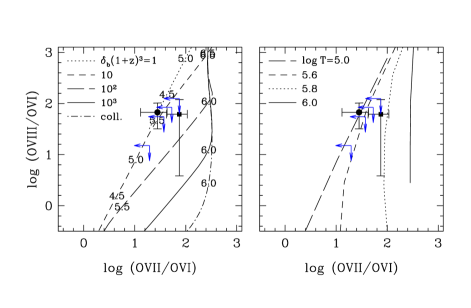
Figure 12: Constraints on the physical state of the intervening absorbers with O vi, O vii, and O viii : black points show the two tentative O vi-associated X-ray detections, while blue upper limits refer to the 4 O vi absorbers not detected in the X-rays. Left: Curves show the tracks in the $f$(O viii)$/f$(O vi) vs. $f$( O vii)$/f$(O vi) plane. Dotted, short-dashed, long-dashed, and solid lines are for gas overdensities $\delta_{b}(1+z)^{3}=1$, 10, $10^{2}$, and $10^{3}$, respectively, while the dot-dashed line represents pure collisional ionization. Numbers along these curves indicate $\log T$ in degrees Kelvin. Right: Same, but with tracks of constant temperature. Figure adapted from Mathur et al., (2003).

Kovács et al., (2019) stacked the Chandra spectrum around the wavelengths of the O vii lines at the redshifts of 17 intervening Lyman-$\alpha$ lines and detected the O vii line with $3.3\sigma$ significance. They found the O vii column density of $N_{\rm OVII}=1.4\pm 0.4\times 10^{15}$ cm^-2. Assuming that all the 17 systems contribute equally, they determined the gas density to be $n_{H}=1-2\times 10^{-6}$ cm^-3, corresponding to the density in the WHIM. However, theoretical simulations show that while O vi correlates with O vii and O viii in the WHIM, the same is not true for H i  (Wijers et al.,, 2019). Therefore it is unlikely that stacking on H i Lyman-$\alpha$ yields strong O vii absorption. Kovács et al., (2019) selected only those foreground Lyman-$\alpha$ absorbers that were associated with massive galaxies with $M_{\star}$${{}_{>}\atop{}^{\sim}}$$10^{10}$M_⊙, corresponding to $M_{\rm halo}$${{}_{>}\atop{}^{\sim}}$$3\times 10^{11}$M_⊙. It is therefore possible that the O vii absorption is dominated by the CGM of five of their galaxies with impact parameters within twice the virial radii.

Sightline to Mrk 421

Nicastro et al., 2005b reported detection of WHIM lines in the sightline to Mrk 421. In order to obtain a high SNRE spectrum, the authors monitored the blazars in the sky, and triggered Chandra observations when the source was about ten times brighter than the average. The resulting spectrum (Figure 13) led to the detection of two intervening systems at redshits $z=0.011\pm 0.001$ with the O vii K$\alpha$ absorption line and at $z=0.026\pm 0.001$ with N vii K$\alpha$ line.

Whether these systems are from the WHIM or from outskirts of galaxies is a matter of debate (Williams et al.,, 2010). Using the highest SNRE Chandra spectra, Das et al., (2021) did not detect the O vii absorption lines reported by Nicastro et al., 2005b (see Rasmussen et al., 2007 for non-detections in XMM-Newton data), but they did detect the O viii K$\alpha$ lines at the two redshifts, consistent with the upper limits in Nicastro et al., 2005b . Thus the detection and interpretation of the intervening absorption toward Mrk 421 remains inconclusive.

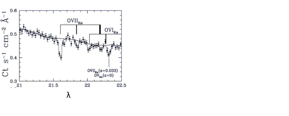
Figure 13: The Chandra spectrum towards Mrk 421 (from Nicastro et al., 2005b, ). Note the O vii K$\alpha$ lines at $z=0$ and at intervening redshifts of $z=0.011$ and $z=0.026$, marked with thin, thick, and very thick bars.

Sightline to PKS 2155-304

The first reported detection of the WHIM is along this sightline (Fang et al., 2002b, ). There are both O vi and broad Lyman-$\alpha$ intervening absorbers detected, providing good anchors for searching for X-ray lines. The most recent analysis of PKS 2155-304 spectra using Chandra and XMM-Newton is presented in Nevalainen et al., (2019), and the results are confusing. The deep XMM-Newton spectra did not result in the detetion of any absorption from the intervening systems. Chandra LETG/HRC spectra did not show any detected line either. However, the Chandra LETG/ACIS-S data yielded a line-like feature at $3.7\sigma$ which could be an O viii absorption line at the intervening redshift of $z=0.054$. The Chandra results are consistent with those reported previously (Fang et al., 2002b, ; Fang et al.,, 2007; Williams et al.,, 2007). While the detected line could be from the WHIM, the authors could not rule out that it could also be a transient feature associated with the blazar. Moreover, the detection itself is not robust given the inconsistency among different detectors.

Sightline to 3C 273

Absorption signatures along the sightline to this blazar were explored by Fang et al., (2003) using Chandra data. They reported on the detection of the O vii absorption line at $z=0$, but not from the intervening WHIM. Recently, Ahoranta et al., (2020) explored the same sightline with XMM-Newton and Chandra and reported the detection of O vii and Ne ix lines from the WHIM at $z=0.09017$ where a O vi system is detected in the UV. While they claim a $3.9\sigma$ combined significance of the detection, inspection of their spectra shows that the evidence is marginal. Moreover, as noted above in §4.2, there is a high probability of spurious lines with low statistical significance. Thus the presence of the WHIM detection in this sightline remains doubtful.

Sightlines to H 2356-309 and Mrk 501

The sightline to blazar H 2356-309 is interesting because it passes through the Sculptor Wall, a LSS of galaxies. The redshift of the LSS is known ($z\sim 0.03$), providing a marker for X-ray absorption lines. Chandra and XMM-Newton observations of this sightline were presented by Buote et al., (2009) who reported a $3\sigma$ detection of the O vii K$\alpha$ line. A deeper Chandra data yielded a $3.4\sigma$ line detection, and the significance increases to $4\sigma$ including the XMM-Newton data (Fang et al.,, 2010). A similar detection behind the Herculus wall ($z\sim 0.03$) in the sightline toward Mrk 501 was reported by Ren et al., (2014). However, both of these line detections from the putative WHIM (at the same redshift) were likely contaminated by O ii k$\beta$ lines from the interstellar medium of the Milky Way (Nicastro et al., 2016b, ).

Sightline to 1ES 1553+113

From the experience of observing several sightlines over the years, it was clear that deep observations of a blazar sightline are necessary to detect the WHIM with current generation of instruments. The sightline to 1ES1553+113 was observed with XMM-Newton for almost $1.8$Ms by Nicastro et al., (2018). The resulting spectrum reached SNRE$=33$ in the $23.5$–$30.2$Å spectral region (shown in Figure 14). The high SNRE allowed detections of weak absorption lines with $EW$${{}_{>}\atop{}^{-}}$$3.5$ mÅ. The authors reported the detections of two intervening absorption systems at $z1=0.4339$ and $z2=0.3551$. The $z1=0.4339$ system was detected with the X-ray lines of O vii K$\alpha$ and K$\beta$. The $z2=0.3551$ system was detected with the O vii K$\alpha$ X-ray line only. The existence of these systems was further corroborated by the presence of galaxy overdensities around the sightline at the absorber redshits. There is a broad H i Lyman-$\alpha$ absorber at the redshift of the $z1$ system. There are two H i Lyman-$\alpha$ absorbers close to the $z2$ system, though they are separated by $750$ km s^-1 .

However, Johnson et al., (2019) question whether the intervening absorption systems are truly from the WHIM. These authors present a deep redshift survey in the field of 1ES1553+113. They found that the blazar, whose spectroscopic redshift is still unknown, is likely a member of a group of galaxies, and that the $z1$ system arises in the intra-group medium. If the $z1$ system is associated with the LSS associated with the blazar, it should not be included in the statistics of the blind search. They also show that the $z2$ system arises in an isolated environment which they show to be unexpected for the WHIM. Therefore, Johnson et al., (2019) argue that the X-ray intervening systems do not trace the WHIM, and do not account for the missing low-redshift baryons (see §4.4).

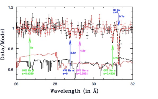
Figure 14: Left: The XMM-Newton spectrum towards 1ES1553+113 (from Nicastro et al.,, 2018) reporting the detections of the intervening absorption lines at $z1=0.4339$ and $z2=0.3551$. Shown are the normalized raw data (in bins with signal to noise per bin $\geq 30$) in RGS1 (black points and $1\sigma$ errorbars) and RGS2 (red points and $1\sigma$ errorbars). Thick dashed curves are RGS1 (black) and RGS2 (red) best-fitting model folded through the RGS response functions. Thin solid curves at the bottom of the graph are RGS1 (black) and RGS2 (red) effective areas (in arbitrary units), showing instrumental features due to cool-pixels in the detectors. Of the 5 absorption lines shown, only the weak O vii K$\beta$ at $z=0.4339$, and only in the RGS1, can be affected by the presence of an instrumental feature.

4.3 WHIM and the CGM

In the discussion above, we have been discussing the CGM alongside the WHIM. There are several reasons why it is difficult to distinguish between the WHIM and the CGM. Both are observed as intervening absorption systems, and unless we know of the presence of nearby galaxies, we cannot tell whether or not they arise within the CGM. Theoretical simulations do not necessarily distinguish between the two either. Both the WHIM and the CGM have $T\approx 10^{6}$K, and the gas is diffuse. The $T$–$n$ phase space in simulations, however, shows a wide range of densities at $T\approx 10^{6}$K (Figure 4) with denser gas belonging to the CGM while the truly diffuse gas (with density down to almost cosmological mean density) corresponding to the WHIM. However, with absorption lines we measure the column density, not the density, leading to the ambiguity in the inferences. New simulations are providing insights on linking density to column density. Using the EAGLE cosmological simulations, Wijers et al., (2019) studies the column density distribution functions (CDDF) of intervening O vii and O viii absorption systems (see §2.2). They found a break in the CDDF around the column density of $\rm\log N$(O vii)$=10^{16}cm^{-2}$ dominated by systems with overdensities of $\sim 100$. Therefore, absorption systems with column densities lower than the break likely arise in the diffuse portion of the WHIM, while those with higher column densities are from the CGM of collapsed halos (see Figure 15). The absorption systems detected so far (§4.2) are therefore likely from the CGM of external galaxies (or from the intra-group medium (§4.2)).

Another distinguishing characteristic between the dense (CGM) and the diffuse WHIM is the metallicity. The CGM is likely to be more metal-rich than the WHIM. Observationally it is difficult to measure the metallicity directly from X-ray observations alone. However, a combination of UV and X-ray spectroscopy would allow metallicity measurements and further distinguish the CGM and the WHIM. The CGM is discussed in detail in the Chapter “Probing the circumgalactic medium with X-ray absorption lines” of Section XI of this Handbook.

4.4 WHIM and the missing baryons

The intervening X-ray absorption lines from the WHIM allow us to determine the baryon content of the WHIM. Indeed, from the measured column density of the O vii ion one can obtain the baryon density of the low-redshift Universe as follows. Converting the O vii column density to the equivalent total column density depends on the temperature, oxygen abundance and metallicity of the WHIM. They are not directly measured with X-ray spectroscopy; therefore assumption are made, guided by theory (see §2). The next step is to convert the observed number density of the absorbers (number per unit redshift/pathlength) along a few sightlines to the cosmic baryon density. While this is an established method in the UV, we again need to resort to theoretical simulations in the X-ray band. This is because there are only a few sightlines with detections of intervening absorption, resulting in large errors on the number density of the absorbers. Secondly, the observations do not span the wide range of column densities to determine their distribution function empirically, so once again we need to resort to theoretical models. Additionally, the detected systems lie on the high end of the distribution function predicted by theoretical models (see Figure 15). As noted in §4.2 above, the lines may not be from the true WHIM, but from the CGM of nearby galaxies or from the intra-group medium, in which case they do not contribute to the column density distribution function of the WHIM. As such, there are many caveats in determining the observed baryon fraction in the WHIM from the X-ray detected gas.

Nevertheless, assuming that the two detected intervening absorption systems along the 1ES1553+113 sightlines are true detections, and that they are from the WHIM, and assuming that the extrapolation of the column density distribution function to lower columns is as predicted by theory, one can measure the cosmic baryon census (see Figure 16). According to Nicastro et al., (2018), the warm-hot gas traced by X-ray absorption lines can account for the missing baryons in the low-redshift Universe.

Figure 15: The distribution function of O vii EWs (from Wijers et al.,, 2019). The blue and cyan lines are from their EAGLE simulations; the dot-dashed lines are from the simulations of Cen and Fang, (2006); and the green dashed line is from Branchini et al., (2009). The two points with error-bars are from Nicastro et al., (2018).

Figure 16: Pie diagram of the baryonic components of the local Universe (from Nicastro et al.,, 2018).

5 Future

The future of LSS-absorption studies is bright. Several new X-ray missions (or mission concepts) have been studied and designed over the past 2 decades to overcome the limitations of current high-resolution X-ray spectrometers (namely, small effective area and relatively low spectral resolution: see §4.1 and 3.5) and some of these have been selected by space-agencies and are currently planned (or likely) to fly over the next two decades, such as Athena (Barcons et al.,, 2012), XRISM (Tashiro et al.,, 2018), Arcus (Smith,, 2020).

Modern, high-efficiency high-resolution X-ray spectrometers fall into two broad categories: dispersive and non-dispersive. In the following we schematically review the main properties, as well as advantages and disadvantages of these two types of spectrometers, for WHIM studies.

5.1 Dispersive Spectrometers

Dispersive X-ray spectrometers use X-ray gratings (see Section I of this book, Chapter Gratings for X-ray Astronomy) to diffract (in one dimension) photons onto an array of detectors with dispersion angles $\beta$ that depend linearly on the wavelength $\lambda$ of the incoming photons:

$$sin\beta=m\frac{\lambda}{p},$$ (14)

where the integer $m$ (0, 1, 2,…) is the order number and $p$ is the spatial period of the grating lines. Non-diffracted photons ($\beta=0$, or 0^th-order) form an image of the source on the detector, while higher-order photons are dispersed on the detector to a distance from the centroid of the 0^th-order image proportional to the order number and the energy of the photons. Thus, the energy resolution of gratings depends on the precision with which the photons are localized on the detectors (and so, in turn, on the spatial resolution of the mirror along the dispersion direction). Different orders, superimposed on the same dispersion axis, are separated by exploiting the (much lower) energy resolution of the detectors.

Because of the technique used to measure the energy of the incoming photons (eq. 14), the “natural” unit for grating spectrometers is the photon wavelength, in Å.

Currently operating grating spectrometers onboard Chandra  (Weisskopf,, 1999) are transmission gratings (i.e. interposed between the mirror and the focal plane, along the focal axis) while those onboard XMM-Newton  (Jansen et al.,, 2001) are reflection gratings (i.e. placed in the converging beam at the exit from the X-ray telescopes and reflecting photons to detectors offset from the telescope focal plane). These instruments have been designed several decades ago and are characterized by low diffraction efficiency (a few percent at 1 keV) and 1^st-order resolving powers of a few hundreds to a thousand over the covered spectral ranges (see Table 2).

New grating spectrometers with much improved efficiency (up to 60-70% at 1 keV: e.g. Heilmann et al.,, 2021) and constant resolving power over the covered energy band (obtained by exploiting different diffraction orders with enhanced intensity in different portions of the spectrum) of several thousands, have been developed over the past decade, and have reached high technical readiness levels (e.g. Heilmann et al.,, 2021; Smith,, 2020). These gratings have been proposed for several mission concepts (Table 2), e.g. WhimEx (Cash et al.,, 2011), Arcus (Smith,, 2020), Lynx (Gaskin et al.,, 2019), HiReX (Nicastro et al.,, 2021), and one of them (Arcus) was selected by NASA in 2016 for a phase-A concept study.

Dispersive spectrometers can reach today resolving powers $R$ of several thousands and up to R$\simeq 10,000$ and over (e.g. Günther and Heilmann,, 2019; Nicastro et al.,, 2021), thus approaching the resolution needed to directly measure the temperature of the absorbing gas by comparing line-widths imprinted by ions with different atomic weight (see §3.4). However, these types of high-resolution X-ray spectrometers allow only efficient spectroscopy of one target at a time (located in the proximity of the central region of the detector), and are optimally suited for point-like (i.e. non-spatially resolved) sources.

5.2 Non-Dispersive Spetrometers

To enable simultaneous spectroscopy of all (extended and point-like) sources present in the field of view (Integral-Field-Unit spectroscopy), arrays of non-dispersive high-resolution spectrometers (each representing a pixel of the detector) are needed in the focal plane of the mirror.

X-ray micro-calorimeters have been developed over the past two decades, and consist of essentially three elements: an absorber, a resistive thermometer and a heat-sink (or cooler).

The most developed X-ray micro-calorimeters are called Transition-Edge-Sensors (TESs: see Section II of this book, Chapter TES detectors (excluding fabrication) for details). The energy resolution of a TES is inversely proportional to the square root of a parameter $\alpha$ that measures the ability of a material to respond to temperature variations with changes in resistance, and can be written:

$$\Delta E\simeq 2.35\sqrt{4kT^{2}\frac{C}{\alpha}},$$ (15)

where $C$ is the TES’s heat capacity. Thus, the lower the operating temperature of the absorber and its heat-capacity, and the higher the parameter $\alpha$, the better the energy resolution. There are intrinsic limitations, however. TESs can only operate near their transition temperature $T_{c}$. At a given operating temperature, this implies a maximum $\Delta T$ in the TES, which in turn implies a maximum energy of the incoming photons:

$$E_{MAX}\simeq C\Delta T_{MAX}\simeq C\frac{T}{\alpha},$$ (16)

And finally, replacing Eq. 16 in 15, we get:

$$\Delta E\simeq 2.35\sqrt{4kTE_{MAX}},$$ (17)

Thus the resolution of a TES operating at 100 mK, cannot be better than $\simeq 1$ eV at 6 keV and $\simeq 0.4$ eV at 1 keV.

Several future (or planned) X-ray missions will have an array of TESs in their focal plane, e.g. XRISM (JAXA/NASA mission, planed launch-date year 2022; Tashiro et al.,, 2018) Athena (ESA large-mission, launch-date currently foreseen in year 2031; Barcons et al.,, 2012), Lynx (NASA mission concept, currently under decadal-review; Gaskin et al.,, 2019), HUBS (China National Space Administration - CNSA - mission concept, currently under study; Cui et al.,, 2020).

5.3 Detectability and Study of LSS Absorbers with Future Missions

As shown in Eq. 10 (§3), detecting absorption lines from gas in the LSS down to a given line EW requires large throughput and high-spectral resolution in the 0.2-2 keV band. We therefore define the square root of the product between the resolving power and the effective area of the detector at 0.5 keV, as a figure-of-merit for LSS absorption detectability (FoM_det). Table 2 summarizes the properties of the main, planned or under concept studies, future X-ray spectrometers and show their FoM_det, normalized to that of the current Chandra  HRC-LETG spectrometer.

Table 2: Current & Future high-resolution X-ray spectrometers

Mission	Spectrometer	Instrument	Effective Area	Resolving Power	Spectral Resolution	FoMdet Relative
			at 0.5 keV (in cm2)	at 0.5 keV	at 0.5 keV (in km s-1)	to Chandra LETG
Chandra	HRCS-LETG	Grating	c12	496	604	1
XMM-Newton	RGS1+RGS2	Grating	a40	382	785	1.6
XRISM	Resolve	TES	65	83	3612	0.95
Athena	X-IFU	TES	5900	200	1500	14.1
HUBS	XQSC	TES	450	$>$500	$<$600	$>$6.1
Arcus		Grating	800	2500	120	18.3
Lynx	XGS	Grating	$>4000$	$>5000$	$<$60	$>$58

a. First order

For each of these missions, systematic effects (uncalibrated pixel-to-pixel quantum efficiency variations) in the focal plane detector are the ultimate limit to the minimum detectable line equivalent width. For an assumed 3% systematic uncertainty, the minimum detectable equivalent width is 3% of the instrument resolution. Table 3 lists these minimum EWs (EW_min: Col. 4) for lines at 0.5 keV, together with the corresponding median column of O vii  K$\alpha$ (N${}_{OVII}^{min}$: Col. 5), as derived from EAGLE hydro-dynamical simulations (Figure 7 in Wijers et al.,, 2020). We also use Eq. 13 to derive the minimum exposure time (in Ms) needed to detect such LSS absorption lines at 0.5 keV down to the their systematic limit EW_min and against background-targets with 0.5-2 keV flux $f_{E}=1$ mCrab ($2\times 10^{-11}$ erg s^-1 cm^-2; Table 3, Col. 6). There are about 15 of such targets (AGNs, most of which blazars) in the extragalactic X-ray sky, covering a total line-of-sight redshift interval of $\Delta z=7.9$. In Table 3 (Cols 8 and 9), we therefore list also the total exposure (in yrs) needed to cover this redshift pathlength (Col. 7), together with the expected number of LSS absorbers per unit redshift down to the detectability limit N${}_{OVII}^{min}$ (Figure 5) and the total number of detectable LSS absorbers in the full $\Delta z=7.9$ pathlength. Finally, we define a second Figure of Merit for LSS absorber studies (FoM_std), given by the number of detectable 0.5 keV absorbers per year (ratio of Col. 10 to 9).

Table 3: Maximum Detectabillity of LSS absorbers with current and future Missions

Mission	Spectrometer	Instrument	EWmin	N${}_{OVII}^{min}$	Tmin	T${}_{min}\times 15$	Systems	Total Number	FoMstd
			at 0.5 keV (in eV)	(in $10^{15}$ cm-2)	(in Ms)	(in yrs)	per unit z	of Systems	(in yr-1)
Chandra	HRCS-LETG	Grating	0.03	0.5	27	13	15.8	125	10
XMM-Newton	RGS1+RGS2	Grating	0.04	0.7	5.9	2.9	12.6	100	34
XRISM	Resolve	TES	0.2	5.0	0.7	0.3	4	32	107
Athena	X-IFU	TES	0.075	1.6	0.02	0.026	10	79	3038
HUBS	XQSC	TES	$<$0.03	$<$0.5	$<$0.7	$<$0.3	$>$15.8	$>$125	$>$417
Arcus		Grating	0.006	0.1	2	1	40	316	316
Lynx	XGS	Grating	$<0.003$	$<0.05$	$<0.8$	$<0.4$	$>50$	$>395$	$>$988

Generally, dispersive spectrometers, with no intrinsic limitations on resolving power, score better than microcalorimeters in detectability-power (FoM_det: Table 2), and can perform LSS absorption studies down to lower ion column densities (Table 2, Col. 5). However, only missions that combine a large throughput with a high resolving power can guarantee high investigation-powers (FoM_sdt). Particularly the Athena observatory scores by far the highest in FoM_std. It will allow the study of about 3000 LSS absorbers in a full year of observations of bright targets down to a column density of O vii  N${}_{OVII}\simeq 1.6\times 10^{15}$ cm^-2. This will enable the systematic investigation of the physics, kinematics and chemistry of the most massive LSS gaseous structures, permeating halos of thousands $\geq$L^∗ galaxies with masses in the $10^{12}-10^{13.5}$ M_⊙ range (Wijers et al.,, 2020). The HUBS mission, should allow to take these studies down to three times smaller O vii  column densities, corresponding to halo masses of $\simeq 10^{11.5}$, while high resolving-power grating missions like Arcus and Lynx will extend these systematic studies down to the halos of 0.05L^∗ galaxies (e.g. Wijers et al.,, 2020), so uncovering the entire spectrum of gaseous baryons and metals in the LSS.

References

- Ahoranta et al., (2020) Ahoranta, J., Nevalainen, J., Wijers, N., Finoguenov, A., Bonamente, M., Tempel, E., Tilton, E., Schaye, J., Kaastra, J., and Gozaliasl, G. (2020). Hot WHIM counterparts of FUV O VI absorbers: Evidence in the line-of-sight towards quasar 3C 273. A&A, 634:A106.
- Aldcroft et al., (1994) Aldcroft, T., Elvis, M., McDowell, J., and Fiore, F. (1994). X-Ray Constraints on the Intergalactic Medium. ApJ, 437:584.
- Barcons et al., (2012) Barcons, X., Barret, D., Decourchelle, A., den Herder, J. W., Dotani, T., Fabian, A. C., Fraga-Encinas, R., Kunieda, H., Lumb, D., Matt, G., Nandra, K., Piro, L., Rando, N., Sciortino, S., Smith, R. K., Strüder, L., Watson, M. G., White, N. E., and Willingale, R. (2012). Athena (advanced telescope for high energy astrophysics) assessment study report for esa cosmic vision 2015-2025.
- Benson et al., (2003) Benson, A. J., Bower, R. G., Frenk, C. S., Lacey, C. G., Baugh, C. M., and Cole, S. (2003). What Shapes the Luminosity Function of Galaxies? ApJ, 599(1):38–49.
- (5) Bertone, S., Aguirre, A., and Schaye, J. (2013a). How the diffuse Universe cools. MNRAS, 430(4):3292–3313.
- (6) Bertone, S., Aguirre, A., and Schaye, J. (2013b). How the diffuse Universe cools. MNRAS, 430(4):3292–3313.
- Branchini et al., (2009) Branchini, E., Ursino, E., Corsi, A., Martizzi, D., Amati, L., den Herder, J. W., Galeazzi, M., Gendre, B., Kaastra, J., Moscardini, L., Nicastro, F., Ohashi, T., Paerels, F., Piro, L., Roncarelli, M., Takei, Y., and Viel, M. (2009). Studying the Warm Hot Intergalactic Medium with Gamma-Ray Bursts. ApJ, 697(1):328–344.
- Bregman and Lloyd-Davies, (2007) Bregman, J. N. and Lloyd-Davies, E. J. (2007). X-Ray Absorption from the Milky Way Halo and the Local Group. ApJ, 669(2):990–1002.
- Bristow and Phillipps, (1994) Bristow, P. D. and Phillipps, S. (1994). On the Baryon Content of the Universe. MNRAS, 267:13.
- Buote et al., (2009) Buote, D. A., Zappacosta, L., Fang, T., Humphrey, P. J., Gastaldello, F., and Tagliaferri, G. (2009). X-Ray Absorption by WHIM in the Sculptor Wall. ApJ, 695(2):1351–1356.
- Cagnoni et al., (2004) Cagnoni, I., Nicastro, F., Maraschi, L., Treves, A., and Tavecchio, F. (2004). A View of PKS 2155-304 with XMM-Newton Reflection Grating Spectrometers. ApJ, 603(2):449–455.
- Cash et al., (2011) Cash, W., Mcentaffer, R., Zhang, W., Casement, L., Lillie, C., Schattenburg, M., Bautz, M., Holland, A., Tsunemi, H., and O’Dell, S. (2011). X-ray optics for whimex: the warm hot intergalactic medium explorer. 8147.
- Cen and Fang, (2006) Cen, R. and Fang, T. (2006). Where Are the Baryons? III. Nonequilibrium Effects and Observables. ApJ, 650(2):573–591.
- Cen and Ostriker, (1999) Cen, R. and Ostriker, J. P. (1999). Where Are the Baryons? ApJ, 514(1):1–6.
- Cen and Ostriker, (2006) Cen, R. and Ostriker, J. P. (2006). Where Are the Baryons? II. Feedback Effects. ApJ, 650(2):560–572.
- Chen et al., (2003) Chen, X., Weinberg, D. H., Katz, N., and Davé, R. (2003). X-Ray Absorption by the Low-Redshift Intergalactic Medium: A Numerical Study of the Cold Dark Matter Model. ApJ, 594(1):42–62.
- Connor et al., (2018) Connor, T., Kelson, D. D., Mulchaey, J., Vikhlinin, A., Patel, S. G., Balogh, M. L., Joshi, G., Kraft, R., Nagai, D., and Starikova, S. (2018). Wide-field Optical Spectroscopy of Abell 133: A Search for Filaments Reported in X-Ray Observations. ApJ, 867(1):25.
- Connor et al., (2019) Connor, T., Zahedy, F. S., Chen, H.-W., Cooper, T. J., Mulchaey, J. S., and Vikhlinin, A. (2019). COS Observations of the Cosmic Web: A Search for the Cooler Components of a Hot, X-Ray Identified Filament. ApJL, 884(1):L20.
- Cooke et al., (2018) Cooke, R. J., Pettini, M., and Steidel, C. C. (2018). One Percent Determination of the Primordial Deuterium Abundance. ApJ, 855(2):102.
- Cui et al., (2020) Cui, W., Bregman, J. N., Bruijn, M. P., Chen, L.-B., Chen, Y., Cui, C., Fang, T.-T., Gao, B., Gao, H., Gao, J.-R., Gottardi, L., Gu, K.-X., Guo, F.-L., Guo, J., He, C.-L., He, P.-F., den Herder, J.-W., Huang, Q.-S., Li, F.-J., Li, J.-T., Li, J.-J., Li, L.-Y., Li, T.-P., Li, W.-B., Liang, J.-T., Liang, Y.-J., Liang, G.-Y., Liu, Y.-J., Liu, Z., Liu, Z.-Y., Jaeckel, F., Ji, L., Ji, W., Jin, H., Kang, X., Ma, Y.-X., McCammon, D., Mo, H.-J., Nagayoshi, K., Nelms, K., Qi, R., Quan, J., Ridder, M. L., Shen, Z.-X., Simionescu, A., Taralli, E., Wang, Q. D., Wang, G.-L., Wang, J.-J., Wang, K., Wang, L., Wang, S.-F., Wang, S.-J., Wang, T.-G., Wang, W., Wang, X.-Q., Wang, Y.-L., Wang, Y.-R., Wang, Z., Wang, Z.-S., Wen, N.-Y., de Wit, M., Wu, S.-F., Xu, D., Xu, D.-D., Xu, H.-G., Xu, X.-J., Xu, R.-X., Xue, Y.-Q., Yi, S.-Z., Yu, J., Yang, L.-W., Yuan, F., Zhang, S., Zhang, W., Zhang, Z., Zhong, Q., Zhou, Y., and Zhu, W.-X. (2020). HUBS: a dedicated hot circumgalactic medium explorer. In den Herder, J.-W. A., Nikzad, S., and Nakazawa, K., editors, Space Telescopes and Instrumentation 2020: Ultraviolet to Gamma Ray, volume 11444, pages 470 – 481. International Society for Optics and Photonics, SPIE.
- Das et al., (2021) Das, S., Mathur, S., Gupta, A., and Krongold, Y. (2021). The hot circumgalactic medium of the Milky Way: evidence for super-virial, virial, and sub-virial temperature, non-solar chemical composition, and non-thermal line broadening. arXiv e-prints, page arXiv:2106.13243.
- Davé et al., (2001) Davé, R., Cen, R., Ostriker, J. P., Bryan, G. L., Hernquist, L., Katz, N., Weinberg, D. H., Norman, M. L., and O’Shea, B. (2001). Baryons in the Warm-Hot Intergalactic Medium. ApJ, 552(2):473–483.
- Davis et al., (1982) Davis, M., Huchra, J., Latham, D. W., and Tonry, J. (1982). A survey of galaxy redshifts. II. The large scale space distribution. ApJ, 253:423–445.
- de Graaff et al., (2019) de Graaff, A., Cai, Y.-C., Heymans, C., and Peacock, J. A. (2019). Probing the missing baryons with the Sunyaev-Zel’dovich effect from filaments. A&A, 624:A48.
- Eckert et al., (2015) Eckert, D., Jauzac, M., Shan, H., Kneib, J.-P., Erben, T., Israel, H., Jullo, E., Klein, M., Massey, R., Richard, J., and Tchernin, C. (2015). Warm-hot baryons comprise 5-10 per cent of filaments in the cosmic web. Nature, 528(7580):105–107.
- Faerman et al., (2017) Faerman, Y., Sternberg, A., and McKee, C. F. (2017). Massive Warm/Hot Galaxy Coronae as Probed by UV/X-Ray Oxygen Absorption and Emission. I. Basic Model. ApJ, 835(1):52.
- Faerman et al., (2020) Faerman, Y., Sternberg, A., and McKee, C. F. (2020). Massive Warm/Hot Galaxy Coronae. II. Isentropic Model. ApJ, 893(1):82.
- (28) Fang, T., Bryan, G. L., and Canizares, C. R. (2002a). Simulating the X-Ray Forest. ApJ, 564(2):604–623.
- Fang et al., (2010) Fang, T., Buote, D. A., Humphrey, P. J., Canizares, C. R., Zappacosta, L., Maiolino, R., Tagliaferri, G., and Gastaldello, F. (2010). Confirmation of X-ray Absorption by Warm-Hot Intergalactic Medium in the Sculptor Wall. ApJ, 714(2):1715–1724.
- Fang and Canizares, (2000) Fang, T. and Canizares, C. R. (2000). Probing Cosmology with the X-Ray Forest. ApJ, 539(2):532–539.
- Fang et al., (2007) Fang, T., Canizares, C. R., and Yao, Y. (2007). Confirming the Detection of an Intergalactic X-Ray Absorber toward PKS 2155-304. ApJ, 670(2):992–999.
- (32) Fang, T., Marshall, H. L., Lee, J. C., Davis, D. S., and Canizares, C. R. (2002b). Chandra Detection of O VIII Ly Absorption from an Overdense Region in the Intergalactic Medium. ApJL, 572(2):L127–L130.
- Fang et al., (2003) Fang, T., Sembach, K. R., and Canizares, C. R. (2003). Chandra Detection of Local O VII He Absorption along the Sight Line toward 3C 273. ApJL, 586(1):L49–L52.
- Field, (1972) Field, G. B. (1972). Intergalactic Matter. ARA&A, 10:227.
- Fukugita et al., (1998) Fukugita, M., Hogan, C. J., and Peebles, P. J. E. (1998). The Cosmic Baryon Budget. ApJ, 503(2):518–530.
- Fukugita and Peebles, (2006) Fukugita, M. and Peebles, P. J. E. (2006). Massive Coronae of Galaxies. ApJ, 639(2):590–599.
- Gaskin et al., (2019) Gaskin, J. A., Swartz, D., Vikhlinin, A. A., Ãzel, F., Gelmis, K. E. E., Arenberg, J. W., Bandler, S. R., Bautz, M. W., Civitani, M. M., Dominguez, A., Eckart, M. E., Falcone, A. D., Figueroa-Feliciano, E., Freeman, M. D., GÃŒnther, H. M., Jr., K. A. H., Heilmann, R. K., Kilaru, K., Kraft, R. P., McCarley, K. S., McEntaffer, R. L., Pareschi, G., Purcell, W. R., Reid, P. B., Schattenburg, M. L., Schwartz, D. A., Sr., E. D. S., Tananbaum, H. D., Tremblay, G. R., Zhang, W. W., and Zuhone, J. A. (2019). Lynx X-Ray Observatory: an overview. Journal of Astronomical Telescopes, Instruments, and Systems, 5(2):1 – 15.
- Gunn and Peterson, (1965) Gunn, J. E. and Peterson, B. A. (1965). On the Density of Neutral Hydrogen in Intergalactic Space. ApJ, 142:1633–1636.
- Günther and Heilmann, (2019) Günther, H. M. and Heilmann, R. K. (2019). Design progress on the Lynx soft x-ray critical-angle transmission grating spectrometer. In UV, X-Ray, and Gamma-Ray Space Instrumentation for Astronomy XXI, volume 11118 of Society of Photo-Optical Instrumentation Engineers (SPIE) Conference Series, page 111181C.
- Gupta et al., (2012) Gupta, A., Mathur, S., Krongold, Y., Nicastro, F., and Galeazzi, M. (2012). A Huge Reservoir of Ionized Gas around the Milky Way: Accounting for the Missing Mass? ApJL, 756:L8.
- Haardt and Madau, (2012) Haardt, F. and Madau, P. (2012). RADIATIVE TRANSFER IN a CLUMPY UNIVERSE. IV. NEW SYNTHESIS MODELS OF THE COSMIC UV/x-RAY BACKGROUND. 746(2):125.
- Heilmann et al., (2021) Heilmann, R., Huenemoerder, D., and Schattenburg, M. (2021). The importance of general technology development: The example of the critical-angle transmission grating a white paper submitted to the discipline program panel on electromagnetic observations from space (eos) in response to the astro2010 call for white papers on technology development.
- Hellsten et al., (1998) Hellsten, U., Gnedin, N. Y., and Miralda-Escudé, J. (1998). The X-Ray Forest: A New Prediction of Hierarchical Structure Formation Models. ApJ, 509(1):56–61.
- Hernquist and Springel, (2003) Hernquist, L. and Springel, V. (2003). An analytical model for the history of cosmic star formation. MNRAS, 341(4):1253–1267.
- Jansen et al., (2001) Jansen, F., Lumb, D., Altieri, B., Clavel, J., Ehle, M., Erd, C., Gabriel, C., Guainazzi, M., Gondoin, P., Much, R., Munoz, R., Santos, M., Schartel, N., Texier, D., and Vacanti, G. (2001). XMM-Newton observatory. I. The spacecraft and operations. A&A, 365:L1–L6.
- Johnson et al., (2019) Johnson, S. D., Mulchaey, J. S., Chen, H.-W., Wijers, N. A., Connor, T., Muzahid, S., Schaye, J., Cen, R., Carlsten, S. G., Charlton, J., Drout, M. R., Goulding, A. D., Hansen, T. T., and Walth, G. L. (2019). The Physical Origins of the Identified and Still Missing Components of the Warm-Hot Intergalactic Medium: Insights from Deep Surveys in the Field of Blazar 1ES1553+113. ApJL, 884(2):L31.
- Kaastra et al., (2006) Kaastra, J. S., Werner, N., Herder, J. W. A. d., Paerels, F. B. S., de Plaa, J., Rasmussen, A. P., and de Vries, C. P. (2006). The O VII X-Ray Forest toward Markarian 421: Consistency between XMM-Newton and Chandra. ApJ, 652(1):189–197.
- Kang et al., (2005) Kang, H., Ryu, D., Cen, R., and Song, D. (2005). Shock-heated Gas in the Large-Scale Structure of the Universe. ApJ, 620(1):21–30.
- Kereš et al., (2005) Kereš, D., Katz, N., Weinberg, D. H., and Davé, R. (2005). How do galaxies get their gas? MNRAS, 363(1):2–28.
- Kollmeier et al., (2014) Kollmeier, J. A., Weinberg, D. H., Oppenheimer, B. D., Haardt, F., Katz, N., Davé, R., Fardal, M., Madau, P., Danforth, C., Ford, A. B., Peeples, M. S., and McEwen, J. (2014). The Photon Underproduction Crisis. ApJL, 789(2):L32.
- Kovács et al., (2019) Kovács, O. E., Bogdán, Á., Smith, R. K., Kraft, R. P., and Forman, W. R. (2019). Detection of the Missing Baryons toward the Sightline of H1821+643. ApJ, 872(1):83.
- Lee et al., (2021) Lee, K.-G., Ata, M., Khrykin, I. S., Huang, Y., Prochaska, J. X., Cooke, J., Zhang, J., and Batten, A. (2021). Constraining the Cosmic Baryon Distribution with Fast Radio Burst Foreground Mapping. arXiv e-prints, page arXiv:2109.00386.
- Macquart et al., (2020) Macquart, J. P., Prochaska, J. X., McQuinn, M., Bannister, K. W., Bhandari, S., Day, C. K., Deller, A. T., Ekers, R. D., James, C. W., Marnoch, L., Osłowski, S., Phillips, C., Ryder, S. D., Scott, D. R., Shannon, R. M., and Tejos, N. (2020). A census of baryons in the Universe from localized fast radio bursts. Nature, 581(7809):391–395.
- Maller and Bullock, (2004) Maller, A. H. and Bullock, J. S. (2004). Multiphase galaxy formation: high-velocity clouds and the missing baryon problem. MNRAS, 355(3):694–712.
- Mathur et al., (2003) Mathur, S., Weinberg, D. H., and Chen, X. (2003). Tracing the Warm-Hot Intergalactic Medium at Low Redshift: X-Ray Forest Observations toward H1821+643. ApJ, 582(1):82–94.
- McGaugh et al., (2010) McGaugh, S. S., Schombert, J. M., de Blok, W. J. G., and Zagursky, M. J. (2010). The Baryon Content of Cosmic Structures. ApJL, 708(1):L14–L17.
- McLaughlin et al., (2017) McLaughlin, B. M., Bizau, J. M., Cubaynes, D., Guilbaud, S., Douix, S., Shorman, M. M. A., Ghazaly, M. O. A. E., Sakho, I., and Gharaibeh, M. F. (2017). K-shell photoionization of O4+ and O5+ ions: experiment and theory. MNRAS, 465(4):4690–4702.
- McQuinn, (2014) McQuinn, M. (2014). Locating the “Missing” Baryons with Extragalactic Dispersion Measure Estimates. ApJL, 780(2):L33.
- McQuinn, (2016) McQuinn, M. (2016). The Evolution of the Intergalactic Medium. ARA&A, 54:313–362.
- Müller et al., (2009) Müller, A., Schippers, S., Phaneuf, R. A., Scully, S. W. J., Aguilar, A., Covington, A. M., Álvarez, I., Cisneros, C., Emmons, E. D., Gharaibeh, M. F., Hinojosa, G., Schlachter, A. S., and McLaughlin, B. M. (2009). K-shell photoionization of ground-state Li-like carbon ions [C3+]: experiment, theory and comparison with time-reversed photorecombination. Journal of Physics B Atomic Molecular Physics, 42(23):235602.
- Nevalainen et al., (2019) Nevalainen, J., Tempel, E., Ahoranta, J., Liivamägi, L. J., Bonamente, M., Tilton, E., Kaastra, J., Fang, T., Heinämäki, P., Saar, E., and Finoguenov, A. (2019). To be or not to be: the case of the hot WHIM absorption in the blazar PKS 2155-304 sight line. A&A, 621:A88.
- Nicastro et al., (2021) Nicastro, F., Kaastra, J., Argiroffi, C., Behar, E., Bianchi, S., Bocchino, F., Borgani, S., Branduardi-Raymont, G., Bregman, J., Churazov, E., Diaz-Trigo, M., Done, C., Drake, J., Fang, T., Grosso, N., Luminari, A., Mehdipour, M., Paerels, F., Piconcelli, E., Pinto, C., Porquet, D., Reeves, J., Schaye, J., Sciortino, S., Smith, R., Spiga, D., Tomaru, R., Tombesi, F., Wijers, N., and Zappacosta, L. (2021). The Voyage of Metals in the Universe from Cosmological to Planetary Scales: the need for a Very High-Resolution, High Throughput Soft X-ray Spectrometer. Experimental Astronomy.
- Nicastro et al., (2018) Nicastro, F., Kaastra, J., Krongold, Y., Borgani, S., Branchini, E., Cen, R., Dadina, M., Danforth, C. W., Elvis, M., and Fiore, F. (2018). Observations of the missing baryons in the warm-hot intergalactic medium. Nature, 558(7710):406–409.
- (64) Nicastro, F., Mathur, S., Elvis, M., Drake, J., Fang, T., Fruscione, A., Krongold, Y., Marshall, H., Williams, R., and Zezas, A. (2005a). The mass of the missing baryons in the X-ray forest of the warm-hot intergalactic medium. Nature, 433(7025):495–498.
- (65) Nicastro, F., Mathur, S., Elvis, M., Drake, J., Fiore, F., Fang, T., Fruscione, A., Krongold, Y., Marshall, H., and Williams, R. (2005b). Chandra Detection of the First X-Ray Forest along the Line of Sight To Markarian 421. ApJ, 629(2):700–718.
- (66) Nicastro, F., Senatore, F., Gupta, A., Mathur, S., Krongold, Y., Elvis, M., and Piro, L. (2016a). Diffuse low-ionization gas in the galactic halo casts doubts on z = 0.03 WHIM detections. MNRAS, 458(1):L123–L127.
- (67) Nicastro, F., Senatore, F., Krongold, Y., Mathur, S., and Elvis, M. (2016b). A Distant Echo of Milky Way Central Activity Closes the Galaxy’s Baryon Census. ApJ, 828(1):L12.
- Oppenheimer et al., (2016) Oppenheimer, B. D., Crain, R. A., Schaye, J., Rahmati, A., Richings, A. J., Trayford, J. W., Tumlinson, J., Bower, R. G., Schaller, M., and Theuns, T. (2016). Bimodality of low-redshift circumgalactic O VI in non-equilibrium EAGLE zoom simulations. MNRAS, 460(2):2157–2179.
- Oppenheimer and Davé, (2008) Oppenheimer, B. D. and Davé, R. (2008). Mass, metal, and energy feedback in cosmological simulations. MNRAS, 387(2):577–600.
- Perna and Loeb, (1998) Perna, R. and Loeb, A. (1998). X-Ray Absorption by the Hot Intergalactic Medium. ApJL, 503(2):L135–L138.
- Persic and Salucci, (1992) Persic, M. and Salucci, P. (1992). The baryon content of the universe. MNRAS, 258(1):14P–18P.
- Planck Collaboration et al., (2020) Planck Collaboration, Aghanim, N., Akrami, Y., Ashdown, M., Aumont, J., Baccigalupi, C., Ballardini, M., Banday, A. J., Barreiro, R. B., Bartolo, N., Basak, S., Battye, R., Benabed, K., Bernard, J. P., Bersanelli, M., Bielewicz, P., Bock, J. J., Bond, J. R., Borrill, J., Bouchet, F. R., Boulanger, F., Bucher, M., Burigana, C., Butler, R. C., Calabrese, E., Cardoso, J. F., Carron, J., Challinor, A., Chiang, H. C., Chluba, J., Colombo, L. P. L., Combet, C., Contreras, D., Crill, B. P., Cuttaia, F., de Bernardis, P., de Zotti, G., Delabrouille, J., Delouis, J. M., Di Valentino, E., Diego, J. M., Doré, O., Douspis, M., Ducout, A., Dupac, X., Dusini, S., Efstathiou, G., Elsner, F., Enßlin, T. A., Eriksen, H. K., Fantaye, Y., Farhang, M., Fergusson, J., Fernandez-Cobos, R., Finelli, F., Forastieri, F., Frailis, M., Fraisse, A. A., Franceschi, E., Frolov, A., Galeotta, S., Galli, S., Ganga, K., Génova-Santos, R. T., Gerbino, M., Ghosh, T., González-Nuevo, J., Górski, K. M., Gratton, S., Gruppuso, A., Gudmundsson, J. E., Hamann, J., Handley, W., Hansen, F. K., Herranz, D., Hildebrandt, S. R., Hivon, E., Huang, Z., Jaffe, A. H., Jones, W. C., Karakci, A., Keihänen, E., Keskitalo, R., Kiiveri, K., Kim, J., Kisner, T. S., Knox, L., Krachmalnicoff, N., Kunz, M., Kurki-Suonio, H., Lagache, G., Lamarre, J. M., Lasenby, A., Lattanzi, M., Lawrence, C. R., Le Jeune, M., Lemos, P., Lesgourgues, J., Levrier, F., Lewis, A., Liguori, M., Lilje, P. B., Lilley, M., Lindholm, V., López-Caniego, M., Lubin, P. M., Ma, Y. Z., Macías-Pérez, J. F., Maggio, G., Maino, D., Mandolesi, N., Mangilli, A., Marcos-Caballero, A., Maris, M., Martin, P. G., Martinelli, M., Martínez-González, E., Matarrese, S., Mauri, N., McEwen, J. D., Meinhold, P. R., Melchiorri, A., Mennella, A., Migliaccio, M., Millea, M., Mitra, S., Miville-Deschênes, M. A., Molinari, D., Montier, L., Morgante, G., Moss, A., Natoli, P., Nørgaard-Nielsen, H. U., Pagano, L., Paoletti, D., Partridge, B., Patanchon, G., Peiris, H. V., Perrotta, F., Pettorino, V., Piacentini, F., Polastri, L., Polenta, G., Puget, J. L., Rachen, J. P., Reinecke, M., Remazeilles, M., Renzi, A., Rocha, G., Rosset, C., Roudier, G., Rubiño-Martín, J. A., Ruiz-Granados, B., Salvati, L., Sandri, M., Savelainen, M., Scott, D., Shellard, E. P. S., Sirignano, C., Sirri, G., Spencer, L. D., Sunyaev, R., Suur-Uski, A. S., Tauber, J. A., Tavagnacco, D., Tenti, M., Toffolatti, L., Tomasi, M., Trombetti, T., Valenziano, L., Valiviita, J., Van Tent, B., Vibert, L., Vielva, P., Villa, F., Vittorio, N., Wandelt, B. D., Wehus, I. K., White, M., White, S. D. M., Zacchei, A., and Zonca, A. (2020). Planck 2018 results. VI. Cosmological parameters. A&A, 641:A6.
- Prochaska and Zheng, (2019) Prochaska, J. X. and Zheng, Y. (2019). Probing Galactic haloes with fast radio bursts. MNRAS, 485(1):648–665.
- Putman et al., (2012) Putman, M. E., Peek, J. E. G., and Joung, M. R. (2012). Gaseous Galaxy Halos. ARA&A, 50:491–529.
- Rasmussen et al., (2007) Rasmussen, A. P., Kahn, S. M., Paerels, F., Herder, J. W. d., Kaastra, J., and de Vries, C. (2007). On the Putative Detection of z ¿ 0 X-Ray Absorption Features in the Spectrum of Mrk 421. ApJ, 656(1):129–138.
- Rauch et al., (1997) Rauch, M., Miralda-Escudé, J., Sargent, W. L. W., Barlow, T. A., Weinberg, D. H., Hernquist, L., Katz, N., Cen, R., and Ostriker, J. P. (1997). The Opacity of the Ly Forest and Implications for b and the Ionizing Background. ApJ, 489(1):7–20.
- Ren et al., (2014) Ren, B., Fang, T., and Buote, D. A. (2014). X-Ray Absorption by the Warm-hot Intergalactic Medium in the Hercules Supercluster. ApJL, 782(1):L6.
- Rybicki and Lightman, (1985) Rybicki, G. B. and Lightman, A. P. (1985). Radiative Processes in Astrophysics. Wiley, New York, NY.
- Schaye et al., (2015) Schaye, J., Crain, R. A., Bower, R. G., Furlong, M., Schaller, M., Theuns, T., Dalla Vecchia, C., Frenk, C. S., McCarthy, I. G., Helly, J. C., Jenkins, A., Rosas-Guevara, Y. M., White, S. D. M., Baes, M., Booth, C. M., Camps, P., Navarro, J. F., Qu, Y., Rahmati, A., Sawala, T., Thomas, P. A., and Trayford, J. (2015). The EAGLE project: simulating the evolution and assembly of galaxies and their environments. MNRAS, 446(1):521–554.
- Shapiro and Bahcall, (1980) Shapiro, P. R. and Bahcall, J. N. (1980). The effects of X-ray absorption on the spectra of distant objects. ApJ, 241:1–24.
- Sherman and Silk, (1979) Sherman, R. D. and Silk, J. (1979). Cosmic far-ultraviolet background radiation: probe of a dense hot intergalactic medium? ApJL, 231:L61–L65.
- Shorman et al., (2013) Shorman, M. M. A., Gharaibeh, M. F., Bizau, J. M., Cubaynes, D., Guilbaud, S., El Hassan, N., Miron, C., Nicolas, C., Robert, E., Sakho, I., Blancard, C., and McLaughlin, B. M. (2013). K-shell photoionization of Be-like and Li-like ions of atomic nitrogen: experiment and theory. Journal of Physics B Atomic Molecular Physics, 46(19):195701.
- Shull et al., (2015) Shull, J. M., Moloney, J., Danforth, C. W., and Tilton, E. M. (2015). The Metagalactic Ionizing Background: A Crisis in UV Photon Production or Incorrect Galaxy Escape Fractions? ApJ, 811(1):3.
- Shull et al., (1999) Shull, J. M., Roberts, D., Giroux, M. L., Penton, S. V., and Fardal, M. A. (1999). The metagalactic ionizing radiation field at low redshift. 118(4):1450–1460.
- Shull et al., (2012) Shull, J. M., Smith, B. D., and Danforth, C. W. (2012). The Baryon Census in a Multiphase Intergalactic Medium: 30% of the Baryons May Still be Missing. ApJ, 759(1):23.
- Smith, (2020) Smith, R. K. (2020). The Arcus soft x-ray grating spectrometer explorer. In Society of Photo-Optical Instrumentation Engineers (SPIE) Conference Series, volume 11444 of Society of Photo-Optical Instrumentation Engineers (SPIE) Conference Series, page 114442C.
- Sommer-Larsen, (2006) Sommer-Larsen, J. (2006). Where Are the “Missing” Galactic Baryons? ApJL, 644(1):L1–L4.
- Spitzer, (1978) Spitzer, L. (1978). Physical processes in the interstellar medium.
- Tanimura et al., (2020) Tanimura, H., Aghanim, N., Kolodzig, A., Douspis, M., and Malavasi, N. (2020). First detection of stacked X-ray emission from cosmic web filaments. A&A, 643:L2.
- Tashiro et al., (2018) Tashiro, M., Maejima, H., Toda, K., Kelley, R., Reichenthal, L., Lobell, J., Petre, R., Guainazzi, M., Costantini, E., Edison, M., Fujimoto, R., Grim, M., Hayashida, K., den Herder, J.-W., Ishisaki, Y., Paltani, S., Matsushita, K., Mori, K., Sneiderman, G., Takei, Y., Terada, Y., Tomida, H., Akamatsu, H., Angelini, L., Arai, Y., Awaki, H., Babyk, I., Bamba, A., Barfknecht, P., Barnstable, K., Bialas, T., Blagojevic, B., Bonafede, J., Brambora, C., Brenneman, L., Brown, G., Brown, K., Burns, L., Canavan, E., Carnahan, T., Chiao, M., Comber, B., Corrales, L., de Vries, C., Dercksen, J., Diaz-Trigo, M., Dillard, T., DiPirro, M., Done, C., Dotani, T., Ebisawa, K., Eckart, M., Enoto, T., Ezoe, Y., Ferrigno, C., Fukazawa, Y., Fujita, Y., Furuzawa, A., Gallo, L., Graham, S., Gu, L., Hagino, K., Hamaguchi, K., Hatsukade, I., Hawes, D., Hayashi, T., Hegarty, C., Hell, N., Hiraga, J., Hodges-Kluck, E., Holland, M., Hornschemeier, A., Hoshino, A., Ichinohe, Y., Iizuka, R., Ishibashi, K., Ishida, M., Ishikawa, K., Ishimura, K., James, B., Kallman, T., Kara, E., Katsuda, S., Kenyon, S., Kilbourne, C., Kimball, M., Kitaguti, T., Kitamoto, S., Kobayashi, S., Kohmura, T., Koyama, S., Kubota, A., Leutenegger, M., Lockard, T., Loewenstein, M., Maeda, Y., Marbley, L., Markevitch, M., Matsumoto, H., Matsuzaki, K., McCammon, D., McNamara, B., Miko, J., Miller, E., Miller, J., Minesugi, K., Mitsuishi, I., Mizuno, T., Mori, H., Mukai, K., Murakami, H., Mushotzky, R., Nakajima, H., Nakamura, H., Nakashima, S., Nakazawa, K., Natsukari, C., Nigo, K., Nishioka, Y., Nobukawa, K., Nobukawa, M., Noda, H., Odaka, H., Ogawa, M., Ohashi, T., Ohno, M., Ohta, M., Okajima, T., Okamoto, A., Onizuka, M., Ota, N., Ozaki, M., Plucinsky, P., Porter, F. S., Pottschmidt, K., Sato, K., Sato, R., Sawada, M., Seta, H., Shelton, K., Shibano, Y., Shida, M., Shidatsu, M., Shirron, P., Simionescu, A., Smith, R., Someya, K., Soong, Y., Suagawara, Y., Szymkowiak, A., Takahashi, H., Tamagawa, T., Tamura, T., Tanaka, T., Terashima, Y., Tsuboi, Y., Tsujimoto, M., Tsunemi, H., Tsuru, T., Uchida, H., Uchiyama, H., Ueda, Y., Uno, S., Walsh, T., Watanabe, S., Williams, B., Wolfs, R., Wright, M., Yamada, S., Yamaguchi, H., Yamaoka, K., Yamasaki, N., Yamauchi, S., Yamauchi, M., Yanagase, K., Yaqoob, T., Yasuda, S., Yoshioka, N., Zabala, J., and Irina, Z. (2018). Concept of the X-ray Astronomy Recovery Mission. In den Herder, J.-W. A., Nikzad, S., and Nakazawa, K., editors, Space Telescopes and Instrumentation 2018: Ultraviolet to Gamma Ray, volume 10699 of Society of Photo-Optical Instrumentation Engineers (SPIE) Conference Series, page 1069922.
- Tumlinson et al., (2017) Tumlinson, J., Peeples, M. S., and Werk, J. K. (2017). The Circumgalactic Medium. ARA&A, 55(1):389–432.
- Verner et al., (1996) Verner, D. A., Verner, E. M., and Ferland, G. J. (1996). Atomic Data for Permitted Resonance Lines of Atoms and Ions from H to Si, and S, Ar, Ca, and Fe. Atomic Data and Nuclear Data Tables, 64:1.
- Vikhlinin et al., (2003) Vikhlinin, A., Voevodkin, A., Mullis, C. R., van Speybroeck, L., Quintana, H., McNamara, B. R., Gioia, I., Hornstrup, A., Henry, J. P., Forman, W. R., and Jones, C. (2003). Cosmological Constraints from the Evolution of the Cluster Baryon Mass Function at z ~0.5. ApJ, 590(1):15–25.
- Weinberg et al., (1997) Weinberg, D. H., Miralda-Escudé, J., Hernquist, L., and Katz, N. (1997). A Lower Bound on the Cosmic Baryon Density. ApJ, 490(2):564–570.
- Weisskopf, (1999) Weisskopf, M. C. (1999). The Chandra X-Ray Observatory - Overview and Status. In American Astronomical Society Meeting Abstracts, volume 195 of American Astronomical Society Meeting Abstracts, page 96.01.
- White and Rees, (1978) White, S. D. M. and Rees, M. J. (1978). Core condensation in heavy halos: a two-stage theory for galaxy formation and clustering. MNRAS, 183:341–358.
- Wijers et al., (2020) Wijers, N. A., Schaye, J., and Oppenheimer, B. D. (2020). The warm-hot circumgalactic medium around EAGLE-simulation galaxies and its detection prospects with X-ray and UV line absorption. MNRAS, 498(1):574–598.
- Wijers et al., (2019) Wijers, N. A., Schaye, J., Oppenheimer, B. D., Crain, R. A., and Nicastro, F. (2019). The abundance and physical properties of O VII and O VIII X-ray absorption systems in the EAGLE simulations. MNRAS, 488(2):2947–2969.
- Williams et al., (2007) Williams, R. J., Mathur, S., Nicastro, F., and Elvis, M. (2007). Chandra and Far Ultraviolet Spectroscopic Explorer Observations of z ~0 Warm-Hot Gas toward PKS 2155-304. ApJ, 665(1):247–256.
- Williams et al., (2010) Williams, R. J., Mulchaey, J. S., Kollmeier, J. A., and Cox, T. J. (2010). Discovery of a Large-scale Galaxy Filament Near a Candidate Intergalactic X-ray Absorption System. ApJL, 724(1):L25–L29.
- Wilms et al., (2000) Wilms, J., Allen, A., and McCray, R. (2000). On the Absorption of X-Rays in the Interstellar Medium. ApJ, 542(2):914–924.
- York et al., (2000) York, D. G., Adelman, J., Anderson, John E., J., Anderson, S. F., Annis, J., Bahcall, N. A., Bakken, J. A., Barkhouser, R., Bastian, S., Berman, E., Boroski, W. N., Bracker, S., Briegel, C., Briggs, J. W., Brinkmann, J., Brunner, R., Burles, S., Carey, L., Carr, M. A., Castander, F. J., Chen, B., Colestock, P. L., Connolly, A. J., Crocker, J. H., Csabai, I., Czarapata, P. C., Davis, J. E., Doi, M., Dombeck, T., Eisenstein, D., Ellman, N., Elms, B. R., Evans, M. L., Fan, X., Federwitz, G. R., Fiscelli, L., Friedman, S., Frieman, J. A., Fukugita, M., Gillespie, B., Gunn, J. E., Gurbani, V. K., de Haas, E., Haldeman, M., Harris, F. H., Hayes, J., Heckman, T. M., Hennessy, G. S., Hindsley, R. B., Holm, S., Holmgren, D. J., Huang, C.-h., Hull, C., Husby, D., Ichikawa, S.-I., Ichikawa, T., Ivezić, Ž., Kent, S., Kim, R. S. J., Kinney, E., Klaene, M., Kleinman, A. N., Kleinman, S., Knapp, G. R., Korienek, J., Kron, R. G., Kunszt, P. Z., Lamb, D. Q., Lee, B., Leger, R. F., Limmongkol, S., Lindenmeyer, C., Long, D. C., Loomis, C., Loveday, J., Lucinio, R., Lupton, R. H., MacKinnon, B., Mannery, E. J., Mantsch, P. M., Margon, B., McGehee, P., McKay, T. A., Meiksin, A., Merelli, A., Monet, D. G., Munn, J. A., Narayanan, V. K., Nash, T., Neilsen, E., Neswold, R., Newberg, H. J., Nichol, R. C., Nicinski, T., Nonino, M., Okada, N., Okamura, S., Ostriker, J. P., Owen, R., Pauls, A. G., Peoples, J., Peterson, R. L., Petravick, D., Pier, J. R., Pope, A., Pordes, R., Prosapio, A., Rechenmacher, R., Quinn, T. R., Richards, G. T., Richmond, M. W., Rivetta, C. H., Rockosi, C. M., Ruthmansdorfer, K., Sandford, D., Schlegel, D. J., Schneider, D. P., Sekiguchi, M., Sergey, G., Shimasaku, K., Siegmund, W. A., Smee, S., Smith, J. A., Snedden, S., Stone, R., Stoughton, C., Strauss, M. A., Stubbs, C., SubbaRao, M., Szalay, A. S., Szapudi, I., Szokoly, G. P., Thakar, A. R., Tremonti, C., Tucker, D. L., Uomoto, A., Vanden Berk, D., Vogeley, M. S., Waddell, P., Wang, S.-i., Watanabe, M., Weinberg, D. H., Yanny, B., Yasuda, N., and SDSS Collaboration (2000). The Sloan Digital Sky Survey: Technical Summary. AJ, 120(3):1579–1587.
- Yoshikawa and Sasaki, (2006) Yoshikawa, K. and Sasaki, S. (2006). Non-Equilibrium Ionization State of a Warm-Hot Intergalactic Medium. PASJ, 58:641–656.