Nearly Minimax Algorithms for
Linear Bandits with Shared Representation

Abstract

We give novel algorithms for multi-task and lifelong linear bandits with shared representation. Specifically, we consider the setting where we play $M$ linear bandits with dimension $d$, each for $T$ rounds, and these $M$ bandit tasks share a common $k(\ll d)$ dimensional linear representation. For both the multi-task setting where we play the tasks concurrently, and the lifelong setting where we play tasks sequentially, we come up with novel algorithms that achieve $\widetilde{O}\left(d\sqrt{kMT}+kM\sqrt{T}\right)$ regret bounds, which matches the known minimax regret lower bound up to logarithmic factors and closes the gap in existing results [Yang et al., 2021]. Our main technique include a more efficient estimator for the low-rank linear feature extractor and an accompanied novel analysis for this estimator.

1 Introduction

In this paper, we give nearly minimax optimal algorithms for multi-task linear bandits with shared representation. Multi-task representation learning learns a joint low-dimensional feature extractor from different but related tasks, so the composition of this feature extractor and a simple function (e.g., linear function) can give more accurate predictions than the standard single-task learning paradigm [Baxter, 2000; Caruana, 1997]. The fundamental reason for this improvement is that the relatedness among tasks make us learn the joint feature extractor more efficiently than treating each task independently.

Empirically, representation learning has led to successes in applications such as computer vision [Li et al., 2014], natural language processing [Ando and Zhang, 2005; Liu et al., 2019], and drug discovery [Ramsundar et al., 2015]. Recently, representation learning has become a powerful approach in sequential decision-making problems, such as bandits and reinforcement learning [Teh et al., 2017; Taylor and Stone, 2009; Lazaric and Restelli, 2011; Rusu et al., 2015; Liu et al., 2016; Parisotto et al., 2015; Higgins et al., 2017; Hessel et al., 2019; Arora et al., 2020; D’Eramo et al., 2020].

While representation learning has become a standard paradigm in a variety of applications [Bengio et al., 2013], our theoretical understanding is still far from complete. This paper concerns the theoretical benefits of representation learning in the linear bandits setting. Linear bandits is one of the most fundamental and widely-studied settings in sequential decision-making problems, and has profound applications in clinical treatment, manufacturing process, job scheduling, recommendation systems, etc [Dani et al., 2008; Chu et al., 2011].

The formal theoretical study on multi-task linear bandits with shared representation was initiated by Yang et al. [2021] who studied both finite-action and infinite-action settings. For the finite-action setting, they gave an algorithm with a near-optimal regret bound. For the infinite-action setting, there is $\sqrt{dk}$ gap between their upper bound and their minimax lower bound, where $d$ is the feature dimension and $k$ is the dimension of the representation. Their work was later extended to settings with more general actions and the linear Markov Decision Process setting [Hu et al., 2021]. However, the $\sqrt{dk}$ factor gap remains open. In this paper, we address the following fundamental question:

What is the fundamental limit of linear bandits with shared representation?

We address this problem and close the gap in previous theoretical analyses based on a novel estimator of the representation.

1.1 Main Contributions

We summarize our contributions below.

• First, we propose a new algorithm for multi-task infinite-action linear bandits with shared representation. Our main technical innovation is a new estimator based on the singular value decomposition (SVD) on rectangular matrix, in contrast to the estimator in [Yang et al., 2021] which is on a squared matrix. Fundamentally, our new estimator has a lower variance. Together with a refined matrix perturbation analysis, we obtain a smaller regret bound. Theoretically, we show our algorithm enjoys an $\widetilde{O}\left(d\sqrt{kMT}+kM\sqrt{T}\right)$ regret where $d$ is the ambient feature dimension, $k$ is the dimension of the representation, $M$ is the number of tasks, and $T$ is the number of rounds. This bound improves a $\sqrt{d}$ factor in [Yang et al., 2021] and, importantly, matches the minimax lower bound $\Omega\left(d\sqrt{kMT}+kM\sqrt{T}\right)$ in [Yang et al., 2021] up to logarithmic factors.

• Second, we study a novel setting, lifelong linear bandits with shared representation where we need to solve each task sequentially in contrast to the multi-task setting where we solve all tasks concurrently. Our proposed new setting is a natural extension of the recent lifelong representation learning studied in [Cao et al., 2021]. We adopt the similar ideas in our approach for multi-task linear bandits we propose a algorithm, LLL. We prove this algorithm also enjoys an $\widetilde{O}\left(d\sqrt{kMT}+kM\sqrt{T}\right)$ regret bound, which is again nearly minimax optimal. We also consider the pure exploration in lifelonear linear bandits, and obtain a similar near-optimal bound.

• Lastly, to evaluate of our proposed new algorithms, we conduct experiments on synthetic data to compare with prior algorithms. Our experiments show our new algorithms outperform existing ones, sometime by a large margin.

1.2 Organization

This paper is organized as follows. In Section 2, we discuss related work. In Section 3, we introduce necessary notations, state our main assumptions and formally describe the settings for multi-task linear bandits and life long linear bandits. In Section 4, we describe our near-optimal algorithm for the multi-task linear bandits, and its theoretical analysis. In Section 5, we describe our near-optimal algorithm for the lifelong linear bandits, and its theoretical analysis. In Section 6, we provide empirical evaluations to demonstrate the effectiveness of proposed methods. We conclude in Section 7, and defer some technical lemmas to appendix.

2 Related Work

We focus on the related theoretical results.

Representation learning.

Multi-task representation learning has been extensively studied in the supervised learning setting with different assumptions [Baxter, 2000; Ando and Zhang, 2005; Ben-David and Schuller, 2003; Maurer, 2006; Cavallanti et al., 2010; Maurer et al., 2016; Du et al., 2020; Tripuraneni et al., 2020a; Thekumparampil et al., 2021; Tripuraneni et al., 2020b] A common and necessary assumption is the existence of a shared representation among all tasks. This is also adopted in work on bandits and reinforcement learning, including the current work. Besides this assumptions, in order to make the learned representation useful for new tasks, some other assumptions are needed, including. e.g., the i.i.d. tasks assumption [Maurer et al., 2016] and the diversity assumption [Du et al., 2020; Tripuraneni et al., 2020b]. It is worth mentioning that the estimator used in [Yang et al., 2021] for the infinite-arm multi-task linear bandits is based on the method in learning linear representation paper in the supervised learning [Tripuraneni et al., 2020a]. In this paper, we develop a new estimator to improve the regret bound in [Yang et al., 2021]. We also note that there are analyses for other representation learning schemes beyond multi-task representation learning [Arora et al., 2019; McNamara and Balcan, 2017; Galanti et al., 2016; Alquier et al., 2016; Denevi et al., 2018].

The benefit of representation learning has been studied in sequential decision-making problems. D’Eramo et al. [2020]; Arora et al. [2020] used a probabilistic assumption similar to that in [Maurer et al., 2016] to show representation learning is beneficial for imitation learning. Meta-learning is closely related to representation learning, although the assumption is not the same [Denevi et al., 2019; Finn et al., 2019; Khodak et al., 2019; Lee et al., 2019; Bertinetto et al., 2018]. There are also other works on different directions such linear MDP with a generative model [Lu et al., 2021], non-stationary sequential learning [Qin et al., 2022], and linear dynamical systems [Modi et al., 2021].

Bandits.

Linear bandits have been widely studied in recent years [Auer, 2002; Dani et al., 2008; Rusmevichientong and Tsitsiklis, 2010; Abbasi-Yadkori et al., 2011; Chu et al., 2011; Li et al., 2019a, b]. In this paper, we focus on the infinite-action setting in which the $\widetilde{\Theta}(d\sqrt{N})$ regret bound has been shown to be near-optimal [Dani et al., 2008; Rusmevichientong and Tsitsiklis, 2010; Li et al., 2019b].

Our setting is also related to the recent line of work on low-rank bandits [Lale et al., 2019; Lu et al., 2020; Jun et al., 2019; Lattimore and Hao, 2021; Huang et al., 2021], because our formulation also admits a low-rank structure. However, the approach we use and their are very different.

There are other papers also studied multi-task bandits [Deshmukh et al., 2017; Bastani et al., 2019; Soare et al., 2018], but their settings are different from ours.

Most related works.

The most related work is [Yang et al., 2021] which studied the same setting, infinite-action multi-task linear bandits. They presented three-stage algorithm which enjoys an $\widetilde{O}\left(d^{1.5}k\sqrt{MT}+kM\sqrt{T}\right)$ regret and derived a lower bound $\Omega\left(d\sqrt{kMT}+kM\sqrt{T}\right)$. Our algorithm’s structure is similar to theirs but we use a more efficient estimator for the representation. Our upper bound improves theirs and matches their lower bound up to logarithmic factors.

Hu et al. [2021] also studied infinite-action multi-task linear bandits, and proposed an algorithm with $\widetilde{O}\left(d\sqrt{kMT}+M\sqrt{dkT}\right)$ where the second term does not match the lower bound. Furthermore, their algorithm is not computationally efficient. However, we note that our algorithm does not cover their setting because the assumption on the action set is different. They also extended their algorithm to reinforcement learning with linear function approximation.

Cao et al. [2021] proposed the problem of lifelong learning of representations. The formulated the problem in a supervised learning manner. Our lifelong linear bandits setting is inspired by their work and our algorithm is different.

3 Preliminaries

3.1 Notations.

For $n\in{\mathbb{N}}$, we denote $[n]=\{1,\cdots,n\}$. We denote vectors by bold lowercase characters and matrices by bold uppercase ones. For a vector ${\bm{a}}$, we denote its $i$-th entry by ${\bm{a}}(i)$. For a matrix ${\bm{A}}$, we denote its $i$-th column by ${\bm{A}}(i)$, we denote its transpose by ${\bm{A}}^{\top}$. We denote its projection matrix by ${\bm{P}}_{\bm{A}}={\bm{A}}({\bm{A}}^{\top}{\bm{A}})^{-1}{\bm{A}}^{\top}$, which projects a vector to the column span of ${\bm{A}}$. We denote ${\bm{P}}_{\bm{A}}^{\perp}={\bm{I}}-{\bm{P}}_{\bm{A}}$, which projects a vector to the orthogonal complement of the column span of ${\bm{A}}$. For a (possibly infinite) sequence of random variables $X_{1},\cdots,X_{n},\cdots$, we denote by $\sigma(X_{1},\cdots,X_{n},\cdots)$ the $\sigma$-field it generates. We use $\mathbb{B}_{r}(d)$ to denote the radius-$r$ ball in a $d$-dimensional space, and ${\mathbb{S}}_{r}(d-1)$ to denote the radius-$r$ sphere. We use ${\mathrm{Unif}}$ to denote the uniform distribution and ${\mathcal{N}}$ to denote Gaussian distribution. ${\widetilde{O}}(\cdot)$ omits logarithmic factors.

3.2 Settings.

In this paper, we study two settings for linear bandits with shared representation. These two settings have some similarities. Below, we first state the shared components of the two settings, then we discuss their differences respectively.

We play $M$ linear bandits tasks of dimension $d$, each for $T$ time steps. For each $m\in[M]$, task $m$ has a linear coefficient ${\bm{\theta}}_{m}\in{\mathbb{R}}^{d}$ with $\norm{{\bm{\theta}}_{m}}=1$, and an action set ${\mathcal{A}}_{m}=\{{\bm{a}}\in{\mathbb{R}}^{d}:\norm{{\bm{a}}}\leq 1\}$. We use ${\bm{\Theta}}=[{\bm{\theta}}_{1},\cdots,{\bm{\theta}}_{M}]\in\mathbb{R}^{d\times M}$ to denote the matrix of all linear coefficients.

We define $k=\rank{\bm{\Theta}}$. We assume that ${\bm{\Theta}}={\bm{B}}{\bm{W}}$ for some matrices ${\bm{B}}\in{\mathbb{R}}^{d\times k},{\bm{W}}\in{\mathbb{R}}^{k\times M}$. Without loss of generality, we assume that ${\bm{B}}$ has orthonormal columns. Practically, ${\bm{B}}$ can be seen as a common linear feature extractor shared across all $M$ tasks.

We emphasize that the existence of ${\bm{B}}$ is, to some degree, necessary to ensure the benefits of representation learning.

Multi-Task Liner Bandits with Shared Representation.

For the multi-task setting, the player solves all bandits tasks concurrently. The interactive protocol is as follows. At each time step $t=1,\cdots,T$, for each task $m\in[M]$, the selects an action ${\bm{a}}_{t,m}\in{\mathcal{A}}_{m}$. after the player commits the batch of actions $\{{\bm{a}}_{t,m}:m\in[M]\}$, it receives the batch of rewards $\{r_{t,m}:m\in[M]\}$, where

$$r_{t,m}=\langle{\bm{a}}_{t,m},{\bm{\theta}}_{m}\rangle+\eta_{t,m},\qquad\eta_{t,m}\sim_{\mathrm{iid.}}{\mathcal{N}}(0,1),$$ (1)

and the goal is to minimize the total expected regret

$$\mathbb{E}{\mathfrak{R}}^{T,M}=\sum_{t=1}^{T}\sum_{m=1}^{M}\max_{{\bm{a}}\in{\mathcal{A}}_{m}}\langle{\bm{a}}-{\bm{a}}_{t,m},{\bm{\theta}}_{m}\rangle.$$ (2)

Lifelong Linear Bandits with Shared Representation.

For the lifelong setting, the player solves all bandits tasks sequentially. Specifically, the interactive protocol is as follows. The tasks arrive sequentially in the order $m=1,\cdots,M$. When task $m$ arrives, the player is required to interact with it for $t$ steps. At each time step $t=1,\cdots,T$, the player selects an action ${\bm{a}}_{t,m}\in{\mathcal{A}}_{m}$ and receives the reward defined in (1). There are two goals for lifelong linear bandits which we will tackle in this paper:

• Regret minimization: minimize the total expected regret defined in (2).

• Pure exploration: use as few as possible interactions to make $\norm{{\widehat{{\bm{\theta}}}}_{m}-{\bm{\theta}}_{m}}\leq\epsilon$ for some given accuracy parameter $\epsilon>0$ and all $m\in[M]$, with high probability $1-\delta$.

4 Main Results for Multi-Task Learning Bandits with Shared Representation

Algorithm 1 Nearly Minimax Multi-Task Linear Bandits with Shared Representation

1:  Input: Ambient dimension $d$, representation dimension $k$, number of tasks $M$, time horizon $T$.

2:  Initialize: Set $T_{1}=\lceil d\sqrt{\frac{kT}{M}}\rceil,T_{2}=\lceil k\sqrt{T}\rceil$.

3:  Stage 1: Subspace Exploration

4:  for time step $t\leftarrow 1$ to $T_{1}$ do

5:     Generate ${\bm{a}}_{t,m}\sim{\mathrm{Unif}}\left(\mathbb{S}_{1}(d-1)\right)$ for each task $m\in[M]$.

6:     Commit the batch of actions $\{{\bm{a}}_{t,m}:m\in[M]\}$, receive the batch of rewards $\{r_{t,m}:m\in[M]\}$.

7:  end for

8:  Compute ${\widehat{{\bm{\theta}}}}_{m}\leftarrow\frac{d}{T_{1}}\sum_{t=1}^{T_{1}}r_{t,m}{\bm{a}}_{t,m}$.

9:  Let ${\widehat{{\bm{\Theta}}}}=[{\widehat{{\bm{\theta}}}}_{1},\cdots,{\widehat{{\bm{\theta}}}}_{m}]\in{\mathbb{R}}^{d\times M}$.

10:  Compute the singular value decomposition of ${\widehat{{\bm{\Theta}}}}$.

11:  Let ${\widehat{{\bm{B}}}}$ be the top-$k$ left singular vectors of ${\widehat{{\bm{\Theta}}}}$.

12:   Stage 2: Per-Task Exploration

13:  for $i\leftarrow 1$ to $k$ do

14:     Let ${\bm{a}}_{t,m}\leftarrow{\widehat{{\bm{B}}}}(i)$ for $t=T_{1}+b(i-1)+1,\cdots,T_{1}+bi$, where $b=\frac{T_{2}}{k}$.

15:  end for

16:  for time step $t\leftarrow T_{1}+1,\cdots,T_{1}+T_{2}$ do

17:     Commit the batch of actions $\{{\bm{a}}_{t,m}:m\in[M]\}$, receive the batch of rewards $\{r_{t,m}:m\in[M]\}$.

18:  end for

19:  Let ${\widehat{{\bm{W}}}}\in{\mathbb{R}}^{k\times M}$.

20:  for $m\leftarrow 1$ to $M$ do

21:     Compute ${\widehat{{\bm{W}}}}(m)\leftarrow\operatorname*{arg\,min}_{{\bm{w}}\in{\mathbb{R}}^{k}}\frac{1}{T_{2}}\sum_{t=T_{1}+1}^{T_{1}+T_{2}}(\langle{\bm{a}}_{t,m},{\widehat{{\bm{B}}}}{\bm{w}}\rangle-r_{t,m})^{2}$.

22:  end for

23:   Stage 3: Commit

24:  for time step $t\leftarrow T_{1}+T_{2}+1,\cdots,T$ do

25:     Commit the batch of actions $\{{\bm{a}}_{t,m}\leftarrow\operatorname*{arg\,max}_{{\bm{a}}\in{\mathcal{A}}_{m}}\left\langle{\bm{a}},({\widehat{{\bm{B}}}}{\widehat{{\bm{W}}}})(m)\right\rangle:m\in[M]\}$.

26:  end for

Here, we present our main results for the multi-task setting. Algorithm 1 presents our algorithm, which can be divided into three stages. We note that, at a high level, our algorithm is of the similar structure as the one in [Yang et al., 2021]. The main difference is the first stage where we use a different estimator

Stage 1: Subspace Exploration. The goal of the first stage is to estimate the linear representation ${\bm{B}}$. To generate a good sampling distribution, we let each arm uniformly sample from a unit sphere. For each task, we compute a rough estimation of ${\bm{\theta}}_{m}$: ${\widehat{{\bm{\theta}}}}_{m}\leftarrow\frac{d}{T_{1}}\sum_{t=1}^{T_{1}}r_{t,m}{\bm{a}}_{t,m}$. Then we concatenate estimations for all task: ${\widehat{{\bm{\Theta}}}}=[{\widehat{{\bm{\theta}}}}_{1},\cdots,{\widehat{{\bm{\theta}}}}_{m}]\in{\mathbb{R}}^{d\times M}$, and use singular value decomposition on ${\widehat{{\bm{\Theta}}}}$ to estimate ${\bm{B}}$. The rational behind this step is that the true ${\bm{\Theta}}$ is a rank $k$ matrix with the left singular vectors being ${\bm{B}}$.

Now we compare our method with the one in [Yang et al., 2021]. Instead of computing SVD on ${\widehat{{\bm{\Theta}}}}$, they used SVD on empirical weighted covariance matrix ${\widehat{{\bm{M}}}}=\frac{1}{T_{1}M}\sum_{t=1}^{T_{1}}\sum_{m=1}^{M}r_{n,t}^{2}{\bm{a}}_{t,m}{\bm{a}}_{t,m}^{\top}.$ Note their squared version incur a larger error in estimating ${\bm{B}}$ because they needed to first guarantee ${\widehat{{\bm{M}}}}$ is close to ${\bm{M}}$, and then use matrix perturbation analysis to argue the bound on ${\bm{B}}$. Our main improvement is based on the fact that to achieve the same error rate, making ${\widehat{{\bm{\Theta}}}}$ close to ${\bm{\Theta}}$ requires less samples than making ${\widehat{{\bm{M}}}}$ close to ${\bm{M}}$. The reason is that the square operation in ${\widehat{{\bm{M}}}}$ makes it concentrate slower to its mean when compared to our ${\widehat{{\bm{\Theta}}}}$. Furthermore, directly performing matrix perturbation analysis on ${\widehat{{\bm{\Theta}}}}$ gives tighter error bound than the squared estimator ${\widehat{{\bm{\Theta}}}}$.

Stage 2: Per-Task Exploration. In this second stage, we aim to estimate ${\bm{W}}$. Since we already obtained a low-dimensional representation, we can just conduct exploration on the low-dimensional space. Here we choose each column of ${\widehat{{\bm{B}}}}$ as the exploration action. After $T_{2}$ steps, we solve least square problem to estimate ${\bm{W}}$.

Stage 3: Commit. After the first two stages, we obtain accurate estimation $\left({\widehat{{\bm{B}}}}{\widehat{{\bm{W}}}}\right)(m)$ for each task $m$. For the remaining $(T-T_{1}-T_{2})$ steps, we just commit to the optimal induced by our estimations.. Specifically, we play the action ${\bm{a}}_{n,t}\leftarrow\operatorname*{arg\,max}_{{\bm{a}}\in{\mathcal{A}}_{t}}\langle{\bm{a}}_{t},{\widehat{{\bm{\theta}}}}_{t}\rangle$ for step $t=T_{1}+T_{2}+1,\cdots,T$.

Next, we present the regret analysis of Algorithm 1.

Theorem 4.1.

The regret of Algorithm 1 is at most ${\widetilde{O}}(d\sqrt{kMT}+kM\sqrt{T})$.

This bound is near-optimal because it matches the lower bound in [Yang et al., 2021] up to logarithmic factors. Since this is our main result, below we give its full proof.

Proof of Theorem 4.1.

We first state how we decompose the regret. Note that the regret of each task at each time step is bounded by $1$, so in Algorithm 1, the regret incurred in stages 1, 2 is bounded by $M(T_{1}+T_{2})$. In stage 3, for the task $m$, the regret is bounded by

$$\quad\mathbb{E}[\max_{{\bm{a}}\in{\mathcal{A}}_{m}}\langle{\bm{a}}-{\bm{a}}_{t,m},{\bm{\theta}}_{m}\rangle]$$

$$=1-\mathbb{E}[\langle{\bm{a}}_{t,m},{\bm{\theta}}_{m}\rangle]$$ (3)

$$\leq\mathbb{E}\left[\frac{2\norm{{\widehat{{\bm{\theta}}}}_{m}-{\bm{\theta}}_{m}}^{2}}{\norm{{\bm{\theta}}_{m}}}\right]$$ (4)

$$\leq O\left(\mathbb{E}\left[\norm{{\widehat{{\bm{B}}}}_{\perp}^{\top}{\bm{B}}}^{2}+\frac{k^{2}}{T_{2}}\right]\right),$$ (5)

where equation 4 uses Lemma A.3 that leverages our assumption, and equation 5 uses Lemma A.4. Both lemmas have been proved in [Yang et al., 2021] and their proofs rely on routine linear algebra. Therefore, we can upper bound the regret by

$$\quad\mathbb{E}[{\mathfrak{R}}^{M,T}]$$

$$=\sum_{m=1}^{M}\sum_{t=1}^{T}\mathbb{E}[\max_{{\bm{a}}\in{\mathcal{A}}_{m}}\langle{\bm{a}}-{\bm{a}}_{t,m},{\bm{\theta}}_{m}\rangle]$$ (6)

$$\leq M(T_{1}+T_{2})+MT\cdot O\left(\mathbb{E}\left[\norm{{\widehat{{\bm{B}}}}_{\perp}^{\top}{\bm{B}}}^{2}+\frac{k^{2}}{T_{2}}\right]\right)$$ (7)

$$\leq MT_{1}+{\widetilde{O}}\left(T\frac{d^{2}k}{T_{1}}\right)+MT_{2}+TM\frac{k^{2}}{T_{2}}$$ (8)

$$\leq{\widetilde{O}}(d\sqrt{kMT}+Mk\sqrt{T})$$ (9)

where equation 7 uses equation 5, equation 8 uses Lemma 4.2 below, and equation 9 uses our setting of $T_{1}$ and $T_{2}$. The main technical difficulty is in Lemma 4.2, which we state and prove below. ∎

Lemma 4.2.

With probability $1-O(M\delta)$, we have $\norm{{\bm{\Theta}}-{\widehat{{\bm{\Theta}}}}}\leq O\left(\sqrt{\frac{dM\log\frac{d}{\delta}}{T_{1}}}\right)$ and $\norm{\hat{\bm{B}}^{\top}_{\perp}{\bm{B}}}\leq O\left(\sqrt{\frac{d^{2}k}{MT_{1}}}\right).$

This lemma bounds our estimation error from stage 1 for learning the representation, and represents the main improvement over [Yang et al., 2021].

Proof of Lemma 4.2.

Throughout the proof, we consider $t\in[T_{1}]$. Define ${\bm{z}}_{t,m}=d{\bm{a}}_{t,m}$. Then ${\bm{z}}_{t,m}\sim{\mathbb{S}}_{d}(d-1)$. We can write our estimation in the following form:

$${\widehat{{\bm{\theta}}}}_{m} =\frac{d}{T_{1}}\sum_{t=1}^{T_{1}}r_{t,m}{\bm{a}}_{t,m}$$ (10)

$$=\frac{d}{T_{1}}\sum_{t=1}^{T_{1}}({\bm{a}}_{t,m}^{\top}{\bm{\theta}}_{m}+\eta_{t,m}){\bm{a}}_{t,m}$$ (11)

$$=\frac{1}{T_{1}}\sum_{t=1}^{T_{1}}({\bm{z}}_{t,m}^{\top}{\bm{\theta}}_{m}+\sqrt{d}\eta_{t,m}){\bm{z}}_{t,m}.$$ (12)

Therefore, we can write the difference between our estimation and the truth as

$${\widehat{{\bm{\theta}}}}_{m}-{\bm{\theta}}_{m} =\frac{1}{T_{1}}\sum_{t=1}^{T_{1}}({\bm{z}}_{t,m}{\bm{z}}_{t,m}^{\top}-{\bm{I}}){\bm{\theta}}_{m}$$

$$\qquad+\frac{\sqrt{d}}{T_{1}}\sum_{t=1}^{T_{1}}{\bm{z}}_{t,m}\eta_{t,m}.$$ (13)

By the standard matrix Bernstein inequality (cf. Lemma A.1) with parameter $v=O(d),b=O(1)$, we have with probability $1-\delta$,

$$\norm{\frac{1}{T_{1}}\sum_{t=1}^{T_{1}}{\bm{z}}_{t,m}{\bm{z}}_{t,m}^{\top}-{\bm{I}}}\leq O\left(\sqrt{d\frac{\log\frac{d}{\delta}}{T_{1}}}\right).$$ (14)

Similarly, with probability $1-\delta$, we have

$$\norm{\frac{1}{T_{1}}\sum_{t=1}^{T_{1}}{\bm{z}}_{t,m}\eta_{t,m}}\leq O\left(\sqrt{\frac{d\log\frac{d}{\delta}}{T_{1}}}\right).$$ (15)

Therefore, by equation 13, for each $m\in[M]$, we have that with probability $1-2\delta$,

$$\norm{{\widehat{{\bm{\theta}}}}_{m}-{\bm{\theta}}_{m}}\leq O(\sqrt{\frac{d\log\frac{d}{\delta}}{T_{1}}}).$$ (16)

Next, an application of Cauchy–Schwarz gives

$$\norm{{\bm{\Theta}}-{\widehat{{\bm{\Theta}}}}}\leq\sqrt{M}\sqrt{\sum_{m=1}^{M}\norm{{\widehat{{\bm{\theta}}}}_{m}-{\bm{\theta}}_{m}}},$$ (17)

and we conclude the bound on ${\bm{\Theta}}$ with a union bound over all tasks $m\in[M]$.

To bound ${\widehat{{\bm{B}}}}$, using a refined matrix perturbation analysis [Cai and Zhang, 2018, Remark 2], we have

$$\norm{\hat{\bm{B}}^{\top}_{\perp}{\bm{B}}} \leq O(\frac{\norm{{\bm{\Theta}}-{\widehat{{\bm{\Theta}}}}}}{\sigma_{k}({\bm{\Theta}})})$$

$$\leq O\left(\frac{d/\sqrt{T_{1}}}{\sigma_{k}\left({\bm{\Theta}}\right)}\right)=O\left(\sqrt{\frac{d^{2}k}{MT_{1}}}\right).$$ (18)

∎

5 Main Results for Lifelong Linear Bandits with Shared Representation

In this section we describe our algorithm for lifelong linear bandits and its theoretical guarantees.

This algorithm has a task-specific exploration stage and a representation learning stage, which are similar in Algorithm 1. Suppose we are in task $m$. In the Task-Specific Exploration stage, we operate on an estimated linear representation ${\widehat{{\bm{B}}}}$, choose its column as action, each for $n_{m,1}$ times. Then we estimate the $j$-th entry of ${\bm{w}}_{m}$ simply by averaging the reward explored by the $j$-th column of ${\widehat{{\bm{B}}}}$. If ${\widehat{{\bm{B}}}}$ is accurate, then this estimator for ${\bm{w}}_{m}$ will be accurate as well. Then, we can recover ${\bm{\theta}}_{m}$ by ${\widetilde{\bm{\theta}}}_{m}={\widehat{{\bm{B}}}}_{m-1}{\widetilde{\bm{w}}}_{m}$.

However, our estimation of ${\bm{B}}$ can be inaccurate, e.g., in the beginning, and we need to design a criterion to detect whether our estimation is accurate enough. We show that checking whether the norm of ${\widetilde{\bm{\theta}}}_{m}$ is smaller than $1-\epsilon$ is an effective criterion: if this holds, then it means there exists direction in the linear representation that we have not explored, and this direction matters for task $m$. In this case, we will enter the next stage, Re-estimate Linear Representation.

In this stage, we choose actions to be the standard basis vectors and then obtain a rough estimation of ${\bm{\theta}}_{m}$. In order to find the missing direction, we project our the rough estimation on the complement space of ${\widehat{{\bm{B}}}}$ (cf. equation 19). We will show this is an accurate estimator for the missing direction in the underlying linear representation. Then, we add this new direction to our linear representation (cf. equation 20).

These two steps, together with the correct choices of the number of samples to explore ($n_{m,1},n_{m,2}$ in Algorithm 2), will give us the pure exploration guarantee stated below.

Theorem 5.1 (Pure Exploration Bound of Algorithm 2).

With probability $1-O(dM\delta)$, Algorithm 2 outputs near-optimal ${\widehat{{\bm{\theta}}}}_{m}$ such that $\norm{{\widehat{{\bm{\theta}}}}_{m}-{\bm{\theta}}_{m}}\leq\epsilon$ for every task $m\in[M]$, using at most $\tilde{O}(\frac{d^{2}k+k^{2}M}{\epsilon^{2}})$ samples.

Now we consider the regret guarantee. Recall that each task has in total $T$ steps. Here we choose $\epsilon^{2}={\widetilde{O}}\left(\sqrt{\frac{d^{2}k+k^{2}M}{MT}}\right)$. After we explored in stage 1 and stage 2, we just use all remaining steps to commit to the greedy action with respect to the estimated ${\widehat{{\bm{\theta}}}}_{m}$. The following theorem states our regret bound.

Theorem 5.2 (Regret of Algorithm 2).

Algorithm 2 incurs at most ${\widetilde{O}}(d\sqrt{kMT}+kM\sqrt{T})$ regret.

Note this bound has the same form as in the multi-task setting. Also, it straightforward to see the lower bound construction in [Yang et al., 2021] also applies to the lifelong learning setting. Therefore, our regret bound for the lifelong learning setting is again near-optimal.

Algorithm 2 Lifelong Linear Bandits (LLL)

1:  Input: Dimension $d$, rank $k$, number of tasks $M$, accuracy $\epsilon$.

2:  Initialize: Set $\tau_{0}\leftarrow 0,{\widehat{{\bm{B}}}}_{0}\in{\mathbb{R}}^{d\times\tau_{0}}$.

3:  for task $m\leftarrow 1$ to $M$ do

4:     Stage 1: Task-Specific Exploration

5:     for $j\leftarrow 1$ to $\tau_{m-1}$ do

6:        Choose ${\bm{a}}_{t,m}={\widehat{{\bm{B}}}}_{m-1}(j)$ for $t=(j-1)n_{m,1}+1,\cdots,jn_{m,1}$, where $n_{m,1}=\lceil\frac{4\tau_{m-1}\log\frac{2}{\delta}}{\epsilon^{2}}\rceil$.

7:        Compute estimate ${\widetilde{\bm{w}}}_{m}(j)=\frac{1}{n_{m,1}}\sum_{t=(j-1)n_{m,1}+1}^{jn_{m,1}}r_{t,m}$

8:     end for

9:     Let ${\widetilde{\bm{\theta}}}_{m}={\widehat{{\bm{B}}}}_{m-1}{\widetilde{\bm{w}}}_{m}$

10:     if $\norm{{\widetilde{\bm{\theta}}}_{m}}\leq 1-\epsilon$ then

11:        Stage 2 Re-estimate Linear Representation

12:        for dimension $j\leftarrow 1$ to $d$ do

13:           Choose ${\bm{a}}_{t,m}={\bm{e}}_{j}$ for $n_{m,2}=\lceil\frac{16d\log\frac{2}{\delta}}{\epsilon^{2}}\rceil$

14:           Compute estimate ${\widehat{{\bm{\theta}}}}_{m}(j)=\frac{1}{n_{m,2}}\sum_{t}r_{t,m}$

15:        end for

16:        Update $\tau_{m}=\tau_{m-1}+1,\nu_{\tau_{m}}=m$ and

$${\widehat{{\bm{b}}}}_{\tau_{m}} =\frac{{\bm{P}}_{{\widehat{{\bm{B}}}}_{m-1}}^{\perp}{\widehat{{\bm{\theta}}}}_{m}}{\norm{{\bm{P}}_{{\widehat{{\bm{B}}}}_{m-1}}^{\perp}{\widehat{{\bm{\theta}}}}_{m}}},$$ (19)

$${\widehat{{\bm{B}}}}_{m} =[{\widehat{{\bm{B}}}}_{m-1},{\widehat{{\bm{b}}}}_{\tau_{m}}]\in{\mathbb{R}}^{d\times\tau_{m}}$$ (20)

17:     else

18:        Update $\tau_{m}=\tau_{m-1},{\widehat{{\bm{B}}}}_{m}={\widehat{{\bm{B}}}}_{m-1},{\widehat{{\bm{\theta}}}}_{m}={\widetilde{\bm{\theta}}}_{m}$.

19:     end if

20:     For Regret Minimization: Choose action ${\bm{a}}_{t,m}=\operatorname*{arg\,max}_{{\bm{a}}\in{\mathcal{A}}_{m}}\langle{\bm{a}},{\widehat{{\bm{\theta}}}}_{m}\rangle$ until reaching horizon $T$.

21:  end for

5.1 Proof of Theorem 5.1

In this section we give the proof of Theorem 5.1. The Theorem 5.2 is a straightforward corollary of Theorem 5.1, so we defer the proof to appendix.

Proof of Theorem 5.1.

First, we show that $\norm{{\widehat{{\bm{\theta}}}}_{m}-{\bm{\theta}}_{m}}\leq\epsilon$ when Lemmas 5.3, 5.5, and A.6 hold. For each $m\in[M]$, if the algorithm does not enter stage 2, we have $\norm{{\widetilde{\bm{\theta}}}_{m}}\geq 1-\epsilon$, so we have

$$\norm{{\bm{\theta}}_{m}-{\widetilde{\bm{\theta}}}_{m}}\leq\norm{{\bm{\theta}}_{m}}-\norm{{\widetilde{\bm{\theta}}}_{m}}\leq\epsilon.$$ (21)

If the algorithm enters stage 2, then we have $\norm{{\bm{\theta}}_{m}-{\widetilde{\bm{\theta}}}_{m}}\leq\epsilon$ by Lemma 5.5 and plugging in the value of $n_{m,2}$.

Second, we analyze the sample complexity of the algorithm. Task $m$ uses $\tau_{m}n_{m,1}$ samples in stage 1. If task $m$ enters stage 2, it uses additional $dn_{m,2}$ samples. There are only $\tau_{M}$ tasks entering stage 2, so the sample complexity is upper bounded by

$$\quad\sum_{m=1}^{M}\tau_{m}n_{m,1}+\tau_{M}dn_{m,2}$$

$$\leq O\left(M\frac{\tau_{M}^{2}\log\frac{1}{\delta}}{\epsilon^{2}}+\tau_{M}\frac{d^{2}\log\frac{1}{\delta}}{\epsilon^{2}}\right)$$ (22)

$$\leq{\widetilde{O}}\left(\frac{k^{2}M+d^{2}k}{\epsilon^{2}}\right),$$ (23)

where (23) uses 5.6. ∎

In the following, we state the key lemmas. The proofs of Lemma  5.3, 5.4, and 5.5 are deferred to appendix.

The first lemma states that with high probability, our estimation in stage 1 is close to the truth projected to our estimated linear representation.

Lemma 5.3.

Define the event ${\mathcal{E}}_{1}=\{\forall m\in[M]:\norm{{\widetilde{\bm{\theta}}}_{m}-{\bm{P}}_{{\widehat{{\bm{B}}}}_{m-1}}{\bm{\theta}}_{m}}\leq\sqrt{\frac{\tau_{m-1}\log\frac{2dM}{\delta}}{n_{m,1}}}\}$. Then $\Pr[{\mathcal{E}}_{1}]\geq 1-\delta$.

The next lemma justifies our criterion on whether to enter stage 2.

Lemma 5.4.

If ${\mathcal{E}}_{1}$ (defined in 5.3) holds and Algorithm 2 enters Stage 2 (i.e., $\norm{{\widetilde{\bm{\theta}}}_{m}}\leq 1-\epsilon$), then $\norm{{\bm{P}}_{{\widehat{{\bm{B}}}}_{m-1}}^{\perp}{\bm{\theta}}_{m}}\geq\epsilon$.

Let ${\bm{\beta}}_{\tau_{m}}={\bm{P}}_{{\bm{B}}}{\widehat{{\bm{\theta}}}}_{m}$ the estimation projected on the true representation,${\bm{d}}_{\tau_{m}}={\widehat{{\bm{\theta}}}}_{m}-{\bm{\beta}}_{\tau_{m}}$ the difference and define ${\widehat{{\bm{w}}}}_{\tau}$ by ${\bm{B}}{\widehat{{\bm{w}}}}_{\tau}={\bm{\beta}}_{\tau}$. We have the following lemma that characterizes our estimator ${\widehat{{\bm{\theta}}}}$.

Lemma 5.5.

Define the event ${\mathcal{E}}_{2}=\{\forall\ell\leq M\text{ and }m=\nu_{\ell}\leq M:\max\{\norm{{\bm{\theta}}_{m}-{\bm{\beta}}_{\ell}},\norm{{\bm{d}}_{\ell}}\}\leq\norm{{\bm{\theta}}_{m}-{\widehat{{\bm{\theta}}}}_{m}}\leq\sqrt{\frac{d\log\frac{2dM}{\delta}}{n_{m,2}}}\}$ where $\nu_{\ell}$ is defined in Algorithm 2. Then $\Pr[{\mathcal{E}}_{2}]\geq 1-\delta$.

Lastly, we use the following lemma to bound number of times we enter stage 2. This is a key lemma and is different from the previous paper on lifelong learning [Cao et al., 2021], so we give the full proof here.

Lemma 5.6.

$\tau_{M}\leq O(k\log\frac{k}{\epsilon})$.

Proof.

We first obtain a bound on ${\bm{P}}^{\perp}_{{\widehat{{\bm{B}}}}_{m-1}}{\widehat{{\bm{b}}}}_{\tau}$:

$$\quad\norm{{\bm{P}}^{\perp}_{{\widehat{{\bm{B}}}}_{m-1}}{\widehat{{\bm{b}}}}_{\tau}}$$

$$\geq\norm{{\bm{P}}^{\perp}_{{\widehat{{\bm{B}}}}_{m-1}}{\bm{\theta}}_{m}}-\norm{{\bm{P}}^{\perp}_{{\widehat{{\bm{B}}}}_{m-1}}({\bm{\theta}}_{m}-{\widehat{{\bm{b}}}}_{\tau})}$$ (24)

$$\geq\norm{{\bm{P}}^{\perp}_{{\widehat{{\bm{B}}}}_{m-1}}{\bm{\theta}}_{m}}-\norm{{\bm{\theta}}_{m}-{\widehat{{\bm{b}}}}_{\tau}}$$ (25)

$$\geq\frac{\epsilon}{4},$$ (26)

where equation 26 is by Lemmas 5.4, 5.5 and by plugging in $n_{m,2}$. and thus we have

$$\absolutevalue{{\widehat{{\bm{b}}}}_{\tau_{m}}^{\top}{\bm{P}}_{{\widehat{{\bm{B}}}}_{m-1}}^{\perp}{\widehat{{\bm{b}}}}_{\tau_{m}}}\geq\frac{\epsilon^{2}}{16}.$$ (27)

Now, let $\tau=\tau_{m},{\widehat{{\bm{W}}}}_{\tau_{m}}=[{\widehat{{\bm{w}}}}_{1},\cdots,{\widehat{{\bm{w}}}}_{\tau_{m}}]$ and define ${\bm{D}}_{\tau}=[{\bm{d}}_{1},\cdots,{\bm{d}}_{\tau}]$. By 5.5, we have $\norm{{\bm{d}}_{\tau_{m}}}\leq\epsilon$. By A.6, we have ${\bm{D}}_{\tau}^{\top}{\bm{D}}_{\tau}\preccurlyeq\epsilon^{2}{\bm{I}}$ whenever $\tau\leq O(d\log\frac{d}{\delta})$. Below we use a volumetric argument to bound the growth of $\tau_{m}$. We note that this is a different argument from the one in [Cao et al., 2021]. Here we mainly rely on the standard elliptical potential lemma whereas they used a polyhedral volumetric argument. Specifically, starting from equation 27, we have

$$\frac{\epsilon^{2}}{16} \leq\absolutevalue{{\widehat{{\bm{b}}}}_{\tau_{m}}^{\top}{\bm{P}}_{{\widehat{{\bm{B}}}}_{m-1}}^{\perp}{\widehat{{\bm{b}}}}_{\tau_{m}}}$$ (28)

$$={\widehat{{\bm{b}}}}_{\tau}^{\top}\Big{(}{\bm{I}}-({\bm{B}}{\widehat{{\bm{W}}}}_{\tau-1}+{\bm{D}}_{\tau-1})$$

$$\qquad\quad\quad({\widehat{{\bm{W}}}}_{\tau-1}^{\top}{\bm{W}}_{\tau-1}+{\bm{D}}_{\tau-1}^{\top}{\bm{D}}_{\tau-1})^{-1}$$

$$\qquad\qquad({\bm{B}}{\bm{W}}_{\tau-1}+{\bm{D}}_{\tau-1})^{\top}\Big{)}{\widehat{{\bm{b}}}}_{\tau}$$

$$={\widehat{{\bm{w}}}}_{\tau}^{\top}\Big{(}{\bm{I}}-{\widehat{{\bm{W}}}}_{\tau-1}({\widehat{{\bm{W}}}}_{\tau-1}^{\top}{\widehat{{\bm{W}}}}_{\tau-1}+{\bm{D}}_{\tau-1}^{\top}{\bm{D}}_{\tau-1})^{-1}$$

$$\qquad\qquad{\widehat{{\bm{W}}}}_{\tau-1}^{\top}\Big{)}{\widehat{{\bm{w}}}}_{\tau}$$ (29)

$$\leq{\widehat{{\bm{w}}}}_{\tau}^{\top}\Big{(}{\bm{I}}-{\widehat{{\bm{W}}}}_{\tau-1}({\widehat{{\bm{W}}}}_{\tau-1}^{\top}{\widehat{{\bm{W}}}}_{\tau-1}+\epsilon^{2}{\bm{I}})^{-1}$$

$$\qquad\qquad{\bm{W}}_{\tau-1}^{\top}\Big{)}{\bm{w}}_{\tau}$$ (30)

$$=\epsilon^{2}\norm{{\widehat{{\bm{w}}}}_{\tau}}_{({\bm{V}}_{\tau-1}+\epsilon^{2}{\bm{I}})^{-1}}.$$ (31)

Therefore, we have

$${\widehat{{\bm{w}}}}_{\tau}^{\top}({\bm{V}}_{\tau}+\epsilon^{2}{\bm{I}})^{-1}{\widehat{{\bm{w}}}}_{\tau}\geq\frac{1}{16},$$ (32)

and thus we obtain

$${\widehat{{\bm{w}}}}_{\tau}^{\top}({\bm{V}}_{\tau-1}+\epsilon^{2}{\bm{I}})^{-1}{\widehat{{\bm{w}}}}_{\tau}\geq\frac{1}{32},$$ (33)

By Lemma A.5, we have

$$\frac{\tau_{M}}{32} \leq\sum_{\tau=1}^{\tau_{M}}\norm{{\widehat{{\bm{w}}}}_{\tau}}_{({\bm{V}}_{\tau-1}+\epsilon^{2}{\bm{I}})^{-1}}$$ (34)

$$\leq O(\sqrt{\tau_{M}k\log\frac{\tau_{M}+k\epsilon^{2}}{k\epsilon^{2}}}),$$ (35)

which implies $\tau_{M}\leq O(k\log\frac{k}{\epsilon}).$ ∎

6 Experiments

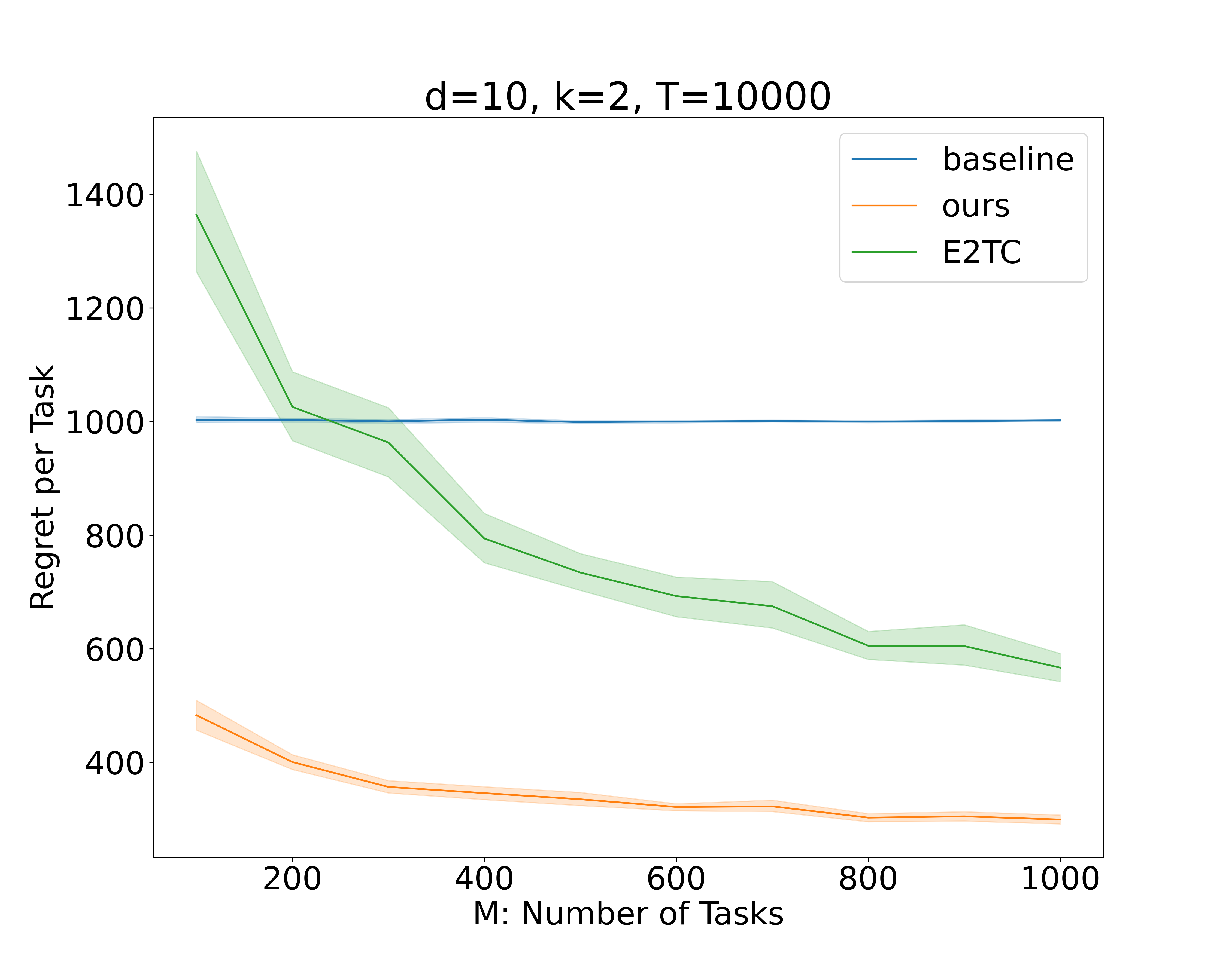
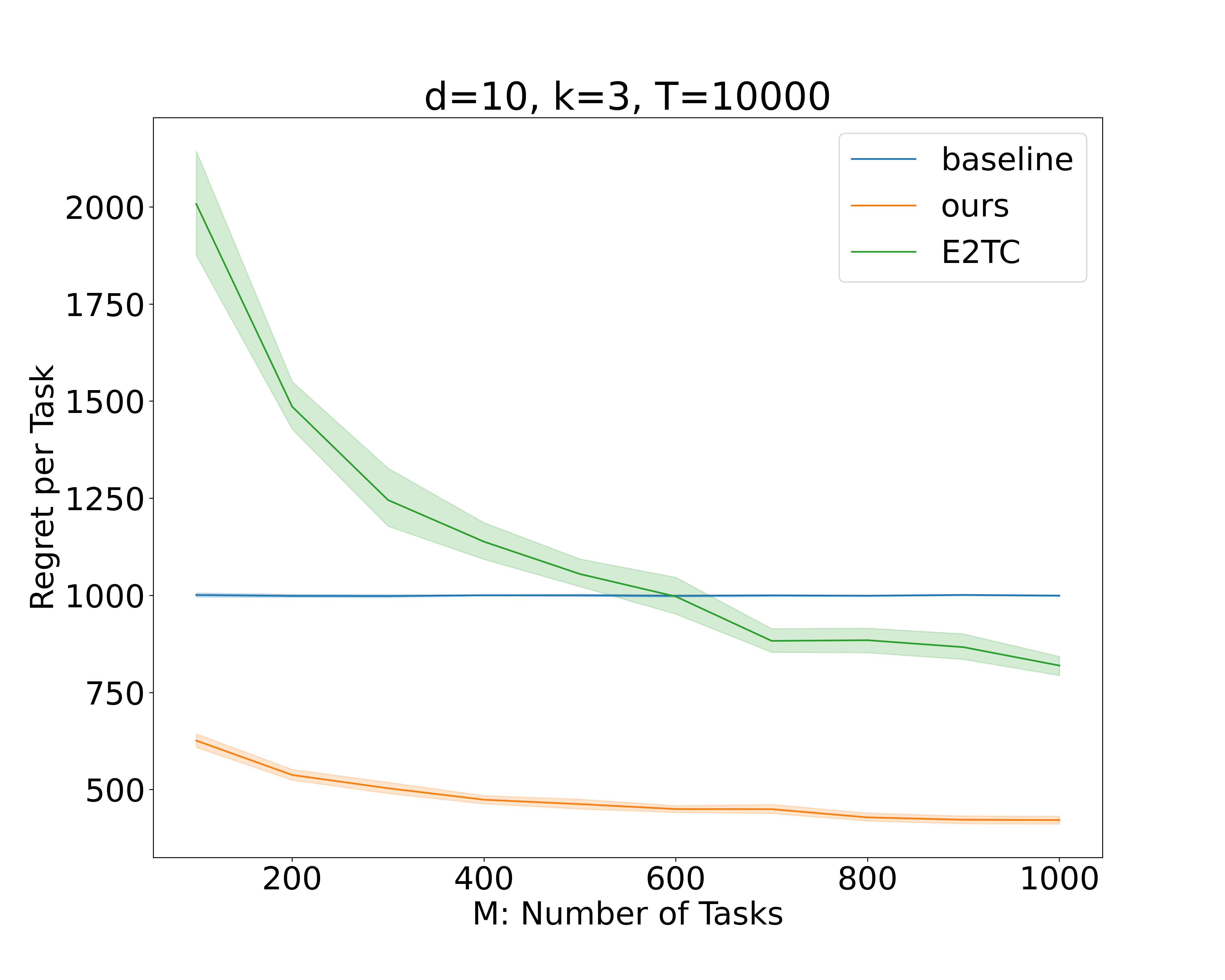
Figure 1: Comparisons of the E2TC algorithm in [Yang et al., 2021] and our Algorithm 1 for $k\in\{2,3,4\}$.

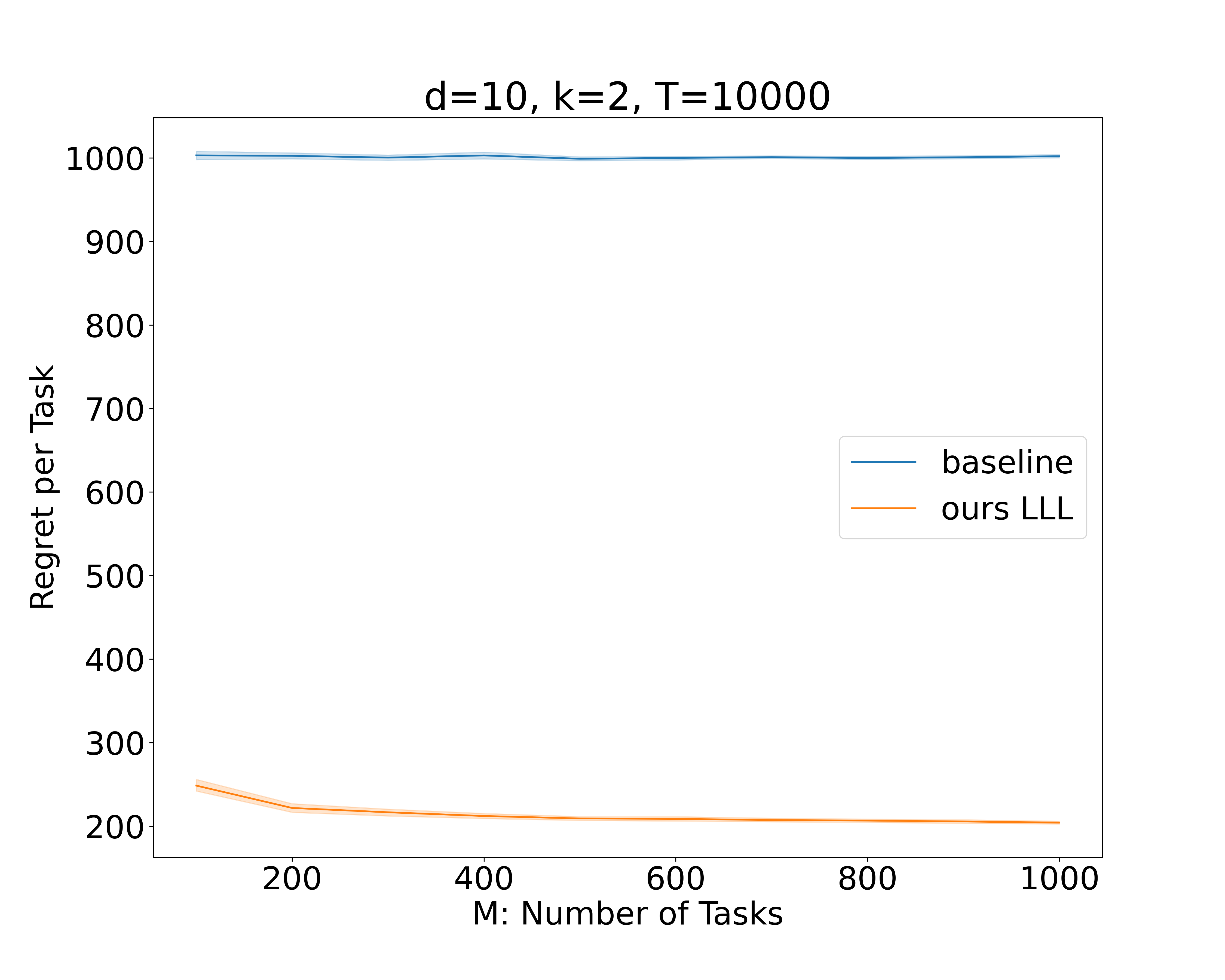
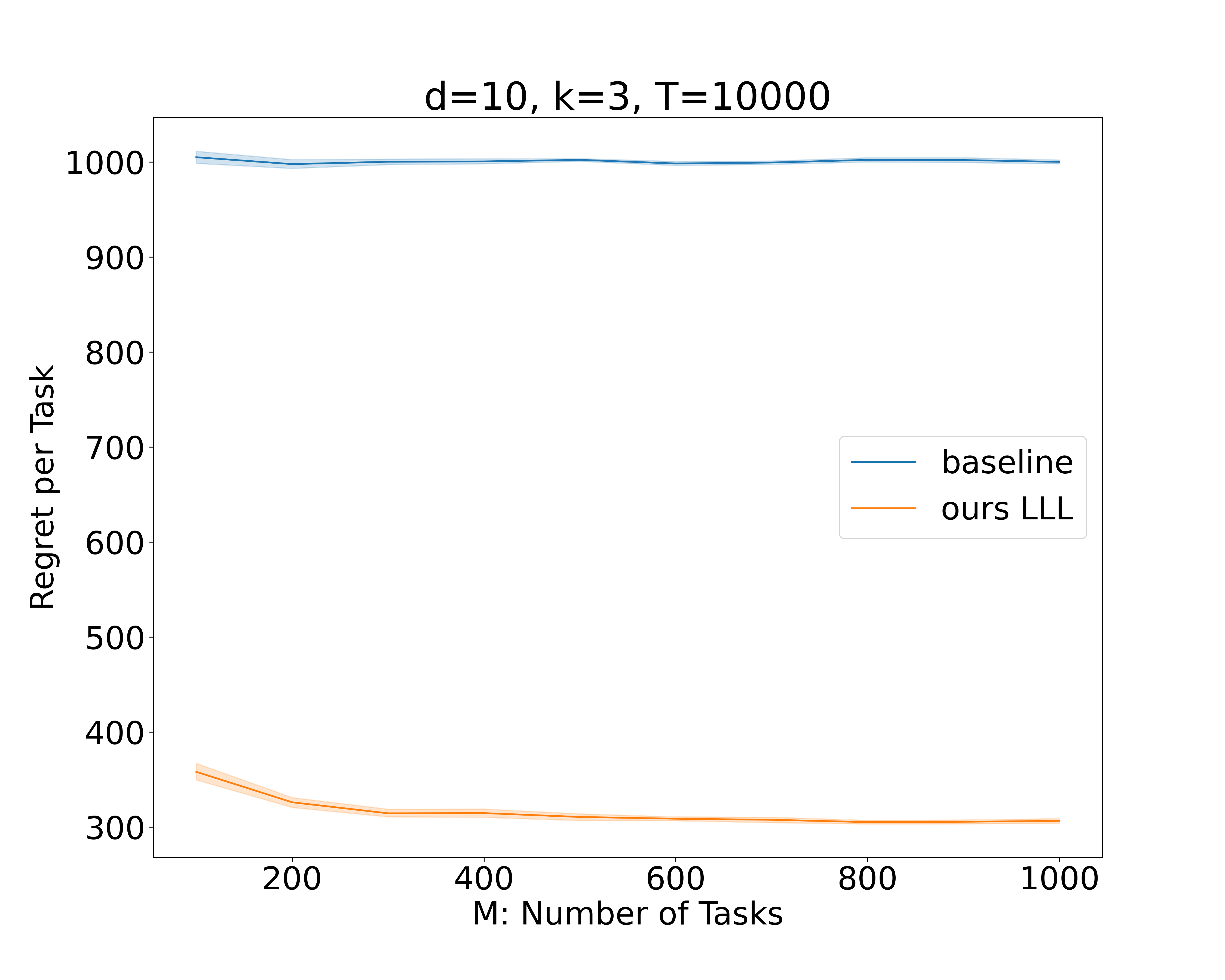
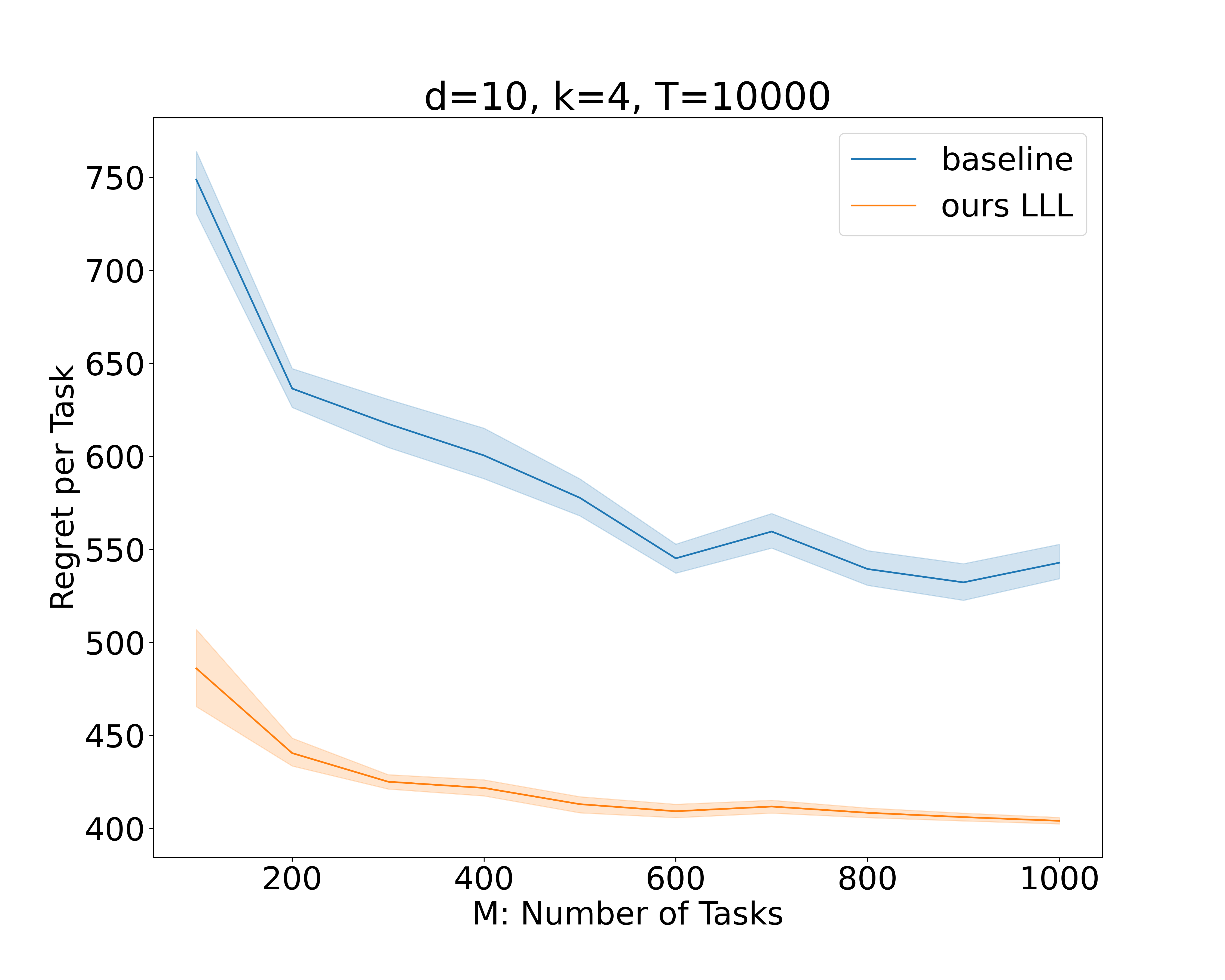
Figure 2: Comparisons of the naive baseline algorithm and our Algorithm 2 for $k\in\{2,3,4\}$.

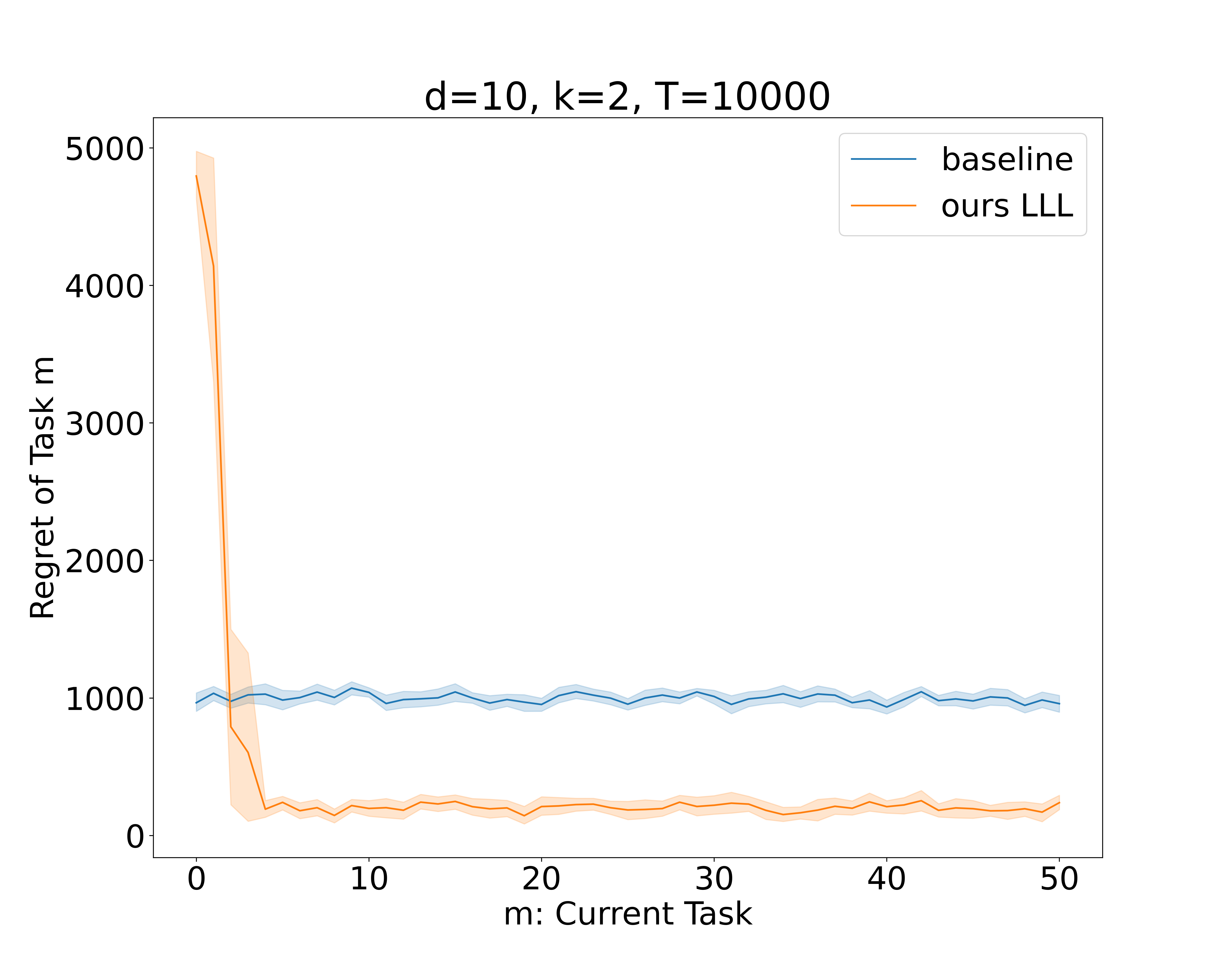
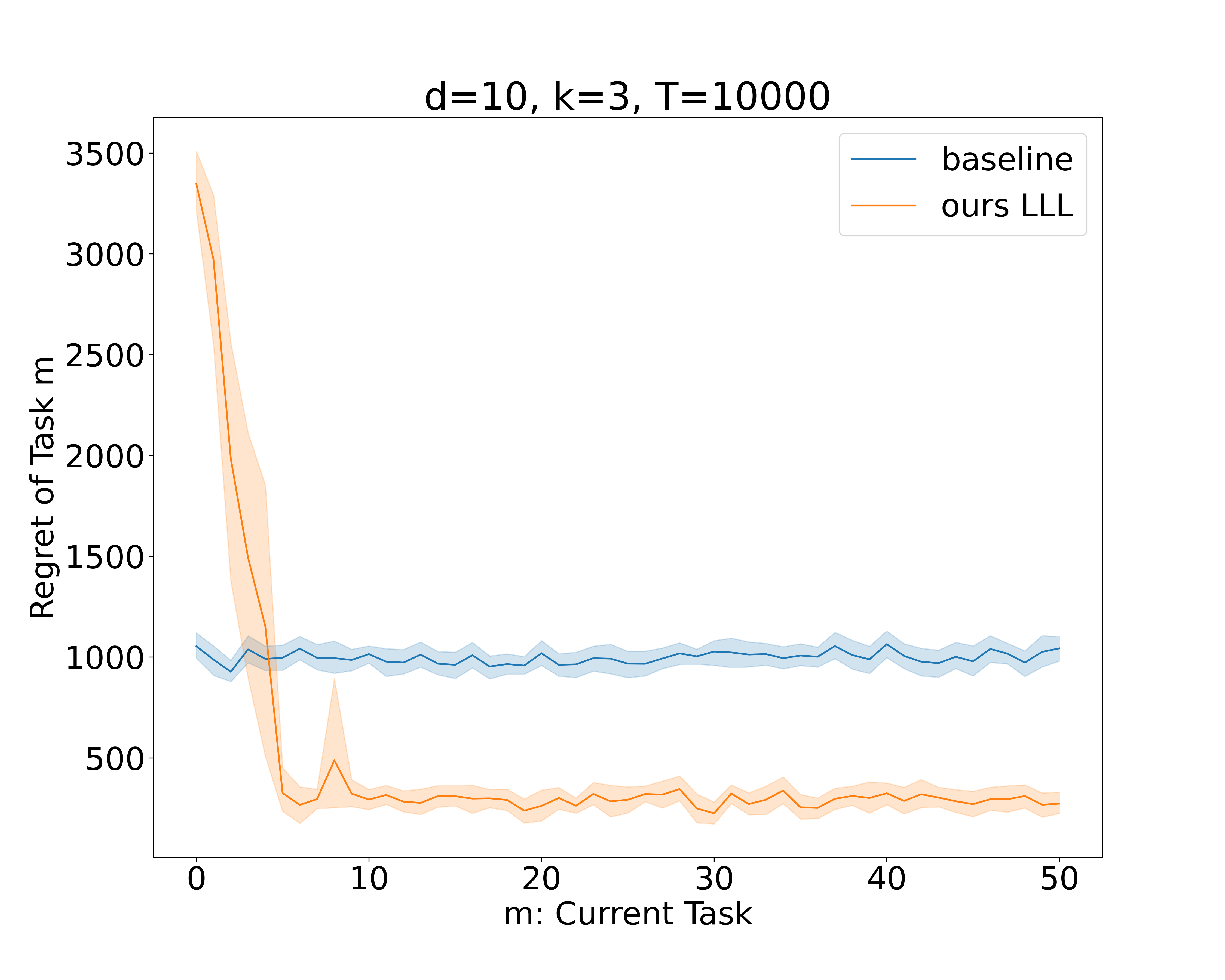
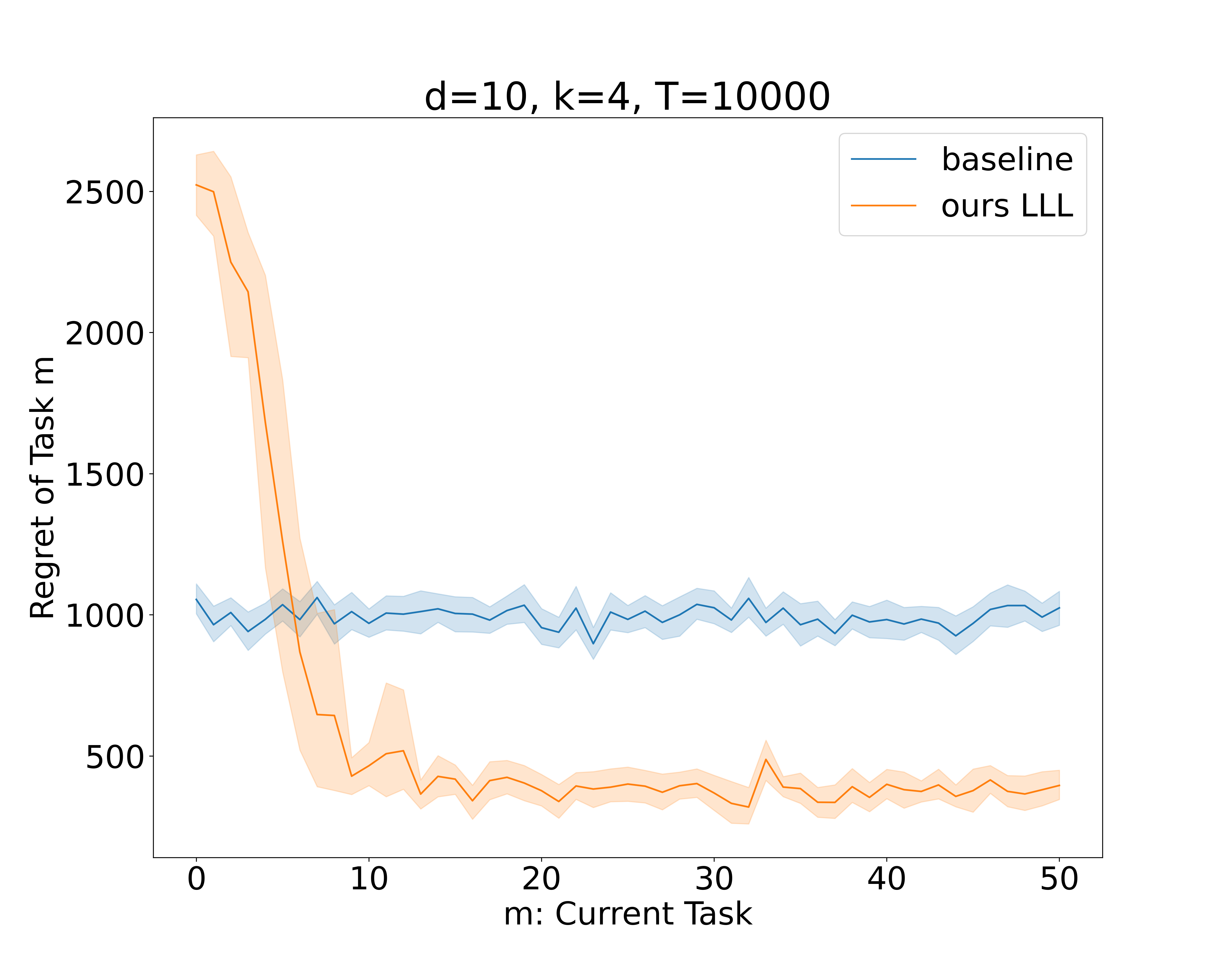
Figure 3: Comparisons of the naive baseline algorithm and our Algorithm 2 for $k\in\{2,3,4\}$.

Setup.

We run experiments on synthetic data. Following [Yang et al., 2021], we set $d=10,T=10^{4}$ and we consider $k=2,3,4$ in our experiments. ${\bm{B}}$ is generated by taking the first $k$ columns of a uniformly random orthonormal matrix, and each ${\bm{w}}_{m}$ is generated uniformly from sphere.

Results for the Multi-Task Setting.

We compare our algorithm with the baseline algorithm which treats each task independently, and the E2TC algorithm in [Yang et al., 2021]. The results are shown in Figure 1. For all settings, our algorithm achieves smaller regret, demonstrating the effectiveness of our new estimator.

Results for the Lifelong Setting.

Since lifelong linear bandits is a new setting, we only compare our algorithm, LLL, with the naive baseline algorithm which treats each task independently. In Figure 2, we vary the number of total tasks and report the per task regret. We observe that our algorithm significantly outperforms the base and its per task regret decreases as we increase the number of tasks, which matches our theory. In Figure 3, we report the regret on every task $m$ for in total $50$ tasks. We observe that for the initial tasks, we incur a higher regret than the baseline. However, the regret for later tasks is significantly smaller than the baseline. This matches our theory which indicates that after learning a good low-dimensional representation in the beginning, it benefits the efficiency in later tasks and reduces the regret.

7 Conclusion

In this paper, we gave near-optimal algorithms for multi-task and lifelong linear bandits with shared representation. A natural future direction is extend our algorithm to general representations, such as deep neural networks. Another interesting direction is to design optimal algorithms for multi-task reinforcement learning with shared representation.

Appendix A Technical Lemmas and Omitted Proofs

The following matrix Bernstein inequality is a straightforward corollary of Theorem 6.1.1 in [Tropp et al., 2015].

Lemma A.1.

Let ${\bm{A}}_{1},\cdots,{\bm{A}}_{n}\in{\mathbb{R}}^{d\times k}$ be a sequence of i.i.d. random matrices, such that $\mathbb{E}{\bm{A}}_{i}=0$ and $\norm{{\bm{A}}_{i}}\leq b$ for every $i\in[n]$. Let $\norm{\cdot}$ be the spectral norm of matrices. Let

$$v=\max_{i}\{\norm{\mathbb{E}[{\bm{A}}_{i}{\bm{A}}_{i}^{\top}]},\norm{\mathbb{E}[{\bm{A}}_{i}^{\top}{\bm{A}}_{i}]}\},$$ (36)

then with probability $1-O(\delta)$,

$$\norm{\frac{1}{n}\sum_{i=1}^{n}{\bm{A}}_{i}}\leq O(\sqrt{\frac{v\log\frac{d+k}{\delta}}{n}}+\frac{b\log\frac{d+k}{\delta}}{n}).$$ (37)

Lemma A.2 (Hoeffding [1963]).

Let $X_{1},\cdots,X_{n}$ be a sequence of i.i.d. random variables, such that $\mathbb{E}X_{i}=0$ and $\absolutevalue{X_{i}}\leq b$ for every $i\in[n]$. Then with probability $1-\delta$,

$$\absolutevalue{\frac{1}{n}\sum_{i=1}^{n}X_{i}}\leq b\sqrt{\frac{\log\frac{2}{\delta}}{n}}.$$ (38)

Lemma A.3 (Yang et al. [2021], Lemma 17).

Under Assumption ?, we have

$$1-\langle{\bm{a}}_{m},{\bm{\theta}}_{m}\rangle\leq\frac{\norm{{\bm{a}}_{m}-{\bm{\theta}}_{m}}_{2}^{2}}{\norm{{\bm{\theta}}_{m}}}.$$ (39)

Lemma A.4 (Yang et al. [2021], Lemma 18 applied to our setting).

$\mathbb{E}\norm{{\widehat{{\bm{\theta}}}}_{m}-{\bm{\theta}}_{m}}^{2}\leq O\left(\frac{k^{2}}{T_{2}}\right)+\norm{{\widehat{{\bm{B}}}}^{\top}_{\perp}{\bm{B}}}^{2}$.

Lemma A.5 (Elliptical potential lemma, Abbasi-Yadkori et al. [2011], Lemma 11).

Let ${\bm{x}}_{1},\cdots,{\bm{x}}_{n}\in{\mathbb{R}}^{d}$ be a sequence of vectors and let ${\bm{\Lambda}}_{i}=\lambda{\bm{I}}+\sum_{j=1}^{i}{\bm{x}}_{j}{\bm{x}}_{j}^{\top}$. Assume $\norm{{\bm{x}}_{i}}\leq\lambda$. Then

$$\sum_{i=1}^{n}\min\{1,\norm{{\bm{x}}_{i}}_{{\bm{\Lambda}}_{i-1}^{-1}}^{2}\}\leq 2\ln\frac{\det{\bm{\Lambda}}_{n}}{\det{\bm{\Lambda}}_{0}}\leq 2d\ln\frac{\tr{\bm{\Lambda}}_{n}+n}{\lambda}.$$ (40)

Proof of Theorem 5.2.

By 5.1, the regret can be bounded by

$$\quad{\widetilde{O}}(\frac{d^{2}k+k^{2}M}{\epsilon^{2}})+\sum_{m=1}^{M}\sum_{t=1}^{T}\max_{{\bm{a}}\in{\mathcal{A}}}\langle{\bm{a}}-{\bm{a}}_{t,m},{\bm{\theta}}_{m}\rangle$$

$$\leq{\widetilde{O}}(\frac{d^{2}k+k^{2}M}{\epsilon^{2}})+\sum_{m=1}^{M}T\cdot O(\norm{{\widehat{{\bm{\theta}}}}_{m}-{\bm{\theta}}_{m}}^{2})$$ (41)

$$\leq{\widetilde{O}}(\frac{d^{2}k+k^{2}M}{\epsilon^{2}})+O(MT\epsilon^{2})$$ (42)

$$\leq{\widetilde{O}}(d\sqrt{kMT}+kM\sqrt{T}),$$ (43)

where (43) is by choosing the optimal $\epsilon^{2}={\widetilde{O}}(\sqrt{(d^{2}k+k^{2}M)/MT})$. ∎

Proof of Lemma 5.3.

First, we note that ${\widehat{{\bm{B}}}}_{m}$ always have orthogonal columns by induction, because by equation 20, the last column ${\widehat{{\bm{b}}}}_{\tau_{m}}\propto{\bm{P}}^{\perp}_{{\widehat{{\bm{B}}}}_{m-1}}{\widehat{{\bm{\theta}}}}_{m}$ is always orthogonal to the first $\tau_{m}-1$ columns, which is ${\widehat{{\bm{B}}}}_{m-1}$.

Next, note that for $t\in[(j-1)n_{m,1}+1,jn_{m,1}]$, we have $\mathbb{E}[r_{t,m}]=\langle{\widehat{{\bm{B}}}}_{m-1}(j),{\bm{\theta}}_{m}\rangle$. Therefore, conditioned on $\tau_{m-1}$, by A.2, for each $j\in[\tau_{m-1}]$, with probability $1-\frac{\delta}{dM}$,

$$\absolutevalue{{\widetilde{\bm{w}}}_{m}(j)-\langle{\widehat{{\bm{B}}}}_{m-1}(j),{\bm{\theta}}_{m}\rangle}\leq\sqrt{\frac{\log\frac{2dM}{\delta}}{n_{m,1}}}.$$ (44)

By a union bound over $j\in[\tau_{m-1}]$, with probability $1-\frac{\delta}{M}$, (44) holds for every $j\in[\tau_{m-1}]$. Note that $\langle{\widetilde{\bm{\theta}}}_{m},{\widehat{{\bm{B}}}}_{m-1}(j)\rangle={\widetilde{\bm{w}}}_{m}(j)$, so with probability $1-\frac{\delta}{M}$,

$$\quad\norm{{\widetilde{\bm{\theta}}}_{m}-{\bm{P}}_{{\widehat{{\bm{B}}}}_{m-1}}{\bm{\theta}}_{m}}$$

$$=\sqrt{\sum_{j=1}^{\tau_{m-1}}\langle{\widehat{{\bm{B}}}}_{m-1}(j),{\widetilde{\bm{\theta}}}_{m}-{\bm{\theta}}_{m}\rangle^{2}}$$ (45)

$$\leq\sqrt{\sum_{j=1}^{\tau_{m-1}}\frac{\log\frac{2dM}{\delta}}{n_{m,1}}}$$ (46)

$$\leq\sqrt{\frac{\tau_{m-1}\log\frac{2dM}{\delta}}{n_{m,1}}},$$ (47)

where (45) uses that ${\widehat{{\bm{B}}}}_{m-1}$ has orthogonal columns. Finally, we conclude by a union bound over $m\in[M]$. ∎

Proof of Lemma 5.4.

We have

$$\quad\norm{{\bm{P}}_{{\widehat{{\bm{B}}}}_{m-1}}^{\perp}{\bm{\theta}}_{m}}$$

$$=\norm{{\bm{\theta}}_{m}-{\bm{P}}_{{\widehat{{\bm{B}}}}_{m-1}}{\bm{\theta}}_{m}}$$ (48)

$$\geq\norm{{\bm{\theta}}_{m}}-\norm{{\bm{P}}_{{\widehat{{\bm{B}}}}_{m-1}}{\bm{\theta}}_{m}}$$ (49)

$$\geq 1-(\norm{{\widetilde{\bm{\theta}}}_{m}}+\norm{{\widetilde{\bm{\theta}}}_{m}-{\bm{P}}_{{\widehat{{\bm{B}}}}_{m-1}}{\bm{\theta}}_{m}})$$ (50)

$$\geq\frac{\epsilon}{2},$$ (51)

where equation 51 is by 5.3 and by plugging in $n_{m,1}$. ∎

Proof of Lemma 5.5.

Note that $\nu_{\ell}=m$ and $\tau_{m}=\ell$. By A.2, for each $j\in[d]$, condition on $\nu_{\ell}=m$, with probability $1-\frac{\delta}{dM}$,

$$\absolutevalue{{\widehat{{\bm{\theta}}}}_{m}(j)-{\bm{\theta}}_{m}(j)}\leq\sqrt{\frac{\log\frac{2dM}{\delta}}{n_{m,2}}}.$$ (52)

By a union bound over $j\in[d]$, with probability $1-\frac{\delta}{M}$, (52) holds for every $j\in[d]$. Then

$$\norm{{\bm{\theta}}_{m}-{\widehat{{\bm{\theta}}}}_{m}} =\sqrt{\sum_{j=1}^{d}({\widehat{{\bm{\theta}}}}_{m}(j)-{\bm{\theta}}_{m}(j))^{2}}$$ (53)

$$\leq\sqrt{\sum_{j=1}^{d}\frac{\log\frac{2dM}{\delta}}{n_{m,2}}}$$ (54)

$$=\sqrt{\frac{d\log\frac{2dM}{\delta}}{n_{m,2}}},$$ (55)

Furthermore, because ${\bm{P}}_{{\bm{B}}}{\bm{\theta}}_{m}={\bm{\theta}}_{m}$, we have $\norm{{\bm{\theta}}_{m}-{\widehat{{\bm{b}}}}_{\tau_{m}}}=\norm{{\bm{P}}_{{\bm{B}}}({\bm{\theta}}_{m}-{\widehat{{\bm{\theta}}}}_{m})}\leq\norm{{\bm{\theta}}_{m}-{\widehat{{\bm{\theta}}}}_{m}}$. Finally, we note that

$$\norm{{\bm{d}}_{\tau_{m}}} =\norm{{\bm{P}}^{\perp}_{{\bm{B}}}{\widehat{{\bm{\theta}}}}_{m}}$$

$$=\norm{{\bm{P}}^{\perp}_{{\bm{B}}}({\widehat{{\bm{\theta}}}}_{m}-{\bm{\theta}}_{m})}\leq\norm{{\widehat{{\bm{\theta}}}}_{m}-{\bm{\theta}}_{m}},$$ (56)

and we conclude by a union bound over $\ell\leq M$. ∎

Lemma A.6.

Let $\kappa=d\log\frac{d}{\delta}$. Define the event ${\mathcal{E}}_{3}=\{{\bm{D}}_{\kappa}^{\top}{\bm{D}}_{\kappa}\preccurlyeq\epsilon^{2}{\bm{I}}\}$. Then $\Pr[{\mathcal{E}}_{3}]\geq 1-\delta$.

Proof.

Define the $\sigma$-field ${\mathcal{F}}_{\ell}=\sigma(\tau_{1},\cdots,\tau_{\ell})$. Then ${\mathcal{F}}=\{{\mathcal{F}}_{1}\subseteq{\mathcal{F}}_{2}\subseteq\cdots\}$ is a filtration. Note that ${\bm{d}}_{1},{\bm{d}}_{2},\cdots,{\bm{d}}_{\kappa}$ is a stochastic process adapted to the filtration ${\mathcal{F}}$, and that ${\bm{D}}_{\kappa}^{\top}{\bm{D}}_{\kappa}=\sum_{\ell=1}^{\kappa}{\bm{d}}_{\ell}{\bm{d}}_{\ell}^{\top}$. Furthermore, we note that ${\bm{d}}_{\ell}\mid{\mathcal{F}}_{\ell}\sim{\mathcal{N}}(0,\frac{1}{n_{m,2}}{\bm{I}})$, so by Lemma A.1, with probability $1-\delta$,

$$\norm{\sum_{\ell=1}^{\kappa}{\bm{d}}_{\ell}{\bm{d}}_{\ell}^{\top}-\frac{1}{n_{m,2}}{\bm{I}}}\leq O(\sqrt{\frac{\kappa}{n_{m,2}}\log\frac{d}{\delta}}).$$ (57)

∎

References

• Abbasi-Yadkori et al. [2011] Yasin Abbasi-Yadkori, Dávid Pál, and Csaba Szepesvári. Improved algorithms for linear stochastic bandits. In Advances in Neural Information Processing Systems, pages 2312–2320, 2011.
• Alquier et al. [2016] Pierre Alquier, The Tien Mai, and Massimiliano Pontil. Regret bounds for lifelong learning. arXiv preprint arXiv:1610.08628, 2016.
• Ando and Zhang [2005] Rie Kubota Ando and Tong Zhang. A framework for learning predictive structures from multiple tasks and unlabeled data. Journal of Machine Learning Research, 6(Nov):1817–1853, 2005.
• Arora et al. [2019] Sanjeev Arora, Hrishikesh Khandeparkar, Mikhail Khodak, Orestis Plevrakis, and Nikunj Saunshi. A theoretical analysis of contrastive unsupervised representation learning. In Proceedings of the 36th International Conference on Machine Learning, 2019.
• Arora et al. [2020] Sanjeev Arora, Simon S Du, Sham Kakade, Yuping Luo, and Nikunj Saunshi. Provable representation learning for imitation learning via bi-level optimization. arXiv preprint arXiv:2002.10544, 2020.
• Auer [2002] Peter Auer. Using confidence bounds for exploitation-exploration trade-offs. Journal of Machine Learning Research, 3(Nov):397–422, 2002.
• Bastani et al. [2019] Hamsa Bastani, David Simchi-Levi, and Ruihao Zhu. Meta dynamic pricing: Learning across experiments. arXiv preprint arXiv:1902.10918, 2019.
• Baxter [2000] Jonathan Baxter. A model of inductive bias learning. Journal of artificial intelligence research, 12:149–198, 2000.
• Ben-David and Schuller [2003] Shai Ben-David and Reba Schuller. Exploiting task relatedness for multiple task learning. In Learning Theory and Kernel Machines, pages 567–580. Springer, 2003.
• Bengio et al. [2013] Yoshua Bengio, Aaron Courville, and Pascal Vincent. Representation learning: A review and new perspectives. IEEE transactions on pattern analysis and machine intelligence, 35(8):1798–1828, 2013.
• Bertinetto et al. [2018] Luca Bertinetto, Joao F Henriques, Philip HS Torr, and Andrea Vedaldi. Meta-learning with differentiable closed-form solvers. arXiv preprint arXiv:1805.08136, 2018.
• Cai and Zhang [2018] T Tony Cai and Anru Zhang. Rate-optimal perturbation bounds for singular subspaces with applications to high-dimensional statistics. The Annals of Statistics, 46(1):60–89, 2018.
• Cao et al. [2021] Xinyuan Cao, Weiyang Liu, and Santosh S Vempala. Provable lifelong learning of representations. arXiv preprint arXiv:2110.14098, 2021.
• Caruana [1997] Rich Caruana. Multitask learning. Machine learning, 28(1):41–75, 1997.
• Cavallanti et al. [2010] Giovanni Cavallanti, Nicolo Cesa-Bianchi, and Claudio Gentile. Linear algorithms for online multitask classification. Journal of Machine Learning Research, 11(Oct):2901–2934, 2010.
• Chu et al. [2011] Wei Chu, Lihong Li, Lev Reyzin, and Robert Schapire. Contextual bandits with linear payoff functions. In Proceedings of the Fourteenth International Conference on Artificial Intelligence and Statistics, pages 208–214, 2011.
• Dani et al. [2008] Varsha Dani, Thomas P. Hayes, and Sham M. Kakade. Stochastic linear optimization under bandit feedback. In COLT, 2008.
• Denevi et al. [2018] Giulia Denevi, Carlo Ciliberto, Dimitris Stamos, and Massimiliano Pontil. Incremental learning-to-learn with statistical guarantees. arXiv preprint arXiv:1803.08089, 2018.
• Denevi et al. [2019] Giulia Denevi, Carlo Ciliberto, Riccardo Grazzi, and Massimiliano Pontil. Learning-to-learn stochastic gradient descent with biased regularization. In Proceedings of the 36th International Conference on Machine Learning, 2019.
• D’Eramo et al. [2020] Carlo D’Eramo, Davide Tateo, Andrea Bonarini, Marcello Restelli, and Jan Peters. Sharing knowledge in multi-task deep reinforcement learning. In International Conference on Learning Representations, 2020. URL https://openreview.net/forum?id=rkgpv2VFvr.
• Deshmukh et al. [2017] Aniket Anand Deshmukh, Urun Dogan, and Clay Scott. Multi-task learning for contextual bandits. In Advances in neural information processing systems, pages 4848–4856, 2017.
• Du et al. [2020] Simon S Du, Wei Hu, Sham M Kakade, Jason D Lee, and Qi Lei. Few-shot learning via learning the representation, provably. arXiv preprint arXiv:2002.09434, 2020.
• Finn et al. [2019] Chelsea Finn, Aravind Rajeswaran, Sham Kakade, and Sergey Levine. Online meta-learning. In Proceedings of the 36th International Conference on Machine Learning, 2019.
• Galanti et al. [2016] Tomer Galanti, Lior Wolf, and Tamir Hazan. A theoretical framework for deep transfer learning. Information and Inference: A Journal of the IMA, 5(2):159–209, 2016.
• Hessel et al. [2019] Matteo Hessel, Hubert Soyer, Lasse Espeholt, Wojciech Czarnecki, Simon Schmitt, and Hado van Hasselt. Multi-task deep reinforcement learning with popart. In Proceedings of the AAAI Conference on Artificial Intelligence, volume 33, pages 3796–3803, 2019.
• Higgins et al. [2017] Irina Higgins, Arka Pal, Andrei Rusu, Loic Matthey, Christopher Burgess, Alexander Pritzel, Matthew Botvinick, Charles Blundell, and Alexander Lerchner. Darla: Improving zero-shot transfer in reinforcement learning. In Proceedings of the 34th International Conference on Machine Learning-Volume 70, pages 1480–1490. JMLR. org, 2017.
• Hoeffding [1963] Wassily Hoeffding. Probability inequalities for sums of bounded random variables. Journal of the American Statistical Association, 58(301):13–30, 1963.
• Hu et al. [2021] Jiachen Hu, Xiaoyu Chen, Chi Jin, Lihong Li, and Liwei Wang. Near-optimal representation learning for linear bandits and linear rl. In International Conference on Machine Learning, pages 4349–4358. PMLR, 2021.
• Huang et al. [2021] Baihe Huang, Kaixuan Huang, Sham M Kakade, Jason D Lee, Qi Lei, Runzhe Wang, and Jiaqi Yang. Optimal gradient-based algorithms for non-concave bandit optimization. arXiv preprint arXiv:2107.04518, 2021.
• Jun et al. [2019] Kwang-Sung Jun, Rebecca Willett, Stephen Wright, and Robert Nowak. Bilinear bandits with low-rank structure. In International Conference on Machine Learning, pages 3163–3172, 2019.
• Khodak et al. [2019] Mikhail Khodak, Maria-Florina Balcan, and Ameet Talwalkar. Adaptive gradient-based meta-learning methods. arXiv preprint arXiv:1906.02717, 2019.
• Lale et al. [2019] Sahin Lale, Kamyar Azizzadenesheli, Anima Anandkumar, and Babak Hassibi. Stochastic linear bandits with hidden low rank structure. arXiv preprint arXiv:1901.09490, 2019.
• Lattimore and Hao [2021] Tor Lattimore and Botao Hao. Bandit phase retrieval. arXiv preprint arXiv:2106.01660, 2021.
• Lazaric and Restelli [2011] Alessandro Lazaric and Marcello Restelli. Transfer from multiple mdps. In Advances in Neural Information Processing Systems, pages 1746–1754, 2011.
• Lee et al. [2019] Kwonjoon Lee, Subhransu Maji, Avinash Ravichandran, and Stefano Soatto. Meta-learning with differentiable convex optimization. In Proceedings of the IEEE Conference on Computer Vision and Pattern Recognition, pages 10657–10665, 2019.
• Li et al. [2014] Jiayi Li, Hongyan Zhang, Liangpei Zhang, Xin Huang, and Lefei Zhang. Joint collaborative representation with multitask learning for hyperspectral image classification. IEEE Transactions on Geoscience and Remote Sensing, 52(9):5923–5936, 2014.
• Li et al. [2019a] Yingkai Li, Yining Wang, and Yuan Zhou. Nearly minimax-optimal regret for linearly parameterized bandits. In Conference on Learning Theory, pages 2173–2174, 2019a.
• Li et al. [2019b] Yingkai Li, Yining Wang, and Yuan Zhou. Tight regret bounds for infinite-armed linear contextual bandits. arXiv preprint arXiv:1905.01435, 2019b.
• Liu et al. [2016] Lydia T Liu, Urun Dogan, and Katja Hofmann. Decoding multitask dqn in the world of minecraft. In The 13th European Workshop on Reinforcement Learning (EWRL) 2016, 2016.
• Liu et al. [2019] Tianyi Liu, Minshuo Chen, Mo Zhou, Simon S Du, Enlu Zhou, and Tuo Zhao. Towards understanding the importance of shortcut connections in residual networks. In H. Wallach, H. Larochelle, A. Beygelzimer, F. d'Alché-Buc, E. Fox, and R. Garnett, editors, Advances in Neural Information Processing Systems, volume 32. Curran Associates, Inc., 2019. URL https://proceedings.neurips.cc/paper/2019/file/7716d0fc31636914783865d34f6cdfd5-Paper.pdf.
• Lu et al. [2021] Rui Lu, Gao Huang, and Simon S Du. On the power of multitask representation learning in linear mdp. arXiv preprint arXiv:2106.08053, 2021.
• Lu et al. [2020] Yangyi Lu, Amirhossein Meisami, and Ambuj Tewari. Low-rank generalized linear bandit problems. arXiv preprint arXiv:2006.02948, 2020.
• Maurer [2006] Andreas Maurer. Bounds for linear multi-task learning. Journal of Machine Learning Research, 7(Jan):117–139, 2006.
• Maurer et al. [2016] Andreas Maurer, Massimiliano Pontil, and Bernardino Romera-Paredes. The benefit of multitask representation learning. The Journal of Machine Learning Research, 17(1):2853–2884, 2016.
• McNamara and Balcan [2017] Daniel McNamara and Maria-Florina Balcan. Risk bounds for transferring representations with and without fine-tuning. In Proceedings of the 34th International Conference on Machine Learning-Volume 70, pages 2373–2381. JMLR. org, 2017.
• Modi et al. [2021] Aditya Modi, Mohamad Kazem Shirani Faradonbeh, Ambuj Tewari, and George Michailidis. Joint learning of linear time-invariant dynamical systems. arXiv preprint arXiv:2112.10955, 2021.
• Parisotto et al. [2015] Emilio Parisotto, Jimmy Lei Ba, and Ruslan Salakhutdinov. Actor-mimic: Deep multitask and transfer reinforcement learning. arXiv preprint arXiv:1511.06342, 2015.
• Qin et al. [2022] Yuzhen Qin, Tommaso Menara, Samet Oymak, ShiNung Ching, and Fabio Pasqualetti. Non-stationary representation learning in sequential linear bandits. arXiv preprint arXiv:2201.04805, 2022.
• Ramsundar et al. [2015] Bharath Ramsundar, Steven Kearnes, Patrick Riley, Dale Webster, David Konerding, and Vijay Pande. Massively multitask networks for drug discovery. arXiv preprint arXiv:1502.02072, 2015.
• Rusmevichientong and Tsitsiklis [2010] Paat Rusmevichientong and John N Tsitsiklis. Linearly parameterized bandits. Mathematics of Operations Research, 35(2):395–411, 2010.
• Rusu et al. [2015] Andrei A Rusu, Sergio Gomez Colmenarejo, Caglar Gulcehre, Guillaume Desjardins, James Kirkpatrick, Razvan Pascanu, Volodymyr Mnih, Koray Kavukcuoglu, and Raia Hadsell. Policy distillation. arXiv preprint arXiv:1511.06295, 2015.
• Soare et al. [2018] Marta Soare, Ouais Alsharif, Alessandro Lazaric, and Joelle Pineau. Multi-task linear bandits. 2018.
• Taylor and Stone [2009] Matthew E Taylor and Peter Stone. Transfer learning for reinforcement learning domains: A survey. Journal of Machine Learning Research, 10(Jul):1633–1685, 2009.
• Teh et al. [2017] Yee Teh, Victor Bapst, Wojciech M Czarnecki, John Quan, James Kirkpatrick, Raia Hadsell, Nicolas Heess, and Razvan Pascanu. Distral: Robust multitask reinforcement learning. In Advances in Neural Information Processing Systems, pages 4496–4506, 2017.
• Thekumparampil et al. [2021] Kiran Koshy Thekumparampil, Prateek Jain, Praneeth Netrapalli, and Sewoong Oh. Sample efficient linear meta-learning by alternating minimization. arXiv preprint arXiv:2105.08306, 2021.
• Tripuraneni et al. [2020a] Nilesh Tripuraneni, Chi Jin, and Michael I Jordan. Provable meta-learning of linear representations. arXiv preprint arXiv:2002.11684, 2020a.
• Tripuraneni et al. [2020b] Nilesh Tripuraneni, Michael I Jordan, and Chi Jin. On the theory of transfer learning: The importance of task diversity. arXiv preprint arXiv:2006.11650, 2020b.
• Tropp et al. [2015] Joel A Tropp et al. An introduction to matrix concentration inequalities. Foundations and Trends® in Machine Learning, 8(1-2):1–230, 2015.
• Yang et al. [2021] Jiaqi Yang, Wei Hu, Jason D Lee, and Simon S Du. Impact of representation learning in linear bandits. In International Conference on Learning Representations, 2021.