Temporal Robustness of Temporal Logic Specifications: Analysis and Control Design

Abstract.

We study the temporal robustness of temporal logic specifications and show how to design temporally robust control laws for time-critical control systems. This topic is of particular interest in connected systems and interleaving processes such as multi-robot and human-robot systems where uncertainty in the behavior of individual agents and humans can induce timing uncertainty. Despite the importance of time-critical systems, temporal robustness of temporal logic specifications has not been studied, especially from a control design point of view. We define synchronous and asynchronous temporal robustness and show that these notions quantify the robustness with respect to synchronous and asynchronous time shifts in the predicates of the temporal logic specification. It is further shown that the synchronous temporal robustness upper bounds the asynchronous temporal robustness. We then study the control design problem in which we aim to design a control law that maximizes the temporal robustness of a dynamical system. Our solution consists of a Mixed-Integer Linear Programming (MILP) encoding that can be used to obtain a sequence of optimal control inputs. While asynchronous temporal robustness is arguably more nuanced than synchronous temporal robustness, we show that control design using synchronous temporal robustness is computationally more efficient. This trade-off can be exploited by the designer depending on the particular application at hand. We conclude the paper with a variety of case studies.

1. Introduction

Time-critical systems are systems that need to satisfy stringent real-time constraints. Examples of time-critical systems include, but are not limited to, medical devices, autonomous driving, automated warehouses, and air traffic control systems. The reliability and safety of such time-critical systems greatly depends on being robust with respect to timing uncertainty. For instance, Germany’s rail network has become prone to frequent train delays which makes scheduling and planning a difficult task (Connolly, 2018). It is hence natural to study temporal robustness of time-critical systems, i.e., to study a system’s ability to be robust with respect to timing uncertainty.

Temporal logics provide a principled mechanism to express a broad range of real-time constraints that can be imposed on time-critical systems (Kress-Gazit et al., 2009; Kloetzer and Belta, 2008; Guo and Dimarogonas, 2015; Kantaros and Zavlanos, 2018). In fact, there exists a variety of temporal logics, all with their own merits, that have been explored from an analysis and control design point of view. However, the temporal robustness of systems under temporal logic specifications has not yet been studied and used for control design. An initial attempt to define temporal robustness was made in (Donzé and Maler, 2010) without, however, further analyzing properties of temporal robustness and without using it for control design. In fact, a natural objective is to design a system to be robust to previously mentioned timing uncertainties. This refers to the control design problem in which we aim to design a control law that maximizes the temporal robustness of a system. The control design problem has not been addressed before and is subject to numerical challenges as the temporal robustness semantics are not differentiable, so that gradient-based optimization methods fail to be applicable. To address this challenge, we presented a Mixed-Integer Linear Programming (MILP) encoding in our previous work (Rodionova et al., 2021) where we describe how to control a dynamical system in order to maximize its temporal robustness.

In this paper, we introduce and analyze the notions of synchronous and asynchronous temporal robustness. While the temporal robustness as presented in (Donzé and Maler, 2010) is similar to what we define as asynchronous temporal robustness, we provide a slightly modified definition and a detailed analysis of the synchronous and asynchronous temporal robustness. In particular, we show that these notions are sound in the sense that a positive (negative) robustness implies satisfaction (violation) of the specification in hand. Furthermore, we analyze the meaning of temporal robustness in terms of permissible time shifts in the predicates of the specification and in the underlying signal. For both notions we present MILP encodings, following ideas of our initial work in (Rodionova et al., 2021), that solves the control design problem in which we aim to maximize the synchronous and asynchronous temporal robustness.

1.1. Related Work

Time-critical systems have been studied in the literature dealing with real-time systems (Laplante et al., 2004; Liu, 2000). The design of task scheduling algorithms for real-time systems has been extensively studied, see e.g., (Sha et al., 2004) for an overview. Scheduling algorithms aim at finding an execution order for a set of tasks with corresponding deadlines. Solutions consist, for instance, of periodic scheduling (Serafini and Ukovich, 1989) and of event triggered scheduling (Tabuada, 2007). While these scheduling algorithms are useful in control design, no consideration has been given to the temporal robustness of the system. Hence we view these works as complementary.

Another direction in the study of real-time systems are timed automata as a modeling formalism (Alur and Dill, 1994; Bengtsson and Yi, 2003). Timed automata allow automatic verification using model checking tools such as UPPAAL (Behrmann et al., 2004). Robustness of timed automata was investigated in (Gupta et al., 1997) and (Bendík et al., 2021), while control of timed automata was considered in (Maler et al., 1995) and (Asarin et al., 1998). A connection between the aforementioned scheduling and timed automata was made in (Fersman et al., 2006).

Interestingly, timed automata have been connected to temporal logics. Particularly, it has been shown that every Metric Interval Temporal Logic (MITL) formula can be translated into a language equivalent timed automaton (Alur and Henzinger, 1996). This means that the satisfiability of an MITL formula can be reduced to an emptiness checking problem of a timed automaton. Signal Temporal Logic (STL) (Maler and Nickovic, 2004a) is in spirit similar to MITL, but additionally allows to consider predicates instead of only propositions. It has been shown that STL formulas can be translated into a language equivalent timed signal transducer in (Lindemann and Dimarogonas, 2020).

Various notions of robustness have been presented for temporal logics. Spatial robustness of MITL specifications over deterministic signals was considered in (Donzé and Maler, 2010; Fainekos and Pappas, 2009b). Spatial robustness particularly allows to quantify permissible uncertainty of the signal for each point in time, e.g., caused by additive disturbances. Other notions of spatial robustness are the arithmetic-geometric integral mean robustness (Mehdipour et al., 2019) and the smooth cumulative robustness (Haghighi et al., 2019) as well as notions that are tailored for use in reinforcement learning applications (Varnai and Dimarogonas, 2020). Spatial robustness for stochastic systems was considered in (Bartocci et al., 2013, 2015) as well as in (Lindemann et al., 2021) when considering the risk of violating a specification. Control of dynamical systems under STL specifications has first been considered in (Raman et al., 2014) by means of an MILP encoding that allows to maximize spatial robustness. Other optimization-based methods that also follow the idea of maximizing spatial robustness have been proposed in (Mehdipour et al., 2019; Pant et al., 2018; Gilpin et al., 2020). Another direction has been to design transient feedback control laws that maximize the spatial robustness of fragments of STL specification (Lindemann and Dimarogonas, 2018) and (Charitidou and Dimarogonas, 2021).

Analysis and control design for STL specifications focuses mainly on spatial robustness, while less attention has been on temporal robustness of real-time systems. The authors in (Akazaki and Hasuo, 2015) proposed averaged STL that captures a form of temporal robustness by averaging over time intervals. Other forms of temporal robustness include the notion of system conformance to quantify closeness of systems in terms of spatial and temporal closeness of system trajectories (Abbas et al., 2014; Gazda and Mousavi, 2020; Deshmukh et al., 2015). Conformance, however, only allows to reason about temporal robustness with respect to synchronous time shifts of a signal and not with respect to synchronous and asynchronous time shifts as considered in this work. As remarked before, temporal robustness for STL specifications was initially presented without further analysis in (Donzé and Maler, 2010). Temporally-robust control has been considered in (Lin and Baras, 2020) for special fragments of STL, and in (Rodionova et al., 2021) for general fragments of STL using MILP encodings. In an orthogonal direction that is worth mentioning, the authors in (Penedo et al., 2020) and (Kamale et al., 2021) consider the problem of finding temporal relaxations for time window temporal logic specifications (Vasile et al., 2017).

1.2. Contributions and Paper Outline

When dealing with time-critical system, a natural objective is to analyze robustness to various forms of timing uncertainties and to design a control system to maximize this robustness. We consider the temporal robust interpretation of STL formulas over continuous and discrete-time signals. Our goal is to establish a comprehensive theoretical framework for temporal robustness of STL specifications which has not been studied before, especially from a control design point of view. We make the following contributions.

• We define synchronous and asynchronous temporal robustness to quantify the robustness with respect to synchronous and asynchronous time shifts in the predicates of the underlying signal temporal logic specification.

• We present various desirable properties of the presented robustness notions and show that the synchronous temporal robustness upper bounds the asynchronous temporal robustness in its absolute value. Moreover, we show under which conditions these two robustness notions are equivalent.

• We then study the control design problem in which we aim to design a control law that maximizes the temporal robustness of a dynamical system. To solve this problem, we present Mixed-Integer Linear Programming (MILP) encodings following ideas of our initial work in (Rodionova et al., 2021). We provide correctness guarantees and a complexity analysis of the encodings.

• All theoretical results are highlighted in three case studies. Particularly, we show how the proposed MILP encodings can be used to perform temporally-robust control of multi-agent systems.

The remainder of the paper is organized as follows. Section 2 provides background on STL. In Section 3, the synchronous and asynchronous temporal robustness is introduced. Soundness properties of temporal robustness are presented in Section 4 while the properties with respect to time shifts are presented in Section 5. In Section 6 we present MILP encodings to solve the temporally-robust control problem. Extensive simulations and case studies are presented in Section 7. Finally, we summarize with conclusions in Section 8.

2. Background on Signal Temporal Logic (STL)

Let $\mathbb{R}$ and $\mathbb{Z}$ be the set of real numbers and integers, respectively. Let $\mathbb{R}^{n}$ be the $n$-dimensional real vector space. The supremum operator is written as $\sqcup$ and the infimum operator is written as $\sqcap$. We define the set $\mathbb{B}:=\{\top,\bot\}$, where $\top$ and $\bot$ are the Boolean constants true and false, respectively. We also define the sign function as

$$\operatorname{sign}(x):=\begin{cases}1,&\text{if }x\geq 0\\ -1&\text{if }x<0.\end{cases}$$

In general, we say that a signal $\mathbf{x}$ is a map $\mathbf{x}:\mathbb{T}\to X$ where $\mathbb{T}$ is a time domain and where the state space $X$ is a metric space. In this work, we particularly consider the cases of real-valued continuous-time signals which naturally includes the case of discrete-time signals. In other words, the state space is $X\subseteq\mathbb{R}^{n}$ and the time domain is either $\mathbb{T}:=\mathbb{R}$ or $\mathbb{T}:=\mathbb{Z}$. For any set $\mathbb{T}$ we denote by $\overline{\mathbb{T}}=\mathbb{T}\cup\{\pm\infty\}$, for instance, $\overline{\mathbb{R}}:=\mathbb{R}\cup\{\pm\infty\}$ and $\overline{\mathbb{Z}}:=\mathbb{Z}\cup\{\pm\infty\}$ are the extended real numbers and integers, respectively. Finally, we denote the set of all signals $\mathbf{x}:\mathbb{T}\rightarrow X$ as the signal space $X^{\mathbb{T}}$.

2.1. Signal Temporal Logic

For a signal $\mathbf{x}:\mathbb{T}\to X$, let the signal state at time step $t$ be $x_{t}\in X$. Let $\mu:X\to\mathbb{R}$ be a real-valued function and let $p:X\to\mathbb{B}$ be a predicate defined via $\mu$ as $p(x):=\mu(x)\geq 0$. Thus, a predicate $\mu$ defines a set in which $p$ holds true, namely $p$ defines the set $\{x\in X\;|\;\mu(x)\geq 0\}$ in which $p$ is true. Let $AP:=\{p_{1},\ldots,p_{L}\}$ be a set of $L$ predicates defined via the set of predicate functions $M:=\{\mu_{1},\ldots,\mu_{L}\}$. Let $I$ be a time interval of the form $[a,b]$, $[a,b)$, $(a,b]$ or $(a,b)$ where $a,b\in\mathbb{T}$, $0\leq a\leq b$. For any $t\in\mathbb{T}$ and a time interval $I\subseteq\mathbb{T}$, we define the set $t+I:=\{t+\tau\,|\,\tau\in I\}$.

The syntax of Signal Temporal Logic (STL) is defined as follows (Maler and Nickovic, 2004b):

$$\varphi::=\top\ |\ p\ |\ \neg\varphi\ |\ \varphi_{1}\wedge\varphi_{2}\ |\ \varphi_{1}\mathcal{U}_{I}\varphi_{2}$$

where $p\in AP$ is a predicate, $\neg$ and $\wedge$ are the Boolean negation and conjunction, respectively, and $\mathcal{U}_{I}$ is the Until temporal operator over an interval $I$. The disjunction ($\vee$) and implication ($\implies$) are defined as usual. Additionally, the temporal operators Eventually ($\Diamond$) and Always ($\square$) can be defined as $\Diamond_{I}\varphi:=\top\mathcal{U}_{I}\varphi$ and $\square_{I}\varphi:=\neg\Diamond_{I}\neg\varphi$.

Formally, the semantics of an STL formula $\varphi$ define when a signal $\mathbf{x}$ satisfies $\varphi$ at time point $t$. We use the characteristic function $\chi_{\varphi}(\mathbf{x},t)$, as defined in the sequel, to indicate when a formula is satisfied.

Definition 2.0 (Characteristic function (Donzé and Maler, 2010)).

The characteristic function $\chi_{\varphi}(\mathbf{x},t):X^{\mathbb{T}}\times\mathbb{T}\to\{\pm 1\}$ of an STL formula $\varphi$ relative to a signal $\mathbf{x}$ at time $t$ is defined recursively as:

(1) $$\chi_{p}(\mathbf{x},t) :=\operatorname{sign}(\mu(x_{t}))$$

$$\chi_{\neg\varphi}(\mathbf{x},t) :=-\chi_{\varphi}(\mathbf{x},t)$$

$$\chi_{\varphi_{1}\wedge\varphi_{2}}(\mathbf{x},t) :=\chi_{\varphi_{1}}(\mathbf{x},t)\ \sqcap\ \chi_{\varphi_{2}}(\mathbf{x},t)$$

$$\chi_{\varphi_{1}\mathcal{U}_{I}\varphi_{2}}(\mathbf{x},t) :=\bigsqcup_{t^{\prime}\in t+I}\left(\chi_{\varphi_{2}}(\mathbf{x},t^{\prime})\ \sqcap\ \bigsqcap_{t^{\prime\prime}\in[t,t^{\prime})}\chi_{\varphi_{1}}(\mathbf{x},t^{\prime\prime})\right)$$

When $\chi_{\varphi}(\mathbf{x},t)=1$, it holds that the signal $\mathbf{x}$ satisfies the formula $\varphi$ at time $t$, while $\chi_{\varphi}(\mathbf{x},t)=-1$ indicates that $\mathbf{x}$ does not satisfy $\varphi$ at time $t$.

While these semantics show whether or not a signal $\mathbf{x}$ satisfies a given specification $\varphi$ at time $t$, there have been various notions of robust STL semantics. These robust semantics measure how robustly the signal $\mathbf{x}$ satisfies the formula $\varphi$ at time $t$. One widely used notion analyzes how much spatial perturbation a signal can tolerate without changing the satisfaction of the formula. Such spatial robustness was presented in (Fainekos and Pappas, 2009a) and indicates the robustness of satisfaction with respect to point-wise changes in the value of the signal $\mathbf{x}$ at time $t$, i.e., changes in $x_{t}$. However, in this paper we are interested in an orthogonal direction by considering temporal robustness. For a lot of systems, one should not only robustly satisfy the spatial requirements but also robustly satisfy the temporal requirements. In this paper, we hence focus on timing perturbations, which we define in terms of the time shifts in the predicates $p_{k}$ of the formula $\varphi$.

3. Temporal Robustness

In this section, we introduce synchronous and asynchronous temporal robustness to measure how robustly a signal $\mathbf{x}$ satisfies a formula $\varphi$ at time $t$ with respect to time shifts. In particular, these notions quantify the robustness with respect to synchronous and asynchronous time shifts in the predicates of the formula $\varphi$. While one can argue that the asynchronous temporal robustness is a more general notion of temporal robustness, we show that the synchronous temporal robustness is easier to calculate, which is a useful property as it induces less computational complexity during control design. We also show that the synchronous temporal robustness is an upper bound to the asynchronous temporal robustness. We remark that the idea of asynchronous temporal robustness was initially presented in (Donzé and Maler, 2010). We provide a slightly modified definition and complement the definition with formal guarantees in Sections 4 and 5 and show how it can be used for control design in Section 6.

3.1. Synchronous Temporal Robustness

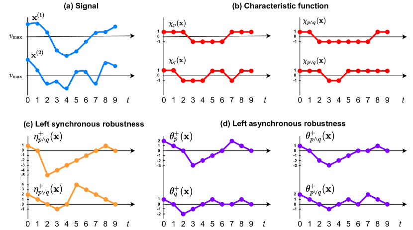
Figure 1. Evolution of the (a) signal, (b) characteristic function, (c) left synchronous temporal robustness and (d) left asynchronous temporal robustness from Example 1.

We first define the notion of left and right synchronous temporal robustness. The idea behind synchronous temporal robustness is to quantify the maximal amount of time by which we can shift the characteristic function $\chi_{\varphi}(\mathbf{x},t)$ of $\varphi$ to the left and right, respectively, without changing the value of $\chi_{\varphi}(\mathbf{x},t)$.

Definition 3.0 (Synchronous Temporal Robustness).

The left and right synchronous temporal robustness $\eta^{\pm}_{\varphi}(\mathbf{x},\!t):X^{\mathbb{T}}\!\times\!\mathbb{T}\!\to\!\overline{\mathbb{T}}$ of an STL formula $\varphi$ with respect to a signal $\mathbf{x}$ at time $t$ are defined as:

(2) $$\eta^{+}_{\varphi}(\mathbf{x},t) :=\chi_{\varphi}(\mathbf{x},t)\cdot\sup\{\tau\geq 0\ :\ \forall t^{\prime}\in[t,t+\tau],\ \chi_{\varphi}(\mathbf{x},t^{\prime})=\chi_{\varphi}(\mathbf{x},t)\}$$

(3) $$\eta^{-}_{\varphi}(\mathbf{x},t) :=\chi_{\varphi}(\mathbf{x},t)\cdot\sup\{\tau\geq 0\ :\ \forall t^{\prime}\in[t-\tau,t],\ \chi_{\varphi}(\mathbf{x},t^{\prime})=\chi_{\varphi}(\mathbf{x},t)\}.$$

For brevity, we often use the combined notation as follows:

$$\eta^{\pm}_{\varphi}(\mathbf{x},t):=\chi_{\varphi}(\mathbf{x},t)\cdot\sup\{\tau\geq 0\ :\ \forall t^{\prime}\in t\pm[0,\tau],\ \chi_{\varphi}(\mathbf{x},t^{\prime})=\chi_{\varphi}(\mathbf{x},t)\}.$$

Example 1.

Take a look at Fig. 1. The signal $\mathbf{x}:=[\mathbf{x}^{(1)},\,\mathbf{x}^{(2)}]$ presented in Fig.1(a) is finite and discrete-time, its state at each time step $t=0,\ldots,9$ is $x_{t}:=[x_{t}^{(1)},\,x_{t}^{(2)}]\in\mathbb{R}^{2}$. Let the two predicates be $p:=x^{(1)}_{t}\geq v_{\max}$ and $q:=x^{(2)}_{t}\geq v_{\max}$ for some given $v_{\max}$. The characteristic functions for the predicates $p$ and $q$ and the STL formulas $\varphi_{1}:=p\wedge q$ and $\varphi_{2}:=p\vee q$ are shown in Fig. 1(b). The evolution of the left synchronous temporal robustness $\eta^{+}_{\varphi}(\mathbf{x},t)$, $t=0,\ldots,9$ for the STL formulas $\varphi_{1}$ and $\varphi_{2}$ is presented in Fig. 1(c). For instance, consider the time point $t=0$ and the formula $\varphi_{2}$. Since $\chi_{\varphi_{2}}(\mathbf{x},0)=\chi_{\varphi_{2}}(\mathbf{x},1)=\chi_{\varphi_{2}}(\mathbf{x},2)=1$ and $\chi_{\varphi_{2}}(\mathbf{x},3)=-1$, then by Definition 3.1 it holds that $\eta^{+}_{\varphi_{2}}(\mathbf{x},0)=2$. On the other hand, for $\varphi_{1}$ and $t=6$, we have that $\chi_{\varphi_{1}}(\mathbf{x},6)=\chi_{\varphi_{1}}(\mathbf{x},7)=-1\not=1=\chi_{\varphi_{1}}(\mathbf{x},8)$ so that $\eta^{+}_{\varphi_{1}}(\mathbf{x},6)=-1$.

Some remarks are in place. Let $\mathbf{s}$ be a signal that is equivalent to $\mathbf{x}$ but shifted by $\tau$ time units to the left, i.e., $s_{t}:=x_{t+\tau}$ for all $t\in\mathbb{T}$. Then it holds that $\chi_{\varphi}(\mathbf{s},t)=\chi_{\varphi}(\mathbf{x},t+\tau)$. Similarly, $\chi_{\varphi}(\mathbf{s},t)=\chi_{\varphi}(\mathbf{x},t-\tau)$ where $\mathbf{s}$ is equivalent to $\mathbf{x}$ shifted by $\tau$ to the right, i.e., $s_{t}:=x_{t-\tau}$ for all $t\in\mathbb{T}$. This indicates, and is later formally shown in Section 5, that the left and right synchronous temporal robustness quantify the maximal amount of time by which we can synchronously shift the signal $\mathbf{x}$ (or alternatively each predicate in $\varphi$) to the left and right, respectively, without changing the value of $\chi_{\varphi}(\mathbf{x},t)$.

3.2. Asynchronous Temporal Robustness

While the synchronous temporal robustness quantifies the amount by which we can shift all predicates synchronously in time, the left and right asynchronous temporal robustness, which is inspired by (Donzé and Maler, 2010) and defined next, quantifies the maximal amount of time by which we can asynchronously shift individual predicates in $\varphi$ to the left and right, respectively.

Definition 3.0 (Asynchronous Temporal Robustness (inspired by (Donzé and Maler, 2010))).

The left and right asynchronous temporal robustness $\theta^{\pm}_{\varphi}(\mathbf{x},t):X^{\mathbb{T}}\times\mathbb{T}\to\overline{\mathbb{T}}$ of an STL formula $\varphi$ with respect to a signal $\mathbf{x}$ at time $t$ are defined recursively as:

(4) $$\theta^{+}_{p}(\mathbf{x},t):=\chi_{p}(\mathbf{x},t)\cdot\sup\{\tau\geq 0\ :\ \forall t^{\prime}\in[t,t+\tau],\ \chi_{p}(\mathbf{x},t^{\prime})=\chi_{p}(\mathbf{x},t)\}$$

(5) $$\theta^{-}_{p}(\mathbf{x},t):=\chi_{p}(\mathbf{x},t)\cdot\sup\{\tau\geq 0\ :\ \forall t^{\prime}\in[t-\tau,t],\ \chi_{p}(\mathbf{x},t^{\prime})=\chi_{p}(\mathbf{x},t)\}$$

and then applying to each $\theta^{\pm}_{p}(\mathbf{x},t)$ the recursive rules of the operators similarly to Definition. 2.1, which leads to:

(6) $$\theta^{\pm}_{\neg\varphi}(\mathbf{x},t) :=-\theta^{\pm}_{\varphi}(\mathbf{x},t)$$

(7) $$\theta^{\pm}_{\varphi_{1}\wedge\varphi_{2}}(\mathbf{x},t) :=\theta^{\pm}_{\varphi_{1}}(\mathbf{x},t)\ \sqcap\ \theta^{\pm}_{\varphi_{2}}(\mathbf{x},t)$$

(8) $$\theta^{\pm}_{\varphi_{1}\mathcal{U}_{I}\varphi_{2}}(\mathbf{x},t) :=\bigsqcup_{t^{\prime}\in t+I}\left(\theta^{\pm}_{\varphi_{2}}(\mathbf{x},t^{\prime})\ \sqcap\ \bigsqcap_{t^{\prime\prime}\in[t,t^{\prime})}\theta^{\pm}_{\varphi_{1}}(\mathbf{x},t^{\prime\prime})\right)$$

Remark 3.3.

There are two subtle difference between Definition 3.2 and temporal robustness in (Donzé and Maler, 2010, Definition 4). First, we use the supremum operator instead of the maximum operator in our definition. The benefit is that the supremum always exists. Second, compared with (Donzé and Maler, 2010, Definition 4), we use the characteristic function $\chi_{p}(\mathbf{x},t)$ of $p$ instead of the characteristic function $\chi_{\varphi}(\mathbf{x},t)$ of $\varphi$ in the definitions of $\theta^{+}_{p}(\mathbf{x},t)$ and $\theta^{-}_{p}(\mathbf{x},t)$ in (4) and (5), respectively.

Example 2 (continues=ex:running).

Take a look again at the signal $\mathbf{x}$ shown in Fig. 1. The evolution of the left asynchronous temporal robustness $\theta^{+}_{p}(\mathbf{x},t)$ , $\theta^{+}_{q}(\mathbf{x},t)$ , $\theta^{+}_{\varphi_{1}}(\mathbf{x},t)$ and $\theta^{+}_{\varphi_{2}}(\mathbf{x},t)$ is presented in Fig. 1(d). In order to estimate the left asynchronous temporal robustness for $\varphi_{1}=p\wedge q$ at time point $t$ over the given signal $\mathbf{x}$, one must first obtain the $\theta^{+}_{p}(\mathbf{x},t)$ and $\theta^{+}_{q}(\mathbf{x},t)$ values and then apply the conjunction rule (7). For instance, $\theta^{+}_{\varphi_{1}}(\mathbf{x},0):=\theta^{+}_{p}(\mathbf{x},0)\,\sqcap\,\theta^{+}_{q}(\mathbf{x},0)=1$. Analogously, one could obtain that for $\varphi_{2}=p\vee q$, the left asynchronous temporal robustness $\theta^{+}_{\varphi_{2}}(\mathbf{x},0):=\theta^{+}_{p}(\mathbf{x},0)\,\sqcup\,\theta^{+}_{q}(\mathbf{x},0)=2$.

Note that though the asynchronous temporal robustness $\theta^{\pm}_{\varphi}(\mathbf{x},t)$ is defined in a recursive manner, the synchronous temporal robustness $\eta^{\pm}_{\varphi}(\mathbf{x},t)$ does not follow the recursive rules.

4. Soundness of Temporal Robustness for Continuous-Time Signals

In this section, we provide soundness results that state the relationship between the synchronous and asynchronous temporal robustness and the Boolean semantics of STL. Section 4.1 presents the main results for synchronous temporal robustness, while Section 4.2 present analogous results for the asynchronous temporal robustness. While we provide our main results for continuous-time signals, we remark how the results simplify for discrete-time signals. The proofs of our technical results are provided in Appendix A.

4.1. Properties of Synchronous Temporal Robustness

The next theorem follows directly from Definition 3.1 and is fundamental to correctness of our solution to the control synthesis problem defined in Section 6.

Theorem 4.1 (Soundness).

For an STL formula $\varphi$, signal $\mathbf{x}:\mathbb{T}\rightarrow X$ and some time $t\in\mathbb{T}$, the following results hold:

1. $\eta^{\pm}_{\varphi}(\mathbf{x},t)>0\quad\,\Longrightarrow\ \chi_{\varphi}(\mathbf{x},t)=+1$

2. $\eta^{\pm}_{\varphi}(\mathbf{x},t)<0\quad\,\Longrightarrow\ \chi_{\varphi}(\mathbf{x},t)=-1$

3. $\chi_{\varphi}(\mathbf{x},t)=+1\ \Longrightarrow\ \eta^{\pm}_{\varphi}(\mathbf{x},t)\geq 0$

4. $\chi_{\varphi}(\mathbf{x},t)=-1\ \Longrightarrow\ \eta^{\pm}_{\varphi}(\mathbf{x},t)\leq 0$

To illustrate the previous result, let us again consider Example 1.

Example 3 (continues=ex:running).

Take again a look at Fig. 1 and consider the formula $\varphi_{2}=p\vee q$. From Fig. 1(c) one can see that $\eta^{+}_{\varphi_{2}}(\mathbf{x},0)=2>0$ so that, due to Theorem 4.1, $\chi_{\varphi}(\mathbf{x},0)=1$ has to hold, which can indeed be verified in Fig. 1(b). Note that the equivalence $\eta^{\pm}_{\varphi}(\mathbf{x},t)\geq 0\Longleftrightarrow\chi_{\varphi}(\mathbf{x},t)=1$ does not hold. In other words, when $\eta^{\pm}_{\varphi}(\mathbf{x},t)=0$, we can not determine if the formula is satisfied or violated. For instance, consider the time points $t=2$ and $t=4$ in Fig. 1 and note that $\eta^{+}_{\varphi_{2}}(\mathbf{x},2)=\eta^{+}_{\varphi_{2}}(\mathbf{x},4)=0$, but that $\chi_{\varphi_{2}}(\mathbf{x},2)=1$ and $\chi_{\varphi_{2}}(\mathbf{x},4)=-1$.

The next result follows directly from Theorem 4.1 and represents the connection between the left and the right synchronous temporal robustness.

Corollary 4.2.

For an STL formula $\varphi$, signal $\mathbf{x}:\mathbb{T}\rightarrow X$ and some time $t\in\mathbb{T}$, the following properties hold:

1. $\eta^{\pm}_{\varphi}(\mathbf{x},t)>0\quad\Longrightarrow\quad\eta^{\mp}_{\varphi}(\mathbf{x},t)\geq 0$.

2. $\eta^{\pm}_{\varphi}(\mathbf{x},t)<0\quad\Longrightarrow\quad\eta^{\mp}_{\varphi}(\mathbf{x},t)\leq 0$.

In this paper, we are interested in time shifts. As a first step, we next present a result towards understanding the connection between the synchronous temporal robustness $\eta^{\pm}_{\varphi}(\mathbf{x},t)$ and values of $\tau$ for which $\chi_{\varphi}(\mathbf{x},t)$ and $\chi_{\varphi}(\mathbf{x},t+\tau)$ are the same. This result establishes an equivalence between the left (right) synchronous temporal robustness and the maximum time in the future (past) without changing the satisfaction of the formula. While this gives a first interpretation of temporal robustness, we analyze temporal robustness in terms of synchronous and asynchronous time shifts in the signal $\mathbf{x}$ itself in detail in Section 5.

Theorem 4.3.

For an STL formula $\varphi$, signal $\mathbf{x}:\mathbb{R}\rightarrow X$, time $t\in\mathbb{R}$ and some value $r\in\overline{\mathbb{R}}_{\geq 0}$, the following result holds:

$$|\eta^{\pm}_{\varphi}(\mathbf{x},t)|=r\quad\Longleftrightarrow\quad \forall t^{\prime}\in t\pm[0,r),\ \chi_{\varphi}(\mathbf{x},t^{\prime})=\chi_{\varphi}(\mathbf{x},t)\qquad\text{and}$$

$$\text{if }r<\infty,\text{ then }\forall\epsilon>0,\ \exists\tau\in[r,r+\epsilon),\ \chi_{\varphi}(\mathbf{x},t\pm\tau)\not=\chi_{\varphi}(\mathbf{x},t).$$

The interpretation of Theorem 4.3 is as follows. Consider the case of finite left synchronous temporal robustness, i.e., $\eta^{+}_{\varphi}(\mathbf{x},t)=r<\infty$. Then for all times $t+[0,r)$, the formula satisfaction is the same, i.e., for all $t^{\prime}\in t+[0,r)$ we have that $\chi_{\varphi}(\mathbf{x},t^{\prime})=\chi_{\varphi}(\mathbf{x},t)$. Note that the interval $[0,r)$ is right-open and that we can not in general guarantee that $\chi_{\varphi}(\mathbf{x},t+r)=\chi_{\varphi}(\mathbf{x},t)$. We can, however, guarantee that in close proximity of $t+r$ (quantified by $\epsilon$ in Theorem 4.3) the satisfaction $\chi_{\varphi}(\mathbf{x},t^{\prime\prime})$ must change.

Note that the right-open interval $[0,r)$ and the existence of $\epsilon$ in Theorem 4.3 appears due to the $\sup$ operator in Definition 3.2 For discrete-time signals, the interval $[0,r)$ becomes closed and $\epsilon$ disappears. Particularly, for the special case of a discrete-time signal $\mathbf{x}:\mathbb{Z}\rightarrow X$ and if $\eta^{\pm}_{\varphi}(\mathbf{x},t)$ is finite, we remark that Theorem 4.3 can instead be stated as:

(9) $$|\eta^{\pm}_{\varphi}(\mathbf{x},t)|=r\quad\Longleftrightarrow \forall t^{\prime}\in t\pm[0,r],\ \chi_{\varphi}(\mathbf{x},t^{\prime})=\chi_{\varphi}(\mathbf{x},t)\qquad\text{and}$$

$$\chi_{\varphi}(\mathbf{x},t\pm(r+1))\not=\chi_{\varphi}(\mathbf{x},t).$$

The next result states that the synchronous temporal robustness $\eta^{\pm}_{\varphi}(\mathbf{x},t)$ is a piece-wise linear function with segments either increasing with slope 1 or decreasing with slope $-1$, depending on $\chi_{\varphi}(\mathbf{x},t)$ and on the left or right synchronous temporal robustness.

Theorem 4.4.

For an STL formula $\varphi$, signal $\mathbf{x}:\mathbb{R}\rightarrow X$, time $t\in\mathbb{R}$ and some value $r\in\overline{\mathbb{R}}_{\geq 0}$, the following result holds:

$$|\eta^{\pm}_{\varphi}(\mathbf{x},t)|=r\quad\Longrightarrow\quad\forall\tau\in[0,r),\ |\eta^{\pm}_{\varphi}(\mathbf{x},t\pm\tau)|=r-\tau.$$

For the special case of a discrete-time signal $\mathbf{x}:\mathbb{Z}\rightarrow X$ and if $\eta^{\pm}_{\varphi}(\mathbf{x},t)$ is finite, we remark that Theorem 4.4 can instead be stated as:

(10) $$|\eta^{\pm}_{\varphi}(\mathbf{x},t)|=r\quad\Longrightarrow\quad\forall\tau\in[0,r],\ |\eta^{\pm}_{\varphi}(\mathbf{x},t\pm\tau)|=r-\tau.$$

The above result can be interpreted in the sense that the absolute value of the synchronous temporal robustness decreases proportionally with the amount of time shift $\tau$. For instance, Fig. 1(c) shows how the function $\eta^{+}_{p\wedge q}(\mathbf{x},t)$ consists of the three linear segments:

$$\eta^{+}_{p\wedge q}(\mathbf{x},t)=\begin{cases}1-t,&\text{if}\ t\in\{0,1\}\\ t-7,&\text{if}\ t\in\{2,\ldots,7\}\\ 9-t,&\text{if}\ t\in\{8,9\}\end{cases}$$

4.2. Properties of Asynchronous Temporal Robustness

In this section, we provide similar soundness results for the asynchronous temporal robustness. Theorem 4.5 and Corollary 4.6, presented below, resemble Theorem 4.1 and Corollary 4.2 for the synchronous temporal robustness as one would expect. However, Theorems 4.7 and 4.8, also presented below, do not directly resemble the previous Theorems 4.3 and 4.4 due to the recursive nature of the definition for the asynchronous temporal robustness. For instance, in contrast to Theorem 4.3, Theorem 4.7 only states a sufficient condition. In Theorem 4.4, compared to Theorem 4.4, we can only provide a lower bound instead of an equality.

Theorem 4.5 (Soundness (Rodionova et al., 2021)).

For an STL formula $\varphi$, signal $\mathbf{x}:\mathbb{T}\rightarrow X$ and some time $t\in\mathbb{T}$, the following results hold:

1. $\theta^{\pm}_{\varphi}(\mathbf{x},t)>0\quad\,\Longrightarrow\ \chi_{\varphi}(\mathbf{x},t)=+1$

2. $\theta^{\pm}_{\varphi}(\mathbf{x},t)<0\quad\,\Longrightarrow\ \chi_{\varphi}(\mathbf{x},t)=-1$

3. $\chi_{\varphi}(\mathbf{x},t)=+1\ \Longrightarrow\ \theta^{\pm}_{\varphi}(\mathbf{x},t)\geq 0$

4. $\chi_{\varphi}(\mathbf{x},t)=-1\ \Longrightarrow\ \theta^{\pm}_{\varphi}(\mathbf{x},t)\leq 0$

Note that, again, the equivalence $\theta^{\pm}_{\varphi}(\mathbf{x},t)\geq 0\Longleftrightarrow\chi_{\varphi}(\mathbf{x},t)=+1$ does not hold. In other words, when $\theta^{\pm}_{\varphi}(\mathbf{x},t)=0$ we can not determine if the formula is satisfied or violated. The next result is a straightforward corollary from Theorem 4.5.

Corollary 4.6.

For an STL formula $\varphi$, signal $\mathbf{x}:\mathbb{T}\rightarrow X$ and some time $t\in\mathbb{T}$, the following results represent the connections between the left and the right asynchronous temporal robustness:

1. $\theta^{\pm}_{\varphi}(\mathbf{x},t)>0\quad\Longrightarrow\quad\theta^{\mp}_{\varphi}(\mathbf{x},t)\geq 0$.

2. $\theta^{\pm}_{\varphi}(\mathbf{x},t)<0\quad\Longrightarrow\quad\theta^{\mp}_{\varphi}(\mathbf{x},t)\leq 0$.

Similarly to the previous section and Theorem 4.3 that was stated for synchronous temporal robustness, we now analyze the connection between the asynchronous temporal robustness $\theta^{\pm}_{\varphi}(\mathbf{x},t)$ and values of $\tau$ for which $\chi_{\varphi}(\mathbf{x},t)$ and $\chi_{\varphi}(\mathbf{x},t+\tau)$ are the same.

Theorem 4.7.

For an STL formula $\varphi$, signal $\mathbf{x}:\mathbb{R}\rightarrow X$, time $t\in\mathbb{R}$ and some value $r\in\overline{\mathbb{R}}_{\geq 0}$, the following result holds:

$$|\theta^{\pm}_{\varphi}(\mathbf{x},t)|=r\quad\Longrightarrow\quad\forall t^{\prime}\in t\pm\,[0,r),\ \chi_{\varphi}(\mathbf{x},t^{\prime})=\chi_{\varphi}(\mathbf{x},t)$$

Note that Theorem 4.7 only provides a sufficient condition unlike Theorem 4.3. In other words, due to the recursive definition of the asynchronous temporal robustness, one can not guarantee the existence of the time shift that would change the formula satisfaction as in the second line of Theorem 4.3. For instance, in Fig. 1 one could get that $\theta^{+}_{p\vee q}(\mathbf{x},5)=1$ but $\chi_{p\vee q}(\mathbf{x},5)=...=\chi_{p\vee q}(\mathbf{x},9)=1$. For the special case of a discrete-time signal $\mathbf{x}:\mathbb{Z}\rightarrow X$ and if $\theta^{\pm}_{\varphi}(\mathbf{x},t)$ is finite, we remark that Theorem 4.7 can instead be stated as:

(11) $$|\theta^{\pm}_{\varphi}(\mathbf{x},t)|=r\quad\Longrightarrow\quad\forall t^{\prime}\in t\pm\,[0,r],\ \chi_{\varphi}(\mathbf{x},t^{\prime})=\chi_{\varphi}(\mathbf{x},t).$$

We next show how the asynchronous temporal robustness changes with time.

Theorem 4.8.

For an STL formula $\varphi$, signal $\mathbf{x}:\mathbb{R}\rightarrow X$, time $t\in\mathbb{R}$ and some value $r\in\overline{\mathbb{R}}_{\geq 0}$, the following result holds:

$$|\theta^{\pm}_{\varphi}(\mathbf{x},t)|=r\quad\Longrightarrow\quad\forall\tau\in[0,r),\ |\theta^{\pm}_{\varphi}(\mathbf{x},t\pm\tau)|\geq r-\tau.$$

Note that, compared to Theorem 4.4, no equality can be stated on the right side of the implication operator. One can not guarantee the steady increase or decrease of the asynchronous temporal robustness in time and obtain an exact value of the shifted temporal robustness. In fact, one can only provide a lower bound on its value. For the special case of a discrete-time signal $\mathbf{x}:\mathbb{Z}\rightarrow X$ and if $\theta^{\pm}_{\varphi}(\mathbf{x},t)$ is finite, we remark that Theorem 4.8 can instead be stated as:

(12) $$|\theta^{\pm}_{\varphi}(\mathbf{x},t)|=r\quad\Longrightarrow\quad\forall\tau\in[0,r],\ |\theta^{\pm}_{\varphi}(\mathbf{x},t\pm\tau)|\geq r-\tau.$$

4.3. The Relationship between Synchronous and Asynchronous Temporal Robustness

Until now we have not yet established the precise relationship between the two notions of temporal robustness and how they relate to each other. The properties specified in the previous Section 4 suggest some similarities and differences between these temporal robustness notions. For instance, it is easy to see from Definitions 3.1 and 3.2 that for the simple case of the specification $\varphi$ being a predicate $p$ the two notions are equal to each other.

Corollary 4.9.

$\theta^{\pm}_{p}(\mathbf{x},t)=\eta^{\pm}_{p}(\mathbf{x},t)$ for any $t\in\mathbb{T}$ and any $\mathbf{x}:\mathbb{T}\rightarrow X$.

The following theorem shows that the asynchronous temporal robustness is upper bounded by the synchronous temporal robustness value.

Theorem 4.10.

Given an STL formula $\varphi$ and a signal $\mathbf{x}:\mathbb{T}\rightarrow X$, then for any $t\in\mathbb{T}$, the following inequality holds:

$$|\theta^{\pm}_{\varphi}(\mathbf{x},t)|\leq|\eta^{\pm}_{\varphi}(\mathbf{x},t)|$$

Essentially, Theorem 4.10 states that the asynchronous temporal robustness is upper bounded by the synchronous temporal robustness. Together with the soundness Theorems 4.1 and 4.5, the following holds

$$\chi_{\varphi}(\mathbf{x},t)=+1\;\;\;\implies\;\;\;0\leq\theta^{\pm}_{\varphi}(\mathbf{x},t)\leq\eta^{\pm}_{\varphi}(\mathbf{x},t),$$

$$\chi_{\varphi}(\mathbf{x},t)=-1\;\;\;\implies\;\;\;\eta^{\pm}_{\varphi}(\mathbf{x},t)\leq\theta^{\pm}_{\varphi}(\mathbf{x},t)\leq 0.$$

As Example 1 suggests, the above inequalities are often strict. At this point, one may ask when equality holds. In fact there are fragments of STL for which equality indeed holds. These STL fragments include formulas in Negation Normal Form (Fainekos and Pappas, 2009b), i.e., negations only occur in front of predicates and the only other allowed operators are either the conjunction and always operators, denoted by $\varphi\in\text{STL}^{\!+}(\wedge,\square_{I})$, or the disjunction and eventually operators, denoted by $\varphi\in\text{STL}^{\!+}(\vee,\Diamond_{I})$. For the former STL fragment, the following holds.

Lemma 4.11.

Consider a formula $\varphi\in\text{STL}^{\!+}(\wedge,\square_{I})$ and a signal $\mathbf{x}:\mathbb{T}\rightarrow X$, then for any $t\in\mathbb{T}$ such that $\chi_{\varphi}(\mathbf{x},t)=1$ it follows that $\eta^{\pm}_{\varphi}(\mathbf{x},t)=\theta^{\pm}_{\varphi}(\mathbf{x},t)$.

For $\varphi\in\text{STL}^{\!+}(\vee,\Diamond_{I})$, we can obtain a similar result as follows.

Lemma 4.12.

Consider a formula $\varphi\in\text{STL}^{\!+}(\vee,\Diamond_{I})$ and a signal $\mathbf{x}:\mathbb{T}\rightarrow X$, then for any $t\in\mathbb{T}$ such that $\chi_{\varphi}(\mathbf{x},t)=-1$ it follows that $\eta^{\pm}_{\varphi}(\mathbf{x},t)=\theta^{\pm}_{\varphi}(\mathbf{x},t)$.

5. Robustness of Continuous-Time Signals with Respect to Time Shifts

So far, we have analyzed the connection between synchronous and asynchronous temporal robustness $\eta^{\pm}_{\varphi}(\mathbf{x},t)$ and $\theta^{\pm}_{\varphi}(\mathbf{x},t)$ and the satisfaction $\chi_{\varphi}(\mathbf{x},t)$ of an STL formula $\varphi$. In this section, we quantify the permissible synchronous and asynchronous time shifts in the signal $\mathbf{x}$ that do not lead to a change in the satisfaction of the formula. By Definition 2.1, the satisfaction $\chi_{\varphi}(\mathbf{x},t)$ of a formula $\varphi$ is recursively defined through the characteristic functions $\chi_{p_{k}}(\mathbf{x},t)$ of each predicate $p_{k}\in AP$ contained in $\varphi$. Therefore, from a satisfaction point of view, one could think about the permissible time shifts in terms of shifting the predicates via the characteristic function $\chi_{p_{k}}(\mathbf{x},t)$ in time, either synchronously (all $p_{k}$ together) or asynchronously (each $p_{k}$ independently).

5.1. Synchronous Temporal Robustness

We start with the properties of the synchronous temporal robustness and, therefore, first define the notion of synchronous $\tau$-early and synchronous $\tau$-late signals.

Definition 5.0 (Synchronously shifted early and late signals).

Let $\mathbf{x}\in X^{\mathbb{T}}$ be a signal, $AP$ be a given set of predicates and $\tau\in\mathbb{T}_{\geq 0}$. Then

• the signal $\mathbf{x}^{\leftarrow\tau}$ is called a synchronous $\tau$-early signal if

  (13) $$\forall p_{k}\in AP,\ \forall t\in\mathbb{T},\quad\chi_{p_{k}}(\mathbf{x}^{\leftarrow\tau},t)=\chi_{p_{k}}(\mathbf{x},t+\tau)$$

• the signal $\mathbf{x}^{\rightarrow\tau}$ is called a synchronous $\tau$-late signal if

  (14) $$\forall p_{k}\in AP,\ \forall t\in\mathbb{T},\quad\chi_{p_{k}}(\mathbf{x}^{\rightarrow\tau},t)=\chi_{p_{k}}(\mathbf{x},t-\tau)$$

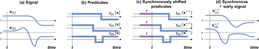
Figure 2. Synchronous $\tau$-early signal. (a) Signal $\mathbf{x}:=(\mathbf{x}_{(1)},\,\mathbf{x}_{(2)})$; (b) Evolution of the predicates $p_{1}:=\mathbf{x}_{(1)}\geq 0$, $p_{2}:=\mathbf{x}_{(2)}-\alpha\geq 0$ for given $\alpha>0$ and $p_{3}:=\mathbf{x}_{(2)}\geq 0$ over signal $\mathbf{x}$ through their characteristic function $\chi_{p_{k}}(\mathbf{x},t)$, $\forall t\in\mathbb{T}$, where $k\in\{1,2,3\}$; (c) Evolution of predicates $p_{1}$, $p_{2}$ and $p_{3}$ over signal $\mathbf{x}^{\leftarrow\tau}$ through their characteristic functions $\chi_{p_{k}}(\mathbf{x}^{\leftarrow\tau},t)$ which are equal to the characteristic functions $\chi_{p_{k}}(\mathbf{x},t)$ synchronously shifted to the left in time by $\tau$ for all $k\in\{1,2,3\}$ and $\forall t\in\mathbb{T}$; (d) Synchronous $\tau$-early signal $\mathbf{x}^{\leftarrow\tau}$.

Fig. 2 presents an example to illustrate the notion of a synchronous $\tau$-early signal. Fig. 2(a) depicts an initial signal $\mathbf{x}:=(\mathbf{x}_{(1)},\,\mathbf{x}_{(2)})$. Assume that the formula of interest $\varphi$ is built upon three predicates, i.e., $AP:=\{p_{1},p_{2},p_{3}\}$, where $p_{1}:=\mathbf{x}_{(1)}\geq 0$, $p_{2}:=\mathbf{x}_{(2)}-\alpha\geq 0$ and $p_{3}:=\mathbf{x}_{(2)}\geq 0$, for $\alpha>0$ as shown in Fig. 2(a) and (d). Fig. 2(b) shows the evolution of these three predicates $p_{1}$, $p_{2}$ and $p_{3}$ through their characteristic function $\chi_{p_{k}}(\mathbf{x},t)$ for all $t\in\mathbb{T}$ where $k\in\{1,2,3\}$. By synchronously shifting all three characteristic functions $\chi_{p_{k}}(\mathbf{x},t)$, $\forall t\in\mathbb{T}$ to the left by $\tau$ we obtain $\chi_{p_{k}}(\mathbf{x},t+\tau)$, $\forall t\in\mathbb{T}$, which are depicted in Fig. 2(c). Fig. 2(d) then shows a signal $\mathbf{x}^{\leftarrow\tau}$ that is a synchronous $\tau$-early signal due to (13) as the three synchronously shifted predicates in Fig. 2(c) correspond to the predicates of $\mathbf{x}^{\leftarrow\tau}$.

Remark 5.2.

If $\mathbf{s}$ is defined as $s_{t}:=x_{t\pm\tau}$, i.e., we shift the entire signal $\mathbf{x}$ by $\tau$, then it holds that $\forall p_{k}\in AP$ and $\forall t\in\mathbb{T}$ we have that $\chi_{p_{k}}(\mathbf{s},t)=\chi_{p_{k}}(\mathbf{x},t\pm\tau)$, i.e., $\mathbf{s}=\mathbf{x}^{\leftrightarrows\tau}$ is a synchronous $\tau$-early/late signal.

The next result follows by Definitions 2.1 and 5.1.

Corollary 5.3.

For an STL formula $\varphi$ built upon the predicate set $AP$, some $\tau\in\mathbb{T}_{\geq 0}$ and signal $\mathbf{x}:\mathbb{T}\rightarrow X$ it holds that $\forall t\in\mathbb{T}$,

$$\chi_{\varphi}(\mathbf{x}^{\leftrightarrows\tau},t)=\chi_{\varphi}(\mathbf{x},t\pm\tau).$$

Note that Corollary 5.3 is only a sufficient but not a necessary condition in the sense that there may exist signals $\mathbf{s}\not=\mathbf{x}^{\leftrightarrows\tau}$ for which $\chi_{\varphi}(\mathbf{s},t)=\chi_{\varphi}(\mathbf{x},t\pm\tau)$. For example, Fig.3(a) shows the characteristic function for the predicates $p$ and $q$ and the formula $p\vee q$ over a signal $\mathbf{x}$. Fig.3(b) shows the same functions but over another signal $\mathbf{s}$. One can see that $\forall t\in\mathbb{T}$, $\chi_{p\vee q}(\mathbf{s},t)=\chi_{p\vee q}(\mathbf{x},t+1)$ but $\mathbf{s}\not=\mathbf{x}^{\leftarrow 1}$. This is so because $\chi_{p}(\mathbf{s},t)=\chi_{p}(\mathbf{x},t)$ and $\chi_{q}(\mathbf{s},t)=\chi_{q}(\mathbf{x},t+2)$, therefore,  (13) is not satisfied.

We are now ready to state the main result that establishes a connection between the synchronous temporal robustness $\eta^{\pm}_{\varphi}(\mathbf{x},t)$ and the permissible time shifts $\tau$ via $\mathbf{x}^{\leftrightarrows{\tau}}$. We note, that the proofs of all technical results presented in this section are provided in Appendix B.

Figure 3. Predicates $p$ and $q$ and formula $p\vee q$ satisfaction over (a) signal $\mathbf{x}$ and (b) signal $\mathbf{s}$. One can see that $\forall t\in\mathbb{T}$, $\chi_{p\vee q}(\mathbf{s},t)=\chi_{p\vee q}(\mathbf{x},t+1)$ but $\mathbf{s}\not=\mathbf{x}^{\leftarrow 1}$.

Theorem 5.4.

Let $\varphi$ be an STL formula built upon the predicate set $AP$ and $\mathbf{x}:\mathbb{R}\rightarrow X$ be a signal. For any time $t\in\mathbb{R}$ and $r\in\overline{\mathbb{R}}_{\geq 0}$, it holds that:

$$|\eta^{\pm}_{\varphi}(\mathbf{x},t)|=r\quad\Longleftrightarrow\quad \forall\tau\in[0,r),\ \chi_{\varphi}(\mathbf{x}^{\leftrightarrows\tau},t)=\chi_{\varphi}(\mathbf{x},t)\qquad\text{and}$$

$$\text{if }r<\infty,\text{ then }\forall\epsilon>0,\ \exists\tau\in[r,r+\epsilon),\ \chi_{\varphi}(\mathbf{x}^{\leftrightarrows\tau},t)\not=\chi_{\varphi}(\mathbf{x},t).$$

Note particularly that the previous result closely resembles Theorem 4.3. For the special case of a discrete-time signal $\mathbf{x}:\mathbb{Z}\rightarrow X$ and if $\eta^{\pm}_{\varphi}(\mathbf{x},t)$ is finite, we remark that Theorem 5.4 can instead be stated as:

(15) $$|\eta^{\pm}_{\varphi}(\mathbf{x},t)|=r\quad\Longleftrightarrow \forall\tau\in[0,r],\ \chi_{\varphi}(\mathbf{x}^{\leftrightarrows\tau},t)=\chi_{\varphi}(\mathbf{x},t)\qquad\text{and}$$

$$\chi_{\varphi}(\mathbf{x}^{\leftrightarrows r+1},t)\not=\chi_{\varphi}(\mathbf{x},t).$$

5.2. Asynchronous Temporal Robustness

Let us now continue by analyzing the asynchronous temporal robustness and first define the notion of asynchronous $\bar{\tau}$-early and asynchronous $\bar{\tau}$-late signals.

Definition 5.0 (Asynchronously shifted signal).

Let $\mathbf{x}\in X^{\mathbb{T}}$ be a signal, $AP:=\{p_{1},\ldots,p_{L}\}$ be a given set of predicates and $\tau_{1},\ldots,\tau_{L}\in\mathbb{T}_{\geq 0}$. Denote $\bar{\tau}:=(\tau_{1},\ldots,\tau_{L})$. Then

• the signal $\mathbf{x}^{\leftarrow\bar{\tau}}$ is called an asynchronous $\bm{\bar{\tau}}$-early signal if

  (16) $$\forall p_{k}\in AP,\ \forall t\in\mathbb{T},\quad\chi_{p_{k}}(\mathbf{x}^{\leftarrow\bar{\tau}},t)=\chi_{p_{k}}(\mathbf{x},t+\tau_{k})$$

• the signal $\mathbf{x}^{\rightarrow\bar{\tau}}$ is called an asynchronous $\bm{\bar{\tau}}$-late signal if,

  (17) $$\forall p_{k}\in AP,\ \forall t\in\mathbb{T}\quad\chi_{p_{k}}(\mathbf{x}^{\rightarrow\bar{\tau}},t)=\chi_{p_{k}}(\mathbf{x},t-\tau_{k})$$

Fig. 4 presents an example to illustrate the notion of an asynchronous $\bar{\tau}$-early signal. Similar to Fig. 2, Fig. 4(a)-(b) show the evolution of a signal $\mathbf{x}$ and the same three predicates of interest over this signal, respectively. In Fig. 4(c) one can see each predicate $p_{k}$ being asynchronously shifted to the left by an individual $\tau_{k}$, where $k\in\{1,2,3\}$. Fig. 4(d) then shows a signal $\mathbf{x}^{\leftarrow\bar{\tau}}$ that is an asynchronous $\bar{\tau}$-early signal due to (16) as the three asynchronously shifted predicates in Fig. 4(c) correspond to the predicates of $\mathbf{x}^{\leftarrow\bar{\tau}}$.

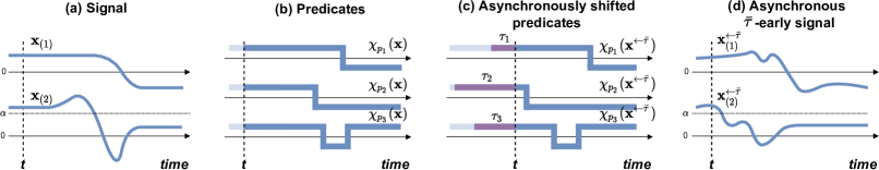
Figure 4. Asynchronous $\bar{\tau}$-early signal. (a) Signal $\mathbf{x}:=(\mathbf{x}_{(1)},\,\mathbf{x}_{(2)})$; (b) Evolution of the predicates $p_{1}:=\mathbf{x}_{(1)}\geq 0$, $p_{2}:=\mathbf{x}_{(2)}-\alpha\geq 0$ for given $\alpha>0$ and $p_{3}:=\mathbf{x}_{(2)}\geq 0$ over signal $\mathbf{x}$ through their characteristic function $\chi_{p_{k}}(\mathbf{x},t)$, $\forall t\in\mathbb{T}$, where $k\in\{1,2,3\}$; (c) Evolution of predicates $p_{1}$, $p_{2}$ and $p_{3}$ over the signal $\mathbf{x}^{\leftarrow\bar{\tau}}$, $\bar{\tau}:=(\tau_{1},\tau_{2},\tau_{3})$ through their characteristic functions $\chi_{p_{k}}(\mathbf{x}^{\leftarrow\bar{\tau}},t)$ which are equal to the characteristic functions $\chi_{p_{k}}(\mathbf{x},t)$ asynchronously shifted in time by $\tau_{k}$ for each $k\in\{1,2,3\}$ and $\forall t\in\mathbb{T}$; (d) Asynchronous $\bar{\tau}$-early signal $\mathbf{x}^{\leftarrow\bar{\tau}}$.

Note particularly that the above Definition 5.5 allows to shift the characteristic function $\chi_{p_{k}}(\mathbf{x},t+\tau_{k})$ of each predicate $p_{k}$ individually (and hence asynchronously) via $\tau_{k}$. This is in contrast to Definition 5.1 where we shift the characteristic function $\chi_{p_{k}}(\mathbf{x},t+\tau)$ of each predicate $p_{k}$ by the same amount (and hence synchronously) via $\tau$. We are now ready to state the main result that establishes a connection between the asynchronous temporal robustness $\theta^{\pm}_{\varphi}(\mathbf{x},t)$ and the permissible time shifts $\bar{\tau}$ in the predicates via $\mathbf{x}^{\leftrightarrows\bar{\tau}}$.

Theorem 5.6.

Let $\varphi$ be an STL formula built upon the predicate set $AP:=\{p_{1},\ldots,p_{L}\}$ and $\mathbf{x}:\mathbb{R}\rightarrow X$ be a signal. For any time $t\in\mathbb{R}$ and $r\in\overline{\mathbb{R}}_{\geq 0}$, it holds that:

$$|\theta^{\pm}_{\varphi}(\mathbf{x},t)|=r\quad\Longrightarrow\quad\forall\tau_{1},\ldots,\tau_{L}\in[0,r),\quad\chi_{\varphi}(\mathbf{x}^{\leftrightarrows\bar{\tau}},t)=\chi_{\varphi}(\mathbf{x},t)$$

where $\bar{\tau}:=(\tau_{1},\ldots,\tau_{L})$.

Note that Theorem 5.6 only provides a sufficient condition unlike Theorem 5.4. In other words, due to the recursive definition of the asynchronous temporal robustness, one can not guarantee the existence of the time shift that would change the formula satisfaction as in the second line of Theorem 5.4. For the special case of a discrete-time signal $\mathbf{x}:\mathbb{Z}\rightarrow X$ and if $\theta^{\pm}_{\varphi}(\mathbf{x},t)$ is finite, we remark that Theorem 5.6 can instead be stated as:

(18) $$|\theta^{\pm}_{\varphi}(\mathbf{x},t)|=r\quad\Longrightarrow\quad\forall\tau_{1},\ldots,\tau_{L}\in[0,r],\quad\chi_{\varphi}(\mathbf{x}^{\leftrightarrows\bar{\tau}},t)=\chi_{\varphi}(\mathbf{x},t).$$

The definitions of asynchronous $\bar{\tau}$-early and asynchronous $\bar{\tau}$-late signals together with Theorem 5.6 quantify the permissible time shift $\bar{\tau}$ in terms of how much each predicate $p_{k}$ in $\varphi$ can be shifted via the characteristic function $\chi_{p_{k}}(\mathbf{x},t\pm\tau_{k})$. Let us next analyze under which conditions these time shifts directly correlate with time shifts in the underlying signal $\mathbf{x}$. Consider a signal $\mathbf{x}:\mathbb{T}\rightarrow X$ with its state $x_{t}:=(x^{(1)}_{t}\ldots,x^{(n)}_{t})\in\mathbb{R}^{n}$. We will use $\kappa$ to denote time shifts in the elements of $x_{t}$, in contrast to $\tau$ for the time shifts in the predicates. First, note that if all elements $x^{(i)}_{i}$ of the signal $\mathbf{x}$ are shifted in time by the same amount $\kappa$, i.e., $s^{(i)}_{t}:=x^{(i)}_{t\pm\kappa}$, $\forall i\in\{1,\ldots,n\}$, then due to Remark 5.2 we have that $\mathbf{s}$ is an asynchronous $\bar{\tau}$-early/late signal, i.e., $\mathbf{s}=\mathbf{x}^{\leftrightarrows\bar{\tau}}$ for $\bar{\tau}=(\kappa,\ldots,\kappa)$. In contrast, if time shifts are different across different elements of the state, the following may apply.

Remark 5.7.

If the signal $\mathbf{s}$ is defined as $s_{t}:=(x^{(1)}_{t\pm\kappa_{1}},\ldots,x^{(n)}_{t\pm\kappa_{n}})$, i.e., each element $x_{t}^{(i)}$ of $x_{t}$ is shifted individually by $\kappa_{i}$, then there might not exist any $\bar{\tau}:=(\tau_{1},\ldots,\tau_{L})$ such that $\mathbf{s}=\mathbf{x}^{\leftrightarrows\bar{\tau}}$. In other words, the signal $\mathbf{s}$ might not be an asynchronous $\bar{\tau}$-early/late signal.

Next we consider a specific example that will help us understand under what conditions asynchronously shifting the elements of the state in time leads to asynchronous early or late signals.

Example 4.

Consider three drones which are, for simplicity, assumed to only move in vertical direction. The state of each drone $d$ is $x^{(d)}:=(z^{(d)},v^{(d)})\in\mathbb{R}^{2}$ and comprises of altitude and velocity. We define the signal state as $x:=(x^{(1)},x^{(2)},x^{(3)})\in\mathbb{R}^{6}$. Assume that we allow time shifts only across the full state of each drone $x^{(d)}$, i.e., different drones can be shifted in time differently, but the altitude and velocity of each drone $d$ is shifted in time by the same amount $\kappa_{d}$. Formally, such shifted signal $\mathbf{s}$ can be defined as following:

$$s_{t}:=(s^{(1)}_{t},\,s^{(2)}_{t},\,s^{(3)}_{t})=(x^{(1)}_{t+\kappa_{1}},\,x^{(2)}_{t+\kappa_{2}},\,x^{(3)}_{t+\kappa_{3}}).$$

Also assume that predicates are defined over separate drones only. In this case, any predicate $p_{k}\in AP:=\{p_{1},\ldots,p_{L}\}$ that is defined over a drone $d$ can be represented as $\mu_{k}(x_{t}):=\nu_{k}(x^{(d)}_{t})$, where $\nu_{k}$ is some real-valued function. Therefore, the following holds for the predicate $p_{k}$:

$$\chi_{p_{k}}(\mathbf{s},t)\overset{\text{def}~{}\ref{def:char_func}}{:=}\operatorname{sign}\mu_{k}(s_{t})= \operatorname{sign}\nu_{k}(s^{(d)}_{t})$$

$$= \operatorname{sign}\nu_{k}(x^{(d)}_{t+\kappa_{i}})=\operatorname{sign}\mu_{k}(x_{t+\kappa_{d}})=\chi_{p_{k}}(\mathbf{x},t+\kappa_{d}).$$

Consequently, it holds that $\mathbf{s}=\mathbf{x}^{\leftarrow\bar{\tau}}$ where $\bar{\tau}=(\tau_{1},\ldots,\tau_{L})$ and each $\tau_{k}\in\{\kappa_{1},\kappa_{2},\kappa_{3}\}$. By applying Theorem 5.6, we can conclude that $\forall\kappa_{1},\kappa_{2},\kappa_{3}\in[0,r)$ it holds that $\chi_{\varphi}(\mathbf{s},t)=\chi_{\varphi}(\mathbf{x},t)$ if $|\theta^{+}_{\varphi}(\mathbf{x},t)|=r$. This means that, as long as within each drone the elements of the state are shifted in time dy the same amount, different drones can be shifted in time by the different amounts up to $|\theta^{+}_{\varphi}(\mathbf{x},t)|$, while formula satisfaction will not change.

We now formally state the result that establishes when asynchronously shifting the elements of the state in time leads to asynchronous early or late signals. Let us therefore consider that the signal $\mathbf{x}$ is defined as $x_{t}:=(\zeta^{(1)}_{t},\ldots,\zeta^{(c)}_{t})$ where $c$ the number of groups in which $x_{t}$ is clustered. For $d\in\{1,\ldots,c\}$, let us define the state as $\zeta^{(d)}_{t}:=(x^{(d_{1})}_{t},\ldots,x^{(d_{m})}_{t})$ for dimensions $d_{1},\ldots,d_{m}$.

Lemma 5.8.

Assume that every predicate $p_{k}\in AP:=\{p_{1},\ldots,p_{L}\}$ in $\varphi$ is defined over only a single $\zeta^{(d)}$ for some $d$ i.e., $\exists d\in\{1,\ldots,c\}$ and a real-valued function $\nu_{k}$, such that $p_{k}:=\nu_{k}(\zeta^{(d)}_{t})\geq 0$. If $\mathbf{s}$ is defined as $s_{t}:=(\zeta^{(1)}_{t\pm\kappa_{1}},\ldots,\zeta^{(c)}_{t\pm\kappa_{c}})$, i.e. each $\zeta^{(d)}$ is shifted by a different amount $\kappa_{d}$, then $\mathbf{s}=\mathbf{x}^{\leftrightarrows\bar{\tau}}$, i.e., $\mathbf{s}$ is an asynchronous $\bar{\tau}$ early/late signal, where $\bar{\tau}:=(\tau_{1},\ldots,\tau_{L})$ and each $\tau_{k}\in\{\kappa_{1},\ldots,\kappa_{c}\}$.

6. Temporally-Robust STL Control Synthesis

As mentioned before, in time-critical systems one is not only interested in satisfying an STL formula, but also in satisfying the formula robustly in terms of temporal robustness. In this section, our goal is to design control laws that maximize the temporal robustness of a dynamical system. We refer to this problem as the temporally-robust control synthesis problem and consider in the remainder discrete-time dynamical systems.

6.1. Problem Formulation

Consider a discrete-time, linear control system

(19) $$x_{t+1}:=Ax_{t}+Bu_{t},\;\;\;x_{0}\in X_{0}$$

where $x_{t}\in X\subseteq\mathbb{R}^{n}$ and $u_{t}\in U\subseteq\mathbb{R}^{m}$ are the state and control input of a linear dynamical system, respectively, where $X$ and $U$ are the workspace and the set of permissible control inputs. We assume that sets $X$ and $U$ can be represented as a set of MILP constraints, e.g., when $X$ and $U$ are polytopes. Let the system have an initial condition $x_{0}$ from the set $X_{0}$. Let $A$ and $B$ be the system matrices of appropriate dimensions. Before defining the temporally-robust control synthesis problem, we make two assumptions on the STL formula $\varphi$. First, we assume that $\varphi$ is built from linear predicate function, i.e., $\mu(x_{t})$ is a linear function of the state. Second, we assume that $\varphi$ is bounded-time with formula length $\textit{len}(\varphi)$. For the definition of the formula length, we refer the reader to (Raman et al., 2014).

Problem 1 (Temporally-Robust Control Synthesis).

Given an STL specification $\varphi$, a temporal robustness of interest $\vartheta\in\{\theta^{+}_{\varphi},\theta^{-}_{\varphi},\eta^{+}_{\varphi},\eta^{-}_{\varphi}\}$, a time horizon $H\geq\text{len}(\varphi)$, a discrete-time control system as in (19), and a desired lower bound $\vartheta^{*}>0$ on the temporal robustness $\vartheta$, solve

(20) $$\mathbf{u}^{*}= \underset{\mathbf{u}:=(u_{0},\ldots,u_{H-1})}{\text{argmax}}\quad\vartheta(\mathbf{x},0)$$

s.t. $$\quad x_{t+1}:=Ax_{t}+Bu_{t},\quad t=0,\ldots,H-1$$

$$\quad u_{t}\in U,\quad t=0,\ldots,H-1$$

$$\quad x_{t}\in X,\quad t=0,\ldots,H$$

$$\quad\vartheta(\mathbf{x},0)\geq\vartheta^{*}>0$$

Problem 1 aims at finding an optimal control sequence $\mathbf{u}^{*}$ such that the corresponding signal $\mathbf{x}$ not only respects the dynamics and input-state constraints presented by $X$ and $U$, but also robustly satisfies the given specification $\varphi$. Note that the last constraint in (20) particularly implies that the formula $\varphi$ is satisfied because we require the temporal robustness value to be strictly positive, see Theorems 4.1 and 4.5. Moreover, one can also control the desired lower bound $\vartheta^{*}$ on the temporal robustness that must be achieved by the system.

Solving Problem 1 poses several challenges as both the synchronous as well as the asynchronous temporal robustness are neither continuous nor smooth functions. Particularly the counting of time shifts, as expressed by the $\sup$ operator in the Definitions 3.1 and 3.2, does not allow for the use of the variety of existing methods for control under STL specifications, e.g., gradient-based solutions and smooth approximations as in (Pant et al., 2017) and (Abbas and Fainekos, 2013). This motivates the use of Mixed-Integer Linear Programming (MILP) to explicitly encode and solve Problem 1. In the remainder, we present an MILP encoding for the left temporal robustness and we remark that the right temporal robustness can be encoded analogously with only minor modifications, and is hence omitted.

Remark 6.1.

We note that Problem 1 can be encoded as an MILP for an even broader class of dynamical systems than in (19). As long as the system dynamics can be expressed as a set of MILP constraints, the overall encoding will lead to an MILP formulation. Such systems include, for instance, hybrid systems such as mixed logical dynamical systems (Bemporad and Morari, 1999), piecewise affine systems (Sontag, 1981), linear complementarity systems (van der Schaft and Schumacher, 1998), and max-min-plus-scaling systems (De Schutter and Van den Boom, 2000).

6.2. MILP Encoding of Synchronous Temporal Robustness

For the case of a finite left synchronous temporal robustness $\eta^{+}_{\varphi}(\mathbf{x},t)$, e.g., when considering a finite time horizon $H$ as in Problem 1, the $\sup$ operator in Definition 3.1 can be replaced by a $\max$ operator, i.e., we have that

(21) $$\eta^{+}_{\varphi}(\mathbf{x},t):=\chi_{\varphi}(\mathbf{x},t)\cdot\max\{\tau\geq 0\ :\ \forall t^{\prime}\in[t,t+\tau],\ \chi_{\varphi}(\mathbf{x},t^{\prime})=\chi_{\varphi}(\mathbf{x},t)\}.\\$$

Note that the calculation of $\eta^{+}_{\varphi}(\mathbf{x},t)$ is based on the characteristic function $\chi_{\varphi}(\mathbf{x},t)$. Therefore, we start our MILP encoding of the synchronous temporal robustness $\eta^{+}_{\varphi}(\mathbf{x},t)$ with the encoding of the STL formula $\varphi$ followed by the encoding of the $\max$ operator in (21).

Boolean encoding of STL constraints

Consider a binary variable $z^{\varphi}_{t}\in\{0,1\}$ that corresponds to the satisfaction of the formula $\varphi$ by the signal $\mathbf{x}$ at time point $t$, i.e. we let

(22) $$z_{t}^{\varphi}:=\begin{cases}1&\text{if}\ \chi_{\varphi}(\mathbf{x},t)=1\\ 0&\text{if}\ \chi_{\varphi}(\mathbf{x},t)=-1.\\ \end{cases}$$

In (Raman et al., 2014), a recursive MILP encoding of the variable $z_{t}^{\varphi}$ has been presented such that exactly the above relationship holds. We use this set of MILP constraints in the remainder to obtain an MILP encoding for the left synchronous temporal robustness $\eta^{+}_{\varphi}(\mathbf{x},t)$.

Encoding of the left synchronous temporal robustness

Using (22), the definition of the left temporal robustness $\eta^{+}_{\varphi}(\mathbf{x},t)$ in (21) can be written in terms of $z_{t}^{\varphi}$ as following:

(23) $$\eta^{+}_{\varphi}(\mathbf{x},t):=\begin{cases}\quad\max\{\tau\geq 0\ :\ \forall t^{\prime}\in[t,t+\tau],\ z_{t^{\prime}}^{\varphi}=1\}&\text{if}\ z_{t}^{\varphi}=1\\ -\max\{\tau\geq 0\ :\ \forall t^{\prime}\in[t,t+\tau],\ z_{t^{\prime}}^{\varphi}=0\}&\text{if}\ z_{t}^{\varphi}=0\end{cases}$$

In other words, if $z_{t}^{\varphi}=1$ one has to count the maximum number of sequential time points $t^{\prime}>t$ in the future for which $z_{t^{\prime}}^{\varphi}=1$. If $z_{t}^{\varphi}=0$, one has to count the maximum number of sequential time points $t^{\prime}>t$ in the future for which $z_{t^{\prime}}^{\varphi}=0$, and then multiply this number with $-1$. To implement this idea, we first construct the counter variable $c^{1,\varphi}_{t}\in\mathbb{Z}_{\geq 0}$ that counts sequential $z_{t^{\prime}}^{\varphi}=1$ for $t^{\prime}\geq t$. We also construct the second counter variable $c^{0,\varphi}_{t}\in\mathbb{Z}_{\geq 0}$ that counts the number of sequential $z_{t^{\prime}}^{\varphi}=0$ for $t^{\prime}\geq t$ and then multiplies the counted value by $-1$. Since we count steps into the future from $t$, we do this recursively and backwards in time as follows:

(24) $$c^{1,\varphi}_{t}:=(c^{1,\varphi}_{t+1}+1)\cdot z^{\varphi}_{t},\qquad\ \,\qquad c^{1,\varphi}_{H+1}:=0,$$

(25) $$c^{0,\varphi}_{t}:=(c^{0,\varphi}_{t+1}-1)\cdot(1-z^{\varphi}_{t}),\qquad c^{0,\varphi}_{H+1}:=0.$$

Note that temporal robustness is defined by $z^{\varphi}_{t^{\prime}}$ for which $t^{\prime}>t$ rather than $t^{\prime}\geq t$. Therefore, the previously defined counters $c^{1,\varphi}_{t}$, $c^{0,\varphi}_{t}$ must be adjusted by the value of 1 as follows:

(26) $$\tilde{c}^{1,\varphi}_{t}:=c^{1,\varphi}_{t}-z^{\varphi}_{t},$$

(27) $$\tilde{c}^{0,\varphi}_{t}:=c^{0,\varphi}_{t}+(1-z^{\varphi}_{t}).$$

Since the two cases in (23) are disjoint or, in other words, $z_{t}^{\varphi}$ is either $1$ or $0$, the overall left synchronous temporal robustness $\eta^{+}_{\varphi}(\mathbf{x},t)$ can be implemented as a sum of the two adjusted counters:

(28) $$\eta^{+}_{\varphi}(\mathbf{x},t):=\tilde{c}^{1,\varphi}_{t}+\tilde{c}^{0,\varphi}_{t}$$

Remark 6.2.

The constraints (24) and (25) contain a product of an integer variable with a Boolean variable. Such product can be expressed as a set of MILP constraints following Lemma D.2.

Input: Specification $\varphi$, signal $\mathbf{x}$.

Output: The left synchronous temporal robustness $\bm{\eta}^{+}_{\varphi}(\mathbf{x})$, the set of MILP constraints $\mathcal{H}$.

1: Let $z^{\varphi}_{t}\in\mathbb{B}$ be constrained by (22), where $t=0,\ldots,H$.

2: Let $c^{1,\varphi}_{t},c^{0,\varphi}_{t}\in\mathbb{Z}$ be constrained by (24) and (25), where $t=0,\ldots,H+1$.

3: Let $\tilde{c}^{1,\varphi}_{t},\tilde{c}^{0,\varphi}_{t}\in\mathbb{Z}$ be constrained by (26) and (27), where $t=0,\ldots,H$.

4: $\eta^{+}_{\varphi}(\mathbf{x},t)\overset{\eqref{eq:milp_eta_final}}{:=}\tilde{c}^{1,\varphi}_{t}+\tilde{c}^{0,\varphi}_{t}$, where $t=0,\ldots,H$.

5: $\mathcal{H}$ consists of the MILP constraints (22), (24), (25), (26), (27) and (28).

Algorithm 1 The function $(\bm{\eta}^{+}_{\varphi}(\mathbf{x}),\,\mathcal{H}):=\texttt{MILP\_SYNC}(\varphi,\mathbf{x})$

Table 1. Estimation of $\eta^{+}_{\varphi}(\mathbf{x},t)$ for $\varphi:=p\wedge q$ from Example 1 following Alg. 1.

$t$	0	1	2	3	4	5	6	7	8	9	10
$\chi_{\varphi}(\mathbf{x},t)$	1	1	-1	-1	-1	-1	-1	-1	1	1
$z_{t}^{\varphi}$, see (22)	1	1	0	0	0	0	0	0	1	1
$c^{1,\varphi}_{t}:=(c^{1,\varphi}_{t+1}+1)\cdot z^{\varphi}_{t}$, $\quad c^{1,\varphi}_{H+1}:=0$	2	1	0	0	0	0	0	0	2	1	0
$c^{0,\varphi}_{t}:=(c^{0,\varphi}_{t+1}-1)\cdot(1-z^{\varphi}_{t})$, $\quad c^{0,\varphi}_{H+1}:=0$	0	0	-6	-5	-4	-3	-2	-1	0	0	0
$\tilde{c}^{1,\varphi}_{t}:=c^{1,\varphi}_{t}-z^{\varphi}_{t}$	1	0	0	0	0	0	0	0	1	0
$\tilde{c}^{0,\varphi}_{t}:=c^{0,\varphi}_{t}+(1-z^{\varphi}_{t})$	0	0	-5	-4	-3	-2	-1	0	0	0
$\eta^{+}_{\varphi}(\mathbf{x},t):=\tilde{c}^{1,\varphi}_{t}+\tilde{c}^{0,\varphi}_{t}$	1	0	-5	-4	-3	-2	-1	0	1	0

The MILP encoding (22)-(28) of the left synchronous temporal robustness $\eta^{+}_{\varphi}(\mathbf{x},t)$ is formally summarized in Alg. 1. It outputs a set of MILP constraints $\mathcal{H}$ and $\eta^{+}_{\varphi}(\mathbf{x},t)$ for all time steps $t=0,\ldots,H$, denoted as $\bm{\eta}^{+}_{\varphi}(\mathbf{x})$. We summarize the main properties of the above MILP encoding in the following Proposition 6.1, while the proof is available in Appendix C.

Proposition 6.1.

Let $\mathbf{x}$ be a signal satisfying the recursion of the discrete-time dynamical system (19) and let $\varphi$ be an STL specification that is built upon linear predicates. Then:

1. The left synchronous temporal robustness sequence $\bm{\eta}^{+}_{\varphi}(\mathbf{x}):=(\eta^{+}_{\varphi}(\mathbf{x},0),\ldots,\eta^{+}_{\varphi}(\mathbf{x},H))$, with $\eta^{+}_{\varphi}(\mathbf{x},t)$ as in (21) is equivalent to the output $(\bm{\eta}^{+}_{\varphi}(\mathbf{x}),\,\mathcal{H}):=\texttt{MILP\_SYNC}(\varphi,\mathbf{x})$ of Alg. 1.

2. The MILP encoding of $\bm{\eta}^{+}_{\varphi}(\mathbf{x})$ in Alg. 1 is a function of $O(H\cdot|AP|)$ binary and $O(H\cdot|\varphi|)$ continuous variables, where $H$ is the time horizon, $|\varphi|$ is the number of operators in the formula $\varphi$, and $|AP|$ is the number of used predicates.

Example 5 (continues=ex:running).

Take a look again at the signal $\mathbf{x}$ and an STL formula $\varphi=p\wedge q$ evaluation shown in Fig. 1. In Table 1 we consider a step-by-step estimation of the left synchronous temporal robustness $\bm{\eta}^{+}_{\varphi}(\mathbf{x})$ following the MILP encoding procedure described above in Section 6.2 and formally defined in Alg. 1. From Figure 1(b) one can see that $\bm{\chi}_{p\wedge q}(\mathbf{x})=(1,1,-1,-1,-1,-1,-1,-1,1,1)$. Then following Alg. 1, one can see that $\bm{\eta}^{+}_{\varphi}(\mathbf{x})$ sequence is indeed equal to $(1,0,-5,-4,-3,-2,-1,0,1,0)$ shown in Fig. 1(c). Therefore, the MILP encoding procedure leads to the same result as its estimation by the definition.

Finally, using the MILP encoding of the left synchronous temporal robustness $\eta^{+}_{\varphi}(\mathbf{x},t)$ presented in Alg. 1, we summarize the overall MILP encoding of Problem 1 in case of $\vartheta=\eta^{+}_{\varphi}$ in Alg. 2. The function $\texttt{SYSTEM\_CONSTRAINTS}(x_{0},\mathbf{u})$ defines linear constraints on the decision variable $u_{t}$ according to (19) and such that $x_{t}\in X$. The below Proposition 6.2 states the correctness of our encoding and follows directly from the definition of Problem 1.

Proposition 6.2.

The temporally-robust STL control synthesis problem as defined in Problem 1 with synchronous left temporal robustness, i.e., $\vartheta=\eta^{+}_{\varphi}$, is equivalent to an MILP as described in Alg. 2.

We again remark that the case of synchronous right temporal robustness $\vartheta=\eta^{-}_{\varphi}$ can be handled almost identically.

Input: Specification $\varphi$, initial state $x_{0}$, time horizon $H$, minimum synchronous temporal robustness $\eta^{*}$

Output: Control input sequence $\mathbf{u}^{*}=(u^{*}_{0},\ldots,u^{*}_{H-1})$

Set $\mathbf{u}=(u_{0},\ldots,u_{H-1})$ to be the decision variable

$\,\mathbf{u}^{*}=\underset{\mathbf{u}}{\text{argmax}}\quad\eta^{+}_{\varphi}(\mathbf{x},0)$

$\qquad\quad\ \text{s.t.}\quad\ \ \,\eta^{+}_{\varphi}(\mathbf{x},0)\geq\eta^{*}>0$

$\qquad\qquad\qquad\ \,\mathbf{x}:=\texttt{SYSTEM\_CONSTRAINTS}(x_{0},\mathbf{u})$

$\qquad\qquad\qquad\ \,(\bm{\eta}^{+}_{\varphi}(\mathbf{x}),\,\mathcal{H}):=\texttt{MILP\_SYNC}(\varphi,\mathbf{x})$ // Sec. 6.2, Alg. 1

$\qquad\qquad\qquad\ \,\mathcal{H},\ u_{t}\in U$ for $t=0,\ldots,H-1$

Algorithm 2 MILP encoding of Problem 1 with the left synchronous temporal robustness objective $\vartheta:=\eta^{+}_{\varphi}$

6.3. MILP Encoding of Asynchronous Temporal Robustness

Recall that the left asynchronous temporal robustness $\theta^{+}_{\varphi}(\mathbf{x},t)$ from Definition 3.2 is defined recursively on the structure of $\varphi$. In contrast to the MILP encoding for the synchronous temporal robustness $\eta^{+}_{p}(\mathbf{x},t)$, we hence encode the left asynchronous temporal robustness $\theta^{+}_{p}(\mathbf{x},t)$ for every predicate $p$ containing in $\varphi$ first, and then encode the recursive rules (6)-(8) that are applied to every $\theta^{+}_{p}(\mathbf{x},t)$.

Encoding of STL predicates

Note that due to Corollary 4.9, $\theta^{\pm}_{p}(\mathbf{x},t)=\eta^{\pm}_{p}(\mathbf{x},t)$ for any $t\in\mathbb{T}$. Therefore, the MILP encoding of $\theta^{+}_{p}(\mathbf{x})$ is defined by the function $\texttt{MILP\_SYNC}(p,\mathbf{x})$ described by Alg. 1. Therefore, we can already summarize the encoding of STL predicates using MILP in the following corollary.

Corollary 6.3.

For a signal $\mathbf{x}$ satisfying the recursion of the discrete-time dynamical system (19) and a linear predicate $p\in AP$, the left asynchronous temporal robustness sequence $\bm{\theta}^{+}_{p}(\mathbf{x}):=(\theta^{+}_{p}(\mathbf{x},0),\ldots,\theta^{+}_{p}(\mathbf{x},H))$ with $\theta^{+}_{p}(\mathbf{x},t)$ defined by (4) is equivalent to the set of MILP constraints produced by the function $(\theta^{+}_{p}(\mathbf{x}),\,\mathcal{P}):=\texttt{MILP\_SYNC}(p,\mathbf{x})$ presented in Alg. 1.

Encoding of STL operators

Having encoded the temporal robustness of STL predicates as MILP constraints, the generalization to STL formulas is straight-forward and can use the encoding from (Raman et al., 2014). For example, let $\varphi=\wedge_{j=1}^{m}\varphi_{i}$ and $\theta^{+}_{\varphi_{j}}(\mathbf{x},t)=r_{j}$. By Definition 3.2 and following (7), we have that $\theta^{+}_{\varphi}(\mathbf{x},t)=\min_{j=1,\ldots,m}\theta^{+}_{\varphi_{j}}(\mathbf{x},t)$. Then $\theta^{+}_{\varphi}(\mathbf{x},t)=r$ if and only if the following MILP constraints hold:

(29) $$r_{j}-M(1-b_{j})\leq r\leq r_{j},\quad j=1,\ldots m$$

$$\sum_{j=1}^{m}b_{j}=1$$

where $b_{j}=\{0,1\}$ are introduced binary variables for $j=1,\ldots,m$ and $M$ is a big-$M$ parameter.

Input: Specification $\varphi$, signal $\mathbf{x}$

Output: The left asynchronous temporal robustness $\bm{\theta}^{+}_{\varphi}(\mathbf{x})$, set of MILP constraints $\mathcal{Q}$.

for $k=1,\ldots,L$ do

      

      $(\bm{\theta}^{+}_{p_{k}}(\mathbf{x}),\mathcal{P}_{k}):=\texttt{MILP\_SYNC}(p_{k},\mathbf{x})$ // Alg. 1

end for

$(\bm{\theta}^{+}_{\varphi}(\mathbf{x}),\mathcal{O}):=\texttt{MILP\_OPERATORS}(\varphi,\mathbf{x},\bm{\theta}^{+}_{p}(\mathbf{x}))$

$\mathcal{Q}:=\mathcal{O}\cup\bigcup_{k=1}^{L}\mathcal{P}_{k}$

Algorithm 3 The function $(\bm{\theta}^{+}_{\varphi}(\mathbf{x}),\,\mathcal{Q}):=\texttt{MIPL\_ASYN}(\varphi,\mathbf{x})$

The complete MILP encoding of the left asynchronous temporal robustness $\theta^{+}_{\varphi}(\mathbf{x},t)$ is formally summarized in Alg. 3, which consists of two steps. First, the encoding of the STL predicates, defined formally through the function $\texttt{MILP\_SYNC}(p_{k},\mathbf{x})$ for each predicate $p_{k}$ within $\varphi$. And second, the encoding of STL operators, defined through the function $\texttt{MILP\_OPERATORS}(\varphi,\mathbf{x},\bm{\theta}^{+}_{p}(\mathbf{x}))$ that is defined according to (Raman et al., 2014) and recursively follows the structure of $\varphi$. Alg. 3 outputs a set of MILP constraints $\mathcal{Q}$ and $\theta^{+}_{\varphi}(\mathbf{x},t)$ for all time steps $t=0,\ldots,H$, denoted as $\bm{\theta}^{+}_{\varphi}(\mathbf{x})$. We summarize the main properties of the above MILP formulation of the left asynchronous temporal robustness in Proposition 6.3, while the proof is available in Appendix C.

Proposition 6.3.

Let $\mathbf{x}$ be a signal satisfying the recursion of the discrete-time dynamical system (19) and let $\varphi$ be an STL specification that is built upon linear predicates. Then:

1. The left asynchronous temporal robustness sequence $\bm{\theta}^{+}_{\varphi}(\mathbf{x}):=(\theta^{+}_{\varphi}(\mathbf{x},0),\ldots,\theta^{+}_{\varphi}(\mathbf{x},H))$ with $\theta^{+}_{\varphi}(\mathbf{x},t)$ as in (4) is equivalent to the output $(\theta^{+}_{\varphi}(\mathbf{x}),\,\mathcal{Q}):=\texttt{MILP\_ASYN}(\varphi,\mathbf{x})$ of Alg. 3.

2. MILP encoding of $\bm{\theta}^{+}_{\varphi}(\mathbf{x})$ in Alg. 3 is a function of $O(H\cdot(|AP|+|\varphi|))$ binary and continuous variables, where $H$ is the time horizon, $|\varphi|$ is the number of operators in the formula $\varphi$ and $|AP|$ is the number of used predicates.

Table 2. Estimation of $\theta^{+}_{\varphi}(\mathbf{x},t)$ for $\varphi:=p\wedge q$ from Example 1 following Alg. 3.

$t$	0	1	2	3	4	5	6	7	8	9
$\chi_{p}(\mathbf{x},t)$	1	1	1	-1	-1	-1	-1	1	1	1
$\chi_{q}(\mathbf{x},t)$	1	1	-1	-1	-1	1	1	-1	1	1
$\theta^{+}_{p}(\mathbf{x},t)$, see $\texttt{MILP\_SYNC}(p,\mathbf{x})$	2	1	0	-3	-2	-1	0	2	1	0
$\theta^{+}_{q}(\mathbf{x},t)$, see $\texttt{MILP\_SYNC}(q,\mathbf{x})$	1	0	-2	-1	0	1	0	0	1	0
$\theta^{+}_{\varphi}(\mathbf{x},t):=\theta^{+}_{p}(\mathbf{x},t)\sqcap\theta^{+}_{q}(\mathbf{x},t)$, see (29)	1	0	-2	-3	-2	-1	0	0	1	0

Example 6 (continues=ex:running).

Take a look again at the signal $\mathbf{x}$ and an STL formula $\varphi=p\wedge q$ evaluation shown in Fig. 1. In Table 2 we consider an estimation of the left asynchronous temporal robustness $\bm{\theta}^{+}_{\varphi}(\mathbf{x})$ following the MILP encoding procedure described above in Section 6.3 and formally defined in Alg. 3. From Figure 1(b) one can see the values of $\chi_{p}(\mathbf{x},t)$ and $\chi_{q}(\mathbf{x},t)$ for all $t=1,\ldots,9$. Then following Alg. 1, we construct $\bm{\theta}^{+}_{p}(\mathbf{x})$ and $\bm{\theta}^{+}_{q}(\mathbf{x})$ sequences shown in Fig. 1(d). Finally, using (29), we obtain that $\bm{\theta}^{+}_{\varphi}(\mathbf{x})$ sequence is indeed equal to $(1,0,-2,-3,-2,-1,0,0,1,0)$ shown in Fig. 1(d). Therefore, the MILP encoding procedure leads to the same result as its estimation by the definition.

Finally, we define the overall MILP encoding of Problem 1 in case of $\vartheta=\theta^{+}_{\varphi}$ in Alg. 4. We state correctness of our encoding in the next proposition.

Input: Specification $\varphi$, initial state $x_{0}$, time horizon $H$, minimum asynchronous temporal robustness $\theta^{*}$

Output: Control input sequence $\mathbf{u}^{*}=(u^{*}_{0},\ldots,u^{*}_{H-1})$

Set $\mathbf{u}=(u_{0},\ldots,u_{H-1})$ to be the decision variable

$\,\mathbf{u}^{*}=\underset{\mathbf{u}}{\text{argmax}}\quad\theta^{+}_{\varphi}(\mathbf{x},0)$

$\qquad\quad\ \text{s.t.}\quad\ \ \,\theta^{+}_{\varphi}(\mathbf{x},0)\geq\theta^{*}>0$

$\qquad\qquad\qquad\ \,\mathbf{x}:=\texttt{SYSTEM\_CONSTRAINTS}(x_{0},\mathbf{u})$

$\qquad\qquad\qquad\ \,(\bm{\theta}^{+}_{\varphi}(\mathbf{x}),\,\mathcal{Q}):=\texttt{MILP\_ASYN}(\varphi,\mathbf{x})$ // Sec. 6.3, Alg. 3

$\qquad\qquad\qquad\ \,\mathcal{Q},\ u_{t}\in U$ for $t=0,\ldots,H-1$

Algorithm 4 MILP encoding of Problem 1 with the left asynchronous temporal robustness objective $\vartheta:=\theta^{+}_{\varphi}$

Proposition 6.4.

The temporally-robust control synthesis problem as defined in Problem 1 with asynchronous left temporal robustness, i.e., $\vartheta=\theta^{+}_{\varphi}$, is equivalent to an MILP as in Alg. 4.

We again remark that the case of asynchronous right temporal robustness $\vartheta=\theta^{-}_{\varphi}$ can be handled almost identically.

7. Experimental Results

In this section, we present three case studies. The first two case studies illustrate the tools presented in Sections 4 and 5 to analyze temporal robustness. The third case study, on the other hand, illustrates the control design tools proposed in Section 6. All simulations were performed on a computer with an Intel Core i7-9750H 6-core processor and 16GB RAM, running Ubuntu 18.04. The MILPs were implemented in MATLAB using YALMIP (Lofberg, 2004) with Gurobi 9.1 (Gurobi Optimization, 2021) as a solver.

7.1. Sine and Cosine Waves

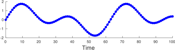
Figure 5. Discrete-time sine wave signal $\mathbf{x}$ defined by (30).

We first analyze a simple sine wave signal similar to (Fainekos and Pappas, 2009a) to illustrate our theoretical findings. Assume we are given the following discrete-time signal:

(30) $$x(t):=\sin(at)+\sin(2at),\quad t=0,\ldots,100$$

where we set $a:=0.1$, see Fig. 5 for an illustration. In the remainder, we consider four different STL specifications $\varphi_{1}$–$\varphi_{4}$.

Specification $\varphi_{1}$. First, we would like to verify that the signal $x(t)$ stays above the threshold $-0.2$ within the first $15$ time units. This can be stated as the STL formula

$$\varphi_{1}:=\square_{[0,\,15]}\,p_{1}$$

where $p_{1}:=x\geq-0.2$. Note that $x$ satisfies $\varphi_{1}$, i.e., $\chi_{\varphi_{1}}(\mathbf{x},0)=1$.

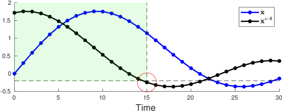
Figure 6. Zoomed in discrete-time sine wave signal $\mathbf{x}$ (blue). The STL formula $\varphi_{1}$ is satisfied with asynchronous temporal robustness $\theta^{+}_{\varphi_{1}}(\mathbf{x},0)=7$. For the signal $\mathbf{x}$ that is shifted by $8$ time units to the left (black), the STL formula $\varphi_{1}$ is violated. Violation is depicted in red where $\mathbf{x}^{\leftarrow 8}(15)<-0.2$ so that $\chi_{p_{1}}(\mathbf{x}^{\leftarrow 8},15)=-1$ and consequently $\chi_{\varphi_{1}}(\mathbf{x}^{\leftarrow 8},0)=-1$.

The left asynchronous temporal robustness is $\theta^{+}_{\varphi_{1}}(\mathbf{x},0)=7$ where the calculation of $\theta^{+}_{\varphi_{1}}(\mathbf{x},0)$ took $0.002$ seconds. We remark that low computation times are obtained throughout this section. Note that since $\varphi_{1}\in\text{STL}^{\!+}(\wedge,\square_{I})$ and $\chi_{\varphi_{1}}(\mathbf{x},0)=1$, it holds that $\eta^{+}_{\varphi_{1}}(\mathbf{x},0)=\theta^{+}_{\varphi_{1}}(\mathbf{x},0)=7$ due to Lemma 4.11. Consequently, we have that $\chi_{\varphi_{1}}(\mathbf{x}^{\leftarrow\tau},0)=1$ for each $\tau\in\{0,\ldots,7\}$ due to (15) and (18). In other words, we can shift the signal $x(t)$ by up to $7$ time units without violating the specification $\varphi_{1}$. Due to (15) it also holds that $\chi_{\varphi_{1}}(\mathbf{x}^{\leftarrow 8},0)=-1$ as illustrated in Fig. 6 for $\mathbf{x}^{\leftarrow 8}$ being depicted in black. This means that once we shift by $8$ time units, we violate the specification $\varphi_{1}$.

Specification $\varphi_{2}$. Let us now increase the timing constraint in $\varphi_{1}$ from 15 to 30 time units, i.e., consider instead the STL formula $\varphi_{2}:=\square_{[0,\,30]}\,p_{1}$. Then it follows that the specification $\varphi_{2}$ is violated by $\mathbf{x}$, i.e., $\chi_{\varphi_{2}}(\mathbf{x},0)=-1$. In fact, the left asynchronous temporal robustness is $\theta^{+}_{\varphi_{2}}(\mathbf{x},0)=-6$. Unlike in the previous case, note that we now can not apply Lemma 4.11 anymore since $\chi_{\varphi_{2}}(\mathbf{x},0)=-1$ and it holds that $\theta^{+}_{\varphi_{2}}(\mathbf{x},0)\neq\eta^{+}_{\varphi_{2}}(\mathbf{x},0)$. Particularly, note that the synchronous left temporal robustness is now $\eta^{+}_{\varphi_{2}}(\mathbf{x},0)=-70$.

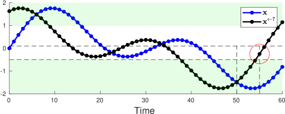
Figure 7. Zoomed in discrete-time sine wave signal $\mathbf{x}$ (blue). The STL formula $\varphi_{3}$ is satisfied with asynchronous temporal robustness $\theta^{+}_{\varphi_{3}}(\mathbf{x},0)=6$. For the signal $\mathbf{x}$ that is shifted by $7$ time units to the left (black), the STL formula $\varphi_{3}$ is violated. Violation is depicted in red, $\mathbf{x}^{\leftarrow 7}(55)>-0.5$.

Specification $\varphi_{3}$. Now, we would like to verify the following property: if in the first 5 time units the value of the signal raises above $0.1$, then it should drop and stay below $-0.5$ from $45$ to $50$ time units. This is expressed by the STL formula

$$\varphi_{3}:=\square_{[0,\,5]}\left(p_{2}\Longrightarrow\square_{[45,\,50]}\;p_{3}\right),$$

where $p_{2}:=x\geq 0.1$ and $p_{3}:=x\leq-0.5$. The left asynchronous temporal robustness for this case is $\theta^{+}_{\varphi_{3}}(\mathbf{x},0)=6$ with a calculation time of $0.005$ seconds. Note that the left synchronous temporal robustness for this case is also $\eta^{+}_{\varphi_{3}}(\mathbf{x},0)=6$ with a computation time of $0.003$ seconds. Consequently, if we shift the signal $\mathbf{x}$ by $7$ time units to the left, i.e. more than the calculated temporal robustness, then the specification $\varphi_{3}$ is not satisfied anymore, see Fig. 7. In fact, one can see that $\mathbf{x}^{\leftarrow 7}(55)>-0.5$. This means that $\chi_{p_{3}}(\mathbf{x}^{\leftarrow 7},55)=-1$ so that $\chi_{\square_{[45,50]}p_{3}}(\mathbf{x}^{\leftarrow 7},5)=-1$ and consequently $\chi_{\varphi_{3}}(\mathbf{x}^{\leftarrow 7},0)=-1$.

Specification $\varphi_{4}$. Consider now a specification $\varphi_{4}$ that depends on a two-dimensional signal. The first component $x_{(1)}(t)$ is equivalent to $x(t)$ in (30), recall Fig. 5, while the second component $x_{(2)}(t)$ is defined as

(31) $$x_{(2)}(t):=\cos(at)-\cos(2at),\quad t=0,\ldots,100$$

where we set $a:=0.1$, see Fig. 8 for an illustration. We also redefine $\mathbf{x}:=(\mathbf{x}_{(1)},\ \mathbf{x}_{(2)})$. We want to verify that during the first ten time units either $x_{(1)}$ is non-positive or $x_{(2)}$ is non-negative which is expressed as

$$\varphi_{4}:=\square_{[0,\,10]}(p_{4}\vee p_{5})$$

where $p_{4}:=x_{(1)}\leq 0$ and $p_{5}:=x_{(2)}\geq 0$.

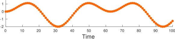
Figure 8. Discrete-time cosine wave signal $\mathbf{x}_{(2)}$ defined by (31).

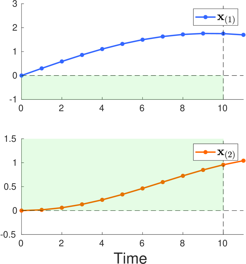
(a) Default signal $\mathbf{x}$. Specification $\varphi_{4}$ is satisfied.

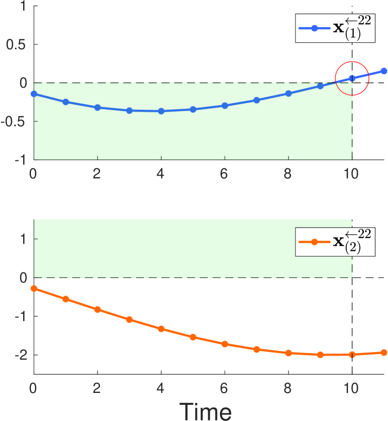
(b) Synchronous early signal $\mathbf{x}^{\leftarrow\tau}$, where $\tau=22$. Specification $\varphi_{4}$ is violated.

Figure 9. Zoomed in analysis of specification $\varphi_{4}$ satisfaction and violation.

The left synchronous temporal robustness for this case is $\eta^{+}_{\varphi_{4}}(\mathbf{x},0)=21$, while the left asynchronous temporal robustness is $\theta^{+}_{\varphi_{4}}(\mathbf{x},0)=10$. Since both values are positive, we can conclude that $\varphi_{4}$ is satisfied due to Theorems 4.1 and 4.5, see Fig. 9(a). Due to (15) for any synchronous early signal $\mathbf{x}^{\leftarrow\tau}$ where $\tau\leq|\eta^{+}_{\varphi_{4}}(\mathbf{x},0)|=21$ it holds that the formula $\varphi_{4}$ will still be satisfied. However, the formula $\varphi_{4}$ will not be satisfied anymore for $\mathbf{x}^{\leftarrow 22}$ which is highlighted in Fig. 9(b). One can indeed see that the specification $\varphi_{4}$ is violated by $\mathbf{x}^{\leftarrow 22}$ since $\mathbf{x}_{(1)}^{\leftarrow 22}(10)>0$ and $\mathbf{x}_{(2)}^{\leftarrow 22}(0),\ldots,\mathbf{x}_{(2)}^{\leftarrow 22}(10)<0$ so that $\chi_{\varphi_{4}}(\mathbf{x}^{\leftarrow 22},0)=-1$. Analogously, we can reason about asynchronous temporal robustness. Since $\theta^{+}_{\varphi_{4}}(\mathbf{x},0)=10$, then for any asynchronous early signal $\mathbf{x}^{\leftarrow\bar{\tau}}$ where $\max(\tau_{p_{4}},\tau_{p_{5}})\leq|\theta^{+}_{\varphi_{4}}(\mathbf{x},0)|=10$ it holds that the formula $\varphi_{4}$ will still be satisfied due to (18).

7.2. Multi-Agent Coordination

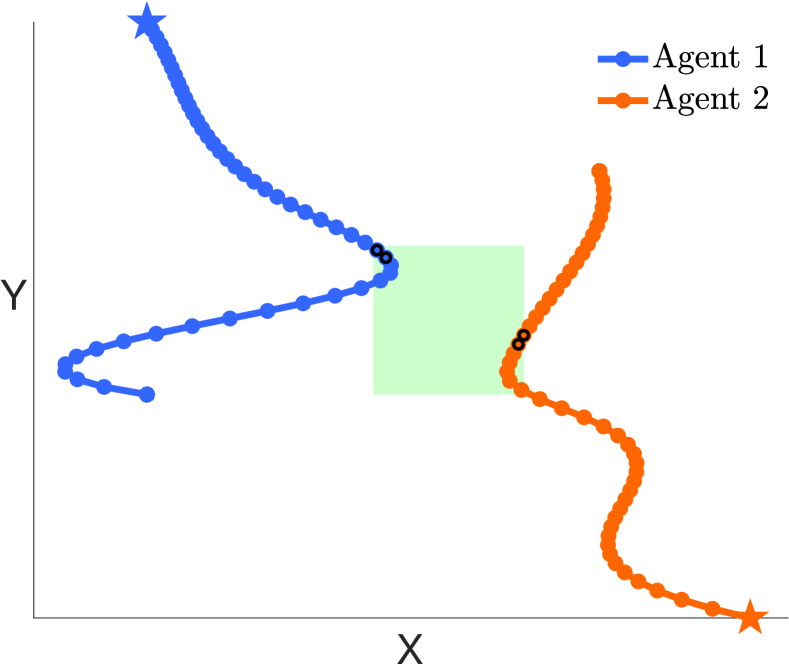
(a) Map and nominal signals.

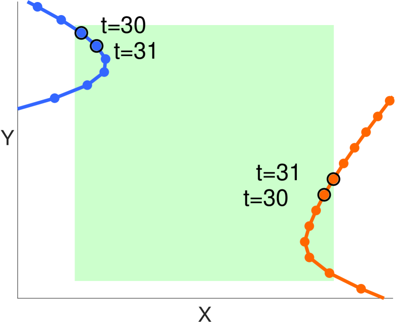
(b) Zoomed in map.

Figure 10. Mission workspace for the multi-agent coordination scenario $\varphi_{\text{coord}}$. Initial positions of the agents marked by $\star$, goal set is given as a green rectangle. Specification $\varphi_{\text{coord}}$ is satisfied by the given nominal signals since there are two time instances when both of the agents are within the goal set (black circles).

In this example, we consider a multi-agent scenario where two agents are supposed to coordinate and exchange goods within a designated goal set and within 50 time units. This scenario is captured in the following specification:

$$\varphi_{\text{coord}}:=\Diamond_{[0,50]}\left(x^{(1)}\in\textit{Goal}\ \wedge\ x^{(2)}\in\textit{Goal}\right)$$

where $x^{(d)}\in\mathbb{R}^{2}$, $d\in\{1,2\}$ denotes the position of the agent $d$ in a two-dimensional space. Fig. 10 depicts the goal set Goal and the given discrete-time signal $\mathbf{x}:=(\mathbf{x}^{(1)},\mathbf{x}^{(2)})$ which has $100$ sampling points. Each $\mathbf{x}^{(d)}$ denotes the position signal of the agent $d$. One can notice that the specification $\varphi_{\text{coord}}$ is satisfied by the nominal signal because there are two time instances ($t=30$ and $t=31$) when both of the agents are within the goal set within the first 50 time units, see Fig. 10(b).

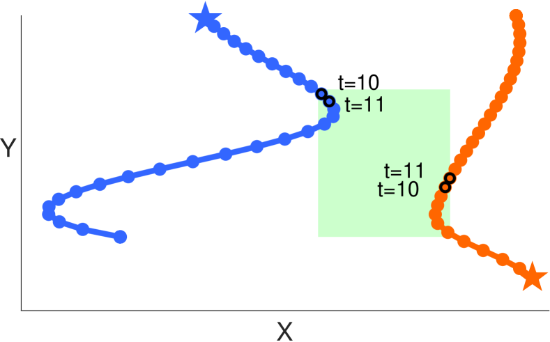
(a) $\mathbf{x}^{\leftarrow\tau},\ \ \tau=20$. Specification $\varphi_{\text{coord}}$ is satisfied by $\mathbf{x}^{\leftarrow 20}$ since there are two time instances when both of the agents are within the goal set.

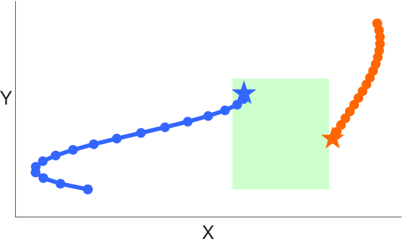
(b) $\mathbf{x}^{\leftarrow\tau},\ \ \tau=32$. Specification $\varphi_{\text{coord}}$ is violated by $\mathbf{x}^{\leftarrow 32}$ since agents are never together in the goal set.

Figure 11. Synchronous early signals.

The calculated left synchronous temporal robustness for this case is $\eta^{+}_{\varphi_{\text{coord}}}(\mathbf{x},0)=31$ time units. Due to Theorem 4.1 the specification $\varphi_{\text{coord}}$ is indeed satisfied, i.e., $\chi_{\varphi_{\text{coord}}}(\mathbf{x},0)=1$. Then due to (15), for any synchronous $\tau$-early signal with $\tau\leq 31$ time units the specification $\varphi_{\text{coord}}$ will still be satisfied. For the signal $\mathbf{x}^{\leftarrow 32}$, however, the specification $\varphi_{\text{coord}}$ will change its satisfaction to violation, i.e.

$$\forall\tau\in[0,31],\ \chi_{\varphi_{\text{coord}}}(\mathbf{x}^{\leftarrow\tau},0)=1\quad\text{and}\quad\chi_{\varphi_{\text{coord}}}(\mathbf{x}^{\leftarrow 32},0)=-1.$$

Fig. 11 depicts two examples of synchronous early signals. Fig. 11(a) shows the signal $\mathbf{x}^{\leftarrow 20}$ for which the specification $\varphi_{\text{coord}}$ is satisfied, and Fig. 11(b) shows $\mathbf{x}^{\leftarrow 32}$ for which $\varphi_{\text{coord}}$ is violated.

(a) $\mathbf{x}^{\leftarrow\bar{\tau}},\ \ \bar{\tau}=(2,0)$. Specification $\varphi_{\text{coord}}$ is satisfied by $\mathbf{x}^{\leftarrow(2,0)}$ since there are four time instances when both of the agents are within the goal set.

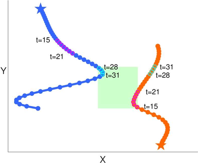
(b) $\mathbf{x}^{\leftarrow\bar{\tau}},\ \ \bar{\tau}=(2,10)$. Specification $\varphi_{\text{coord}}$ is violated by $\mathbf{x}^{\leftarrow(2,10)}$ since agents are never together in the goal set.

Figure 12. Asynchronous early signals.

Due to Theorem 4.10, one can immediately see that $\theta^{+}_{\varphi_{\text{coord}}}(\mathbf{x},0)\leq 31$. Now, since $\varphi\not\in\text{STL}^{\!+}(\wedge,\square_{I})$ it does not necessarily hold that $\theta^{+}_{\varphi_{\text{coord}}}(\mathbf{x},0)=31$. In fact, we find that $\theta^{+}_{\varphi_{\text{coord}}}(\mathbf{x},0)=1$ so that only asynchronous time shifts by up to $1$ time unit to the left will not violate the specification, i.e. $\forall\bar{\tau}\in\{(0,0),(0,1),(1,0),(1,1)\}$ it holds that $\chi_{\varphi_{\text{coord}}}(\mathbf{x}^{\leftarrow\bar{\tau}},0)=1$. As discussed before, (18) only provides a sufficient condition so that asynchronous time shifts larger than $\theta^{+}_{\varphi_{\text{coord}}}(\mathbf{x},0)$ do not necessarily result in a violation of $\varphi_{\text{coord}}$. Indeed, Fig. 12(a) depicts $\mathbf{x}^{\leftarrow(2,0)}$ for which the specification $\varphi_{\text{coord}}$ is satisfied since there are four time instances (black circles) for which both agents are inside the goal set. On the other hand, a simple search over the whole space of possible asynchronous time shifts let us find a signal when the specification $\varphi_{\text{coord}}$ becomes violated, see Fig. 12(b). For $\mathbf{x}^{\leftarrow(2,10)}$, the agents are never together in the goal set: when agent $2$ is inside the goal set (magenta circles), agent $1$ is still on the way to the goal set and the moment agent $1$ reaches the goal (cyan circles), agent $2$ already leaves it.

7.3. Multi-Agent Surveillance

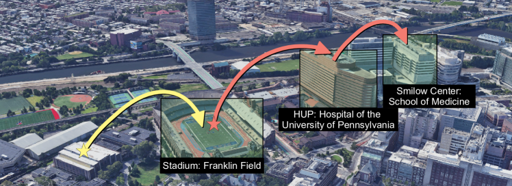
Figure 13. Multi-Agent Surveillance case study map. Initial positions for the two UAVs marked by $\star$.

In this case study we illustrate the control design tools proposed in Section 6. We consider two identical unmanned aerial vehicles (UAVs) and three places of interest on the campus of the University of Pennsylvania, see Fig. 13 for an overview. In particular, these places of interest are the Franklin Field (Stadium), the Hospital of the University of Pennsylvania (HUP), and the School of Medicine Smilow Center (Smilow). The UAVs are tasked with a mission where they collaboratively surveil the Stadium while one of the UAVs is required to pick-up specific items in the HUP and then drop them off at the Smilow.

We assume that the UAVs operate in a two dimensional workspace. For each UAV $d\in\{1,2\}$, let the state be $x^{(d)}:=(pos^{(d)},vel^{(d)})\in\mathbb{R}^{4}$ where $pos^{(d)}$ and $vel^{(d)}$ are the two-dimensional position and velocity, respectively, and let the control input be $u^{(d)}\in\mathbb{R}^{2}$. We denote the full state of the system as $x:=(x^{(1)},x^{(2)})$ and the stacked control input as $u:=(u^{(1)},u^{(2)})$. The linear state-space representation of the system is driven by discrete-time double integrator dynamics and is written as follows:

$$x_{t+1}:=Ax_{t}+Bu_{t},\quad||u_{t}||_{\infty}\leq 20,$$

where $A:=I_{4}\otimes\begin{bmatrix}1&0.1\\ 0&1\end{bmatrix}$ and $B:=I_{4}\otimes\begin{bmatrix}0.005\\ 0.1\end{bmatrix}$ with $I_{n}$ being the identity matrix of dimension $n\times n$ and with $\otimes$ denoting the Kronecker product. We set the time horizon to $H:=50$. The initial positions of the agents are set to $pos_{0}^{(1)}:=(1,3)$ and $pos_{0}^{(2)}:=(8,3)$ (this UAV starts from within the Stadium), while the initial velocities are set to zero.

The overall multi-agent surveillance mission is defined as:

(32) $$\varphi_{\text{MAS}}:=\varphi_{\text{surveil}}\wedge\varphi_{\text{pick-up}}\wedge\varphi_{\text{drop-off}}$$

where we explain $\varphi_{\text{surveil}}$, $\varphi_{\text{pick-up}}$, and $\varphi_{\text{drop-off}}$ in the remainder. The surveillance sub-mission $\varphi_{\text{surveil}}$ requires the Stadium region to be surveilled by at least one UAV for the first 35 time steps. Formally, it is defined as:

$$\varphi_{\text{surveil}}:=\square_{[0,\,35]}(pos^{(1)}\in\textit{Stadium}\ \vee\ pos^{(2)}\in\textit{Stadium}).$$

where Stadium is a rectangle, i.e., $pos^{(d)}\in\textit{Stadium}$ is a conjunction of four linear predicates $x^{(d)}\leq 10$, $x^{(d)}\geq 6$, $y^{(d)}\leq 5$, $y^{(d)}\geq 1$, see Fig. 14.

The second submissions $\varphi_{\text{pick-up}}$ and $\varphi_{\text{drop-off}}$ specify that the second UAV must reach HUP for a pick-up between 10 to 20 time steps. It is required to stay there for 5 time steps which are needed for the loading before departing to Smilow where it suppose to spend all the time between $30$ to $35$ time steps needed for a drop-off. These two sub-missions are formally defined as follows:

$$\varphi_{\text{pick-up}}:=\Diamond_{[10,20]}\square_{[0,\,5]}(pos^{(2)}\in\textit{HUP})$$

$$\varphi_{\text{drop-off}}:=\square_{[30,\,35]}(pos^{(2)}\in\textit{Smilow})$$

Now, in order to generate optimal control inputs, we solve Problem 1 for two different objectives: the left synchronous temporal robustness according to Section 6.2 and the left asynchronous temporal robustness according to Section 6.3.

Figure 14. The nominal UAV trajectories under the optimal control inputs generated by solving Problem 1 with the left synchronous temporal robustness as an objective. The achieved robustness is $\eta^{+}_{\varphi_{\text{MAS}}}(\mathbf{x}_{\text{sync}},0)=10$ time steps. The initial positions are marked by $\star$.

First, we solved Problem 1 with the left synchronous temporal robustness objective, $\vartheta:=\eta^{+}_{\varphi_{\text{MAS}}}$, horizon $H:=50$ and the desired temporal robustness lower bound $\vartheta^{*}:=1$. It led to the optimal trajectory $\mathbf{x}_{\text{sync}}$ and the left temporal robustness value of $\eta^{+}_{\varphi_{\text{MAS}}}(\mathbf{x}_{\text{sync}},0)=10$ time units. The visualization of $\mathbf{x}_{\text{sync}}$ is presented in Fig. 14 and simulation is available at https://tinyurl.com/syncrobust. In Table 3, we show that the solver takes only $0.7$ seconds on average to solve Problem 1 after the problem has been defined using YALMIP, which takes additional $0.65$ seconds. The implementation results in 1165 Boolean and 226 integer variables. Since $\eta^{+}_{\varphi_{\text{MAS}}}(\mathbf{x}_{\text{sync}},0)>0$ the produced optimal signal $\mathbf{x}_{\text{sync}}$ leads to a satisfaction of the mission $\varphi_{\text{MAS}}$. Furthermore, any time disturbances that could lead to $\tau$-early signals by up to $\tau=10$ time steps would still be tolerated by the system and lead to a satisfaction of $\varphi_{\text{MAS}}$, as analyzed in the two previous case studies.

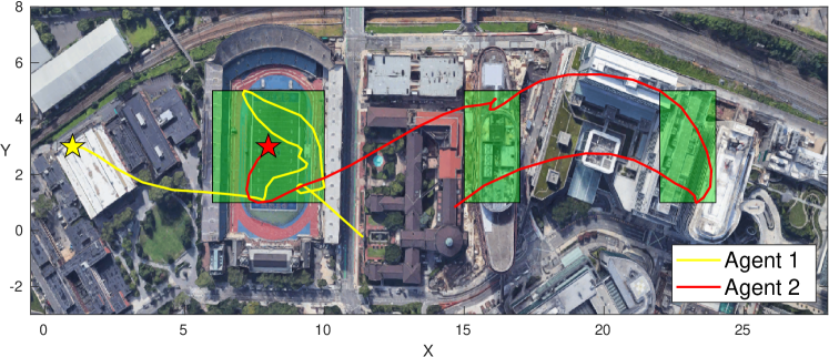
Figure 15. Nominal UAV trajectories under the control policies generated by solving Problem 1 with the left asynchronous temporal robustness. The found robustness value is $\theta^{+}_{\varphi_{\text{MAS}}}(\mathbf{x}_{\text{asyn}},0)=4$ time steps. Initial positions marked by $\star$.

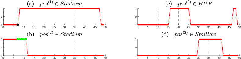
Figure 16. Characteristic function evolution of four predicates consisting in $\varphi_{\text{MAS}}$ over the signal $\mathbf{x}_{\text{asyn}}$. Found maximum left asynchronous temporal robustness is $\theta^{+}_{\varphi_{\text{MAS}}}(\mathbf{x}_{\text{asyn}},0)=4$. For a predicate $p_{2}:=pos^{(2)}\in Stadium$, the five points depicted in green show that only four time steps into the future can be done from time $t=7$ before $p_{2}$ satisfaction changes, therefore, $\theta^{+}_{\varphi_{\text{MAS}}}(\mathbf{x}_{\text{asyn}},0)=\theta^{+}_{p_{2}}(\mathbf{x}_{\text{asyn}},7)=4$.

Next, we solved Problem 1 with the left asynchronous temporal robustness objective, $\vartheta:=\theta^{+}_{\varphi_{\text{MAS}}}$, same horizon $H:=50$ and the same desired temporal robustness lower bound $\vartheta^{*}:=1$. It led to the optimal signal $\mathbf{x}_{\text{asyn}}$ presented in Fig. 15 and the left temporal robustness value of $\theta^{+}_{\varphi_{\text{MAS}}}(\mathbf{x}_{\text{asyn}},0)=4$ time steps, see Fig. 16 for the evaluation of the predicate signals. Simulation is available at https://tinyurl.com/asynrob. In Table 3, we show that the maximization of $\theta^{+}_{\varphi_{\text{MAS}}}(\mathbf{x},0)$ is more computationally challenging than the previous maximization of $\eta^{+}_{\varphi_{\text{MAS}}}(\mathbf{x},0)$. It results in 2026 Boolean and 2095 integer variables and the solver needs $69.6$ seconds on average to solve Problem 1. This result is expected as previously analyzed in Propositions 6.1 and 6.3 where the number of binary and integer variables required for the MILP encoding of $\theta^{+}_{\varphi_{\text{MAS}}}(\mathbf{x})$ is a function of $O(H\cdot(|AP|+|\varphi_{\text{MAS}}|))$, while the MILP encoding of $\eta^{+}_{\varphi_{\text{MAS}}}(\mathbf{x})$ is computationally more tractable and requires only $O(H\cdot|AP|)$ binary and $O(H\cdot|\varphi_{\text{MAS}}|)$ integer variables.

Let us now look at Fig. 15 and denote the predicates $p_{1}:=pos^{(1)}\in Stadium$ and $p_{2}:=pos^{(2)}\in Stadium$. Then from Fig.15 (a) one can see that $\chi_{p_{1}}(\mathbf{x}_{\text{asyn}},t)=-1$ for all time points $t=0,\ldots,7$ but $\chi_{p_{2}}(\mathbf{x}_{\text{asyn}},t)=1$ for $t=0,\ldots,11$. Therefore, $\theta^{+}_{p_{1}\vee p_{2}}(\mathbf{x}_{\text{asyn}},7)=\max(\theta^{+}_{p_{1}}(\mathbf{x}_{\text{asyn}},7),\theta^{+}_{p_{2}}(\mathbf{x}_{\text{asyn}},7))=\max(0,4)=4$, and thus, $\theta^{+}_{\varphi_{\text{MAS}}}(\mathbf{x}_{\text{asyn}},0)=\theta^{+}_{\varphi_{\text{surveil}}}(\mathbf{x}_{\text{asyn}},0)=4$.

The fact, that $\theta^{+}_{\varphi_{\text{MAS}}}(\mathbf{x},0)<10$ is expected due to Theorem 4.10. Adding the constraint $\theta^{+}_{\varphi_{\text{MAS}}}(\mathbf{x},0)<10$ to the overall MILP implementation of Problem 1 with the left asynchronous temporal robustness objective leads to a problem with $11144$ constraints but faster solver computation time, $61.6$ seconds on average, see Table 3.

Mission	Temp. Robustness (time units)	# Constraints	# Variables		Computation time (s)
			Boolean	Integer	YALMIP	Solver
$\varphi_{\text{MAS}}$	$\eta^{+}_{\varphi_{\text{MAS}}}(\mathbf{x}_{\text{sync}},0)=10$	4,597	1165	226	0.65$\pm$0.1	0.7$\pm$0.15
	$\theta^{+}_{\varphi_{\text{MAS}}}(\mathbf{x}_{\text{asyn}},0)=4$	11,143	2026	2095	1$\pm$0.14	69.6$\pm$37.2
$\varphi_{\text{MAS}}$ $\theta^{+}_{\varphi_{\text{MAS}}}(\mathbf{x},0)<10$	$\theta^{+}_{\varphi_{\text{MAS}}}(\mathbf{x}_{\text{asyn}},0)=4$	11,144	2026	2095	1$\pm$0.16	61.6$\pm$31.9

Table 3. Computational complexity report. Computation time includes mean $\pm$ standard deviation of YALMIP time (the time used to build the MILP and convert it into appropriate format for the solver) and Solver time (the time taken by Gurobi to solve the problem). Results obtained from 100 runs of Problem 1 with initial positions chosen at random in small proximity of $pos_{0}^{(1)}$ and $pos_{0}^{(2)}$.

8. Conclusions and future work

This work presents a theoretical framework for temporal robustness of Signal Temporal Logic (STL) specifications which are interpreted over continuous and discrete time signals. In particular we defined synchronous and asynchronous temporal robustness and showed that these notions quantify the robustness with respect to synchronous and asynchronous time shifts in the predicates of signal temporal logic specifications.

For both notions of temporal robustness, we analyzed their desirable properties and showed that the asynchronous temporal robustness is upper bounded by the synchronous temporal robustness in its absolute value. We further showed two particular STL fragments for which the two robustness notions are equivalent.

We further addressed the control synthesis problem in which we aim to design a control law that maximizes the temporal robustness of a dynamical system. We presented Mixed-Integer Linear Programming (MILP) encodings for the synchronous and asynchronous temporal robustness that solve the control synthesis problem.

We are currently exploring several future research directions. First, we are interested in the control synthesis problem when considering temporal robustness of stochastic dynamical systems. We also explore STL robustness notions that combine spatial and temporal robustness. Third, we are interested in computationally more tractable solutions to the control synthesis problem with temporal robustness objectives.

Appendix A Proofs of Section 4

A.1. Proof of Theorem 4.1

Follows directly from Def. 3.1. We are going to prove items 1) and 3). Items 2) and 4) can be proven analogously.

Item 1) states that $\eta^{\pm}_{\varphi}(\mathbf{x},t)>0\ \Longrightarrow\ \chi_{\varphi}(\mathbf{x},t)=1$. By Def. 3.1, $\eta^{\pm}_{\varphi}(\mathbf{x},t)=\chi_{\varphi}(\mathbf{x},t)\cdot\sup\{\tau\geq 0\ :\ \forall t^{\prime}\in t\pm[0,\tau],\ \chi_{\varphi}(\mathbf{x},t^{\prime})=\chi_{\varphi}(\mathbf{x},t)\}$. Since $\eta^{\pm}_{\varphi}(\mathbf{x},t)>0$, $\tau\geq 0$ and $\chi\in\{\pm 1\}$, then $\chi_{\varphi}(\mathbf{x},t)=1$.

Item 3) states that $\chi_{\varphi}(\mathbf{x},t)=1\ \Longrightarrow\ \eta^{\pm}_{\varphi}(\mathbf{x},t)\geq 0$. Since $\chi_{\varphi}(\mathbf{x},t)=1$ then by Def. 3.1, $\eta^{\pm}_{\varphi}(\mathbf{x},t)=\sup\{\tau\geq 0\ :\ \forall t^{\prime}\in t\pm[0,\tau],\ \chi_{\varphi}(\mathbf{x},t^{\prime})=1\}\geq 0$.

A.2. Proof of Corollary 4.2

Corollary 4.2 is a direct consequence of Theorem 4.1. Let $\varphi$ be an STL formula, $\mathbf{x}:\mathbb{T}\rightarrow X$ be a signal and $t\in\mathbb{T}$ be a time point.

1. First, we are going to prove $\eta^{\pm}_{\varphi}(\mathbf{x},t)>0\ \Longrightarrow\ \eta^{\mp}_{\varphi}(\mathbf{x},t)\geq 0$. The following sequence holds:

   $\eta^{\pm}_{\varphi}(\mathbf{x},t)>0\quad\overset{\text{Thm.}\ref{thm:sat_eta}(\ref{ti1})}{\Longrightarrow}\chi_{\varphi}(\mathbf{x},t)=+1\overset{\text{Thm.}\ref{thm:sat_eta}(\ref{ti3})}{\Longrightarrow}\quad\eta^{\mp}_{\varphi}(\mathbf{x},t)\geq 0$.

2. Second, we are going to prove $\eta^{\pm}_{\varphi}(\mathbf{x},t)<0\ \Longrightarrow\ \eta^{\mp}_{\varphi}(\mathbf{x},t)\leq 0$. The following sequence holds:

   $\eta^{\pm}_{\varphi}(\mathbf{x},t)<0\quad\overset{\text{Thm.}\ref{thm:sat_eta}(\ref{ti2})}{\Longrightarrow}\chi_{\varphi}(\mathbf{x},t)=-1\overset{\text{Thm.}\ref{thm:sat_eta}(\ref{ti4})}{\Longrightarrow}\quad\eta^{\mp}_{\varphi}(\mathbf{x},t)\leq 0$.

A.3. Proof of Theorem 4.3

Let $\varphi$ be an STL formula, $\mathbf{x}:\mathbb{R}\rightarrow X$ be a continuous-time signal and $t\in\mathbb{R}$ be a time point. For any value $r\in\overline{\mathbb{R}}_{\geq 0}$, we want to prove that the synchronous temporal robustness $|\eta^{\pm}_{\varphi}(\mathbf{x},t)|=r$ if and only if $\forall t^{\prime}\in t\pm[0,r)$, $\chi_{\varphi}(\mathbf{x},t^{\prime})=\chi_{\varphi}(\mathbf{x},t)$ and if $r<\infty$ then $\forall\epsilon>0$, $\exists\tau\in[r,r+\epsilon)$, $\chi_{\varphi}(\mathbf{x},t\pm\tau)\not=\chi_{\varphi}(\mathbf{x},t)$.

Let $|\eta^{\pm}_{\varphi}(\mathbf{x},t)|=r$. Denote the set $\varUpsilon=\{\tau\geq 0\ :\ \forall t^{\prime}\in t\pm[0,\tau],\ \chi_{\varphi}(\mathbf{x},t^{\prime})=\chi_{\varphi}(\mathbf{x},t)\}$. To prove the result we distinguish between the cases of $r=\infty$ and $r<\infty$ as following:

$(1)$ Let $r=\infty$. Then by Def. 3.1, $\sup\varUpsilon=|\eta^{\pm}_{\varphi}(\mathbf{x},t)|=\infty$. Therefore, we have to show that

$$\sup\varUpsilon=\infty\ \Longleftrightarrow\ \forall t^{\prime}\in t\pm[0,\infty),\ \chi_{\varphi}(\mathbf{x},t^{\prime})=\chi_{\varphi}(\mathbf{x},t)$$

which follows from the definition of the supremum for the unbounded set.

$(2)$ Let $r<\infty$. Then we must show that

(33) $$\sup\varUpsilon=r\quad\Longleftrightarrow \forall t^{\prime}\in t\pm[0,r),\ \chi_{\varphi}(\mathbf{x},t^{\prime})=\chi_{\varphi}(\mathbf{x},t)\qquad\text{and}$$

$$\forall\epsilon>0,\ \exists\tau\in[r,r+\epsilon),\ \chi_{\varphi}(\mathbf{x},t\pm\tau)\not=\chi_{\varphi}(\mathbf{x},t).$$

We next prove sufficiency ($\Longrightarrow$) and necessity ($\Longleftarrow$) of (33) as following:

$\Longrightarrow$ Let $\sup\varUpsilon=r$. Since $r<\infty$ we can apply the $\epsilon$ definition of supremum: $\forall\epsilon>0$, $\exists\tau^{*}\in\varUpsilon$ such that $\tau^{*}>r-\epsilon$. i.e. the following holds:

$$\forall\epsilon>0,\ \exists\tau^{*}\geq 0,\ \tau^{*}>r-\epsilon\ \text{such that}\ \forall t^{\prime}\in t\pm[0,\tau^{*}],\ \chi_{\varphi}(\mathbf{x},t^{\prime})=\chi_{\varphi}(\mathbf{x},t).$$

Since $[0,r-\epsilon]\subset[0,\tau^{*}]$ then it holds that

(34) $$\forall\epsilon>0,\ \forall t^{\prime}\in t\pm[0,r-\epsilon],\ \chi_{\varphi}(\mathbf{x},t^{\prime})=\chi_{\varphi}(\mathbf{x},t).$$

• First, we want to prove that the first line of the RHS of (33) holds, i.e., we want to show that $\forall t^{\prime}\in t\pm[0,r),\ \chi_{\varphi}(\mathbf{x},t^{\prime})=\chi_{\varphi}(\mathbf{x},t)$. Assume the opposite, i.e. assume that $\exists\tau^{*}\in[0,r)$ such that $\chi_{\varphi}(\mathbf{x},t\pm\tau^{*})\not=\chi_{\varphi}(\mathbf{x},t)$. We can represent such $\tau^{*}=r-\epsilon^{*}$ for some $\epsilon^{*}$, $0<\epsilon^{*}\leq r$. Then due to (34), $\forall t^{\prime}\in t\pm[0,r-\epsilon^{*}]$, $\chi_{\varphi}(\mathbf{x},t^{\prime})=\chi_{\varphi}(\mathbf{x},t)$, which contradicts with the above $\chi_{\varphi}(\mathbf{x},t\pm\tau^{*})\not=\chi_{\varphi}(\mathbf{x},t)$. Thus, it indeed holds that:

  (35) $$\forall t^{\prime}\in t\pm[0,r),\ \chi_{\varphi}(\mathbf{x},t^{\prime})=\chi_{\varphi}(\mathbf{x},t).$$

• Second, we want to prove that the second line of the RHS of (33) holds, i.e., we want to show that $\forall\epsilon>0,\ \exists\tau\in[r,r+\epsilon),\ \chi_{\varphi}(\mathbf{x},t\pm\tau)\not=\chi_{\varphi}(\mathbf{x},t)$. Assume the opposite, i.e. assume $\exists\epsilon^{*}>0$, $\forall\tau\in[r,r+\epsilon^{*})$, $\chi_{\varphi}(\mathbf{x},t\pm\tau)=\chi_{\varphi}(\mathbf{x},t)$, which can be rewritten as $\exists\epsilon^{*}>0$, $\forall t^{\prime}\in t\pm[r,r+\epsilon^{*})$, $\chi_{\varphi}(\mathbf{x},t^{\prime})=\chi_{\varphi}(\mathbf{x},t)$. In combination with $\eqref{eq:t1}$, we get $\exists\epsilon^{*}>0$, $\forall t^{\prime}\in t\pm[0,r+\epsilon^{*}),\ \chi_{\varphi}(\mathbf{x},t^{\prime})=\chi_{\varphi}(\mathbf{x},t)$. Since $\epsilon^{*}>0$ then $\tau^{*}=r+\frac{\epsilon^{*}}{2}\in[0,r+\epsilon^{*})$ and $\tau^{*}\geq 0$, therefore, $\tau^{*}\in\varUpsilon$ but also, $\tau^{*}>r$ which is a contradiction, since any value $\tau\in\varUpsilon$ should be $\tau\leq r$ (since $\sup\varUpsilon=r$). Thus, it indeed holds that $\forall\epsilon>0$, $\exists\tau\in[r,r+\epsilon)$, $\chi_{\varphi}(\mathbf{x},t\pm\tau)\not=\chi_{\varphi}(\mathbf{x},t)$.

$\Longleftarrow$ Let $\forall t^{\prime}\in t\pm[0,r),\ \chi_{\varphi}(\mathbf{x},t^{\prime})=\chi_{\varphi}(\mathbf{x},t)$ and $\forall\epsilon>0,\ \exists\tau\in[r,r+\epsilon),\ \chi_{\varphi}(\mathbf{x},t\pm\tau)\not=\chi_{\varphi}(\mathbf{x},t)$, where $r<\infty$. Blow we show that $\sup\varUpsilon=r$.

• First, we are going to show that $\forall s\in\varUpsilon$, $s\leq r$. Assume the opposite, assume $\exists s=s^{*}\in\varUpsilon$ such that $s^{*}>r$. From the definition of $\varUpsilon$ this can be rewritten as $\exists s^{*}(s^{*}>r\ \wedge\ \forall t^{\prime}\in t\pm[0,s^{*}],\ \chi_{\varphi}(\mathbf{x},t^{\prime})=\chi_{\varphi}(\mathbf{x},t))$. Take $\epsilon=s^{*}-r$. Since $s^{*}>r$, $\epsilon>0$, therefore, from what is given, $\exists\tau\in[r,r+\epsilon)=[r,s^{*}),\ \chi_{\varphi}(\mathbf{x},t\pm\tau)\not=\chi_{\varphi}(\mathbf{x},t)$. But since $[r,s^{*})\subset[0,s^{*}]$ then $\tau\in[0,s^{*}]$ which is a contradiction with the assumed. Therefore, it indeed holds that $\forall s\in\varUpsilon$, $s\leq r$.

• Second, we are going to show that $\forall\epsilon>0$, $\exists\tau^{*}\in\varUpsilon$ such that $\tau^{*}>r-\epsilon$. Take any $\epsilon>0$.

  • If $r<\frac{\epsilon}{2}$, i.e. $r-\epsilon<r-\frac{\epsilon}{2}<0$ then let $\tau^{*}=0$. In this case, $\tau^{*}\in\varUpsilon$ and $\tau^{*}>r-\epsilon$.

  • If $r\geq\frac{\epsilon}{2}$, then let $\tau^{*}=r-\frac{\epsilon}{2}$. In this case, $\tau^{*}\geq 0$ and $\tau^{*}=r-\frac{\epsilon}{2}>r-\epsilon$. Also, we know that $\forall t^{\prime}\in t\pm[0,r),\ \chi_{\varphi}(\mathbf{x},t^{\prime})=\chi_{\varphi}(\mathbf{x},t)$. Since $[0,r-\frac{\epsilon}{2}]\subset[0,r)$ then $\forall t^{\prime}\in t\pm[0,\tau^{*}]$, $\chi_{\varphi}(\mathbf{x},t^{\prime})=\chi_{\varphi}(\mathbf{x},t)$, i.e. $\tau^{*}\in\varUpsilon$.

Thus, $\sup\varUpsilon=r$ which concludes the proof.

A.4. Proof of Eq.(9) (Theorem 4.3 for discrete-time)

Let $\varphi$ be an STL formula, $\mathbf{x}:\mathbb{Z}\rightarrow X$ be a discrete-time signal and $t\in\mathbb{Z}$ be a time point. For any finite value $r\in\mathbb{Z}_{\geq 0}$, we want to prove that the synchronous temporal robustness $|\eta^{\pm}_{\varphi}(\mathbf{x},t)|=r$ if and only if $\forall t^{\prime}\in t\pm[0,r]$, $\chi_{\varphi}(\mathbf{x},t^{\prime})=\chi_{\varphi}(\mathbf{x},t)$ and $\chi_{\varphi}(\mathbf{x},t\pm(r+1))\not=\chi_{\varphi}(\mathbf{x},t)$.

Let $|\eta^{\pm}_{\varphi}(\mathbf{x},t)|=r$. Denote the set $\varUpsilon=\{\tau\geq 0\ :\ \forall t^{\prime}\in t\pm[0,\tau],\ \chi_{\varphi}(\mathbf{x},t^{\prime})=\chi_{\varphi}(\mathbf{x},t)\}$. Then, by Def. 3.1, $|\eta^{\pm}_{\varphi}(\mathbf{x},t)|=\sup\varUpsilon=r$. Since $r$ is finite and $t\in\mathbb{Z}$ then it holds that $\sup\varUpsilon=\max\varUpsilon=r$, which holds if and only if $\forall t^{\prime}\in t\pm[0,r]$, $\chi_{\varphi}(\mathbf{x},t^{\prime})=\chi_{\varphi}(\mathbf{x},t)$ and $\chi_{\varphi}(\mathbf{x},t\pm(r+1))\not=\chi_{\varphi}(\mathbf{x},t)$.

A.5. Proof of Theorem 4.4

Let $\varphi$ be an STL formula, $\mathbf{x}:\mathbb{R}\rightarrow X$ be a continuous-time signal and $t\in\mathbb{R}$ be a time point. For any value $r\in\overline{\mathbb{R}}_{\geq 0}$, we want to prove that if the synchronous temporal robustness $|\eta^{\pm}_{\varphi}(\mathbf{x},t)|=r$ then $\forall\tau\in[0,r)$, $|\eta^{\pm}_{\varphi}(\mathbf{x},t\pm\tau)|=r-\tau$.

Let $|\eta^{\pm}_{\varphi}(\mathbf{x},t)|=r\geq 0$. To prove the result we distinguish between the cases of $r=\infty$ and $r<\infty$:

1. Let $r=\infty$. Then according to Thm. 4.3, $\forall\tau\in[0,\infty),\ \chi_{\varphi}(\mathbf{x},t\pm\tau)=\chi_{\varphi}(\mathbf{x},t)$. Take any $\tau\in[0,\infty)$, then it holds that $\forall\tau^{\prime}\in[0,\infty)$, $\chi_{\varphi}(\mathbf{x},t\pm\tau\pm\tau^{\prime})=\chi_{\varphi}(\mathbf{x},t\pm\tau)$. Thus, according to Thm. 4.3, $|\eta^{\pm}_{\varphi}(\mathbf{x},t\pm\tau)|=\infty=\infty-\tau$.

2. Let $r<\infty$. Then according to Thm. 4.3, $\forall\tau\in[0,r),\ \chi_{\varphi}(\mathbf{x},t\pm\tau)=\chi_{\varphi}(\mathbf{x},t)$ and $\forall\epsilon>0,\ \exists\tilde{\tau}\in[r,r+\epsilon),\ \chi_{\varphi}(\mathbf{x},t\pm\tilde{\tau})\not=\chi_{\varphi}(\mathbf{x},t)$. Take any $\tau\in[0,r)$. Then the first property leads to $\forall\tau^{\prime}\in[0,r-\tau),\ \chi_{\varphi}(\mathbf{x},t\pm\tau\pm\tau^{\prime})=\chi_{\varphi}(\mathbf{x},t\pm\tau)=\chi_{\varphi}(\mathbf{x},t)$. The second property leads to $\forall\epsilon>0,\ \exists\tilde{\tau}\in[r-\tau,r+\epsilon-\tau),\ \chi_{\varphi}(\mathbf{x},t\pm\tau\pm\tilde{\tau})\not=\chi_{\varphi}(\mathbf{x},t)=\chi_{\varphi}(\mathbf{x},t\pm\tau)$. The combination of these two due to Thm. 4.3 leads to $|\eta^{\pm}_{\varphi}(\mathbf{x},t\pm\tau)|=r-\tau$.

A.6. Proof of Eq.(10) (Theorem 4.4 for discrete-time)

Let $\varphi$ be an STL formula, $\mathbf{x}:\mathbb{Z}\rightarrow X$ be a discrete-time signal and $t\in\mathbb{Z}$ be a time point. For any finite value $r\in\mathbb{Z}_{\geq 0}$, we want to prove that if $|\eta^{\pm}_{\varphi}(\mathbf{x},t)|=r$ then $\forall\tau\in[0,r]$, $|\eta^{\pm}_{\varphi}(\mathbf{x},t\pm\tau)|=r-\tau$.

Let $|\eta^{\pm}_{\varphi}(\mathbf{x},t)|=r$. Then according to (9), it holds that $\forall\tau\in[0,r],\ \chi_{\varphi}(\mathbf{x},t\pm\tau)=\chi_{\varphi}(\mathbf{x},t)$ and $\chi_{\varphi}(\mathbf{x},t\pm(r+1))\not=\chi_{\varphi}(\mathbf{x},t)$. Take any $\tau\in[0,r]$. Then the first property leads to $\forall\tau^{\prime}\in[0,r-\tau],\ \chi_{\varphi}(\mathbf{x},t\pm\tau\pm\tau^{\prime})=\chi_{\varphi}(\mathbf{x},t\pm\tau)=\chi_{\varphi}(\mathbf{x},t)$. The second property leads to $\chi_{\varphi}(\mathbf{x},t\pm\tau\pm(r-\tau+1))\not=\chi_{\varphi}(\mathbf{x},t)=\chi_{\varphi}(\mathbf{x},t\pm\tau)$. The combination of these two due to (10) leads to $|\eta^{\pm}_{\varphi}(\mathbf{x},t\pm\tau)|=r-\tau$.

A.7. Proof of Theorem 4.5

In this proof, we will use the following lemma.

Lemma A.1.

For a set $S\subseteq\overline{\mathbb{R}}$ if $\sup S>0$ then $\exists s\in S$ such that $s>0$.

Proof.

Let a set $S\subseteq\overline{\mathbb{R}}$ be such that $\sup S>0$. Assume the opposite of what we want to prove, i.e. assume that $\forall s\in S$, $s\leq 0$. Then 0 is an upper bound of $S$. So $\sup S\leq 0$ but we are given $\sup S>0$ which is a contradiction. Therefore, $\exists s\in S$ such that $s>0$. ∎

To prove Thm. 4.5, we are going to prove items 1) and 3). Items 2) and 4) can be proven analogously.

1) We want to prove that $\theta^{\pm}_{\varphi}(\mathbf{x},t)>0\Longrightarrow\chi_{\varphi}(\mathbf{x},t)=1$. Thus, let $\theta^{\pm}_{\varphi}(\mathbf{x},t)>0$. The rest of the proof is by induction on the structure of formula $\varphi$.

1. $\varphi=p$. Since we are given that $\theta^{\pm}_{p}(\mathbf{x},t)>0$, then due to Corollary 4.9, $\eta^{\pm}_{p}(\mathbf{x},t)>0$ which due to Thm. 4.1 leads to $\chi_{p}(\mathbf{x},t)=1$.

2. $\varphi=\neg\varphi_{1}$. Since $\theta^{\pm}_{\neg\varphi_{1}}(\mathbf{x},t)>0$ then due to (6) it holds that $\theta^{\pm}_{\varphi_{1}}(\mathbf{x},t)<0$. By the induction hypothesis for $\varphi_{1}$ we get that $\chi_{\varphi_{1}}(\mathbf{x},t)=-1$, and thus by Def. 2.1, $\chi_{\neg\varphi_{1}}(\mathbf{x},t)=-\chi_{\varphi_{1}}(\mathbf{x},t)=1$.

3. $\varphi=\varphi_{1}\wedge\varphi_{2}$. Since $\theta^{\pm}_{\varphi_{1}\wedge\varphi_{2}}(\mathbf{x},t)=\theta^{\pm}_{\varphi_{1}}(\mathbf{x},t)\ \sqcap\ \theta^{\pm}_{\varphi_{2}}(\mathbf{x},t)>0$, both terms are positive: $\theta^{\pm}_{\varphi_{1}}(\mathbf{x},t)>0$ and $\theta^{\pm}_{\varphi_{2}}(\mathbf{x},t)>0$. By the induction hypothesis we get that $\chi_{\varphi_{1}}(\mathbf{x},t)=\chi_{\varphi_{2}}(\mathbf{x},t)=1$, and thus by Def. 2.1, $\chi_{\varphi}(\mathbf{x},t)=\chi_{\varphi_{1}}(\mathbf{x},t)\sqcap\chi_{\varphi_{2}}(\mathbf{x},t)=1$.

4. $\varphi=\varphi_{1}\mathcal{U}_{I}\varphi_{2}$. Since $\theta^{\pm}_{\varphi}(\mathbf{x},t)>0$ then due to Lemma A.1 and Def. 3.2 for Until operator, $\exists t^{\prime}\in t+I$ such that $\theta^{\pm}_{\varphi_{2}}(\mathbf{x},t^{\prime})\ \sqcap\ \bigsqcap_{t^{\prime\prime}\in[t,t^{\prime})}\theta^{\pm}_{\varphi_{1}}(\mathbf{x},t^{\prime\prime})>0$. Now due to the infimum operators, $\theta^{\pm}_{\varphi_{2}}(\mathbf{x},t^{\prime})>0$ and $\forall t^{\prime\prime}\in[t,t^{\prime})$, $\theta^{\pm}_{\varphi_{1}}(\mathbf{x},t^{\prime\prime})>0$. Therefore, from the induction hypothesis, $\exists t^{\prime}\in t+I$, $\chi_{\varphi_{2}}(\mathbf{x},t^{\prime})=1$ and $\forall t^{\prime\prime}\in[t,t^{\prime})$, $\chi_{\varphi_{1}}(\mathbf{x},t^{\prime\prime})=1$. And thus, $\chi_{\varphi}(\mathbf{x},t)=1$.

3) We want to prove that $\chi_{\varphi}(\mathbf{x},t)=1\Longrightarrow\theta^{\pm}_{\varphi}(\mathbf{x},t)\geq 0$. Thus, let $\chi_{\varphi}(\mathbf{x},t)=1$. The rest of the proof is by induction on the structure of formula $\varphi$.

• $\varphi=p$. Since we are given that $\chi_{p}(\mathbf{x},t)=1$ then due to Thm. 4.1(3) it holds that $\eta^{\pm}_{p}(\mathbf{x},t)\geq 0$ and thus, due to Corollary 4.9, $\theta^{\pm}_{p}(\mathbf{x},t)=\eta^{\pm}_{p}(\mathbf{x},t)\geq 0$.

• $\varphi=\neg\varphi_{1}$. Since we are given that $\chi_{\neg\varphi_{1}}(\mathbf{x},t)=1$ then it holds that $\chi_{\varphi_{1}}(\mathbf{x},t)=-1$. By the induction hypothesis for $\varphi_{1}$, $\theta^{\pm}_{\varphi_{1}}(\mathbf{x},t)\leq 0$, and thus due to (6), $\theta^{\pm}_{\neg\varphi_{1}}(\mathbf{x},t)=-\theta^{\pm}_{\varphi_{1}}(\mathbf{x},t)\geq 0$.

• $\varphi=\varphi_{1}\wedge\varphi_{2}$. Since $\chi_{\varphi}(\mathbf{x},t)=\chi_{\varphi_{1}}(\mathbf{x},t)\sqcap\chi_{\varphi_{2}}(\mathbf{x},t)=1$ then both $\chi_{\varphi_{1}}(\mathbf{x},t)=1$ and $\chi_{\varphi_{2}}(\mathbf{x},t)=1$. By the induction hypothesis we get that $\theta^{\pm}_{\varphi_{1}}(\mathbf{x},t)\geq 0$ and $\theta^{\pm}_{\varphi_{2}}(\mathbf{x},t)\geq 0$ and thus, $\theta^{\pm}_{\varphi}(\mathbf{x},t)=\theta^{\pm}_{\varphi_{1}}(\mathbf{x},t)\sqcap\theta^{\pm}_{\varphi_{2}}(\mathbf{x},t)\geq 0$.

• $\varphi=\varphi_{1}\mathcal{U}_{I}\varphi_{2}$. Since $\chi_{\varphi}(\mathbf{x},t)=1$ then from the definition of the characteristic function for Until operator, $\exists t^{\prime}\in t+I$ such that $\chi_{\varphi_{2}}(\mathbf{x},t^{\prime})=1$ and $\forall t^{\prime\prime}\in[t,t^{\prime})$, $\chi_{\varphi_{1}}(\mathbf{x},t^{\prime\prime})=1$. By the induction hypothesis we obtain that $\exists t^{\prime}\in t+I$ such that $\theta^{\pm}_{\varphi_{2}}(\mathbf{x},t^{\prime})\geq 0$ and $\forall t^{\prime\prime}\in[t,t^{\prime})$, $\theta^{\pm}_{\varphi_{1}}(\mathbf{x},t^{\prime\prime})\geq 0$ and thus, by (8) we conclude that $\theta^{\pm}_{\varphi}(\mathbf{x},t)\geq 0.$

A.8. Proof of Corollary 4.6

Corollary 4.6 is a direct consequence of Theorem 4.5. Let $\varphi$ be an STL formula, $\mathbf{x}:\mathbb{T}\rightarrow X$ be a signal and $t\in\mathbb{T}$ be a time point.

1. First, we are going to prove $\theta^{\pm}_{\varphi}(\mathbf{x},t)>0\ \Longrightarrow\ \theta^{\mp}_{\varphi}(\mathbf{x},t)\geq 0$. The following sequence holds:

   $\theta^{\pm}_{\varphi}(\mathbf{x},t)>0\quad\overset{\text{Thm.}\ref{thm:sat_theta}(\ref{i1})}{\Longrightarrow}\chi_{\varphi}(\mathbf{x},t)=+1\overset{\text{Thm.}\ref{thm:sat_theta}(\ref{i3})}{\Longrightarrow}\quad\theta^{\mp}_{\varphi}(\mathbf{x},t)\geq 0$.

2. Second, we are going to prove $\theta^{\pm}_{\varphi}(\mathbf{x},t)<0\ \Longrightarrow\ \theta^{\mp}_{\varphi}(\mathbf{x},t)\leq 0$. The following sequence holds:

   $\theta^{\pm}_{\varphi}(\mathbf{x},t)<0\quad\overset{\text{Thm.}\ref{thm:sat_theta}(\ref{i2})}{\Longrightarrow}\chi_{\varphi}(\mathbf{x},t)=-1\overset{\text{Thm.}\ref{thm:sat_theta}(\ref{i4})}{\Longrightarrow}\quad\theta^{\mp}_{\varphi}(\mathbf{x},t)\leq 0$.

A.9. Proof of Theorem 4.7

Let $\varphi$ be an STL formula, $\mathbf{x}:\mathbb{R}\rightarrow X$ be a continuous-time signal and $t\in\mathbb{R}$ be a time point. For any value $r\in\overline{\mathbb{R}}_{\geq 0}$, we want to prove that if $|\theta^{\pm}_{\varphi}(\mathbf{x},t)|=r$ then $\forall t^{\prime}\in t\pm\,[0,r)$, $\chi_{\varphi}(\mathbf{x},t^{\prime})=\chi_{\varphi}(\mathbf{x},t)$.

Note that the result is trivial for $r=0$. Therefore, let $|\theta^{\pm}_{\varphi}(\mathbf{x},t)|=r>0$. The rest of the proof is by induction on the structure of the formula $\varphi$.

1. $\varphi=p$. Since $|\theta^{\pm}_{p}(\mathbf{x},t)|=r$ then due to Corollary 4.9, $|\eta^{\pm}_{p}(\mathbf{x},t)|=r$. From Theorem 4.3 we get that $\forall t^{\prime}\in t\pm[0,r),\ \chi_{p}(\mathbf{x},t^{\prime})=\chi_{p}(\mathbf{x},t)$.

2. $\varphi=\neg\varphi_{1}$. Since $|\theta^{\pm}_{\neg\varphi_{1}}(\mathbf{x},t)|=r$ then due to (6) it holds that $|\theta^{\pm}_{\varphi_{1}}(\mathbf{x},t)|=r$. By the induction hypothesis for $\varphi_{1}$ we get that $\forall t^{\prime}\in t\pm[0,r),\ \chi_{\varphi_{1}}(\mathbf{x},t^{\prime})=\chi_{\varphi_{1}}(\mathbf{x},t)$. Therefore, due to Def. 2.1, it holds that $\forall t^{\prime}\in t\pm[0,r)\quad\chi_{\neg\varphi_{1}}(\mathbf{x},t^{\prime})=-\chi_{\varphi_{1}}(\mathbf{x},t^{\prime})=-\chi_{\varphi_{1}}(\mathbf{x},t)=\chi_{\neg\varphi_{1}}(\mathbf{x},t)$.

3. $\varphi=\varphi_{1}\wedge\varphi_{2}$. We consider the two separate cases of $\chi_{\varphi}(\mathbf{x},t)=1$ and $\chi_{\varphi}(\mathbf{x},t)=-1$ as follows:

   1. Let $\chi_{\varphi}(\mathbf{x},t)=1$. Since $|\theta^{\pm}_{\varphi}(\mathbf{x},t)|=r>0$ then due to Thm. 4.5(3), $\theta^{\pm}_{\varphi}(\mathbf{x},t)=r>0$. WLOG assume that $\theta^{\pm}_{\varphi_{1}}(\mathbf{x},t)\leq\theta^{\pm}_{\varphi_{2}}(\mathbf{x},t)$. Therefore, $|\theta^{\pm}_{\varphi}(\mathbf{x},t)|=\theta^{\pm}_{\varphi}(\mathbf{x},t)\overset{\eqref{eq:t_and}}{=}\theta^{\pm}_{\varphi_{1}}(\mathbf{x},t)\ \sqcap\ \theta^{\pm}_{\varphi_{2}}(\mathbf{x},t)=\theta^{\pm}_{\varphi_{1}}(\mathbf{x},t)=r$. If we denote $\theta^{\pm}_{\varphi_{2}}(\mathbf{x},t)=j$ then $0<r=\theta^{\pm}_{\varphi_{1}}(\mathbf{x},t)\leq\theta^{\pm}_{\varphi_{2}}(\mathbf{x},t)=j$. From $r\leq j$ and by the induction hypothesis for $\varphi_{k}$ for $k\in\{1,2\}$ it holds that $\forall t^{\prime}\in t\pm[0,r)$, $\chi_{\varphi_{k}}(\mathbf{x},t^{\prime})=\chi_{\varphi_{k}}(\mathbf{x},t)$. Thus, using Def. 2.1, $\forall t^{\prime}\in t\pm[0,r)$ it holds that $\chi_{\varphi}(\mathbf{x},t^{\prime})=\chi_{\varphi_{1}}(\mathbf{x},t^{\prime})\sqcap\chi_{\varphi_{2}}(\mathbf{x},t^{\prime})=\chi_{\varphi_{1}}(\mathbf{x},t)\sqcap\chi_{\varphi_{2}}(\mathbf{x},t)=\chi_{\varphi}(\mathbf{x},t)$.

   2. Let $\chi_{\varphi}(\mathbf{x},t)=-1$. Since $|\theta^{\pm}_{\varphi}(\mathbf{x},t)|=r>0$ then due to Thm. 4.5(4), $\theta^{\pm}_{\varphi}(\mathbf{x},t)=-r<0$. WLOG assume that $\theta^{\pm}_{\varphi_{1}}(\mathbf{x},t)\leq\theta^{\pm}_{\varphi_{2}}(\mathbf{x},t)$. Therefore, $-|\theta^{\pm}_{\varphi}(\mathbf{x},t)|=\theta^{\pm}_{\varphi}(\mathbf{x},t)\overset{\eqref{eq:t_and}}{=}\theta^{\pm}_{\varphi_{1}}(\mathbf{x},t)\ \sqcap\ \theta^{\pm}_{\varphi_{2}}(\mathbf{x},t)=\theta^{\pm}_{\varphi_{1}}(\mathbf{x},t)=-r<0$. Since $\theta^{\pm}_{\varphi_{1}}(\mathbf{x},t)<0$ then $\chi_{\varphi_{1}}(\mathbf{x},t)=-1$. From the induction hypothesis for $\varphi_{1}$ we get that $\forall t^{\prime}\in t\pm[0,r)$, $\chi_{\varphi_{1}}(\mathbf{x},t^{\prime})=\chi_{\varphi_{1}}(\mathbf{x},t)=-1$. Thus, by Def. 2.1, $\forall t^{\prime}\in t\pm[0,r)$ it holds that $\chi_{\varphi}(\mathbf{x},t^{\prime})=\chi_{\varphi_{1}}(\mathbf{x},t^{\prime})\sqcap\chi_{\varphi_{2}}(\mathbf{x},t^{\prime})=-1\sqcap\chi_{\varphi_{2}}(\mathbf{x},t^{\prime})=-1=\chi_{\varphi}(\mathbf{x},t)$.

4. $\varphi=\varphi_{1}\mathcal{U}_{I}\varphi_{2}$. We consider the two separate cases of $\chi_{\varphi}(\mathbf{x},t)=1$ and $\chi_{\varphi}(\mathbf{x},t)=-1$ as follows:

   1. Let $\chi_{\varphi}(\mathbf{x},t)=1$. Since $|\theta^{\pm}_{\varphi}(\mathbf{x},t)|=r>0$ then due to Thm. 4.5(3), $\theta^{\pm}_{\varphi}(\mathbf{x},t)=r>0$, therefore, due to (8), it holds that $\bigsqcup_{t^{\prime}\in t+I}\left(\theta^{\pm}_{\varphi_{2}}(\mathbf{x},t^{\prime})\ \sqcap\ \bigsqcap_{t^{\prime\prime}\in[t,t^{\prime})}\theta^{\pm}_{\varphi_{1}}(\mathbf{x},t^{\prime\prime})\right)=r>0$. To prove the rest we distinguish between the cases of $r<\infty$ and $r=\infty$ as following:

   1.1. Let $r<\infty$. Then due to the $\epsilon$ definition of the supremum the following holds:

   (36) $$\forall\epsilon>0,\ \exists t^{\prime}\in t+I,\quad\theta^{\pm}_{\varphi_{2}}(\mathbf{x},t^{\prime})\ \sqcap\ \bigsqcap_{t^{\prime\prime}\in[t,t^{\prime})}\theta^{\pm}_{\varphi_{1}}(\mathbf{x},t^{\prime\prime})>r-\epsilon$$

   which by the definition of the infimum ($\forall x,\ \inf f(x)\leq f(x)$) further leads to:

   (37) $$\forall\epsilon>0,\ \exists t^{\prime}\in t+I\ \left(\theta^{\pm}_{\varphi_{2}}(\mathbf{x},t^{\prime})>r-\epsilon\quad\wedge\quad\forall t^{\prime\prime}\in[t,t^{\prime}),\ \theta^{\pm}_{\varphi_{1}}(\mathbf{x},t^{\prime\prime})>r-\epsilon\right)$$

   Note that since $r>0$ then using Thm. 4.5, $\chi_{\varphi_{2}}(\mathbf{x},t^{\prime})=\chi_{\varphi_{1}}(\mathbf{x},t^{\prime\prime})=1$. By the induction hypothesis we get that

   $$\forall\epsilon>0, \exists t^{\prime}\in t+I\ (\forall\tau\in[0,\theta^{\pm}_{\varphi_{2}}(\mathbf{x},t^{\prime})),\ \chi_{\varphi_{2}}(\mathbf{x},t^{\prime}\pm\tau)=1\ \wedge$$

   $$\forall t^{\prime\prime}\in[t,t^{\prime}),\forall\tau\in[0,\theta^{\pm}_{\varphi_{1}}(\mathbf{x},t^{\prime\prime})),\ \chi_{\varphi_{1}}(\mathbf{x},t^{\prime\prime}\pm\tau)=1)$$

   where $\theta^{\pm}_{\varphi_{2}}(\mathbf{x},t^{\prime})>r-\epsilon$ and $\theta^{\pm}_{\varphi_{1}}(\mathbf{x},t^{\prime\prime})>r-\epsilon$. Therefore, $[0,\theta^{\pm}_{\varphi_{2}}(\mathbf{x},t^{\prime}))\supset[0,r-\epsilon)$ and $[0,\theta^{\pm}_{\varphi_{1}}(\mathbf{x},t^{\prime\prime}))\supset[0,r-\epsilon)$. Thus,

   $$\forall\epsilon>0, \exists t^{\prime}\in t+I\ (\forall\tau\in[0,r-\epsilon),\ \chi_{\varphi_{2}}(\mathbf{x},t^{\prime}\pm\tau)=1\ \wedge$$

   $$\forall t^{\prime\prime}\in[t,t^{\prime}),\forall\tau\in[0,r-\epsilon),\ \chi_{\varphi_{1}}(\mathbf{x},t^{\prime\prime}\pm\tau)=1)$$

   Therefore, due to Lemma D.1(1), (3) and (2) it holds that $\forall\epsilon>0$, $\forall\tau\in[0,r-\epsilon)$, $\exists t^{\prime}\in t+I$,

   $$\chi_{\varphi_{2}}(\mathbf{x},t^{\prime}\pm\tau)=1\ \wedge\ \forall t^{\prime\prime}\in[t,t^{\prime}),\ \chi_{\varphi_{1}}(\mathbf{x},t^{\prime\prime}\pm\tau)=1$$

   Thus, by Def. 2.1, $\forall\epsilon>0,\ \forall\tau\in[0,r-\epsilon)$, $\chi_{\varphi}(\mathbf{x},t\pm\tau)=1$, thus, $\forall\tau\in[0,r),\chi_{\varphi}(\mathbf{x},t\pm\tau)=1$.

   1.2. Let $r=\infty$. Then the following holds:

   (38) $$\forall M\in\mathbb{R},\ \exists t^{\prime}\in t+I,\quad\theta^{\pm}_{\varphi_{2}}(\mathbf{x},t^{\prime})\ \sqcap\ \bigsqcap_{t^{\prime\prime}\in[t,t^{\prime})}\theta^{\pm}_{\varphi_{1}}(\mathbf{x},t^{\prime\prime})>M$$

   Which is similar to (36) but uses $M$ instead of $r-\epsilon$. Following the above steps, one can obtain that $\forall M\in\mathbb{R}$, $\forall\tau\in[0,M)$, $\chi_{\varphi}(\mathbf{x},t\pm\tau)=1$, i.e. $\forall\tau\in[0,\infty)$, $\chi_{\varphi}(\mathbf{x},t\pm\tau)=1$.

   2. Let $\chi_{\varphi}(\mathbf{x},t)=-1$. Since $|\theta^{\pm}_{\varphi}(\mathbf{x},t)|=r>0$ then due to Thm. 4.5(4), $\theta^{\pm}_{\varphi}(\mathbf{x},t)=-r<0$, therefore, due to (8), it holds that $\bigsqcup_{t^{\prime}\in t+I}\left(\theta^{\pm}_{\varphi_{2}}(\mathbf{x},t^{\prime})\ \sqcap\ \bigsqcap_{t^{\prime\prime}\in[t,t^{\prime})}\theta^{\pm}_{\varphi_{1}}(\mathbf{x},t^{\prime\prime})\right)=-r<0$. To prove the rest we distinguish between the cases of $r=\infty$ and $r<\infty$ as following:

   2.1 Let $r=\infty$. Then we conclude that $\forall t^{\prime}\in t+I$, $\theta^{\pm}_{\varphi_{2}}(\mathbf{x},t^{\prime})=-\infty$ or $\bigsqcap_{t^{\prime\prime}\in[t,t^{\prime})}\theta^{\pm}_{\varphi_{1}}(\mathbf{x},t^{\prime\prime})=-\infty$. Therefore, by the definition of an infimum (unbounded set), the following holds:

   (39) $$\forall t^{\prime}\in t+I\ \left(\theta^{\pm}_{\varphi_{2}}(\mathbf{x},t^{\prime})=-\infty\ \vee\ \forall M\in\mathbb{R}_{+},\ \exists t^{\prime\prime}\in[t,t^{\prime}),\ \theta^{\pm}_{\varphi_{1}}(\mathbf{x},t^{\prime\prime})<-M\right)$$

   By the induction hypothesis and Lemma D.1(2), (4) and (1), it holds that $\forall M\in\mathbb{R}_{+}$, $\forall\tau\in[0,M)$, $\chi_{\varphi}(\mathbf{x},t\pm\tau)=-1$, i.e. $\forall\tau\in[0,\infty)$, $\chi_{\varphi}(\mathbf{x},t\pm\tau)=-1$.

   2.2 Let $r<\infty$. The supremum operator over $t+I$ leads to each term being some $-j_{t^{\prime}}\leq-r$, and then the infimum operator leads to the following:

   (40) $$\forall t^{\prime}\in t+I,\ \exists j_{t^{\prime}}\geq r>0\ \left(\theta^{\pm}_{\varphi_{2}}(\mathbf{x},t^{\prime})=-j_{t^{\prime}}\vee\bigsqcap_{t^{\prime\prime}\in[t,t^{\prime})}\theta^{\pm}_{\varphi_{1}}(\mathbf{x},t^{\prime\prime})=-j_{t^{\prime}}\right)$$

   Take any $t^{\prime}\in t+I$, we will work with each $j_{t^{\prime}}$ separately. We will distinguish between the cases of $j_{t^{\prime}}<\infty$ and $j_{t^{\prime}}=\infty$ as following:

   1. Let $j_{t^{\prime}}<\infty$. Then from (40) by the definition of infimum, the following holds:

      (41) $$\theta^{\pm}_{\varphi_{2}}(\mathbf{x},t^{\prime})=-j_{t^{\prime}}\quad\vee\quad\forall\epsilon>0,\ \exists t^{\prime\prime}\in[t,t^{\prime}),\ \theta^{\pm}_{\varphi_{1}}(\mathbf{x},t^{\prime\prime})<-j_{t^{\prime}}+\epsilon$$

      Note, that $|\theta^{\pm}_{\varphi_{2}}(\mathbf{x},t^{\prime})|=-\theta^{\pm}_{\varphi_{2}}(\mathbf{x},t^{\prime})=j_{t^{\prime}}\geq r>r-\epsilon$ and $|\theta^{\pm}_{\varphi_{1}}(\mathbf{x},t^{\prime\prime})|=-\theta^{\pm}_{\varphi_{1}}(\mathbf{x},t^{\prime\prime})>j_{t^{\prime}}-\epsilon\geq r-\epsilon$. Therefore, by the induction hypothesis and Lemma D.1(2),(4) it holds that $\forall\epsilon>0$, $\forall\tau\in[0,\ r-\epsilon)$, $\chi_{\varphi_{2}}(\mathbf{x},t^{\prime}\pm\tau)\ \sqcap\bigsqcap_{t^{\prime\prime}\in[t,t^{\prime})}\chi_{\varphi_{1}}(\mathbf{x},t^{\prime\prime}\pm\tau)=-1$, thus9, it holds that

      (42) $$\forall\tau\in[0,r)\qquad\chi_{\varphi_{2}}(\mathbf{x},t^{\prime}\pm\tau)\ \sqcap\bigsqcap_{t^{\prime\prime}\in[t,t^{\prime})}\chi_{\varphi_{1}}(\mathbf{x},t^{\prime\prime}\pm\tau)=-1.$$

   2. Let $j_{t^{\prime}}=\infty$. Then from (40) by the definition of infimum, the following holds:

      (43) $$\theta^{\pm}_{\varphi_{2}}(\mathbf{x},t^{\prime})=-\infty\ \vee\ \forall M\in\mathbb{R}_{+},\ \exists t^{\prime\prime}\in[t,t^{\prime}),\ \theta^{\pm}_{\varphi_{1}}(\mathbf{x},t^{\prime\prime})<-M$$

      Since $|\theta^{\pm}_{\varphi_{1}}(\mathbf{x},t^{\prime\prime})|=-\theta^{\pm}_{\varphi_{1}}(\mathbf{x},t^{\prime\prime})>M$ then applying the induction hypothesis leads to:

      $$\forall\tau\in[0,\ \infty),\ \chi_{\varphi_{2}}(\mathbf{x},t^{\prime}\pm\tau)=-1$$

      $$\qquad\vee\quad\forall M\in\mathbb{R}_{+},\ \exists t^{\prime\prime}\in[t,t^{\prime}),\ \forall\tau\in[0,\ M),\ \chi_{\varphi_{1}}(\mathbf{x},t^{\prime\prime}\pm\tau)=-1.$$

      Since $r$ is finite, $[0,r)\subset[0,\infty)$ and the above property holds for any $M\geq r$. Now due to Lemma D.1(2), (4) we conclude that the following holds:

      (44) $$\forall\tau\in[0,r)\qquad\chi_{\varphi_{2}}(\mathbf{x},t^{\prime}\pm\tau)\ \sqcap\bigsqcap_{t^{\prime\prime}\in[t,t^{\prime})}\chi_{\varphi_{1}}(\mathbf{x},t^{\prime\prime}\pm\tau)=-1.$$

   Note that (42) and (44) are equivalent, therefore, they hold regardless of each $j_{t^{\prime}}$ value. Thus, it holds that $\forall t^{\prime}\in t+I$, $\forall\tau\in[0,r)$, $\chi_{\varphi_{2}}(\mathbf{x},t^{\prime}\pm\tau)\ \sqcap\bigsqcap_{t^{\prime\prime}\in[t,t^{\prime})}\chi_{\varphi_{1}}(\mathbf{x},t^{\prime\prime}\pm\tau)=-1$, which due to Lemma D.1(1) leads to $\forall\tau\in[0,r)$, $\chi_{\varphi}(\mathbf{x},t\pm\tau)=-1$.

A.10. Proof of Eq.(11) (Theorem 4.7 for discrete-time)

Let $\varphi$ be an STL formula, $\mathbf{x}:\mathbb{Z}\rightarrow X$ be a discrete-time signal and $t\in\mathbb{Z}$ be a time point. For any value $r\in\mathbb{Z}_{\geq 0}$, we want to prove that if $|\theta^{\pm}_{\varphi}(\mathbf{x},t)|=r$ then $\forall t^{\prime}\in t\pm\,[0,r]$, $\chi_{\varphi}(\mathbf{x},t^{\prime})=\chi_{\varphi}(\mathbf{x},t)$. Note that the result is trivial for $r=0$. Therefore, let $|\theta^{\pm}_{\varphi}(\mathbf{x},t)|=r>0$. The rest of the proof is by induction on the structure of the formula $\varphi$ and follows the similar steps as Section A.9, therefore, we only present the base case.

Base case $\varphi=p$. Since $|\theta^{\pm}_{p}(\mathbf{x},t)|=r$ then due to Corollary 4.9, $|\eta^{\pm}_{p}(\mathbf{x},t)|=r$. From (9), i.e., Theorem 4.3 for discrete-time, we get that $\forall t^{\prime}\in t\pm[0,r],\ \chi_{p}(\mathbf{x},t^{\prime})=\chi_{p}(\mathbf{x},t)$.

A.11. Proof of Theorem 4.8

Let $\varphi$ be an STL formula, $\mathbf{x}:\mathbb{R}\rightarrow X$ be a continuous-time signal and $t\in\mathbb{R}$ be a time point. For any value $r\in\overline{\mathbb{R}}_{\geq 0}$, we want to prove that if $|\theta^{\pm}_{\varphi}(\mathbf{x},t)|=r$ then $\forall\tau\in[0,r)$, $|\theta^{\pm}_{\varphi}(\mathbf{x},t\pm\tau)|\geq r-\tau$.

Note that the result is trivial for $r=0$. Therefore, let $|\theta^{\pm}_{\varphi}(\mathbf{x},t)|=r>0$. The rest of the proof is by induction on the structure of the formula $\varphi$.

1. $\varphi=p$. Let $|\theta^{\pm}_{p}(\mathbf{x},t)|=r$. Then due to Cor. 4.9, $|\eta^{\pm}_{p}(\mathbf{x},t)|=r$ and by Theorem 4.4, $\forall\tau\in[0,r)$, $|\eta^{\pm}_{p}(\mathbf{x},t\pm\tau)|=r-\tau$. Which again due to Cor. 4.9 leads to $\forall\tau\in[0,r)$, $|\theta^{\pm}_{p}(\mathbf{x},t\pm\tau)|=r-\tau$.

2. $\varphi=\neg\varphi_{1}$. Since $|\theta^{\pm}_{\neg\varphi_{1}}(\mathbf{x},t)|=r$ then due to (6) it holds that $|\theta^{\pm}_{\varphi_{1}}(\mathbf{x},t)|=r$. By the induction hypothesis for $\varphi_{1}$ we get that $\forall\tau\in[0,r)$, $|\theta^{\pm}_{\varphi_{1}}(\mathbf{x},t\pm\tau)|\geq r-\tau$. Therefore, due to Def. 3.2, it holds that $\forall\tau\in[0,r)$, $|\theta^{\pm}_{\neg\varphi_{1}}(\mathbf{x},t\pm\tau)|=|\theta^{\pm}_{\varphi_{1}}(\mathbf{x},t\pm\tau)|\geq r-\tau$.

3. $\varphi=\varphi_{1}\wedge\varphi_{2}$. We consider the two separate cases of $\chi_{\varphi}(\mathbf{x},t)=1$ and $\chi_{\varphi}(\mathbf{x},t)=-1$ as follows:

   1. Let $\chi_{\varphi}(\mathbf{x},t)=1$. Since $|\theta^{\pm}_{\varphi}(\mathbf{x},t)|=r>0$ then due to Thm. 4.5(3), $\theta^{\pm}_{\varphi}(\mathbf{x},t)=r>0$. WLOG assume that $\theta^{\pm}_{\varphi_{1}}(\mathbf{x},t)\leq\theta^{\pm}_{\varphi_{2}}(\mathbf{x},t)$. Therefore, $|\theta^{\pm}_{\varphi}(\mathbf{x},t)|=\theta^{\pm}_{\varphi}(\mathbf{x},t)\overset{\eqref{eq:t_and}}{=}\theta^{\pm}_{\varphi_{1}}(\mathbf{x},t)\ \sqcap\ \theta^{\pm}_{\varphi_{2}}(\mathbf{x},t)=\theta^{\pm}_{\varphi_{1}}(\mathbf{x},t)=r$. If we denote $\theta^{\pm}_{\varphi_{2}}(\mathbf{x},t)=j$ then $0<r=\theta^{\pm}_{\varphi_{1}}(\mathbf{x},t)\leq\theta^{\pm}_{\varphi_{2}}(\mathbf{x},t)=j$. Since $\chi_{\varphi}(\mathbf{x},t)=1$ then due to Def. 2.1, $\chi_{\varphi_{1}}(\mathbf{x},t)=\chi_{\varphi_{2}}(\mathbf{x},t)=1$ and since $r\leq j$ then according to Thm. 4.7, $\forall t^{\prime}\in t\pm[0,r),\ \chi_{\varphi_{k}}(\mathbf{x},t^{\prime})=1$ for both $k\in\{1,2\}$. Due to Thm. 4.5, item 3, $\forall t^{\prime}\in t\pm[0,r)$, $\theta^{\pm}_{\varphi_{k}}(\mathbf{x},t^{\prime})\geq 0$ and thus, $\theta^{\pm}_{\varphi}(\mathbf{x},t^{\prime})\geq 0$. From $r\leq j$ and the induction hypothesis we get that $\forall\tau\in[0,r)$, $|\theta^{\pm}_{\varphi_{1}}(\mathbf{x},t\pm\tau)|\geq r-\tau$ and $\forall\tau\in[0,j)$, $|\theta^{\pm}_{\varphi_{2}}(\mathbf{x},t\pm\tau)|\geq j-\tau\geq r-\tau$. Since $[0,r)\subseteq[0,j)$, using Def. 3.2 we can conclude that $\forall\tau\in[0,r)$, $|\theta^{\pm}_{\varphi}(\mathbf{x},t\pm\tau)|=\theta^{\pm}_{\varphi}(\mathbf{x},t\pm\tau)=\theta^{\pm}_{\varphi_{1}}(\mathbf{x},t\pm\tau)\sqcap\theta^{\pm}_{\varphi_{2}}(\mathbf{x},t\pm\tau)\geq r-\tau$.

   2. Let $\chi_{\varphi}(\mathbf{x},t)=-1$. Since $|\theta^{\pm}_{\varphi}(\mathbf{x},t)|=r>0$ then due to Thm. 4.5(4), $\theta^{\pm}_{\varphi}(\mathbf{x},t)=-r<0$. WLOG assume that $\theta^{\pm}_{\varphi_{1}}(\mathbf{x},t)\leq\theta^{\pm}_{\varphi_{2}}(\mathbf{x},t)$. Therefore, $-|\theta^{\pm}_{\varphi}(\mathbf{x},t)|=\theta^{\pm}_{\varphi}(\mathbf{x},t)\overset{\eqref{eq:t_and}}{=}\theta^{\pm}_{\varphi_{1}}(\mathbf{x},t)\ \sqcap\ \theta^{\pm}_{\varphi_{2}}(\mathbf{x},t)=\theta^{\pm}_{\varphi_{1}}(\mathbf{x},t)=-r<0$, i.e. $|\theta^{\pm}_{\varphi_{1}}(\mathbf{x},t)|=-\theta^{\pm}_{\varphi_{1}}(\mathbf{x},t)$. Now from the induction hypothesis for $\varphi_{1}$ we get that $\forall\tau\in[0,r)$, $|\theta^{\pm}_{\varphi_{1}}(\mathbf{x},t\pm\tau)|\geq r-\tau$. Note that since $\theta^{\pm}_{\varphi}(\mathbf{x},t)=-r$ then due to Thm. 4.7, $\forall t^{\prime}\in t\pm[0,r)$, $\chi_{\varphi}(\mathbf{x},t^{\prime})=-1$ and thus, due to Thm. 4.5, item 4, and thus, $\theta^{\pm}_{\varphi}(\mathbf{x},t^{\prime})\leq 0$. Thus, using Def. 3.2 we can conclude that $\forall\tau\in[0,r)$, $|\theta^{\pm}_{\varphi}(\mathbf{x},t\pm\tau)|=-\theta^{\pm}_{\varphi}(\mathbf{x},t\pm\tau)=-\theta^{\pm}_{\varphi_{1}}(\mathbf{x},t\pm\tau)\sqcup-\theta^{\pm}_{\varphi_{2}}(\mathbf{x},t\pm\tau)=\ |\theta^{\pm}_{\varphi_{1}}(\mathbf{x},t\pm\tau)|\sqcup-\theta^{\pm}_{\varphi_{2}}(\mathbf{x},t\pm\tau)\geq r-\tau$.

4. $\varphi=\varphi_{1}\mathcal{U}_{I}\varphi_{2}$. The proof is analogous to Section A.9. We consider the two separate cases of $\chi_{\varphi}(\mathbf{x},t)=1$ and $\chi_{\varphi}(\mathbf{x},t)=-1$ as follows:

   1. Let $\chi_{\varphi}(\mathbf{x},t)=1$. Since $\chi_{\varphi}(\mathbf{x},t)=1$ then due to Thm. 4.7, $\forall\tau\in[0,r)$, $\chi_{\varphi}(\mathbf{x},t\pm\tau)=1$ and thus, due to Thm. 4.5, $\forall\tau\in[0,r)$, $\theta^{\pm}_{\varphi}(\mathbf{x},t\pm\tau)\geq 0$. Same as in Section A.9 to prove the rest we distinguish between the cases of $r<\infty$ and $r=\infty$ as following:

   1.1. Let $r<\infty$. Then (37) holds. Note that since $r>0$ then $|\theta^{\pm}_{\varphi_{2}}(\mathbf{x},t^{\prime})|=\theta^{\pm}_{\varphi_{2}}(\mathbf{x},t^{\prime})>0$ and $|\theta^{\pm}_{\varphi_{1}}(\mathbf{x},t^{\prime\prime})|=\theta^{\pm}_{\varphi_{1}}(\mathbf{x},t^{\prime\prime})>0$ and then according to Thm. 4.7 and Thm. 4.5, item 3, $\forall\tau\in[0,\theta^{\pm}_{\varphi_{2}}(\mathbf{x},t^{\prime}))$, $\theta^{\pm}_{\varphi_{2}}(\mathbf{x},t^{\prime}\pm\tau)\geq 0$ and $\forall\tau\in[0,\theta^{\pm}_{\varphi_{1}}(\mathbf{x},t^{\prime\prime}))$, $\theta^{\pm}_{\varphi_{1}}(\mathbf{x},t^{\prime\prime}\pm\tau)\geq 0$. Applying the induction hypothesis we get:

   $$\forall\epsilon>0, \exists t^{\prime}\in t+I\ (\forall\tau\in[0,\theta^{\pm}_{\varphi_{2}}(\mathbf{x},t^{\prime})),\ \theta^{\pm}_{\varphi_{2}}(\mathbf{x},t^{\prime}\pm\tau)\geq\theta^{\pm}_{\varphi_{2}}(\mathbf{x},t^{\prime})-\tau\ \wedge$$

   $$\forall t^{\prime\prime}\in[t,t^{\prime}),\forall\tau\in[0,\theta^{\pm}_{\varphi_{1}}(\mathbf{x},t^{\prime\prime})),\ \theta^{\pm}_{\varphi_{1}}(\mathbf{x},t^{\prime\prime}\pm\tau)\geq\theta^{\pm}_{\varphi_{1}}(\mathbf{x},t^{\prime\prime})-\tau)$$

   where $\theta^{\pm}_{\varphi_{2}}(\mathbf{x},t^{\prime})>r-\epsilon$ and $\theta^{\pm}_{\varphi_{1}}(\mathbf{x},t^{\prime\prime})>r-\epsilon$. Therefore, $[0,\theta^{\pm}_{\varphi_{2}}(\mathbf{x},t^{\prime}))\supset[0,r-\epsilon)$ and $[0,\theta^{\pm}_{\varphi_{1}}(\mathbf{x},t^{\prime\prime}))\supset[0,r-\epsilon)$. Next, applying Lemma D.1(1),(3),(2) and Def. 3.2, it holds that $\forall\epsilon>0$, $\forall\tau\in[0,r-\epsilon)$, $\theta^{\pm}_{\varphi}(\mathbf{x},t\pm\tau)>r-\epsilon-\tau$. Thus, it holds that $\forall\tau\in[0,r)$, $\theta^{\pm}_{\varphi}(\mathbf{x},t\pm\tau)\geq r-\tau$.

   1.2. Let $r=\infty$. Then (38) holds. Using the definition of an infimum (unbounded set) together with an induction hypothesis we can conclude that $\forall M\in\mathbb{R}$, $\forall\tau\in[0,M)$, $\theta^{\pm}_{\varphi}(\mathbf{x},t\pm\tau)>M-\tau$, thus, $\forall\tau\in[0,\infty)$, $\theta^{\pm}_{\varphi}(\mathbf{x},t\pm\tau)=\infty$.

   2. Let $\chi_{\varphi}(\mathbf{x},t)=-1$. Since $\chi_{\varphi}(\mathbf{x},t)=-1$ then due to Thm. 4.7, $\forall\tau\in[0,r)$, $\chi_{\varphi}(\mathbf{x},t\pm\tau)=-1$ and thus, due to Thm. 4.5, $\forall\tau\in[0,r)$, $\theta^{\pm}_{\varphi}(\mathbf{x},t\pm\tau)\leq 0$. Same as in Section A.9 to prove the rest we distinguish between the cases of $r=\infty$ and $r<\infty$ as following:

   2.1. Let $r=\infty$. Then (39) holds. By the induction hypothesis and Lemma D.1(2),(4),(1), it holds that $\forall M\in\mathbb{R}_{+}$, $\forall\tau\in[0,M)$, $\theta^{\pm}_{\varphi}(\mathbf{x},t\pm\tau)\leq-M+\tau$, and thus11, $\forall\tau\in[0,\infty)$, $\theta^{\pm}_{\varphi}(\mathbf{x},t\pm\tau)=-\infty$, which means $\forall\tau\in[0,r)$, $|\theta^{\pm}_{\varphi}(\mathbf{x},t\pm\tau)|\geq r-\tau$.

   2.2. Let $r<\infty$. Then (40) holds. Take any $t^{\prime}\in t+I$. Same as in Section A.9, we will work with each $j_{t^{\prime}}$ separately. We will distinguish between the cases of $j_{t^{\prime}}<\infty$ and $j_{t^{\prime}}=\infty$ as following:

   1. Let $j_{t^{\prime}}<\infty$. Then (41) holds. Note, that $|\theta^{\pm}_{\varphi_{2}}(\mathbf{x},t^{\prime})|=-\theta^{\pm}_{\varphi_{2}}(\mathbf{x},t^{\prime})=j_{t^{\prime}}\geq r>r-\epsilon$ and $|\theta^{\pm}_{\varphi_{1}}(\mathbf{x},t^{\prime\prime})|=-\theta^{\pm}_{\varphi_{1}}(\mathbf{x},t^{\prime\prime})>j_{t^{\prime}}-\epsilon\geq r-\epsilon$. Then according to Thm. 4.7 and Thm. 4.5, item 4, $\forall\tau\in[0,-\theta^{\pm}_{\varphi_{2}}(\mathbf{x},t^{\prime}))$, $\theta^{\pm}_{\varphi_{2}}(\mathbf{x},t^{\prime}\pm\tau)\leq 0$ and $\forall\tau\in[0,-\theta^{\pm}_{\varphi_{1}}(\mathbf{x},t^{\prime\prime}))$, $\theta^{\pm}_{\varphi_{1}}(\mathbf{x},t^{\prime\prime}\pm\tau)\leq 0$. Therefore, by the induction hypothesis and Lemma D.1(2),(4), $\forall\epsilon>0$, $\forall\tau\in[0,\ r-\epsilon)$, $\theta^{\pm}_{\varphi_{2}}(\mathbf{x},t^{\prime}\pm\tau)\ \sqcap\bigsqcap_{t^{\prime\prime}\in[t,t^{\prime})}\theta^{\pm}_{\varphi_{1}}(\mathbf{x},t^{\prime\prime}\pm\tau)<-r+\epsilon+\tau$, thus 10, it holds that

      (45) $$\forall\tau\in[0,\ r)\quad\theta^{\pm}_{\varphi_{2}}(\mathbf{x},t^{\prime}\pm\tau)\ \sqcap\bigsqcap_{t^{\prime\prime}\in[t,t^{\prime})}\theta^{\pm}_{\varphi_{1}}(\mathbf{x},t^{\prime\prime}\pm\tau)\leq-r+\tau.$$

   2. Let $j_{t^{\prime}}=\infty$. Then (43) holds. According to Thm. 4.7 and Thm. 4.5(4), $\forall\tau\in[0,-\theta^{\pm}_{\varphi_{2}}(\mathbf{x},t^{\prime}))$, $\theta^{\pm}_{\varphi_{2}}(\mathbf{x},t^{\prime}\pm\tau)\leq 0$ and $\forall\tau\in[0,-\theta^{\pm}_{\varphi_{1}}(\mathbf{x},t^{\prime\prime}))$, $\theta^{\pm}_{\varphi_{1}}(\mathbf{x},t^{\prime\prime}\pm\tau)\leq 0$. Therefore, $\forall\tau\in[0,\infty)$, $\theta^{\pm}_{\varphi_{2}}(\mathbf{x},t^{\prime}\pm\tau)\leq 0$ and $\forall\tau\in[0,M)$, $\theta^{\pm}_{\varphi_{1}}(\mathbf{x},t^{\prime\prime}\pm\tau)\leq 0$. The induction hypothesis leads to:

      $$\forall\tau\in[0,\ \infty),\ -\theta^{\pm}_{\varphi_{2}}(\mathbf{x},t^{\prime}\pm\tau)=\infty\qquad\vee\quad$$

      $$\forall M\in\mathbb{R}_{+},\ \exists t^{\prime\prime}\in[t,t^{\prime}),\ \forall\tau\in[0,\ M),\ -\theta^{\pm}_{\varphi_{1}}(\mathbf{x},t^{\prime\prime}\pm\tau)\geq M-\tau.$$

      Since $r$ is finite, $[0,r)\subset[0,\infty)$ and above property holds for $M\geq r$ and thus, due to Lemma D.1(2),(4) it follows that

      (46) $$\forall\tau\in[0,r)\qquad\theta^{\pm}_{\varphi_{2}}(\mathbf{x},t^{\prime}\pm\tau)\ \sqcap\bigsqcap_{t^{\prime\prime}\in[t,t^{\prime})}\theta^{\pm}_{\varphi_{1}}(\mathbf{x},t^{\prime\prime}\pm\tau)\leq-r+\tau.$$

   Note that (45) and (46) are equivalent, therefore, they hold regardless of each $j_{t^{\prime}}$ value. Thus, it holds that $\forall t^{\prime}\in t+I$, $\forall\tau\in[0,r)$, $\theta^{\pm}_{\varphi_{2}}(\mathbf{x},t^{\prime}\pm\tau)\ \sqcap\bigsqcap_{t^{\prime\prime}\in[t,t^{\prime})}\theta^{\pm}_{\varphi_{1}}(\mathbf{x},t^{\prime\prime}\pm\tau)\leq-r+\tau$, which due to Lemma D.1(1) leads to $\forall\tau\in[0,r)$, $\theta^{\pm}_{\varphi}(\mathbf{x},t\pm\tau)\leq-r+\tau$, thus, $\forall\tau\in[0,r)$, $|\theta^{\pm}_{\varphi}(\mathbf{x},t\pm\tau)|\geq r-\tau$.

A.12. Proof of Eq.(12) (Theorem 4.8 for discrete-time)

Let $\varphi$ be an STL formula, $\mathbf{x}:\mathbb{Z}\rightarrow X$ be a discrete-time signal and $t\in\mathbb{Z}$ be a time point. For any value $r\in\mathbb{Z}_{\geq 0}$, we want to prove that if $|\theta^{\pm}_{\varphi}(\mathbf{x},t)|=r$ then $\forall\tau\in[0,r]$, $|\theta^{\pm}_{\varphi}(\mathbf{x},t\pm\tau)|\geq r-\tau$. Note that the result is trivial for $r=0$. Therefore, let $|\theta^{\pm}_{\varphi}(\mathbf{x},t)|=r>0$. The rest of the proof is by induction on the structure of the formula $\varphi$ and follows the similar steps as Section A.11, therefore, we only present the base case.

Base case $\varphi=p$. Since $|\theta^{\pm}_{p}(\mathbf{x},t)|=r$ then due to Corollary 4.9, $|\eta^{\pm}_{p}(\mathbf{x},t)|=r$. From (10), i.e., Theorem 4.4 for discrete-time, we get that $\forall\tau\in[0,r]$, $|\eta^{\pm}_{\varphi}(\mathbf{x},t\pm\tau)|=r-\tau$. Which again due to Corollary 4.9 leads to $\forall\tau\in[0,r]$, $|\theta^{\pm}_{p}(\mathbf{x},t\pm\tau)|=r-\tau$.

A.13. Proof of Theorem 4.10

Given an STL formula $\varphi$ and a signal $\mathbf{x}:\mathbb{T}\rightarrow X$, we want to show that $|\theta^{\pm}_{\varphi}(\mathbf{x},t)|\leq|\eta^{\pm}_{\varphi}(\mathbf{x},t)|$ for any $t\in\mathbb{T}$. Let $|\theta^{\pm}_{\varphi}(\mathbf{x},t)|=r\geq 0$. According to Thm. 4.7, $\forall t^{\prime}\in t\pm[0,r),\ \chi_{\varphi}(\mathbf{x},t^{\prime})=\chi_{\varphi}(\mathbf{x},t)$. To prove the rest we distinguish between the cases of $r=\infty$ and $r<\infty$ as following. If $r=\infty$ then due to Thm. 4.3, $|\eta^{\pm}_{\varphi}(\mathbf{x},t)|=\infty=|\theta^{\pm}_{\varphi}(\mathbf{x},t)|$. Now consider the case when $r<\infty$. There exist two separate cases: either it holds that (a) $\forall\epsilon>0$, $\exists\tau\in[r,r+\epsilon)$, $\chi_{\varphi}(\mathbf{x},t\pm\tau)\not=\chi_{\varphi}(\mathbf{x},t)$ or the opposite holds, i.e., it holds that (b) $\exists\epsilon>0$, $\forall\tau\in[r,r+\epsilon)$, $\chi_{\varphi}(\mathbf{x},t\pm\tau)=\chi_{\varphi}(\mathbf{x},t)$. In case of condition (a), due to Thm. 4.3 we can conclude that $|\eta^{\pm}_{\varphi}(\mathbf{x},t)|=r$. Now consider the case (b). By assumption we know that $\forall t^{\prime}\in t\pm[0,r),\ \chi_{\varphi}(\mathbf{x},t^{\prime})=\chi_{\varphi}(\mathbf{x},t)$, which in combination with condition (b) leads to $\exists\epsilon>0$, $\forall t^{\prime}\in t\pm[0,r+\epsilon),\ \chi_{\varphi}(\mathbf{x},t^{\prime})=\chi_{\varphi}(\mathbf{x},t)$. Therefore, $\forall t^{\prime}\in t\pm[0,r]$, $\chi_{\varphi}(\mathbf{x},t^{\prime})=\chi_{\varphi}(\mathbf{x},t)$ or in other words, $r\in\varUpsilon=\{\tau\geq 0\ :\ \forall t^{\prime}\in t\pm[0,\tau],\ \chi_{\varphi}(\mathbf{x},t^{\prime})=\chi_{\varphi}(\mathbf{x},t)\}$. Therefore, $r\leq\sup\varUpsilon=|\eta^{\pm}_{\varphi}(\mathbf{x},t)|$.

A.14. Proof of Lemma 4.11

Consider a formula $\varphi\in\text{STL}^{\!+}(\wedge,\square_{I})$ and a signal $\mathbf{x}:\mathbb{T}\rightarrow X$. We want to show that for any $t\in\mathbb{T}$ such that $\chi_{\varphi}(\mathbf{x},t)=1$ it follows that $\eta^{\pm}_{\varphi}(\mathbf{x},t)=\theta^{\pm}_{\varphi}(\mathbf{x},t)$. The proof is by induction on the structure of the formula $\varphi\in\text{STL}^{\!+}(\wedge,\square_{I})$.

1. $\varphi=p$ and $\varphi=\neg p$. Immediately follows from Corollary 4.9, e.g., $\quad\eta^{\pm}_{\neg p}(\mathbf{x},t)\overset{\text{Lemma}~{}\ref{rem:eta_neg}}{=}-\eta^{\pm}_{p}(\mathbf{x},t)\overset{\text{Cor.}\ref{rem:eq}}{=}-\theta^{\pm}_{p}(\mathbf{x},t)\overset{\eqref{eq:t_neg}}{=}\theta^{\pm}_{\neg p}(\mathbf{x},t)$.

2. $\varphi=\varphi_{1}\wedge\varphi_{2}$. First note that since $\chi_{\varphi}(\mathbf{x},t)=1$ then due to Thm. 4.1, $\theta^{\pm}_{\varphi}(\mathbf{x},t)\geq 0$ and $\eta^{\pm}_{\varphi}(\mathbf{x},t)\geq 0$. Also by Def. 2.1, for $k\in\{1,2\}$, $\chi_{\varphi_{k}}(\mathbf{x},t)=1$ and $\chi_{\varphi_{k}}(\mathbf{x},t)=1$ and thus, $\theta^{\pm}_{\varphi_{k}}(\mathbf{x},t)\geq 0$ and $\eta^{\pm}_{\varphi_{k}}(\mathbf{x},t)\geq 0$. WLOG assume that $\theta^{\pm}_{\varphi_{1}}(\mathbf{x},t)\leq\theta^{\pm}_{\varphi_{2}}(\mathbf{x},t)$. From the induction hypothesis for $\varphi_{k}$ for $k\in\{1,2\}$ we get that $\eta^{\pm}_{\varphi_{1}}(\mathbf{x},t)=\theta^{\pm}_{\varphi_{1}}(\mathbf{x},t)\leq\theta^{\pm}_{\varphi_{2}}(\mathbf{x},t)=\eta^{\pm}_{\varphi_{2}}(\mathbf{x},t)$. Then it holds that $\theta^{\pm}_{\varphi}(\mathbf{x},t)=\theta^{\pm}_{\varphi_{1}}(\mathbf{x},t)\ \sqcap\ \theta^{\pm}_{\varphi_{2}}(\mathbf{x},t)=\theta^{\pm}_{\varphi_{1}}(\mathbf{x},t)\leq\theta^{\pm}_{\varphi_{2}}(\mathbf{x},t)=\eta^{\pm}_{\varphi_{2}}(\mathbf{x},t)$. Let $\theta^{\pm}_{\varphi}(\mathbf{x},t)=r$ for some $r\in\overline{\mathbb{R}}_{\geq 0}$ or $r\in\overline{\mathbb{Z}}_{\geq 0}$ depending on $\mathbb{T}=\{\mathbb{R},\mathbb{Z}\}$. Thus, $\eta^{\pm}_{\varphi_{1}}(\mathbf{x},t)=r$ and $\eta^{\pm}_{\varphi_{2}}(\mathbf{x},t)\geq r$. Then according to Thm. 4.3, $\forall t^{\prime}\in t\pm[0,r),\ \chi_{\varphi_{k}}(\mathbf{x},t^{\prime})=1$ for both $k\in\{1,2\}$, which by Def. 2.1 leads to $\forall t^{\prime}\in t\pm[0,r),\ \chi_{\varphi}(\mathbf{x},t^{\prime})=1$. We distinguish between the cases of $r=\infty$ and $r<\infty$ as following.

   1. Let $r=\infty$. Since $\forall t^{\prime}\in t\pm[0,\infty),\ \chi_{\varphi}(\mathbf{x},t^{\prime})=\chi_{\varphi}(\mathbf{x},t)$, by Thm. 4.3 we get that $|\eta_{\varphi}^{\pm}(\mathbf{x},t)|=\infty$.

   2. Let $r<\infty$. Since $\eta^{\pm}_{\varphi_{1}}(\mathbf{x},t)=r<\infty$ then from Thm. 4.3, we get that $\forall\epsilon>0,\ \exists\tau\in[r,r+\epsilon),\ \chi_{\varphi_{1}}(\mathbf{x},t\pm\tau)=-1$. Which means that $\forall\epsilon>0,\ \exists\tau\in[r,r+\epsilon),\ \chi_{\varphi}(\mathbf{x},t\pm\tau)=-1\sqcap\chi_{\varphi_{2}}(\mathbf{x},t\pm\tau)=-1$ and in combination with obtained $\forall t^{\prime}\in t\pm[0,r),\ \chi_{\varphi}(\mathbf{x},t^{\prime})=1$ by Thm.4.3 we get that $|\eta_{\varphi}^{\pm}(\mathbf{x},t)|=r$.

   In both cases, since $\eta_{\varphi}^{\pm}(\mathbf{x},t)\geq 0$ then $\eta_{\varphi}^{\pm}(\mathbf{x},t)=|\eta_{\varphi}^{\pm}(\mathbf{x},t)|=r=\theta_{\varphi}^{\pm}(\mathbf{x},t)$.

3. $\varphi=\square_{I}\varphi_{1}$. First note that since $\chi_{\varphi}(\mathbf{x},t)=1$ then due to Def. 2.1, $\forall t^{\prime}\in t+I$, $\chi_{\varphi_{1}}(\mathbf{x},t^{\prime})=1$, due to Thm. 4.1, $|\eta^{\pm}_{\varphi}(\mathbf{x},t)|=\eta^{\pm}_{\varphi}(\mathbf{x},t)$ and due to Thm. 4.5, $|\theta^{\pm}_{\varphi}(\mathbf{x},t)|=\theta^{\pm}_{\varphi}(\mathbf{x},t)$. From the induction hypothesis we get that $\forall t^{\prime}\in t+I$, $\theta^{\pm}_{\varphi_{1}}(\mathbf{x},t)=\eta^{\pm}_{\varphi_{1}}(\mathbf{x},t)$. Let $\theta^{\pm}_{\varphi}(\mathbf{x},t)=r$. Then by Def. 3.2, $\bigsqcap_{t^{\prime}\in t+I}\theta^{\pm}_{\varphi_{1}}(\mathbf{x},t^{\prime})=r$. Next we consider the cases of $r=\infty$ and $r<\infty$.

   1. Let $r=\infty$. Since $\bigsqcap_{t^{\prime}\in t+I}\theta^{\pm}_{\varphi_{1}}(\mathbf{x},t^{\prime})=\infty$, then it holds that $\forall t^{\prime}\in t+I$, $\theta^{\pm}_{\varphi_{1}}(\mathbf{x},t^{\prime})=\infty$ which by the induction hypothesis leads to $\forall t^{\prime}\in t+I$, $\eta^{\pm}_{\varphi_{1}}(\mathbf{x},t^{\prime})=\infty$. According to Thm. 4.3, $\forall t^{\prime}\in t+I$, $\forall\tau\in[0,\infty),\ \chi_{\varphi_{1}}(\mathbf{x},t^{\prime}\pm\tau)=1$ which by Thm. 4.3 leads to $\eta^{\pm}_{\varphi}(\mathbf{x},t)=|\eta^{\pm}_{\varphi}(\mathbf{x},t)|=\infty=\theta^{\pm}_{\varphi}(\mathbf{x},t)$.

   2. Let $r<\infty$. Then by the definition of infimum, $\forall t^{\prime}\in t+I$, $\theta^{\pm}_{\varphi_{1}}(\mathbf{x},t^{\prime})\geq r$ and $\forall\epsilon>0$, $\exists t^{\prime\prime}\in t+I$ such that $r\leq\theta^{\pm}_{\varphi_{1}}(\mathbf{x},t^{\prime\prime})<r+\epsilon$. The first condition due to Thm. 4.7 leads to $\forall t^{\prime}\in t+I$, $\forall\tau\in[0,r)$, $\chi_{\varphi_{1}}(\mathbf{x},t^{\prime}\pm\tau)=1$ which by Def. 2.1 leads to $\forall t^{\prime}\in t\pm[0,r)$, $\chi_{\varphi}(\mathbf{x},t^{\prime})=1$.

   The second condition due to an induction hypothesis can be rewritten as $\forall\epsilon>0$, $\exists t^{\prime\prime}\in t+I$, $\exists j\in[r,r+\epsilon)$, $\theta^{\pm}_{\varphi_{1}}(\mathbf{x},t^{\prime\prime})=\eta^{\pm}_{\varphi_{1}}(\mathbf{x},t^{\prime\prime})=j$. Since $r<\infty$ then due to Thm. 4.3 we get that $\forall\epsilon>0$, $\exists t^{\prime\prime}\in t+I$, $\exists j\in[r,r+\epsilon)$, $\forall\epsilon^{\prime}>0$, $\exists\tau\in[j,j+\epsilon^{\prime})$, $\chi_{\varphi_{1}}(\mathbf{x},t^{\prime\prime}\pm\tau)=-1$. This due to Lemma D.1(2),(1) leads to $\forall\epsilon>0$, $\exists\tau\in[r,r+\epsilon)$, $\exists t^{\prime\prime}\in t+I$, $\chi_{\varphi_{1}}(\mathbf{x},t^{\prime\prime}\pm\tau)=-1$ and by Def. 2.1 we get that $\forall\epsilon>0$, $\exists\tau\in[r,r+\epsilon)$, $\chi_{\varphi}(\mathbf{x},t\pm\tau)=-1$. Thus, we obtained that $\forall t^{\prime}\in t\pm[0,r)$, $\chi_{\varphi}(\mathbf{x},t^{\prime})=1$ and $\forall\epsilon>0$, $\exists\tau\in[r,r+\epsilon)$, $\chi_{\varphi}(\mathbf{x},t\pm\tau)=-1$ which by Thm. 4.3 leads to $|\eta^{\pm}_{\varphi}(\mathbf{x},t)|=r$. Since $\chi_{\varphi}(\mathbf{x},t)=1$, we obtain that $\eta^{\pm}_{\varphi}(\mathbf{x},t)=|\eta^{\pm}_{\varphi}(\mathbf{x},t)|=r=\theta^{\pm}_{\varphi}(\mathbf{x},t)$.

A.15. Proof of Lemma 4.12

Consider a formula $\varphi\in\text{STL}^{\!+}(\vee,\Diamond_{I})$ and a signal $\mathbf{x}:\mathbb{T}\rightarrow X$. We want to show that for any $t\in\mathbb{T}$ such that $\chi_{\varphi}(\mathbf{x},t)=\-1$ it follows that $\eta^{\pm}_{\varphi}(\mathbf{x},t)=\theta^{\pm}_{\varphi}(\mathbf{x},t)$. Since $\varphi\in\text{STL}^{\!+}(\vee,\Diamond_{I})$ then $\psi:=\textbf{nnf}(\neg\varphi)\in\text{STL}^{\!+}(\wedge,\square_{I})$. Also since we know that $\chi_{\varphi}(\mathbf{x},t)=-1$ then $\chi_{\psi}(\mathbf{x},t)=1$. Therefore, the following sequence hold $\eta^{\pm}_{\varphi}(\mathbf{x},t)\overset{\text{Lemma}~{}\ref{rem:eta_neg}}{=}-\eta^{\pm}_{\neg\varphi}(\mathbf{x},t)\overset{\psi=\textbf{nnf}(\neg\varphi)}{=}-\eta^{\pm}_{\psi}(\mathbf{x},t)\overset{\text{Lemma}~{}\ref{lemma:p1_eq}}{=}-\theta^{\pm}_{\psi}(\mathbf{x},t)\overset{\eqref{eq:t_and}}{=}\theta^{\pm}_{\varphi}(\mathbf{x},t)$.

Appendix B Proofs of Section 5

B.1. Proof of Remark 5.2

We want to show that for a signal $\mathbf{s}=\mathbf{x}^{\leftrightarrows\tau}$ it holds that $\forall p_{k}\in AP$ and $\forall t\in\mathbb{T}$, $\chi_{p_{k}}(\mathbf{s},t)=\chi_{p_{k}}(\mathbf{x},t\pm\tau)$. By Definition 2.1, $\forall p_{k}\in AP$, $\forall t\in\mathbb{T}$, $\chi_{p_{k}}(\mathbf{s},t)\overset{\text{Def.}\ref{def:char_func}}{=}\operatorname{sign}\mu_{k}(\mathbf{s}_{t})=\operatorname{sign}\mu_{k}(\mathbf{x}_{t\pm\tau})\overset{\text{Def.}\ref{def:char_func}}{=}\chi_{p_{k}}(\mathbf{x},t\pm\tau)$.

B.2. Proof of Corollary 5.3

Given a formula $\varphi$ built upon the predicate set $AP$, $\tau\in\mathbb{T}_{\geq 0}$ and signal $\mathbf{x}:\mathbb{T}\rightarrow X$, we want to show that $\chi_{\varphi}(\mathbf{x}^{\leftrightarrows\tau},t)=\chi_{\varphi}(\mathbf{x},t\pm\tau)$, $\forall t\in\mathbb{T}$. The proof is by induction on the structure of the formula $\varphi$.

1. $\varphi=p_{k}$, $\forall p_{k}\in AP$. Then by Definition 5.1, for any $p_{k}\in AP$, $\forall t\in\mathbb{T}$, $\chi_{p_{k}}(\mathbf{x}^{\leftrightarrows\tau},t)=\chi_{p_{k}}(\mathbf{x},t\pm\tau)$.

2. $\varphi=\neg\varphi_{1}$. Then due to the induction hypothesis for $\varphi_{1}$ and Def. 2.1, it holds that $\chi_{\varphi}(\mathbf{x}^{\leftrightarrows\tau},t)=-\chi_{\varphi_{1}}(\mathbf{x}^{\leftrightarrows\tau},t)\overset{\text{Ind.H.}}{=}-\chi_{\varphi_{1}}(\mathbf{x},t\pm\tau)=\chi_{\varphi}(\mathbf{x},t\pm\tau)$, $\forall t\in\mathbb{T}$.

3. $\varphi=\varphi_{1}\wedge\varphi_{2}$. Then due to the induction hypothesis for $\varphi_{k}$, $k\in\{1,2\}$ and Def. 2.1, it holds that $\chi_{\varphi}(\mathbf{x}^{\leftrightarrows\tau},t)\overset{\text{Def.\ref{def:char_func}}}{=}\chi_{\varphi_{1}}(\mathbf{x}^{\leftrightarrows\tau},t)\sqcap\chi_{\varphi_{2}}(\mathbf{x}^{\leftrightarrows\tau},t)\overset{\text{Ind.Hyp.}}{=}\chi_{\varphi_{1}}(\mathbf{x},t\pm\tau)\sqcap\chi_{\varphi_{2}}(\mathbf{x},t\pm\tau)\overset{\text{Def.\ref{def:char_func}}}{=}\chi_{\varphi}(\mathbf{x},t\pm\tau)$.

4. $\varphi=\varphi_{1}\mathcal{U}_{I}\varphi_{2}$. Follows directly from the induction hypothesis and Def. 2.1 as follows: $\forall t\in\mathbb{T}$, $\chi_{\varphi}(\mathbf{x}^{\leftrightarrows\tau},t)\overset{\text{Def.~{}\ref{def:char_func}}}{=}\bigsqcup_{t^{\prime}\in t+I}\left(\chi_{\varphi_{2}}(\mathbf{x}^{\leftrightarrows\tau},t^{\prime})\sqcap\bigsqcap_{t^{\prime\prime}\in[t,t^{\prime})}\chi_{\varphi_{1}}(\mathbf{x}^{\leftrightarrows\tau},t^{\prime\prime})\right)\overset{\text{Ind.Hyp.}}{=}\\ \bigsqcup_{t^{\prime}\in t+I}\left(\chi_{\varphi_{2}}(\mathbf{x},t^{\prime}\pm\tau)\sqcap\bigsqcap_{t^{\prime\prime}\in[t,t^{\prime})}\chi_{\varphi_{1}}(\mathbf{x},t^{\prime\prime}\pm\tau)\right)=\\ \bigsqcup_{t^{\prime}\in t\pm\tau+I}\left(\chi_{\varphi_{2}}(\mathbf{x},t^{\prime})\sqcap\bigsqcap_{t^{\prime\prime}\in[t\pm\tau,t^{\prime})}\chi_{\varphi_{1}}(\mathbf{x},t^{\prime\prime})\right)\overset{\text{Def.~{}\ref{def:char_func}}}{=}\chi_{\varphi}(\mathbf{x},t\pm\tau)$.

B.3. Proof of Theorem 5.4

Let $\varphi$ be an STL formula, $\mathbf{x}:\mathbb{R}\rightarrow X$ be a continuous-time signal and $t\in\mathbb{R}$ be a time point. For any value $r\in\overline{\mathbb{R}}_{\geq 0}$, we want to prove that the synchronous temporal robustness $|\eta^{\pm}_{\varphi}(\mathbf{x},t)|=r$ if and only if $\forall\tau\in[0,r)$, $\chi_{\varphi}(\mathbf{x}^{\leftrightarrows\tau},t)=\chi_{\varphi}(\mathbf{x},t)$ and if $r<\infty$ then $\forall\epsilon>0$, $\exists\tau\in[r,r+\epsilon)$, $\chi_{\varphi}(\mathbf{x}^{\leftrightarrows\tau},t)\not=\chi_{\varphi}(\mathbf{x},t)$. Let $|\eta^{\pm}_{\varphi}(\mathbf{x},t)|=r$. Then the result follows directly from Theorem 4.3 and Corollary 5.3.

B.4. Proof of Eq.(15) (Theorem 5.4 for discrete-time)

Let $\varphi$ be an STL formula, $\mathbf{x}:\mathbb{Z}\rightarrow X$ be a discrete-time signal and $t\in\mathbb{Z}$ be a time point. For any finite value $r\in\mathbb{Z}_{\geq 0}$, we want to prove that the synchronous temporal robustness $|\eta^{\pm}_{\varphi}(\mathbf{x},t)|=r$ if and only if $\forall t^{\prime}\in t\pm[0,r]$, $\chi_{\varphi}(\mathbf{x}^{\leftrightarrows\tau},t)=\chi_{\varphi}(\mathbf{x},t)$ and $\chi_{\varphi}(\mathbf{x}^{\leftrightarrows r+1},t)\not=\chi_{\varphi}(\mathbf{x},t)$.

Let $|\eta^{\pm}_{\varphi}(\mathbf{x},t)|=r$. Then the result follows directly from equation (9) and Corollary 5.3.

B.5. Proof of Theorem 5.6

Let $\varphi$ be an STL formula built upon the predicate set $AP:=\{p_{1},\ldots,p_{L}\}$, $\mathbf{x}:\mathbb{R}\rightarrow X$ be a continuous-time signal and $t\in\mathbb{R}$ be a time point. For any value $r\in\overline{\mathbb{R}}_{\geq 0}$, we want to prove that if the asynchronous temporal robustness $|\theta^{\pm}_{\varphi}(\mathbf{x},t)|=r$ then $\forall\tau_{1},\ldots,\tau_{L}\in[0,r)$, $\chi_{\varphi}(\mathbf{x}^{\leftrightarrows\bar{\tau}},t)=\chi_{\varphi}(\mathbf{x},t)$.

Note that the result is trivial for $r=0$. Therefore, let $|\theta^{\pm}_{\varphi}(\mathbf{x},t)|=r>0$. The rest of the proof is by induction on the structure of the formula $\varphi$.

1. $\varphi=p_{k}\in AP$. Since $|\theta^{\pm}_{p_{k}}(\mathbf{x},t)|=r$ then due to Thm. 4.7, $\forall\tau\in[0,r),\ \chi_{p_{k}}(\mathbf{x},t\pm\tau)=\chi_{p_{k}}(\mathbf{x},t)$. Using Def. 5.5 it leads to $\forall\tau_{1},\ldots,\tau_{L}\in[0,r)$, $\chi_{p_{k}}(\mathbf{x}^{\leftrightarrows\bar{\tau}},t)\overset{\text{Def.}~{}\ref{def:set_async}}{=}\chi_{p_{k}}(\mathbf{x},t\pm\tau_{k})\overset{\tau_{k}<r}{=}\chi_{p_{k}}(\mathbf{x},t)$.

2. $\varphi=\neg\varphi_{1}$. Since $|\theta^{\pm}_{\neg\varphi_{1}}(\mathbf{x},t)|=r$ then due to (6) it holds that $|\theta^{\pm}_{\varphi_{1}}(\mathbf{x},t)|=r$. By the induction hypothesis for $\varphi_{1}$ we get that $\forall\tau_{1},\ldots,\tau_{L}\in[0,r)$, $\chi_{\varphi_{1}}(\mathbf{x}^{\leftrightarrows\bar{\tau}},t)=\chi_{\varphi_{1}}(\mathbf{x},t)$. Therefore, due to Def. 2.1, it holds that $\forall\tau_{1},\ldots,\tau_{L}\in[0,r)$, $\chi_{\varphi}(\mathbf{x}^{\leftrightarrows\bar{\tau}},t)=-\chi_{\varphi_{1}}(\mathbf{x}^{\leftrightarrows\bar{\tau}},t)=-\chi_{\varphi_{1}}(\mathbf{x},t)=\chi_{\varphi}(\mathbf{x},t)$.

3. $\varphi=\varphi_{1}\wedge\varphi_{2}$. We consider the two separate cases of $\chi_{\varphi}(\mathbf{x},t)=1$ and $\chi_{\varphi}(\mathbf{x},t)=-1$ as follows:

   1. Let $\chi_{\varphi}(\mathbf{x},t)=1$. Since $|\theta^{\pm}_{\varphi}(\mathbf{x},t)|=r>0$ then due to Thm. 4.5(3), $\theta^{\pm}_{\varphi}(\mathbf{x},t)=r>0$. WLOG assume that $\theta^{\pm}_{\varphi_{1}}(\mathbf{x},t)\leq\theta^{\pm}_{\varphi_{2}}(\mathbf{x},t)$. Therefore, $|\theta^{\pm}_{\varphi}(\mathbf{x},t)|=\theta^{\pm}_{\varphi}(\mathbf{x},t)\overset{\eqref{eq:t_and}}{=}\theta^{\pm}_{\varphi_{1}}(\mathbf{x},t)\ \sqcap\ \theta^{\pm}_{\varphi_{2}}(\mathbf{x},t)=\theta^{\pm}_{\varphi_{1}}(\mathbf{x},t)=r$. If we denote $\theta^{\pm}_{\varphi_{2}}(\mathbf{x},t)=j$ then $0<r=\theta^{\pm}_{\varphi_{1}}(\mathbf{x},t)\leq\theta^{\pm}_{\varphi_{2}}(\mathbf{x},t)=j$. From $r\leq j$ and by the induction hypothesis for $\varphi_{k}$ for $k\in\{1,2\}$ it holds that $\forall\tau_{1},\ldots,\tau_{L}\in[0,r)$, $\chi_{\varphi_{k}}(\mathbf{x}^{\leftrightarrows\bar{\tau}},t)=\chi_{\varphi_{k}}(\mathbf{x},t)$. Thus, using Def. 2.1, $\forall\tau_{1},\ldots,\tau_{L}\in[0,r)$ it holds that $\chi_{\varphi}(\mathbf{x}^{\leftrightarrows\bar{\tau}},t)=\chi_{\varphi_{1}}(\mathbf{x}^{\leftrightarrows\bar{\tau}},t)\sqcap\chi_{\varphi_{2}}(\mathbf{x}^{\leftrightarrows\bar{\tau}},t)=\chi_{\varphi_{1}}(\mathbf{x},t)\sqcap\chi_{\varphi_{2}}(\mathbf{x},t)=\chi_{\varphi}(\mathbf{x},t)$.

   2. Let $\chi_{\varphi}(\mathbf{x},t)=-1$. Since $|\theta^{\pm}_{\varphi}(\mathbf{x},t)|=r>0$ then due to Thm. 4.5(4), $\theta^{\pm}_{\varphi}(\mathbf{x},t)=-r<0$. WLOG assume that $\theta^{\pm}_{\varphi_{1}}(\mathbf{x},t)\leq\theta^{\pm}_{\varphi_{2}}(\mathbf{x},t)$. Therefore, $-|\theta^{\pm}_{\varphi}(\mathbf{x},t)|=\theta^{\pm}_{\varphi}(\mathbf{x},t)\overset{\eqref{eq:t_and}}{=}\theta^{\pm}_{\varphi_{1}}(\mathbf{x},t)\ \sqcap\ \theta^{\pm}_{\varphi_{2}}(\mathbf{x},t)=\theta^{\pm}_{\varphi_{1}}(\mathbf{x},t)=-r<0$. Since $\theta^{\pm}_{\varphi_{1}}(\mathbf{x},t)<0$ then $\chi_{\varphi_{1}}(\mathbf{x},t)=-1$. From the induction hypothesis for $\varphi_{1}$ we get that $\forall\tau_{1},\ldots,\tau_{L}\in[0,r)$, $\chi_{\varphi_{1}}(\mathbf{x}^{\leftrightarrows\bar{\tau}},t)=\chi_{\varphi_{1}}(\mathbf{x},t)=-1$. Thus, $\forall\tau_{1},\ldots,\tau_{L}\in[0,r)$, $\chi_{\varphi}(\mathbf{x}^{\leftrightarrows\bar{\tau}},t)=\chi_{\varphi_{1}}(\mathbf{x}^{\leftrightarrows\bar{\tau}},t)\sqcap\chi_{\varphi_{2}}(\mathbf{x}^{\leftrightarrows\bar{\tau}},t)=-1\sqcap\chi_{\varphi_{2}}(\mathbf{x}^{\leftrightarrows\bar{\tau}},t)=-1=\chi_{\varphi}(\mathbf{x},t)$.

4. $\varphi=\varphi_{1}\mathcal{U}_{I}\varphi_{2}$. The proof is analogous to Section A.9. We consider the two separate cases of $\chi_{\varphi}(\mathbf{x},t)=1$ and $\chi_{\varphi}(\mathbf{x},t)=-1$ as follows:

   1. Let $\chi_{\varphi}(\mathbf{x},t)=1$. Since $|\theta^{\pm}_{\varphi}(\mathbf{x},t)|=r>0$ then due to Thm. 4.5(3), $\theta^{\pm}_{\varphi}(\mathbf{x},t)=r>0$. Next, same as in Section A.9 we distinguish between the cases of $r<\infty$ and $r=\infty$ as following:

   1.1. Let $r<\infty$. Then (37) holds. Note that since $r>0$ then using Thm. 4.5, $\chi_{\varphi_{2}}(\mathbf{x},t^{\prime})=\chi_{\varphi_{1}}(\mathbf{x},t^{\prime\prime})=1$. By the induction hypothesis we get that

   $$\forall\epsilon>0, \exists t^{\prime}\in t+I\ (\forall\tau_{1},\ldots,\tau_{L}\in[0,r-\epsilon),\ \chi_{\varphi_{2}}(\mathbf{x}^{\leftrightarrows\bar{\tau}},t^{\prime})=1\ \wedge$$

   $$\forall t^{\prime\prime}\in[t,t^{\prime}),\forall\tau_{1},\ldots,\tau_{L}\in[0,r-\epsilon),\ \chi_{\varphi_{1}}(\mathbf{x}^{\leftrightarrows\bar{\tau}},t^{\prime\prime})=1)$$

   Thus, due to Lemma D.1(1), (3) and (2) it holds that $\forall\epsilon>0$, $\forall\tau_{1},\ldots,\tau_{L}\in[0,r-\epsilon)$, $\exists t^{\prime}\in t+I$,

   $$\chi_{\varphi_{2}}(\mathbf{x}^{\leftrightarrows\bar{\tau}},t^{\prime})=1\ \wedge\ \forall t^{\prime\prime}\in[t,t^{\prime}),\ \chi_{\varphi_{1}}(\mathbf{x}^{\leftrightarrows\bar{\tau}},t^{\prime\prime})=1$$

   Therefore, by Def. 2.1, $\forall\epsilon>0,\ \forall\tau_{1},\ldots,\tau_{L}\in[0,r-\epsilon)$, $\chi_{\varphi}(\mathbf{x}^{\leftrightarrows\bar{\tau}},t)=1$, and similarly to 9, we can conclude that $\forall\tau_{1},\ldots,\tau_{L}\in[0,r)$, $\chi_{\varphi}(\mathbf{x}^{\leftrightarrows\bar{\tau}},t)=1=\chi_{\varphi}(\mathbf{x},t)$.

   1.2. Let $r=\infty$. Then (38) holds. Using the definition of an infimum (unbounded set) together with an induction hypothesis we can conclude that $\forall M\in\mathbb{R}$, $\forall\tau_{1},\ldots,\tau_{L}\in[0,M)$, $\chi_{\varphi}(\mathbf{x}^{\leftrightarrows\bar{\tau}},t)=1$, and thus, $\forall\tau_{1},\ldots,\tau_{L}\in[0,\infty)$, $\chi_{\varphi}(\mathbf{x}^{\leftrightarrows\bar{\tau}},t)=1$.

   2. Let $\chi_{\varphi}(\mathbf{x},t)=-1$. Since $|\theta^{\pm}_{\varphi}(\mathbf{x},t)|=r>0$ then due to Thm. 4.5(4), $\theta^{\pm}_{\varphi}(\mathbf{x},t)=-r<0$. Next, same as in Section A.9 we distinguish between the cases of $r=\infty$ and $r<\infty$ as following:

   2.1. Let $r=\infty$. Then (39) holds. By the induction hypothesis and Lemma D.1(2),(4),(1), it holds that $\forall M\in\mathbb{R}_{+}$, $\forall\tau_{1},\ldots,\tau_{L}\in[0,M)$, $\chi_{\varphi}(\mathbf{x}^{\leftrightarrows\bar{\tau}},t)=-1$, i.e. $\forall\tau_{1},\ldots,\tau_{L}\in[0,\infty)$, $\chi_{\varphi}(\mathbf{x}^{\leftrightarrows\bar{\tau}},t)=-1$.

   2.2. Let $r<\infty$. Then (40) holds. Take any $t^{\prime}\in t+I$. Same as in Section A.9, we will work with each $j_{t^{\prime}}$ separately. We will distinguish between the cases of $j_{t^{\prime}}<\infty$ and $j_{t^{\prime}}=\infty$ as following:

   1. Let $j_{t^{\prime}}<\infty$. Then (41) hold. Note, that $|\theta^{\pm}_{\varphi_{2}}(\mathbf{x},t^{\prime})|=-\theta^{\pm}_{\varphi_{2}}(\mathbf{x},t^{\prime})=j_{t^{\prime}}\geq r>r-\epsilon$ and $|\theta^{\pm}_{\varphi_{1}}(\mathbf{x},t^{\prime\prime})|=-\theta^{\pm}_{\varphi_{1}}(\mathbf{x},t^{\prime\prime})>j_{t^{\prime}}-\epsilon\geq r-\epsilon$. Therefore, by the induction hypothesis and Lemma D.1(2),(4) it holds that $\forall\epsilon>0$, $\forall\tau_{1},\ldots,\tau_{L}\in[0,\ r-\epsilon)$, $\chi_{\varphi_{2}}(\mathbf{x}^{\leftrightarrows\bar{\tau}},t^{\prime})\ \sqcap\bigsqcap_{t^{\prime\prime}\in[t,t^{\prime})}\chi_{\varphi_{1}}(\mathbf{x}^{\leftrightarrows\bar{\tau}},t^{\prime\prime})=-1$, and thus, similarly to 9, we can conclude that

      (47) $$\forall\tau_{1},\ldots,\tau_{L}\in[0,\ r)\quad\chi_{\varphi_{2}}(\mathbf{x}^{\leftrightarrows\bar{\tau}},t^{\prime})\ \sqcap\bigsqcap_{t^{\prime\prime}\in[t,t^{\prime})}\chi_{\varphi_{1}}(\mathbf{x}^{\leftrightarrows\bar{\tau}},t^{\prime\prime})=-1.$$

   2. Let $j_{t^{\prime}}=\infty$. Then (43) holds. Since $|\theta^{\pm}_{\varphi_{1}}(\mathbf{x},t^{\prime\prime})|=-\theta^{\pm}_{\varphi_{1}}(\mathbf{x},t^{\prime\prime})>M$ then applying the induction hypothesis and using $M\geq r$ leads to:

      $$\forall\tau_{1},\ldots,\tau_{L}\in[0,\ r),\ \chi_{\varphi_{2}}(\mathbf{x}^{\leftrightarrows\bar{\tau}},t^{\prime})=-1$$

      $$\qquad\vee\quad\exists t^{\prime\prime}\in[t,t^{\prime}),\ \forall\tau_{1},\ldots,\tau_{L}\in[0,\ r),\ \chi_{\varphi_{1}}(\mathbf{x}^{\leftrightarrows\bar{\tau}},t^{\prime\prime})=-1.$$

      Due to Lemma D.1(2),(4) it follows that

      (48) $$\forall\tau_{1},\ldots,\tau_{L}\in[0,\ r)\quad\chi_{\varphi_{2}}(\mathbf{x}^{\leftrightarrows\bar{\tau}},t^{\prime})\ \sqcap\bigsqcap_{t^{\prime\prime}\in[t,t^{\prime})}\chi_{\varphi_{1}}(\mathbf{x}^{\leftrightarrows\bar{\tau}},t^{\prime\prime})=-1.$$

   Note that (47) and (48) are equivalent, therefore, they hold regardless of each $j_{t^{\prime}}$ value. Thus, it holds that $\forall t^{\prime}\in t+I$, $\forall\tau_{1},\ldots,\tau_{L}\in[0,\ r)$, $\chi_{\varphi_{2}}(\mathbf{x}^{\leftrightarrows\bar{\tau}},t^{\prime})\ \sqcap\bigsqcap_{t^{\prime\prime}\in[t,t^{\prime})}\chi_{\varphi_{1}}(\mathbf{x}^{\leftrightarrows\bar{\tau}},t^{\prime\prime})=-1$, which due to Lemma D.1(1) leads to $\forall\tau_{1},\ldots,\tau_{L}\in[0,\ r)$, $\chi_{\varphi}(\mathbf{x}^{\leftrightarrows\bar{\tau}},t)=-1$.

B.6. Proof of Eq.(18) (Theorem 5.6 for discrete-time)

Let $\varphi$ be an STL formula built upon the predicate set $AP:=\{p_{1},\ldots,p_{L}\}$, $\mathbf{x}:\mathbb{Z}\rightarrow X$ be a discrete-time signal and $t\in\mathbb{Z}$ be a time point. For any value $r\in\mathbb{Z}_{\geq 0}$, we want to prove that if the asynchronous temporal robustness $|\theta^{\pm}_{\varphi}(\mathbf{x},t)|=r$ then $\forall\tau_{1},\ldots,\tau_{L}\in[0,r]$, $\chi_{\varphi}(\mathbf{x}^{\leftrightarrows\bar{\tau}},t)=\chi_{\varphi}(\mathbf{x},t)$. Note that the result is trivial for $r=0$. Therefore, let $|\theta^{\pm}_{\varphi}(\mathbf{x},t)|=r>0$. The rest of the proof is by induction on the structure of the formula $\varphi$ and follows the similar steps as Section B.5, therefore, we only present the base case.

Base case $\varphi=p_{k}$. Since $|\theta^{\pm}_{p_{k}}(\mathbf{x},t)|=r$ then due to (11), i.e., Theorem 4.7 for discrete-time, we get that $\forall\tau\in[0,r],\ \chi_{p_{k}}(\mathbf{x},t\pm\tau)=\chi_{p_{k}}(\mathbf{x},t)$. Using Def. 5.5 it leads to $\forall\tau_{1},\ldots,\tau_{L}\in[0,r]$, $\chi_{p_{k}}(\mathbf{x}^{\leftrightarrows\bar{\tau}},t)\overset{\text{Def.}~{}\ref{def:set_async}}{=}\chi_{p_{k}}(\mathbf{x},t\pm\tau_{k})\overset{\tau_{k}\leq r}{=}\chi_{p_{k}}(\mathbf{x},t)$.

B.7. Proof of Lemma 5.8

Let $x_{t}:=(\zeta^{(1)}_{t},\ldots,\zeta^{(c)}_{t})$ where $c$ the number of groups in which $x_{t}$ is clustered. First, let every predicate $p_{k}\in\{p_{1},\ldots,p_{L}\}$ in $\varphi$ be defined over only a single $\zeta^{(d)}$ for some $d$, i.e., $\exists d\in\{1,\ldots,c\}$ and a real-valued function $\nu_{k}$, such that $p_{k}:=\nu_{k}(\zeta^{(d)}_{t})\geq 0$. Second, let $\mathbf{s}$ be defined as $s_{t}:=(\zeta^{(1)}_{t\pm\kappa_{1}},\ldots,\zeta^{(c)}_{t\pm\kappa_{c}})$. Then we want to show that $\mathbf{s}=\mathbf{x}^{\leftrightarrows\bar{\tau}}$.

Due to the above two assumptions, the predicate $p_{k}$ over the sate $s_{t}$ is defined through the real-valued function $\mu_{k}(s_{t})=\nu_{k}(\zeta^{(d)}_{t\pm\kappa_{d}})=\mu_{k}(x_{t\pm\kappa_{d}})$. Then by Def. 2.1, we get that $\chi_{p_{k}}(\mathbf{s},t)=\operatorname{sign}(\mu_{k}(s_{t}))=\operatorname{sign}(x_{t\pm\kappa_{d}})=\chi_{p_{k}}(\mathbf{x},t\pm\kappa_{d})$. Therefore, for $\bar{\tau}=(\tau_{1},\ldots,\tau_{L})$ where each $\tau_{k}\in\{\kappa_{1},\ldots,\kappa_{c}\}$, we get that $\mathbf{s}=\mathbf{x}^{\leftrightarrows\bar{\tau}}$.

Appendix C Proofs of Section 6

C.1. Proof of Proposition 6.1

1. The proof is by construction, following Section 6.2.

2. The Boolean encoding of STL constraints (22) introduces $O(H\cdot|AP|)$ binary and $O(H\cdot|\varphi|)$ continuous variables according to (Raman et al., 2014). The encoding of the synchronous temporal robustness then introduces integer counter variables $c^{1,\varphi}_{t}$, $c^{0,\varphi}_{t}$ and adjusted counters $\tilde{c}^{1,\varphi}_{t}$, $\tilde{c}^{0,\varphi}_{t}$. Since the algorithm introduces a constant amount of counters per time step, it leads to $O(H)$ additional integer variables, which does not increase the above mentioned $O(H\cdot|\varphi|)$ number of continuous variables.

   Note. There exist a purely binary version of the Boolean encoding of STL constraints (22) that introduces $O(H\cdot(|AP|+|\varphi|))$ binary variables (no integers). Together with the introduced counters it leads to $O(H\cdot(|AP|+|\varphi|))$ binary and $O(H)$ continuous variables. Though such encoding is possible and depending on the problem might lead to a faster implementation due to the heuristic solvers and the order of linear relaxations, the worst-case complexity of solving an MILP is exponential in the number of binary variables (Wolff et al., 2014), therefore, for the generic implementation, the former encoding that requires $O(H\cdot|AP|)$ binary variables is beneficial.

C.2. Proof of Proposition 6.3

1. The proof is by construction, following Section 6.3.

2. Due to Corollary 4.9, $\theta^{\pm}_{p}(\mathbf{x},t)=\eta^{\pm}_{p}(\mathbf{x},t)$ for any $t\in\mathbb{T}$. Therefore, using Proposition 6.1, in order to encode each predicate, we introduce $O(H)$ binary and continuous variables. Therefore, we introduce $O(H\cdot|AP|)$ binary and continuous variables for the encoding of STL predicates.

   The second step of the encoding is the encoding of STL operators, where for each operator $\psi$ within $\varphi$ and every $t\in\mathbb{T}$, we introduce continuous $\theta^{+}_{\psi}(\mathbf{x},t)$ and a finite set of boolean variables $b_{j}$, see Section 6.3. Therefore, to encode all operators within $\varphi$ we require $O(H\cdot|\varphi|)$ additional integer and boolean variables.

   Thus, the MILP encoding of $\bm{\theta}^{+}_{\varphi}(\mathbf{x})$ requires $O(H\cdot(|AP|+|\varphi|))$ binary and integer variables.

Appendix D Auxiliary Lemmas

Lemma D.1 (Quantifier Laws (Hammond, 2007)).

The following quantifier laws hold:

1. $\forall x\in X,\ \forall y\in Y.\ P(x,y)\ \Longleftrightarrow\ \forall y\in Y,\ \forall x\in X.\ P(x,y)$.

2. $\exists x\in X,\ \forall y\in Y.\ Q(x,y)\ \Longrightarrow\ \forall y\in Y,\ \exists x\in X.\ Q(x,y)$.

3. $\forall x\in X.\ P(x)\ \wedge\ \forall x\in X.\ Q(x)\ \Longleftrightarrow\ \forall x\in X\ (P(x)\wedge Q(x))$.

4. $\forall x\in X.\ P(x)\ \vee\ \forall x\in X.\ Q(x)\ \,\Longrightarrow\ \,\forall x\in X\ (P(x)\vee Q(x))$.

Lemma D.2 (If-then-else product construct (Bemporad et al., 2001)).

Let $b\in\{0,1\}$ be a Boolean variable and let $x$ be an integer variable such that lower and upper bounds are known constants, $x_{l}\leq x\leq x_{u}$. The expression $y=b\cdot x$ can be equivalently expressed as a set of mixed-integer linear constraints as follows:

$$x_{l}b\leq y\leq x_{u}b$$

$$x-x_{u}(1-b)\leq y\leq x-x_{l}(1-b).$$

Lemma D.3.

For any STL formula $\varphi$, signal $\mathbf{x}:\mathbb{T}\rightarrow X$ and any time $t\in\mathbb{T}$, $\eta^{\pm}_{\neg\varphi}(\mathbf{x},t)=-\eta^{\pm}_{\varphi}(\mathbf{x},t)$.

Proof.

The proof is derived directly from Definitions 3.1 and 2.1 as following:

$$\eta^{\pm}_{\neg\varphi}(\mathbf{x},t) \overset{\text{Def.}\ref{def:time_rob_all}}{=}\chi_{\neg\varphi}(\mathbf{x},t)\cdot\sup\{\tau\geq 0\ :\ \forall t^{\prime}\in t\pm[0,\tau],\ \chi_{\neg\varphi}(\mathbf{x},t^{\prime})=\chi_{\neg\varphi}(\mathbf{x},t)\}$$

$$\overset{\text{Def.}\ref{def:char_func}}{=}-\chi_{\varphi}(\mathbf{x},t)\cdot\sup\{\tau\geq 0\ :\ \forall t^{\prime}\in t\pm[0,\tau],\ \chi_{\varphi}(\mathbf{x},t^{\prime})=\chi_{\varphi}(\mathbf{x},t)\}$$

$$\overset{\text{Def.}\ref{def:time_rob_all}}{=}-\eta^{\pm}_{\varphi}(\mathbf{x},t).$$

∎