Variance of fluctuations from Noether invariance

Abstract

The strength of fluctuations, as measured by their variance, is paramount in the quantitative description of a large class of physical systems, ranging from simple and complex liquids to active fluids and solids. Fluctuations originate from the irregular motion of thermal degrees of freedom and statistical mechanics facilitates their description. Here we demonstrate that fluctuations are constrained by the inherent symmetries of the given system. For particle-based classical many-body systems, Noether invariance at second order in the symmetry parameter leads to exact sum rules. These identities interrelate the global force variance with the mean potential energy curvature. Noether invariance is restored by an exact balance between these distinct mechanisms. The sum rules provide a practical guide for assessing and constructing theories, for ensuring self-consistency in simulation work, and for providing a systematic pathway to the theoretical quantification of fluctuations.

Introduction
Applying Noether’s theorem noether1918 to a physical problem requires identifying and hence exploiting the fundamental symmetries of the system under consideration. Independent of whether such work is performed in a Hamiltonian setting or on the basis of an action functional, typically it is a conservation law that results from each inherent symmetry of the system. The merits of the Noetherian strategy have been demonstrated in a variety of contexts from classical mechanics to field theory byers1998 . However, much of modern condensed matter physics is focused on seemingly entirely different physical behaviour, namely that of fluctuating, disordered, spatially random, yet strongly interacting systems that possess a large number of degrees of freedom. Recent examples include active particles that display freezing turci2021freezing and wetting turci2021wetting , hydrophobicity rationalized as critical drying coe2022 , the structure of two-dimensional colloidal liquids thorneywork2018 and that of fluid interfaces hoefling2015 ; parry2016 .

Relating the fluctuations that occur in complex systems to the underlying symmetries has been investigated in a variety of contexts. Such work addressed the symmetries in fluctuations far from equilibrium hurtado2011 , isometric fluctuation relations lacoste2014 , fluctuation relations for equilibrium states with broken symmetry lacoste2015 , and fluctuation-response out of equilibrium dechant2020 . The fluctuation theorems of stochastic thermodynamics provide a systematic setup to address such questions seifert2012 . Beyond its widespread use in deterministic settings, Noether’s theorem was formulated and used in a stochastic context lezcano2018stochastic , for Markov processes baez2013markov , for the quantification of the asymmetry of quantum states marvian2014quantum , for formulating entropy as a Noether invariant sasa2016 ; sasa2020 , and for studying the thermodynamical path integral and emergent symmetry sasa2019 . Early work was carried out by Revzen revzen1970 in the context of functional integrals in statistical physics and a recent perspective from an algebraic point of view was given by Baez baez2020bottom .

Noether’s theorem has recently been suggested to be applicable in a genuine statistical mechanical fashion hermann2021noether ; hermann2021noetherPopular ; tschopp2022forceDFT . Based on translational and rotational symmetries the theorem allows to derive exact identities (“sum rules”) with relative ease for relevant many-body systems both in and out of equilibrium. The sum rules set constraints on the global forces and torques in the system, such as the vanishing of the global external force in equilibrium hermann2021noether ; baus1984 and of the global internal force also in nonequilibrium hermann2021noether .

Here we demonstrate that Noether’s theorem allows to go beyond mere averages and systematically address the strength of fluctuations, as measured by the variance (auto-correlation). We demonstrate that this variance is balanced by the mean potential curvature, which hence restores the Noether invariance. The structure emerges when going beyond the usual linear expansion in the symmetry parameter. The relevant objects to be transformed are cornerstones of Statistical Mechanics, such as the grand potential in its elementary form and the free energy density functional. The invariances constrain both density fluctuations and direct correlations, where the latter are generated from functional differentiation of the excess (over ideal gas) density functional.

Results and Discussion
External force variance. We work in the grand ensemble and express the associated grand potential in its elementary form hansen2013 as

$$\Omega[V_{\rm ext}]=$$ (1)

$$\quad-k_{B}T\ln{\rm Tr}\,\exp\Big{(}-\beta\Big{(}H_{\rm int}+\sum_{i}V_{\rm ext}({\mathbf{r}}_{i})-\mu N\Big{)}\Big{)},$$

where $k_{B}$ indicates the Boltzmann constant, $T$ is absolute temperature, and $\beta=1/(k_{B}T)$ is inverse temperature. The grand ensemble “trace” is denoted by ${\rm Tr}\,=\sum_{N=0}^{\infty}1/(N!h^{3N})\int d{\mathbf{r}}_{1}\ldots d{\mathbf{r}}_{N}\int d{\bf p}_{1}\ldots d{\bf p}_{N}$, where ${\mathbf{r}}_{i}$ is the position and ${\bf p}_{i}$ is the momentum of particle $i=1,\ldots,N$, with $N$ being the total number of particles and $h$ the Planck constant. The internal part of the Hamiltonian is $H_{\rm int}=\sum_{i}{\bf p}_{i}^{2}/(2m)+u({\mathbf{r}}_{1},\ldots,{\mathbf{r}}_{N})$, where $m$ indicates the particle mass, $u({\mathbf{r}}_{1},\ldots,{\mathbf{r}}_{N})$ is the interparticle interaction potential, and $V_{\rm ext}({\mathbf{r}})$ is the external one-body potential as a function of position ${\mathbf{r}}$. The thermodynamic parameters are the chemical potential $\mu$ and temperature $T$.

Clearly, the value of the grand potential $\Omega[V_{\rm ext}]$ depends on the function $V_{\rm ext}({\mathbf{r}})$ and we have indicated this functional dependence by the brackets. We consider a spatial displacement by a constant vector ${\boldsymbol{\epsilon}}$, applied to the entire system. The external potential is hence modified according to $V_{\rm ext}({\mathbf{r}})\to V_{\rm ext}({\mathbf{r}}+{\boldsymbol{\epsilon}})$. This displacement leaves the kinetic energy invariant (the momenta are unaffected) and it does not change the interparticle potential $u({\mathbf{r}}_{1},\ldots,{\mathbf{r}}_{N})$, as its dependence is only on difference vectors ${\mathbf{r}}_{i}-{\mathbf{r}}_{j}$, which are unaffected by the global displacement. Throughout we do not consider the dynamics of the shifting and rather only compare statically the original with the displaced system, with both being in equilibrium. (Hermann and Schmidt hermann2021noether present dynamical Noether sum rules that arise from invariance of the power functional schmidt2022rmp at first order in a time-dependent shifting protocol ${\boldsymbol{\epsilon}}(t)$.) The invariance with respect to the displacement can be explicitly seen by transforming each position integral in the trace over phase space as $\int d{\mathbf{r}}_{i}=\int d({\mathbf{r}}_{i}-{\boldsymbol{\epsilon}})$. No boundary terms occur as the integral is over $\mathbb{R}^{3}$; the effect of system walls is explicitly contained in the form of $V_{\rm ext}({\mathbf{r}})$. This coordinate shift formally “undoes” the spatial system displacement and it renders the form of the partition sum identical to that of the original system. (See the work of Tschopp et al. tschopp2022forceDFT for the generalization from homogeneous shifting to a position-dependent strain operation.)

The Taylor expansion of the grand potential of the displaced system around the original system is

$$\Omega[V_{\rm ext}^{\boldsymbol{\epsilon}}] =\Omega[V_{\rm ext}]+\int d{\mathbf{r}}\rho({\mathbf{r}})\nabla V_{\rm ext}({\mathbf{r}})\cdot{\boldsymbol{\epsilon}}$$

$$\quad+\frac{1}{2}\int d{\mathbf{r}}\rho({\mathbf{r}})\nabla\nabla V_{\rm ext}({\mathbf{r}}):{\boldsymbol{\epsilon}}{\boldsymbol{\epsilon}}$$ (2)

$$\quad-\frac{\beta}{2}\int d{\mathbf{r}}d{\mathbf{r}}^{\prime}H_{2}({\mathbf{r}},{\mathbf{r}}^{\prime})\nabla V_{\rm ext}({\mathbf{r}})\nabla^{\prime}V_{\rm ext}({\mathbf{r}}^{\prime}):{\boldsymbol{\epsilon}}{\boldsymbol{\epsilon}},$$

where we have truncated at second order in ${\boldsymbol{\epsilon}}$ and have used the shortcut notation $V_{\rm ext}^{\boldsymbol{\epsilon}}({\mathbf{r}})=V_{\rm ext}({\mathbf{r}}+{\boldsymbol{\epsilon}})$ for the functional argument on the left hand side of Eq. (2). The colon indicates a double tensor contraction and $\nabla V_{\rm ext}({\mathbf{r}})\nabla^{\prime}V_{\rm ext}({\mathbf{r}}^{\prime})$ is the dyadic product of the external force field with itself. ($\nabla^{\prime}$ denotes the derivative with respect to ${\mathbf{r}}^{\prime}$). The occurrence of the one-body density profile $\rho({\mathbf{r}})$ and of the correlation function of density fluctuations $H_{2}({\mathbf{r}},{\mathbf{r}}^{\prime})$ is due to the functional identities $\rho({\mathbf{r}})=\delta\Omega[V_{\rm ext}]/\delta V_{\rm ext}({\mathbf{r}})$ and $H_{2}({\mathbf{r}},{\mathbf{r}}^{\prime})=-k_{B}T\delta^{2}\Omega[V_{\rm ext}]/\delta V_{\rm ext}({\mathbf{r}})\delta V_{\rm ext}({\mathbf{r}}^{\prime})$ hansen2013 ; evans1979 ; evans1992 ; schmidt2022rmp .

The Noetherian invariance against the displacement implies that the value of the grand potential remains unchanged upon shifting, and hence $\Omega[V_{\rm ext}^{\boldsymbol{\epsilon}}]=\Omega[V_{\rm ext}]$ hermann2021noetherPopular . As a consequence, both the first and the second order terms in the Taylor expansion (2) need to vanish identically, and this holds irrespectively of the value of ${\boldsymbol{\epsilon}}$; i.e. both the orientatation and the magnitude of ${\boldsymbol{\epsilon}}$ can be arbitrary. This yields, respectively, the first hermann2021noether ; baus1984 and second order hirschfelder1960 ; haile1992 identities

$$-\int d{\mathbf{r}}\rho({\mathbf{r}})\nabla V_{\rm ext}( {\mathbf{r}})=0,$$ (3)

$$\int d{\mathbf{r}}d{\mathbf{r}}^{\prime}H_{2}({\mathbf{r}},{\mathbf{r}}^{\prime}) \nabla V_{\rm ext}({\mathbf{r}})\nabla^{\prime}V_{\rm ext}({\mathbf{r}}^{\prime})=$$

$$\quad k_{B}T\int d{\mathbf{r}}\rho({\mathbf{r}})\nabla\nabla V_{\rm ext}({\mathbf{r}}).$$ (4)

We can rewrite the sum rule (3) in the compact form $\langle\hat{\bf F}_{\rm ext}^{\rm o}\rangle=0$, where we have introduced the global external force operator $\hat{\bf F}_{\rm ext}^{\rm o}\equiv-\sum_{i}\nabla_{i}V_{\rm ext}({\mathbf{r}}_{i})=-\int d{\mathbf{r}}\sum_{i}\delta({\mathbf{r}}-{\mathbf{r}}_{i})\nabla_{i}V_{\rm ext}({\mathbf{r}}_{i})$. The angular brackets denote the equilibrium average $\langle\cdot\rangle={\rm Tr}\,\Psi\cdot$, where the grand ensemble distribution function is $\Psi={\rm e}^{-\beta(H-\mu N)}/\Xi$, with $H=H_{\rm int}+\sum_{i}V_{\rm ext}({\mathbf{r}}_{i})$ and the grand partition sum is $\Xi={\rm Tr}\,{\rm e}^{-\beta(H-\mu N)}$. Using these averages, and defining the density operator $\hat{\rho}({\mathbf{r}})=\sum_{i}\delta({\mathbf{r}}-{\mathbf{r}}_{i})$, where $\delta(\cdot)$ denotes the Dirac distribution, allows to express the density profile as $\rho({\mathbf{r}})=\langle\sum_{i}\delta({\mathbf{r}}-{\mathbf{r}}_{i})\rangle$. The covariance of the density operator is $H_{2}({\mathbf{r}},{\mathbf{r}}^{\prime})=\langle\hat{\rho}({\mathbf{r}})\hat{\rho}({\mathbf{r}}^{\prime})\rangle-\rho({\mathbf{r}})\rho({\mathbf{r}}^{\prime})$, which complements the above definition of $H_{2}({\mathbf{r}},{\mathbf{r}}^{\prime})$ via the second functional derviative of the grand potential.

The second order sum rule (4) constrains the variance of the external force operator on its left hand side: $\langle\hat{\bf F}_{\rm ext}^{\rm o}\hat{\bf F}_{\rm ext}^{\rm o}\rangle-\langle\hat{\bf F}_{\rm ext}^{\rm o}\rangle\langle\hat{\bf F}_{\rm ext}^{\rm o}\rangle=\langle\hat{\bf F}_{\rm ext}^{\rm o}\hat{\bf F}_{\rm ext}^{\rm o}\rangle$; recall that the average (first moment) of the external force vanishes, see Eq. (3). The right hand side of Eq. (4) balances the strength of these force fluctuations by the mean curvature of the external potential (multiplied by thermal energy $k_{B}T$), see Fig. 1(a) for an illustration of the structure of the integrals.

The curvature term can be re-written, upon integration by parts, as $\int d{\mathbf{r}}(-k_{B}T\nabla\rho({\mathbf{r}}))\nabla V_{\rm ext}({\mathbf{r}})$, which is the integral of the local correlation of the ideal force density, $-k_{B}T\nabla\rho({\mathbf{r}})$, and the negative external force field $\nabla V_{\rm ext}({\mathbf{r}})$. (We assume setups with closed walls, where boundary terms vanish.) The sum rule (4) remains valid if one replaces $H_{2}({\mathbf{r}},{\mathbf{r}}^{\prime})$ by the two-body density $\rho_{2}({\mathbf{r}},{\mathbf{r}}^{\prime})=\langle\hat{\rho}({\mathbf{r}})\hat{\rho}({\mathbf{r}}^{\prime})\rangle$, due to the vanishing of the external force (3). Explicitly, the alternative form of Eq. (4) that one obtains via this replacement is: $\int d{\mathbf{r}}d{\mathbf{r}}^{\prime}\rho_{2}({\mathbf{r}},{\mathbf{r}}^{\prime})\nabla V_{\rm ext}({\mathbf{r}})\nabla^{\prime}V_{\rm ext}({\mathbf{r}}^{\prime})=k_{B}T\int d{\mathbf{r}}\rho({\mathbf{r}})\nabla\nabla V_{\rm ext}({\mathbf{r}})$.

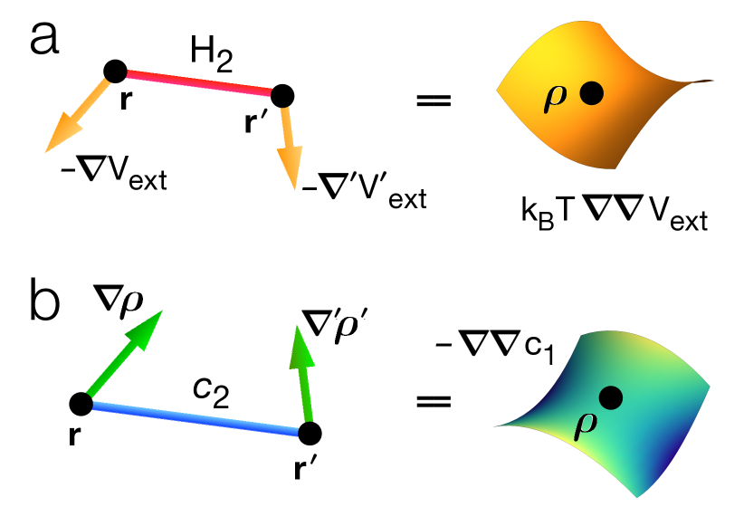
Figure 1: Illustrations of the sum rules for the variance of fluctuations. The sum rules arise from Noether invariance against spatial displacement. Shown are the different types of identical integrals. Thick dots indicate position variables that are integrated over. a External sum rule, Eq. (4), which relates the correlation function of density fluctuations $H_{2}({\mathbf{r}},{\mathbf{r}}^{\prime})$ and the external force field $-\nabla V_{\rm ext}({\mathbf{r}})$ with the product of the density profile $\rho({\mathbf{r}})$ and the Hessian of the external potential $k_{B}T\nabla\nabla V_{\rm ext}({\mathbf{r}}).$ This curvature is indicated by a schematic heat map. b Internal sum rule, Eq. (8), where the density gradient at two different positions is bonded by the direct correlation function $c_{2}({\mathbf{r}},{\mathbf{r}}^{\prime})$. This integral is identical to the integrated Hessian $-\nabla\nabla c_{1}({\mathbf{r}})$ (indicated by a schematic heat map) weighted by the local density $\rho({\mathbf{r}})$.

It is standard practice hansen2013 ; evans1979 ; evans1992 ; schmidt2022rmp to split off the trivial density covariance of the ideal gas and define the total correlation function $h({\mathbf{r}},{\mathbf{r}}^{\prime})$ via the identity $H_{2}({\mathbf{r}},{\mathbf{r}}^{\prime})=\rho({\mathbf{r}})\rho({\mathbf{r}}^{\prime})h({\mathbf{r}},{\mathbf{r}}^{\prime})+\rho({\mathbf{r}})\delta({\mathbf{r}}-{\mathbf{r}}^{\prime})$. Insertion of this relation into Eq. (4) and then moving the term with the delta function to the right hand side yields the following alternative form of the second order Noether sum rule:

$$\int d{\mathbf{r}}d{\mathbf{r}}^{\prime}\rho\rho^{\prime}h({\mathbf{r}},{\mathbf{r}}^{\prime})\nabla V_{\rm ext}\nabla^{\prime}V_{\rm ext}^{\prime}=$$

$$\qquad\int d{\mathbf{r}}\big{(}k_{B}T\nabla\nabla V_{\rm ext}-(\nabla V_{\rm ext})\nabla V_{\rm ext}\big{)}\rho,$$ (5)

where we have left away the position arguments of the density profile and of the external potential for clarity and the prime denotes dependence on ${\mathbf{r}}^{\prime}$. For the ideal gas $h({\mathbf{r}},{\mathbf{r}}^{\prime})=0$ and hence the left hand side of (5) vanishes. That the right hand side then also vanishes can be seen explicitly by inserting the generalized barometric law hansen2013 $\rho({\mathbf{r}})\propto\exp(-\beta(V_{\rm ext}({\mathbf{r}})-\mu))$ and either integrating by parts, or by alternatively observing that $-(k_{B}T)^{2}\int d{\mathbf{r}}\nabla\nabla\rho({\mathbf{r}})=0$ and inserting the barometric law therein.

The right hand side of (5) makes explicit the balancing of the external force variance with the mean potential curvature, as given by its averaged Hessian. For an interacting (non-ideal) system, $h({\mathbf{r}},{\mathbf{r}}^{\prime})$ is nonzero in general and the associated external force correlation contributions are accumulated by the expression on the left hand side of Eq. (5). For the special case of a harmonic trap, as represented by the external potential $V_{\rm ext}({\mathbf{r}})=\kappa{\mathbf{r}}^{2}/2$, with spring constant $\kappa$ and Hessian $\nabla\nabla V_{\rm ext}({\mathbf{r}})=\kappa{\mathbbm{1}}$, where ${\mathbbm{1}}$ denotes the unit matrix, the mean curvature can be obtained explicitly. The first term on the right hand side of the sum rule (5) then simply becomes $k_{B}T\langle N\rangle\kappa{\mathbbm{1}}$ upon integration. Notably, this result holds independently of the type of interparticle interactions, although the latter affect $h({\mathbf{r}},{\mathbf{r}}^{\prime})$ as is present on the left hand side of Eq. (5). The remaining (second) term on the right hand side of Eq. (5) turns into $-\kappa^{2}\int d{\mathbf{r}}\rho({\mathbf{r}}){\mathbf{r}}{\mathbf{r}}$, where the integral is the matrix of second spatial moments of the density profile. The alternative form $-\kappa^{2}\langle\sum_{i}{\mathbf{r}}_{i}{\mathbf{r}}_{i}\rangle$ is obtained upon expressing the density profile as the average of $\hat{\rho}({\mathbf{r}})$ and carrying out the integral over ${\mathbf{r}}$. Collecting all terms and dividing by $\kappa^{2}$ we obtain the sum rule (5) for the case of an interacting system inside of a harmonic trap as: $\int d{\mathbf{r}}d{\mathbf{r}}^{\prime}\rho({\mathbf{r}})\rho({\mathbf{r}}^{\prime})h({\mathbf{r}},{\mathbf{r}}^{\prime}){\mathbf{r}}{\mathbf{r}}^{\prime}=\int d{\mathbf{r}}\rho({\mathbf{r}})(k_{B}T\kappa^{-1}{\mathbbm{1}}-{\mathbf{r}}{\mathbf{r}})$.

Internal force variance. In light of the external force fluctuations, one might wonder whether the global interparticle force also fluctuates. The corresponding operator is the sum of all interparticle forces: $\hat{\bf F}_{\rm int}^{\rm o}\equiv-\sum_{i}\nabla_{i}u({\mathbf{r}}_{1},\ldots,{\mathbf{r}}_{N})=-\int d{\mathbf{r}}\sum\delta({\mathbf{r}}-{\mathbf{r}}_{i})\nabla_{i}u({\mathbf{r}}_{1},\ldots,{\mathbf{r}}^{N})$, where the integrand in the later expression (including the minus sign) is the position-resolved force density operator schmidt2022rmp . However, for each microstate $\hat{\bf F}_{\rm int}^{\rm o}=0$, as can be seen e.g. via the translation invariance of the interparticle potential hermann2021noether , which ultimately expresses Newton’s third law actio est reactio. Hence trivially the average vanishes, $\langle\hat{\bf F}_{\rm int}^{\rm o}\rangle=0$, as do all higher moments, $\langle\hat{\bf F}_{\rm int}^{\rm o}\hat{\bf F}_{\rm int}^{\rm o}\rangle=0$, as well as cross correlations, $\langle\hat{\bf F}_{\rm int}^{\rm o}\hat{\bf F}_{\rm ext}^{\rm o}\rangle=0$, etc. Thus the total internal force does not fluctuate. This holds beyond equilibrium, as the properties of the thermal average are not required in the argument. Identical reasoning can be applied to a nonequilibrium ensemble, where these identities hence continue to hold.

While these probabilistic correlators vanish, deeper inherent structure can be revealed by addressing direct correlations, as introduced by Ornstein and Zernike in 1914 in their treatment of critical opalescence and to great benefit exploited in modern liquid state theory hansen2013 . We use the framework of classical density functional theory evans1979 ; evans1992 ; hansen2013 , where the effect of the interparticle interactions is encapsulated in the intrinsic Helmholtz excess free energy $F_{\rm exc}[\rho]$ as a functional of the one-body density distribution $\rho({\mathbf{r}})$. As the excess free energy functional solely depends on the interparticle interactions, it necessarily is invariant against spatial displacements. In technical analogy to the previous case of the external force, we consider a displaced density profile $\rho({\mathbf{r}}+{\boldsymbol{\epsilon}})$ and Taylor expand the excess free energy functional up to second order in ${\boldsymbol{\epsilon}}$ as follows:

$$\beta F_{\rm exc}[\rho^{\boldsymbol{\epsilon}}] =\beta F_{\rm exc}[\rho]-\int d{\mathbf{r}}c_{1}({\mathbf{r}})\nabla\rho({\mathbf{r}})\cdot{\boldsymbol{\epsilon}}$$

$$\quad-\frac{1}{2}\int d{\mathbf{r}}c_{1}({\mathbf{r}})\nabla\nabla\rho({\mathbf{r}}):{\boldsymbol{\epsilon}}{\boldsymbol{\epsilon}}$$ (6)

$$\quad-\frac{1}{2}\int d{\mathbf{r}}d{\mathbf{r}}^{\prime}c_{2}({\mathbf{r}},{\mathbf{r}}^{\prime})\nabla\rho({\mathbf{r}})\nabla^{\prime}\rho({\mathbf{r}}^{\prime}):{\boldsymbol{\epsilon}}{\boldsymbol{\epsilon}},$$

where $\rho^{\boldsymbol{\epsilon}}({\mathbf{r}})=\rho({\mathbf{r}}+{\boldsymbol{\epsilon}})$ is again a shorthand. The one- and two-body direct correlation functions are given, respectively, via the functional derivatives $c_{1}({\mathbf{r}})=-\beta\delta F_{\rm exc}[\rho]/\delta\rho({\mathbf{r}})$ and $c_{2}({\mathbf{r}},{\mathbf{r}}^{\prime})=-\beta\delta^{2}F_{\rm exc}[\rho]/\delta\rho({\mathbf{r}})\delta\rho({\mathbf{r}}^{\prime})$. Noether invariance demands that $F_{\rm exc}[\rho^{\boldsymbol{\epsilon}}]=F_{\rm exc}[\rho]$ and hence both the linear and the quadratic contributions in the Taylor expansion (6) need to vanish, irrespective of the value of ${\boldsymbol{\epsilon}}$. This yields, respectively:

$$\int d{\mathbf{r}}c_{1}({\mathbf{r}})\nabla\rho({\mathbf{r}}) =0,$$ (7)

$$\int d{\mathbf{r}}d{\mathbf{r}}^{\prime}c_{2}({\mathbf{r}},{\mathbf{r}}^{\prime})\nabla\rho({\mathbf{r}})\nabla^{\prime}\rho({\mathbf{r}}^{\prime}) =-\int d{\mathbf{r}}\rho({\mathbf{r}})\nabla\nabla c_{1}({\mathbf{r}}),$$ (8)

where we have integrated by parts on the right hand side of (8). The first order sum rule (7) expresses the vanishing of the global internal force $\langle\hat{\bf F}_{\rm int}^{\rm o}\rangle=0$ hermann2021noether . This can be seen by integrating by parts, which yields the integrand in the form $-\rho({\mathbf{r}})\nabla c_{1}({\mathbf{r}})$, which is the internal force density scaled by $-k_{B}T$. In formal analogy to the probabilistic variance in Eq. (4), the second order sum rule (8) could be viewed as relating the “direct variance” of the density gradient (left hand side) to the mean gradient of the internal one-body force field in units of $k_{B}T$ (right hand side), which, equivalently, is the Hessian of the local intrinsic chemical potential $-k_{B}Tc_{1}({\mathbf{r}})$, see Fig. 1(b).

As a conceptual point concerning the derivations of Eqs. (7) and (8), we point out that the excess free energy density functional $F_{\rm exc}[\rho]$ is an intrinsic quantity, which does not explicitly depend on the external potential $V_{\rm ext}({\mathbf{r}})$. Hence there is no need to explicitly take into account a corresponding shift of $V_{\rm ext}({\mathbf{r}})$. This is true despite the fact that in an equilibrium situation one would consider the external potential (and the correspondingly generated external force field) as the physical reason for the (inhomogeneous) density profile to be stable. Both one-body fields are connected via the (Euler-Lagrange) minimization equation of density functional theory evans1979 ; evans1992 ; hansen2013 : $k_{B}T\ln\rho({\mathbf{r}})=k_{B}Tc_{1}({\mathbf{r}})-V_{\rm ext}({\mathbf{r}})+\mu$, where we have set the thermal de Broglie wavelength to unity. For given density profile, we can hence trivially obtain the corresponding external potential as $V_{\rm ext}({\mathbf{r}})=-k_{B}T\ln\rho({\mathbf{r}})+k_{B}Tc_{1}({\mathbf{r}})+\mu$, which makes the fundamental Mermin-Evans evans1979 ; hansen2013 ; evans1992 ; schmidt2022rmp map $\rho({\mathbf{r}})\to V_{\rm ext}({\mathbf{r}})$ explicit.

As a consistency check, the second order sum rules (4) and (8) can alternatively be derived from the hyper virial theorm hirschfelder1960 ; haile1992 or from spatially resolved correlation identities hermann2021noether ; baus1984 . Following the latter route, one starts with $\int d{\mathbf{r}}^{\prime}H_{2}({\mathbf{r}},{\mathbf{r}}^{\prime})\nabla^{\prime}V_{\rm ext}({\mathbf{r}}^{\prime})=-k_{B}T\nabla\rho({\mathbf{r}})$ and $\int d{\mathbf{r}}^{\prime}c_{2}({\mathbf{r}},{\mathbf{r}}^{\prime})\nabla^{\prime}\rho({\mathbf{r}}^{\prime})=\nabla c_{1}({\mathbf{r}})$, respectively. The derivation the requires the choice of a suitable field as a multiplier ($\nabla V_{\rm ext}({\mathbf{r}})$ and $\nabla\rho({\mathbf{r}})$, respectively), spatial integration over the free position variable, and subsequent integration by parts. However, this strategy i) requires the correct choice for multiplication to be made, and ii) it does not allow to identify the Noether invariance as the underlying reason for the validity. In contrast, the Nother route is constructive and it allows to trace spatial invariance as the fundamental physical reason for the respective identity to hold.

Thermal diffusion force variance. Similar to the treatment of the excess free energy functional, one can shift and expand the ideal free energy functional $F_{\rm id}[\rho]=k_{B}T\int d{\mathbf{r}}\rho({\mathbf{r}})(\ln\rho({\mathbf{r}})-1)$. Exploiting the translational invariance at first order leads to vanishing of the total diffusive force: $-k_{B}T\int d{\mathbf{r}}\nabla\rho({\mathbf{r}})=0$, and at second order: $\int d{\mathbf{r}}\rho({\mathbf{r}})^{-1}(\nabla\rho({\mathbf{r}}))\nabla\rho({\mathbf{r}})=-\int d{\mathbf{r}}\rho({\mathbf{r}})\nabla\nabla\ln\rho({\mathbf{r}})$. These ideal identities can be straightforwardly verified via integration by parts (boundary contributions vanish) and they complement the excess results (7) and (8).

Outlook. While we have restricted ourselves throughout to translations in equilibrium, the variance considerations apply analogously for rotational invariance hermann2021noether and to the dynamics, where invariance of the power functional forms the basis hermann2021noether ; schmidt2022rmp . In future work it it would be highly interesting to explore connections of our results to statistical thermodynamics seifert2012 , to the study of liquids under shear asheichyk2021 , to the large fluctuation functional jack2015 , as well as to recent progress in systematically incorporating two-body correlations into classical density functional theory tschopp2020 ; tschopp2021 . Investigating the implications of our variance results for Levy-noise yuvan2022 is interesting. As the displacement vector ${\boldsymbol{\epsilon}}$ is arbitrary both in its orientation and its magnitude our reasoning does not stop at second order in the Taylor expansion, see Eqs. (2) and (6). Assuming that the power series exists, the invariance against the displacement rather implies that each order vanishes individually, which gives rise to a hierarchy of correlation identities of third, fourth, etc. moments that are interrelated with third, fourth, etc. derivatives of the external potential (when starting from $\Omega[V_{\rm ext}]$) or the one-body direct correlation function (when starting from the excess free energy density functional $F_{\rm exc}[\rho]$).

Future use of the sum rules can be manifold, ranging from the construction and testing of new theories, such as approximate free energy functionals within the classical density functional framework, to validation of simulation data (to ascertain both correct implementation and sufficient equilibration and sampling) and numerical theoretical results. To give a concrete example, in systems like the confined hard sphere liquid considered by Tschopp et al. tschopp2022forceDFT on the basis of fundamental measure theory, one could apply and test the sum rule (5) explicitly, as the inhomogeneous total pair correlation function $h({\mathbf{r}},{\mathbf{r}}^{\prime})$ is directly accessible in the therein proposed force-DFT approach.

Data availability
Data sharing is not applicable to this study as no datasets were generated or analyzed during the current study.

Acknowledgments
Open Access funding enabled and organized by Projekt DEAL. We thank Daniel de las Heras, Thomas Fischer, and Gerhard Jung for useful discussions.

Author contributions
S.H. and M.S. have jointly carried out the work and written the paper.

Competing interests
The authors declare no competing interests.

References

- (1) E. Noether, Invariante Variationsprobleme, Nachr. d. König. Gesellsch. d. Wiss. zu Göttingen, Math.-Phys. Klasse, 235 (1918). English translation by M. A. Tavel: Invariant variation problems, Transp. Theo. Stat. Phys. 1, 186 (1971); for a version in modern typesetting see: Frank Y. Wang, arXiv:physics/0503066v3 (2018).
- (2) N. Byers, E. Noether’s discovery of the deep connection between symmetries and conservation laws, arXiv:physics/9807044 (1998).
- (3) F. Turci and N. B. Wilding, Phase separation and multibody effects in three-dimensional active Brownian particles, Phys. Rev. Lett. 126, 038002 (2021).
- (4) F. Turci and N. B. Wilding, Wetting transition of active Brownian particles on a thin membrane, Phys. Rev. Lett. 127, 238002 (2021).
- (5) M. K. Coe, R. Evans, and N. B. Wilding, Density depletion and enhanced fluctuations in water near hydrophobic solutes: identifying the underlying physics, Phys. Rev. Lett. 128, 045501 (2022).
- (6) A. L. Thorneywork, S. K. Schnyder, D. G. A. L. Aarts, J. Horbach, R. Roth, and R. P. A. Dullens, Structure factors in a two-dimensional binary colloidal hard sphere system, Mol. Phys. 116, 3245 (2018).
- (7) F. Höfling and S. Dietrich, Enhanced wavelength-dependent surface tension of liquid-vapour interfaces, Europhys. Lett. 109, 46002 (2015).
- (8) A. O. Parry, C Rascón, and R. Evans, The local structure factor near an interface; beyond extended capillary-wave models, J. Phys.: Condens. Matter 28, 244013 (2016).
- (9) P. I. Hurtado, C. Pérez-Espigares, J. J. del Pozo, and P. L. Garrido, Symmetries in fluctuations far from equilibrium, Proc. Natl. Acad. Sci. 108, 7704 (2011).
- (10) D. Lacoste and P. Gaspard, Isometric fluctuation relations for equilibrium states with broken symmetry, Phys. Rev. Lett. 113, 240602 (2014).
- (11) D. Lacoste and P. Gaspard, Fluctuation relations for equilibrium states with broken discrete or continuous symmetries, J. Stat. Mech. 2015, P11018 (2015).
- (12) A. Dechant and S. Sasa, Fluctuation-response inequality out of equilibrium, Proc. Natl. Acad. Sci. 117, 6430 (2020).
- (13) U. Seifert, Stochastic thermodynamics, fluctuation theorems and molecular machines, Rep. Prog. Phys. 75, 126001 (2012).
- (14) A. G. Lezcano and A. C. M. de Oca, A stochastic version of the Noether theorem, Found. Phys. 48, 726 (2018).
- (15) J. C. Baez and B. Fong, A Noether theorem for Markov processes, J. Math. Phys. 54, 013301 (2013).
- (16) I. Marvian and R. W. Spekkens, Extending Noether’s theorem by quantifying the asymmetry of quantum states, Nat. Commun. 5, 3821 (2014).
- (17) S. Sasa and Y. Yokokura, Thermodynamic entropy as a Noether invariant, Phys. Rev. Lett. 116, 140601 (2016).
- (18) Y. Minami and S. Sasa, Thermodynamic entropy as a Noether invariant in a Langevin equation, J. Stat. Mech. 2020 013213 (2020).
- (19) S. Sasa, S. Sugiura, and Y. Yokokura, Thermodynamical path integral and emergent symmetry, Phys. Rev. E 99, 022109 (2019).
- (20) M. Revzen, Functional integrals in statistical physics, Am. J. Phys. 38, 611 (1970).
- (21) J. C. Baez, Getting to the Bottom of Noether’s Theorem, arXiv:2006.14741 (2022).
- (22) S. Hermann and M. Schmidt, Noether’s Theorem in Statistical Mechanics, Commun. Phys. 4, 176 (2021).
- (23) S. Hermann and M. Schmidt, Why Noether’s Theorem applies to Statistical Mechanics, J. Phys.: Condens. Matter 34, 213001 (2022) (invited Topical Review).
- (24) S. M. Tschopp, F. Sammüller, S. Hermann, M. Schmidt, and J. M. Brader, Force density functional theory for fluids in- and out-of-equilibrium, Phys. Rev. E 106, 014115 (2022).
- (25) M. Baus, Broken symmetry and invariance properties of classical fluids, Mol. Phys. 51, 211 (1984).
- (26) J.-P. Hansen and I. R. McDonald, Theory of Simple Liquids, 4th ed. (Academic Press, London, 2013).
- (27) R. Evans, The nature of the liquid-vapour interface and other topics in the statistical mechanics of non-uniform, classical fluids, Adv. Phys. 28, 143 (1979).
- (28) R. Evans, Density functionals in the theory nonuniform fluids, in: Fundamentals of Inhomogeneous Fluids, edited by D. Henderson (Dekker, New York, 1992).
- (29) M. Schmidt, Power functional theory for many-body dynamics, Rev. Mod. Phys. 94, 015007 (2022).
- (30) J. O. Hirschfelder, Classical and Quantum Mechanical Hypervirial Theorems, J. Chem. Phys. 33, 1462 (1960).
- (31) J. M. Haile, Molecular Dynamics Simulation: Elementary Methods, (Wiley, New York, 1992).
- (32) K. Asheichyk, M. Fuchs, and M. Krüger, Brownian systems perturbed by mild shear: comparing response relations, J. Phys.: Condens. Matter 33, 405101 (2021).
- (33) R. L. Jack and P. Sollich, Effective interactions and large deviations in stochastic processes, Eur. Phys. J. Special Topics 224, 2351 (2015).
- (34) S. M. Tschopp, H. D. Vuijk, A. Sharma, and J. M. Brader, Mean-field theory of inhomogeneous fluids, Phys. Rev. E 102, 042140 (2020).
- (35) S. M. Tschopp and J. M. Brader, Fundamental measure theory of inhomogeneous two-body correlation functions, Phys. Rev. E 103, 042103 (2021).
-
(36)
S. Yuvan and M. Bier,
Accumulation of particles and formation of a dissipative structure in
a nonequilibrium bath,
Entropy 24, 189 (2022).