Adaptive Hermite spectral methods in unbounded domains

Abstract

Recently, new adaptive techniques were developed that greatly improved the efficiency of solving PDEs using spectral methods. These adaptive spectral techniques are especially suited for accurately solving problems in unbounded domains and require the monitoring and dynamic adjustment of three key tunable parameters: the scaling factor, the displacement of the basis functions, and the spectral expansion order. There have been few analyses of numerical methods for unbounded domain problems. Specifically, there is no analysis of adaptive spectral methods to provide insight into how to increase efficiency and accuracy through dynamical adjustment of parameters. In this paper, we perform the first numerical analysis of the adaptive spectral method using generalized Hermite functions in both one- and multi-dimensional problems. Our analysis reveals why adaptive spectral methods work well when a “frequency indicator” of the numerical solution is controlled. We then investigate how the implementation of the adaptive spectral methods affects numerical results, thereby providing guidelines for the proper tuning of parameters. Finally, we further improve performance by extending the adaptive methods to allow bidirectional basis function translation, and the prospect of carrying out similar numerical analysis to solving PDEs arising from realistic difficult-to-solve unbounded models with adaptive spectral methods is also briefly discussed.

1 Introduction

Unbounded domain problems require efficient numerical methods for computation. For example, resolving the decay of the solution of Schrödinger’s equations at infinity requires efficient unbounded domain algorithms [14]. In population dynamics, tracking cell volume blowup in structured population PDE models demands high-accuracy numerical methods in unbounded domains [15, 12]. Furthermore, in solid-state physics, numerical methods for unbounded domains are required for studying long-range particle interactions [16, 17]. Despite these numerous applications, there has been little research on developing efficient and accurate algorithms for solving models in unbounded domains.

Adaptive methods, such as re-defining grids for finite difference methods [10] and re-generating meshes for finite element methods [23, 8, 11, 9], which are applied to PDEs defined on finite domains, can dramatically improve not only accuracy but computational efficiency. Recently, novel adaptive techniques for spectral methods have been developed and incorporated into efficient algorithms for numerically solving PDEs in unbounded domains that posed substantial numerical difficulties when using previous numerical methods [3, 4]. The adaptive spectral methods consist of three separate but interdependent procedures: (i) a scaling technique that adjusts the shape of the basis functions to capture the varying decay rate of the function at infinity, (ii) a moving technique that adjusts the displacement of the basis function to better assign allocation points and capture intrinsic translation of the solution, and (iii) a $p$-adaptive technique that adjusts the expansion order of the numerical solution to deal with oscillations of the solution. These adaptive spectral techniques require tuning of three key parameters: the scaling factor $\beta$, the displacement of the basis function $x_{0}$, and the spectral expansion order $N$. For example, if we use the generalized Hermite functions [24] as basis functions on $\mathbb{R}$, the variables $\beta,x_{0}$, and $N$ appear in a spectral expansion according to

$$U_{N,x_{0}}^{\beta}\coloneqq\sum_{i=0}^{N}u_{i,x_{0}}^{\beta}\hat{\mathcal{H}}_{i}^{\beta}(x-x_{0})=\sum_{i=0}^{N}u_{i,x_{0}}^{\beta}\hat{\mathcal{H}}_{i}(\beta(x-x_{0})),$$ (1)

where $u_{i,x_{0}}^{\beta}$ is the coefficient of the $i^{\rm th}$-order generalized Hermite function $\hat{\mathcal{H}}_{i}^{\beta}$

$$\hat{\mathcal{H}}_{i}^{\beta}\coloneqq\frac{1}{\sqrt{2^{i}i!}}H_{i}(\beta x)e^{-\tfrac{(\beta{x})^{2}}{2}},\,\,\,H_{i}(x)=(-1)^{i}e^{x^{2}}\partial_{x}^{i}(e^{-x^{2}}).$$ (2)

For example, for PDEs involving a spatial variable $x\in\mathbb{R}$ and a temporal variable $t\in[0,T]$, we typically impose a spectral expansion using generalized Hermite functions of $x$ and forward time $t$ starting from an initial condition at $t=0$.

Adaptive spectral techniques are implemented as shown in Fig. 1. Specifically, the algorithm changes the displacement of the basis function $x_{0}$ to control an exterior-error indicator $\mathcal{E}(U_{N,x_{0}}^{\beta})$ that reflects the ratio of the numerical solution’s error outside a given domain to the error in the whole domain. It also changes the scaling factor $\beta$ as well as the spectral expansion order $N$ to control a frequency indicator $\mathcal{F}(U_{N,x_{0}}^{\beta})$ that measures the spread and oscillation of the solution. The indicators are defined in [3] as

$$\mathcal{E}(U_{N,x_{0}}^{\beta})=\frac{\|\partial_{x}U_{N,x_{0}}^{\beta}\cdot\mathbb{I}_{(x_{R},\infty)}\|}{\|\partial_{x}U_{N,x_{0}}^{\beta}\cdot\mathbb{I}_{(-\infty,+\infty)}\|},$$ (3)

where $x_{R}=x_{[\frac{2N+2}{3}]}^{\beta}$ is the $[\frac{2N+2}{3}]^{\text{th}}$ collocation point of the generalized, $x_{0}$-shifted Hermite functions, and

$$\mathcal{F}(U_{N,x_{0}}^{\beta})=\frac{\|(I-\pi_{N-M,x_{0}}^{\beta})U_{N,x_{0}}^{\beta}(\cdot,t)\|}{\|U_{N,x_{0}}^{\beta}(\cdot,t)\|},$$ (4)

with $M$ is taken to be $[\frac{N}{3}]$.

Figure 1: Flow chart of an adaptive Hermite spectral method equipped with scaling, moving, and $p$-adaptive techniques. $x_{0}$ and $\tilde{x}_{0}$ are the displacements before and after the moving technique is used, and $\tilde{x}_{0}$ is chosen such that the exterior-error indicator $\mathcal{E}(U^{\beta}_{\tilde{x}_{0},N})$ is below a moving threshold $\mathcal{E}_{\text{thres}}$. $\beta$ and $\tilde{\beta}$ are the scaling factors before and after scaling when the scaling technique is used, where the scaling factor $\tilde{\beta}$ is chosen such that $\mathcal{F}(U^{\tilde{\beta}}_{x_{0},N})$ is below a scaling threshold $\mathcal{F}^{s}_{\text{thres}}$. $N$ and $\tilde{N}$ are the expansion orders before and after adjusting the expansion order when the $p$-adaptive technique is used. $\tilde{N}$ is chosen such that $\mathcal{F}(U^{\beta}_{x_{0},\tilde{N}})$ is below a $p$-adaptivity threshold $\mathcal{F}^{p}_{\text{thres}}$. The three thresholds $\mathcal{E}_{\text{thres}},\mathcal{F}^{s}_{\text{thres}}$, and $\mathcal{F}^{p}_{\text{thres}}$ are updated dynamically as time progresses. Details are described in [3, 4]. In addition, we impose constraints on the maximum allowable displacement $d_{\max}$ and expansion order increment $N_{\max}$ within a single step, and the minimum and maximum scaling factors $\underline{\beta}$ and $\overline{\beta}$.

The major advantage of the proposed adaptive spectral method Fig. 1 is that it depends only on the numerical solution $U^{\beta}_{N,x_{0}}$ and thus does not require any prior knowledge on how the solution will evolve. This feature is similar to that of the adaptive mesh generating method which also only depends on the numerical solution [25]. However, unlike the posterior error indicator that is usually used in finite element methods [21], the exterior-error and frequency indicators used in our adaptive spectral method does not directly furnish the error. The exterior-error indicator is specifically designed for spectral methods in unbounded domain problems, and controlling it by properly translating the basis functions can lead to a better approximation at infinity. On the other hand, the frequency indicator applies to spectral methods in both bounded and unbounded domains, and more resembles a measure of the numerical error. Ultimately, the adaptive spectral method aims at controlling the error by maintaining a small frequency indicator. While adjusting the scaling factor or changing the expansion order directly controls the frequency indicator, changing the displacement of the basis functions to control the exterior-error indicator also helps control the frequency indicator, as was shown in [3].

Despite the numerical success of adaptive spectral methods when applied on unbounded domains, there exists no theoretical analysis of how the parameters $\beta,x_{0}$, and $N$ affect the algorithm’s performance and thus far no general rule on how to best adjust these parameters in the moving ($x_{0}\leftarrow\tilde{x}_{0}$), scaling ($\beta\leftarrow\tilde{\beta}$), and expansion order adjustment ($N\leftarrow\tilde{N}$) subroutines in order to minimize errors. Since the improper adjustment of $\beta,x_{0}$, and $N$ can lead to large errors [22, 18], properly choosing them is crucial for the effective implementation of adaptive spectral methods.

symbol	definition
$\hat{\mathcal{H}}_{i,x_{0}}^{\beta}$	generalized $i^{\rm th}$-order Hermite function with a scaling factor $\beta$ and displacement $x_{0}$, defined in $\mathbb{R}$ as $\hat{\mathcal{H}}_{i,x_{0}}^{\beta}\coloneqq\hat{\mathcal{H}}_{i}(\beta(x-x_{0}))$
$P_{N,x_{0}}^{\beta}$	function space $P_{N}^{x_{0},\beta}\coloneqq\{\hat{\mathcal{H}}_{i,x_{0}}^{\beta}\}_{i=0}^{N}$
$I$	the identity operator
$\pi_{N,x_{0}}^{\beta}$	the projection operator $\pi_{N,x_{0}}^{\beta}$ $:L^{2}(\mathbb{R})\rightarrow P_{N}^{x_{0},\beta}$ such that $(\pi_{N}^{x_{0},\beta}u(x)$, $u(x)-\pi_{N}^{x_{0},\beta}u(x))=0$
$\mathcal{I}_{N,x_{0}}^{\beta}$	the interpolation operator $\mathcal{I}_{N,x_{0}}^{\beta}$ $:L^{2}(\mathbb{R})\rightarrow P_{N}^{x_{0},\beta}$ such that $\mathcal{I}_{N}^{x_{0},\beta}u(x_{i})=u(x_{i})$ where $\{x_{i}^{N}\}_{i=0}^{N}$ are collocation points of $\{\hat{\mathcal{H}}_{i,x_{0}}^{\beta}\}_{i=0}^{N}$
$U_{N,x_{0}}^{\beta}$	spectral expansion $U_{N,x_{0}}^{\beta}=\sum_{i=0}^{N}u_{i,x_{0}}^{\beta}\hat{\mathcal{H}}_{i}(\beta(x-x_{0}))$
$N$	expansion order of the spectral expansion
$\beta$	scaling factor of the generalized Hermite functions
$x_{0}$	displacement of the generalized Hermite functions
$\mathcal{E}_{R}(U_{N,x_{0}}^{\beta}),\mathcal{E}_{L}(U_{N,x_{0}}^{\beta})$	$\mathcal{E}_{R}$: the right exterior-error indicator of the spectral expansion $U_{N,x_{0}}^{\beta}$;                 $\mathcal{E}_{L}$: the left exterior-error indicator of the spectral expansion $U_{N,x_{0}}^{\beta}$
$\mathcal{F}(U_{N,x_{0}}^{\beta})$	frequency indicator for the spectral expansion $U_{N,x_{0}}^{\beta}$
$q$	scaling factor update ($\beta$ to $\tilde{\beta}$) ratio ($\tilde{\beta}\leftarrow q^{n}\beta~{}\text{or}~{}q^{-n}\beta,n\in\mathbb{N}^{+}$) in the scaling technique
$\nu$	threshold for activating the scaling technique
$\delta$	minimal displacement of updating the displacement $x_{0}$ to $\tilde{x}_{0}$ ($\tilde{x}_{0}\leftarrow x_{0}+nx_{0}~{}\text{or}~{}x_{0}-nx_{0},n\in\mathbb{N}^{+}$) in the moving technique
$\mu$	threshold for activating the moving technique
$\eta$	threshold for increasing the number of basis functions
$\eta_{0}$	threshold for decreasing the number of basis functions
$\gamma$	post-refinement adjustment factor for refinement threshold $\tilde{\eta}\leftarrow\gamma\eta$
$L^{2}(a,b;V)$	space of functions $\{f:[a,b]\rightarrow{V}$ ($V$ is a Banach space) such that $f$ is measurable for $\mbox{d}{t}~{}\text{and}~{}\int_{a}^{b}f(t)^{2}\mbox{d}{t}<\infty\}$
$X(t_{1},t_{2})$	function space $\{f:f(x,s)\in L^{2}((t_{1},t_{2}),t;H^{1}(\mathbb{R})),\partial_{s}f(x,s)\in L^{2}((t_{1},t_{2}),$ $t;H^{1}(\mathbb{R}))\}$
$e(t)$	$L^{2}$-norm of the error $\|u(\cdot,t)-U_{N,x_{0}}^{\beta}(\cdot,t)\|_{L^{2}}$ at time $t$

Table 1: Overview of variables and notation. List of the main variables and notations associated with the overall adaptive spectral method. Three key variables for adaptive spectral methods with generalized Hermite functions are the scaling factor $\beta$ that determines the shape of the basis functions, the displacement of the basis functions $x_{0}$, and the expansion order $N$ of the spectral decomposition.

In this paper, we carry out a numerical analysis of the adaptive spectral method to specify how algorithm parameters affect the accuracy of numerical results. We restrict ourselves to a parabolic model problem, in any dimension, and use generalized Hermite functions as basis functions to explore numerical performances and how parameters in the adaptive spectral algorithm control the tuning of the three key quantities $\beta,x_{0}$, and $N$ in Fig. 1. Furthermore, we will explicitly show how the frequency indicator is related to the lower error bound, justifying the maintenance of a small frequency indicator in the adaptive spectral algorithm.

Depending on the inverse inequality for generalized Hermite functions [2], such analyses for numerically solving unbounded-domain PDEs provide a posterior error estimate. This error estimate only relies on the numerical solution and the adjustment of $\beta,x_{0}$, and $N$. Our main result is

Theorem 1.

The $L^{2}$-error at time $T$ when solving a parabolic PDE in $(x,t)\in\mathbb{R}\times[0,T]$ with the generalized Hermite functions and using adaptive techniques is bounded by

$$e(T)\coloneqq\|u(\cdot,T)-U_{N,x_{0}}^{\beta}(\cdot,T)\|_{2}\leq e_{0}+e_{\text{S}}+e_{\text{M}}+e_{\text{C}},$$ (5)

where $U_{N,x_{0}}^{\beta}$ is the numerical solution; $e_{0}$ is the numerical discretization error from numerically solving the PDE. $e_{\text{S}}$ is the error bound arising from changing the scaling factor from $\beta$ to $\tilde{\beta}$; $e_{\text{M}}$ is the error bound for changing the displacement from $x_{0}$ to $\tilde{x}_{0}$; $e_{\text{C}}$ is the error bound for coarsening, i.e., reducing the expansion order from $N$ to $\tilde{N}$. More specifically, $e_{\text{S}},e_{\text{M}}$, and $e_{\text{C}}$ take the forms

$$e_{\text{S}} \coloneqq\sum\limits_{\rm scale}\frac{|\tilde{\beta}-\beta|\sqrt{1+\tfrac{\tilde{\beta}}{\beta}}}{\sqrt{2}\tilde{\beta}}\|x\partial_{x}U_{N,x_{0}}^{\beta}(\cdot,t)\|_{2},$$ (6)

$$e_{\text{M}} \coloneqq\sum\limits_{\rm move}|x_{0}-\tilde{x}_{0}|\|\partial_{x}U_{N,x_{0}}^{\beta}(\cdot,t)\|_{2},$$

$$e_{\text{C}} \coloneqq\sum\limits_{\rm coarsen}\|(I-\pi_{\tilde{N},x_{0}}^{\beta})U_{N,x_{0}}^{\beta}(\cdot,t)\|_{2},$$

where the sum $\sum\limits_{\rm scale}$ is taken over all scaling steps, the sum $\sum\limits_{\rm move}$ is taken over all moving steps, and $\sum\limits_{\rm coarsen}$ is taken over all coarsening steps. The operators $I$ and $\pi_{\tilde{N},x_{0}}^{\beta}$ are defined in Table 1.

This result allows us to provide general guidelines for selecting the parameters in the adaptive spectral algorithm that lead to the proper tuning of $\beta,x_{0}$, and $N$. Specifically, the numerical discretization error $e_{0}$ in Eq. (5) we aim to minimize depends on $\beta,x_{0},N$. The precise dependences will be given in Section 2. Since the adaptive techniques depend only on the numerical solution and do not require any prior knowledge of the solution, the last three terms in Eq. (5) depend only on the numerical solution. From this theorem, we can conclude that the smaller the adjustment in the scaling factor or in the displacement of the basis functions, the smaller the error bounds $e_{\text{S}},e_{\text{M}}$ for carrying out the adaptive techniques. However, given that improper $\beta$ or $x_{0}$ leads to very large $e_{0}$, proper dynamic adjustment of $\beta$ and $x_{0}$ are still needed to keep $e_{0}$ small, possibly at the expense of accumulating more error in $e_{\text{S}},e_{\text{M}}$.

In Fig. 1, the threshold $\mathcal{E}^{m}_{\text{thres}}$ is chosen to be the exterior-error indicator evaluated after the last adjustment of the displacement $x_{0}$, multiplied by a constant $\mu>1$. As shown in [3], if the exterior-error indicator grows above such a threshold, the function is moving rightward, indicating that we should replace $x_{0}$ with $\tilde{x}_{0}>x_{0}$. As $\lim\limits_{\tilde{x}_{0}\rightarrow\infty}\mathcal{E}(U_{N,x_{0}}^{\beta}(x+\tilde{x}-x_{0},t))=0$, we can always find a $\tilde{x}_{0}$ such that $\mathcal{E}(U_{N,x_{0}}^{\beta}(x+\tilde{x}-x_{0},t))<\mathcal{E}^{m}_{\text{thres}}$ and renew $x_{0}\leftarrow\min\{\tilde{x}_{0},x_{0}+d_{\max}\}$. By the form of $e_{\text{M}}$ in Eq. (6), we can conclude that finding the smallest $\tilde{x}_{0}$ such that $\mathcal{E}(U_{N,x_{0}}^{\beta}(x+\tilde{x}-x_{0},t))<\mathcal{E}^{m}_{\text{thres}}$ while keeping $x_{0}-\tilde{x}_{0}$ small can effectively reduce $e_{\text{M}}$.

The scaling technique and the $p$-adaptive techniques are directly coupled with each other as they rely on monitoring the same frequency indicator. If the function decays more slowly at infinity, then the frequency indicator is likely to increase, whereas if the function decays faster, the frequency indicator is likely to decrease. When $\beta$ is to be decreased (more slowly decaying function), the threshold $\mathcal{F}^{s}_{\text{thres}}$ is chosen to be the frequency indicator after the last scaling or change of expansion order, multiplied by a constant $\nu>1$. When $\beta$ is to be increased (faster decaying function), we set the threshold to be the frequency indicator after the last scaling or expansion order change since a function that decreases more slowly is harder to approximate requiring us to be more tolerant of an increase in the frequency indicator. The explicit form of $e_{\text{S}}$ in Eq. (6) suggests that to reduce $e_{\text{S}}$, it is desirable to find a $\tilde{\beta}$ such that $\tilde{\beta}-\beta$ is small. However, there is no guarantee that one can find a $\tilde{\beta}$ such that $\mathcal{F}(U_{N,x_{0}}^{\tilde{\beta}})<\mathcal{F}^{s}_{\text{thres}}$. If the frequency indicator cannot be suppressed below the threshold by choosing $\tilde{\beta}$, a probable cause is that the function becomes more oscillatory, implying that the expansion order should be adjusted.

The $p$-adaptive threshold $\mathcal{F}^{p}_{\text{thres}}$ is chosen to be the frequency indicator after the last adjustment of expansion order, multiplied by a constant $\eta>1$ if refinement is required. Alternatively, if coarsening is required, the threshold is chosen to be the frequency indicator after the last change of expansion order, multiplied by an another constant $\eta_{0}>1$ but $\eta_{0}<\eta$. $\eta$ is allowed to increase with time as functions that oscillate rapidly are harder to approximate, requiring us to be more tolerant of increases in the frequency indicator. Since $\lim\limits_{\tilde{N}\rightarrow\infty}\mathcal{F}(U_{\tilde{N},x_{0}}^{\beta}(x,t))=0$, we could always find a $\tilde{N}$ such that $\mathcal{F}(U_{\tilde{N},x_{0}}^{\beta}(x,t))\leq\mathcal{F}^{p}_{\text{thres}}$ if refinement is needed. By maintaining the scaling factor below the $p$-adaptive threshold $\mathcal{F}^{p}_{\text{thres}}$ and using the relationship between the error and the frequency indicator, the lower error bound can be shown to be always smaller than $\mathcal{F}^{p}_{\text{thres}}\|u(\cdot,t)\|_{2}-\|(I-\pi_{N-M,x_{0}}^{\beta})u(\cdot,t)\|_{2}$, where $u$ is the analytical solution. However, tradeoffs arise. For example, refinement itself does not bring about an additional error, but could result in additional computational cost. On the other hand, if coarsening is implemented, a smaller $\tilde{N}$ could lead to a larger error $e_{\text{C}}$ in Eq. (6) but also result in smaller computational cost.

In the next section, we formulate the model problem using generalized Hermite functions and perform numerical analysis. In Section 3, numerical analysis for applying the adaptive techniques is carried out and Theorem 1 is proved. Furthermore, the relationship between the error and the frequency indicator is analyzed, explicitly explaining the efficacy of the algorithm shown in Fig. 1. In Section 4, numerical experiments are carried out, and an additional improvement of the adaptive spectral method in the moving technique is proposed and discussed. For completeness, we list the common variables and notations in Table 1 that we use throughout this paper.

2 Errors in solving a model problem with generalized Hermite functions

In this section, we first formulate a parabolic equation in weak form [1]:

$$\big{(}\partial_{t}u(\cdot,t),v(\cdot))+a\big{(}u(x,t),v(x);t\big{)} =\big{(}f(\cdot,t),v(\cdot)\big{)},\,\,\,x\in\mathbb{R},t\in[0,T],\,\,~{}\forall v(x)\in H^{1}(\mathbb{R}),$$ (7)

$$\big{(}u(\cdot,0),\tilde{v}(\cdot)\big{)} =\big{(}u_{0}(\cdot),\tilde{v}(\cdot)\big{)},\,\,\,\forall v(x)\in H^{1}(\mathbb{R}),$$ (8)

where $u_{0}(x)\in L^{2}(\mathbb{R})$ is the initial condition, $f(x,t)$ is the inhomogeneous source term (e.g. heat source in the heat equation), and $a(\cdot,\cdot;t)$ is a coercive symmetric bilinear form such that there exist constants $0<c_{0}<C_{0}$ satisfying

$$|a(u(x,t),v(x);t)|\leq C_{0}\|u(\cdot,t)\|_{H^{1}}\,\|v(\cdot)\|_{H^{1}}\quad\text{and}\quad c_{0}\|v(\cdot)\|_{H^{1}}^{2}\leq a(v,v;t),\,\,\,\forall u(\cdot,t),v(\cdot)\in H^{1}(\mathbb{R}).$$ (9)

In Eqs. (7), (8), and (9) and hereafter, the inner product is taken over the spatial variable $x$, and the norm $\|\cdot\|$ denotes the $L^{2}$-norm taken over $x$ unless otherwise specified.

The solution to the model problem, Eqs. (7) and (8), exists and is unique [20], and the solution $u$ is in the so-called Bochner-Sobolev space

$$W\left(0,t;H^{1}(\mathbb{R}),H^{-1}(\mathbb{R})\right)\coloneqq\big{\{}u:u(x,s)\in L^{2}\left(0,t;H^{1}(\mathbb{R})\right),\partial_{s}u(x,s)\in L^{2}\left(0,t;H^{-1}(\mathbb{R})\right)\big{\}}$$ (10)

where $H^{-1}(\mathbb{R})$ is the dual space of $H^{1}(\mathbb{R})$. For simplicity, we assume that $f(x,t)\in C(\mathbb{R}\times[0,t]),\partial_{s}u(x,s)\in L^{2}(0,t;H^{1}(\mathbb{R}))$ and therefore $u\in X(0,t)$, and its norm is given by

$$\|u\|_{X(0,t)}^{2}=\int_{0}^{t}\Big{(}\|u(\cdot,s)\|^{2}_{H^{1}(\mathbb{R})}+\|\partial_{s}u(\cdot,s)\|^{2}_{H^{1}(\mathbb{R})}\Big{)}\mbox{d}{s}+\|u(\cdot,0)\|^{2}.$$ (11)

Analysis of finite element methods for solving Eqs. (7) and (8) for bounded $x$ has already been performed [19]. Here, we wish to numerically solve Eqs. (7) and (8) using spectral methods with generalized Hermite functions. We first fix the scaling factor $\beta$, the displacement $x_{0}$ of the basis functions $\hat{\mathcal{H}}_{i,x_{0}}^{\beta}$, and the expansion order $N$ of the trial and test functions. Integrating Eq. (7) w.r.t time, we wish to find a $U_{N,x_{0}}^{\beta}(x,s)\in L^{2}(0,t;P_{N,x_{0}}^{\beta}(\mathbb{R}))$ such that for any test function $v_{N,x_{0}}^{\beta}(x,t)\in L^{2}(0,t;P_{N,x_{0}}^{\beta}(\mathbb{R}))$ and $\tilde{v}_{N,x_{0}}^{\beta}\in P_{N,x_{0}}^{\beta}(\mathbb{R})$,

$$\int_{0}^{t}\left[\big{(}\partial_{s}U_{N,x_{0}}^{\beta},v_{N,x_{0}}^{\beta}\big{)}+a\big{(}U_{N,x_{0}}^{\beta},v_{N,x_{0}}^{\beta};t\big{)}\right]\mbox{d}{s}+\big{(}U_{N,x_{0}}^{\beta}(\cdot,0),\tilde{v}_{N,x_{0}}^{\beta}(\cdot)\big{)}$$ (12)

$$\hskip 91.04872pt=\int_{0}^{t}\big{(}f,v_{N,x_{0}}^{\beta}\big{)}\mbox{d}{s}+\big{(}u(\cdot,0),\tilde{v}_{N,x_{0}}^{\beta}(\cdot)\big{)},$$

$$\hskip 125.19194pt\forall(v_{N,x_{0}}^{\beta},\tilde{v}_{N,x_{0}}^{\beta})\in L^{2}(0,t;P_{N,x_{0}}^{\beta}(\mathbb{R}))\times P_{N,x_{0}}^{\beta}(\mathbb{R}).$$

For notational simplicity, we denote

$$\textbf{v}_{N,x_{0}}^{\beta}\coloneqq(v_{N,x_{0}}^{\beta},\tilde{v}_{N,x_{0}}^{\beta}),\quad Y_{N,x_{0}}^{\beta}\coloneqq L^{2}(0,t;P_{N,x_{0}}^{\beta}(\mathbb{R}))\times P_{N,x_{0}}^{\beta}(\mathbb{R})\subseteq X(0,t),$$ (13)

and equip $\textbf{v}_{N,x_{0}}^{\beta}\in Y_{N,x_{0}}^{\beta}$ with the norm

$$\|\textbf{v}_{N,x_{0}}^{\beta}\|_{Y_{N,x_{0}}^{\beta}}^{2}=\|\big{(}v_{N,x_{0}}^{\beta}(x,t),\tilde{v}_{N,x_{0}}^{\beta}(x)\big{)}\|_{Y_{N,x_{0}}^{\beta}}^{2}\coloneqq\int_{0}^{t}\|v_{N,x_{0}}^{\beta}(\cdot,s)\|^{2}_{H^{1}(\mathbb{R})}\mbox{d}{s}+\|\tilde{v}_{N,x_{0}}^{\beta}(\cdot)\|^{2}.$$ (14)

The solution $U_{N,x_{0}}^{\beta}\coloneqq\sum_{i=0}^{N}u_{i,x_{0}}^{\beta}(t)\hat{\mathcal{H}}_{i,x_{0}}^{\beta}(x)$ of Eq. (12) can be explicitly evaluated through the matrix equation

$$\bm{u}_{N,x_{0}}^{\beta}(t)=e^{-{\bm{A}}_{N}^{\beta}{t}}\bm{u}_{N,x_{0}}^{\beta}(0)+e^{-{\bm{A}}_{N}^{\beta}t}\int_{0}^{t}e^{{\bm{A}}_{N}^{\beta}s}\bm{F}_{N,x_{0}}(s)\mbox{d}{s},$$ (15)

where

$$\bm{u}_{N,x_{0}}^{\beta}(s) \coloneqq\big{(}u_{0,x_{0}}^{\beta}(s),\ldots,u_{N,x_{0}}^{\beta}(s)\big{)}^{T},$$ (16)

$$\bm{F}_{N,x_{0}}^{\beta}(s) \coloneqq\big{(}f_{0,x_{0}}^{\beta}(s),\ldots,f_{N,x_{0}}^{\beta}(s)\big{)}^{T},$$

$$f_{i,x_{0}}^{\beta} =\big{(}f(x,s),\hat{\mathcal{H}}^{\beta}_{i,x_{0}}(x)\big{)}$$

are the vectors consisting of coefficients in the spectral expansion $U_{N,x_{0}}^{\beta}$ and the coefficients of the spectral expansion of the RHS term $f$ in Eq. (12). The matrix $\bm{A}_{N}^{\beta}$ is defined by

$$(\bm{A}_{N}^{\beta})_{ij}=a(\hat{\mathcal{H}}^{\beta}_{i,x_{0}},\hat{\mathcal{H}}^{\beta}_{j,x_{0}};t)$$ (17)

where $a$ is the bilinear operator in Eq. (7). The initial values $u_{i,x_{0}}^{\beta}\coloneqq\big{(}u(\cdot,0),\hat{\mathcal{H}}^{\beta}_{i,x_{0}}(\cdot)\big{)}$.

Our goal is to analyze the error $e(t)=\|U_{N,x_{0}}^{\beta}(\cdot,t)-u(\cdot,t)\|$, where $u$ gives the solution to the model problem (Eqs. (7) and (8)) and $U_{N,x_{0}}^{\beta}$ is the numerical solution of Eq. (12).

Theorem 2.

Suppose $u$ solves Eqs. (7) and (8) and $U_{N,x_{0}}^{\beta}$ solves Eq. (12), then the error $e(t)=\|U_{N,x_{0}}^{\beta}(\cdot,t)-u(\cdot,t)\|$ can be bounded by

$$e(t)\leq\frac{b_{N,\beta}+B_{0}}{b_{N,\beta}}\inf_{z_{N,x_{0}}^{\beta}\in Y_{N,x_{0}}^{\beta}}\|u-z_{N,x_{0}}^{\beta}\|_{X(0,t)},$$ (18)

where $B_{0}$ is a constant that depends on the bilinear operator $a(\cdot,\cdot)$ and $b_{N,\beta}$ depends on $a(\cdot,\cdot;t)$, the scaling factor $\beta$, and the dimension of the space $P_{N,x_{0}}^{\beta}$.

Proof.

For simplicity, we define the operator (denoting the LHS of Eq. (12))

$$B(u,\textbf{v}_{N,x_{0}}^{\beta})\coloneqq\int_{0}^{t}\Big{[}(\partial_{s}u,v_{N,x_{0}}^{\beta})+a(u,v_{N,x_{0}}^{\beta};t)\Big{]}\mbox{d}{s}+(u_{0},\tilde{v}_{N,x_{0}}^{\beta}),\,\,\,u\in X(0,t),\textbf{v}_{N,x_{0}}^{\beta}\!\!\in Y_{N,x_{0}}^{\beta}.$$ (19)

It can be proved that $B(u,\textbf{v}_{N,x_{0}}^{\beta})$ is a continuous operator, i.e., there exists a constant $B_{0}$ such that

$$B(u,\textbf{v}_{N,x_{0}}^{\beta})\leq B_{0}\|u\|_{X(0,t)}\|\textbf{v}_{N,x_{0}}^{\beta}\|_{Y_{N,x_{0}}^{\beta}}.$$ (20)

Furthermore, there exists a positive constant that depends on the dimension of the basis function space $P_{N,x_{0}}^{\beta}$ as well as the scaling factor $\beta$ denoted by $b_{N,\beta}$ such that

$$\inf_{0\leq U_{N,x_{0}}^{\beta}\in X_{N,x_{0}}^{\beta}}\sup_{0\leq\textbf{v}_{N,x_{0}}^{\beta}\in X_{N,x_{0}}^{\beta}}\frac{B(U_{N,x_{0}}^{\beta},\textbf{v}_{N,x_{0}}^{\beta})}{\|U_{N,x_{0}}^{\beta}\|_{X(0,t)}\|\textbf{v}_{N,x_{0}}^{\beta}\|_{Y_{N,x_{0}}^{\beta}}}\geq b_{N,\beta}.$$ (21)

Actually, we can take

$$\textbf{v}_{N,x_{0}}^{\beta}=(U_{N,x_{0}}^{\beta}(x,s)+\frac{c_{0}}{(2N\beta^{2}+1)(C_{0}+1)^{2}}\partial_{s}U_{N,x_{0}}^{\beta}(x,s),\,U_{N,x_{0}}^{\beta}(x,0))$$ (22)

where $c_{0},C_{0}$ are the constants in Eq. (9). Therefore, by substituting $v$ as defined in Eq. (22) into Eq. (19), we find

$$B(U_{N,x_{0}}^{\beta},\textbf{v}_{N,x_{0}}^{\beta})\geq \frac{1}{2}\big{(}\|U_{N,x_{0}}^{\beta}(\cdot,0)\|^{2}+\|U_{N,x_{0}}^{\beta}(\cdot,t)\|^{2}\big{)}$$ (23)

$$\quad+c_{0}\int_{0}^{t}\left(\|U_{N,x_{0}}^{\beta}\|^{2}_{H^{1}}+\frac{1}{(2N\beta^{2}+1)(C_{0}+1)^{2}}\|\partial_{s}U_{N,x_{0}}^{\beta}\|^{2}\right)\mbox{d}{s}$$

$$\quad-\frac{c_{0}}{2}\int_{0}^{t}\left(\|U_{N,x_{0}}^{\beta}\|_{H^{1}}^{2}+\frac{C_{0}^{2}}{(2N\beta^{2}+1)^{2}(C_{0}+1)^{4}}\|\partial_{s}U_{N,x_{0}}^{\beta}\|_{H^{1}}^{2}\right)\mbox{d}{s}$$

$$\geq \frac{1}{2}\big{(}\|U_{N,x_{0}}^{\beta}(\cdot,0)\|^{2}+\|U_{N,x_{0}}^{\beta}(\cdot,t)\|^{2}\big{)}+c_{0}\int_{0}^{t}\|U_{N,x_{0}}^{\beta}\|^{2}_{H^{1}}\mbox{d}{s}-\frac{c_{0}}{2}\int_{0}^{t}\|U_{N,x_{0}}^{\beta}\|_{H^{1}}^{2}\mbox{d}{s}$$

$$\quad+\frac{c_{0}}{(2N\beta^{2}+1)^{2}(C_{0}+1)^{2}}\int_{0}^{t}\|\partial_{s}U_{N,x_{0}}^{\beta}\|^{2}_{H^{1}}\mbox{d}{s}$$

$$\quad-\frac{c_{0}}{2(2N\beta^{2}+1)^{2}(C_{0}+1)^{2}}\int_{0}^{t}\|\partial_{s}U_{N,x_{0}}^{\beta}\|^{2}_{H^{1}}\mbox{d}{s}$$

$$\geq \min\Big{\{}\frac{1}{2},\frac{c_{0}}{2},\frac{c_{0}}{2(2N\beta^{2}+1)^{2}(C_{0}+1)^{2}}\Big{\}}\|U_{N,x_{0}}^{\beta}\|_{X(0,t)}^{2}$$

$$\geq \min\Big{\{}\frac{1}{4},\frac{c_{0}}{4},\frac{c_{0}}{2(2N\beta^{2}+1)^{2}(C_{0}+1)^{2}}\Big{\}}\|U_{N,x_{0}}^{\beta}\|_{X(0,t)}\;\|\textbf{v}_{N,x_{0}}^{\beta}\|_{Y_{N,x_{0}}^{\beta}},$$

where in the second inequality we have used the inverse inequality of generalized Hermite functions [2] that states

$$\|\partial_{s}U_{N,x_{0}}^{\beta}(\cdot,s)\|_{H^{1}}^{2}\leq(2N\beta^{2}+1)\|\partial_{s}U_{N,x_{0}}^{\beta}(\cdot,s)\|^{2}.$$ (24)

Here, $b_{N,\beta}\coloneqq\min\{\frac{1}{4},\frac{c_{0}}{4},\frac{c_{0}}{2(2N\beta^{2}+1)^{2}(C_{0}+1)^{2}}\}$ is the constant that satisfies Eq. (21).

For any $\textbf{v}_{N,x_{0}}^{\beta}\in Y_{N,x_{0}}^{\beta}$, if $U_{N,x_{0}}^{\beta}$ solves Eq. (12) and $u$ solves Eqs. (7) and (8),

$$B(U_{N,x_{0}}^{\beta},\textbf{v}_{N,x_{0}}^{\beta})=B(u,\textbf{v}_{N,x_{0}}^{\beta})=\int_{0}^{t}\big{(}f,v_{N,x_{0}}^{\beta}\big{)}\mbox{d}{s}+(u_{0},\tilde{v}_{N,x_{0}}^{\beta}).$$ (25)

By combining Eqs. (21) and (25), we find

$$\|U_{N,x_{0}}^{\beta}\|_{X(0,t)}\leq\frac{1}{b_{N,\beta}}\sup\limits_{\textbf{v}_{N,x_{0}}^{\beta}}\frac{B(U_{N,x_{0}}^{\beta},\textbf{v}_{N,x_{0}}^{\beta})}{\|\textbf{v}_{N,x_{0}}^{\beta}\|_{Y_{N,x_{0}}^{\beta}}}=\sup\limits_{\textbf{v}_{N,x_{0}}^{\beta}}\frac{1}{b_{N,\beta}}\frac{B(u,\textbf{v}_{N,x_{0}}^{\beta})}{\|\textbf{v}_{N,x_{0}}^{\beta}\|_{Y_{N,x_{0}}^{\beta}}}\leq\frac{B_{0}}{b_{N,\beta}}\|u\|_{X(0,t)}.$$ (26)

Finally, by the triangular inequality, we can conclude that the approximation error is bounded:

$$\|u-U_{N,x_{0}}^{\beta}\|_{X(0,t)} \leq\inf_{z_{N,x_{0}}^{\beta}\in Y_{N,x_{0}}^{\beta}}(\|u-z_{N,x_{0}}^{\beta}\|_{X(0,t)}+\|U_{N,x_{0}}^{\beta}-z_{N,x_{0}}^{\beta}\|_{X(0,t)})$$ (27)

$$\leq\frac{b_{N,\beta}+B_{0}}{b_{N,\beta}}\inf_{z_{N,x_{0}}^{\beta}\in Y_{N,x_{0}}^{\beta}}\|u-z_{N,x_{0}}^{\beta}\|_{X(0,t)}.$$

Notice that the $L^{2}$-error $e(t)=\|u(\cdot,t)-U_{N,x_{0}}^{\beta}(\cdot,t)\|$ at time $t$ can be bounded by $\|u-U_{N,x_{0}}^{\beta}\|_{X(0,t)}$ , and therefore Eq. (18) holds. ∎

We can also use generalized Hermite functions to numerically solve the $D$-dimensional model problem Eq. (12),

$$\int_{0}^{t}\left[\big{(}\partial_{s}U_{\bm{N},\bm{x}_{0}}^{\beta}(\bm{x},s),v_{\bm{N},\bm{x}_{0}}^{\bm{\beta}}(\bm{x},s)\big{)}+a\big{(}U_{\bm{N},\bm{x}_{0}}^{\bm{\beta}}(\bm{x},s),v_{\bm{N},\bm{x}_{0}}^{\bm{\beta}}(\bm{x},s;t)\big{)}\right]\mbox{d}{s}$$ (28)

$$\hskip 22.76219pt+\big{(}U_{\bm{N},\bm{x}_{0}}^{\bm{\beta}}(\bm{x},0),\tilde{v}_{\bm{N},\bm{x}_{0}}^{\bm{\beta}}(\bm{x})\big{)}=\int_{0}^{t}\big{(}f(\bm{x},s),v_{\bm{N},\bm{x}_{0}}^{\bm{\beta}}(\bm{x},s)\big{)}\mbox{d}{s}+\big{(}u(\bm{x},0),\tilde{v}_{\bm{N},\bm{x}_{0}}^{\bm{\beta}}(\bm{x})\big{)},$$

where

$$\bm{x}\coloneqq(x^{1},\ldots,x^{D}),\,\,\,,\bm{\beta}\coloneqq(\beta^{1},\ldots,\beta^{D}),\,\,\,\bm{x}_{0}\coloneqq(x_{0}^{1},\ldots,x_{0}^{D}),\,\,\,\bm{N}\coloneqq(N^{1},\ldots,N^{D})$$ (29)

are the $D$-dimensional scaling factors, displacements, and expansion orders and

$$U_{\bm{N},\bm{x}_{0}}^{\bm{\beta}}(\bm{x},s),v_{\bm{N},\bm{x}_{0}}^{\bm{\beta}}(\bm{x},s)\in L^{2}\big{(}0,t;\bigotimes_{h=1}^{D}P_{N^{h},x_{0}^{h}}^{\beta^{h}}(\mathbb{R})\big{)},\quad\tilde{v}_{\bm{N},\bm{x}_{0}}^{\bm{\beta}}\in\bigotimes_{h=1}^{D}P_{N^{h},x_{0}^{h}}^{\beta^{h}}(\mathbb{R}).$$ (30)

A multiple dimension version of the error bound Eq. (18) can be similarly derived

$$\|u(\cdot,t)-U_{\bm{N},\bm{x}_{0}}^{\bm{\beta}}(\cdot,t)\|\leq\frac{b_{\bm{N},\bm{\beta}}+B_{0}}{b_{\bm{N},\bm{\beta}}}\inf_{z_{\bm{N},\bm{x}_{0}}^{\bm{\beta}}\in{Y}_{\bm{N},\bm{x}_{0}}^{\bm{\beta}}}\|u-z_{{\bm{N}},\bm{x}_{0}}^{\bm{\beta}}\|_{X(0,t)},$$ (31)

where $b_{\bm{N},\bm{\beta}}\coloneqq\min\{\frac{1}{4},\frac{c_{0}}{4},\frac{c_{0}}{2(\sum_{h=1}^{D}2N_{i}\beta_{i}^{2}+1)(C_{0}+1)^{2}}\}$. The function spaces are

$$X(0,t) \coloneqq\Big{\{}u:u(\bm{x},s)\in L^{2}\left(0,t;H^{1}(\mathbb{R}^{D})\right),\partial_{s}u(\bm{x},s)\in L^{2}\left(0,t;H^{1}(\mathbb{R}^{D})\right)\Big{\}}.$$ (32)

$${Y}_{\bm{N},\bm{x}_{0}}^{\bm{\beta}} \coloneqq L^{2}\big{(}0,t;\bigotimes_{h=1}^{D}P_{N^{h},x_{0}^{h}}^{\beta^{h}}(\mathbb{R})\big{)}\times\bigotimes_{h=1}^{D}P_{N^{h},x_{0}^{h}}^{\beta^{h}}(\mathbb{R}).$$

3 Errors of adaptive techniques

In this section, we analyze the errors directly associated with the moving, scaling, and $p$-adaptive techniques that automatically change the shape, the translation, and the order of the numerical solution through adjustment of $\beta$, $x_{0}$, and $N$, respectively [3, 4]. We derive the error bound when solving Eq. (12) and prove Theorem 1 presented in Introduction. Doing so explicitly shows how changing $\beta,x_{0}$, and $N$ affects the error, thus providing insight on how to choose parameters in the adaptive algorithm that leads to the proper tuning of $\beta,x_{0}$, and $N$.

Instead of using collocation methods to carry out the scaling, moving, or $p$-adaptive methods as was done in previous work [3, 4] (i.e., enforcing the updated numerical solution to be the same with the original numerical solution on the new collocation points), we now use the Galerkin method (i.e., projecting the numerical solution onto the space of adjusted basis functions). For example, given the numerical solution $U_{N,x_{0}}^{\beta}(x,t)$ at time $t$, if we change its scaling factor from $\beta$ to $\tilde{\beta}$, previous implementation in [3, 4] replaces $U_{N,x_{0}}^{\beta}(x,t)$ with $\mathcal{I}_{N,x_{0}}^{\tilde{\beta}}U_{N,x_{0}}^{\beta}\in P_{N,x_{0}}^{\tilde{\beta}}$ as the new numerical solution. This new numerical solution $\mathcal{I}_{N,x_{0}}^{\tilde{\beta}}U_{N,x_{0}}^{\beta}$ takes on the same values as $U_{N,x_{0}}^{\beta}$ at the collocation points for the new basis functions $\{\hat{\mathcal{H}}_{i,x_{0}}^{\tilde{\beta}}\}_{i=0}^{N}$. Therefore, the error after changing $\beta$ to $\tilde{\beta}$ and replacing $U_{N,x_{0}}^{\beta}(x,t)$ with $\mathcal{I}_{N,x_{0}}^{\tilde{\beta}}U_{N,x_{0}}^{\beta}$ can be bounded by

$$\|u-\mathcal{I}_{N,x_{0}}^{\tilde{\beta}}U_{N,x_{0}}^{\beta}\|\leq\|u-U_{N,x_{0}}^{\beta}\|+\|(I-\mathcal{I}_{N,x_{0}}^{\tilde{\beta}})U_{N,x_{0}}^{\beta}\|.$$ (33)

In this work, we project the numerical solution onto $P_{N,x_{0}}^{\tilde{\beta}}\coloneqq\{\hat{\mathcal{H}}_{i,x_{0}}^{\tilde{\beta}}\}_{i=0}^{N}$, i.e., using $\pi_{N,x_{0}}^{\tilde{\beta}}U_{N,x_{0}}^{\beta}$ as the new numerical solution. Therefore, the error bound after changing the scaling factor is

$$\|u-\pi_{N,x_{0}}^{\tilde{\beta}}U_{N,x_{0}}^{\beta}\|\leq\|u-U_{N,x_{0}}^{\beta}\|+\|(I-\pi_{N,x_{0}}^{\tilde{\beta}})U_{N,x_{0}}^{\beta}\|.$$ (34)

The second term on the RHSs of Eqs. (33) and (34) can be viewed as an additional error bound resulting from changing the scaling factor. Furthermore, we are able to show

$$\|(I-\mathcal{I}_{N,x_{0}}^{\tilde{\beta}})U_{N,x_{0}}^{\beta}\|\geq\|(I-\pi_{N,x_{0}}^{\tilde{\beta}})U_{N,x_{0}}^{\beta}\|.$$ (35)

The proof is straightforward. Assuming the spectral expansion of $U_{N,x_{0}}^{\beta}$ under the new basis functions $\{\hat{\mathcal{H}}_{i,x_{0}}^{\beta}\}$ is

$$U_{N,x_{0}}^{\beta}=\sum_{i=0}^{\infty}u_{i,x_{0}}^{\beta}\hat{\mathcal{H}}_{i,x_{0}}^{\beta}.$$ (36)

By definition,

$$\pi_{N,x_{0}}^{\tilde{\beta}}U_{N,x_{0}}^{\beta}=\sum_{i=0}^{N}u_{i,x_{0}}^{\beta}\hat{\mathcal{H}}_{i,x_{0}}^{\beta},\quad\mathcal{I}_{N,x_{0}}^{\tilde{\beta}}U_{N,x_{0}}^{\beta}=\sum_{i=0}^{N}\tilde{u}_{i,x_{0}}^{\beta}\hat{\mathcal{H}}_{i,x_{0}}^{\beta}.$$ (37)

Therefore,

$$\|(I-\mathcal{I}_{N,x_{0}}^{\tilde{\beta}})U_{N,x_{0}}^{\beta}\| =\left[\sum_{i=0}^{N}(\tilde{u}_{i,x_{0}}^{\beta}-u_{i,x_{0}}^{\beta})^{2}\|\hat{\mathcal{H}}_{i,x_{0}}^{\beta}\|^{2}+\sum_{i=N+1}^{\infty}(u_{i,x_{0}}^{\beta})^{2}\|\hat{\mathcal{H}}_{i,x_{0}}^{\beta}\|^{2}\right]^{\tfrac{1}{2}}$$ (38)

$$\geq\left[\sum_{i=N+1}^{\infty}(u_{i,x_{0}}^{\beta})^{2}\|\hat{\mathcal{H}}_{i,x_{0}}^{\beta}\|^{2}\right]^{\tfrac{1}{2}}=\|(I-\pi_{N,x_{0}}^{\tilde{\beta}})U_{N,x_{0}}^{\beta}\|.$$

With Eq. (35), using the projected $\pi_{N,x_{0}}^{\tilde{\beta}}U_{N,x_{0}}^{\beta}$ as the new numerical solution instead of the interpolated $\mathcal{I}_{N,x_{0}}^{\tilde{\beta}}U_{N,x_{0}}^{\beta}$ might lead to a smaller error bound.

3.1 Posterior error estimate

We derive the posterior error estimates that depend on the numerical solution $U_{N,x_{0}}^{\beta}\in P_{N,x_{0}}^{\beta}$ and on how $\beta,x_{0}$, and $N$ are changed. Combining the error estimate of the adaptive techniques with Theorem 2, the error estimate for numerically solving Eqs. (7) and (8), our ultimate goal is to prove Theorem 1, the error estimate for adaptive spectral methods. To start, we analyze the errors from the three adaptive techniques.

3.1.1 Scaling technique error

First, we derive the error bound associated with changing the scaling factor $\beta$, which corresponds to the scaling technique error $e_{\text{S}}$ in Eq. (5) of Theorem 1. Suppose at time $t$, we change $\beta$ to $\tilde{\beta}$ and replace the numerical solution $U_{N,x_{0}}^{\beta}$ with $\pi_{N,x_{0}}^{\tilde{\beta}}U_{N,x_{0}}^{\beta}\in P_{N,x_{0}}^{\tilde{\beta}}$, the error is

$$\|u(\cdot,t)-\pi_{N,x_{0}}^{\tilde{\beta}}U_{N,x_{0}}^{\beta}(\cdot,t)\|\leq\|u(\cdot,t)-U_{N,x_{0}}^{\beta}(\cdot,t)\|+\|(I-\pi_{N,x_{0}}^{\tilde{\beta}})U_{N,x_{0}}^{\beta}(\cdot,t)\|$$ (39)

where the first term on the RHS is the error before scaling and the second term on the RHS is the additional error bound from changing the scaling factor (“scaling error”). Denoting $\beta^{\prime}=\tilde{\beta}/\beta$, we can further bound the scaling error by

$$\|(I-\pi_{N,x_{0}}^{\tilde{\beta}})U_{N,x_{0}}^{\beta}(\cdot,t)\| \leq\|U_{N,x_{0}}^{\beta}(x,t)-U_{N,x_{0}}^{\beta}(\beta^{\prime}x,t)\|$$ (40)

$$=\left[\int_{\mathbb{R}}\left(\int_{\beta^{\prime}{x}}^{x}\partial_{y}{U}_{N,x_{0}}^{\beta}(y,t)\mbox{d}{y}\right)^{2}\mbox{d}{x}\right]^{\frac{1}{2}}$$

$$\leq\left[\int_{\mathbb{R}}|1-\beta^{\prime}|x\left(\int_{\beta^{\prime}{x}}^{x}\Big{(}\partial_{y}{U}_{N,x_{0}}^{\beta}(y,t)\Big{)}^{2}\mbox{d}{y}\right)\mbox{d}{x}\right]^{\frac{1}{2}}$$

$$=\frac{|1-\beta^{\prime}|\sqrt{1+\beta^{\prime}}}{\sqrt{2}\beta^{\prime}}\|x\partial_{x}{U}_{N,x_{0}}^{\beta}(x,t)\|.$$

Therefore, the error after changing the scaling factor from $\beta$ to $\tilde{\beta}$ is bounded by

$$\|u(\cdot,t)-\pi_{N,x_{0}}^{\tilde{\beta}}U_{N,x_{0}}^{\beta}(\cdot,t)\|\leq\|u(\cdot,t)-U_{N,x_{0}}^{\beta}(\cdot,t)\|+\frac{|1-\beta^{\prime}|\sqrt{1+\beta^{\prime}}}{\sqrt{2}\beta^{\prime}}\|x\partial_{x}{U}_{N,x_{0}}^{\beta}(x,t)\|.$$ (41)

From Eq. (41), the second term in the last equality is the additional error bound resulting from scaling. The factor $\frac{|1-\beta^{\prime}|\sqrt{1+\beta^{\prime}}}{\sqrt{2}\beta^{\prime}}$ is directly related to how much the scaling factor is changed while $\|x\partial_{x}{U}_{N,x_{0}}^{\beta}(x,t)\|$ depends on the spatial derivative of the pre-scaled solution.

3.1.2 Moving technique error

Next, we derive the error bound associated with changing the displacement $x_{0}$, which corresponds to the moving technique error $e_{\text{M}}$ in Eq. (5) of Theorem 1. Given the numerical solution $U_{N,x_{0}}^{\beta}$, if we change the displacement of the basis functions from $x_{0}$ to $\tilde{x}_{0}$ and set $\pi_{N,\tilde{x}_{0}}^{\beta}U_{N,\tilde{x}_{0}}^{\beta}\in P_{N,\tilde{x}_{0}}^{\beta}$ as the new numerical solution, the error is

$$\|u(\cdot,t)-\pi_{N,\tilde{x}_{0}}^{\beta}U_{N,\tilde{x}_{0}}^{\beta}(\cdot,t)\|\leq\|u(\cdot,t)-U_{N,x_{0}}^{\beta}(\cdot,t)\|+\|(I-\pi_{N,\tilde{x}_{0}}^{\beta})U_{N,x_{0}}^{\beta}(\cdot,t)\|,$$ (42)

where the second term on the RHS is the additional error bound from changing $x_{0}$ (“moving error”). Furthermore, it is bounded by

$$\|(\pi_{N,\tilde{x}_{0}}^{\beta}-I)U_{N,x_{0}}^{\beta}(\cdot,t)\| \leq\|U_{N,x_{0}}^{\beta}(x,t)-U_{N,x_{0}}^{\beta}(x-\tilde{x}_{0}+x_{0},t)\|$$ (43)

$$\leq\left[\int_{\mathbb{R}}|x_{0}-\tilde{x}_{0}|\left(\int_{x-\tilde{x}_{0}+x_{0}}^{x}\big{(}\partial_{y}{U}_{N,x_{0}}^{\beta}(y,t)\big{)}^{2}\mbox{d}{y}\right)\mbox{d}{x}\right]^{\tfrac{1}{2}}$$

$$=d\|\partial_{x}{U}_{N,x_{0}}^{\beta}(\cdot,t)\|,$$

where $d\coloneqq|x_{0}-\tilde{x}_{0}|$. Thus, the error after changing the displacement from $x_{0}$ to $\tilde{x}_{0}$ is bounded by

$$\|u(\cdot,t)-\pi_{N,x_{0}}^{\beta}U_{N,\tilde{x}_{0}}^{\beta}(\cdot,t)\|\leq\|u(\cdot,t)-U_{N,x_{0}}^{\beta}(\cdot,t)\|+d\|\partial_{x}{U}_{N,x_{0}}^{\beta}(\cdot,t)\|.$$ (44)

We see that the additional error bound associated with moving depends on the change in the displacement $x_{0}$ and the spatial derivative $\partial_{x}{U}_{N,x_{0}}^{\beta}(x,t)$ of the pre-translated numerical solution.

3.1.3 $p$-adaptive technique error

Finally, we analyze the error associated with the $p$-adaptive technique, which corresponds to the $p$-adaptive technique error $e_{\text{C}}$ in Eq. (5) of Theorem 1. When projecting the numerical solution $U_{N,x_{0}}^{\beta}$ onto the new space $P_{\tilde{N},x_{0}}^{\beta}$, no extra error will be introduced when $\tilde{N}>N$ (refinement) because the basis functions $\{\hat{\mathcal{H}}_{i,x_{0}}^{\beta}\}_{i=0}^{\tilde{N}}$ form an orthogonal set of basis functions and $\pi_{\tilde{N},x_{0}}^{\beta}U_{N,x_{0}}^{\beta}=U_{N,x_{0}}^{\beta}$, i.e.,

$$\|u(\cdot,t)-\pi_{\tilde{N},x_{0}}^{\beta}U_{N,x_{0}}^{\beta}(\cdot,t)\|=\|u(\cdot,t)-U_{N,x_{0}}^{\beta}(\cdot,t)\|,\,~{}\tilde{N}>N.$$ (45)

When we reduce the number of basis functions from $N$ to $\tilde{N}<N$ (coarsening), we use $\pi_{\tilde{N},x_{0}}^{\beta}U_{N,x_{0}}^{\beta}=U_{\tilde{N},x_{0}}^{\beta}$ as the new numerical solution. $\pi_{\tilde{N},x_{0}}^{\beta}U_{N,x_{0}}^{\beta}$ leaves out the last $N-\tilde{N}$ terms in the spectral expansion of $U_{N,x_{0}}^{\beta}$. Therefore, the error after coarsening can be bounded by

$$\|u(\cdot,t)-\pi_{\tilde{N},x_{0}}^{\beta}U_{N,x_{0}}^{\beta}(\cdot,t)\|\leq\|u(\cdot,t)-U_{N,x_{0}}^{\beta}(\cdot,t)\|+\|(I-\pi_{\tilde{N},x_{0}}^{\beta})U_{N,x_{0}}^{\beta}(\cdot,t)\|,\,~{}\tilde{N}<N.$$ (46)

In Eq. (46), the second term in the last inequality is the additional error bound that results from truncating the spectral expansion and leaving out the last $N-\tilde{N}$ terms.

Next, we generalize Theorem 2 to forward time from $t_{0}$ to $t_{1}$ given $U_{N,x_{0}}^{\beta}(x,t_{0})$. We assume that no adaptive technique is activated within $t\in(t_{0},t_{1})$ and denote $e(x,t)=u(x,t)-U_{N,x_{0}}^{\beta}(x,t),t\in[t_{0},t_{1}]$, where $u$ is the solution to Eqs. (7) and (8). The error at $t_{1}$, $e(x,t_{1})=u(x,t_{1})-U_{N,x_{0}}^{\beta}(x,t_{1})$, can be decomposed as $e(x,t_{1})=e_{1}(x,t_{1})+e_{2}(x,t_{1})$ where $e_{1}(x,t_{1})$ is the error $u(x,t_{1})-\tilde{U}_{N,x_{0}}^{\beta}(x,t_{1})$ with $\tilde{U}_{N,x_{0}}^{\beta}$ solving Eq. (12) with initial condition $u(x,t_{0})$. The second error term $e_{2}(x,t_{1})\in L^{2}(t_{0},t_{1};P_{N,x_{0}}^{\beta})$ satisfies

$$\int_{t_{0}}^{t_{1}}\left(\partial_{s}e_{2},v\right)+a\left(e_{2},v;t\right)\mbox{d}{s}+\left(e_{2}(\cdot,t_{0}),\tilde{v}(\cdot,t_{0})\right)$$ (47)

$$\qquad\quad=\left(e(\cdot,t_{0}),\tilde{v}(\cdot,t_{0})\right),\quad\forall\,v\in L^{2}(t_{0},t_{1};P_{N,x_{0}}^{\beta}),\,\,\tilde{v}\in P_{N,x_{0}}^{\beta}.$$

From Theorem 2,

$$\|e_{1}(\cdot,t_{1})\|\leq\frac{b_{N,\beta}+B_{0}}{b_{N,\beta}}\,\|(I-\pi_{N,{x_{0}}}^{\beta})u\|_{X(t_{0},t_{1})}.$$ (48)

Additionally, since the bilinear form $a(\cdot,\cdot)$ is positive definite, substituting $v(x,t)=e_{2}(x,t)$ and $\tilde{v}=e_{2}(x,t_{i})$ into Eq. (47), we conclude that $\|e_{2}(\cdot,t_{1})\|\leq\|e(\cdot,t_{0})\|=e(t_{0})$. Therefore,

$$e(t_{1})\leq e(t_{0})+\frac{b_{N,\beta}+B_{0}}{b_{N,\beta}}\,\|(I-\pi_{N,{x_{0}}}^{\beta})u\|_{X(t_{i},t_{i+1})}.$$ (49)

Specifically, this error bound does not depend on the step size $\Delta{t}=t_{i+1}-t_{i}$ if we use

$$\bm{u}_{N,x_{0}}^{\beta}(t+\Delta{t})=e^{-{\bm{A}}_{N}^{\beta}\Delta{t}}\bm{u}_{N,x_{0}}^{\beta}(t)+e^{-{\bm{A}}_{N}^{\beta}\Delta{t}}\int_{t}^{t+\Delta{t}}e^{{\bm{A}}_{N}^{\beta}(s-t)}\bm{F}_{N,x_{0}}(s)\mbox{d}{s},$$ (50)

with $\bm{u}_{N,x_{0}}^{\beta},\,\bm{F}_{N,x_{0}}^{\beta}$ defined by Eq. (16) and $\bm{A}_{N}^{\beta}$ defined by Eq. (17).

Now, we are ready to prove Theorem 1, the overall error bound using the adaptive spectral methods. We define the times of the $\ell^{\text{th}}$ scaling, the $\ell^{\text{th}}$ moving, and the $\ell^{\text{th}}$ changing of the expansion order to be $t^{s}_{\ell},t^{m}_{\ell}$, and $t_{\ell}^{c}$, respectively. We denote the scaling factors right before the $\ell^{\text{th}}$ scaling, moving, and changing the expansion order to be $\beta_{\ell}^{s},\beta_{\ell}^{m}$, and $\beta_{\ell}^{c}$, the displacements right before the $\ell^{\text{th}}$ scaling, moving, and changing the expansion order to be ${x_{0}}_{\ell}^{s},{x_{0}}_{\ell}^{m}$, and ${x_{0}}_{\ell}^{c}$, and the expansion orders right before the $\ell^{\text{th}}$ scaling, moving, and changing the expansion order to be $N_{\ell}^{s},N_{\ell}^{m}$, and $N_{\ell}^{c}$, respectively. After the $\ell^{\text{th}}$ scaling, we denote the new scaling factor to be $\tilde{\beta}_{\ell}^{s}$ and the ratio ${\beta^{\prime}}^{s}_{\ell}\coloneqq\tilde{\beta}_{\ell}^{s}/\beta_{\ell}^{s}$; after the $\ell^{\text{th}}$ moving, we denote the new displacement to be ${\tilde{x_{0}}}_{\ell}^{m}$ and $d_{\ell}^{m}\coloneqq|{\tilde{x_{0}}}_{\ell}^{m}-{x_{0}}_{\ell}^{m}|$; after the $\ell^{\text{th}}$ change of the expansion order, we denote the new expansion order as $\tilde{N}_{\ell}^{c}$.

The times at which the scaling factor or the displacement of the basis functions is changed, or the expansion order is reduced, are indicated by $t_{i}$ in chronological order $0=t_{0}\leq t_{1}...\leq t_{i}\leq t_{K^{s}+K^{m}+K^{c}+1}=T$, where $K^{s}$, $K^{m}$, and $K^{c}$ are the total number of scalings, movings, and changing the expansion order within $t\in[0,T]$. Specifically, if $t_{i}=t_{i+1}$, then more than one adaptation is triggered simultaneously. The corresponding constant that satisfies the inequality Eq. (18) during $[t_{i},t_{i+1}]$ is denoted as $(b_{N_{i},\beta_{i}}+B_{0})/b_{N_{i},\beta_{i}}$. From the error estimates of the scaling, moving, and $p$-adaptive techniques in Eqs. (41), (43), (46), and Eq. (49), we conclude

$$e(T)\leq \sum_{i=0}^{K^{s}+K^{m}+K^{c}}\frac{b_{N_{i},\beta_{i}}+B_{0}}{b_{N_{i},\beta_{i}}}\,\|(I-\pi_{N_{i},{x_{0}}_{i}}^{\beta_{i}})u\|_{X(t_{i},t_{i+1})}$$ (51)

$$\qquad+\sum_{\ell=1}^{K^{s}}\frac{|1-{\beta^{\prime}}^{s}_{\ell}|\sqrt{1+{\beta^{\prime}}^{s}_{\ell}}}{\sqrt{2}{\beta^{\prime}}^{s}_{\ell}}\,\|x{\partial_{x}U}_{N_{\ell}^{s},{x_{0}}_{\ell}^{s}}^{\beta_{\ell}^{s}}(x,t_{\ell}^{s})\|$$

$$\qquad+\sum_{\ell=1}^{K^{m}}d_{\ell}^{m}\|\partial_{x}U_{N_{\ell}^{m},{x_{0}}_{\ell}^{m}}^{\beta_{\ell}^{m}}(\cdot,t_{\ell}^{m})\|$$

$$\qquad+\sum_{\ell=1}^{K^{c}}\|(I-\pi_{\tilde{N}_{\ell}^{c},{x_{0}}_{\ell}^{c}}^{\beta_{\ell}^{c}})U_{N_{\ell}^{c},{x_{0}}_{\ell}^{c}}^{\beta_{\ell}^{c}}(\cdot,t_{\ell}^{c})\|$$

$$\leq \sum_{i=0}^{K^{s}+K^{m}+K^{c}}\frac{b_{N_{i},\beta_{i}}+B_{0}}{b_{N_{i},\beta_{i}}}\,\|(I-\pi_{N_{i},{x_{0}}_{i}}^{\beta_{i}})u\|_{X(t_{i},t_{i+1})}$$

$$\qquad+\sum_{\ell=1}^{K^{s}}\frac{|1-{\beta^{\prime}}^{s}_{\ell}|\sqrt{1+{\beta^{\prime}}^{s}_{\ell}}}{\sqrt{2}{\beta^{\prime}}^{s}_{\ell}}(2N_{\ell}^{s}+1)\,\|{U}_{N_{\ell}^{s},{x_{0}}_{\ell}^{s}}^{\beta_{\ell}^{s}}(\cdot,t_{\ell}^{s})\|$$

$$\qquad+\sum_{\ell=1}^{K^{m}}\sqrt{(2N_{\ell}^{m}+1)}\beta_{\ell}^{m}d_{\ell}^{m}\,\|U_{N_{\ell}^{m},{x_{0}}_{\ell}^{m}}^{\beta_{\ell}^{m}}(\cdot,t_{\ell}^{m})\|$$

$$\qquad+\sum_{{\ell}=1}^{K^{c}}\|(I-\pi_{\tilde{N}_{\ell}^{c},{x_{0}}_{\ell}^{c}}^{\beta_{\ell}^{c}})U_{N_{\ell}^{c},{x_{0}}_{\ell}^{c}}^{\beta_{\ell}^{c}}(\cdot,t_{\ell}^{c})\|$$

where we have used the three-term recurrence relation for generalized Hermite functions and the inverse inequality Eq. (24) to bound $\|x{\partial_{x}U}_{N_{\ell}^{s},{x_{0}}_{\ell}^{s}}^{\beta_{\ell}^{s}}(x,t_{\ell}^{s})\|$ and $\|\partial_{x}U_{N_{\ell}^{m},{x_{0}}_{\ell}^{m}}^{\beta_{\ell}^{m}}(\cdot,t_{\ell}^{m})\|$ in the second inequality. Note that in the first term of Eq. (51), if $t_{i}=t_{i+1}$ then we define $\|(I-\pi_{N_{i},{x_{0}}_{i}}^{\beta_{i}})u\|_{X(t_{i},t_{i+1})}\coloneqq 0$. The first term on the RHS of last inequality corresponds to $e_{0}$ in Theorem 1, and the second, third, and last terms on the RHS of last inequality correspond to $e_{\rm S},e_{\rm M}$, and $e_{\rm C}$, respectively. Note that in Eq. (51), the first, second, third, and fourth terms on the RHS give the exact forms of $e_{0},e_{\text{S}},e_{\text{M}}$, and $e_{\text{C}}$ in Eq. (5) of Theorem 1.

From Eq. (51), the errors caused by scaling and moving (the second and third terms of the equation) suggest that the smaller the adjustment in $\beta$ or $x_{0}$, the smaller the factors $|1-{\beta^{\prime}}_{\ell}^{s}|$ and $d_{\ell}^{m}$ in the scaling or moving errors. Therefore, we should set the triggering parameters $q\lesssim 1$ ($\lesssim$ means smaller but close to) and $0\lesssim\delta$ in Table 1 so that the scaling factor $\beta$ and the displacement $x_{0}$ can be tuned more accurately without over-adjustment that may lead to larger errors.

When coarsening, decreasing the expansion order $N$ too much will increase the coarsening error through the last term in Eq. (51). Increasing the coarsening threshold $\eta_{0}$ to make it harder to decrease $N$ can preserve accuracy but possibly at the expense of keeping a higher computational burden. Note that although the effect of refinement does not explicitly reveal itself in the error bound Eq. (51), both a smaller initial refinement threshold $\eta$ and a smaller $\gamma$ (the ratio of increasing the refinement threshold) could lead to larger $N$ and thus smaller errors (the first term of the second equation in Eq. (51)). However, if $N$ increases, so will the computational cost. Using the numerical example presented in the next section, we will discuss how to set $\gamma$ and $\eta$ so that high accuracy can be achieved without significant degradation of computational efficiency. Since the adaptive techniques do not require prior information on the solution, the last three terms in Eq. (51), i.e., errors from adaptive techniques, depend only on the latest numerical solution itself.

Note that the numerical error in solving Eqs. (7) and (8) is no less than the projection error

$$e(T)=\|u(\cdot,t)-U_{N,x_{0}}^{\beta}(\cdot,t)\|\geq\|(I-\pi_{N,x_{0}}^{\beta})u(\cdot,t)\|,$$ (52)

and it has also been shown that improper scaling of generalized Hermite functions can lead to large projection errors [22]. Furthermore, in Examples 2, 3, 5 in [4] and Example 2 in [3], improper displacement $x_{0}$ or a too-small expansion order $N$ will also lead to projection errors, implying a large $e(T)$. Therefore, timely and accurate implementation of the adaptive techniques is important for controlling the lower error bound (the projection error) Eq. (52). Consequently, to adjust them properly, we need to set $1\lesssim\nu$ and $1\lesssim\mu$ in the scaling and moving technique algorithms, respectively.

A $D$-dimensional generalization of Eq. (51) for spatial variables $\bm{x}=(x_{1},...,x_{D})\in\mathbb{R}^{D}$ can be similarly derived using $U_{\bm{N},{\bm{x_{0}}}}^{\bm{\beta}}(\bm{x},t)\coloneqq\sum_{i_{1}=0}^{N^{1}}...\sum_{i_{D}=0}^{N^{D}}u_{i^{1},...,i^{D},\bm{x}_{0}}^{\bm{\beta}}(t)\Pi_{h=1}^{D}\hat{\mathcal{H}}_{i^{h},x_{0}^{h}}^{\beta^{h}}(x)$:

$$e(T)= \|u(\cdot,t)-U_{\bm{N},{\bm{x}_{0}}}^{\bm{\beta}}(\cdot,t)\|$$ (53)

$$\leq \sum_{i=0}^{\bm{K}^{s}+\bm{K}^{m}+\bm{K}^{c}}\frac{b_{\bm{N}_{i},\bm{\beta}_{i}}+B_{0}}{b_{\bm{N}_{i},\bm{\beta}_{i}}}\|(I-\pi_{\bm{N}_{i},{\bm{x}_{0}}_{i}}^{\bm{\beta}_{i}})u\|_{X(t_{i},t_{i+1})}$$

$$\qquad+\sum_{h=1}^{D}\sum_{\ell=1}^{K^{h,s}}\frac{|1-{\beta^{\prime}}^{h,s}_{\ell}|\sqrt{1+{\beta^{\prime}}^{h,s}_{\ell}}}{\sqrt{2}{\beta^{\prime}}^{h,s}_{\ell}}(2N_{\ell}^{h,s}+1)\|U_{\bm{N}_{\ell}^{h,s},{{\bm{x}_{0}}^{h,s}_{{\ell}}}}^{\bm{\beta}_{\ell}^{h,s}}(\cdot,t_{\ell}^{h,s})\|$$

$$\qquad+\sum_{h=1}^{D}\sum_{\ell=1}^{K^{h,m}}\sqrt{2N_{\ell}^{h,m}+1}{\beta}_{\ell}^{h,m}d_{\ell}^{h,m}\|U_{\bm{N}_{\ell}^{h,m},{\bm{x}_{0}}_{\ell}^{h,m}}^{\bm{\beta}_{\ell}^{h,m}}(\cdot,t_{\ell}^{h,m})\|$$

$$\qquad+\sum_{h=1}^{D}\sum_{\ell=1}^{K^{h,c}}\|(I-\pi_{{{\bm{\tilde{N}}}_{r}}^{h,c},{{\bm{x}_{0}}^{h,c}_{\ell}}}^{\bm{\beta}_{r}^{h,c}})U_{{\bm{N}_{r}}^{h,c},{{\bm{x}_{0}}^{h,c}_{\ell}}}^{\bm{\beta}_{r}^{h,c}}(\cdot,t_{\ell}^{h,c})\|$$

where $\bm{\beta},{\bm{x_{0}}}$, and $\bm{N}$ are the corresponding $D$-dimensional scaling factor, displacement, and expansion order defined in Eq. (29). $\bm{K}^{s}=\sum_{h=1}^{D}K^{h,s},\bm{K}^{m}=\sum_{h=1}^{D}K^{h,m},\bm{K}^{c}=\sum_{h=1}^{D}K^{h,c}$ are the total number of times of performing scaling, moving, and changing the expansion orders, across all dimensions ($K^{h,s},K^{h,m},K^{h,c}$ are the numbers of using the scaling, moving, or $p$-adaptive technique in the $h^{\text{th}}$ dimension, respectively), the constant $(b_{\bm{N}_{i},\bm{\beta}_{i}}+B_{0})/b_{\bm{N}_{i},\bm{\beta}_{i}}$ is the RHS constant in the inequality (31) during $[t_{i},t_{i+1}]$, and $t_{\ell}^{h,s},t_{\ell}^{h,m},t_{\ell}^{h,c}$ are the times of the $\ell^{\text{th}}$ scaling, moving, or changing the expansion order in the $h^{\text{th}}$ dimension, respectively. The second, third and last terms in Eq. (53) describe scaling error bounds in all dimensions, moving error bounds in all dimensions, and coarsening error bounds in all dimensions.

In Eq. (53), $\bm{\beta}^{h,s}_{\ell}\coloneqq({\beta}^{1,s}_{\ell},...,{\beta}^{D,s}_{\ell}),\bm{\beta}^{h,m}_{\ell}$, and $\bm{\beta}^{h,c}_{\ell}$ are the $D$-dimensional scaling factors right before the $\ell^{\text{th}}$ scaling, moving, or changing the expansion order in the $h^{\text{th}}$ dimension. Similarly, ${\bm{x}_{0}}_{{\ell}}^{h,s}\coloneqq({{x}_{0}}_{\ell}^{1,s},...,{x_{0}}_{\ell}^{D,s}),{\bm{x}_{0}}_{\ell}^{h,m}$, and ${\bm{x}_{0}}_{\ell}^{h,c}$ are the $D$-dimensional displacements right before the $\ell^{\text{th}}$ scaling, moving, or change of expansion order in the $h^{\text{th}}$ dimension, and $\bm{N}_{\ell}^{h,s}\coloneqq({N}_{\ell}^{1,s},...,{N}_{\ell}^{D,s}),\bm{N}_{\ell}^{h,m}$, and $\bm{N}_{\ell}^{h,c}$ are the $D$-dimensional expansion orders right before the $\ell^{\text{th}}$ scaling, moving, or change of expansion order in the $h^{\text{th}}$ dimension. ${\beta^{\prime}}^{h,s}_{\ell}$ is the ratio $\tilde{\beta}^{h,s}_{\ell}/\beta^{h,s}_{\ell}$ where $\tilde{\beta}^{h,s}_{\ell}$ is the scaling factor after the $\ell^{\text{th}}$ scaling in the $h^{\text{th}}$ dimension, $d_{\ell}^{h,m}\coloneqq|{{\tilde{x_{0}}}}_{\ell}^{h,m}-{x_{0}}_{\ell}^{h,m}|$ (${\tilde{x_{0}}}_{\ell}^{h,m}$ is the new displacement) is the absolute value of the change in displacement in the $\ell^{\text{th}}$ moving step in the $h^{\text{th}}$ dimension, and $\tilde{N}_{\ell}^{h,c}$ is the expansion order after the $\ell^{th}$ changing the expansion order in the $h^{\text{th}}$ dimension. $t_{i}$ is the time for carrying out the $i^{\text{th}}$ scaling, moving, or $p$-adaptive technique in any dimension and if within the same time step more than one of those techniques in any dimension is used, those $t_{i}$ may be the same but are listed in the order of carrying out those techniques.

Equation (53) can be proved in a dimension-by-dimension manner to evaluate the error caused by scaling Eq. (41), moving Eq. (43), and coarsening Eq. (46). As with Eq. (51), we also conclude that in multi-dimension case the optimal strategy for choosing parameters is to set $q^{h}\lesssim 1$ and $0\lesssim\delta^{h}$ in each dimension so that the change in the scaling factor or the displacement results in numerical accuracy but does not result in over-scaling or over-shifting. From the error lower bound in Eq. (52), $1\lesssim\nu^{h}$ and $1\lesssim\mu^{h}$ are required so that $\beta^{h}$ and $x_{0}^{h}$ are adjusted in each dimension $h$ without incurring too large a projection error.

As for coarsening across higher dimensions, a larger $\eta_{0}^{h}$ could lead to a larger minimal expansion order in each dimension and improve accuracy, but larger expansion orders lead to higher computational cost, especially for high-dimensional problems (as the total number of coefficients are $\Pi_{h=1}^{D}N^{h}$). Similarly, decreasing the initial refinement threshold $\eta^{h}$ or $\gamma^{h}$, or the adjustment ratio $\eta^{h}$ in the $h^{\text{th}}$ direction, will lead to smaller errors and higher computational costs.

3.2 Prior error estimate

In addition to the posterior upper error bound of Eq. (51), we can also derive a prior error upper bound of using the adaptive spectral method to solve Eq. (12) in which the error estimate only depends on the solution itself. First, for the scaling technique, when we change the scaling factor from $\beta$ to $\tilde{\beta}$ and use $\pi_{N,x_{0}}^{\tilde{\beta}}U_{N,x_{0}}^{\beta}$ as the new numerical solution, the error $\|u(\cdot,t)-\pi_{N,x_{0}}^{\tilde{\beta}}U_{N,x_{0}}^{\beta}(\cdot,t)\|$ can be bounded by

$$\|u(\cdot,t)-\pi_{N,x_{0}}^{\tilde{\beta}}U_{N,x_{0}}^{\beta}(\cdot,t)\| \leq\|(I-\pi_{N,x_{0}}^{\tilde{\beta}})u(\cdot,t)\|+\|\pi_{N,x_{0}}^{\tilde{\beta}}(u-U_{N,x_{0}}^{\beta})(\cdot,t)\|,$$ (54)

$$\leq\|(I-\pi_{N,x_{0}}^{\tilde{\beta}})u(\cdot,t)\|+\|u(\cdot,t)-U_{N,x_{0}}^{\beta}(\cdot,t)\|.$$

In Eq. (54), the term $\|(I-\pi_{N,x_{0}}^{\tilde{\beta}})u(\cdot,t)\|$ in the last equation is the increment in the error bound resulting from scaling (scaling error). Similarly, if we carry out the moving technique and change the displacement of the basis function from $x_{0}$ to $\tilde{x}_{0}$ and use $\pi_{N,\tilde{x}_{0}}^{\beta}U_{N,x_{0}}^{\beta}$ as the new numerical solution, the error $\|u-\pi_{N,\tilde{x}_{0}}^{\beta}U_{N,x_{0}}^{\beta}\|$ can be bounded by

$$\|u(\cdot,t)-\pi_{N,\tilde{x}_{0}}^{\beta}U_{N,x_{0}}^{\beta}(\cdot,t)\| \leq\|(I-\pi_{N,\tilde{x}_{0}}^{\beta})u(\cdot,t)\|+\|\pi_{N,\tilde{x}_{0}}^{\beta}(u-U_{N,x_{0}}^{\beta})(\cdot,t)\|$$ (55)

$$\leq\|(I-\pi_{N,\tilde{x}_{0}}^{\beta})u(\cdot,t)\|+\|u-U_{N,x_{0}}^{\beta}(\cdot,t)\|.$$

As for the $p$-adaptive technique, refinement will not bring any additional error since $\pi_{\tilde{N},x_{0}}^{\beta}U_{N,x_{0}}^{\beta}=U_{N,x_{0}}^{\beta},\tilde{N}>N$. However, the error after coarsening and using $\pi_{\tilde{N},x_{0}}^{\beta}U_{N,x_{0}}^{\beta},\tilde{N}<N$ to replace the original numerical solution $U_{N,x_{0}}^{\beta}$ can be bounded by

$$\|u(\cdot,t)-\pi_{\tilde{N},x_{0}}^{\beta}U_{N,x_{0}}^{\beta}(\cdot,t)\| \leq\|u(\cdot,t)-\hat{U}_{N,x_{0}}^{\beta}(\cdot,t)\|+\|(\pi_{N,x_{0}}^{\beta}-\pi_{\tilde{N},x_{0}}^{\beta})u(\cdot,t)\|$$ (56)

$$\leq\|u(\cdot,t)-U_{N,x_{0}}^{\beta}(\cdot,t)\|+\|(\pi_{N,x_{0}}^{\beta}-\pi_{\tilde{N},x_{0}}^{\beta})u(\cdot,t)\|$$

where

$$\hat{U}_{N,x_{0}}^{\beta}=\pi_{\tilde{N},x_{0}}^{\beta}U_{N,x_{0}}^{\beta}+\sum_{i=\tilde{N}+1}^{N}\hat{u}_{i,x_{0}}^{\beta}\hat{\mathcal{H}}_{i,x_{0}}^{\beta}(x),\,\,\,\hat{u}_{i,x_{0}}^{\beta}=(u(\cdot,t),\hat{\mathcal{H}}_{i,x_{0}}^{\beta}(\cdot)).$$ (57)

Finally, as with the derivation of Eq. (51), we can obtain an error bound which only depends on the solution $u$

$$e(T)\leq \sum_{i=0}^{K^{s}+K^{m}+K^{c}}\frac{b_{N_{i},\beta_{i}}+B_{0}}{b_{N_{i},\beta_{i}}}\|(I-\pi_{N_{i},{x_{0}}_{i}}^{\beta_{i}})u\|_{X(t_{i},t_{i+1})}$$ (58)

$$\qquad+\sum_{\ell=1}^{K^{s}}\|(I-\pi_{N_{\ell}^{s},x_{L_{\ell}^{s}}}^{\tilde{\beta}_{\ell}^{s}})u(\cdot,t_{\ell}^{s})\|$$

$$\qquad+\sum_{\ell=1}^{K^{m}}\|(I-\pi_{N_{q}^{m},\tilde{x_{0}}_{\ell}^{m}}^{\beta_{\ell}^{m}})u(\cdot,t_{\ell}^{m})\|$$

$$\qquad+\sum_{\ell=1}^{K^{c}}\|(\pi_{N,x_{0}}^{\beta}-\pi_{\tilde{N}_{\ell}^{c},{x_{0}}_{\ell}^{c}}^{\beta_{\ell}^{c}})u(\cdot,t_{\ell}^{c})\|.$$

Therefore, the posterior error estimate Eq. (51) gives us more information on how we should choose the parameters in the adaptive techniques to determine $\beta,x_{0},N$. Prior error bounds for adaptive spectral methods for $(D+1)$-dimensional model problems ($x\in\mathbb{R}^{D}$) can be straightforwardly derived which takes a similar form of Eq. (58) but is excluded for brevity.

3.3 Frequency indicator and lower error bound

As proposed in [3, 4], the major goal of implementing our adaptive techniques is to maintain a small frequency indicator as defined in Eq. (4). Here, we explicitly show that the frequency indicator is closely related to the error and why controlling it leads to accurate implementation of our adaptive techniques. Actually, from Eq. (4) we have

$$\mathcal{F}(U_{N,x_{0}}^{\beta})(\|u(\cdot,t)\|-e(t))\leq\|(I-\pi_{N-M,x_{0}}^{\beta})u(\cdot,t)\|+e(t),$$ (59)

which implies

$$e(t) \geq\frac{\mathcal{F}(U_{N,x_{0}}^{\beta}(x,t))\|u(\cdot,t)\|-\|(I-\pi_{N-M,x_{0}}^{\beta})u(\cdot,t)\|}{1+\mathcal{F}(U_{N,x_{0}}^{\beta})}$$ (60)

$$\approx\mathcal{F}(U_{N,x_{0}}^{\beta})\|u(\cdot,t)\|-\|(I-\pi_{N-M,x_{0}}^{\beta})u(\cdot,t)\|$$

when the frequency indicator $\mathcal{F}(U_{N,x_{0}}^{\beta})=o(1)$ for any $t$. Therefore, the relationship between the lower error bound and the frequency indicator is nearly linear, and thus monitoring and controlling it leads to a small lower error bound.

Since a function that decays more slowly or is more oscillatory as time increases tends to have a larger frequency indicator, as shown in [3, 4], one should dynamically switch to basis functions that decay more slowly, or incorporate more oscillatory basis functions. Therefore, in the adaptive spectral method shown in Fig. 1, controlling the frequency indicator is achieved by either decreasing the scaling factor (“Scale”) or increasing the expansion order (“Refine”).

In the scaling and $p$-adaptive techniques, the scaling threshold $\nu$ for the scaling technique, the initial threshold $\eta_{0}$ for refining, as well as the ratio of the post-refinement adjustment factor $\gamma$ defined in Table 1 determine the tolerable rate of increase in the frequency indicator between two consecutive timesteps. Thus, we again justify that setting $\nu\gtrsim 1$, $\eta\gtrsim 1$, and $\gamma\gtrsim 1$ can suppress increases in the frequency indicator, thus effectively suppressing the lower error bound if $\|u(\cdot,t)\|$ is uniformly bounded for $t\in[0,T]$. Because Eq. (60) does not depend on the underlying model or the numerical discretization, controlling the frequency indicator works well within adaptive spectral methods applied in a variety of different models.

On the other hand, as the error tends to accumulate over time, it is usually the case that

$$e(T)\gtrsim\max_{0\leq t\leq T}\mathcal{F}(U_{N,x_{0}}^{\beta}(x,t))\|u(\cdot,t)\|-\|(I-\pi_{N-M,x_{0}}^{\beta})u(\cdot,t)\|.$$ (61)

Therefore if the frequency indicator decreases, one can consider increasing the scaling factor or reducing the number of basis functions allowing for modest increases in the frequency indicator. As long as the frequency indicator does not surpass the frequency indicator in previous timesteps, the error bound remains unchanged under the assumption that $\|u(\cdot,t)\|$ does not change significantly over time. By increasing the scaling factor, allocation points are more densely distributed making it possible to reduce their number via coarsening and to improve computational efficiency by using fewer basis functions.

4 Numerical results

In our numerical examples, we numerically solve Eq. (12) by discretizing time according to $t_{j}=j\Delta{t}$ and using the scheme Eq. (50) to forward time from $t_{j}$ to $t_{j+1}$. Adaptive techniques will be used to adjust the basis functions at different timesteps $t_{j}$. The matrix-vector product $e^{-{\bm{A}}_{N}^{\beta}(t_{j+1}-t_{j})}\bm{u}_{N,x_{0}}^{\beta}(t_{j})$ in Eq. (50) is calculated using a “scaling and squaring” method in [7], i.e., we rewrite

$$e^{-{\bm{A}}_{N}^{\beta}(t_{j+1}-t_{j})}\bm{u}_{N,x_{0}}^{\beta}(t_{j})=\big{(}e^{-\tfrac{{\bm{A}}_{N}^{\beta}(t_{j+1}-t_{j})}{3}}\big{)}^{3}\bm{u}_{N,x_{0}}^{\beta}(t_{j})$$ (62)

and evaluate $e^{-\tfrac{{\bm{A}}_{N}^{\beta}(t_{j+1}-t_{j})}{3}}\bm{u}_{N,x_{0}}^{\beta}(t_{j})$ by Taylor expansion. The integral $\int_{t_{j}}^{t_{j+1}}\!\!e^{-{\bm{A}}_{N}^{\beta}(t_{j+1}-t_{j})}\bm{F}_{N,x_{0}}^{\beta}(t)\mbox{d}{t}$ on the RHS of Eq. (50) is evaluated by the Gauss-Legendre formula described in [4].

In all examples, the error denotes the relative $L^{2}$-error

$$\frac{\|u(\cdot,t)-U_{N,x_{0}}^{\beta}(\cdot,t)\|}{\|u(\cdot,t)\|}.$$ (63)

First, we numerically investigate how the parameters of the scaling and moving techniques affect the performance of the adaptive spectral method and numerically verify the conclusions drawn from Eq. (51), namely, to set $q\lesssim 1,1\lesssim\nu$ for scaling, and $0\lesssim\delta,1\lesssim\mu$ for moving in order to accurately adjust the scaling factor and translation of the basis functions. We also wish to explore how to appropriately set the parameters in the $p$-adaptive technique, the refinement threshold $\eta$, the coarsening threshold $\eta_{0}$, and the $\eta$ adjustment ratio to achieve higher accuracy while reducing the computational cost. In this work, all computations were performed using Matlab R2017a on a laptop with a 4-core Intel(R) Core(TM) i7-8550U CPU @ 1.80 GHz.

Example 1.

We consider solving the following parabolic equation in the weak form

$$(u_{t}(x,t),v)+\big{(}u_{x}(x,t),v_{x}(x,t)\big{)}=\big{(}f(x,t),v(x,t)\big{)},\,\,\forall v(x)\in H^{1}(\mathbb{R}),\,\,u(x,0)=e^{\text{i}x}e^{-x^{2}/4},$$ (64)

$$\qquad f(x,t)=\frac{(x-2t)+(t+1)^{3}+2\text{i}(x-t)(1+t)}{(t+1)^{\nicefrac{{3}}{{2}}}}\exp\left[\text{i}(t+1)x-\frac{(x-2t)^{2}}{4(t+1)}\right]$$

which admits an analytic solution

$$u(x,t)=\frac{1}{\sqrt{t+1}}\exp\left[\text{i}(t+1)x-\frac{(x-2t)^{2}}{4(t+1)}\right].$$ (65)

Not only is the center of the solution translating rightward at speed $2t$, its magnitude $|u(x,t)|=\frac{1}{\sqrt{t+1}}\exp\left(-\frac{(x-2t)^{2}}{4(1+t)}\right)$ decays more slowly for larger $|x|$. The solution also incurs higher frequency spatial variations as time increases due to the $\exp\left(\text{i}(t+1)x\right)$ factor.

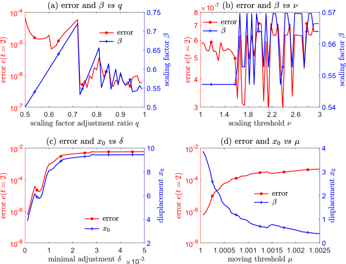
Figure 2: Plots of the error at $t=2$ and the scaling factor $\beta$ or the displacement $x_{0}$ when tuning the scaling factor adjustment ratio $q$ and the scaling threshold $\nu$ or the minimum displacement $\delta$ and the moving threshold $\mu$. (a) The error tends to be smaller as $q$ decreases to $1$, indicating that $q\lesssim 1$ is crucial for proper adjustment of the scaling factor. (b) As $\nu$ is increased, the scaling technique could be impeded, but the error is not very sensitive to $\nu$ if $q$ is small. (c) The error is strongly correlated with $x_{0}$ and a large $\delta$ can lead to over-adjustment of the displacement $x_{0}$, resulting in a larger error. (d) A large $\mu$ will make it harder to activate the moving technique, leading to a smaller $x_{0}$ and a larger error.

Therefore, all three adaptive techniques are expected to be required. Upon setting $\Delta{t}=2\times 10^{-4}$ and solving Eq. (64) up to $t=2$, we investigate how the parameters in the three adaptive techniques affect performance. The initial scaling factor, displacement, and expansion order are set to $\beta=1$, $x_{0}=0$, and $N=40$. First, we test how the scaling threshold $\nu$, the scaling factor adjustment ratio $q$, the moving $\mu$, and the minimum displacement step $\delta$ affect the performance of the scaling and moving techniques. We keep the expansion order fixed since it has been illustrated that the effects of improper scaling or moving can be offset by increasing the expansion order $N$ but at the expense of increased computational cost [3]. Initially, we set the parameters $q=0.99,\nu=1.02,\delta=10^{-4}$, and $\mu=1.00005$, and then change each of them one at a time. Imposing the maximal allowable displacement within each timestep $d_{\max}=0.01$, the upper scaling factor limit $\overline{\beta}=0.2$, and lower scaling factor limit $\overline{\beta}=5$, we plot the relative $L^{2}$-error $e(t=2)$ along with the scaling factor when we change $q$ and $\nu$, and we plot $e(t=2)$ along with $x_{0}$ when we change $\delta$ and $\mu$.

Fig. 2(a) shows that $q\lesssim 1$ is required for the scaling technique to properly adjust the scaling factor. When $q\lesssim 1$ and we vary $\nu$ from $1$ to $2$, the error, as well as the scaling factor $\beta$, do not change much, indicating that the scaling technique is more sensitive to $q$ than to $\nu$. Therefore, keeping $q\lesssim 1$ is more important than keeping $1\lesssim\nu$. Fig. 2(c) shows that the error is highly correlated with $x_{0}$, suggesting that it is critical to properly move the basis functions to capture the displacement of the solution. Having $0\lesssim\delta$ is important so that the displacement $x_{0}$ is not over-adjusted. Finally, as shown in Fig. 2(d), increasing $\mu$ will make the moving technique less sensitive to the translation of the basis functions and lead to a larger error. Thus, $1\lesssim\mu$ is recommended for the moving technique.

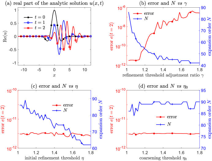
Figure 3: Plots of the real part of the analytic solution $\text{Re}(u)(x,t)$ at different times, the error and the expansion order $N$ at $t=2$ when we vary the refinement threshold adjustment ratio $\gamma$, the initial refinement threshold $\eta$, and the coarsening threshold $\eta_{0}$. (a) The real part of the analytic solution, which translates rightward, becomes more diffusive, and is increasingly oscillatory over time. (b) The error increases with $\gamma$ while the expansion order decreases with $\gamma$. A larger $\gamma$ implies a faster-increasing refinement threshold $\eta$. (c) A larger initial refinement threshold $\eta$ results in a smaller expansion order at $t=2$, yet the error is not reduced as $\eta$ decreases and $N$ increases with the initial $\gamma$. This indicates that as long as $\gamma$ is small enough, a larger initial $\eta$ can be tolerated to lead to a smaller computational cost without compromising accuracy. (d) The expansion order $N$ tends to increase as the coarsening threshold $\eta_{0}$ increases.

Next, we investigate how the initial refinement threshold $\eta$, the refinement threshold adjustment ratio $\gamma$, and the coarsening threshold $\eta_{0}$ affect the $p$-adaptive technique’s performance when $q=0.99,\nu=1.02,\delta=10^{-4}$, and $\mu=1.00005$ are fixed, and the initial variables are set to $\beta=1,x_{0}=0,N=40$. Fixing the maximum increment to $N_{\max}=6$, we start with the initial parameter values $\gamma=1.02$, $\eta=1.05$, and $\eta_{0}=1.02$, and vary each of them one by one and plot the relative $L^{2}$-error and $N$. Fig. 3(a) shows that apart from translating rightward and decaying more slowly, the analytic solution is increasingly oscillatory which requires adjusting the expansion order $N$ of the numerical solution. Fig. 3(b) shows that if $\gamma$ is large, then the threshold for increasing the expansion order $\eta$ will increase more quickly. This renders the $p$-adaptive technique unable to sufficiently adjust the expansion order, leading to smaller expansion orders $N$ and larger errors. Fig. 3(c) shows that the larger the initial threshold $\eta$ for increasing the expansion order, the smaller the expansion order. In the depicted regime, larger initial values of $\eta$ do not degrade accuracy since $N\gtrsim 65$ is sufficient to maintain high accuracy. Therefore, to maintain accuracy while reducing the computational burden, it is crucial to set $1\lesssim\gamma$ so that the $p$-adaptive technique can capture oscillatory behavior over long periods of time. Using a smaller initial $\eta$ may lead to more computational costs but does not lead to improvement in accuracy. Overall, since the function exhibits higher frequency spatial oscillations as time increases, coarsening is typically not activated. However, a large coarsening threshold $\eta_{0}$ can still impede coarsening, resulting in a slightly larger $N$ than a smaller $\eta_{0}$ (Fig. 3(d)).

Finally, as shown in Figs. 2 and 3, we numerically verify that the appropriate strategy for the adaptive spectral parameters is to set $q\lesssim 1,1\lesssim\nu,0\lesssim\delta$, and $1\lesssim\mu$. In fact, for good performance, the scaling procedure strongly requires $q\lesssim 1$ and the moving procedure requires both $0\lesssim\delta$ and $1\lesssim\mu$. For an effective refinement, it is more important to set $1\lesssim\gamma$ rather than to set the initial $1\lesssim\eta$ (i.e., setting $1\lesssim\gamma$ rather than setting the initial $1\lesssim\eta$ leads to more accurate results with smaller computational costs).

Figure 4: Distribution of the collocation points of generalized Hermite functions $\{\hat{\mathcal{H}}_{i,x_{0}}^{\beta}\}_{i=0}^{N}$ with $\beta=1,x_{0}=0$, and $N=24$. $x_{L}\coloneqq x_{[\frac{N}{3}]}^{\beta}$ and $x_{R}\coloneqq x_{[\frac{2N+2}{3}]}^{\beta}$ are marked in red. The number of collocation points that are in the right-exterior region $(x_{R},\infty)$ for calculating $\mathcal{E}_{R}$ and in the left-exterior region $(-\infty,x_{L})$ for calculating $\mathcal{E}_{L}$ are both approximately $N/3$.

When using the generalized Hermite functions defined in $\mathbb{R}$, the desired solution might move leftward or rightward, requiring both leftward and rightward displacement of the basis functions. Since only rightward basis function shifts have been previously considered [3, 4], here, we generalize the moving technique to allow for bidirectional adjustment of the displacement $x_{0}$. It has been proposed that controlling an exterior-error indicator leads to small errors in the exterior domain, relative to the total error, resulting in better approximation of the solution in the exterior region. Therefore, bidirectional moving might maintain relatively small errors in both left- and right-exterior regions of $\mathbb{R}$. We first propose a left exterior-error indicator

$$\mathcal{E}_{L}(U_{N,x_{0}}^{\beta})=\frac{\|\partial_{x}U_{N,x_{0}}^{\beta}\cdot\mathbb{I}_{(-\infty,x_{L})}\|}{\|\partial_{x}U_{N,x_{0}}^{\beta}\cdot\mathbb{I}_{(-\infty,+\infty)}\|},$$ (66)

where we use $x_{L}=x_{[\frac{N}{3}]}^{\beta}$ following the often-used $\tfrac{2}{3}$-rule [5, 6]. The left exterior-error indicator (66) can be seen as the upper bound for the ratio of the error in $(-\infty,x_{L})$ to the error across the whole space $\mathbb{R}$, in analogy to the (right) exterior-error indicator $\mathcal{E}(U_{N,x_{0}}^{\beta})$ defined in Eq. (3), which we shall denote below by $\mathcal{E}_{R}(U_{N,x_{0}}^{\beta})$ for clarity. The number of nodes in the left-exterior region $(-\infty,x_{L})$ and in the right-exterior region $(x_{R},\infty)$ are both roughly $\frac{N}{3}$. It was shown in [4] that if the right exterior-error indicator (3) increases, then the ratio of the error in the right exterior region $(x_{R},+\infty)$ to the total error may also increase, suggesting that one should move the basis functions rightward (increase $x_{0}$). In Fig. 4, we show the positions of collocation nodes of generalized Hermite functions $\{\mathcal{H}_{i,x_{0}}^{\beta}\}_{i=0}^{N}$ with $\beta=1,x_{0}=0$, and $N=24$. The endpoints $x_{L}$ and $x_{R}$ are shown in red, showing that the right and left exterior regions, $(x_{R},\infty)$ and $(-\infty,x_{L})$, are near-symmetric. The left exterior-error indicator  (66) also measures the ratio of the error in the left exterior region $(-\infty,x_{L})$ to the total error, and, if it increases, one can consider shifting the basis functions leftward (decrease $x_{0}$). With both left and right exterior-error indicators, we propose the following bidirectional moving scheme.

Algorithm 1 Pseudo-code of the bidirectional exterior-error-dependent moving technique.

1:Initialize $N$, $\Delta t$, $T$, $\beta$, $x_{0}$, $U_{N,x_{0}}^{\beta}(x,0)$, $\mu>1$, $d_{\rm max}>\delta>0$

2:$t\leftarrow 0$

3:$x_{R}\leftarrow x^{\beta}_{[\frac{2N+2}{3}]}$

4:$x_{L}\leftarrow x^{\beta}_{[\frac{N}{3}]}$

5:$\tilde{\mathcal{E}}_{R}\leftarrow\textsc{right\_exterior\_error\_indicator}(U_{N,x_{0}}^{\beta}(x,0))$

6:$\tilde{\mathcal{E}}_{L}\leftarrow\textsc{left\_exterior\_error\_indicator}(U_{N,x_{0}}^{\beta}(x,0))$

7:while $t<T$ do

8:     $U_{N,x_{0}}^{\beta}(x,t+\Delta t)\leftarrow\textsc{evolve}(U_{N,x_{0}}^{\beta}(x,t),\Delta t)$

9:     $\mathcal{E}_{R}\leftarrow\textsc{right\_exterior\_error\_indicator}({U_{N,x_{0}}^{\beta}(x,t+\Delta{t})})$

10:     $\mathcal{E}_{L}\leftarrow\textsc{left\_exterior\_error\_indicator}({U_{N,x_{0}}^{\beta}(x,t+\Delta{t})})$

11:     if $\mathcal{E}_{R}>\mu\tilde{\mathcal{E}}_{R}~{}||~{}\mathcal{E}_{L}>\mu\tilde{\mathcal{E}}_{L}$ then

12:         $d_{R}\leftarrow\textsc{move\_right}(U_{N,x_{0}}^{\beta}(t+\Delta t),\delta,d_{\rm max},\mu e_{0})$

13:         $d_{L}\leftarrow\textsc{move\_left}(U_{N,x_{0}}^{\beta}(t+\Delta t),\delta,d_{\rm max},\mu e_{1})$

14:         $U_{N,x_{0}}^{\beta}(x,t)\leftarrow\pi_{N,x_{0}+d_{R}-d_{L}}^{\beta}U_{N,x_{0}}^{\beta}(x,t+\Delta t)$

15:         $x_{0}\leftarrow x_{0}+d_{R}-d_{L}$

16:         $x_{L}\leftarrow x_{L}+d_{R}-d_{L}$

17:         $x_{R}\leftarrow x_{R}+d_{R}-d_{L}$

18:         $\tilde{\mathcal{E}}_{R}\leftarrow\textsc{right\_exterior\_error\_indicator}({U_{N,x_{0}}^{\beta}(x,t+\Delta{t})})$

19:         $\tilde{\mathcal{E}}_{L}\leftarrow\textsc{left\_exterior\_error\_indicator}({U_{N,x_{0}}^{\beta}(x,t+\Delta{t})})$

20:     end if

21:     $t\leftarrow t+\Delta t$

22:end while

In Alg. 1, the left_exterior_error_indicator subroutine calculates the left exterior-error indicator by Eq. (66) and the right_exterior_error_indicator calculates the right exterior-error indicator by Eq. (3). If the right or left exterior-error indicator is larger than their corresponding thresholds, i.e, $\mathcal{E}_{R}>\mu\tilde{\mathcal{E}}_{R}$ or $\mathcal{E}_{L}>\mu\tilde{\mathcal{E}}_{L}$, the moving technique is activated, calculating the rightward displacement $d_{0}$ or the leftward displacement $d_{1}$ of the basis functions. In [4], the rightward displacement $d_{R}=\min\{n_{R}\delta,d_{\rm max}\}$ is determined by the move_right subroutine in Line 12, where $n$ is the smallest integer satisfying $\mathcal{E}_{R}(U_{N,x_{0}}^{(\alpha,\beta)}(x-n_{R}\delta,t))<\mu\tilde{\mathcal{E}}_{R}$. Similarly, the leftward displacement $d_{L}=\min\{n_{L}\delta,d_{\rm max}\}$ is determined by the move_left subroutine in Line 13, where $n_{L}$ is the smallest integer satisfying $\mathcal{E}_{L}(U_{N,x_{0}}^{(\alpha,\beta)}(x+n_{L}\delta,t))<\mu\tilde{\mathcal{E}}_{L}$. Notice that the error estimate of the adaptive spectral method in Theorem 1 does not depend on the direction of displacements. Therefore it applies to both the bidirectional moving technique Alg. 1 and the one-sided moving technique proposed in [3].

Example 2.

Consider numerically solving the following parabolic equation in the weak form in $\mathbb{R}\times\mathbb{R}^{+}$

$$(u_{t}(x,t),v)+\big{(}u_{x}(x,t),v_{x}(x,t)\big{)}=\big{(}f(x,t),v(x,t)\big{)},\,\,\,\forall v(x)\in H^{1}(\mathbb{R}),\,\,u(x,0)=e^{-x^{2}}\sin x,$$ (67)

where

$$f(x,t)=\left\{\begin{array}[]{ll}\begin{array}[]{l}\bigg{[}\Big{(}3-2(x+vt)\big{(}v+2(x+vt)\big{)}\Big{)}\sin(x+vt)\\ \hskip 45.52458pt+\Big{(}v+4(x+vt)\Big{)}\cos(x+vt)\bigg{]}e^{-(x+vt)^{2}}\end{array}&t\leq 2,\\[22.0pt] \begin{array}[]{l}\bigg{[}\Big{(}3-4\big{(}x+v(4-t)\big{)}^{2}+2v\big{(}x+v(4-t)\big{)}\Big{)}\sin(x-v(t-4))\\ \hskip 34.14322pt+\Big{(}4x+v(15-4t)\Big{)}\cos(x-v(t-4))\bigg{]}e^{-(x-v(t-4))^{2}}\end{array}&t\geq 2.\end{array}\right.$$ (68)

This PDE is solved by

$$u(x,t)=\left\{\begin{array}[]{ll}\displaystyle e^{-(x+vt)^{2}}\sin\left(x+vt\right)&t\leq 2,\\[13.0pt] \displaystyle e^{-(x-vt+4v)^{2}}\sin\left(x-vt+4v\right)&t\geq 2.\end{array}\right.$$ (69)

We set $v=2$ in Eq. (68) so that the center of the solution moves with velocity $-2$ from $x=0$ to $x=-4$ when $t\in[0,2]$, and when $t\in[2,6]$ the center of the solution moves from $x=-4$ to $x=4$ with velocity $+2$. Since the solution displays only convective behavior, we deactivate the scaling and $p$-adaptive procedures and apply only the moving technique. Since the translation switches from leftward to rightward at $t=2$, the moving technique needs to allow for both leftward and rightward displacement of the basis functions. The parameters in the moving technique are set to be $\mu=1.0005,\delta=0.0005$, and the maximal displacement within a timestep $d_{\max}=0.2$. We take the scaling factor, the expansion order, and the initial displacement of the basis function to be $\beta_{0}=1.2,N_{0}=24,x_{0}=0$, respectively, and plot the results obtained with no moving technique, the leftward-only moving technique, the rightward-only moving technique, and the bidirectional moving technique.

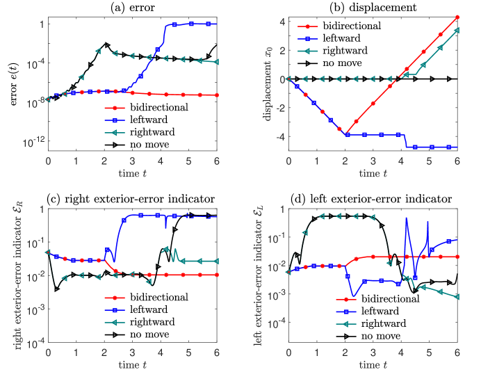
Figure 5: Plots of the error, $x_{0}$, the left exterior-error indicator Eq. (66), and the right exterior-error indicator Eq. (3). (a) The bidirectional moving technique Alg. 1 can main the smallest error while failure to accommodate either leftward or rightward displacement leads to much larger errors. (b,c,d) The displacement $x_{0}$, the left exterior-error indicator, and the right exterior-error indicator of spectral methods with the bidirectional, the leftward-only, the rightward-only moving technique, and the spectral method without any moving.

Fig. 5(a) shows that the spectral method equipped with the bidirectional moving technique (red) can maintain the smallest error because the displacement $x_{0}$ can be decreased when $t\in[0,2]$ and increased when $t>2$ (see Fig. 5(b)). The spectral method with the leftward-only moving technique (blue) can maintain a small error in $[0,2]$ when the center of the function moves leftward but fails to keep the error small when $t>2$ due to its inability to increase $x_{0}$. When $t<2$, the rightward-only moving technique (green) cannot decrease the displacement $x_{0}$ and therefore the error for the rightward-only moving technique is large at $t=2$. Furthermore, large error accumulation before $t=4$ of the rightward-only moving technique makes it unable to properly increase $x_{0}$ for $t>4$ when the center of the solution moves to the right of the origin $x=0$. The right and left exterior-error indicators for the bidirectional moving technique Alg. 1 can be well controlled as shown in Fig. 5(c,d), while for the leftward-only moving technique the right exterior-error indicator grows dramatically when $t>2$ and for the rightward-only moving technique, the left exterior-error indicator grows when $t<2$. Therefore, the leftward- and rightward-only moving techniques both fail to maintain a small error in at least one exterior region $(x_{R},\infty)$ or $(-\infty,x_{L})$. The left exterior-error indicator grows when $t<2$ (the center moves to the left of the origin) and the right exterior-error indicator grows when $t>4$ (the center moves to the right of the origin) for the spectral method without the moving technique (black), suggesting that it cannot maintain a small error in both exterior regions.

5 Discussion and Conclusions

In this paper, we carried out a numerical analysis of recently proposed adaptive spectral methods in unbounded domains using generalized Hermite functions. Specifically, our analysis helps guide parameter choice across three adaptive spectral techniques, i.e., the scaling procedure, the moving procedure, and the $p$-adaptive technique to properly adjust the three key variables associated with these techniques, the scaling factor, the displacement, and the spectral expansion order. Based on our analyses, rules for properly choosing parameters in the scaling, moving, and $p$-adaptive techniques to most efficiently and accurately solve PDEs are derived. We also explicitly explain why controlling the frequency indicator by using adaptive spectral methods effectively controls the error. Numerical experiments were carried out to verify our theoretical results. Furthermore, we developed a new bidirectional moving technique to accommodate both leftward and rightward displacements.

Even though our analysis focused on a simple parabolic model, it nonetheless represents a first step towards understanding how adaptive spectral methods work in solving unbounded-domain problems. In fact, for our parabolic model, the total upper error bound is simply the sum of the errors from numerical discretization and from implementation of the adaptive schemes, providing a clear overall picture of errors under our adaptive spectral algorithm. Additionally, the lower error estimate Eq. (60) holds regardless of the underlying model and numerical discretization, suggesting that controlling a small frequency indicator always leads to a small lower error bound when applying adaptive spectral methods to any model.

Since adaptive spectral methods have been successfully applied to nonlinear PDEs or models containing nonlocal terms [3, 4], further analysis to explain why adaptive spectral methods work well in these more complicated models, particularly in unbounded domains, will be the subject of future investigation. Understanding how adaptive spectral methods work in complex unbounded-domain problems that arise across many disciplines and that are computationally challenging will pave the way for their accurate solution.

Finally, one should also perform analyses of adaptive spectral techniques using other classes of basis functions of recent interest [13]. These include generalized Laguerre functions in $\mathbb{R}^{+}$ and the modified mapped Gegenbauer functions in $\mathbb{R}$. Another potentially useful extension is to explore developing methods to automatically determine and adjust the decay rate of solutions at infinity by adaptively switching among different classes of basis functions in order to match underlying physics or observations.

Funding

TC and MX were supported from the US National Science Foundation through grant DMS-1814364. SS was supported by the National Key R&D program of China (No. 2020AAA0105200) and Beijing Academy of Artificial Intelligence (BAAI).

References

• Ma et al. [2005] Ma, H. and Sun, W. and Tang, T. Hermite Spectral Methods with a Time-Dependent Scaling for Parabolic Equations in Unbounded Domains. SIAM J. Numer. Anal., 43:58–75, 2005.
• Shen et al. [2011] Shen, J. and Tang, T. and Wang, L. L. Spectral Methods: Algorithms, Analysis and Applications. Springer Science & Business Media, 2011.
• Xia et al. [2021] Xia, M. and Shao, S. and Chou, T. Efficient scaling and moving techniques for spectral methods in unbounded domains. SIAM J. Sci. Comput., 43(5):A3244–A3268, 2021.
• Xia et al. [2021] Xia, M. and Shao, S. and Chou, T. A frequency-dependent p-adaptive technique for spectral methods. J. Comput. Phys., 446:110627 , 2021.
• Hou & Li [2007] Hou, T. Y. and Li, R. Computing nearly singular solutions using pseudo-spectral methods. J. Comput. Phys., 226:379–397, 2007.
• Orszag [1971] Orszag, S.A. On the Elimination of Aliasing in Finite-Difference Schemes by Filtering High-Wavenumber Components. J. Atmos. Sci, 28:1074–1074, 1971.
• Moler & Van Loan [1978] Moler, C. and Van Loan, C. Nineteen dubious ways to compute the exponential of a matrix, twenty-five years later. SIAM Rev., 20(4):801–836, 1978.
• Babuska et al. [2012] Babuska, I. and Flaherty, J.E. and Henshaw, W.D. and Hopcroft, J.E. and Oliger, J.E. and Tezduyar, T.eds. Modeling, mesh generation, and adaptive numerical methods for partial differential equations. Springer Science & Business Media, 2012.
• Tang & Tang [2020] Tang, H. and Tang, T. Adaptive mesh methods for one-and two-dimensional hyperbolic conservation laws. SIAM J. Appl. Math., 80(3):1307—1335, 2020.
• Ren & Wang [2000] Ren, W. and Wang, X.P. An iterative grid redistribution method for singular problems in multiple dimensions. J. Comput. Phys., 159(2):246–273, 2000.
• Li et al. [2002] Li, R. and Liu, W. and Ma, H. and Tang, T. Adaptive finite element approximation for distributed elliptic optimal control problems. SIAM J. Control Optim., 41(5):1321–1349, 2002.
• Xia et al. [2020] Xia, M. and Greenman, C.D. and Chou, T. PDE models of adder mechanisms in cellular proliferation. SIAM J. Appl. Math., 80(3):1307–1445, 2020.
• Tang et al. [2020] Tang, T. and Wang, L.L. and Yuan, H. and Zhou, T. Rational spectral methods for PDEs involving fractional Laplacian in unbounded domains. SIAM J. Sci. Comput., 42(2):A585–A611, 2020.
• Li et al. [2018] Li, B. and Zhang, J. and Zheng, C. Stability and error analysis for a second-order fast approximation of the one-dimensional Schrödinger equation under absorbing boundary conditions. SIAM J. Sci. Comput., 40(6):A4083–A4104, 2018.
• Xia & Chou [2021] Xia, M. and Chou, T. Kinetic theory for structured populations: application to stochastic sizer-timer models of cell proliferation. J. Phys. A-Math. Theor., 54(38):385601, 2021.
• Hügli et al. [2012] Hügli, R.V. and Duff, G. and O’Conchuir, B. and Mengotti, E. and Rodriguez, A.F. and Nolting, F. and Heyderman, L.J. and Braun, H.B. Artificial Kagome spin ice: dimensional reduction, avalanche control and emergent magnetic monopoles. Philos. T. R. Soc. A, 370(1981):5767–5782, 2012.
• Mengotti et al. [2012] Mengotti, E. and Heyderman, L.J. and Rodriguez, A.F. and Nolting, F. and Hügli, R.V. and Braun, H.B. Real-space observation of emergent magnetic monopoles and associated Dirac strings in artificial Kagome spin ice. Nat. Phys., 7(1):68–74, 2011.
• Xiong & Guo [2022] Xiong, Y. and Guo, X. A short-memory operator splitting scheme for constant-Q viscoelastic wave equation. J. Comput. Phys., 449:110796, 2022.
• Ueda & Saito [2019] Ueda, Y. and Saito, N. The inf-sup condition and error estimates of the Nitsche method for evolutionary diffusion–advection-reaction equations. Jpn. J. Ind. Appl. Math., 36(1):209–238, 2019.
• Dautray & Lions [1992] Dautray, R. and Lions, J.L. Mathematical analysis and numerical methods for science and technology: volume 5 evolution problems I. Springer, 1992.
• Lin et al. [2014] Lin, Q., Luo, F., and Xie, H. A posterior error estimator and lower bound of a nonconforming finite element method. J. Comput. Appl. Math., 265: 243-254, 2014.
• Tang [1993] Tang, T. The Hermite spectral method for Gaussian-type functions. SIAM J. Sci. Comput., 14(3):594–606, 1993.
• Antonietti et al. [2019] Antonietti, P. and Canuto, C. and Verani, M. An Adaptive hp–DG–FE Method for Elliptic Problems: Convergence and Optimality in the 1D Case. Commun. Appl. Math. Comput., 1(3):309–331, 2019.
• Xiang & Wang [2010] Xiang, X.M. and Wang, Z.Q. Generalized Hermite spectral method and its applications to problems in unbounded domains. SIAM J. Numer. Anal., 48(4):1231–1253, 2010.
• Tang & Xu [2007] Tang, T. and Xu, J.C. Adaptive Computations: Theory and Algorithms. Science Press, Beijing, 2007.