Galaxy And Mass Assembly (GAMA): Self-Organizing Map Application on Nearby Galaxies

Abstract

Galaxy populations show bimodality in a variety of properties: stellar mass, colour, specific star-formation rate, size, and Sérsic index. These parameters are our feature space. We use an existing sample of 7556 galaxies from the Galaxy and Mass Assembly (GAMA) survey, represented using five features and the K-means clustering technique, showed that the bimodalities are the manifestation of a more complex population structure, represented by between 2 and 6 clusters. Here we use Self Organizing Maps (SOM), an unsupervised learning technique which can be used to visualize similarity in a higher dimensional space using a 2D representation, to map these five-dimensional clusters in the feature space onto two-dimensional projections. To further analyze these clusters, using the SOM information, we agree with previous results that the sub-populations found in the feature space can be reasonably mapped onto three or five clusters. We explore where the “green valley" galaxies are mapped onto the SOM, indicating multiple interstitial populations within the green valley population. Finally, we use the projection of the SOM to verify whether morphological information provided by GalaxyZoo users, for example, if features are visible, can be mapped onto the SOM-generated map. Voting on whether galaxies are smooth, likely ellipticals, or “featured" can reasonably be separated but smaller morphological features (bar, spiral arms) can not. SOMs promise to be a useful tool to map and identify instructive sub-populations in multidimensional galaxy survey feature space, provided they are large enough.

1 Introduction

Quantitative galaxy classification has relied on luminosity, colour, the type of Sérsic profile (Sérsic, 1968) or colour and mass segregation. In such classifications, bimodalities were very often identified in the local Universe (cf. Graham, 2019). In colour space, there are two distinct populations; one with blue optical colours and another with red optical colours and higher stellar masses (Baldry et al., 2006; Willmer et al., 2006; Ball et al., 2008; Brammer et al., 2009). These populations were dubbed the “blue cloud” and the “red sequence” respectively (Driver et al., 2006; Faber et al., 2007; Taylor et al., 2015). This can be translated into a bimodality of specific star-formation (i.e. relative growth of the galaxy) with a “star-forming galaxy sequence" and a “quiescent" population (Noeske et al., 2007; Wang et al., 2016).

Similarly, disk and spheroidal galaxies show a bimodal distribution in their Sérsic (Sérsic, 1963) profiles (Vulcani et al., 2014; Kennedy et al., 2015, 2016a, 2016b; Moffett et al., 2016a, b, Casura in prep.), moving from pure disk (Sérsic index n=1) to pure spheroidal (Sérsic index n=4). By and large, much of the bimodalities seem to correspond to two populations: disk-dominated, star-forming blue galaxies and spheroidal, “red and dead" quiescent ones. This bimodality is clearest for stellar masses over $10^{10}~{}M_{\odot}$, while at lower stellar masses the bimodality disappears (Graham et al., 2006).

Turner et al. (2019) explored K-means clustering in the multi-dimensional parameter space of nearby galaxies observed with the Galaxy And Mass Assembly (GAMA, Driver et al., 2009) survey. The high completeness of the spectroscopic redshift component of the GAMA survey combined with multi-wavelength coverage ensured that this is a highly complete census of galaxy populations in the nearby Universe.

Turner et al. (2019) found that the bimodalities observed in mass or colour did not translate into direct correspondence with morphological features, i.e. not all disk galaxies are blue and star-forming, something already noted by Masters et al. (2010) using GalaxyZoo. How many actual clusters of galaxy populations there are remained unclear from the K-means clustering in Turner et al. (2019). More than two and up to six plausible clusters could be identified in the GAMA data using K-means clustering.

Similarly, the notion that the “green valley" of galaxies in mass-colour space was a single transitioning population has been questioned using galaxy morphology (Schawinski et al., 2014; Salim, 2015) but it does have more prevalent morphological features (Bremer et al., 2018; Kelvin et al., 2018) and subpopulations show evidence of quenching (Smethurst et al., 2015, 2017; Belfiore et al., 2017; Phillipps et al., 2019; Bluck et al., 2020), though not driven primarily by major mergers (Weigel et al., 2017).

There is some evidence that certain morphological subgroups are more common in the green valley (Bremer et al., 2018; Kelvin et al., 2018, Smith in prep), and that major mergers are not very prevalent in the green valley (Weigel et al., 2017). However, a sizable sub-population is quenching (Smethurst et al., 2015, 2017; Rowlands et al., 2018; Belfiore et al., 2017; Phillipps et al., 2019) and certain morphological features may become more visible as a result, especially given that the quenching appears to be happening inside-out and not galaxy-wide (Bluck et al., 2020).

In this paper, we explore a different unsupervised learning algorithm on the same data-set to visualize the possible sub-populations of galaxies. Unsupervised machine learning to explore galaxy morphology is becoming quite common (e.g. Cheng et al., 2021; Turner et al., 2021). We use the Self Organizing Maps (Kohonen, 2001) to reduce the dimensionality of the feature data set to a single two-dimensional map. SOM has been used on galaxy morphology and colours before (e.g., Naim et al., 1997; Hemmati et al., 2019; Davidzon et al., 2019) but the new GAMA feature space opens many new possibilities for application of SOM for galaxy morphology and other properties.

Our goals are to verify the population clustering underlying the multiple subpopulations that are revealed by the K-means study in Turner et al. (2019), to explore the intermediate population of one bimodality (the green valley population), and evaluate how GalaxyZoo classifications are mapped onto this SOM. By mapping the K-means clustering classifications onto a SOM, we will explore how many separate clusters of galaxy populations can be identified in the GAMA data. Secondly, we will see how the colour bimodality is mapped onto the SOM to identify and map the interstitial green valley population. Lastly, we will map the voting records of the GalaxyZoo project onto the SOM as an alternate label to evaluate how well galaxy-wide feature space can map detailed visual morphology. Section 2 briefly describes our subsample of the full GAMA catalogs. Section 3 describes the K-means result and section 4 describes the details of SOM training. Section 5 goes through how the K-means cluster (§5.1), green valley (§5.2), and GalaxyZoo votes (§5.3) are mapped onto the SOM. Section 6 contains our concluding remarks.

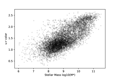
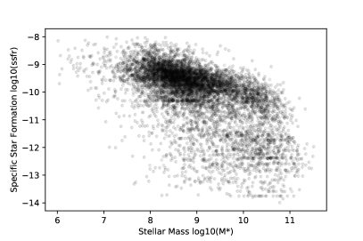
Figure 1: The four features (u-r colour, specific star-formation rate, Sérsic index $n$, and half-light radius, $r_{50}$) as a function of stellar mass for the GAMA subsample of Turner et al. (2019). Each distribution shows the bimodality often with one strong locus and one less pronounced.

2 GAMA Subset

We will use the exact same input dataset derived from the GAMA equatorial catalogs as did Turner et al. (2019) for their K-means clustering analysis.

Briefly, they used redshift and mass limited samples from phase II of the Galaxy And Mass Assembly (GAMA) survey (Driver et al., 2009; Liske et al., 2015). The main aim of the survey is to study cosmic structure on scales ranging from 1 kpc to 1 Mpc, focusing on groups and their environments. The survey is centered around the spectroscopic campaign, conducted with the Anglo-Australian Telescope using the AAOmega spectrograph (target catalog in Baldry et al., 2010). Reliable redshifts are available for 238000 objects to a limiting r-band magnitude of 19.8 and across five regions covering a total area of 286 deg².

The spectroscopic component of GAMA has been supplemented with reprocessed imaging in 21 bands from a variety of other surveys (e.g. the Sloan Digital Sky Survey; York et al., 2000) and the Kilo-Degree Survey (KiDS de Jong et al., 2013; de Jong et al., 2015, 2017; Kuijken et al., 2019) that overlap with the GAMA spectroscopic campaign footprint (the Panchromatic Data Release Driver et al., 2016). Value-added data derived from these spectra and images are listed in tables hosted at http://www.gama-survey.org.

Turner et al. (2019) modeled their sample after that of Moffett et al. (2016a): this is a low-redshift ($0.002<z<0.06$) and magnitude-limited ($r_{PETRO}<19.8$) sample of 7556 local objects that have been morphologically classified using the method of Kelvin et al. (2014).

In addition to the Kelvin et al. (2014) morphological classification, there are now Galaxy Zoo classifications (Lintott et al., 2008, Kelvin et al., in prep.) with votes on disk or spheroid, prominence of bulges, shape of bulges, number and winding of spiral arms, and rarer morphology such as mergers (cf Holwerda et al., 2019, for dust lanes in this GalaxyZoo data).

The Turner et al. (2019) sample’s feature space consisted of stellar mass ($M_{*}$), $u-r$ colour, specific star-formation rate (ssfr), Sérsic index ($n$) and half-light ($r_{50}$). The stellar masses ($M_{*}$) and the specific star formation (ssfr) on a Gyr timescale are from the MAGPYS (da Cunha et al., 2008) 21-filter SED fit catalog (MagPhysv06) described in Driver et al. (2016). The input for this SED fit is the LambdarCatv01 (Wright et al., 2016). The restframe $u-r$ colour is based on this LAMBDAR photometry, corrected for redshift (StellarMassesLambdarv20), using the same formalism as Taylor et al. (2011), but not corrected for dust effects. The r-band Sérsic indices (n) and half-light radii ($r_{50}$) are from the analysis of Sloan Digital Sky Survey images described in Kelvin et al. (2012), SersicCatSDSSv09 in GAMA repository. These catalogs are readily available at http://www.gama-survey.org/dr3/.

Our feature selection is entirely based on the one from Turner et al. (2019) because it is in this space is where the bimodalities occur. The feature space is a mixture of observed (e.g. restframe $u-r$ colour) and derived parameters (e.g. specific star-formation rate). The derived values may have systematic effects in their values (e.g. mass-to-light ratio for stellar masses). However, the feature space is whitened (scaled to standard deviation and mean set to 0) and should suffice for relative discrimination. These are the features on which the K-means clustering was based and we will train our Self Organizing Map on.

We should note here that the feature sample is not evenly balanced between bimodalities. Figure 1 shows the distributions of the features used in the K-means clustering. Each panel shows signs of the bimodalities noted earlier but like most real data, the clusters are not neatly separated and not with equal representation in the data.

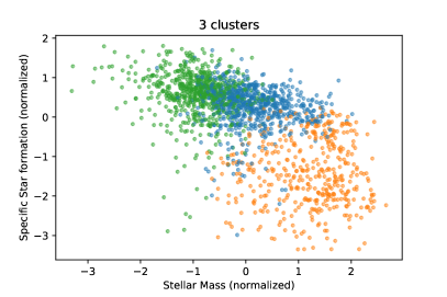
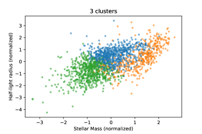
Figure 2: The four features (u-r colour, specific star-formation, Sérsic index n and half-light radius $r_{50}$) as a function of stellar mass, now all normalized and whitened for use by the K-means clustering algorithm. The 3 K-means clusters from Turner et al. (2019) identified are indicated in the normalized feature space.

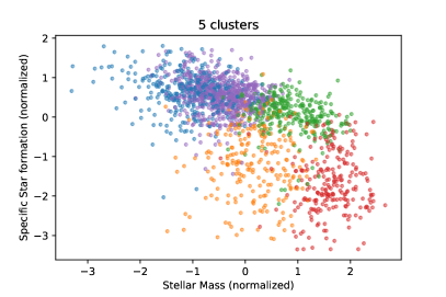
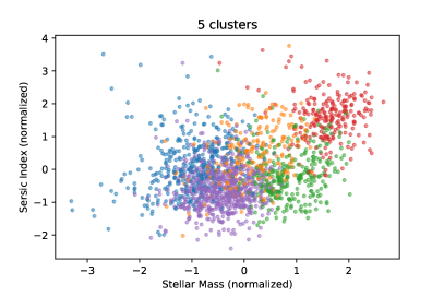
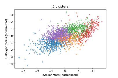
Figure 3: Same as Figure 2 but now for the 5 cluster space indicated with colours.

3 K-means Clustering

Although K-means worked well on this data-set, it is important to reiterate that a drawback of K-means method is that we have to specify the number of clusters, $k$, as an input. The optimal value of $k$ is generally not known in advance, hence the optimal value must be identified by clustering at several different values of $k$ and analysing the outcomes afterwards. The number of clusters to choose is not necessarily obvious in real-world applications such as these, especially in the case of a higher dimensional data-set or one that is not distributed equally among the number of clusters. This is an issue Turner et al. (2019) encountered and noted as well. Figures 2 and 3 illustrate the clustering in the whitened feature space. Both a 3-cluster or 5-cluster solution is just as visually appropriate.

We will now first examine the optimal number of clusters in this sample, using the K-means clustering implementation in scikit-learn. In Turner et al. (2019), the optimal number of clusters was addressed by examining the stability of clustering outcomes over large numbers of randomised initialisations. The elbow method is a useful graphical tool to estimate the optimal number of clusters $k$. If $k$ increases, the within-cluster Sum of Squared Errors (SSE, or “inertia” or “distortion”) should decrease, because the samples will be closer to the centroids they are assigned to.

The idea behind the elbow method is to identify the value of $k$ where the distortion decreases most rapidly. This is shown in Figure 4 which plots the SSE as a function of number of clusters $k$ for the GAMA data-set.

We conclude from this plot that the optimal number of clusters is between 2 and 5 with which to classify the GAMA data-set, in agreement with Turner et al. (2019). Three clusters appear optimal, showing that the bimodalities noted in this feature space is not a single underlying bimodality but are comprised of subpopulations.

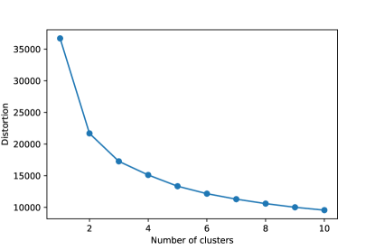
Figure 4: The distortion (also known as inertia or SSE) as a function of the number of clusters employed on the normalized GAMA sample. The conclusion that the optimal number lies somewhere between k=2 and k=5.

$N_{clusters}$	$S_{train}$	$S_{test}$
2	0.395	0.407
3	0.260	0.266
4	0.231	0.239
5	0.238	0.245
6	0.230	0.228

Table 1: The Silhouette coefficients for the K-means classifications for each of the numbers of clusters. Values that are significantly lower than 1, like those observed here, indicate significant overlapping among clusters.

To evaluate the K-means clustering here further, we employ the silhouette coefficient (sklearn.metrics). The values for the training and test sample for each number of clusters are listed in Table 1. The silhouette coefficient is calculated from the mean intra-cluster distance (a) and the mean distance to the nearest-cluster to which the sample does not belong (b):

$$S=\langle(b-a)/max(a,b)\rangle.$$ (1)

over the whole sample. Optimal coefficient value is 1 and the poorest clustering is denoted by -1 (misclassification). Values near 0 indicate overlapping clusters. In an optimal application scheme, clusters are well separated, i.e. $b>>a$ and $max(a,b)=b$, so the silhouette coefficient is close to 1. Lower values indicate overlapping clusters.

The values in Table 1 show values closer to 0 than 1, indicating that the clusters are not well-separated (as can be seen in Figures 2 and 3). K-means clustering is ideal for isomorphic (rounded) and balanced clusters (approximately equal numbers of objects in each cluster). This may not necessarily be the case here (Figure 1). We checked with scikit-learn’s Density-Based Spatial Clustering of Applications with Noise (DBSCAN) as an alternate clustering algorithm as well but this performed poorly in comparison (lower or even negative silhouette coefficients). We conclude that in this feature space, there is significant overlap among clusters.

Self Organizing Maps can be used to generate a 2-dimensional map of a higher-dimensional feature space; vicinity in the SOM space is associated with similarity in the original feature space. This is not the only alternative, for example, one could employ a Principal Component Analysis (PCA Conselice, 2006; Scarlata et al., 2007) or alternate clustering algorithms (Turner et al., 2021). We opt for SOM for the ease of visualization. Another advantage is that SOMs are non-linear, which helps to preserve both global and local structures from the high-dimensional feature space in the final projection.

4 Self Organizing Maps

Using the full 7556 sources in the GAMA nearby galaxy sample, we train a $100\times 100$ size SOM for 1000 iterations using the minisom (Vettigli, 2019) Python implementation of Self-Organizing Maps. Input data is the set of features, a vector for each object of Stellar mass, specific star-formation rate, u-r colour, Sérsic index, and effective radius, all renormalized (also known as “whitened”) to ensure a mean of 0 and scaling to their standard deviation.

Self Organizing Maps are an early form of unsupervised learning (cf. Kohonen, 2001). Briefly, a map is seeded with random vector nodes that resemble the (whitened) data in mean and standard deviation. During training, a data point is picked at random, and its closest node in the SOM, known as Best Matching Unit or BMU, is found, and the coordinates of the BMU and its surrounding nodes are updated to move towards that data point. At each learning iteration, the full data-set is applied to the SOM, modifying its “winning” nodes and neighbors to resemble the data instance more. The process is repeated for many iterations; once converged, the final network of nodes of the SOM should be topologically close to the full data set. A SOM is ideal if no clear number of classes is known beforehand and one wants to map a multi-dimensional feature space onto a single two-dimensional map.

Because the initialization of the SOM is a randomized event, the learning process for each time the SOM is trained will result in a different SOM. The only hyperparameter for the SOM is its size, which determines its resolving power, and the choice of learning function, which optimizes how long it takes to converge.

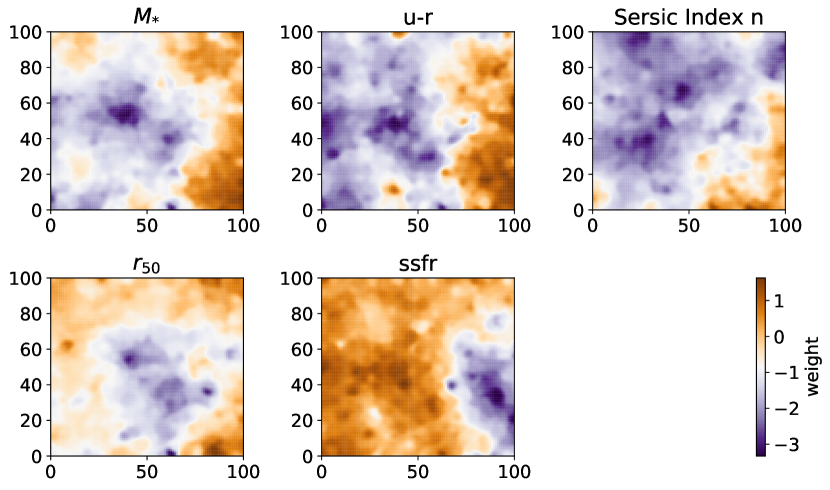
Figure 5: The five features (u-r colour, specific star-formation, Sérsic index n, half-light radius $r_{50}$ and stellar mass) mapped from the multidimensional parameter space onto our SOM to show their relative weight in each SOM node on the map.

The SOM we have generated provides a 2-D representation of our sample where similarity is preserved: objects that are close in the higher-dimensional feature space should be close also in the SOM. Therefore, we can use the SOM as a “canvas” onto which we map other properties, such as individual features, or the clustering structure identified by the k-means algorithm, to understand how these relate to the higher-dimensional representation of our sample. Figure 5 shows where the feature space is mapped onto this instance of the SOM. Because a SOM is initiated with a random seed, the map would appear different after each initiation and training. For a SOM different initialisations would still be expected to yield the same results at a qualitative level (i.e. clusters would still appear grouped together, even if they show up somewhere else in the map). We retrained this SOM several times each time arriving at the same qualitative result.

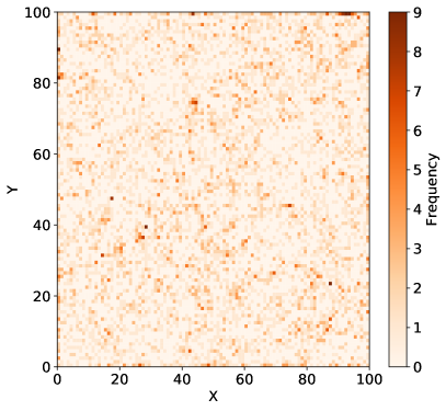
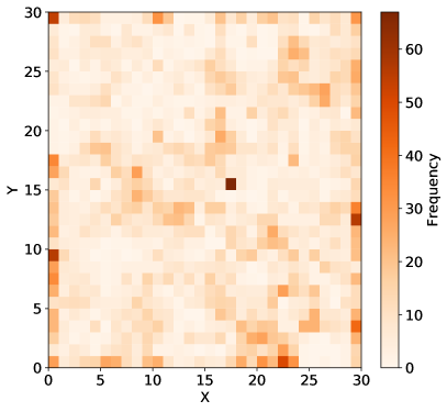
Figure 6: The frequency map of our SOM: the frequency each node is the winning one in classifying the sample. The $100\times 100$ (left) and a $30\times 30$ (right). The scale of the SOM is the predominant hyper-parameter for SOM. In a lower resolution version, a few nodes attract high numbers of sources, losing resolution in those areas while SOM in-between these remains much lower populated.

Specific star-formation and $u-r$ colour are most closely related in the weighting of the SOM. This is consistent over multiple training runs of the SOM. This should not surprise us as u-r is a star-formation tracer. It serves to remind us that the feature space is not orthogonal but somewhat degenerate.

Figure 6 shows the winning frequency of each node when classifying the full sample. Maximum frequency is 9. The overall size of the SOM and resulting total number of nodes may be somewhat generous for the size of this sample. Figure 6 compares the frequency of matches between our data and a SOM node for the 100$\times$100 SOM and a 30$\times$30 one trained on the same data-set. The smaller SOM trains faster but corrals objects in a few nodes, leaving less resolution to differentiate sub-populations.

To evaluate the quality of a feature map, we use two indicators: learning quality and projection quality. Quantization error and topographical error are our main measurements to assess the quality of SOM. Quantization error is the average difference of the input samples ($x(t)$) compared to its corresponding winning map point ($w(t)$). It assesses the accuracy of the represented data, therefore, it is better when the value is smaller.

$$QE={1\over T}\Sigma_{t=1}^{T}||x(t)-w(t)||$$ (2)

where $x(t)$ is the input sample at the training t; $w(t)$ is the BMU’s weight vector of sample $x(t)$; $T$ is total of training iterations.

The topographical error indicates the number of the data samples having the first best matching SOM node (SOM-1) and the second best matching SOM node (SOM-2) being not adjacent, i.e. how well is the sample segregated and grouped together in similarity? In a well assembled SOM, the closest node and the next-to-closest node are expected to be adjacent, and therefore this fraction should be small.

$$TE={1\over T}\Sigma_{t=1}^{T}d(x(t)),$$ (3)

where $x(t)$ is the input sample at training times $t$; $d(x)$ is a step function where, $d(x(t))=1$ if SOM-1 and SOM-2 (the closest and second closest match in the SOM) for $x(t)$ are not adjacent and $d(x(t))=0$ if they are. T is total of all training times. The more often the two best SOM nodes are adjacent, the lower TE will be. Figure 7 shows the two learning curves for 1000 iterations. Both stabilize after 1000 iterations and we adopt (and save) this SOM for further use.

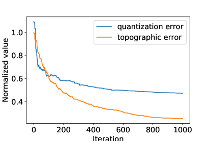
Figure 7: The learning curves of the SOM over 1000 iterations. The Quantization Error (blue) improves first and gain is steady with each iteration. The topographical error (orange) improves a little later (SOM rearranges itself) and then converges.

5 Results

We explore three sets of properties as they are mapped onto the SOM. First the classification by the K-means clustering algorithm. Secondly, the position of green valley galaxies as mapped onto the SOM. And thirdly, we explore how GalaxyZoo voting is distributed over the SOM.

5.1 K-Means Clusters

Our first objective is to evaluate how the different K-means clusters are mapped onto the SOM. Figure 8 shows how each of the clusters from Turner et al. (2019) is distributed onto the SOM. In each of the mappings of the K-means clusters onto the SOM, very few nodes are split between multiple K-means clusters showing that the SOM discriminates well between these in the feature space (the SOM is both big enough and well-trained enough). The feature space has enough resolution to make the separation meaningful for the K-means clusters.

From Figure 8 it appears that K2 or K3 works slightly better on this feature space than K5 of K6. The low degree of mixing between object in different clusters suggests that K2 or K3 clusters provide a better representation of our sample, compared to K5 or K6 clusters. The latter two break into too many sub groupings to improve classification much over K2 or K3.

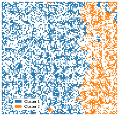
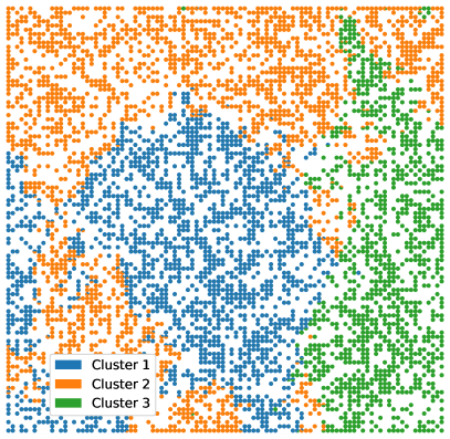
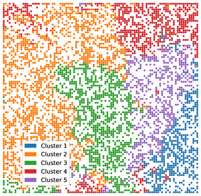
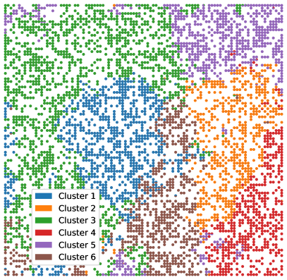
Figure 8: Pie diagrams of each cluster of the $100\times 100$ SOM trained on the GAMA feature set. The pie diagrams show if unique K-means clusters are attributed to each SOM node. The amount of mixing is an index of the quality of the clustering. For the most part, K-means clusters are mapped onto unique SOM nodes with little mixing. The K2 and K3 clustering remain coherent (mostly single continuous areas on the SOM).

5.2 Green Valley Galaxies

A prime example of an intermediate population of galaxies is the “green valley", the galaxies in global colour that sit between the star-forming sequence and the quiescent red cloud. Green valley galaxies’ intermediate colours are commonly interpreted as a population of galaxies transitioning from star-forming to passive.

Bremer et al. (2018) present a working definition based on stellar mass and the restframe, dust corrected $u-r$ colour, also adopted in Kelvin et al. (2018). We start with the adoption of this colour criterion for the green valley but extrapolate the definition to the entire mass range of our sample rather than the narrow mass range used in Bremer et al. (2018). Figure 9 shows the colour cuts in $u-r$ colour –uncorrected for dust– and stellar mass space. The green valley population starts a little above $10^{9}M_{\odot}$ stellar mass and the division at lower mass is just between red and blue galaxies. This is consistent with the picture in Taylor et al. (2011) who model the stellar mass and $u-r$ colours of GAMA galaxies.

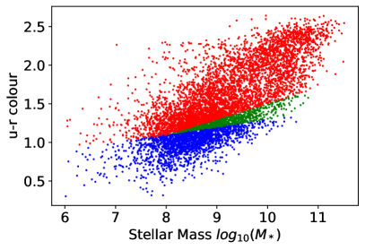
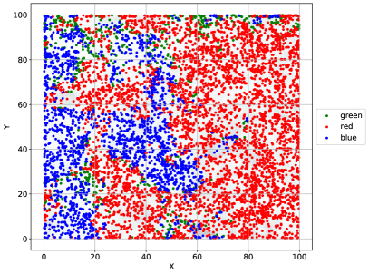
Figure 9: The $u-r$ colour as a function of stellar mass for the GAMA sample of Turner et al. (2019). The green valley criteria from Bremer et al. (2018) are shown for the full mass range. The position of the green valley galaxies identified in Figure 9 on the SOM. Green valley galaxies, a canonical transitional population in one part of this feature space, are found all over the SOM map of the full feature space.

Figure 9 shows where the red and blue galaxies and the green valley galaxies according to the uncorrected Bremer et al. (2018) colour criterion are mapped onto the SOM. Both red and blue galaxies are made up of several clusters on the map and green valley galaxies only concentrate on a few nodes in between the red and blue populations. The blue and red populations are spread over the SOM as blue and red subpopulations end up at different nodes, separated e.g. by stellar mass. The blue and red coherence is driven by the colour and specific star-formation rate, with the substructure and partial fragmentation reflecting the more distinct galaxy red and blue sub-populations.

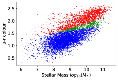
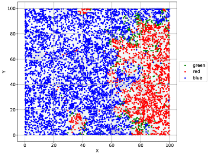
Figure 10: Left: The $u-r$ colour as a function of stellar mass for the GAMA sample of Turner et al. (2019) corrected for extinction ($u-r+0.4$) to bring these in line with Bremer et al. (2018). The green valley criteria from Bremer et al. (2018) are shown for the full mass range. Right: the position of the green valley galaxies identified on the SOM. Green valley galaxies, a canonical transitional population in one part of this feature space, are found all over the SOM map of the full feature space. Compare this colour corrected for dust (as a population, not individually) with the specific star-formation criterion in Figure 11.

Turner et al. (2019) used $u-r$ colours that had not been corrected for internal dust attenuation and this has been our feature space. However, Bremer et al. (2018) use the $u-r$ colours that are dust-corrected. Here, we apply an general offset to the Bremer et al. (2018) green valley definition in order to reflect this difference. Turner et al. (2019) did something similar to divide between red and blue galaxies. Following this, we apply a +0.4 mag shift to the $u-r$ colour criteria from Bremer et al. (2018) in Figure 10 and show where the corrected colours land on the SOM.

If we compare Figure 5 to Figure 10, several sub-populations can be identified. Previously, Schawinski et al. (2014) pointed out that the green valley is no single population of galaxies but a mix of several intermediate groups (see also Smethurst et al., 2015; Moutard et al., 2016).

There are two red/green clumps amidst the blue populations at x=35,y=10 and x=40,y=100 on the SOM visible in Figure 10. These correspond to different colours and high-mass galaxies in Figure 5. Concentrations of green galaxies can be identified around X=80,Y=10 and X=80,Y=90, correspinding to high-mass and extended galaxies with a steep profile ($log(n)\simeq 1$) characteristic of ellipticals or bulge-dominated disk galaxies.

The SOM applications show that in the feature space, the green valley galaxies are not one single intermediate group (i.e. a single group of nodes with just green galaxies) but several small intermediate populations combined. Morphology studies of the green valley have shown that it is made up of both disk galaxies and ellipticals, and the galaxy disks are dimming and perhaps forming rings (Kelvin et al., 2018; Fernandez et al., 2021, Smith et al. in prep.), perhaps driven by bars in secular evolution (e.g, Géron et al., 2021). Morphological features not included in our feature space (e.g. rings and bars) are drivers of this evolution of these sub-populations. The different “interstitial” sub-populations are distinct enough in the galaxy-wide feature space to be separated out in our SOM, but other features may better distinguish them from each other.

The multiple green valley populations sandwiched between red and blue populations on the SOM support the idea that the green valley population of galaxies is “interstitial” rather than exclusively a single transitioning population of galaxies. We note that Bremer et al. (2018) only employed the green valley criterion in a narrow mass range and for corrected $u-r$ colours. If we restrict ourselves to this mass range ($10.25<log_{10}(M^{*})<10.75$), we are predominantly left with red galaxies in our sample.

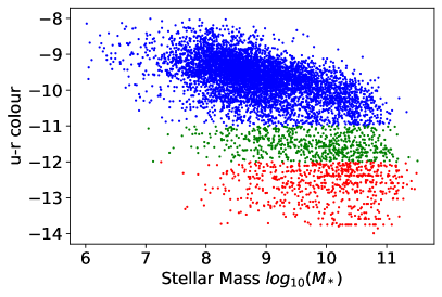
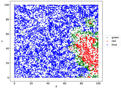
Figure 11: The definition for the green valley using specific star-formation rate from Salim (2015) for our nearby sub-sample from Turner et al. (2019). The position of the green valley galaxies according to the criterion in Salim (2015) based on the specific star-formation ($-12<log_{1}0(SSFR)<-11$). This criterion separates the red from the blue populations with a ring of green objects. A few sub-nodes of red galaxies with green borders can be found as well.

Salim (2015) notes in their overview of green valley galaxy properties that these u-r optical colours may only allow for a poor separation in the level of star-formation. Ultimately, the green valley is defined as an intermediate star-forming population. Figure 11 shows the green valley as defined as specific star-formation levels between $-12<log10(SSFR)<-11$. We note that both the uncorrected $u-r$ colour and the specific star-formation were inputs in the SOM training.

Figure 11 shows the distribution of blue, green, and red galaxies based on the definition in specific star-formation rate in Figure 11. The blue and red populations separate out in two unique groups with the green valley galaxies in between. We note that there are several small “pockets" of red galaxies unique in Sérsic index or stellar mass (see Figure 5).

Both the corrected $u-r$ colour definition and the specific star-formation definition of the green valley mapped onto the SOM point to sub-populations in the green valley based on stellar mass, profile, or both.

The K-means clustering was applied by Turner et al. (2019) to identify the number of bi-modalities in this parameter space. The green valley is in the saddle point of one of these bi-modalities. We shall briefly compare the position of the green valley on our SOM and compare it to the disposition of the K-means clusters.

Using the $u-r$ colour definition, we compare Figure 9 to the earlier mapping of the K-means nodes in Figure 8. The red and blue clouds correspond fairly closely to different K-means nodes; for example, the red cloud corresponds to cluster 3 in the 3-cluster classification with the blue cloud corresponding mostly to cluster 1 and 2. The green valley galaxies are evenly split as either one or the other K-cluster.

The corrected $u-r$ colour selected green valley galaxies reside in more specific nodes in the higher K-means classifications. For example, in the 5-cluster classification, the low-mass green valley galaxies are in cluster 4. And in the K-6 cluster solution, the green valley galaxies correspond largely to outlier sections of one of the K-means clusters (cluster 5). Most of the K-means cluster 5 is still a coherent structure on the SOM but the transitioning or interstitial populations are classified in completely different nodes of the SOM.

Using the specific star-formation definition of the green valley (Figure 11), we observe the same trend. We compare Figure 11 to the K-means clusters in Figure 8, it is clear that red and blue populations are associated with one or two clusters in the K2 or K3 classification. But even in higher order K-means clustering, the green valley galaxies are never grouped in a single K-means cluster and always evenly split between K-nodes.

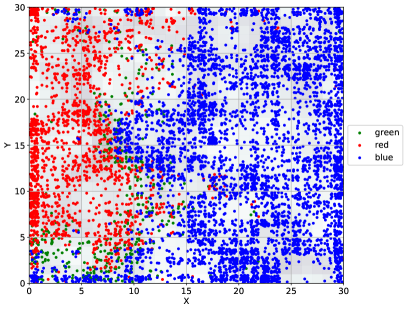
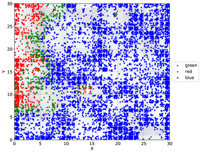
Figure 12: The position of the green valley galaxies identified in the $30\times 30$ SOM (see also Figure 6). Left: the blue, green, and red classification based on corrected $u-r$ colour criteria shown in Figure 10. Right: the blue, green, and red classification based on specific star-formation rate shown in Figure 11.

Part of our motivation for this work was to evaluate how good SOM mapping is to identify smaller galaxy sub-populations in a well-understood sample, previously classified by a Machine Learning algorithm. To evaluate the robustness of the green valley conclusions above, we map these populations on a much smaller SOM ($30\times 30$) Figure 12 for both definitions of blue, green, and red galaxies. General conclusions still hold. This map cannot be compared directly to Figure 8 as each iteration of a SOM is unique and depends on starting seed. The smaller sub-populations of green valley galaxies is still there but more mixed in with a red sub-population as the resolving power of the smaller SOM mixes these objects together. This argues for slightly “roomier" SOM choices for galaxy populations if one wants to identify sub-populations of interest.

5.3 GalaxyZoo Classifications

The GalaxyZoo project (Lintott et al., 2008) has produced excellent results on galaxy morphology using citizen science voting on specific features. The feature space (Figure 1 and 5) does not include direct information on morphology in $\sim$kpc scales. The Sérsic profile’s index ($n$) and half-light radius ($r_{50}$) do not contain much information on number of spiral arms or bar fraction directly. One can use the GalaxyZoo classifications of these galaxies (Holwerda et al., 2019, Kelvin et al., in prep.) as a posteriori labels for the SOM.

Here, we present an example of where voting fractions for several of the disk galaxy questions are mapped onto the SOM. Our aim is to explore how well the feature space of integrated galaxy properties can relate to sub-galaxy scale phenomena such as bulges or bars and the number and winding of spiral arms.

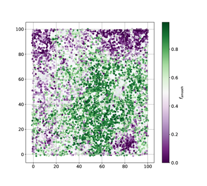
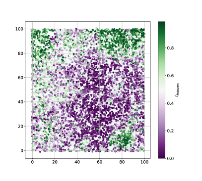
Figure 13: The fraction of GalaxyZoo votes in favor of a smooth galaxy, likely an elliptical, (right), and the voting fraction in favor of a galaxy with “features", likely a spiral galaxy (left). The votes are complementary identifying a smooth population over the center of the SOM with several features galaxy populations in the corners. The only other choice was “artifact".

The very first question in GalaxyZoo is whether the object has features, looks smooth or appears to be a star or artifact. Figure 13 shows the voting fractions in favor of a smooth galaxy and those in favor of a galaxy having “features". With Sérsic profile information as part of the feature space, one would expect a segregation of smooth (elliptical) galaxies and disk (featured) galaxies. The SOM voting in Figure 13 does show a reasonable separation in smooth and “featured" galaxies.

Our sample is low-redshift and should be well resolved in the KiDS images used for the GalaxyZoo. Other, smaller features, such as whether a galaxy has spiral arm structure or a bar, do not show as much separation on the $100\times 100$ SOM. The feature space of stellar mass ($M_{*}$), colour (u-r), specific star-formation rate (SSFR), Sérsic index ($n$), and half-light radius ($r_{50}$) does not discriminate well to cleanly isolate such features. A different feature space is needed for the separation of sub-galaxy scale morphological structures.

6 Concluding Remarks

We have mapped the feature space of a sample of nearly 8000 GAMA galaxies from Turner et al. (2019) onto a Self-Organizing Map to explore the success of K-means clustering on a galaxy sample, the green valley of galaxies, and some morphological features identified by the Galaxy Zoo. We opted for a 100$\times$100 node SOM. This size SOM was sufficient to separate out populations in this sample and the feature space contained enough resolution to do so (see Figure 8, 6, and 12).

Our first result is to compare the K-means clustering and Self-Organizing Maps, which are both instances of unsupervised learning on the entire dataset without necessarily splitting it into training and test or validation samples. The SOM application is a relatively straightforward comparison with the existing classifications from Turner et al. (2019). From their mapping onto our SOM, the K-means clustering using three (K3) or five (K5) clusters seem good descriptions, resolving into clear and continuous regions on the SOM (Figure 8). A higher number of clusters (K6) appear to be somewhat of an over-fit. However, the evaluation is still based on the visual interpretation of the SOM and remains a subjective one.

We note here that the GAMA data is not ideal K-means clustering data with an unequal distribution distance between peaks and clear elongation rather than isomorphic clusters. The result from Turner et al. (2019) stands: one needs more than a single bimodality in the galaxy population, manifesting in each feature (k2), to explain the bimodalities seen in single feature distributions. This is reflected in their Silhouette Coefficients as well (Table 1).

Secondly, we use two definitions of a traditional classification in a part of our feature space: the division into red and blue galaxies with the green valley in between based on $u-r$ colour and on specific star-formation. Green valley galaxies are indeed an interstitial population but not a single coherent one; several small green sub-populations are scattered throughout the SOM. Even using the general galaxy-wide properties the green valley population is spread to several different parts of the map (Figures 9 and 11). Blue and red galaxies separate based on the feature space into a single almost coherent grouping (albeit a complex shape) on the SOM. The green valley galaxies are a few nodes between the two dominating populations. We argue that this is consistent with the green valley being made up of several interstitial sub-populations, each quite distinct. Some may indeed be transitioning from blue to red (or the reverse) and some are not (consistent with Taylor et al., 2011; Schawinski et al., 2014). Especially notable is that low-mass green valley galaxies are mixed in with the other lower mass galaxies (Figure 10) consistent with these being much more alike then they are at higher masses.

Our final SOM experiment is to evaluate if the galaxy-wide feature space ($M_{*}$, $SSFR$, $u-r$, Sérsic $n$ and $r_{50}$) can map morphological features, such as those expressed by GalaxyZoo labels.

As a proof of concept, the first GalaxyZoo question (smooth or featured?) voting pattern for these galaxies does appear to segregate well on the SOM. Further GalaxyZoo questions hardly show any separation (e.g. the presence of a bar or spiral structure) which dominate in featured galaxies. Detailed morphologies on the kpc scale (bulges, spiral arms, and bars) are not well separated by this SOM map using the general galaxy properties feature space ($M_{*}$, $SSFR$, $u-r$, Sérsic $n$ and $r_{50}$). A different feature space is needed to classify to this detail.

A Self Organizing Map looks to be a promising tool to identify known and unknown populations in galaxy catalog feature space. The sub-populations in the green valley are our first example of that. We note that a slightly wider SOM than recommended aids with the separation of such sub-groupings. The hope for future applications is to identify instructive sub-populations in galaxy surveys using this mapping technique.

6.1 Data availability

We use the data-tables of the feature space and the K-means labels from Turner et al. (2019), derived from the GAMA DR3 (Baldry et al., 2018, http://www.gama-survey.org/dr3/) DMUs (SersicCatSDSS Kelvin et al., 2012), (MagPhys, S. Driver), based on LAMBDAR photometry (LambdarPhotometry Wright et al., 2016), and the minisom (Vettigli, 2019) package and examples.

7 Acknowledgements

BWH is supported by an Enhanced Mini-Grant (EMG). The material is based upon work supported by NASA Kentucky under NASA award No: 80NSSC20M0047.

AHW is supported by an European Research Council Consolidator Grant (No. 770935). MB is supported by the Polish National Science Center through grants no. 2020/38/E/ST9/00395, 2018/30/E/ST9/00698 and 2018/31/G/ST9/03388, and by the Polish Ministry of Science and Higher Education through grant DIR/WK/2018/12.

This research made use of Astropy, a community-developed core Python package for Astronomy (Astropy Collaboration et al., 2013, 2018).

Appendix A Feature Space mapped onto the SOM

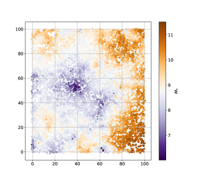
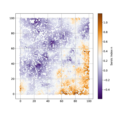
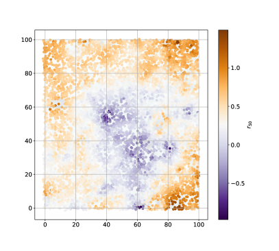
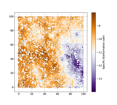
Figure 14: The absolute values of the feature space as mapped on the SOM. Compare to the weighting in Figure 5.

References

- Astropy Collaboration et al. (2013) Astropy Collaboration et al., 2013, A&A, 558, A33
- Astropy Collaboration et al. (2018) Astropy Collaboration et al., 2018, AJ, 156, 123
- Baldry et al. (2006) Baldry I. K., Balogh M. L., Bower R. G., Glazebrook K., Nichol R. C., Bamford S. P., Budavari T., 2006, MNRAS, 373, 469
- Baldry et al. (2010) Baldry I. K., et al., 2010, MNRAS, 404, 86
- Baldry et al. (2018) Baldry I. K., et al., 2018, MNRAS, 474, 3875
- Ball et al. (2008) Ball N. M., Loveday J., Brunner R. J., 2008, MNRAS, 383, 907
- Belfiore et al. (2017) Belfiore F., et al., 2017, MNRAS, 466, 2570
- Bluck et al. (2020) Bluck A. F. L., et al., 2020, MNRAS, 499, 230
- Brammer et al. (2009) Brammer G. B., et al., 2009, ApJ, 706, L173
- Bremer et al. (2018) Bremer M. N., et al., 2018, MNRAS, 476, 12
- Cheng et al. (2021) Cheng T.-Y., Huertas-Company M., Conselice C. J., Aragón-Salamanca A., Robertson B. E., Ramachandra N., 2021, MNRAS, 503, 4446
- Conselice (2006) Conselice C. J., 2006, MNRAS, 373, 1389
- Davidzon et al. (2019) Davidzon I., et al., 2019, MNRAS, 489, 4817
- Driver et al. (2006) Driver S. P., et al., 2006, MNRAS, 368, 414
- Driver et al. (2009) Driver S. P., et al., 2009, Astronomy and Geophysics, 50, 050000
- Driver et al. (2016) Driver S. P., et al., 2016, ApJ, 827, 108
- Faber et al. (2007) Faber S. M., et al., 2007, ApJ, 665, 265
- Fernandez et al. (2021) Fernandez J., Alonso S., Mesa V., Duplancic F., Coldwell G., 2021, arXiv e-prints, p. arXiv:2107.06920
- Géron et al. (2021) Géron T., Smethurst R. J., Lintott C., Kruk S., Masters K. L., Simmons B., Stark D. V., 2021, MNRAS, 507, 4389
- Graham (2019) Graham A. W., 2019, MNRAS, 487, 4995
- Graham et al. (2006) Graham A. W., Merritt D., Moore B., Diemand J., Terzić B., 2006, AJ, 132, 2711
- Hemmati et al. (2019) Hemmati S., et al., 2019, ApJ, 881, L14
- Holwerda et al. (2019) Holwerda B. W., et al., 2019, AJ, 158, 103
- Kelvin et al. (2012) Kelvin L. S., et al., 2012, MNRAS, 421, 1007
- Kelvin et al. (2014) Kelvin L. S., et al., 2014, MNRAS, 439, 1245
- Kelvin et al. (2018) Kelvin L. S., et al., 2018, MNRAS, 477, 4116
- Kennedy et al. (2015) Kennedy R., et al., 2015, MNRAS, 454, 806
- Kennedy et al. (2016a) Kennedy R., et al., 2016a, MNRAS, 460, 3458
- Kennedy et al. (2016b) Kennedy R., Bamford S. P., Häußler B., Brough S., Holwerda B., Hopkins A. M., Vika M., Vulcani B., 2016b, A&A, 593, A84
- Kohonen (2001) Kohonen T., 2001, Self-organizing maps. Self-organizing maps. 3rd ed. Berlin: Springer, 2001, xx, 501 p. Springer series in information sciences, ISBN 3540679219
- Kuijken et al. (2019) Kuijken K., et al., 2019, A&A, 625, A2
- Lintott et al. (2008) Lintott C. J., et al., 2008, MNRAS, 389, 1179
- Liske et al. (2015) Liske J., et al., 2015, MNRAS, 452, 2087
- Masters et al. (2010) Masters K. L., et al., 2010, MNRAS, 405, 783
- Moffett et al. (2016a) Moffett A. J., et al., 2016a, MNRAS, 457, 1308
- Moffett et al. (2016b) Moffett A. J., et al., 2016b, MNRAS, 462, 4336
- Moutard et al. (2016) Moutard T., et al., 2016, A&A, 590, A103
- Naim et al. (1997) Naim A., Ratnatunga K. U., Griffiths R. E., 1997, ApJS, 111, 357
- Noeske et al. (2007) Noeske K. G., et al., 2007, ApJ, 660, L43
- Phillipps et al. (2019) Phillipps S., et al., 2019, MNRAS, 485, 5559
- Rowlands et al. (2018) Rowlands K., et al., 2018, MNRAS
- Salim (2015) Salim S., 2015
- Scarlata et al. (2007) Scarlata C., et al., 2007, ApJS, 172, 406
- Schawinski et al. (2014) Schawinski K., et al., 2014, MNRAS, 440, 889
- Sérsic (1963) Sérsic J. L., 1963, Boletin de la Asociacion Argentina de Astronomia La Plata Argentina, 6, 41
- Sérsic (1968) Sérsic J. L., 1968, Atlas de galaxias australes
- Smethurst et al. (2015) Smethurst R. J., et al., 2015, MNRAS, 450, 435
- Smethurst et al. (2017) Smethurst R. J., Lintott C. J., Bamford S. P., Hart R. E., Kruk S. J., Masters K. L., Nichol R. C., Simmons B. D., 2017, MNRAS, 469, 3670
- Taylor et al. (2011) Taylor E. N., et al., 2011, MNRAS, 418, 1587
- Taylor et al. (2015) Taylor E. N., et al., 2015, MNRAS, 446, 2144
- Turner et al. (2019) Turner S., et al., 2019, MNRAS, 482, 126
- Turner et al. (2021) Turner S., et al., 2021, MNRAS, 503, 3010
- Vettigli (2019) Vettigli G., 2019, MiniSom: minimalistic and NumPy-based implementation of the Self Organizing Map, GitHub.[Online]. Available: https://github.com/JustGlowing/minisom/
- Vulcani et al. (2014) Vulcani B., et al., 2014, MNRAS, 441, 1340
- Wang et al. (2016) Wang L., et al., 2016, MNRAS, 461, 1898
- Weigel et al. (2017) Weigel A. K., et al., 2017, ApJ, 845, 145
- Willmer et al. (2006) Willmer C. N. A., et al., 2006, ApJ, 647, 853
- Wright et al. (2016) Wright A. H., et al., 2016, MNRAS, 460, 765
- York et al. (2000) York D. G., et al., 2000, AJ, 120, 1579
- da Cunha et al. (2008) da Cunha E., Charlot S., Elbaz D., 2008, MNRAS, 388, 1595
- de Jong et al. (2013) de Jong J. T. A., Verdoes Kleijn G. A., Kuijken K. H., Valentijn E. A., 2013, Experimental Astronomy, 35, 25
- de Jong et al. (2015) de Jong J. T. A., et al., 2015, A&A, 582, A62
- de Jong et al. (2017) de Jong J. T. A., et al., 2017, A&A, 604, A134