Estimating Nonlinear Network Data Models with Fixed Effects

Abstract

I introduce a new method for bias correction of dyadic models with agent-specific fixed-effects, including the dyadic link formation model with homophily and degree heterogeneity. The proposed approach uses a jackknife procedure to deal with the incidental parameters problem. The method can be applied to both directed and undirected networks, allows for non-binary outcome variables, and can be used to bias correct estimates of average effects and counterfactual outcomes. I also show how the jackknife can be used to bias-correct fixed effect averages over functions that depend on multiple nodes, e.g. triads or tetrads in the network. As an example, I implement specification tests for dependence across dyads, such as reciprocity or transitivity. Finally, I demonstrate the usefulness of the estimator in an application to a gravity model for import/export relationships across countries.

1 Introduction

Networks are common in both economic and social contexts, and it is important to understand the factors that play a role in both the formation and strength of the links between agents. The econometric analysis of networks faces a number of challenges that have received much attention in recent literature (see de Paula (2020) and Graham (2020) for reviews of this literature). One common modeling approach is to assume a dyadic network structure (one in which decisions are made bilaterally between agents), but allow for linking decisions to depend on unobserved agent-specific heterogeneity. These models are common in practice since they are straightforward to implement while still being able to capture important aspects of observed networks. Controlling for agent-specific heterogeneity is important since in many real world networks agents vary significantly in the number and strength of connections made. Ignoring this heterogeneity can lead to large biases in estimated effects.

In this paper, I consider the estimation of dyadic models, where the presence of unobserved heterogeneity is accounted for by two sets of agent-specific fixed effects – a sender and a receiver effect. The fixed effects approach is appealing as it does not require strong assumptions about the unobserved component as in random effects models. In addition, the network setting does not suffer from the ‘fixed $T$’ issues of panel data, since we observe every agent interacting with $N-1$ other agents in the network, so that fixed effect estimates are consistent. However, the large number of fixed effects (proportional to the square root of the sample size) does create an incidental parameter problem (Neyman and Scott, 1948). This paper proposes a jackknife approach to bias correction, which has a number of benefits over existing methods. Importantly, the jackknife is easily adaptable to a range of settings, including models for non-binary outcome variables. Additionally, since the jackknife estimates all of the parameters in the model, including the fixed effects, it is possible to construct estimates of average effects and counterfactual outcomes. I also show how the jackknife can be used to bias correct averages over functions of multiple observations (e.g. dyads or triads in the network), which I show is useful for constructing specification test statistics, such as tests for the presence of certain strategic interactions like reciprocity or transitivity.

I demonstrate the consistency and asymptotic normality of the jackknife estimator under asymptotic sequences in which a single network grows in size, while the network remains ‘dense’. The network model I consider is one in which agents make bilateral decisions about link-specific outcomes, independently of other relationships. This type of dyadic model (a dyad is a pair of agents) has received much attention in the literature, because of its tractability and its ability to replicate some key features of observed networks. In particular, it allows for: homophily, the tendency of agents to form stronger ties with other agents that are similar to them; and degree heterogeneity, where the number/strength of links in the networks can vary substantially across nodes.

In the case of a binary outcome variable, the model I consider is one of link formation, and is an extension of the model by Holland and Leinhardt (1981). There are several alternative approaches to address the incidental parameters problem in this setting. Graham (2017), Charbonneau (2017), and Jochmans (2018) all consider versions of this model in which the latent disturbances follow a logistic distribution, and use conditioning arguments to remove dependence on the fixed effects. The conditioning approach has the advantage of being applicable under certain sparse network asymptotic sequences, but is limited to models in which sufficient statistics for the fixed effects exist, and is not able to recover counterfactuals or average effects. Yan et al. (2019) also studies the logistic model and provides asymptotic results for the incidental parameters. Graham (2017) considers an analytical correction for the logistic model, while Dzemski (2019) derives the analytical correction for a probit model. The analytical bias correction approach is limited to dense network sequences, as in this paper, and similarly to this paper can recover average effects. The advantage of the jackknife correction relative to an analytical approach is that it provides an off-the-shelf approach that researchers may apply to new settings, without the need to first derive bias expressions. Candelaria (2020), (Toth, 2017), and Gao (2020) study identification of the common parameters without a known parametric form for the disturbance term, while Zeleneev (2020) allows for nonparametric structure in the unobserved heterogeneity term.

Although the focus of the literature on dyadic network models has been on the binary outcome case, researchers often have access to outcome variables that are non-binary. Examples of these settings include the value of exports between countries, the value of loans between banks, or the number of workers migrating between states. The results in this paper are derived for a general M-estimator satisfying basic regularity conditions and so cover a range of models for both binary and non-binary outcome variables, as well as a range of estimation approaches, including MLE, quasi-MLE and nonlinear least squares estimation.

As a demonstration of the technique in an empirical setting, I estimate a model of international trade relationships. Gravity models have been a workhorse model in the trade literature for many years, and the importance of including country-specific fixed effects is well known ((Anderson and Van Wincoop, 2003)). I demonstrate the importance of bias correction in estimates of a probit model for the formation of country-level trade relationships. The bias correction changes the value of some estimated coefficients and marginal effects by more than a standard deviation in magnitude.

The jackknife bias correction also allows for the construction of various specification tests. Many models of network formation include strategic aspects in which agents’ decisions are influenced by the state of the network. For instance, agent $i$ may find it more beneficial to link with $j$ if they already share many other links in common. Graham and Pelican (2020) derives the locally best similar test for a class of alternatives in a logit model, using conditioning arguments. Dzemski (2019) tests for the presence of transitive links with triads (groups of three agents) in a probit model, and derives an analytical bias correction for the statistic. I demonstrate that a range of test statistics, including that of Dzemski (2019), can be bias-corrected using the jackknife. This extends the set of tests available to researchers, as well as the range of models they can be applied to. As an example, I test for transitivity in both a country-level trade network, and a network of professional friendships. I find no evidence of excess transitivity in the trade network (although the uncorrected statistic would lead to the opposite conclusion), while the social network appears to display strong transitivity.

The network jackknife extends previous results on jackknife bias correction in panel data. Hahn and Newey (2004) introduced a jackknife correction for panel estimators with individual fixed effects, based on re-estimating the parameters on data sets that exclude a single time period. Dhaene and Jochmans (2015) present a split-sample version of this idea based on estimating the model in the first and second halves of time periods separately. Fernández-Val and Weidner (2016) develop a general framework that allows for both time and individual fixed effects. The analysis in this paper builds heavily off of the asymptotic expansions in Fernández-Val and Weidner (2016).

Analogously to the panel data setting, the network jackknife is constructed by forming ‘leave-out’ estimates that exclude certain subsets of the data. Cruz-Gonzalez et al. (2017) and Chen et al. (2021) have suggested jackknife approaches for network data, although without formal proof, based on either a split-sample approach or a leave-one-out approach that drops a single agent at a time. I propose a different approach to jackknifing network data that is based on a novel partitioning of the data set that constructs leave-out estimates that remove bias from both sender and receiver of fixed effects in one step. I extend the asymptotic expansions of Fernández-Val and Weidner (2016) to allow for formal analysis of the jackknife estimator. The jackknife proposed here drops a single observation per fixed effect at each step, so that it is likely to have better finite sample variance properties than the split-sample approach (see Hahn et al. (2023) for a formal argument in the panel setting). In contrast to a jackknife that drops all observations from a single agent in the network, our jackknife retains all agents in each leave-out estimation, so that the distribution of unobserved effects is held constant. I demonstrate the small-sample effectiveness of our approach in comparison to previous suggestions in simulations that show that our jackknife is more robust to settings with meaningful levels of unobserved heterogeneity and in networks with lower density.

The rest of the paper is organized as follows. Section 2 introduces the network model, Section 3 discusses implementation of the jackknife procedure for the estimation of model parameters, while Section 4 discusses estimation of average effects, and the construction of specification tests. In Section 5 I demonstrate the method by estimating a model of international trade flows, while Section 6 reports simulation results that are consistent with the jackknife theory.

2 The dyadic linking model

The researcher observes a network of $N$ agents, which may be individuals, firms, countries, and so on. For each of the $N(N-1)/2$ pairs of agents $(i,j)$, called a dyad, we observe the outcome of two directed linking decisions $Y_{ij}$ and $Y_{ji}$. The network may be directed, in which case $Y_{ij}\neq Y_{ji}$ in general, or undirected, in which case the two outcomes are equal. Following the literature, I term $i$ the ‘sender’ and $j$ the ‘receiver’ in link $Y_{ij}$. The outcome variable $Y_{ij}$ may be binary, capturing the presence (or absence) of a link between two agents, or may represent a measure of the strength of the link between agents, in which case $Y_{ij}$ is non-binary. For example, $Y_{ij}$ may be the value of exports from country $i$ to country $j$ in a particular year, or the number of times agents $i$ and $j$ interacted in some period.

The researcher additionally observes a set of link-specific covariates $X_{ij}$, which capture determinants of linking decisions such as homophily, the tendency for agents to link with other agents that are similar to themselves. Agents are endowed with two fixed effects, $\alpha_{i}$ and $\gamma_{i}$, which capture unobserved degree heterogeneity, that is, the tendency of some agents to form more (or stronger) links than others. The ‘sender’ fixed effect $\alpha_{i}$ accounts for heterogeneity in out-degree (the number or strength of links from agent $i$ to other agents), while the ‘receiver’ fixed effect accounts for in-degree heterogeneity. Degree heterogeneity is an important feature of many networks, for example, we would expect countries with larger GDPs to engage in more trade than smaller countries ceteris paribus (see Anderson and Van Wincoop (2003) for an example of such a model). Graham (2017) provides intuition for why failing to account for degree heterogeneity can bias conclusions about homophily in a network. The fixed effects will be treated as unknown parameters in the model, and the researcher does not need to specify their distribution or how they relate to the covariates.

The data $(Y_{ij},X_{ij})$ are assumed to be drawn from some model, which I leave unspecified but assume that we are able to identify the model parameters $(\beta_{0},\alpha_{0},\gamma_{0})$ as solutions to the population maximization problem

$$\max_{(\beta,\alpha,\gamma)\in\mathbb{R}^{\dim\beta+2N}}\bar{E}\big{[}\mathcal{L}_{N}(\beta,\alpha,\gamma)\big{]},$$

$$\mathcal{L}_{N}(\beta,\alpha,\gamma)=\frac{1}{N-1} \sum_{i}\sum_{j\neq i}\ell(Y_{ij},X_{ij},\beta,\alpha_{i}+\gamma_{j})-\frac{b}{2N}\big{(}\sum_{i}\alpha_{i}-\sum_{i}\gamma_{i}\big{)}^{2},$$ (1)

where $\bar{E}$ represents expectation conditional on the fixed effects, and $\ell$ is a known function that is maximized in expectation at the true parameters. The objective function in (1) covers many common models including MLE, quasi-MLE, and nonlinear least squares estimators.

Example (Maximum likelihood).

If we specify the full conditional distribution of the outcome variable as $Y_{ij}|X,\beta,\alpha,\gamma\sim f(Y_{ij}|X_{ij},\beta,\alpha_{i}+\gamma_{j})$, then $\mathcal{L}(\beta,\alpha,\gamma)$ will be the log-likelihood function. An important example is a model of directed link formation according to

$$Y_{ij} =\mathds{1}\{X_{ij}^{\prime}\beta+\alpha_{i}+\gamma_{j}-\varepsilon_{ij}\geq 0\},$$ (2)

where $\varepsilon_{ij}$ follows a known distribution $F$. This is an extension of the linking model of Holland and Leinhardt (1981) and has been used extensively in empirical literature.

Example (Nonlinear least squares).

The researcher may choose to specify only the conditional mean function for the outcome, rather than its full distribution, e.g $E\big{[}Y_{ij}|X,\beta,\alpha,\gamma\big{]}=h(X_{ij},\beta,\alpha_{i}+\gamma_{j})$. In this case, we may estimate the parameters of the model by setting $\ell(Y_{ij},X_{ij},\beta,\alpha_{i}+\gamma_{j})=-\big{(}Y_{ij}-h(X_{ij},\beta,\alpha_{i}+\gamma_{j})\big{)}^{2}$.

The unobserved effects are assumed to enter in an additively separable manner, i.e. as $\alpha_{i}+\gamma_{j}$,and so identification of the two sets of fixed effects parameters requires a normalization, for which we choose $\sum_{i}\alpha_{i}=\sum_{i}\gamma_{i}$. The term $\frac{b}{2N}\big{(}\sum_{i}\alpha_{i}-\sum_{i}\gamma_{i}\big{)}^{2}$ is a penalty term intended to impose this normalization on the fixed effect parameters, where $b>0$ as an arbitrary constant. Note that the vectors of fixed effects $\alpha$ and $\gamma$ are dependent on the network size $N$, although I leave this dependence implicit in the notation. When functions are evaluated at the true parameters $(\beta_{0},\alpha_{0},\gamma_{0})$ I will typically drop them from notation. I will also use the shorthand $\ell_{ij}=\ell(Y_{ij},X_{ij},\beta_{0},\alpha_{0,i}+\gamma_{0,j})$ when convenient.

Model assumptions

We will impose two key assumptions on the structure of the network.

Assumption 1.

(i) Conditional on $(X,\alpha,\gamma)$, dyads are independent, i.e.

$$Y_{ij}\mathchoice{\mathrel{\hbox to0.0pt{$\displaystyle\perp$\hss}\mkern 2.0mu{\displaystyle\perp}}}{\mathrel{\hbox to0.0pt{$\textstyle\perp$\hss}\mkern 2.0mu{\textstyle\perp}}}{\mathrel{\hbox to0.0pt{$\scriptstyle\perp$\hss}\mkern 2.0mu{\scriptstyle\perp}}}{\mathrel{\hbox to0.0pt{$\scriptscriptstyle\perp$\hss}\mkern 2.0mu{\scriptscriptstyle\perp}}}Y_{kl}|X,\beta,\alpha,\gamma\quad\quad\forall(k,l)\notin\{(i,j),(j,i)\}.$$ (3)

(ii) Let $\mathcal{B}_{\varepsilon}$ be an $\varepsilon$-neighborhood that contains $(\beta_{0},\alpha_{i},\gamma_{j})$ for all $(i,j)$. There exist constants $b_{min}$ and $b_{max}$ such that for all $(\beta,\pi)\in\mathcal{B}_{\varepsilon}$

$$0<b_{min}\leq-\bar{E}[\partial_{\pi^{2}}\ell_{ij}(\beta,\pi)]\leq b_{max}$$

a.s. uniformly over $i,j$ and $N$.

Assumption 1 (i) implies that linking decisions are bilateral in nature. This assumption does allow for dependence between the two links within a pair of agents (a dyad), but implies the decision between $i$ and $j$ is independent of that between $i$ and $k$ for instance. Importantly, this independence is conditional on the covariates and agent-specific fixed effects. Unconditionally, country $i$’s exports to country $j$ are correlated with their exports to country $k$, since both are determined by the exporter effect $\alpha_{i}$. In many settings, the inclusion of fixed effects will be important in establishing the plausibility of conditional independence. Assumption 1 (i) may not be appropriate in situations where linking decisions are strategic. Estimation of models with strategic interactions is substantially more challenging, and is likely to require multiple observations of the network over time. Nonetheless, the dyadic model presented here still represents an important baseline model, and can be used to construct tests for the presence of strategic interactions against the null hypothesis of (3). We discuss examples of such tests in Section 4.2.

Assumption 1 (ii) ensures that the Hessian for the fixed effect parameters is positive definite. This requires sufficient variation in the outcomes across both dimensions i.e., variation in $Y_{ij}$ over $j$ (for fixed sender $i$) and over $i$ (for fixed receiver $j$). In the binary outcome case, it implies that the model generates a dense network, one in which the number of links formed by each node tends to infinity as the size of the network grows. The assumption may not be reasonable in all empirical settings – in simulations we investigate the robustness of the estimator to sparsity in finite samples. However, it seems a natural condition when we hope to estimate parameters that depend on the unobserved heterogeneity, such as marginal effects or counterfactual outcomes.

Incidental parameters problem

As is well known, nonlinear estimators with fixed effects suffer from an incidental parameter problem (Neyman and Scott, 1948). In total, the model contains $\dim(\beta)+2N$ parameters to be estimated, from the $N(N-1)$ observations $(Y_{ij},X_{ij}^{\prime})$ — we will typically refer to these observations using the shorthand $(i,j)$. Briefly, since the first-order condition for the fixed effect $\alpha_{i}$ depends only on the $N-1$ observations $(i,j)$ for $j\neq i$, estimation of the fixed effects results in a bias of order $O(N^{-1})$. Under regularity conditions discussed in Section 3.2, we can show that the bias of the maximizer of the profile objective function (concentrating out the fixed effect parameters) is approximately given by

$$\beta_{N}-\beta_{0}\approx\frac{B_{N}}{N-1}$$ (4)

This bias is of the same order as the standard error for estimation of the common parameter $\beta$ (recall that $N$ is the square-root of the sample size). Since the bias $\beta_{N}-\beta_{0}$ is of the same order as the estimation error, $O(N^{-1})$, $\widehat{\beta}$ will be asymptotically biased, that is

$$N(\widehat{\beta}-\beta_{0})\Rightarrow\mathcal{N}\big{(}B,V\big{)}.$$

for some bias term $B_{N}$.

The incidental parameters generate an asymptotic bias in the network model analogous to the panel setting with both $N$ and $T$ growing to infinity at the same rate. Hahn and Newey (2004) derive asymptotic expansions for models with individual fixed effects, while Fernández-Val and Weidner (2016) derive expansions that apply to general models with additively separable unobserved effects, and Chen et al. (2021) consider the setting with interactive effects. The results in this paper rely on similar expansions, which build on this prior work. Dzemski (2019) also applies the Fernández-Val and Weidner (2016) expansions to the network model structure to derive bias expressions for a probit model. In this paper, we extend the asymptotic expansions to higher order so that they may be used to justify jackknife bias correction procedures. We demonstrate that, under mild additional regularity conditions, the incidental parameters bias can be corrected using a jackknife estimator.

3 Jackknife bias correction

3.1 Jackknife for dyadic data

The jackknife bias-corrected estimator is constructed as a linear combination of the full-sample parameter estimates and an average of ‘leave-out’ estimators that exclude certain observations in the data set. The particular linear combination chosen can be motivated by asymptotic expansions of the estimator, in particular the form of the bias in (4).

Suppose we were to drop observations from our data set in such a way that for every agent $i$ we exclude one observation in which $i$ is the sender, and one observation in which $i$ is the receiver (recall that a single observation is a directed $(i,j)$ pair, of which we observe $N(N-1)$ in total). We show that the new estimator using this ‘leave-out’ sample, $\tilde{\beta}$, has a bias that is approximately

$$\bar{E}[\tilde{\beta}]-\beta\approx\frac{B_{N}}{N-2}.$$

The form of the bias for $\tilde{\beta}$ can be explained by two important factors: (i) $\tilde{\beta}$ is estimated using only $N-2$ observations per fixed effect, since we excluded one observation related to each fixed effect parameter, and (ii) $\tilde{\beta}$ is estimated on a random sample generated from the same set of fixed effects, so that the bias expression $B_{N}$ is the same as that in (4).

Taking advantage of the fact that the estimate $\tilde{\beta}$ has a larger bias than the full-sample estimate $\widehat{\beta}$ by the factor $\frac{N-1}{N-2}$, we can construct a new estimator $\widehat{\beta}_{jack}=(N-1)\widehat{\beta}-(N-2)\tilde{\beta}$ which has no asymptotic bias

$$\bar{E}\big{[}(N-1)\widehat{\beta}-(N-2)\tilde{\beta}\big{]}-\beta\approx 0.$$

To describe the construction of the leave-out estimators, we first define a partition of the $N(N-1)$ observations of directed pairs $(i,j)$ into $N-1$ distinct sets

$$\mathcal{I}_{k}=\big{\{}(1,1+k),\dots,(N-k,N),(N-k+1,1),\dots,(N,k)\big{\}},$$

for $k=1,\dots,N-1$. We define the $k$-th ‘leave-out sample’ to be the set of observations that excludes the observations $(i,j)\in\mathcal{I}_{k}$.

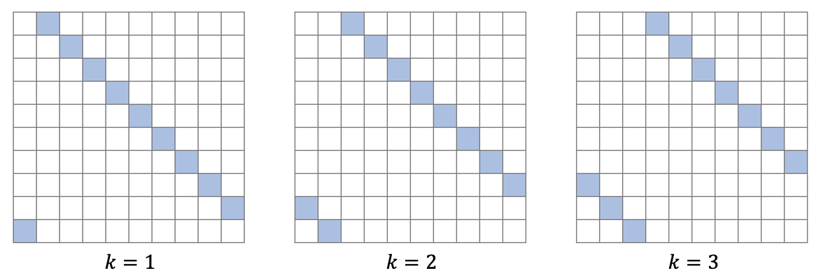
Figure 1: Diagram of the sets $\mathcal{I}_{k}$ for $k=1,2,3$.

Observation $(i,j)$ in the network is represented by the corresponding position in each matrix. The shaded squares are the observations contained in the leave-out sets $\mathcal{I}_{k}$

Figure 1 represents the structure of the first three sets $\mathcal{I}_{k}$ for a network of $N=10$ agents. Observations are ordered in an $N\times N$ matrix so that the $(i,j)$ cell represents the corresponding observation in the network (the diagonal elements are empty since there are no $(i,i)$ observations). The leave-out sets take diagonal slices from the data matrix. Importantly, constructing the sets this way ensures that each contains exactly one observation related to each sender and receiver fixed effect, i.e. there is one observation taken from every row and every column of the data matrix.

Let $1_{ij}^{k}=\mathds{1}\{(i,j)\not\in\mathcal{I}_{k}\}$, be an indicator variable that is equal to one whenever the observation $(i,j)$ is in the $k$-th leave-out sample. The $k$-th leave-out estimates are

$$(\widehat{\beta}_{(k)},\widehat{\phi}_{(k)}) =\operatorname*{arg\,max}_{(\beta,\phi)\in\mathbb{R}^{\dim(\beta)+2N}}\frac{1}{N-2}\sum_{i}\sum_{j\neq i}\ell_{ij}(\beta,\phi)\times\mathds{1}_{ij}^{k},$$

$$\text{subject to }\sum_{i}\alpha_{i}=\sum_{i}\gamma_{i},$$

that is, the estimates obtained by excluding the observations in $\mathcal{I}_{k}$ from the data. We can then construct the jackknife bias-corrected estimator

$$\widehat{\beta}_{J}=(N-1)\widehat{\beta}_{N}-(N-2)\frac{1}{N-1}\sum_{k=1}^{N-1}\widehat{\beta}_{(k)}.$$ (5)

The construction of the leave-out estimators is analogous to jackknife bias correction in the panel data setting; however, the structure of the jackknife proposed here is new. The procedure relies on dropping sets of observations that contain a single observation related to every sender fixed effect $\alpha_{i}$ as well as every receiver fixed effect $\gamma_{i}$. In this way, the bias from both types of fixed effects can be addressed simultaneously, while holding the distribution of fixed effects constant across the leave-out samples. This is in contrast to an approach which drops all observations from a single agent, which removes that agents’ fixed effects from the leave-out sample and alters the distribution of unobserved heterogeneity. We provide simulation evidence that the method proposed here is more robust to networks that have more unobserved heterogeneity or are less dense.

We prove in Section 3.2 that the jackknife bias correction is consistent, and asymptotically normal, with mean zero and variance equal to that of the full-sample estimate

$$N(\widehat{\beta}_{J}-\beta_{0})\Rightarrow\mathcal{N}\big{(}0,V\big{)}.$$

The fact that the jackknife is able to remove bias without affecting the asymptotic variance of the estimator may seem surprising. This important feature is achieved by averaging across the $N-1$ different leave-out estimators $\widehat{\beta}_{(k)}$. Since the sets $\mathcal{I}_{1},\dots,\mathcal{I}_{N-1}$ form a partition of the $N(N-1)$ observations in the network, each observation is excluded from exactly one of the leave-out estimates. This balanced treatment of observations ensures that the jackknife procedure does not affect the first-order asymptotic approximation of the estimator.

Remark 1.

The construction of the sets $\mathcal{I}_{k}$ depends on the labelling of nodes, and so the final estimator will be dependent on this labelling (since the make-up of the leave-out samples will change). Some of the arbitrariness of this labelling could be removed by re-randomizing the node labels and averaging over the resulting estimates. In practice the estimators with different labelings are likely to be highly similar so that the additional computations will have little effect, although it may be useful to try some alternative labellings to confirm this in applications.

The jackknife estimator requires $N$ estimations of the model, and so may be computationally intensive for large networks, although speed may be improved by computing the leave-out estimates in parallel, and using good starting values such as the full sample estimates. As an alternative, we present a ‘leave-$l$-out’ version of the jackknife, which reduces the number of additional estimations of the model by dropping $l$ observations per fixed effect, as opposed to just one. To describe the estimator, let $N_{l}=\frac{N-1}{l}$ (we assume here that $N-1$ is divisible by $l$ for simplicity). We can construct a partition of the data into $N_{l}$ non-overlapping sets $\mathcal{I}_{k}^{l}$, defined by combining $l$ of the original sets as follows $\mathcal{I}_{k}^{l}=\cup_{j=0}^{l-1}\mathcal{I}_{k+jN_{l}}$, for $k=1,\dots,N_{l}$. This results in $N_{l}$ leave-$l$-out samples, with corresponding estimates $\hat{\beta}_{l,(k)}$, which are the estimates from using all observations except those in the $k$-th set $\mathcal{I}_{k}^{l}$. A jackknife bias-corrected estimate can then be constructed as

$$\hat{\beta}_{J,l}=\frac{N-1}{l}\hat{\beta}_{N}-\frac{N-1-l}{l}\frac{1}{N_{l}}\sum_{k=1}^{N_{l}}\hat{\beta}_{l,(k)}.$$ (6)

Remark 2.

The leave-$l$-out jackknife bias correction has the same asymptotic variance as the standard leave-one-out jackknife and the full-sample estimator. However, there may be some finite-sample efficiency loss, particularly when $l$ is large or when the network is not sufficiently dense. Hahn et al. (2023) show in the panel case that the leave-one-out jackknife has smaller higher-order variance and bias than the split-sample jackknife (i.e. its variance to $O(N^{-1})$ is smaller), and it is likely that the same result applies here, although this is beyond the scope of the present paper.

3.2 Asymptotic analysis for the common parameters

Before stating the asymptotic result for the jackknife estimator for $\beta$, we first introduce some additional notation and state regularity conditions. We consider an asymptotic framework in which a single network of $N$ agents grows in size, i.e. $N\to\infty$. Recall that the parameters of interest maximize the objective function in (1) for some function $\ell_{ij}=\ell(Y_{ij},X_{ij},\beta,\alpha_{i}+\gamma_{j})$ of the observables $Z_{ij}=(Y_{ij},X_{ij})$ and additive unobserved fixed effects $\alpha_{i}+\gamma_{j}$. Denote the $2N\times 1$ vector of fixed effects by $\phi^{\prime}=(\alpha^{\prime},\gamma^{\prime})$ and let $\pi_{ij}=\alpha_{i}+\gamma_{j}$ represent the additive index through which they enter the objective function. We denote derivatives of the function $\ell$ with respect to parameters by $\partial_{\beta}\ell_{ij}(\beta,\alpha,\gamma)=\partial\ell_{ij}(\beta,\alpha,\gamma)/\partial\beta$, $\partial_{\pi^{q}}\ell_{ij}(\beta,\alpha,\gamma)=\partial^{q}\ell_{ij}(\beta,\alpha,\gamma)/\partial\pi^{q}$ etc. When evaluating these objects at the true parameter values, we simply write $\partial_{\pi^{q}}\ell_{ij}$ and so on. The corresponding derivatives of the objective function are denoted by $\partial_{\beta}\mathcal{L}=\frac{1}{N-1}\sum_{i}\sum_{j\neq i}\partial_{\beta}\ell_{ij}$, $\partial_{\phi\phi^{\prime}}\mathcal{L}=\frac{1}{N-1}\sum_{i}\sum_{j\neq i}\partial_{\phi\phi^{\prime}}\ell_{ij}$ etc. Finally, we denote expectations of objects (conditional on the fixed effects) by $\partial_{\beta}\bar{\mathcal{L}}=\bar{E}[\partial_{\beta}\mathcal{L}]$, and deviations from these expectations as $\partial_{\beta}\tilde{\mathcal{L}}=\partial_{\beta}\mathcal{L}-\bar{E}[\partial_{\beta}\mathcal{L}]$.

In addition to Assumption 1, we impose the following regularity conditions. The conditions are familiar conditions for M-estimators and follow the assumptions made in Fernández-Val and Weidner (2016) for example, which the exception of a strengthening of the requirements on smoothness and differentiabillity of the objective function, which are needed to justify the higher-order expansions of the jackknife estimator.

Assumption 2 (Regularity conditions).

Let $\varepsilon>0$. For every $(i,j)$ let $\mathcal{B}_{\varepsilon}$ be a subset of $\mathbb{R}^{\dim\beta+1}$ that contains an $\varepsilon$-neighborhood of $(\beta{}_{0},\pi_{0,ij})$ for all $N$ and all $(i,j)$.

(i) For all $i,j$ and $N$ we have that $\bar{E}[\partial_{\beta}\ell_{ij}]=\bar{E}[\partial_{\pi}\ell_{ij}]=0$. For all $N$, the objective function $\mathcal{L}$ is strictly concave over $\mathbb{R}^{\dim\beta+2N}$, and the matrix $\bar{\mathcal{H}}=-\partial_{\phi\phi^{\prime}}\bar{\mathcal{L}}$ is positive definite.

(ii) For all $(i,j)$, the function $(\beta,\pi)\mapsto\ell_{ij}(\beta,\pi)$ is five times continuously differentiable over $\mathcal{B}_{\varepsilon}$ almost surely. For all $(i,j)$, the partial derivatives of $\ell_{ij}$ with respect to the elements of $(\beta,\pi)$ up to fifth order are bounded in absolute value uniformly over $(\beta,\pi)\in\mathcal{B}_{\varepsilon}$ by a function $M(Z_{ij})>0$ a.s., where $\max_{i,j}\bar{E}[M(Z_{ij})^{16}]$ is a.s. uniformly bounded over $N$.

(iii) Let

$$\bar{W}_{N} =-\frac{1}{N}\big{(}\partial_{\beta\beta^{\prime}}\bar{\mathcal{L}}-(\partial_{\phi\beta^{\prime}}\bar{\mathcal{L}})(\partial_{\phi\phi^{\prime}}\bar{\mathcal{L}})^{-1}(\partial_{\beta\phi}\bar{\mathcal{L}})\big{)}$$

$$\bar{\Omega}_{N} =\bar{E}\big{[}\big{(}\partial_{\beta}\mathcal{L}-(\partial_{\beta\phi^{\prime}}\bar{\mathcal{L}})(\partial_{\phi\phi^{\prime}}\bar{\mathcal{L}})^{-1}(\partial_{\phi}\mathcal{L})\big{)}^{2}\big{]}.$$

The limits $\text{plim}_{N\to\infty}\bar{W}_{N}=W$ and $\text{plim}_{N\to\infty}\bar{\Omega}_{N}=\Omega$ exist for $W$ and $\Omega$ positive definite matrices.

Assumption 1(i) contains the parametric restriction of the model and requires that the true parameters $\beta_{0},\alpha_{0},\gamma_{0}$ are solutions to the first-order equations of the objective function. Concavity of the objective function ensures that the population problem has a unique solution. This is satisfied in many common nonlinear models, including the class of regression models with log-concave densities (as well as censored and truncated versions of these models), which includes probit, logit, ordered probit, Tobit, gamma and beta models among others (see Pratt (1981), Newey and McFadden (1994)).

Assumption 1(ii) provides basic smoothness conditions for the objective function. The derivative and moment conditions are required to ensure the validity of the asymptotic expansions to high enough order to establish the properties of the jackknife procedure, and to ensure that remainder terms are well bounded. Analysis of the jackknife requires higher order expansions than are required for characterization of the analytical bias and first-order asymptotic properties of the estimator, and so Assumption 1(ii) is somewhat stronger than the equivalent assumption employed in Fernández-Val and Weidner (2016).

Assumption 1(iii) ensures that the variance of $\widehat{\beta}$ is non-degenerate. The term $\bar{W}_{N}$ is the Hessian matrix for the common parameters $\beta$, after concentrating out the fixed effect parameters, while $\bar{\Omega}_{N}$ is the variance of the score for $\beta$ (again after concentrating out the fixed effect parameters). To describe estimators of these terms, let $\bar{\mathcal{H}}_{(\alpha\alpha)}^{-1}$ represent the upper-left $N\times N$ block of the inverse Hessian matrix $(\partial_{\phi\phi^{\prime}}\bar{\mathcal{L}})^{-1}$, $\bar{\mathcal{H}}_{(\alpha\gamma)}^{-1}$ the upper-right block, and so on. We define

$$\Xi_{ij} =-\frac{1}{N}\sum_{s}\sum_{t\neq s}\big{(}\bar{\mathcal{H}}_{(\alpha\alpha)is}^{-1}+\bar{\mathcal{H}}_{(\gamma\alpha)jt}^{-1}+\bar{\mathcal{H}}_{(\alpha\gamma)it}^{-1}+\bar{\mathcal{H}}_{(\gamma\gamma)st}^{-1}\big{)}\bar{E}[\partial_{\beta\pi}\ell_{st}],$$

and define $D_{\beta}\ell_{ij}=\partial_{\beta}\ell_{ij}-\Xi_{ij}(\partial_{\pi}\ell_{ij})$. This term is the score for $\beta$ after partialling out the fixed effect parameters. Estimators of the variance terms can be created in the usual way by plugging in estimates of the model parameters, i.e.

$$\widehat{W}_{N} =-\frac{1}{N}\big{(}\partial_{\beta\beta^{\prime}}\widehat{\mathcal{L}}-(\partial_{\phi\beta^{\prime}}\widehat{\mathcal{L}})(\partial_{\phi\phi^{\prime}}\widehat{\mathcal{L}})^{-1}(\partial_{\beta\phi}\widehat{\mathcal{L}})\big{)},$$ (7)

$$\widehat{\Omega}_{N} =\frac{1}{N(N-1)}\sum_{i}\sum_{j<i}(\widehat{D_{\beta}\ell_{ij}}+\widehat{D_{\beta}\ell_{ji}})^{2},$$

where the terms $\partial_{\beta\beta^{\prime}}\widehat{\mathcal{L}}$, $\widehat{D_{\beta}\ell_{ij}}$ etc. are evaluated at the estimates $\widehat{\beta}$, $\widehat{\alpha}$, $\widehat{\gamma}$. Note that the estimator $\widehat{\Omega}_{N}$ allows for correlation between the $Y_{ij}$ and $Y_{ji}$ outcomes.

We now state the main theorem of the paper, on the asymptotic distribution of the jackknife bias-corrected estimator.

Theorem 1 (Jackknife estimation of $\beta$).

Let Assumptions 1 and 2 hold and let $\widehat{\beta}_{J}$ be the jackknife bias-corrected estimator (5), or the leave-$l$-out estimator (6) (for fixed $l$). Let $V_{N}=\bar{W}_{N}^{-1}\bar{\Omega}_{N}\bar{W}_{N}^{-1}$ and assume that $V=\text{plim}_{N\to\infty}V_{N}$ exists and is positive definite. Then,

$$N(\widehat{\beta}_{J}-\beta_{0})\Rightarrow\mathcal{N}(0,V).$$

Let $\widehat{V}_{N}=\widehat{W}_{N}^{-1}\widehat{\Omega}_{N}\widehat{W}_{N}^{-1}$ be an estimator of the asymptotic variance, where $\widehat{W}_{N}$ and $\widehat{\Omega}_{N}$ are the plug-in estimators shown in (7). Then $\widehat{V}_{N}\to V$.

Proof.

See Appendix LABEL:app:beta for proof. ∎

The jackknife estimator is asymptotically normally distributed and unbiased. It also has the same asymptotic variance as the non-bias-corrected estimator in (1). The variance is the usual sandwich form one, and is easily computed. In the case of maximum likelihood we will have that $\bar{W}_{N}=\bar{\Omega}_{N}$ so that the variance simplifies to $V_{N}=\bar{W}_{N}^{-1}$. In general this will not be true, for example the researcher may wish to allow for correlation between $Y_{ij}$ and $Y_{ji}$ by clustering $\bar{\Omega}_{N}$ at the dyad level as in (7).

3.3 A weighted jackknife

The validity of the jackknife correction relies on large dense network asymptotics, which imply that the leave-out samples generate networks that are similar to the full samples. In finite samples, if $N$ is small, or the network has low density, then it is possible for some leave-out samples to generate very noisy estimates of $\beta$; for example, if many agents have only one or two links in the network, then there may be leave-out-samples containing many agents with only a single link, or who are disconnected from the network entirely.

Here we propose taking a weighted average of the estimates $\widehat{\beta}_{(k)}$ as a way to improve the performance of the jackknife in these settings. Define the weights

$$\widehat{W}_{(k)}=-\frac{1}{N}\Big{(}\partial_{\beta\beta^{\prime}}\widehat{\mathcal{L}}_{(k)}-\frac{1}{N}(\partial_{\phi\beta^{\prime}}\widehat{\mathcal{L}}_{(k)})(\partial_{\phi\phi^{\prime}}\widehat{\mathcal{L}}_{(k)})^{-1}(\partial_{\beta\phi}\widehat{\mathcal{L}}_{(k)})\Big{)}.$$

The weighted-jackknife estimator is given by

$$\widehat{\beta}_{wJ}=(N-1)\widehat{\beta}_{N}-(N-2)\bar{W}_{J}^{-1}\frac{1}{N-1}\sum_{k=1}^{N-1}\widehat{W}_{(k)}\widehat{\beta}_{(k)},$$ (8)

where $\bar{W}_{J}=\frac{1}{N-1}\sum_{k=1}^{N-1}\widehat{W}_{(k)}$.

The weights $\widehat{W}_{(k)}$ are the Hessian for $\beta$, after concentrating out the fixed effects in the leave-out sample. In the special case that $\mathcal{L}$ is a log-likelihood function, $W_{N}$ is the Fisher information for $\beta$, and so is equal to the inverse of the asymptotic variance. In this case, we are using an inverse variance weighting scheme, which down-weights leave-out samples that produce particularly noisy estimates of the common parameters. The weighting scheme is equally applicable to non-likelihood settings, although it no longer carries the inverse variance interpretation. In simulations, this weighted version of the jackknife significantly improves the performance of the estimator in sparser networks (see Section 6 for more details).

Note that, asymptotically the weights $\widehat{W}_{(k)}$ all converge to the same quantity under dense network asymptotics. In finite samples, variation in the weights depends on the number of nodes $N$, as well as the density of the network (i.e. the variation in outcomes for each node). The weighting scheme is likely to have a large impact for small or less dense networks, but in denser (or larger) networks we will have $\bar{W}_{J}^{-1}\widehat{W}_{(k)}\approx I_{\dim\beta}$, so that the weighted and unweighted jackknife estimates are very similar.

4 Estimating average effects

In addition to estimation of the common parameter $\beta$, researchers may also be interested in estimating certain averages over the distribution of exogenous regressors and fixed effects. An important advantage of the jackknife bias correction, over methods based on conditioning on sufficient statistics (e.g. Graham (2017), Jochmans (2018)), is that we are able to construct asymptotically unbiased estimators for these averages. Common examples include average and marginal effects, as well as counterfactual outcomes. These objects are averages over functions of a single potential link $(i,j)$ in the network. In the network setting, we may also be interested in averages over functions of multiple links; for example, averages over dyads $\{(i,j),(j,i)\}$, triads (groups of three nodes), or other network patterns. As an example, we focus on how these objects can be used to construct tests of the assumption of independent link formation (Assumption 1 (i)), but they may have wider relevance in empirical work. Estimation of the many fixed effect parameters means that these averages also suffer from an incidental parameter problem. We show that the jackknife can be used to bias-correct average effects estimates and obtain correct inference.

4.1 Simple fixed-effect averages

A simple fixed effect average may be expressed as

$$\delta =E\big{[}\Delta_{N}(\beta_{0},\phi_{0})\big{]},$$ (9)

$$\Delta_{N}(\beta,\phi) =\frac{1}{N(N-1)}\sum_{i=1}^{N}\sum_{j\neq i}m(X_{ij},\beta,\alpha_{i}+\gamma_{j}),$$

where the expectation is taken over the joint distribution of covariates $X_{ij}$ and fixed effects $(\alpha_{i},\gamma_{j})$, and the function $m$ represents the effect of interest. For example, if we are interested in estimating the average effect of some covariate $X$, then $m$ may be the partial derivative of a conditional expectation function with respect to that covariate, or the difference in the conditional expectation evaluated at two alternate levels of the covariate.

Here we specify two possible parameters of interest, $\delta$ the population average, and $\Delta_{N}$, the sample average; this choice does not affect the estimator or bias correction, but will affect the asymptotic distribution of the estimator, a point we return to in Section 4.3. As earlier, we will impose that the fixed effects enter the function $m$ in an additively separable way, as $\pi_{ij}=\alpha_{i}+\gamma_{j}$; this will imply that the choice of fixed effect normalization will not affect the estimator.

Both the population and sample average effects in (9) can be estimated by plugging in estimates of the model parameters

$$\widehat{\Delta}_{N}=\frac{1}{N(N-1)}\sum_{i=1}^{N}\sum_{j\neq i}m(X_{ij},\widehat{\beta},\widehat{\alpha}_{i},\widehat{\gamma}_{j}).$$

As with estimates of the parameters themselves, the average effect estimate $\widehat{\Delta}_{N}$ is asymptotically biased, that is, $N(\widehat{\Delta}_{N}-\Delta_{N})$ converges to a normal distribution that is not centered at zero. The asymptotic bias in $\widehat{\Delta}_{N}$ stems from three sources: (i) bias in the common parameter estimates $\widehat{\beta}$, (ii) averaging over a nonlinear function of noisy fixed effect estimates (a Jensen inequality type bias), and (iii) correlation between the fixed effect errors and $m(X_{ij},\beta,\alpha_{i},\gamma_{j})$.

The average effect estimator can be bias-corrected using the jackknife in an almost identical way to the bias correction of $\widehat{\beta}$. Let

$$\widehat{\Delta}_{(k)}=\frac{1}{N(N-1)}\sum_{i=1}^{N}\sum_{j\neq i}m(X_{ij},\widehat{\beta}_{(k)},\widehat{\alpha}_{(k),i},\widehat{\gamma}_{(k),j})$$

be the average effect estimate that uses the parameter estimates in the $k$-th leave-out sample. A jackknife bias-corrected estimator is

$$\widehat{\Delta}_{J}=(N-1)\widehat{\Delta}_{N}-(N-2)\frac{1}{N-1}\sum_{k=1}^{N-1}\widehat{\Delta}_{(k)}.$$ (10)

We show in Section 4.3 that the bias-corrected estimator is asymptotically normal with mean zero and variance equal to the asymptotic variance of $\widehat{\Delta}_{N}$. Note that there is no need to use a bias-corrected estimate of $\widehat{\beta}$ in the construction of the average effects. The jackknife takes care of the bias generated by bias in $\widehat{\beta}$ as well as the other sources of bias in a single step.

4.2 General fixed-effect averages

The parameter in (9) is an average over a function that depends on the covariates and fixed effects of a single observation in the network. In this section, we extend the jackknife bias correction to averages over functions that: (i) may depend on the linking outcome $Y_{ij}$, and (ii) may depend on multiple observations such as patterns depending on pairs of nodes (dyads), groups of three or four nodes (triads or tetrads), or other structures. These averages may be of interest in their own right, such as estimation of the expected global clustering coefficient of a model, but are also useful in developing specification tests.

To describe the more general fixed effect average parameter, let $\lambda$ be a set of observations in the network; for example, $\lambda=\{(i,j),(j,i)\}$ collects the two observations within a dyad, and $\lambda=\{(i,j),(j,k),(k,i)\}$ collects a sequence of link outcomes between three nodes. Let $\Lambda_{N}$ be the set of all possible $\lambda$ formed by permuting the nodes for a network of size $N$. We consider averages of the form

$$\delta =E\big{[}\Delta_{N}(\beta_{0},\phi_{0})\big{]}$$ (11)

$$\bar{\Delta}_{N} =E\big{[}\Delta_{N}(\beta_{0},\phi_{0})|X,\phi\big{]}$$

$$\Delta_{N}(\beta,\phi) =\frac{1}{|\Lambda_{N}|}\sum_{\lambda}m(Y_{\lambda},X_{\lambda},\beta,\pi_{\lambda}),$$

where $Y_{\lambda}=\{Y_{ij}\}_{(i,j)\in\lambda}$, $X_{\lambda}=\{X_{ij}\}_{(i,j)\in\lambda}$, and $\pi_{\lambda}=\{\alpha_{i}+\gamma_{j}\}_{(i,j)\in\lambda}$ collect the outcomes, covariates and fixed effects for the observations in $\lambda$. This generalizes the averages in (9) in two ways, by allowing for: (i) functions of multiple observations in the network, and (ii) functions that depend on the outcome variable $Y_{ij}$. As with the simple fixed-effect averages, we distinguish between the average in the observed sample $\Delta_{N}$, the expectation of this average conditional on the observed distribution of covariates and fixed effects $\bar{\Delta}_{N}$, and a population expectation $\delta$. Each object may be of interest in particular applications and the choice does not affect the estimator, but does impact the asymptotic variance.

As with estimates of the common parameter $\beta$ and the simple fixed-effect averages, the statistics in 11 suffer from an incidental parameters bias. When the function $m$ does not depend on the outcomes $Y_{\lambda}$, jackknife bias correction can be performed as in (10), i.e. we compute the leave-out estimates

$$\widehat{\Delta}_{(k)}=\frac{1}{|\Lambda_{N}|}\sum_{\lambda}m(X_{\lambda},\widehat{\beta}_{(k)},\widehat{\pi}_{\lambda,(k)}),$$ (12)

where $\widehat{\beta}_{(k)},\widehat{\pi}_{\lambda,(k)}$ are parameter estimates from the $k$-th leave-out estimation.

When $m$ does depend on the outcomes we must adjust the leave-out estimates to only average over $\lambda$ that are contained within a particular leave-out sample. To describe these leave-out estimates, denote the number of observations contained in $\lambda$ as $r$. Let $\mathds{1}_{\lambda}^{k}=\prod_{(i,j)\in\lambda}\mathds{1}\{(i,j)\not\in\mathcal{I}_{k}\}$ be an indicator that is equal to one whenever all of the observations in $\lambda$ are included in the $k$-th leave-out sample, but zero when one or more of the observations are in $\mathcal{I}_{k}$. Define the leave-out estimate

$$\widehat{\Delta}_{(k)}=\frac{N-1}{N-r-1}\frac{1}{|\Lambda_{N}|}\sum_{\lambda}m(Y_{\lambda},X_{\lambda},\widehat{\beta}_{(k)},\widehat{\pi}_{\lambda,(k)})\times\mathds{1}_{\lambda}^{k}.$$ (13)

The factor $\frac{N-1}{N-r-1}$ accounts for the fact that $m_{\lambda}$ is dropped from the average whenever any of the $r$ observations it is a function of are dropped. In both cases, a jackknife bias-corrected estimator is again given by

$$\widehat{\Delta}_{J}=(N-1)\widehat{\Delta}_{N}-(N-2)\frac{1}{N-1}\sum_{k}\widehat{\Delta}_{(k)}.$$ (14)

In Section LABEL:sec:Asym, we show that the bias-corrected statistic is asymptotically normal and mean zero. In the case of the specification test statistics discussed above, we have $\bar{E}[\Delta_{N}]=0$ and so $N\widehat{\Delta}_{J}\Rightarrow N(0,V_{\Delta})$, where the form of the variance is shown in Theorem 2. This allows us to test hypotheses in the usual way, comparing $N\widehat{\Delta}_{J}/\sqrt{V_{\Delta}}$ to the quantiles of a standard normal distribution. Further details on the implementation of these tests are discussed below.

Clustering coefficients

Clustering coefficients are common measures of the degree to which agents tend to cluster together in a network (see for example (Jackson, 2008)). There are many definitions for such statistics that can be expressed in the form of averages as in 11, or ratios of such averages. For example, in a model of directed link formation as in 2, we may be interested in the expected number of transitive triangles in the network. A transitive triangle is a set of links between three agents $i\to j,i\to k$,$k\to j$ (shown in the right diagram of Figure 2). Similarly, we may be interested in the number of cyclic triangles $i\to j,k\to k$,$k\to i$, the number of undirected triangles, or other network statistics.

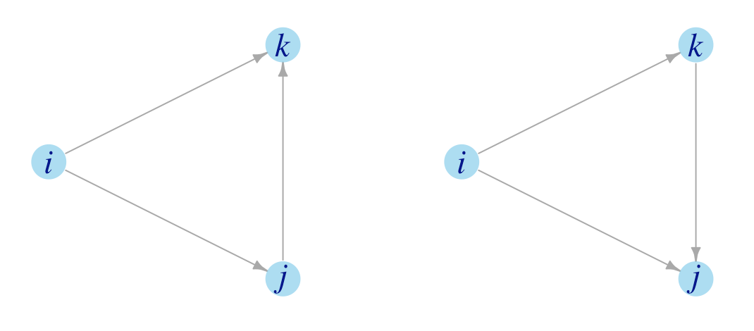
Figure 2: Transitive triangles

There are six potential transitive triangles that may exist within any triad; the figure above shows two of these (in which $i$ is the sender of two links). Additional links may exist within the triad and do not affect the existence of a transitive triangle.

In a dyadic link formation model in which $P(Y_{ij}=1|X,\phi)=F(\beta X_{ij}+\alpha_{i}+\gamma_{j})=p_{ij}$ say, the expected number of transitive triangles that will form is

$$T_{N}=\frac{1}{N(N-1)(N-2)}\sum_{i=1}^{N}\sum_{j\neq i}\sum_{k\neq\{i,j\}}p_{ij}p_{ik}p_{kj}.$$ (15)

This statistic is of the form 11, with $\lambda=\{(i,j),(i,k),(k,j)\}$ and $m_{\lambda}=p_{ij}p_{ik}p_{kj}$. Note that $m$ is not a function of the outcomes in this case, so the simpler leave-out estimate formula in 12 applies.

Specification testing

Another useful application of general fixed-effect averages is in specification testing. Dzemski (2019) proposed a test for the presence of strategic interactions in a model of link formation that is based on comparison of the observed number of transitive triangles to the expected number of triangles that would form in a dyadic model (i.e. 15). The test statistic is

$$T_{N}=\frac{1}{N(N-1)(N-2)}\sum_{i=1}^{N}\sum_{j\neq i}\sum_{k\neq\{i,j\}}\Big{(}Y_{ij}Y_{ik}Y_{kj}-p_{ij}p_{ik}p_{kj}\Big{)},$$

where $p_{ij}=\Phi(\beta X_{ij}+\alpha_{i}+\gamma_{j})$, for $\Phi$ the standard normal CDF. Here $Y_{ij}Y_{ik}Y_{kj}$ is an indicator for a transitive triangle and $p_{ij}p_{ik}p_{kj}$ is the probability of observing such a triangle under the conditional independence assumption in the dyadic model. Under the null hypothesis that the dyadic model is correct, the statistic is mean zero (when evaluated at $(\beta_{0},\phi_{0})$. In contrast, failure of the conditional independence assumption (Assumption 1 (i) in this paper), as would occur in the presence of strategic decision making by agents, will result in the statistic converging in probability to a non-zero limit. Dzemski (2019) derived an analytical bias correction for this statistic (and another based on cyclic triangles) for the case of a probit model. This statistic can also be jackknife bias-corrected as shown in this paper. In addition, the jackknife allows for specification tests like this to be extended to a range of other models, including models with non-binary outcomes, as well as a range of other statistics. For example, we could consider a range of test statistics based on the covariance between $(Y_{ij}-E[Y_{ij}|X,\phi])$ and some network statistic $S_{ij}$

$$T_{N}=\frac{1}{N(N-1)}\sum_{i}\sum_{j\neq i}(Y_{ij}-E[Y_{ij}|X,\phi])S_{ij}.$$ (16)

The choice of the statistic $S_{ij}$ may be motivated by the exact type of deviation from conditional independence the researcher is interested in testing. For example, $S_{ij}=Y_{ji}$ gives a test of reciprocity, i.e. the tendency of agents to be more likely to form a directed link if the corresponding link in the opposing direction already exists. Using $S_{ij}=\frac{1}{N-2}\sum_{k\neq\{i,j\}}Y_{ik}Y_{kj}$ gives a test for transitive triangles, similar to the one presented above. Graham and Pelican (2020) consider a similar set of test for a logit model, where sufficient statistics for the fixed effect parameters exist, and derive some optimal test statistics. It would seem useful to consider the properties of such test statistics in a broader set of models, although this is beyond the scope of this paper. We note only that many interesting statistics are likely to have the form of the general fixed effect averages considered in this paper, and so the jackknife bias correction may prove useful in forming such tests.

4.3 Asymptotic analysis for fixed effect averages

Here we present asymptotic results for the general fixed-effect averages. Recall that $\lambda$ is a set of observations $(i,j)$, and $\Lambda_{N}$ is the collection of all such sets formed by permuting the nodes in $\lambda$. We let $Y_{\lambda}=\{Y_{ij}\}_{(i,j)\in\lambda}$, $X_{\lambda}=\{X_{ij}\}_{(i,j)\in\lambda}$, and $\pi_{\lambda}=\{\alpha_{i}+\gamma_{j}\}_{(i,j)\in\lambda}$ collect the outcomes, covariates and fixed effects for the observations in $\lambda$. The function of interest is $m_{\lambda}=m(Y_{\lambda},X_{\lambda},\beta,\pi_{\lambda})$, which is a function of $(Y_{ij},X_{ij},\alpha_{i}+\gamma_{j})$ for each $(i,j)\in\lambda$.

We can decompose the difference between our jackknife estimate and the population average into three sources

$$\widehat{\Delta}_{J}-\delta=(\widehat{\Delta}_{J}-\Delta_{N})+(\Delta_{N}-\bar{\Delta}_{N})+(\bar{\Delta}_{N}-\delta).$$ (17)

The first term, $\widehat{\Delta}_{J}-\Delta_{N}$, represents variation caused by estimation of the parameters in the model, including fixed effects. The next term, $\Delta_{N}-\bar{\Delta}_{N}$, is variation of the sample outcomes $m_{\lambda}$ around their conditional expectations $\bar{m}_{\lambda}=E[m_{\lambda}|X,\phi]$. In the case that $m$ does not depend on outcomes $Y_{\lambda}$, we will have $m_{\lambda}=\bar{m}_{\lambda}$ and this second term will vanish. Finally, $\bar{\Delta}_{N}-\delta$ captures differences in the distribution of covariates and fixed effects in the observed network, relative to the population. In the case that the full network is observed, or whenever $\bar{\Delta}_{N}=0$, as is the case for specification tests discussed above, we will have that $\bar{\Delta}_{N}=\delta$.

In addition to Assumptions 1 and 2, we will impose regularity conditions on the choices of $\lambda$ and $m$.

Assumption 3 (Regularity conditions for fixed-effect averages).

Let $\lambda$ be a set of $r$ observations $(i,j)$ containing $p$ distinct agents. Let $\mathcal{B}_{\varepsilon}$ be a subset of $\mathbb{R}^{\dim\beta+r}$ that contains an $\varepsilon$-neighborhood of $(\beta{}_{0},\pi_{0,\lambda})$ for all $N$ and $\lambda$, with $\varepsilon>0$.

(i) Both $r$ and $p$ are fixed for all $N$. The set $\Lambda_{N}$ contains all $\frac{N!}{(N-p)!}$ permutations of $\lambda$.

(ii) The function $m$ depends on $(\alpha,\gamma)$ only through $\pi_{\lambda}=\{\alpha_{i}+\gamma_{j}\}_{(i,j)\in\lambda}$. For all $\lambda$, $m(Z_{\lambda},\beta,\pi_{\lambda})$ is five times continuously differentiable with respect to $\beta$ and $\pi_{\lambda}$ over $\mathcal{B}_{\varepsilon}$ a.s.; the partial derivatives of $m$ with respect to the elements of $(\beta,\pi_{\lambda})$ up to fifth order are bounded in absolute value uniformly over $(\beta,\pi_{\lambda})\in\mathcal{B}_{\varepsilon}$ by a function $M(Z_{\lambda})>0$ a.s.; and $\max_{\lambda}\bar{E}[M(Z_{\lambda})^{16}]$ is a.s. uniformly bounded over $N$.

(iii) We have that $0<\min_{\lambda}E[m_{\lambda}^{2}]-E[m_{\lambda}]^{2}\leq\max_{\lambda}E[m_{\lambda}^{2}]-E[m_{\lambda}]^{2}<\infty$ uniformly over $N$.

Assumption 3 (i) restricts $m$ to be a function of a fixed number of edges in the network, and assumes that $\Delta_{N}$ is an average of all possible arrangements of the nodes in $\lambda$. This ensures that sufficient averaging occurs over both dimensions of the fixed effects. For example, an average of the form $\frac{1}{N}\sum_{j\neq i}m(X_{ij},\alpha_{i},\gamma_{j})$ is not allowed since we are only averaging over the receiver dimension, while holding $i$ fixed.

Assumption 3 (ii) is analogous to Assumption 2 (ii), and imposes the same differentiability and moment conditions on $m$ as are imposed on $\ell$. This allows for asymptotic expansions of $\widehat{\Delta}_{N}$ to be derived, in the same way as for $\widehat{\beta}$. Finally, (iii) ensures that the unconditional second moments of $m$ are well defined.

Inference on the conditional average $\bar{\Delta}_{N}$

The asymptotic distribution of $\widehat{\Delta}_{J}$ depends on the choice of target parameter, either a conditional or population average. The following theorem states the asymptotic result for the jackknife bias-corrected estimator of the conditional fixed effect average $\bar{\Delta}_{N}$.

Theorem 2 (Jackknife estimator for fixed-effect averages).

Let Assumptions 1, 2 and 3 hold, and let $\widehat{\Delta}_{J}$ be the jackknife bias-corrected estimator in either (10) or (14). Then

$$N(\widehat{\Delta}_{J}-\bar{\Delta}_{N}) \Rightarrow\mathcal{N}(0,V_{\Delta}).$$

If we additionally assume that $E\big{[}(m_{\lambda}-\bar{m}_{\lambda})(m_{\lambda^{\prime}}-\bar{m}_{\lambda^{\prime}})\big{]}\neq 0$ for sets $\lambda$ and $\lambda^{\prime}$ that share exactly one observation in common, then the asymptotic variance is

$$V_{\Delta}=\lim_{N\to\infty}\frac{1}{N(N-1)}\sum_{i}\sum_{j<i}\bar{E}\big{[}(h_{ij}+s_{ij})^{2}\big{]}$$

where $h_{ij}=-N(\partial_{\theta}\bar{\Delta}_{N})(\partial_{\theta\theta^{\prime}}\bar{\mathcal{L}})^{-1}\big{(}(\partial_{\theta}\ell_{ij})+(\partial_{\theta}\ell_{ji})\big{)}$, for $\theta^{\prime}=(\beta,\alpha^{\prime},\gamma^{\prime})$, and $s_{ij}=\frac{(N-p)!}{(N-2)!}\sum_{\lambda\in\tilde{\Lambda}_{ij}}(m_{\lambda}-\bar{m}_{\lambda})$, with $\tilde{\Lambda}_{ij}=\{\lambda:(i,j)\in\lambda\text{ or }(j,i)\in\lambda\}$.

If we have either $m_{\lambda}=\bar{m}_{\lambda}$ or $E\big{[}(m_{\lambda}-\bar{m}_{\lambda})(m_{\lambda^{\prime}}-\bar{m}_{\lambda^{\prime}})\big{]}=0$ for sets $\lambda$ and $\lambda^{\prime}$ that share exactly one observation in common, then the asymptotic variance is

$$V_{\Delta}=\lim_{N\to\infty}\frac{1}{N(N-1)}\sum_{i}\sum_{j<i}\bar{E}\big{[}h_{ij}^{2}\big{]}.$$

In either case, let $\widehat{V}_{\Delta}$ be the plug-in estimator for $V_{\Delta}$ that replaces the unknown $\theta$ with estimates $\widehat{\theta}$. Then $\widehat{V}_{\Delta}\to V_{\Delta}$.

Some explanation for the form of the variance may be useful. The two terms $h_{ij}$ and $s_{ij}$ relate to the first two components of (17). The first component $\widehat{\Delta}_{J}-\Delta_{N}$ contains variation from estimation of the common parameters $\beta$ and fixed effects $\alpha,\gamma$. In the Appendix it is shown that this term can be approximated using the delta-method

$$N(\widehat{\Delta}_{J}-\Delta_{N}) =-N(\partial_{\theta}\bar{\Delta}_{N})(\partial_{\theta\theta^{\prime}}\bar{\mathcal{L}})^{-1}(\partial_{\theta}\ell_{ij})+o_{p}(1)$$

$$=\frac{1}{N-1}\sum_{i}\sum_{j\neq i}h_{ij}+o_{p}(1).$$

Note that, replacing the jackknife estimate $\widehat{\Delta}_{J}$ with the standard estimator $\widehat{\Delta}_{N}$ would result in additional terms appearing in the above first-order approximation, related to the incidental parameter bias. The second component is

$$N(\Delta_{N}-\bar{\Delta}_{N}) =\frac{N}{|\Lambda_{N}|}\sum_{\lambda}(m_{\lambda}-\bar{m}_{\lambda}).$$

The variance of this term depends on the conditional covariance between $m_{\lambda}$ and $m_{\lambda^{\prime}}$ for distinct sets $\lambda$ and $\lambda^{\prime}$. Note that if $\lambda$ and $\lambda^{\prime}$ share no dyads in common then they are conditionally independent. The variance of this term depends on the condition $E\big{[}(m_{\lambda}-\bar{m}_{\lambda})(m_{\lambda^{\prime}}-\bar{m}_{\lambda^{\prime}})\big{]}\neq 0$ for sets $\lambda$ and $\lambda^{\prime}$ share exactly one observation in common. Under this condition, the variance of $\sum_{\lambda}(m_{\lambda}-\bar{m}_{\lambda})$ is dominated by covariances between $m_{\lambda}$ and $m_{\lambda^{\prime}}$ for $\lambda$ and $\lambda^{\prime}$ that share exactly one dyad in common; although $\lambda$ with two or more common dyads also contribute to the variance, there are an order of magnitude fewer such combinations, and so these represent smaller order contributions that do not appear in the asymptotic variance. In settings where $E\big{[}(m_{\lambda}-\bar{m}_{\lambda})(m_{\lambda^{\prime}}-\bar{m}_{\lambda^{\prime}})\big{]}=0$ for $\lambda$ and $\lambda^{\prime}$ that share exactly one observation in common, $\Delta_{N}-\bar{\Delta}_{N}$ is a degenerate U-statistic and its variance is asymptotically of smaller order than the variance from parameter estimation, i.e. $\widehat{\Delta}_{J}-\Delta_{N}$, and so may be ignored.

Inference on the population average $\delta$

Theorem 2 shows how we may construct confidence sets for the parameter of interest $\bar{\Delta}_{N}$. When the object of interest is the unconditional average $\delta$, the convergence of the estimator will be dominated by variation from the third component in (17), $\bar{\Delta}_{N}-\delta$. To describe the statistic in this setting, it is useful to use its U-statistic representation. We will additionally assume that $X_{ij}=h(X_{i},X_{j})$. This condition appears in other work on dyadic models, for example in Graham (2017). When $X_{ij}$ measures the similarity (or difference) between $i$ and $j$ in some measure, we will commonly have $X_{ij}=d(X_{i}-X_{j})$, for $d$ some distance function. Alternatively, if $X_{ij}$ captures common membership in some group, we may have $X_{ij}=X_{i}X_{j}$ where $X_{i}$ is an indicator for $i$’s membership.

To give $\bar{\Delta}_{N}$ a U-statistic representation, we first sum together all $\bar{m}_{\lambda}$ which share the same set of agents. Since there are $p$ agents in each $\lambda$, this gives $p!$ different $\lambda$ that can be created from a given set of agents. We denote these sets of unordered agents by $\tau$. We have, for $\tilde{m}=\bar{m}-E[m]$

$$\bar{\Delta}_{N}-\delta =\frac{1}{N\cdots(N-p+1)}\sum_{\lambda}\tilde{m}_{\lambda}$$

$$=\frac{p!}{N\cdots(N-p+1)}\sum_{\tau}\Big{(}\frac{1}{p!}\sum_{\lambda\in\tau}\tilde{m}_{\lambda}\Big{)}$$

$$={N\choose p}^{-1}\sum_{\tau}u_{\tau},$$

where $u_{\tau}=\frac{1}{p!}\sum_{\lambda\in\tau}\tilde{m}_{\lambda}$. The term $u_{\tau}$ is a symmetric function of $\{\beta,X_{i},\alpha_{i},\gamma_{i}\}$ for $p$ agents $i$. Assuming that the $\{X_{i},\alpha_{i},\gamma_{i}\}$ are i.i.d. over agents, $\bar{\Delta}_{N}-\delta$ is a U-statistic of order $p$ and we may apply standard theory on such statistics to compute its asymptotic distribution.

Theorem 3 (Population average effects).

Let Assumptions 1, 2 and 3 hold. Additionally, assume that $X_{ij}=h(X_{i},X_{j})$ where $X_{i}$ is an observed agent-specific characteristic, and also that $(\alpha_{i},\gamma_{i},X_{i})$ is i.i.d. over $i$. Let $\Sigma_{1}=Cov\big{(}u_{\tau},u_{\tau^{\prime}}\big{)}$, for $\tau,\tau^{\prime}$ such that $\tau\cap\tau^{\prime}=\{i\}$. Then, for $V_{\delta}=p^{2}\Sigma_{1}$

$$\sqrt{N}(\widehat{\Delta}_{J}-\delta) \Rightarrow\mathcal{N}(0,V_{\delta}).$$

Additionally, the variance estimator $\widehat{V}_{\delta}$ in (18) is consistent, i.e. $\widehat{V}_{\delta}\to V_{\delta}$.

The convergence rate in Theorem 3 is slower than the rate in Theorem 2. While $m_{\lambda}$ and $m_{\lambda^{\prime}}$ are conditionally independent when $\lambda$ and $\lambda^{\prime}$ share no dyads in common, the two are unconditionally independent only when they share no agents in common. Since there are many more sets $\lambda$ that share a single agent $i$ than share a dyad $(i,j)$, the variance of $\bar{\Delta}_{N}-\delta$ is an order of magnitude larger than that of $\widehat{\Delta}_{N}-\Delta_{N}$, and so the convergence rate is slower.

Similarly to Theorem 2, the variance is dominated by covariances between sets $\lambda$ that share exactly one node in common. The term $\Sigma_{1}$ is the covariance between $u_{\tau}$ and $u_{\tau^{\prime}}$ when $\tau$ and $\tau^{\prime}$ share exactly one agent in common. A consistent estimator for this quantity is given by

$$\widehat{V}_{\delta}=\frac{1}{N}\sum_{i}\tilde{\mu}_{i}^{2},$$ (18)

$$\tilde{\mu}_{i}=\frac{(N-p)!}{(N-1)!}\sum_{\lambda:i\in\lambda}(\widehat{\bar{m}}_{\lambda}-\widehat{\mu}),\quad\widehat{\mu} =\frac{(N-p)!}{N!}\sum_{\lambda}\widehat{m}_{\lambda},$$

where $\tilde{\mu}_{i}$ is the average over all sets $\lambda$ containing agent $i$, $\widehat{\bar{m}}_{\lambda}$ is a plug-in estimator for $\bar{m}_{\lambda}$, and $\widehat{\mu}=\sum_{\lambda}\widehat{\bar{m}}_{\lambda}$ is the overall mean.

Since the rate of convergence in Theorem 3 is $N^{-1/2}$, there is in fact no asymptotic bias generated by the incidental parameters. The bias from the estimation of the fixed effects is of order $N^{-1}$, which is smaller than the variation in the sampled distribution of fixed effects around is population distribution. Nonetheless, the bias corrected steo is still recommended as it is likely to improve the finite sample properties of inference, in terms of correct centering of confidence sets, with little or no cost in terms of additional variance. In the panel data setting, Fernández-Val and Weidner (2016) report such improvements in simulations.

5 Empirical example

Following Jochmans (2018), we apply the jackknife procedure to two empirical settings. The first is a country-level trade network in which the outcome is a binary indicator for the presence of a trading relationship between 136 countries. The data are taken from Santos Silva and Tenreyro (2006), and additional details on their construction can be found in that paper. We use several covariates to capture homophily in trade relationships: log distance, the log of the distance between the capitals of the countries; border, an indicator of whether the countries share a common border; language, an indicator for whether the countries share a language; colonial, and indicator for whether either country had colonized the other at some point in history; and trade agreement, an indicator for the presence of a joint preferential trade agreement between the two countries. The network is dense, with around half of all potential trade links forming; however, there is significant heterogeneity in both in and out degree. For example, the 10th percentile of out degree is just 26 (i.e. 10 % of countries export to fewer than 33 other countries), while the 90th percentile is 133 (i.e. 10% of countries export to at least all but two other countries).

Table 1 presents the estimates of the model using a probit specification. The signs and magnitudes of the coefficients have been discussed in detail elsewhere and so here we focus on the effect of the bias correction. The magnitude of all but on of the coefficients (the exception being border) decrease after bias correction. In particular, the magnitude of the impact of geographic distance on trade and of the effect of trade agreements decrease by more than a standard deviation. This aligns with the findings in Jochmans (2018), who uses a conditional logit estimator to correct for the incidental parameters bias, although we note that the effect of bias correction is less significant here.

Table 1: Gravity model estimates

	Parameter estimates					Marginal effects
	MLE	Jack	SE	Bias/SE		MLE	Jack	SE	Bias/SE
log distance	-0.730	-0.694	0.027	1.316		-0.113	-0.111	0.005	0.410
language	0.320	0.296	0.051	-0.479		0.050	0.048	0.008	-0.275
colony	0.300	0.262	0.053	-0.714		0.047	0.042	0.008	-0.532
trade agree.	1.105	0.882	0.169	-1.324		0.176	0.146	0.027	-1.118

*Bias/SE is ratio of the difference in the Jackknife and MLE estimates to the standard error.

In addition to bias correction for the parameters of the model, the jackknife method allows bias correction of the marginal effects. For the log distance variable, I compute the marginal effect as the average of $\varphi(\beta^{\prime}X_{ij}+\alpha_{i}+\gamma_{j})\beta_{ldist}$, i.e. the average of the derivative of the fitted probabilities. For the binary variables I compute the average of the difference between the fitted probabilities setting that variable to one versus zero, $\Phi(\beta^{\prime}X^{(1)}_{ij}+\alpha_{i}+\gamma_{j})-\Phi(\beta^{\prime}X^{(0)}_{ij}+\alpha_{i}+\gamma_{j})$. The results are contained in the right panel of Table 1. In general, the magnitude of the incidental parameters bias appears smaller when considering marginal effects, rather than the coefficient estimates (the has been noted elsewhere, for example Fernández-Val 2009).

Finally, I also test for the presence of transitivity in two networks: the trade network described above, as well as for a professional network of attorneys from Lazega (2001). In this network the outcome is an indicator for friendship between 71 attorneys at law firm. The network is sparser than the trade one, with only 11 per cent of all friendships forming. I include covariates for whether the attorneys are of the same gender, professional status, or work in the same office, as well as measures of the difference in their ages and tenure. I compute transitivity test statistics based on (16) using $S_{ij}=\frac{1}{N-2}\sum_{k\neq\{i,j\}}Y_{ik}Y_{kj}$. Similarly to Dzemski (2019), I compute standard errors for the statistics using an analytical bootstrap procedure, since the plug-in estimator for the variance appears to poorly approximate the truth in simulations. The results of the transitivity tests are presented in Table 2.

In both networks, jackknife bias correction has a large and important impact on the size of the t-statistics. The more complicated averages effects that make up the test statistics appear to suffer from the incidental parameters bias to a much greater extent than the simple average effects. In the case of the trade network, the uncorrected test statistic would suggest a strong rejection of the null hypothesis of a dyadic network formation model. In contrast, the bias-corrected t-statistic is close to zero, and suggests that the dyadic model does a good job of capturing the observed transitivity in the trade network. For the professional network the statistic becomes larger after bias correction, so that we do reject the dyadic model. This aligns with common findings that social networks tend to exhibit high degrees of transitivity and clustering.

Table 2: Transitivity test statistics

	MLE	Jackknife
trade network	-10.37	-0.74
professional network	14.12	21.30

6 Simulations

Here I demonstrate the effectiveness of the jackknife in simulations. I repeat the simulation design of Dzemski (2019), which has also been used in a number of other network papers. The binary outcome $Y_{ij}$ is determined by

$$Y_{ij}=1\{\theta X_{ij}+\alpha_{i}+\gamma_{j}>\varepsilon_{ij}\}$$

where $\theta=1$ and $\varepsilon_{ij}\sim N(0,1)$. Individual $i$ is characterized by the binary scalar $X_{i}=1-2\times 1\{i\text{ is odd}\}$, and the homophily variable is given by $X_{ij}=X_{i}X_{j}$, i.e. it is one for pairs with the same sign and minus one for pairs with opposing signs. The fixed effects are given by an equally spaced sequence from $C_{N}^{l}$ to $C_{N}^{u}$. The value of $(C_{N}^{l},C_{N}^{u})$ is intended to control the sparsity of the network, and I consider four choices, shown in Table 3. In first setting, fixed effects range between $\pm\log\log N$, generating a dense network in which around half of all links are formed. Subsequent settings feature increasingly sparse networks in which some nodes remain well connected, while others make few links. In the sparsest setting only around 3 per cent of all links are formed and the networks feature large numbers of disconnected agents. When computing the estimators, I first remove these disconnected agents from the network, and consider estimation in the smaller connected network. This has no effect on the MLE, since these agents have no influence on the common parameter estimate, but is important for construction of the leaveout sets.

Table 3: Fixed effect distributions

$(C_{N}^{l},C_{N}^{u})$	Density	Connected	Min	1st quart.	Median	3rd quart.	Max
$(\pm\log\log N)$	0.50	50.0	8.6	16.9	24.1	31.7	40.3
$(-\log\log N,0)$	0.19	50.0	2.0	6.3	9.2	12.5	19.0
$(-\log^{1/2}N,0)$	0.12	49.5	0.1	2.4	5.0	8.4	15.1
$(-\log N,0)$	0.03	29.4	0.0	0.0	0.5	2.6	8.2

*Values are averages over 1000 simulations in a network of $N=50$ nodes. Connected counts the number of agents that have at least one link

Table 4 presents the results of the MLE, analytical bias-corrected estimate, and both the standard and weighted jackknife bias-corrected over 1000 simulations. As expected, the MLE is biased, with the size of the bias increasing in the sparsity of the network. In each case, the bias is around one standard deviation in size, resulting in substantial over-rejection. Focussing on the first three designs, the jackknife estimator removes almost all of the bias. The weighted jackknife shows even better performance and appears approximately unbiased. In each case, the jackknife estimators have smaller standard deviation than the MLE, and rejection rates are close to or below the nominal level of 5 per cent.

In the sparsest design the jackknife estimator does not appear to perform well, and shows similar bias to the MLE. The weighted jackknife performs better, and remains close to median unbiased, with small standard errors. However, inference is still poor in the sparsest design for all estimators. This is expected since the bias corrections all require dense network asymptotics. Overall, the simulation evidence is supportive of the good performance of the jackknife method for bias correction in all but very sparse network settings.

Table 4: Simulation results

	MLE	BC	J	WJ		MLE	BC	J	WJ
	$-\log(\log n),\log(\log n)$					$-\log(\log n),0$
Bias (mean)	0.064	0.002	-0.006	-0.002		0.074	0.007	-0.010	-0.001
Bias (median)	0.064	0.002	-0.006	-0.003		0.071	0.004	-0.013	-0.006
Std. dev.	0.043	0.039	0.039	0.039		0.059	0.054	0.051	0.053
5-95 percentile	0.138	0.126	0.123	0.123		0.190	0.173	0.162	0.171
Rejection (5%)	0.327	0.036	0.040	0.039		0.265	0.047	0.037	0.042
	$-(\log n)^{1/2},0$					$-\log n,0$
Bias (mean)	0.105	0.018	-0.039	0.002		0.568		-0.475	0.289
Bias (median)	0.097	0.010	-0.031	-0.009		0.264	-0.009	-0.303	0.090
Std. dev.	0.102	0.091	0.121	0.096		0.629		1.009	0.553
5-95 percentile	0.272	0.244	0.213	0.248		1.598	1.680	2.924	1.704
Rejection (5%)	0.257	0.053	0.042	0.052		0.288	0.163	0.484	0.265

*MLE is the maximum likelihood probit estimate, BC uses the bias correction from Dzemski (2019), J and WJ are the jackknife and weighted jackknife proposed in this paper. In the sparsest design the bias-corrected estimator resulted in a number of very large outlier estimates.

Finally, I compare the jackknife method suggested in this paper to previous suggestions. Specifically, Cruz-Gonzalez et al. (2017) suggest two jackknife bias corrections for network models of the type considered in this paper. The first bias correction is based on a split-sample approach. Divide the agents into two halves, $A_{1}$ and $A_{2}$. Define $\widehat{\beta}_{\alpha,\gamma/2}=\frac{1}{2}(\widehat{\beta}_{\alpha,\gamma\in A_{1}}+\widehat{\beta}_{\alpha,\gamma\in A_{2}})$, where $\widehat{\beta}_{\alpha,\gamma\in A_{1}}$ is the estimator that uses only observations in which the receiver is in the first set of agents $A_{1}$, and $\widehat{\beta}_{\alpha,\gamma\in A_{2}}$ uses only observations in which the receiver is in $A_{2}$. Similarly, define $\widehat{\beta}_{\alpha/2,\gamma}=\frac{1}{2}(\widehat{\beta}_{\alpha\in A_{1},\gamma}+\widehat{\beta}_{\alpha\in A_{2},\gamma})$ as the average of the two estimators that split the sample based on sending agents. A split-sample jackknife is given by

$$\widehat{\beta}_{ss}=3\widehat{\beta}_{N}-\widehat{\beta}_{\alpha/2,\gamma}-\widehat{\beta}_{\alpha,\gamma/2}.$$

The second bias correction is based on dropping all observations associated with a particular agent. Let $\widehat{\beta}_{(i)}$ be the estimate using only observations in the sub-network that excludes agent $i$. Cruz-Gonzalez et al. (2017) define the ‘double’ correction as

$$\widehat{\beta}_{d}=N\widehat{\beta}_{N}-(N-1)\frac{1}{N}\sum_{i}\widehat{\beta}_{(i)}.$$

The leave-one-agent-out style jackknife differs from $\widehat{\beta}_{J}$ in (5), in that is removes fixed effect parameters from the model in each leave-out estimate, while the construction of the $\mathcal{I}_{k}$ sets in this paper is designed to keep the distribution of fixed effects constant across all leave-out samples. This appears to be an important property for the jackknife to perform well in settings with substantial unobserved heterogeneity. Table 5 reports results from simulations of the same model discussed above for the standard and weighted jackknife estimators as well as the split-sample and double corrections suggested by Cruz-Gonzalez et al. (2017). As is clear from the results, although the split-sample and double corrections appear to work well in the densest network design, they perform less well in settings with more heterogeneity and sparser networks. In particular, the split-sample correction has much larger variance, and removes less bias than the leave-one-out style corrections (Hahn et al. (2023) derive higher-order bias and variance expressions that explain this phenomenon in the panel setting).

Table 5: Comparison of jackknife methods

	J	WJ	D	SS		J	WJ	D	SS
	$-\log(\log n),\log(\log n)$					$-\log(\log n),0$
Bias (mean)	-0.006	-0.002	-0.013	-0.017		-0.01	-0.001	-0.020	-0.045
Bias (median)	-0.006	-0.003	-0.011	-0.017		-0.013	-0.006	-0.021	-0.032
Std. dev.	0.039	0.039	0.039	0.042		0.051	0.053	0.049	0.101
5-95 percentile	0.123	0.123	0.125	0.137		0.162	0.171	0.158	0.227
Rejection (5%)	0.040	0.039	0.030	0.064		0.037	0.042	0.033	0.111
	$-(\log n)^{1/2},0$					$-\log n,0$
Bias (mean)	-0.039	0.002	-0.089	-0.236		-0.475	0.289	-1.248	-1.471
Bias (median)	-0.031	-0.009	-0.058	-0.109		-0.303	0.090	-1.264	-1.428
Std. dev.	0.102	0.096	0.202	0.299		1.009	0.553	1.545	1.408
5-95 percentile	0.213	0.248	0.219	0.889		2.924	1.704	4.967	4.741
Rejection (5%)	0.042	0.052	0.093	0.402		0.484	0.265	0.628	0.615

*J and WJ are the jackknife and weighted jackknife proposed in this paper, while D and SS are the ‘double’ and split-sample corrections defined in Cruz-Gonzalez et al. (2017).

7 Conclusion

This paper presents a new method for bias correcting nonlinear dyadic network models with fixed effects. I provide a novel formulation of the jackknife method that applies to networks with both sender and receiver fixed effects. The jackknife method provides an ‘off-the-shelf’ procedure for bias correction that is easy to apply, and applicable to a wide set of models. It allows for discrete multivalued and continuous outcome variables, and is able to obtain estimates of average effects and counterfactual outcomes. In simulations, I show that the jackknife performs well, even in relatively low density networks, and outperforms previous suggestions for jackknife procedures.

In addition, I show how the jackknife can be used to bias correct averages of functions that depend on multiple observations, including dyads, triads, and tetrads in the network. These averages can be used to produce a wide array of statistics, including tests for the presence of strategic interactions in the network, such as reciprocity or transitivity.

The jackknife procedure proposed in this paper could potentially also be applied to dyadic network models that include a time dimension, so long as the two-way fixed effect structure of this paper is maintained. For example, by defining the link-level objective function as

$$\ell(Y_{ij},X_{ij},\beta,\alpha_{i}+\gamma_{j})=\frac{1}{T}\sum_{t}\ell(Y_{ijt},X_{ijt},\beta,\alpha_{i}+\gamma_{j})$$

the jackknife procedure would work by dropping all observations from $(i,j)$ together. Sufficient conditions under which such a specification would satisfy the assumptions of this paper would be useful to investigate. The jackknife correction may also be useful in the interactive fixed effect model of Chen et al. (2021), and establishing validity in this setting would also be useful.

Appendix A Notation and norms

The notation in the appendices follows that in the main paper. That is, denote partial derivatives of the objective function using subscripts, so that $\partial_{\beta}\mathcal{L}(\beta,\phi)$ denotes $\partial\mathcal{L}(\beta,\phi)/\partial\beta$ and so on, where $\phi^{\prime}=(\alpha^{\prime},\gamma^{\prime})$. When functions are evaluated at $\beta_{0},\phi_{0}$ the dependence on these arguments is dropped. We also use $\ell_{ij}$ as shorthand for the function $\ell(Z_{ij},\cdot)$, with $Z_{ij}=(Y_{ij},X_{ij})$. Let

$$\mathcal{S}(\beta,\phi)=\partial_{\phi}\mathcal{L}(\beta,\phi),\quad\quad\mathcal{S}_{\beta}(\beta,\phi)=\partial_{\beta}\mathcal{L}(\beta,\phi)$$

be the first derivatives of the objective function. We also write $\mathcal{H}(\beta,\phi)=-\partial_{\phi\phi^{\prime}}\mathcal{L}(\beta,\phi)$ for the negative of the Hessian with respect to the fixed effects, a $2N\times 2N$ matrix.

We follow Fernandez-Val and Weidner (2016) (FVW) in using the Euclidean norm $\lVert\cdot\rVert$ for $\dim\beta$ vectors, and the norm induced by the Euclidean norm for matrices and tensors, i.e.

$$\lVert\partial_{\beta\beta\beta}\mathcal{L}(\beta,\phi)\rVert=\max_{u,v\in\mathbb{R}^{\dim\beta}:\lVert u\rVert=1,\lVert v\rVert=1}\lVert\sum_{k,l=1}^{\dim\beta}u_{k}v_{l}\partial_{\beta\beta_{k}\beta_{l}}\mathcal{L}(\beta,\phi)\rVert$$

In the proofs we sometimes take $\beta$ to be a scalar to simplify notation, although the results apply to any vector of fixed size. Since the number of fixed effect parameters in the model grows with $N$, the choice of norm for $\dim\phi$ vectors and matrices is important. Following FVW, we choose the $\ell_{q}$-norm for $\dim\phi$ vectors and the corresponding induced norms for matrices and tensors

$$\lVert\partial_{\phi\phi\phi}\mathcal{L}(\beta,\phi)\rVert=\max_{u,v\in\mathbb{R}^{\dim\phi}:\lVert u\rVert=1,\lVert v\rVert=1}\lVert\sum_{k,l=1}^{\dim\beta}u_{k}v_{l}\partial_{\phi\phi_{k}\phi_{l}}\mathcal{L}(\beta,\phi)\rVert_{q}$$

See FVW for more details on these norms. We define the sets $\mathcal{B}(r,\beta_{0})=\{\beta:\lVert\beta-\beta_{0}\rVert\leq r\}$, for $r>0$, and $\mathcal{B}_{q}(r,\phi_{0})=\{\phi:\lVert\phi-\phi_{0}\rVert_{q}\leq r\}$.

Appendix B Asymptotic expansions

The results in the paper are based on asymptotic expansions of the objective function. Fernández-Val and Weidner (2016) (FVW) derive expansions for a general class of M-estimators with multiple incidental parameters, which includes the model studied here. In the Supplementary Appendix I show that the expansions in that paper are applicable to the dyadic model considered in this paper (this follows Dzemski (2019) who verifies the FVW conditions for a dyadic probit model). In order to determine the properties of the jackknife estimator, I also extend the expansions in FVW to higher-order, which requires additional conditions on the number of moments and derivatives of the objective function that exist. Derivations of higher-order terms and their bounds are quite long and largely similar to the derivations in FVW, and so are provided in the Supplementary Appendix. This appendix contains analysis based on the first-order expansions and focuses on results related to the jackknife, which are of most interest.

The next lemma gives the asymptotic expansion for the estimated fixed effects and common parameters. It is largely a restatement of Theorem B.1 in Fernández-Val and Weidner (2016), but the remainder terms are split into two parts. The expressions for the remainder terms are given in the Supplementary Appendix, and are used to derive the properties of the jackknife bias correction. The proof of Lemma 4 is provided in the Supplementary Appendix.

Lemma 4.

Let Assumptions 1 and 2 hold. Then,

$$\widehat{\phi}-\phi_{0} =\mathcal{H}^{-1}\mathcal{S}+\frac{1}{N}\mathcal{H}^{-1}(\partial_{\phi\beta^{\prime}}\mathcal{L})\bar{W}_{N}^{-1}\big{(}U^{(0)}+U^{(1)}\big{)}$$

$$+\frac{1}{2}\mathcal{H}^{-1}\sum_{g=1}^{\dim\phi}(\partial_{\phi\phi^{\prime}\phi_{g}}\mathcal{L})\mathcal{H}^{-1}\mathcal{S}[\mathcal{H}^{-1}\mathcal{S}]_{g}$$

$$+R_{\phi}+\tilde{R}_{\phi}$$

and

$$N\bar{W}_{N}(\widehat{\beta}-\beta_{0})=U^{(0)}+U^{(1)}+R_{\beta}+\tilde{R}_{\beta}$$

where

$$U^{(0)} =(\partial_{\beta}\mathcal{L})+(\partial_{\beta\phi^{\prime}}\bar{\mathcal{L}})\bar{\mathcal{H}}^{-1}\mathcal{S}$$

$$U^{(1)} =(\partial_{\beta\phi^{\prime}}\tilde{\mathcal{L}})\bar{\mathcal{H}}^{-1}\mathcal{S}-(\partial_{\beta\phi^{\prime}}\bar{\mathcal{L}})\bar{\mathcal{H}}^{-1}\tilde{\mathcal{H}}\bar{\mathcal{H}}^{-1}\mathcal{S}$$

$$+\frac{1}{2}\sum_{g=1}^{\dim\phi}\big{(}(\partial_{\beta\phi\phi_{g}}\bar{\mathcal{L}})+(\partial_{\beta\phi^{\prime}}\bar{\mathcal{L}})\bar{\mathcal{H}}^{-1}(\partial_{\phi\phi^{\prime}\phi_{g}}\bar{\mathcal{L}})\big{)}\big{[}\bar{\mathcal{H}}^{-1}\mathcal{S}\big{]}_{g}\bar{\mathcal{H}}^{-1}\mathcal{S}$$

and the remainders satisfy $\lVert R_{\phi}\rVert=o_{p}(1)$, $\lVert R_{\beta}\rVert=o_{p}(1)$ and $\lVert\tilde{R}_{\phi}\rVert=o_{p}(N^{-1})$, $\lVert\tilde{R}_{\beta}\rVert=o_{p}(N^{-1})$.

We next state an important result on the approximation of the inverse of the Hessian for the fixed effect parameters. Let $\bar{\mathcal{H}}=\bar{E}[\mathcal{H}]$, $\tilde{\mathcal{H}}=\mathcal{H}-\bar{\mathcal{H}}$, and similarly for other conditional expectations and their residuals. As in FVW, we may write

$$\bar{\mathcal{H}}=\begin{bmatrix}\bar{\mathcal{H}}_{\alpha\alpha}^{*}&\bar{\mathcal{H}}_{\alpha\gamma}^{*}\\ \bar{\mathcal{H}}_{\gamma\alpha}^{*}&\bar{\mathcal{H}}_{\gamma\gamma}^{*}\end{bmatrix}+\frac{1}{N}bv_{N}v_{N}^{\prime}$$

where $\bar{\mathcal{H}}_{\alpha\alpha}^{*}$ and $\bar{\mathcal{H}}_{\gamma\gamma}^{*}$ are the diagonal matrices with elements

$$\big{(}\bar{\mathcal{H}}_{\alpha\alpha}^{*}\big{)}_{ii} =-\frac{1}{N-1}\sum_{j\neq i}\bar{E}[\partial_{\pi^{2}}\ell_{ij}]$$

$$\big{(}\bar{\mathcal{H}}_{\gamma\gamma}^{*}\big{)}_{ii} =-\frac{1}{N-1}\sum_{j\neq i}\bar{E}[\partial_{\pi^{2}}\ell_{ji}]$$

and $\bar{\mathcal{H}}_{\alpha\gamma}^{*}=(\bar{\mathcal{H}}_{\gamma\alpha}^{*})^{\prime}$ has off-diagonal entries $\big{(}\bar{\mathcal{H}}_{\alpha\gamma}^{*}\big{)}_{ij}=-\bar{E}[\partial_{\pi^{2}}\ell_{ij}]/(N-1)$ and zeroes in diagonal entries. We can show that $\bar{\mathcal{H}}^{-1}$ is dominated by its diagonal elements.

Lemma 5.

Let Assumptions 1 and 2 hold. Then,

$$\lVert\bar{\mathcal{H}}^{-1}-diag\big{(}\bar{\mathcal{H}}_{\alpha\alpha}^{*},\bar{\mathcal{H}}_{\gamma\gamma}^{*}\big{)}^{-1}\rVert_{max} =O_{p}(N^{-1})$$

Proof.

The proof is essentially identical to that of Lemma D.1 in Fernández-Val and Weidner (2016) or Lemma A.1 in Dzemski (2019) ∎

Appendix C Jackknife results for $\beta$

Here we allow for a more general construction of the leave-out sets, but impose two important conditions.

Condition 1.

Let $\mathcal{I}_{k}$ for $k=1,\dots N_{k}$ be a partition of the observations in a network of size $N$. Define $1_{ij}^{k}=1\{(i,j)\not\in\mathcal{I}_{k}\}$ as an indicator that the observation $(i,j)$ is not included in the $k$-th set. We impose the following conditions on the sets:

(i) $\sum_{k=1}^{N_{k}}(1-1_{ij}^{k})=1$ for all $(i,j)$

(ii) $\sum_{j\neq i}(1-1_{ij}^{k})=\sum_{i\neq j}(1-1_{ij}^{k})=l$ for all $i$, $j$, and $k$, for some fixed $l$.

Condition 1 imposes two important constrains on the sets $\mathcal{I}_{k}$: (i) that they are mutually exclusive, such that every edge $(i,j)$ appears in exactly one of the sets, and (ii) that each set contains exactly one observation related to each of the $N$ sender fixed effects $\alpha$ and each of the $N$ receiver fixed effects $\gamma$. The first condition ensures that all observations are used equally in the jackknife, and is important for showing that the asymptotic variance of the estimator is not affected by the jackknife. The second condition ensures that each fixed effect parameter is affected equally in the leave-out sets, and that $\bar{\mathcal{H}}_{(k)}$ is well-defined and positive definite. We assume in the proofs below that $l=1$, i.e. that we are using the leave-one-out jackknife as this simplifies notation. All of the results still hold for the leave-$l$-out style jackknife for fixed $l$.

Some additional notation will also be useful for studying the jackknife estimates. Let $A$ be some statistic and $A_{(k)}$ the same statistic in the $k$-th leave-out sample. We define the jackknife operator $\mathbf{J}$ as

$$\mathbf{J}[A]=A_{J}=(N-1)A-(N-2)\frac{1}{N-1}\sum_{k=1}^{N-1}A_{(k)}$$

Additionally, we define a set of indicators that count the number of unique leave-out sets $\mathcal{I}_{k}$ that a group of edges $(i_{1},j_{1}),\dots,(i_{t},j_{t})$ are contained in. Let

$$I_{(i_{1},j_{1}),\dots,(i_{t},j_{t})}^{r}=\begin{cases}1&(i_{1},j_{1}),\dots,(i_{t},j_{t})\text{ span exactly $r$ of the sets }\mathcal{I}_{k}\\ 0&\text{otherwise}\end{cases}$$

We begin by stating an expansion for the leave-out estimates $\widehat{\beta}_{(k)}$ and $\widehat{\phi}_{(k)}$. To do so, we apply the same set of expansions as in 4, but redefine the objective function to include indicator variables for the dropped observations. Let $\ell^{(k)}(Y_{ij},X_{ij}^{(k)},\beta,\alpha_{i}+\gamma_{j})=\ell(Y_{ij},X_{ij},\beta,\alpha_{i}+\gamma_{j})1_{ij}^{k}\frac{N-1}{N-2}$, where $X_{ij}^{(k)}=(X_{ij},1_{ij}^{k})$, so that we have

$$\mathcal{L}_{N,(k)}=\frac{1}{N-1}\sum_{i}\sum_{j\neq i}\ell_{ij}^{(k)}-\frac{b}{2N}\big{(}\sum_{i}\alpha_{i}-\sum_{i}\gamma_{i}\big{)}^{2}$$ (19)

Note that the new objective function satisfies the conditions of Assumptions 1 and 2 whenever $\ell_{ij}$ does, and we have independence of $\ell_{ij}^{(k)}$ (and its derivatives) from $\ell_{st}^{(k)}$ (and its derivatives), conditional on $X^{(k)},\phi$ for all $(i,j)\neq(s,t),(t,s)$ as required for the expansions. In order to derive the leave-out expansion, we first show leave-out versions of matrix sums can be approximated using the full-sample conditional expectations. Note that, since we are now conditioning on the leave-out sample indicators $1_{ij}^{k}$, the expansion for the leave-out estimators would include terms like $\bar{\mathcal{H}}_{(k)}^{-1}$ rather than the full-sample terms $\bar{\mathcal{H}}^{-1}$. The next lemma shows that the full sample matrix expectations provide a good approximation to the leave-out matrices, so that the full sample expectation may be used in the asymptotic expansion.

Lemma 6.

Let Assumptions 1 and 2 hold. Let $M$ be a matrix of the form

$$M=\begin{bmatrix}M_{\alpha\alpha}&M_{\alpha\gamma}\\ M_{\gamma\alpha}&M_{\gamma\gamma}\end{bmatrix}$$

where $M_{\alpha\alpha}$ and $M_{\gamma\gamma}$ are diagonal matrices with elements

$$(M_{\alpha\alpha})_{ii}=\frac{1}{N-1}\sum_{j\neq i}A_{ij},\quad(M_{\gamma\gamma})_{ii}=\frac{1}{N-1}\sum_{j\neq i}A_{ji}$$

and $M_{\alpha\gamma}=M_{\gamma\alpha}$ has zero diagonals and non-diagonal elements $\frac{1}{N-1}A_{ij}$, where $\max_{i,j}E[|A_{ij}|^{16}]\leq C$. Let $M_{(k)}$ be the equivalent matrix in the leave-out sample, and let $\bar{M}=\bar{E}[M]$. Then,

$$\lVert M-\bar{M}\rVert =O_{p}(N^{-7/16})$$

$$\lVert M_{(k)}-\bar{M}\rVert =O_{p}(N^{-7/16})$$

Proof.

To show the first result, note that

$$\bar{E}\lVert M_{\alpha\alpha}-\bar{M}_{\alpha\alpha}\rVert^{16} =\bar{E}\Big{[}\max_{i}\big{(}\frac{1}{N-1}\sum_{j\neq i}\partial_{\pi^{2}}\tilde{A}_{ij}\big{)}^{16}\Big{]}$$

$$\leq\sum_{i}\bar{E}\Big{[}\big{(}\frac{1}{N-1}\sum_{j\neq i}\partial_{\pi^{2}}\tilde{A}_{ij}\big{)}^{16}\Big{]}$$

$$\leq C\frac{1}{(N-1)^{8}}\sum_{i}\bar{E}\big{[}|\partial_{\pi^{2}}\tilde{A}_{ij}|^{16}\big{]}$$

$$=O_{p}(N^{-7})$$

since the observations in the sum are conditionally independent and $\max_{i,j}E[|\partial_{\pi^{2}}\tilde{A}_{ij}|^{16}]\leq C$ by assumption. This implies $\lVert M_{\alpha\alpha}-\bar{M}_{\alpha\alpha}\rVert=O_{p}(N^{-7/16})$. The same result applies for $M_{\gamma\gamma}$ using identical reasoning. For the final term, we can apply Lemma S.6 in FW16, noting that we have conditional independence in both dimensions, and that we may use $q=16$ in place of $q=8$ (with straightforward adjustments to the proof). This then gives $\lVert M-\bar{M}\rVert=O_{p}(N^{-7/16})$.

To show the same bound holds for the leave-out matrix, note that we have

$$(M_{(k),\alpha\alpha})_{ii}-(\bar{M}_{\alpha\alpha})_{ii} =\frac{1}{N-1}\sum_{j\neq i}\big{(}\partial_{\pi^{2}}A_{ij}1_{ij}^{k}\frac{N-1}{N-2}-\partial_{\pi^{2}}\bar{A}_{ij}\big{)}$$

$$=\frac{1}{N-2}\sum_{j\neq i}\big{(}\partial_{\pi^{2}}A_{ij}-\partial_{\pi^{2}}\bar{A}_{ij}\big{)}1_{ij}^{k}$$

$$+\frac{1}{N-1}\sum_{j\neq i}(\partial_{\pi^{2}}\bar{A}_{ij})\big{(}1_{ij}^{k}\frac{N-1}{N-2}-1\big{)}$$

$$=\frac{1}{N-2}\sum_{j\neq i}(\partial_{\pi^{2}}\tilde{A}_{ij})1_{ij}^{k}$$

$$+\frac{1}{(N-1)(N-2)}\sum_{j\neq\{i,i^{*}\}}(\partial_{\pi^{2}}\bar{A}_{ij})-\frac{1}{N-1}(\partial_{\pi^{2}}\bar{A}_{ii^{*}})$$

where $i^{*}$ is the receiver such that $(i,i^{*})\in\mathcal{I}_{k}$. The first term can be bounded identically to before. For the second term

$$\bar{E}\Big{[}\max_{i}\big{(}\frac{1}{(N-1)(N-2)}\sum_{j\neq\{i,i^{*}\}}(\partial_{\pi^{2}}\bar{A}_{ij})\big{)}^{16}\Big{]}\leq O(N^{-32})\sum_{i}\bar{E}\Big{[}\big{(}\sum_{j\neq i}\partial_{\pi^{2}}\bar{A}_{ij}\big{)}^{16}\Big{]}\leq O(N^{-15})$$

and similarly for the final term. Application of the triangle inequality gives $\lVert M_{(k),\alpha\alpha}-\bar{M}_{\alpha\alpha}\rVert=O_{p}(N^{-7/16})$. Identical reasoning applies to the other components of $M_{(k)}$, giving the result. ∎

We can now state the asymptotic expansion for the leave-out estimators. The proof is contained in the Supplementary Appendix, but is analogous to the full-sample version. We use the subscript $(k)$ to denote derivatives of the leave-out objective function (19), and $\partial_{\beta\phi^{\prime}}\bar{\mathcal{L}}_{(k)}=E[\partial_{\beta\phi^{\prime}}\mathcal{L}_{(k)}|X^{(k)},\phi]$ etc.

Lemma 7.

Let Assumptions 1 and 2 hold. Then,

$$N\bar{W}_{N}(\widehat{\beta}_{(k)}-\beta_{0})=U_{(k)}^{(0)}+U_{(k)}^{(1)}+R_{\beta,(k)}+\tilde{R}_{\beta,(k)}$$

where

$$U_{(k)}^{(0)} =(\partial_{\beta}\mathcal{L}_{(k)})+(\partial_{\beta\phi^{\prime}}\bar{\mathcal{L}})\bar{\mathcal{H}}^{-1}\mathcal{S}_{(k)}$$

$$U_{(k)}^{(1)} =(\partial_{\beta\phi^{\prime}}\tilde{\mathcal{L}}_{(k)})\bar{\mathcal{H}}^{-1}\mathcal{S}_{(k)}-(\partial_{\beta\phi^{\prime}}\bar{\mathcal{L}})\bar{\mathcal{H}}^{-1}\tilde{\mathcal{H}}_{(k)}\bar{\mathcal{H}}^{-1}\mathcal{S}_{(k)}$$

$$+\frac{1}{2}\sum_{g=1}^{\dim\phi}\big{(}(\partial_{\beta\phi\phi_{g}}\bar{\mathcal{L}})+(\partial_{\beta\phi^{\prime}}\bar{\mathcal{L}})\bar{\mathcal{H}}^{-1}(\partial_{\phi\phi^{\prime}\phi_{g}}\bar{\mathcal{L}})\big{)}\big{[}\bar{\mathcal{H}}^{-1}\mathcal{S}_{(k)}\big{]}_{g}\bar{\mathcal{H}}^{-1}\mathcal{S}_{(k)}$$

and the remainders satisfy $\lVert R_{\beta,(k)}\rVert=o_{p}(1)$ and $\lVert\tilde{R}_{\beta,(k)}\rVert=o_{p}(N^{-1})$, and similarly for the expansion of $\widehat{\phi}_{(k)}$, with $\lVert R_{\phi,(k)}\rVert=o_{p}(1)$ and $\lVert\tilde{R}_{\phi,(k)}\rVert=o_{p}(N^{-1})$.

C.1 Jackknifing first-order expansion terms

We next use this result to show the impact of the jackknife operator on the first-order expansion of $N(\widehat{\beta}-\beta)$. From the expansion in Lemma 4, we have that a first-order approximation is given by

$$N\bar{W}_{N}(\widehat{\beta}-\beta) =\big{(}U^{(0)}+U^{(1)}\big{)}+o_{p}(1)$$

The next lemmas demonstrate the effect of the jackknife on general sums of the forms in $U^{(0)}$ and $U^{(1)}$.

Lemma 8.

Let $1_{ij}^{k}$ satisfy Condition 1. For $A_{ij}$ a mean-zero random variable, let

$$A_{i} =\frac{1}{N-1}\sum_{s\neq i}A_{is},\qquad A_{(k),i}=\frac{1}{N-2}\sum_{s\neq i}A_{is}1_{is}^{k}$$

Define the jackknifed version of $A_{J,i}=\mathbf{J}[A_{i}]=(N-1)A_{i}-(N-2)\frac{1}{N-1}\sum_{k=1}^{N-1}A_{i}^{k}$. Then, $A_{J,i}=A_{i}$.

Proof.

First note that by Condition 1, $\sum_{k}1_{is}^{k}=N-2$. Then, $\sum_{k}A_{(k),i}=\sum_{s\neq i}A_{is}$ so that

$$A_{J,i} =(N-1)A_{i}-(N-2)\frac{1}{N-1}\sum_{k=1}^{N-1}A_{(k),i}$$

$$=(N-1)A_{i}-(N-2)\frac{1}{N-1}\sum_{s\neq i}A_{is}$$

$$=\frac{1}{N-1}\sum_{s\neq i}A_{is}=A_{i}$$

∎

Lemma 9.

Let $1_{ij}^{k}$ satisfy Condition 1. For $A_{ij}$ a mean-zero random variable with bounded fourth moment, let

$$\mathbf{A} =\frac{1}{N-1}\big{(}\{\sum_{s\neq i}A_{is}\}_{i=1,\dots,N},\{\sum_{s\neq j}A_{sj}\}_{j=1,\dots,N}\big{)}$$

$$=(\mathbf{A}_{\alpha},\mathbf{A}_{\gamma})$$

$$\mathbf{A}_{k} =\frac{1}{N-2}\big{(}\{\sum_{s\neq i}A_{is}1_{is}^{k}\}_{i=1,\dots,N},\{\sum_{s\neq j}A_{sj}1_{sj}^{k}\}_{j=1,\dots,N}\big{)}$$

$$=(\mathbf{A}_{\alpha,k},\mathbf{A}_{\gamma,k})$$

and let $\mathbf{B}$ and $\mathbf{B}_{k}$ be similarly defined vectors of sums involving mean-zero random variables $B_{ij}$. Assume that $(A_{ij},B_{ij})$ are independent of $(A_{st},B_{st})$ for $(i,j)\not\in\{(s,t),(t,s)\}$. Define the jackknifed term

$$\mathcal{J}_{0}= (N-1)\mathbf{A}^{\prime}M\mathbf{B}-\frac{N-2}{N-1}\sum_{k}\mathbf{A}_{(k)}^{\prime}M\mathbf{B}_{(k)}$$

where $M$ is a non-random matrix that has $O_{p}(1)$ elements on its diagonal and $O_{p}(N^{-1})$ off-diagonal terms. Then we have $\mathcal{J}_{0}=o_{p}(1)$.

Proof.

The most common choice of $M$ will be $\bar{\mathcal{H}}^{-1}$, which satisfies the conditions for $M$ by Assumptions 1 and 2 and the approximation property in (LABEL:eq:H_approx). We show the proof using $\bar{\mathcal{H}}^{-1}$, but note that it holds for any $M$ satisfying the conditions stated above. We have

$$\mathbf{A}^{\prime}\bar{\mathcal{H}}^{-1}\mathbf{B} =\mathbf{A}_{\alpha}^{\prime}\bar{\mathcal{H}}_{\alpha\alpha}^{-1}\mathbf{B}_{\alpha}+\mathbf{A}_{\alpha}^{\prime}\bar{\mathcal{H}}_{\alpha\gamma}^{-1}\mathbf{B}_{\gamma}$$

$$+\mathbf{A}_{\gamma}^{\prime}\bar{\mathcal{H}}_{\gamma\alpha}^{-1}\mathbf{B}_{\alpha}+\mathbf{A}_{\gamma}^{\prime}\bar{\mathcal{H}}_{\gamma\gamma}^{-1}\mathbf{B}_{\gamma}$$

Recall that $I_{(ij)(st)}^{1}$ is one whenever $(i,j)$ and $(s,t)$ are contained in the same $\mathcal{I}_{k}$, and so $\sum_{k}1_{ij}^{k}1_{st}^{k}=(N-2)I_{(ij)(st)}^{1}+(N-3)(1-I_{(ij)(st)}^{1})$.

$$\mathbf{A}_{\alpha}^{\prime}\bar{\mathcal{H}}_{\alpha\alpha}^{-1}\mathbf{B}_{\alpha} =\sum_{i,j}\mathbf{A}_{\alpha,i}(\bar{\mathcal{H}}_{\alpha\alpha}^{-1})_{ij}\mathbf{B}_{\alpha,j}$$

$$=\frac{1}{(N-1)^{2}}\sum_{i,j}\sum_{s\neq i}\sum_{t\neq j}(\bar{\mathcal{H}}_{\alpha\alpha}^{-1})_{ij}A_{is}B_{jt}$$

$$\frac{1}{N-1}\sum_{k}\mathbf{A}_{k,\alpha}^{\prime}\bar{\mathcal{H}}_{\alpha\alpha}^{-1}\mathbf{B}_{k,\alpha} =\frac{1}{(N-1)(N-2)^{2}}\sum_{k}\sum_{i,j}\sum_{s\neq i}\sum_{t\neq j}(\bar{\mathcal{H}}_{\alpha\alpha}^{-1})_{ij}A_{is}B_{jt}1_{is}^{k}1_{jt}^{k}$$

$$=\frac{1}{(N-1)(N-2)}\sum_{i,j}\sum_{s\neq i}\sum_{t\neq j}(\bar{\mathcal{H}}_{\alpha\alpha}^{-1})_{ij}A_{is}B_{jt}I_{(is)(jt)}^{1}$$

$$+\frac{N-3}{(N-1)(N-2)^{2}}\sum_{i,j}\sum_{s\neq i}\sum_{t\neq j}(\bar{\mathcal{H}}_{\alpha\alpha}^{-1})_{ij}A_{is}B_{jt}(1-I_{(is)(jt)}^{1})$$

Then, we have

$$\mathcal{J}_{\alpha\alpha}= (N-1)\mathbf{A}_{\alpha}^{\prime}\bar{\mathcal{H}}_{\alpha\alpha^{\prime}}^{-1}\mathbf{B}_{\alpha}-\frac{N-2}{N-1}\sum_{k}\mathbf{A}_{\alpha,k}^{\prime}\bar{\mathcal{H}}_{\alpha\alpha^{\prime}}^{-1}\mathbf{B}_{\alpha,k}$$

$$= \frac{1}{(N-1)(N-2)}\sum_{i}\sum_{j}\sum_{s\neq i}\sum_{t\neq j}(\bar{\mathcal{H}}_{\alpha\alpha^{\prime}}^{-1})_{ij}\big{(}A_{is}B_{jt}\big{)}(1-I_{(is)(jt)}^{1})$$

Similar computations for the other three elements gives

$$\mathcal{J}_{0}= (N-1)\mathbf{A}^{\prime}\bar{\mathcal{H}}^{-1}\mathbf{B}-\frac{N-2}{N-1}\sum_{k}\mathbf{A}_{k}^{\prime}\bar{\mathcal{H}}^{-1}\mathbf{B}_{k}$$

$$= \frac{1}{(N-1)(N-2)}\sum_{i}\sum_{j}\sum_{s\neq i}\sum_{t\neq j}\Big{\{}(\bar{\mathcal{H}}_{\alpha\alpha^{\prime}}^{-1})_{ij}+(\bar{\mathcal{H}}_{\alpha\gamma^{\prime}}^{-1})_{it}$$

$$+(\bar{\mathcal{H}}_{\gamma\alpha^{\prime}}^{-1})_{sj}+(\bar{\mathcal{H}}_{\gamma\gamma^{\prime}}^{-1})_{st}\Big{\}}\big{(}A_{is}B_{jt}\big{)}(1-I_{(is)(jt)}^{1})$$

Let $\Gamma_{ijst}=(\bar{\mathcal{H}}_{\alpha\alpha^{\prime}}^{-1})_{ij}+(\bar{\mathcal{H}}_{\alpha\gamma^{\prime}}^{-1})_{it}+(\bar{\mathcal{H}}_{\gamma\alpha^{\prime}}^{-1})_{sj}+(\bar{\mathcal{H}}_{\gamma\gamma^{\prime}}^{-1})_{st}$. We have

$$\Gamma_{ijst}=\begin{cases}O_{p}(1)&i=j\text{ or }s=t\\ O_{p}(N^{-1})&\text{otherwise}\end{cases}$$

We can decompose $\mathcal{J}_{0}$ as

$$\mathcal{J}_{0} =\frac{1}{(N-1)(N-2)}\sum_{i}\sum_{j}\Big{(}\sum_{s<i}\sum_{t<j}\Gamma_{ijst}A_{is}B_{jt}+\sum_{s<i}\sum_{t>j}\Gamma_{ijst}A_{is}B_{jt}$$

$$+\sum_{s>i}\sum_{t<j}\Gamma_{ijst}A_{is}B_{jt}+\sum_{s>i}\sum_{t>j}\Gamma_{ijst}A_{is}B_{jt}\Big{)}(1-I_{(is)(jt)}^{1})$$

$$=\mathcal{J}_{0,11}+\mathcal{J}_{0,12}+\mathcal{J}_{0,21}+\mathcal{J}_{0,22}$$

Then we have

$$\bar{E}[\mathcal{J}_{0,11}^{2}] =\frac{1}{(N-1)^{2}(N-2)^{2}}\sum_{i}\sum_{j}\sum_{k}\sum_{l}\sum_{s<i}\sum_{t<j}\sum_{p<k}\sum_{q<l}\Gamma_{ijst}\Gamma_{klpq}$$

$$\times E\big{[}A_{is}B_{jt}A_{kp}B_{lq}\big{]}(1-I_{(is)(jt)}^{1})(1-I_{(kp)(lq)}^{1})$$

$$=\frac{1}{(N-1)^{2}(N-2)^{2}}\sum_{i}\sum_{j}\sum_{s<i}\sum_{t<j}\Gamma_{ijst}^{2}\bar{E}[A_{is}^{2}B_{jt}^{2}](1-I_{(is)(jt)}^{1})$$

$$+\frac{2}{(N-1)^{2}(N-2)^{2}}\sum_{i}\sum_{j}\sum_{s<i}\sum_{t<j}\Gamma_{ijst}\Gamma_{stij}\bar{E}[A_{is}B_{is}A_{jt}B_{jt}\big{]}(1-I_{(is)(jt)}^{1})$$

$$=\frac{1}{(N-1)^{2}(N-2)^{2}}\sum_{i}\sum_{s<i}\sum_{t<i}\Gamma_{iist}^{2}\bar{E}[A_{is}^{2}B_{it}^{2}](1-I_{(is)(it)}^{1})$$

$$+\frac{1}{(N-1)^{2}(N-2)^{2}}\sum_{i}\sum_{j\neq i}\sum_{s<(i\wedge j)}\Gamma_{ijss}^{2}\bar{E}[A_{is}^{2}]\bar{E}[B_{js}^{2}](1-I_{(is)(js)}^{1})$$

$$+\frac{1}{N^{2}(N-1)^{2}(N-2)^{2}}\sum_{i}\sum_{j\neq i}\sum_{s<i}\sum_{t<j,t\neq s}N^{2}\Gamma_{ijst}^{2}\bar{E}[A_{is}^{2}]\bar{E}[B_{jt}^{2}](1-I_{(is)(jt)}^{1})$$

$$+\frac{2}{(N-1)^{2}(N-2)^{2}}\sum_{i}\sum_{s<i}\sum_{t<i}\Gamma_{iist}\Gamma_{stii}\bar{E}[A_{is}B_{is}]\bar{E}[A_{it}B_{it}\big{]}(1-I_{(is)(it)}^{1})$$

$$+\frac{2}{(N-1)^{2}(N-2)^{2}}\sum_{i}\sum_{j\neq i}\sum_{s\neq(i\wedge j)}\Gamma_{ijss}\Gamma_{ssij}\bar{E}[A_{is}B_{is}]\bar{E}[A_{js}B_{js}\big{]}(1-I_{(is)(js)}^{1})$$

$$+\frac{1}{N^{2}(N-1)^{2}(N-2)^{2}}\sum_{i}\sum_{j\neq i}\sum_{s<i}\sum_{t<j,t\neq s}N^{2}\Gamma_{ijst}\Gamma_{stij}\bar{E}[A_{is}B_{is}]\bar{E}[A_{jt}B_{jt}\big{]}(1-I_{(is)(jt)}^{1})$$

$$=O_{p}(N^{-1})$$

Where the last line follows from the properties of $\Gamma_{ijst}$. The same result holds for $\bar{E}[\mathcal{J}_{0,12}^{2}]$, $\bar{E}[\mathcal{J}_{0,21}^{2}]$, and $\bar{E}[\mathcal{J}_{0,22}^{2}]$, hence $\mathcal{J}_{0}=O_{p}(N^{-1/2})=o_{p}(1)$. ∎

The following lemma derives the forms of $\mathbf{J}[U^{(0)}]$ and $\mathbf{J}[U^{(1)}]$.

Lemma 10.

Let Assumptions 1 and 2 hold. Then

$$\mathbf{J}[U^{(0)}] =U^{(0)}$$

$$\mathbf{J}[U^{(1)}] =o_{p}(1)$$

Proof.

For $U^{(0)}=(\partial_{\beta}\mathcal{L})+(\partial_{\beta\phi^{\prime}}\bar{\mathcal{L}})\bar{\mathcal{H}}^{-1}\mathcal{S}$ we can appeal to Lemma 8 with $A_{i}=(\partial_{\beta}\mathcal{L})_{i}=\frac{1}{N-1}\sum_{j\neq i}\partial_{\beta}\ell_{ij}$ and with $A_{i}=\mathcal{S}_{i}=\frac{1}{N-1}\sum_{j\neq i}\partial_{\pi}\ell_{ij}$. Note that the jackknife operator is linear so that, since $(\partial_{\beta\phi^{\prime}}\bar{\mathcal{L}})\bar{\mathcal{H}}^{-1}$ are fixed across leave-out samples,

$$\mathbf{J}[\partial_{\beta}\mathcal{L}] =\sum_{i}\mathbf{J}[(\partial_{\beta}\mathcal{L})_{i}]$$

$$\mathbf{J}\big{[}(\partial_{\beta\phi^{\prime}}\bar{\mathcal{L}})\bar{\mathcal{H}}^{-1}\mathcal{S}\big{]} =(\partial_{\beta\phi^{\prime}}\bar{\mathcal{L}})\bar{\mathcal{H}}^{-1}\mathbf{J}[\mathcal{S}]$$

Now, for $U^{(1)}$ we can appeal to Lemma 9. For the first term, $(\partial_{\beta\phi^{\prime}}\tilde{\mathcal{L}})\bar{\mathcal{H}}^{-1}\mathcal{S}$ we set $A_{ij}=\partial_{\beta\pi}\tilde{\ell}_{ij}$ and $B_{ij}=\partial_{\pi}\ell_{ij}$. For the second term, $(\partial_{\beta\phi^{\prime}}\bar{\mathcal{L}})\bar{\mathcal{H}}^{-1}\tilde{\mathcal{H}}\bar{\mathcal{H}}^{-1}\mathcal{S}$ we note that

$$(\partial_{\beta\phi^{\prime}}\bar{\mathcal{L}})\bar{\mathcal{H}}^{-1}\tilde{\mathcal{H}}=\big{(}(\partial_{\beta\phi^{\prime}}\bar{\mathcal{L}})\bar{\mathcal{H}}^{-1}\tilde{\mathcal{H}}_{\cdot,\alpha},(\partial_{\beta\phi^{\prime}}\bar{\mathcal{L}})\bar{\mathcal{H}}^{-1}\tilde{\mathcal{H}}_{\cdot,\gamma}\big{)}$$

where the $i$-th element of $(\partial_{\beta\phi^{\prime}}\bar{\mathcal{L}})\bar{\mathcal{H}}^{-1}\tilde{\mathcal{H}}_{\cdot,\alpha}$ is

$$(\partial_{\beta\phi^{\prime}}\bar{\mathcal{L}})\bar{\mathcal{H}}^{-1}\tilde{\mathcal{H}}_{\cdot,\alpha_{i}} =(\partial_{\beta\alpha^{\prime}}\bar{\mathcal{L}})\bar{\mathcal{H}}_{\alpha\alpha}^{-1}\tilde{\mathcal{H}}_{\alpha\alpha_{i}}+(\partial_{\beta\alpha^{\prime}}\bar{\mathcal{L}})\bar{\mathcal{H}}_{\alpha\gamma}^{-1}\tilde{\mathcal{H}}_{\gamma\alpha_{i}}$$

$$+(\partial_{\beta\gamma^{\prime}}\bar{\mathcal{L}})\bar{\mathcal{H}}_{\gamma\alpha}^{-1}\tilde{\mathcal{H}}_{\alpha\alpha_{i}}+(\partial_{\beta\gamma^{\prime}}\bar{\mathcal{L}})\bar{\mathcal{H}}_{\gamma\gamma}^{-1}\tilde{\mathcal{H}}_{\gamma\alpha_{i}}$$

$$=-(\partial_{\beta\alpha^{\prime}}\bar{\mathcal{L}})\bar{\mathcal{H}}_{\alpha\alpha_{i}}^{-1}\frac{1}{N-1}\sum_{j\neq i}\partial_{\pi^{2}}\tilde{\ell}_{ij}-\frac{1}{N-1}\sum_{j\neq i}(\partial_{\beta\alpha^{\prime}}\bar{\mathcal{L}})\bar{\mathcal{H}}_{\alpha\gamma_{j}}^{-1}\partial_{\pi^{2}}\tilde{\ell}_{ij}$$

$$-(\partial_{\beta\gamma^{\prime}}\bar{\mathcal{L}})\bar{\mathcal{H}}_{\gamma\alpha_{i}}^{-1}\frac{1}{N-1}\sum_{j\neq i}\partial_{\pi^{2}}\tilde{\ell}_{ij}-\frac{1}{N-1}\sum_{j\neq i}(\partial_{\beta\gamma^{\prime}}\bar{\mathcal{L}})\bar{\mathcal{H}}_{\gamma\gamma_{j}}^{-1}\partial_{\pi^{2}}\tilde{\ell}_{ij}$$

and similarly for elements of $(\partial_{\beta\phi^{\prime}}\bar{\mathcal{L}})\bar{\mathcal{H}}^{-1}\tilde{\mathcal{H}}_{\cdot,\gamma}$. So we can let

$$A_{ij}=\big{(}(\partial_{\beta\alpha^{\prime}}\bar{\mathcal{L}})\bar{\mathcal{H}}_{\alpha\alpha_{i}}^{-1}+(\partial_{\beta\alpha^{\prime}}\bar{\mathcal{L}})\bar{\mathcal{H}}_{\alpha\gamma_{j}}^{-1}+(\partial_{\beta\gamma^{\prime}}\bar{\mathcal{L}})\bar{\mathcal{H}}_{\gamma\alpha_{i}}^{-1}+(\partial_{\beta\gamma^{\prime}}\bar{\mathcal{L}})\bar{\mathcal{H}}_{\gamma\gamma_{j}}^{-1}\big{)}\partial_{\pi^{2}}\tilde{\ell}_{ij}$$

and $B_{ij}=\partial_{\pi}\ell_{ij}$ in Lemma 9. Note that we have $A_{ij}$ and $B_{ij}$ mean zero and the moment condition also holds by assumption. For the final term, we begin by demonstrating that both $\bar{\mathcal{H}}^{-1}\sum_{g}(\partial_{\beta\phi^{\prime}\phi_{g}}\bar{\mathcal{L}})\bar{\mathcal{H}}^{-1}$and $\bar{\mathcal{H}}^{-1}\sum_{g}(\partial_{\phi\phi^{\prime}\phi_{g}}\bar{\mathcal{L}})\big{[}\bar{\mathcal{H}}^{-1}(\partial_{\beta\phi}\bar{\mathcal{L}})\big{]}_{g}\bar{\mathcal{H}}^{-1}$are matrices that satisfy the requirements for $M$ in Lemma 9. The proof for the second term is shown, with the result for the first term following nearly identically. Firstly,

$$\sum_{g} (\partial_{\phi\phi^{\prime}\phi_{g}}\bar{\mathcal{L}})\big{[}\bar{\mathcal{H}}^{-1}(\partial_{\beta\phi}\bar{\mathcal{L}})\big{]}_{g}$$

$$=\sum_{s,t}(\partial_{\phi\phi^{\prime}\alpha_{s}}\bar{\mathcal{L}})\big{(}\bar{\mathcal{H}}_{\alpha\alpha}^{-1}\big{)}_{st}(\partial_{\beta\alpha_{t}}\bar{\mathcal{L}})+\sum_{s,t}(\partial_{\phi\phi^{\prime}\gamma_{s}}\bar{\mathcal{L}})\big{(}\bar{\mathcal{H}}_{\gamma\alpha}^{-1}\big{)}_{st}(\partial_{\beta\alpha_{t}}\bar{\mathcal{L}})$$

$$+\sum_{s,t}(\partial_{\phi\phi^{\prime}\alpha_{s}}\bar{\mathcal{L}})\big{(}\bar{\mathcal{H}}_{\alpha\gamma}^{-1}\big{)}_{st}(\partial_{\beta\gamma_{t}}\bar{\mathcal{L}})+\sum_{s,t}(\partial_{\phi\phi^{\prime}\gamma_{s}}\bar{\mathcal{L}})\big{(}\bar{\mathcal{H}}_{\gamma\gamma}^{-1}\big{)}_{st}(\partial_{\beta\gamma_{t}}\bar{\mathcal{L}})$$

Taking the first of these terms, the $(i,j)$ element is given by

$$\big{[}\sum_{s,t} (\partial_{\phi\phi^{\prime}\alpha_{s}}\bar{\mathcal{L}})\big{(}\bar{\mathcal{H}}_{\alpha\alpha}^{-1}\big{)}_{st}(\partial_{\beta\alpha_{t}}\bar{\mathcal{L}})\big{]}_{ij}$$

$$=\sum_{t}(\partial_{\phi_{i}\phi_{j}^{\prime}\alpha_{t}}\bar{\mathcal{L}})\big{(}\bar{\mathcal{H}}_{\alpha\alpha}^{-1}\big{)}_{tt}(\partial_{\beta\alpha_{t}}\bar{\mathcal{L}})+\frac{1}{N}\sum_{t}\sum_{s\neq t}(\partial_{\phi_{i}\phi_{j}^{\prime}\alpha_{s}}\bar{\mathcal{L}})\big{(}N\bar{\mathcal{H}}_{\alpha\alpha}^{-1}\big{)}_{st}(\partial_{\beta\alpha_{t}}\bar{\mathcal{L}})$$

Now if $\phi_{i}=\phi_{j}=\alpha_{i}$ then

$$\sum_{t}(\partial_{\phi_{i}\phi_{j}^{\prime}\alpha_{t}}\bar{\mathcal{L}})\big{(}\bar{\mathcal{H}}_{\alpha\alpha}^{-1}\big{)}_{tt}(\partial_{\beta\alpha_{t}}\bar{\mathcal{L}})=(\partial_{\alpha_{i}^{3}}\bar{\mathcal{L}})\big{(}\bar{\mathcal{H}}_{\alpha\alpha}^{-1}\big{)}_{ii}(\partial_{\beta\alpha_{i}}\bar{\mathcal{L}})=O_{p}(1)$$

and if $\phi_{i}=\phi_{j}=\gamma_{i}$ then

$$\sum_{t}(\partial_{\phi_{i}\phi_{j}^{\prime}\alpha_{t}}\bar{\mathcal{L}})\big{(}\bar{\mathcal{H}}_{\alpha\alpha}^{-1}\big{)}_{tt}(\partial_{\beta\alpha_{t}}\bar{\mathcal{L}})=\frac{1}{N-1}\sum_{t\neq i}(\partial_{\alpha_{t}\gamma_{i}^{2}}\bar{\mathcal{\ell}}_{ti})\big{(}\bar{\mathcal{H}}_{\alpha\alpha}^{-1}\big{)}_{tt}(\partial_{\beta\alpha_{t}}\bar{\mathcal{L}})=O_{p}(1)$$

Finally, if $i\neq j$ then we have either 0, or

$$\sum_{t}(\partial_{\phi_{i}\phi_{j}^{\prime}\alpha_{t}}\bar{\mathcal{L}})\big{(}\bar{\mathcal{H}}_{\alpha\alpha}^{-1}\big{)}_{tt}(\partial_{\beta\alpha_{t}}\bar{\mathcal{L}})=\frac{1}{N-1}(\partial_{\pi\alpha_{t}\gamma_{i}}\bar{\mathcal{\ell}}_{ti})\big{(}\bar{\mathcal{H}}_{\alpha\alpha}^{-1}\big{)}_{tt}(\partial_{\beta\alpha_{t}}\bar{\mathcal{L}})=O_{p}(N^{-1})$$

Identical results apply to the other elements in $\sum_{g}(\partial_{\phi\phi^{\prime}\phi_{g}}\bar{\mathcal{L}})\big{[}\bar{\mathcal{H}}^{-1}(\partial_{\beta\phi}\bar{\mathcal{L}})\big{]}_{g}$ and hence we can conclude that the matrix has $O_{p}(1)$ diagonal elements and $O_{p}(N^{-1})$ off-diagonal elements. It then follows that the same is true of $\bar{\mathcal{H}}^{-1}\sum_{g}(\partial_{\phi\phi^{\prime}\phi_{g}}\bar{\mathcal{L}})\big{[}\bar{\mathcal{H}}^{-1}(\partial_{\beta\phi}\bar{\mathcal{L}})\big{]}_{g}\bar{\mathcal{H}}^{-1}$. Then, we can apply Lemma 9 with $\mathbf{A}=\mathbf{B}=\mathcal{S}$ to give the result. ∎

Lemma 11.

Let Assumptions 1 and 2 hold, and let $\widehat{\beta}_{J}$ be the either the jackknife estimator. Then, a first-order approximation to the estimator is given by

$$\bar{W}_{N}N(\widehat{\beta}_{J}-\beta_{0})=U^{(0)}+o_{p}(1)$$

where $U^{(0)}=(\partial_{\beta}\mathcal{L})+(\partial_{\beta\phi^{\prime}}\bar{\mathcal{L}})\bar{\mathcal{H}}^{-1}\mathcal{S}$.

Proof.

Recall from Lemma 4 that

$$N\bar{W}_{N}(\widehat{\beta}-\beta_{0})=U^{(0)}+U^{(1)}+R_{\beta}+\tilde{R}_{\beta}$$

Since $\bar{W}_{N}$ is fixed across leave-out samples, we can focus on the jackknife operator applied to the RHS. By Lemma 10 we have that $\mathbf{J}[U^{(0)}+U^{(1)}]=U^{(0)}+o_{p}(1)$, while in the Supplementary Appendix it is shown that $\mathbf{J}[R_{\beta}]=o_{p}(1)$. Finally,

$$\mathbf{J}[\tilde{R}_{\beta}] =(N-1)\tilde{R}_{\beta}-(N-2)\frac{1}{N-1}\sum_{k}\tilde{R}_{\beta,(k)}$$

$$=o_{p}(1)$$

since each remainder term in the above is $o_{p}(N^{-1})$. ∎

C.2 Proof of Theorem 1

From Lemma 11 we have that

$$\bar{W}_{N}N(\widehat{\beta}_{J}-\beta_{0}) =(\partial_{\beta}\mathcal{L})+(\partial_{\beta\phi^{\prime}}\bar{\mathcal{L}})\bar{\mathcal{H}}^{-1}\mathcal{S}+o_{p}(1)$$

$$=\frac{1}{N-1}\sum_{i}\sum_{j<i}\big{(}D_{\beta}\ell_{ij}+D_{\beta}\ell_{ji}\big{)}$$

where $D_{\beta}\ell_{ij}=\partial_{\beta}\ell_{ij}-\partial_{\pi}\ell_{ij}\Xi_{ij}$ for

$$\Xi_{ij} =-\frac{1}{N-1}\sum_{s}\sum_{t\neq s}\Gamma_{ijst}\bar{E}[\partial_{\beta\pi}\ell_{st}]$$

$$\Gamma_{ijst} =(\bar{\mathcal{H}}_{\alpha\alpha}^{-1})_{is}+(\bar{\mathcal{H}}_{\gamma\alpha}^{-1})_{js}+(\bar{\mathcal{H}}_{\alpha\gamma}^{-1})_{it}+(\bar{\mathcal{H}}_{\gamma\gamma}^{-1})_{jt}$$

The result then follows from a standard CLT argument. To show consistency of the plug-in estimator $\widehat{\Omega}_{N}$, we note that by Assumption 2 (iii), $D_{\beta}\ell_{ij}$ has a first-order Taylor approximation that is a continuously differentiable function of the parameters. Then by the continuous mapping theorem and the consistency of parameter estimates $\lVert\widehat{\beta}-\beta_{0}\rVert\to 0$ and $\lVert\widehat{\phi}-\phi\rVert_{\infty}\to 0$ (see Theorem B.3. in FVW), $\widehat{\Omega}_{N}\to\Omega$ as required (see for example Lemma S.1 in FVW).

Appendix D Jackknife results for average effects

We begin by stating a first-order asymptotic expansion for the average effect estimator that will be used in the proof of Theorem 2. The proof of this result is provided in the Supplementary Appendix.

Lemma 12.

Let Assumptions 1, 2 and 3 hold. Then

$$N(\widehat{\Delta}_{N}-\Delta_{N}) =\Big{[}(\partial_{\beta}\bar{\Delta}_{N})-(\partial_{\phi^{\prime}}\bar{\Delta}_{N})\mathcal{\bar{H}}^{-1}(\partial_{\beta\phi}\bar{\mathcal{L}})\Big{]}\bar{W}_{N}^{-1}\big{(}U^{(0)}+U^{(1)}\big{)}$$

$$+N(\partial_{\phi^{\prime}}\bar{\Delta}_{N})\mathcal{\bar{H}}^{-1}\mathcal{S}$$

$$+N(\partial_{\phi^{\prime}}\tilde{\Delta}_{N})\mathcal{\bar{H}}^{-1}\mathcal{S}-N(\partial_{\phi^{\prime}}\bar{\Delta}_{N})\mathcal{\bar{H}}^{-1}\mathcal{\tilde{H}}\mathcal{\bar{H}}^{-1}\mathcal{S}$$

$$+\frac{1}{2}N\mathcal{S}^{\prime}\bar{\mathcal{H}}^{-1}\Big{(}(\partial_{\phi\phi^{\prime}}\bar{\Delta}_{N})+\sum_{g}(\partial_{\phi\phi^{\prime}\phi_{g}}\bar{\mathcal{L}})[(\partial_{\phi^{\prime}}\bar{\Delta}_{N})\mathcal{\bar{H}}^{-1}]_{g}\Big{)}\mathcal{\bar{H}}^{-1}\mathcal{S}$$

$$+R_{\Delta}+\tilde{R}_{\Delta}$$

where $\lVert R_{\Delta}\rVert=o_{p}(1)$, and $\lVert\tilde{R}_{\Delta}\rVert=o_{p}(N^{-1})$, and

$$N(\widehat{\Delta}_{(k)}-\Delta_{N}) =\Big{[}(\partial_{\beta}\bar{\Delta}_{N})-(\partial_{\phi^{\prime}}\bar{\Delta}_{N})\mathcal{\bar{H}}^{-1}(\partial_{\beta\phi}\bar{\mathcal{L}})\Big{]}\bar{W}_{N}^{-1}\big{(}U_{(k)}^{(0)}+U_{(k)}^{(1)}\big{)}$$

$$+N(\partial_{\phi^{\prime}}\bar{\Delta}_{N})\mathcal{\bar{H}}^{-1}\mathcal{S}_{(k)}$$

$$+N(\partial_{\phi^{\prime}}\tilde{\Delta}_{(k)})\mathcal{\bar{H}}^{-1}\mathcal{S}_{(k)}-N(\partial_{\phi^{\prime}}\bar{\Delta}_{N})\mathcal{\bar{H}}^{-1}\mathcal{\tilde{H}}_{(k)}\mathcal{\bar{H}}^{-1}\mathcal{S}_{(k)}$$

$$+\frac{1}{2}N\mathcal{S}_{(k)}^{\prime}\bar{\mathcal{H}}^{-1}\Big{(}(\partial_{\phi\phi^{\prime}}\bar{\Delta}_{N})+\sum_{g}(\partial_{\phi\phi^{\prime}\phi_{g}}\bar{\mathcal{L}})[(\partial_{\phi^{\prime}}\bar{\Delta}_{N})\mathcal{\bar{H}}^{-1}]_{g}\Big{)}\mathcal{\bar{H}}^{-1}\mathcal{S}_{(k)}$$

$$+R_{(k),\Delta}+\tilde{R}_{(k),\Delta}$$

where $\lVert R_{(k),\Delta}\rVert=o_{p}(1)$, and $\lVert\tilde{R}_{(k),\Delta}\rVert=o_{p}(N^{-1})$.

The next lemmas are used to bound the jackknifed versions of the new forms of product terms appearing in the expansion for the average effects.

Lemma 13.

Let $\lambda$ be a set of $r$ observations $(i,j)$ involving $p$ unique agents, and $\Lambda_{N}$ be the collection of all such $\lambda$ formed by permuting the agents in $\lambda$. Then, under Assumption 3,

(i) $\partial_{\phi}\bar{\Delta}_{N}$ has $O_{p}(N^{-1})$ elements

(ii) $\partial_{\alpha\alpha^{\prime}}\bar{\Delta}_{N}$, $\partial_{\alpha\gamma^{\prime}}\bar{\Delta}_{N}$, $\partial_{\gamma\alpha^{\prime}}\bar{\Delta}_{N}$, and $\partial_{\gamma\gamma^{\prime}}\bar{\Delta}_{N}$ each have $O_{p}(N^{-1})$ diagonal elements and $O_{p}(N^{-2})$ off-diagonal elements

Proof.

Let $\lambda_{\alpha}$ denote the set of $p_{\alpha}$ sender agents in the observations within $\lambda$, and $\lambda_{\gamma}$ the set of $p_{\gamma}$ receiving agents. There are $|\Lambda_{N}|=\frac{N!}{(N-p)!}$ ways of selecting the $p$ agents in $\lambda$. Among these permutations, agent $i$ is a sender $p_{\alpha}\frac{(N-1)!}{(N-p)!}$ times, while node $j$ is the receiver $p_{\gamma}\frac{(N-1)!}{(N-p)!}$ times. Using this, the first derivatives of $\bar{\Delta}_{N}$ with respect to the fixed effects are

$$\partial_{\alpha_{i}}\bar{\Delta}_{N} =\frac{1}{|\Lambda_{N}|}\sum_{\lambda:i\in\lambda_{\alpha}}\partial_{\alpha_{i}}\bar{m}_{\lambda}=O_{p}(N^{-1})$$

$$\partial_{\gamma_{i}}\bar{\Delta}_{N} =\frac{1}{|\Lambda_{N}|}\sum_{\lambda:i\in\lambda_{\gamma}}\partial_{\gamma_{i}}\bar{m}_{\lambda}=O_{p}(N^{-1})$$

where the $O_{p}(N^{-1})$ statements come from the fact that $p_{\alpha}\frac{(N-1)!}{(N-p)!}/\frac{N!}{(N-p)!}=p_{\alpha}/N$. An identical result applies to the diagonal elements of $\partial_{\phi\phi^{\prime}}\bar{\Delta}_{N}$, i.e. $\partial_{\alpha_{i}\alpha_{i}}\bar{\Delta}_{N}=O_{p}(N^{-1})$ and $\partial_{\gamma_{j}\gamma_{j}}\bar{\Delta}_{N}=O_{p}(N^{-1})$ since they are sums over the same sets of $\lambda$. Also, if the presence of $i$ as a sender agent implies that $i$ is also a receiver in $\lambda$ (e.g. the cyclic triangle $\{(i,j),(j,k),(k,i)\}$) then it will be the case that $\partial_{\alpha_{i}\gamma_{i}}\bar{\Delta}_{N}=O_{p}(N^{-1})$ also (if this is not true it will be lower order).

Next, consider the off-diagonal components of $\partial_{\phi\phi^{\prime}}\bar{\Delta}_{N}$. If $p_{\alpha}=1$ then $\partial_{\alpha_{i}\alpha_{j}}\bar{\Delta}_{N}=0$, otherwise, there are ${p_{\alpha}\choose 2}\frac{(N-2)!}{(N-p)!}$ permutations that contain both $i$ and $j$ as senders. Similarly, for $p_{\gamma}\geq 2$, there are ${p_{\gamma}\choose 2}\frac{(N-2)!}{(N-p)!}$ permutations that contain both $i$ and $j$ as receivers. Finally, there are at most $p_{\alpha}p_{\gamma}\frac{(N-2)!}{(N-p)!}$ permutations in which $i$ is a sender and $j$ a receiver (this is an upper bound since with $i$ in a particular sender position, not all receiver positions may be valid for $j$). This, along with Assumption 3, gives the results

$$\partial_{\alpha_{i}\alpha_{j}}\bar{\Delta}_{N} =O_{p}(N^{-2})$$

$$\partial_{\alpha_{i}\gamma_{j}}\bar{\Delta}_{N} =O_{p}(N^{-2})$$

$$\partial_{\gamma_{i}\gamma_{j}}\bar{\Delta}_{N} =O_{p}(N^{-2})$$

which demonstrates the lemma. ∎

Lemma 14.

Let $1_{ij}^{k}$ satisfy Condition 1 and let $1_{\lambda}^{k}=\prod_{(i,j)\in\lambda}1_{ij}^{k}$ and define $\Lambda_{is}=\{\lambda:(i,s)\in\lambda\}$, i.e. the set of all $\lambda$ containing observation $(i,s)$. Let $A_{ij}$ be a mean-zero random variable with bounded fourth moment, and define

$$\mathbf{A} =\frac{1}{N-1}\big{(}\{\sum_{s\neq i}A_{is}\}_{i=1,\dots,N},\{\sum_{s\neq j}A_{sj}\}_{j=1,\dots,N}\big{)}$$

$$=(\mathbf{A}_{\alpha},\mathbf{A}_{\gamma})$$

$$\mathbf{A}_{k} =\frac{1}{N-2}\big{(}\{\sum_{s\neq i}A_{is}1_{is}^{k}\}_{i=1,\dots,N},\{\sum_{s\neq j}A_{sj}1_{sj}^{k}\}_{j=1,\dots,N}\big{)}$$

$$=(\mathbf{A}_{\alpha,k},\mathbf{A}_{\gamma,k})$$

and let $\mathbf{B}$ and $\mathbf{B}_{k}$ be defined as

$$\mathbf{B} =\frac{N}{|\Lambda_{N}|}\big{(}\{\sum_{s\neq i}\sum_{\lambda\in\Lambda_{is}}B_{\lambda}\}_{i=1,\dots,N},\{\sum_{s\neq j}\sum_{\lambda\in\Lambda_{sj}}B_{\lambda}\}_{i=1,\dots,N}\big{)}$$

$$=(\mathbf{B}_{\alpha},\mathbf{B}_{\gamma})$$

$$\mathbf{B}_{k} =\frac{N-1}{N-r-1}\frac{N}{|\Lambda_{N}|}\big{(}\{\sum_{s\neq i}\sum_{\lambda\in\Lambda_{is}}B_{\lambda}1_{\lambda}^{k}\}_{i=1,\dots,N},\{\sum_{s\neq j}\sum_{\lambda\in\Lambda_{sj}}B_{\lambda}1_{\lambda}^{k}\}_{i=1,\dots,N}\big{)}$$

$$=(\mathbf{B}_{\alpha,k},\mathbf{B}_{\gamma,k})$$

for mean zero $B_{\lambda}$ with bounded fourth moment. Assume that $A_{ij}$ is independent of $A_{st}$ for $(i,j)\not\in\{(s,t),(t,s)\}$, and independent of $B_{\lambda}$ whenever $\lambda$ does not contain either $(i,j)$ or $(j,i)$. Define the jackknifed term

$$\mathcal{J}_{0}= (N-1)\mathbf{A}^{\prime}M\mathbf{B}-\frac{N-2}{N-1}\sum_{k}\mathbf{A}_{(k)}^{\prime}M\mathbf{B}_{(k)}$$

where $M$ is a non-random matrix that has $O_{p}(1)$ elements on its diagonal and $O_{p}(N^{-1})$ off-diagonal terms. Then we have $\mathcal{J}_{0}=o_{p}(1)$.

Proof.

The most common choice of $M$ will be $\bar{\mathcal{H}}^{-1}$, which satisfies the conditions for $M$ by Assumptions 1 and 2 and (LABEL:eq:H_approx). We show the proof using $\bar{\mathcal{H}}^{-1}$, but note that it holds for any $M$ satisfying the conditions stated above. We have

$$\mathbf{A}^{\prime}\bar{\mathcal{H}}^{-1}\mathbf{B} =\mathbf{A}_{\alpha}^{\prime}\bar{\mathcal{H}}_{\alpha\alpha}^{-1}\mathbf{B}_{\alpha}+\mathbf{A}_{\alpha}^{\prime}\bar{\mathcal{H}}_{\alpha\gamma}^{-1}\mathbf{B}_{\gamma}$$

$$+\mathbf{A}_{\gamma}^{\prime}\bar{\mathcal{H}}_{\gamma\alpha}^{-1}\mathbf{B}_{\alpha}+\mathbf{A}_{\gamma}^{\prime}\bar{\mathcal{H}}_{\gamma\gamma}^{-1}\mathbf{B}_{\gamma}$$

The full sample and leave-out versions of the first term are

$$\mathbf{A}_{\alpha}^{\prime}\bar{\mathcal{H}}_{\alpha\alpha}^{-1}\mathbf{B}_{\alpha} =\sum_{i,j}\mathbf{A}_{\alpha,i}(\bar{\mathcal{H}}_{\alpha\alpha}^{-1})_{ij}\mathbf{B}_{\alpha,j}$$

$$=\frac{N}{(N-1)|\Lambda_{N}|}\sum_{i,j}\sum_{s\neq i}\sum_{t\neq j}\sum_{\lambda\in\Lambda_{jt}}(\bar{\mathcal{H}}_{\alpha\alpha}^{-1})_{ij}A_{is}B_{\lambda}$$

$$\frac{1}{N-1} \sum_{k}\mathbf{A}_{k,\alpha}^{\prime}\bar{\mathcal{H}}_{\alpha\alpha}^{-1}\mathbf{B}_{k,\alpha}$$

$$=\frac{N}{(N-r-1)(N-2)|\Lambda_{N}|}\sum_{k}\sum_{i,j}\sum_{s\neq i}\sum_{t\neq j}\sum_{\lambda\in\Lambda_{jt}}(\bar{\mathcal{H}}_{\alpha\alpha}^{-1})_{ij}A_{is}B_{\lambda}1_{is}^{k}1_{\lambda}^{k}$$

$$=\frac{N}{(N-r-1)(N-2)|\Lambda_{N}|}\sum_{k}\sum_{i,j}\sum_{s\neq i}\sum_{t\neq j}\sum_{\lambda\in(\Lambda_{jt}\cap\Lambda_{is})}(\bar{\mathcal{H}}_{\alpha\alpha}^{-1})_{ij}A_{is}B_{\lambda}1_{\lambda}^{k}$$

$$+\frac{N}{(N-r-1)(N-2)|\Lambda_{N}|}\sum_{k}\sum_{i,j}\sum_{s\neq i}\sum_{t\neq j}\sum_{\lambda\in(\Lambda_{jt}\backslash\Lambda_{is})}(\bar{\mathcal{H}}_{\alpha\alpha}^{-1})_{ij}A_{is}B_{\lambda}1_{is}^{k}1_{\lambda}^{k}$$

Let $I_{\lambda}$ be equal to the number of leave-out sets $\mathcal{I}_{k}$ spanned by the $r$ observations in $\lambda$ so that $\sum_{k}1_{\lambda}^{k}=N-I_{\lambda}-1$. Computing the jackknife expression shows that when $I_{\lambda}=r$, the corresponding terms are cancelled out by the jackknife. These $\lambda$ (i.e. the ones where the observations in $\lambda$ are in distinct $\mathcal{I}_{k}$) are the most numerous, while the number of remaining $\lambda$ are of an order of magnitude lower. We have

$$\mathcal{J}_{\alpha\alpha}= (N-1)\mathbf{A}_{\alpha}^{\prime}\bar{\mathcal{H}}_{\alpha\alpha^{\prime}}^{-1}\mathbf{B}_{\alpha}-\frac{N-2}{N-1}\sum_{k}\mathbf{A}_{\alpha,k}^{\prime}\bar{\mathcal{H}}_{\alpha\alpha^{\prime}}^{-1}\mathbf{B}_{\alpha,k}$$

$$= \frac{N}{|\Lambda_{N}|}\sum_{i,j}\sum_{s\neq i}\sum_{t\neq j}\sum_{\lambda\in(\Lambda_{jt}\cap\Lambda_{is})}(\bar{\mathcal{H}}_{\alpha\alpha}^{-1})_{ij}A_{is}B_{\lambda}\Big{(}1-\frac{\sum_{k}1_{\lambda}^{k}}{N-r-1}\Big{)}$$

$$+\frac{N}{|\Lambda_{N}|}\sum_{k}\sum_{i,j}\sum_{s\neq i}\sum_{t\neq j}\sum_{\lambda\in(\Lambda_{jt}\backslash\Lambda_{is})}(\bar{\mathcal{H}}_{\alpha\alpha}^{-1})_{ij}A_{is}B_{\lambda}\Big{(}1-\frac{\sum_{k}1_{is}^{k}1_{\lambda}^{k}}{N-r-1}\Big{)}$$

$$= \frac{N}{|\Lambda_{N}|}\sum_{i,j}\sum_{s\neq i}\sum_{t\neq j}\sum_{\begin{subarray}{c}\lambda\in(\Lambda_{jt}\cap\Lambda_{is})\\ I_{\lambda}<r\end{subarray}}(\bar{\mathcal{H}}_{\alpha\alpha}^{-1})_{ij}A_{is}B_{\lambda}\Big{(}1-\frac{\sum_{k}1_{\lambda}^{k}}{N-r-1}\Big{)}$$

$$+\frac{N}{|\Lambda_{N}|}\sum_{k}\sum_{i,j}\sum_{s\neq i}\sum_{t\neq j}\sum_{\lambda\in(\Lambda_{jt}\backslash\Lambda_{is})}(\bar{\mathcal{H}}_{\alpha\alpha}^{-1})_{ij}A_{is}B_{\lambda}\Big{(}1-\frac{\sum_{k}1_{is}^{k}1_{\lambda}^{k}}{N-r-1}\Big{)}$$

Letting $\Gamma_{ijst}=(\bar{\mathcal{H}}_{\alpha\alpha^{\prime}}^{-1})_{ij}+(\bar{\mathcal{H}}_{\alpha\gamma^{\prime}}^{-1})_{it}+(\bar{\mathcal{H}}_{\gamma\alpha^{\prime}}^{-1})_{sj}+(\bar{\mathcal{H}}_{\gamma\gamma^{\prime}}^{-1})_{st}$, similar computations for the other three elements gives

$$\mathcal{J}_{0}= (N-1)\mathbf{A}^{\prime}\bar{\mathcal{H}}^{-1}\mathbf{B}-\frac{N-2}{N-1}\sum_{k}\mathbf{A}_{k}^{\prime}\bar{\mathcal{H}}^{-1}\mathbf{B}_{k}$$

$$= \frac{N}{|\Lambda_{N}|}\sum_{i,j}\sum_{s\neq i}\sum_{t\neq j}\sum_{\begin{subarray}{c}\lambda\in(\Lambda_{jt}\cap\Lambda_{is})\\ I_{\lambda}<r\end{subarray}}\Gamma_{ijst}A_{is}B_{\lambda}\Big{(}1-\frac{\sum_{k}1_{\lambda}^{k}}{N-r-1}\Big{)}$$

$$\frac{N}{|\Lambda_{N}|}\sum_{i,j}\sum_{s\neq i}\sum_{t\neq j}\sum_{\lambda\in(\Lambda_{jt}\cap\Lambda_{si}\backslash\Lambda_{is})}\Gamma_{ijst}A_{is}B_{\lambda}\Big{(}1-\frac{\sum_{k}1_{is}^{k}1_{\lambda}^{k}}{N-r-1}\Big{)}$$

$$+\frac{N}{|\Lambda_{N}|}\sum_{i,j}\sum_{s\neq i}\sum_{t\neq j}\sum_{\lambda\in(\Lambda_{jt}\backslash(\Lambda_{is}\cup\Lambda_{si}))}\Gamma_{ijst}A_{is}B_{\lambda}\Big{(}1-\frac{\sum_{k}1_{is}^{k}1_{\lambda}^{k}}{N-r-1}\Big{)}$$

$$=\mathcal{J}_{0,1}+\mathcal{J}_{0,2}+\mathcal{J}_{0,3}$$

Next, recall that $\Gamma_{ijst}=O_{p}(1)$ whenever $i=j$ or $s=t$, and is $O_{p}(N^{-1})$ otherwise. Then, for the third term

$$\bar{E}[\mathcal{J}_{0,3}^{2}] =\frac{N^{2}}{|\Lambda_{N}|^{2}}\sum_{i}\sum_{j}\sum_{k}\sum_{l}\sum_{s\neq i}\sum_{t\neq j}\sum_{p\neq k}\sum_{q\neq l}\sum_{\lambda\in(\Lambda_{jt}\backslash(\Lambda_{is}\cup\Lambda_{si}))}\sum_{\lambda\in(\Lambda_{ql}\backslash(\Lambda_{pk}\cup\Lambda_{kp}))}$$

$$\quad\Gamma_{ijst}\Gamma_{klpq}\bar{E}[A_{is}B_{\lambda}A_{pk}B_{\lambda^{\prime}}]\Big{(}1-\frac{\sum_{k}1_{is}^{k}1_{\lambda}^{k}}{N-r-1}\Big{)}\Big{(}1-\frac{\sum_{k}1_{is}^{k}1_{\lambda^{\prime}}^{k}}{N-r-1}\Big{)}$$

$$=\frac{N^{2}}{|\Lambda_{N}|^{2}}\sum_{i}\sum_{j}\sum_{l}\sum_{s\neq i}\sum_{t\neq j}\sum_{q\neq l}\sum_{\lambda\in(\Lambda_{jt}\backslash(\Lambda_{is}\cup\Lambda_{si}))}\sum_{\lambda^{\prime}\in((\Lambda_{ql}\cap(\Lambda_{jt}\cup\Lambda_{tj}))\backslash(\Lambda_{is}\cup\Lambda_{si}))}$$

$$\quad\Gamma_{ijst}\bar{E}[A_{is}(\Gamma_{ilsq}A_{is}+\Gamma_{sliq}A_{si})]\bar{E}[B_{\lambda}B_{\lambda^{\prime}}]\Big{(}1-\frac{\sum_{k}1_{is}^{k}1_{\lambda}^{k}}{N-r-1}\Big{)}\Big{(}1-\frac{\sum_{k}1_{is}^{k}1_{\lambda^{\prime}}^{k}}{N-r-1}\Big{)}$$

$$+\frac{N^{2}}{|\Lambda_{N}|^{2}}\sum_{i}\sum_{j}\sum_{k}\sum_{l}\sum_{s\neq i}\sum_{t\neq j}\sum_{p\neq k}\sum_{q\neq l}\sum_{\lambda\in(\Lambda_{jt}\cap(\Lambda_{pk}\cup\Lambda_{kp})\backslash(\Lambda_{is}\cup\Lambda_{si}))}\sum_{\lambda\in(\Lambda_{ql}(\Lambda_{is}\cup\Lambda_{si})\backslash(\Lambda_{pk}\cup\Lambda_{kp}))}$$

$$\quad\Gamma_{ijst}\Gamma_{klpq}\bar{E}[A_{is}B_{\lambda^{\prime}}]\bar{E}[A_{pk}B_{\lambda}]\Big{(}1-\frac{\sum_{k}1_{is}^{k}1_{\lambda}^{k}}{N-r-1}\Big{)}\Big{(}1-\frac{\sum_{k}1_{is}^{k}1_{\lambda^{\prime}}^{k}}{N-r-1}\Big{)}$$

Note that $\frac{N}{|\Lambda_{N}|}|\lambda\in(\Lambda_{jt}\backslash(\Lambda_{is}\cup\Lambda_{si}))|=O(N^{-1})$, while $\frac{N}{|\Lambda_{N}|}|\lambda^{\prime}\in((\Lambda_{ql}\cap(\Lambda_{jt}\cup\Lambda_{tj}))\backslash(\Lambda_{is}\cup\Lambda_{si}))|$ is $O(N^{-1})$ if $(q,l)$ equals $(t,j)$ or $(j,t)$, $O(N^{-2})$ if either $q\in\{t,j\}$ or $l\in\{t,j\}$ and $O(N^{-3})$ otherwise. Also,

$$\Big{(}1-\frac{\sum_{k}1_{is}^{k}1_{\lambda}^{k}}{N-r-1}\Big{)}\Big{(}1-\frac{\sum_{k}1_{is}^{k}1_{\lambda^{\prime}}^{k}}{N-r-1}\Big{)}=O(N^{-2})$$

Combining these facts with, $\Gamma_{ijst}=O_{p}(1)$ whenever $i=j$ or $s=t$, and $O_{p}(N^{-1})$ otherwise gives $\bar{E}[\mathcal{J}_{0,3}^{2}]=o_{p}(1)$. An almost identical analysis applies to $\mathcal{J}_{0,1}$ and $\mathcal{J}_{0,2}$, giving the result $\mathcal{J}_{0}=o_{p}(1)$. ∎

The next lemma states the first-order approximation for the jackknife bias-corrected average effect estimator.

Lemma 15.

Let Assumptions 1, 2 and 3 hold and let $\widehat{\Delta}_{J}$ be the jackknife bias-corrected estimator in (10). Then,

$$N(\widehat{\Delta}_{J}-\Delta_{N}) =\Big{[}(\partial_{\beta}\bar{\Delta}_{N})-N(\partial_{\phi^{\prime}}\bar{\Delta}_{N})\mathcal{\bar{H}}^{-1}(\partial_{\beta\phi}\bar{\mathcal{L}})\Big{]}\bar{W}_{N}^{-1}U^{(0)}$$

$$+N(\partial_{\phi^{\prime}}\bar{\Delta}_{N})\mathcal{\bar{H}}^{-1}\mathcal{S}+o_{p}(1)$$

Proof.

We apply the results in Lemmas 13 and 14 to the expression in the expansion of Lemma 12. For the first term, we apply the result in Lemma 10 to give

$$\mathbf{J}\Big{[} \big{(}(\partial_{\beta}\bar{\Delta}_{N})-N(\partial_{\phi^{\prime}}\bar{\Delta}_{N})\mathcal{\bar{H}}^{-1}(\partial_{\beta\phi}\bar{\mathcal{L}})\big{)}\bar{W}_{N}^{-1}\big{(}U^{(0)}+U^{(1)}\big{)}\Big{]}$$

$$=\big{(}(\partial_{\beta}\bar{\Delta}_{N})-N(\partial_{\phi^{\prime}}\bar{\Delta}_{N})\mathcal{\bar{H}}^{-1}(\partial_{\beta\phi}\bar{\mathcal{L}})\big{)}\bar{W}_{N}^{-1}U^{(0)}+o_{p}(1)$$

Similarly, Lemma 8 implies that jackknifing the second term gives $N(\partial_{\phi^{\prime}}\bar{\Delta}_{N})\mathcal{\bar{H}}^{-1}\mathcal{S}$.

For the third line in the expansion, we note that by Lemma 13 we can apply Lemma 9 with $M=\bar{\mathcal{H}}^{-1}$, $A=\mathcal{S}$, and $B=N(\partial_{\phi^{\prime}}\bar{\Delta}_{N})\mathcal{\bar{H}}^{-1}\mathcal{\tilde{H}}$, and apply Lemma 14 with $M=\bar{\mathcal{H}}^{-1}$, $A=\mathcal{S}$, and either $B=N(\partial_{\phi^{\prime}}\tilde{\Delta}_{N})$.

For the next term, we first show that

$$N\bar{\mathcal{H}}^{-1}\Big{(}(\partial_{\phi\phi^{\prime}}\bar{\Delta}_{N})+\sum_{g}(\partial_{\phi\phi^{\prime}\phi_{g}}\bar{\mathcal{L}})[(\partial_{\phi^{\prime}}\bar{\Delta}_{N})\mathcal{\bar{H}}^{-1}]_{g}\Big{)}\mathcal{\bar{H}}^{-1}$$

satisfies the conditions for $M$ in Lemma 9, from which we will be able to conclude that the jackknifed term will be $o_{p}(1)$. The above expression is non-random (conditional on exogenous regressors and fixed effects) and so we must demonstrate that it is a $2N\times 2N$ matrix with $O_{p}(1)$ diagonal elements, and $O_{p}(N^{-1})$ off-diagonal elements. Note that if two $2N\times 2N$ matrices both have $O_{p}(1)$ diagonal elements and $O_{p}(N^{-1})$ off-diagonal elements, then their product also shares this property. Since this is true of $\bar{\mathcal{H}}^{-1}$(see Lemma D.1 in Fernández-Val and Weidner (2016)), it remains to demonstrate this fact for the terms $N(\partial_{\phi\phi^{\prime}}\bar{\Delta}_{N})$ and $N\sum_{g}(\partial_{\phi\phi^{\prime}\phi_{g}}\bar{\mathcal{L}})[(\partial_{\phi^{\prime}}\bar{\Delta}_{N})\mathcal{\bar{H}}^{-1}]_{g}$.

By Lemma 13 we have that $N(\partial_{\phi\phi^{\prime}}\bar{\Delta}_{N})$ has $O_{p}(1)$ diagonal elements and $O_{p}(N^{-1})$ off-diagonal, with the possible exception of the elements $\partial_{\alpha_{i}\gamma_{i}^{\prime}}\bar{\Delta}_{N}$. However, this still implies that $N\mathcal{\bar{H}}^{-1}(\partial_{\phi\phi^{\prime}}\bar{\Delta}_{N})\mathcal{\bar{H}}^{-1}$ satisfies the condition. For $N\sum_{g}(\partial_{\phi\phi^{\prime}\phi_{g}}\bar{\mathcal{L}})[(\partial_{\phi^{\prime}}\bar{\Delta}_{N})\mathcal{\bar{H}}^{-1}]_{g}$, diagonal elements are given by (for $i\leq N$)

$$\Big{[} N\sum_{g}(\partial_{\phi\phi^{\prime}\phi_{g}}\bar{\mathcal{L}})[(\partial_{\phi^{\prime}}\bar{\Delta}_{N})\mathcal{\bar{H}}^{-1}]_{g}\Big{]}_{ii}$$

$$=N(\partial_{\alpha_{i}\alpha_{i}^{\prime}\phi}\bar{\mathcal{L}})\mathcal{\bar{H}}^{-1}(\partial_{\phi}\bar{\Delta}_{N})$$

$$=N\sum_{s,t}(\mathcal{\bar{H}}_{\alpha\alpha}^{-1})_{st}(\partial_{\alpha_{i}\alpha_{i}\alpha_{s}}\bar{\mathcal{L}})(\partial_{\alpha_{t}}\bar{\Delta}_{N})+N\sum_{s,t}(\mathcal{\bar{H}}_{\alpha\gamma}^{-1})_{st}(\partial_{\alpha_{i}\alpha_{i}\alpha_{s}}\bar{\mathcal{L}})(\partial_{\gamma_{t}}\bar{\Delta}_{N})$$

$$+N\sum_{s,t}(\mathcal{\bar{H}}_{\gamma\alpha}^{-1})_{st}(\partial_{\alpha_{i}\alpha_{i}\gamma_{s}}\bar{\mathcal{L}})(\partial_{\alpha_{t}}\bar{\Delta}_{N})+N\sum_{s,t}(\mathcal{\bar{H}}_{\gamma\gamma}^{-1})_{st}(\partial_{\alpha_{i}\alpha_{i}\gamma_{s}}\bar{\mathcal{L}})(\partial_{\gamma_{t}}\bar{\Delta}_{N})$$

$$=\frac{N}{N-1}\sum_{t}\sum_{j\neq i}(\mathcal{\bar{H}}_{\alpha\alpha}^{-1})_{it}(\partial_{\pi^{3}}\bar{\ell}_{ij})(\partial_{\alpha_{t}}\bar{\Delta}_{N})+\frac{N}{N-1}\sum_{t}\sum_{j\neq i}(\mathcal{\bar{H}}_{\alpha\gamma}^{-1})_{st}(\partial_{\pi^{3}}\bar{\ell}_{ij})(\partial_{\gamma_{t}}\bar{\Delta}_{N})$$

$$+\frac{N}{N-1}\sum_{t}\sum_{s\neq i}(\mathcal{\bar{H}}_{\gamma\alpha}^{-1})_{st}(\partial_{\pi^{3}}\bar{\ell}_{is})(\partial_{\alpha_{t}}\bar{\Delta}_{N})+\frac{N}{N-1}\sum_{t}\sum_{s\neq i}(\mathcal{\bar{H}}_{\gamma\gamma}^{-1})_{st}(\partial_{\pi^{3}}\bar{\ell}_{is})(\partial_{\gamma_{t}}\bar{\Delta}_{N})$$

which is $O_{p}(1)$ since by Lemma 13 and Lemma D.1 in Fernández-Val and Weidner (2016), and similarly for $i>N$. Off-diagonal components can be shown similarly, e.g. for $i<N$ and $j>N$ we have

$$\Big{[} N\sum_{g}(\partial_{\phi\phi^{\prime}\phi_{g}}\bar{\mathcal{L}})[(\partial_{\phi^{\prime}}\bar{\Delta}_{N})\mathcal{\bar{H}}^{-1}]_{g}\Big{]}_{ij}$$

$$=N(\partial_{\alpha_{i}\gamma_{j}^{\prime}\phi}\bar{\mathcal{L}})\mathcal{\bar{H}}^{-1}(\partial_{\phi}\bar{\Delta}_{N})$$

$$=N\sum_{s,t}(\mathcal{\bar{H}}_{\alpha\alpha}^{-1})_{st}(\partial_{\alpha_{i}\gamma_{j}\alpha_{s}}\bar{\mathcal{L}})(\partial_{\alpha_{t}}\bar{\Delta}_{N})+N\sum_{s,t}(\mathcal{\bar{H}}_{\alpha\gamma}^{-1})_{st}(\partial_{\alpha_{i}\gamma_{j}\alpha_{s}}\bar{\mathcal{L}})(\partial_{\gamma_{t}}\bar{\Delta}_{N})$$

$$+N\sum_{s,t}(\mathcal{\bar{H}}_{\gamma\alpha}^{-1})_{st}(\partial_{\alpha_{i}\gamma_{j}\gamma_{s}}\bar{\mathcal{L}})(\partial_{\alpha_{t}}\bar{\Delta}_{N})+N\sum_{s,t}(\mathcal{\bar{H}}_{\gamma\gamma}^{-1})_{st}(\partial_{\alpha_{i}\gamma_{j}\gamma_{s}}\bar{\mathcal{L}})(\partial_{\gamma_{t}}\bar{\Delta}_{N})$$

$$=\frac{N}{N-1}\sum_{t}(\mathcal{\bar{H}}_{\alpha\alpha}^{-1})_{it}(\partial_{\pi^{3}}\bar{\ell}_{ij})(\partial_{\alpha_{t}}\bar{\Delta}_{N})+\frac{N}{N-1}\sum_{t}(\mathcal{\bar{H}}_{\alpha\gamma}^{-1})_{st}(\partial_{\pi^{3}}\bar{\ell}_{ij})(\partial_{\gamma_{t}}\bar{\Delta}_{N})$$

$$+\frac{N}{N-1}\sum_{t}(\mathcal{\bar{H}}_{\gamma\alpha}^{-1})_{jt}(\partial_{\pi^{3}}\bar{\ell}_{ij})(\partial_{\alpha_{t}}\bar{\Delta}_{N})+\frac{N}{N-1}\sum_{t}(\mathcal{\bar{H}}_{\gamma\gamma}^{-1})_{jt}(\partial_{\pi^{3}}\bar{\ell}_{ij})(\partial_{\gamma_{t}}\bar{\Delta}_{N})$$

which is $O_{p}(N^{-1})$. Finally, in the Supplementary Appendix (S.4) it is shown that $\mathbf{J}[R_{\Delta}]=o_{p}(1)$, and by $\tilde{R}_{\Delta,(k)}=o_{p}(N^{-1})$ for each $k$ (and in the full sample) we have that $(N-2)\tilde{R}_{\Delta,(k)}=o_{p}(1)$ and $(N-1)\tilde{R}_{\Delta}=o_{p}(1)$ so that the jackknifed version of this term is also $o_{p}(1)$. ∎

D.1 Proof of Theorem 2

We can decompose $\widehat{\Delta}_{J}-\bar{\Delta}_{N}$ into

$$\widehat{\Delta}_{J}-\bar{\Delta}_{N}=(\widehat{\Delta}_{J}-\Delta_{N})+(\Delta_{N}-\bar{\Delta}_{N})$$

From Lemma 15 we have

$$N(\widehat{\Delta}_{J}-\Delta_{N}) =\Big{[}(\partial_{\beta}\bar{\Delta}_{N})-(\partial_{\phi^{\prime}}\bar{\Delta}_{N})\mathcal{\bar{H}}^{-1}(\partial_{\beta\phi}\bar{\mathcal{L}})\Big{]}\bar{W}_{N}^{-1}U^{(0)}$$

$$+N(\partial_{\phi^{\prime}}\bar{\Delta}_{N})\mathcal{\bar{H}}^{-1}\mathcal{S}+o_{p}(1)$$

Some tedious matrix algebra shows that this expression is equivalent to

$$N(\widehat{\Delta}_{J}-\Delta_{N}) =-N(\partial_{\theta}\bar{\Delta}_{N})(\partial_{\theta\theta^{\prime}}\bar{\mathcal{L}})^{-1}(\partial_{\theta}\mathcal{L})$$

$$=\big{(}-N(\partial_{\theta}\bar{\Delta}_{N})(\partial_{\theta\theta^{\prime}}\bar{\mathcal{L}})^{-1}\big{)}\frac{1}{N-1}\sum_{i}\sum_{j\neq i}\partial_{\theta}\ell_{ij}$$

$$=\frac{1}{N-1}\sum_{i}\sum_{j\neq i}\tilde{h}_{ij}$$

where $\theta^{\prime}=(\beta,\phi^{\prime})$, and $\tilde{h}_{ij}=-N(\partial_{\theta}\bar{\Delta}_{N})(\partial_{\theta\theta^{\prime}}\bar{\mathcal{L}})^{-1}\partial_{\theta}\ell_{ij}$. Next, let $\tilde{s}_{ij}=\frac{1}{|\Lambda_{ij}|}\sum_{\lambda\in\Lambda_{ij}}(m_{\lambda}-\bar{m}_{\lambda})$, where $\Lambda_{ij}=\{\lambda:(i,j)\in\lambda\}$. Then

$$N(\Delta_{N}-\bar{\Delta}_{N}) =\frac{N}{|\Lambda_{N}|}\sum_{\lambda}(m_{\lambda}-\bar{m}_{\lambda})$$

$$=\frac{1}{r}\frac{N}{|\Lambda_{N}|}\sum_{i}\sum_{j\neq i}\sum_{\lambda\in\Lambda_{ij}}(m_{\lambda}-\bar{m}_{\lambda})$$

$$=\frac{1}{N-1}\sum_{i}\sum_{j\neq i}\tilde{s}_{ij}$$

since $|\Lambda_{ij}|=r\frac{(N-2)!}{(N-p)!}$. We then have

$$N(\widehat{\Delta}_{J}-\bar{\Delta}_{N})=\frac{1}{N-1}\sum_{i}\sum_{j\neq i}(\tilde{h}_{ij}+\tilde{s}_{ij})+o_{p}(1)$$

which is asymptotically normal by a standard CLT. We now determine the variance of this term.

$$Var\big{(}\frac{1}{N-1}\sum_{i}\sum_{j\neq i}(\tilde{h}_{ij}+\tilde{s}_{ij})\big{)} =\frac{1}{(N-1)^{2}}\sum_{i}\sum_{j\neq i}\sum_{s}\sum_{t\neq s}\bar{E}[(\tilde{h}_{ij}+\tilde{s}_{ij})(\tilde{h}_{st}+\tilde{s}_{st})]$$

To compute this, first note that $\sum_{s}\sum_{t\neq s}\bar{E}[\tilde{h}_{ij}\tilde{h}_{st}]=\bar{E}[\tilde{h}_{ij}(\tilde{h}_{ij}+\tilde{h}_{ji})]$. Also,

$$\sum_{s}\sum_{t\neq s}\bar{E}[\tilde{h}_{ij}\tilde{s}_{st}] =\frac{1}{r}\frac{(N-p)!}{(N-2)!}\sum_{s}\sum_{t\neq s}\sum_{\lambda\in\Lambda_{st}}\bar{E}\big{[}\tilde{h}_{ij}(m_{\lambda}-\bar{m}_{\lambda})\big{]}$$

$$=\frac{(N-p)!}{(N-2)!}\sum_{\lambda}\bar{E}\big{[}\tilde{h}_{ij}(m_{\lambda}-\bar{m}_{\lambda})\big{]}$$

$$=\frac{(N-p)!}{(N-2)!}\sum_{\lambda\in(\Lambda_{ij}\cup\Lambda_{ji})}\bar{E}\big{[}\tilde{h}_{ij}(m_{\lambda}-\bar{m}_{\lambda})\big{]}$$

$$=\bar{E}[\tilde{h}_{ij}s_{ij}]$$

where $s_{ij}=\frac{(N-p)!}{(N-2)!}\sum_{\lambda\in(\Lambda_{ij}\cup\Lambda_{ji})}(m_{\lambda}-\bar{m}_{\lambda})$.

Let $D(\lambda)$ be the set of dyads formed from the observations in $\lambda$, i.e. if $(i,j)\in\lambda$ then $(i,j),(j,i)\in D(\lambda)$. Assume that $\lambda$ and $\lambda^{\prime}$ both contain the observations $(i,j)$,$(i,k)$. There are $O(N^{p-3})$ sets $\lambda$ containing the corresponding dyads, so that there are $O(N^{2p-3})$ such $\lambda,\lambda^{\prime}$ pairs ($O(N^{3})$ choices of $(i,j,k)$ and $O(N^{p-3})$ choices for each of $\lambda$ and $\lambda^{\prime}$). Similarly, there are $O(N^{2p-4})$ $\lambda$, $\lambda^{\prime}$ pairs that share two dyads made up for four agents, $(i,j)$,$(k,l)$. Using this,

$$\frac{1}{(N-1)^{2}} \big{(}\frac{1}{r}\frac{(N-p)!}{(N-2)!}\big{)}^{2}\sum_{i}\sum_{j\neq i}\sum_{\lambda\in\Lambda_{ij}}\sum_{s}\sum_{t\neq s}\sum_{\lambda^{\prime}\in\Lambda_{st}}\bar{E}\big{[}(m_{\lambda}-\bar{m}_{\lambda})(m_{\lambda^{\prime}}-\bar{m}_{\lambda^{\prime}})\big{]}$$

$$=\frac{N^{2}}{|\Lambda_{N}|^{2}}\sum_{\lambda}\sum_{\lambda^{\prime}}\bar{E}\big{[}(m_{\lambda}-\bar{m}_{\lambda})(m_{\lambda^{\prime}}-\bar{m}_{\lambda^{\prime}})\big{]}$$

$$=\frac{N^{2}}{|\Lambda_{N}|^{2}}\sum_{\lambda}\sum_{\lambda^{\prime}:|D(\lambda)\cap D(\lambda^{\prime})|=2}\bar{E}\big{[}(m_{\lambda}-\bar{m}_{\lambda})(m_{\lambda^{\prime}}-\bar{m}_{\lambda^{\prime}})\big{]}$$

$$+\frac{N^{2}}{|\Lambda_{N}|^{2}}\sum_{\lambda}\sum_{\lambda^{\prime}:|D(\lambda)\cap D(\lambda^{\prime})|>2}\bar{E}\big{[}(m_{\lambda}-\bar{m}_{\lambda})(m_{\lambda^{\prime}}-\bar{m}_{\lambda^{\prime}})\big{]}$$

$$=\frac{N^{2}}{|\Lambda_{N}|^{2}}\sum_{i}\sum_{j<i}\sum_{\lambda\in(\Lambda_{ij}\cup\Lambda_{ji})}\sum_{\lambda^{\prime}:|D(\lambda)\cap D(\lambda^{\prime})|=\{(i,j),(j,i)\}}\bar{E}\big{[}(m_{\lambda}-\bar{m}_{\lambda})(m_{\lambda^{\prime}}-\bar{m}_{\lambda^{\prime}})\big{]}$$

$$+\frac{N^{2}}{|\Lambda_{N}|^{2}}\sum_{\lambda}\sum_{\lambda^{\prime}:|D(\lambda)\cap D(\lambda^{\prime})|>2}\bar{E}\big{[}(m_{\lambda}-\bar{m}_{\lambda})(m_{\lambda^{\prime}}-\bar{m}_{\lambda^{\prime}})\big{]}$$

$$=\frac{N^{2}}{|\Lambda_{N}|^{2}}\sum_{i}\sum_{j<i}\sum_{\lambda\in(\Lambda_{ij}\cup\Lambda_{ji})}\sum_{\lambda^{\prime}\in(\Lambda_{ij}\cup\Lambda_{ji})}\bar{E}\big{[}(m_{\lambda}-\bar{m}_{\lambda})(m_{\lambda^{\prime}}-\bar{m}_{\lambda^{\prime}})\big{]}$$

$$-\frac{N^{2}}{|\Lambda_{N}|^{2}}\sum_{i}\sum_{j<i}\sum_{\lambda\in(\Lambda_{ij}\cup\Lambda_{ji})}\sum_{\begin{subarray}{c}\lambda^{\prime}\in(\Lambda_{ij}\cup\Lambda_{ji}):\\ |D(\lambda)\cap D(\lambda^{\prime})|>2\end{subarray}}\bar{E}\big{[}(m_{\lambda}-\bar{m}_{\lambda})(m_{\lambda^{\prime}}-\bar{m}_{\lambda^{\prime}})\big{]}$$

$$+O_{p}(N^{-1})$$

$$=\frac{1}{(N-1)^{2}}\sum_{i}\sum_{j<i}\bar{E}[s_{ij}^{2}]+o_{p}(1)$$

This implies that

$$Var\big{(}\frac{1}{N-1}\sum_{i}\sum_{j\neq i}(h_{ij}+\tilde{s}_{ij})\big{)} =\frac{1}{(N-1)^{2}}\sum_{i}\sum_{j<i}\Big{(}\bar{E}[(\tilde{h}_{ij}+\tilde{h}_{ji})^{2}]$$

$$\quad+2\bar{E}[(\tilde{h}_{ij}+\tilde{h}_{ji})s_{ij}]+\bar{E}[s_{ij}^{2}]\Big{)}+o_{p}(1)$$

$$=\frac{1}{(N-1)^{2}}\sum_{i}\sum_{j<i}\bar{E}\big{[}(h_{ij}+s_{ij})^{2}\big{]}+o_{p}(1)$$

for $h_{ij}=\tilde{h}_{ij}+\tilde{h}_{ji}$. The asymptotic variance of $N(\widehat{\Delta}_{J}-\bar{\Delta}_{N})$ is given by the limit of this expression. Assumptions 2 (iii) and 3 (ii) guarantee that both $h_{ij}$ and $s_{ij}$ have first-order approximations that are continuously differentiable in the parameters, so that the continuous mapping theorem and the consistency results $\lVert\widehat{\beta}-\beta_{0}\rVert\to 0$ and $\lVert\widehat{\phi}-\phi\rVert_{\infty}\to 0$ (FVW Theorem B.3.), imply consistency of the plug-in estimator for $V_{\Delta}$ (see for example Lemma S.1 in FVW).

D.2 Proof of Theorem 3

We begin with a U-statistic representation of $\bar{\Delta}_{N}$, which will allow us to apply standard asymptotic results on U-statistics. We have defined $m$ to be a function of the sets $\lambda$, which depend on an ordered set of $p$ agents. For example the transitive triangle $\lambda=\{(i,j),(i,k),(k,j)\}$ depends on the agents $\{i,j,k\}$ in a non-symmetric manner. We first rewrite $\bar{\Delta}_{N}$ to be a sum over functions that are symmetric in agents. Denote the set of agents in $\lambda$ by $N(\lambda)$, and let $\eta=\{i_{1},\dots,i_{p}\}$ be some set of $p$ agents. Then we may define $\tau_{\eta}=\{\lambda:N(\lambda)=\eta\}$ as the collection of all $\lambda$ that contain the same set of agents. Note that $|\tau_{\eta}|=p!$. We have, for $\tilde{m}=\bar{m}-E[m]$

$$\bar{\Delta}_{N}-\delta =\frac{1}{N\cdots(N-p+1)}\sum_{\lambda}\tilde{m}_{\lambda}$$

$$=\frac{p!}{N\cdots(N-p+1)}\sum_{\tau}\Big{(}\frac{1}{p!}\sum_{\lambda\in\tau}\tilde{m}_{\lambda}\Big{)}={N\choose p}^{-1}\sum_{\tau}u_{\tau}$$

where $u_{\tau}=\frac{1}{p!}\sum_{\lambda\in\tau}\tilde{m}_{\lambda}$. The variable $u_{\tau}$ is symmetric function of $\{\beta,X_{i},\alpha_{i},\gamma_{i}\}$ for $p$ agents $i$. For example, there are $3!=6$ possible transitive triangles using agents $\{i,j,k\}$ so that $u$ is the average of the function $m$ evaluated at these 6 different triangles. Assuming that the $\{X_{i},\alpha_{i},\gamma_{i}\}$ are i.i.d. over agents, $\bar{\Delta}_{N}-\delta$ is a U-statistic of order $p$ and we apply standard theory on such statistics to compute its asymptotic distribution. As in Theorem 12.3 in van der Vaart (1998) we have

$$\sqrt{N}(\bar{\Delta}_{N}-\delta)\Rightarrow N(0,p^{2}\zeta_{1})$$

where, for $\tau$ and $\tau^{\prime}$ sharing exactly one agent in common, $\zeta_{1}=Cov(u_{\tau},u_{\tau^{\prime}})$. An estimator of $\zeta_{1}$ is

$$\sqrt{N}{N\choose p}^{-1}\sum_{\tau}u_{\tau} =\frac{1}{\sqrt{N}}\sum_{i}{N-1\choose p-1}^{-1}\sum_{\tau:i\in\tau}u_{\tau}$$

$$=\frac{1}{\sqrt{N}}\sum_{i}t_{i}$$

The variance of $t_{i}$ is given by

$$Var(t_{i}) ={N-1\choose p-1}^{-2}\sum_{\tau:i\in\tau}\sum_{\tau^{\prime}:i\in\tau^{\prime}}E[u_{\tau}u_{\tau^{\prime}}]$$

$$={N-1\choose p-1}^{-2}\sum_{\tau:i\in\tau}\sum_{\tau^{\prime}:\tau\cap\tau^{\prime}=\{i\}}E[u_{\tau}u_{\tau^{\prime}}]+{N-1\choose p-1}^{-2}\sum_{\tau:i\in\tau}\sum_{\begin{subarray}{c}\tau^{\prime}:i\in\tau^{\prime}\\ |\tau\cap\tau^{\prime}|>1\end{subarray}}E[u_{\tau}u_{\tau^{\prime}}]$$

$$={N-1\choose p-1}^{-2}\sum_{\tau:i\in\tau}\sum_{\tau^{\prime}:\tau\cap\tau^{\prime}=\{i\}}E[u_{\tau}u_{\tau^{\prime}}]+o(1)$$

$$=\frac{(N-p)!(p-1)!}{(N-1)!}\frac{(N-p)!}{(N-2p+1)!(p-1)!}\zeta_{1}+o(1)$$

$$=\zeta_{1}+o(1)$$

To explain the final line, there are ${N-1\choose p-1}$ ways to choose $\tau$ containing $i$, and ${N-p\choose p-1}$ ways to choose the remaining $p-1$ agents in $\tau^{\prime}$ so that $\tau$ and $\tau^{\prime}$ share only agent $i$ in common. The first term is therefore $O(1)$. Now assume $\tau$ and $\tau^{\prime}$ share two agents in common (one of which is $i$). There are $N-1$ choices for the second common agent, ${N-2\choose p-2}$ ways to choose $\tau$ containing $i$ and the second common agent, and ${N-p\choose p-2}$ ways to choose the remaining agents in $\tau^{\prime}$. This implies that the sum for $\tau$ and $\tau^{\prime}$ with two agents in common is $O(N^{-1})$. Similarly, the sums for three agents in common are $O(N^{-2})$ and so on.

This implies that the variance of $t_{i}$ converges to $\zeta_{1}$. We can alternatively express this variance as

$$Var(t_{i}) ={N-1\choose p-1}^{-2}\sum_{\tau:i\in\tau}\sum_{\tau^{\prime}:i\in\tau^{\prime}}E[u_{\tau}u_{\tau^{\prime}}]$$

$$={N-1\choose p-1}^{-2}\sum_{\tau:i\in\tau}\sum_{\tau^{\prime}:i\in\tau^{\prime}}\frac{1}{p!}\sum_{\lambda\in\tau}\frac{1}{p!}\sum_{\lambda^{\prime}\in\tau}E[\tilde{m}_{\lambda}\tilde{m}_{\lambda^{\prime}}]$$

$$=\frac{1}{p!^{2}}{N-1\choose p-1}^{-2}\sum_{\lambda:i\in\lambda}\sum_{\lambda^{\prime}:i\in\lambda^{\prime}}E[\tilde{m}_{\lambda}\tilde{m}_{\lambda^{\prime}}]$$

$$=\frac{1}{p^{2}}E\Big{[}\Big{(}\frac{(N-p)!}{(N-1)!}\sum_{\lambda:i\in\lambda}\tilde{m}_{\lambda}\big{)}^{2}\Big{]}$$

An estimator of $p^{2}\zeta_{1}^{2}$ is therefore given by

$$\widehat{V}_{\delta}=\frac{1}{N}\sum_{i}\tilde{\mu}_{i}^{2},\quad\tilde{\mu}_{i}=\frac{(N-p)!}{(N-1)!}\sum_{\lambda:i\in\lambda}(\widehat{\bar{m}}_{\lambda}-\widehat{\mu}),\quad\widehat{\mu}=\frac{(N-p)!}{N!}\sum_{\lambda}\widehat{\bar{m}}_{\lambda}$$

and $\widehat{\bar{m}}_{\lambda}$ is a plug-in estimator for $\bar{m}_{\lambda}$. Assumption 3 and consistency of parameters $\lVert\widehat{\phi}-\phi_{0}\rVert_{\infty}\to 0$, $\lVert\widehat{\beta}-\beta_{0}\rVert\to 0$ ensures consistency of $\widehat{m}_{\lambda}$ and hence consistency of $\widehat{V}_{\delta}$.

References

• Anderson and Van Wincoop (2003) Anderson, James E. and Eric Van Wincoop (2003): “Gravity with Gravitas: A Solution to the Border Puzzle,” American Economic Review, 93 (1), 170–192.
• Candelaria (2020) Candelaria, Luis E. (2020): “A Semiparametric Network Formation Model with Unobserved Linear Heterogeneity,” arXiv:2007.05403.
• Charbonneau (2017) Charbonneau, Karyne B. (2017): “Multiple Fixed Effects in Binary Response Panel Data Models,” The Econometrics Journal, 20 (3), 1–13.
• Chen et al. (2021) Chen, Mingli, Iván Fernández-Val, and Martin Weidner (2021): “Nonlinear Factor Models for Network and Panel Data,” Journal of Econometrics, 220, 296–324.
• Cruz-Gonzalez et al. (2017) Cruz-Gonzalez, Mario, Iván Fernández-Val, and Martin Weidner (2017): “Bias Corrections for Probit and Logit Models with Two-way Fixed Effects,” The Stata Journal, 17 (3), 517–545.
• de Paula (2020) de Paula, Áureo (2020): “Econometrics of Network Models,” Annual Review of Economics, 12, 775–799.
• Dhaene and Jochmans (2015) Dhaene, Geert and Koen Jochmans (2015): “Split-panel Jackknife Estimation of Fixed-effect Models,” Review of Economic Studies, 82 (3), 991–1030.
• Dzemski (2019) Dzemski, Andreas (2019): “An Empirical Model of Dyadic Link Formation in a Network with Unobserved Heterogeneity,” Review of Economics and Statistics, 101 (5), 763–776.
• Fernández-Val (2009) Fernández-Val, Iván (2009): “Fixed Effects Estimation of Structural Parameters and Marginal Effects in Panel Probit Models,” Journal of Econometrics, 150, 71–85.
• Fernández-Val and Weidner (2016) Fernández-Val, Iván and Martin Weidner (2016): “Individual and Time Effects in Nonlinear Panel Models with Large N, T,” Journal of Econometrics, 192 (1), 291–312.
• Gao (2020) Gao, Wayne Yuan (2020): “Nonparametric Identification in Index Models of Link Formation,” Journal of Econometrics, 215 (2), 399–413.
• Graham (2017) Graham, Bryan S. (2017): “An Econometric Model of Network Formation With Degree Heterogeneity,” Econometrica, 85 (4), 1033–1063.
• Graham (2020) ——— (2020): “Network Data,” Handbook of Econometrics, 7.
• Graham and Pelican (2020) Graham, Bryan S. and Andrin Pelican (2020): “An Optimal Test for Strategic Interaction in Social and Economic Network Formation Between Heterogeneous Agents,” arXiv:2009.00212.
• Hahn et al. (2023) Hahn, Jinyong, David W. Hughes, Guido Kuersteiner, and Whitney K. Newey (2023): “Efficient Bias Correction for Cross-section and Panel Data,” arXiv:2207.09943.
• Hahn and Newey (2004) Hahn, Jinyong and Whitney K. Newey (2004): “Jackknife and Analytical Bias Reduction for Nonlinear Panel Models,” Econometrica, 72, 1295–1319.
• Holland and Leinhardt (1981) Holland, Paul W. and Samuel Leinhardt (1981): “An Exponential Family of Probability Distributions for Directed Graphs,” Journal of the American Statistical Association, 76 (373), 33–50.
• Jackson (2008) Jackson, Matthew O. (2008): Social and Economic Networks, Princeton University Press.
• Jochmans (2018) Jochmans, Koen (2018): “Semiparametric Analysis of Network Formation,” Journal of Business and Economic Statistics, 36 (4), 705–713.
• Lazega (2001) Lazega, E. (2001): The Collegial Phenomenon: The Social Mechanisms of Cooperation Among Peers in a Corporate Law Partnership, Oxford University Press.
• Newey and McFadden (1994) Newey, Whitney K. and Daniel McFadden (1994): “Chapter 36: Large Sample Estimation and Hypothesis Testing,” Handbook of Econometrics, 4, 2111–2245.
• Neyman and Scott (1948) Neyman, J. and Elizabeth L. Scott (1948): “Consistent Estimates Based on Partially Consistent Observations,” Econometrica, 16, 1–32.
• Pratt (1981) Pratt, J. W. (1981): “Concavity of the Log Likelihood,” Journal of the American Statistical Association, 76, 103–106.
• Santos Silva and Tenreyro (2006) Santos Silva, J. M. C and Silvana Tenreyro (2006): “The Log of Gravity,” Review of Economic Studies, 88 (4), 641–658.
• Toth (2017) Toth, Peter (2017): “Semiparametric Estimation in Network Formation Models with Homophily and Degree Heterogeneity,” https://dx.doi.org/10.2139/ssrn.2988698.
• van der Vaart (1998) van der Vaart, A. W. (1998): Asymptotic Statistics, Cambridge University Press.
• Yan et al. (2019) Yan, Ting, Binyan Jiang, Stephen E. Fienberg, and Chenlei Leng (2019): “Statistical Inference in a Directed Network Model With Covariates,” Journal of the American Statistical Association, 114 (526).
• Zeleneev (2020) Zeleneev, Andrei (2020): “Identification and Estimation of Network Models with Nonparameteric Unobserved Heterogeneity,” .