Theory of electronic resonances:
Fundamental aspects and recent advances

Thomas-C. Jagau ^a

Electronic resonances are states that are unstable towards loss of electrons. They play critical roles in high-energy environments across chemistry, physics, and biology but are also relevant to processes under ambient conditions that involve unbound electrons. This feature article focuses on complex-variable techniques such as complex scaling and complex absorbing potentials that afford a treatment of electronic resonances in terms of discrete square-integrable eigenstates of non-Hermitian Hamiltonians with complex energy. Fundamental aspects of these techniques as well their integration into molecular electronic-structure theory are discussed and an overview of some recent developments is given: analytic gradient theory for electronic resonances, the application of rank-reduction techniques and quantum embedding to them, as well as approaches for evaluating partial decay widths.

1 Introduction

It is usually assumed in quantum chemistry without further discussion that the Hamiltonian is Hermitian and the energies, which are obtained as eigenvalues of the Hamiltonian, thus real. However, already in 1928, George Gamow recognized that $\alpha$ decay of radioactive nuclei can be modeled in terms of a non-Hermitian Hamiltonian and complex-valued energies, whose imaginary parts are interpreted as decay widths.¹

Whereas $\alpha$ decay has always been of central importance for nuclear physics, and complex energies hence occur quite frequently in this field,² corresponding electronic decay processes played a subordinate role for chemistry for many years. Complex energies were considered to be an exotic phenomenon and were discussed mostly as an unwanted byproduct of some electronic-structure models, notably truncated coupled-cluster methods.^{3, 4, 5, 6} However, driven by the growing relevance of processes involving unbound electrons, the importance of electronic decay for chemistry has increased in recent years and is expected to continue increasing. State-of-the-art experimental techniques make it possible to create, in a controlled manner, environments where selected electrons are no longer bound to the nuclei. For example, core vacancies produced by X rays,^{7, 8, 9} temporary anions obtained by attachment of slow electrons,^{10, 11, 12} and molecules exposed to quasistatic laser fields^{13, 14} all undergo electronic decay.

The subject of this feature article is the quantum-chemical treatment of states that govern electronic decay processes, so-called electronic resonances, in terms of complex energies.^{15, 16, 17} The resonance phenomenon as such is, however, relevant to other branches of science as well: $\alpha$ decay of radioactive nuclei, predissociation of van der Waals complexes, as well as leaky modes of optical waveguides all represent examples. An excellent overview is available from Ref. 15. A recent perspective on rotational-vibrational resonance states and their role in chemistry is available from Ref. 18. Furthermore, non-Hermitian Hamiltonians have been used to model molecular electronics.^{19, 20}

Although substantial methodological progress has been made in recent years, ab initio modeling involving electronic decay remains very challenging. Except for special cases in which a resonance can be easily decoupled from the embedding continuum, for example, a core-vacant state by means of the core-valence separation,²¹ coupling to the continuum needs to be considered but quantum-chemical methods designed for bound states, i.e., the discrete part of the Hamiltonian’s spectrum, cannot accomplish this without time propagation.^{15, 17} While a complete description of resonances and decay phenomena is obtained by solving the time-dependent Schrödinger equation, these approaches entail tremendous computational cost and remain limited to very small systems.

This makes a time-independent treatment of resonances desirable. Several approaches have been developed for this purpose: A pragmatic approach consists in extrapolating results from bound-state calculations using various stabilization^{22, 23, 24} or analytic continuation^{25, 26, 27, 28, 29, 30, 31} methods. A more rigorous description is offered by scattering theory where one imposes scattering boundary conditions on the solution of the Schrödinger equation.^{15, 32, 33} This works very well for atoms and model systems but the integration into molecular electronic-structure theory is challenging. Important approaches for electron-molecule collisions based on scattering theory include the R-matrix method,³⁴ the Schwinger multichannel method,³⁵ and the discrete momentum representation method.³⁶ Overviews of recent developments in this field are available, for example, from Refs. 37, 38, 39. In the following, the treatment of molecular electronic resonances in terms of scattering theory is not discussed further.

To certain types of resonances, the theory by Fano and Feshbach^{40, 41, 33, 42, 43} can be applied, which treats a resonance as a bound state superimposed on the continuum. Here, a projection-operator formalism is used to divide the Hilbert space into a bound and a continuum part. A distinct advantage is that standard quantum-chemical methods can be used but the critical step consists in the definition of the projector. Also, additional steps need to be taken to extract information on the decay process from the discretized representation of the electronic continuum obtained in such calculations. This can be done implicitly, for example, by means of Stieltjes imaging,^{44, 45} or alternatively by modeling the wave function of the outgoing electron explicitly.^{46, 47, 48}

A further, more general approach relies on recasting electronic resonances as $\mathcal{L}^{2}$ integrable wave functions by means of complex-variable techniques,^{15, 17} in particular complex scaling,^{49, 50, 51, 52} complex-scaled basis functions,^{53, 54} and complex absorbing potentials.^{55, 56} No explicit treatment of the electronic continuum is needed here, which offers the possibility to apply methods and concepts from bound-state quantum chemistry. This affords a description of decaying states in terms that are familiar to quantum chemists such as molecular orbitals and potential energy surfaces.

The latter methods, which revolve around non-Hermitian Hamiltonians with complex energy eigenvalues, are the focus of the present feature article. The remainder of the article is structured as follows: In Sec. 2, an overview of different types of electronic resonances and their relevance for chemistry is given. Sec. 3 summarizes the theoretical foundations of complex-variable techniques and discusses practical aspects of their implementation into quantum-chemical program packages. Sec. 4 showcases a number of recent methodological developments together with exemplary applications, while Sec. 5 presents some general conclusions and speculations about future developments in the field.

2 Electronic resonances

Many types of electronic decay processes exist and the electronic structure of the corresponding resonance states is as diverse as those of bound states. In the following, an overview of several types of states is given: Autodetaching anions, core-vacant states, and Stark resonances formed in static electric fields. In addition, the distinction between shape and Feshbach resonances is discussed.

2.1 Autodetaching anions

If one considers a neutral molecule, the corresponding anion is stable only if it is lower in energy, that is, if the electron affinity is positive. If this is not the case, it does not imply that a free electron is necessarily scattered off elastically. Instead, a temporary anion with a lifetime in the range of femtoseconds to milliseconds can form in an electron-molecule collision.^{57, 10, 11, 17, 15} These species are ubiquitous; in fact, most closed-shell molecules do not form stable but only temporary anions in gas phase.^{57, 11}

Temporary anions play a central role for dissociative electron attachment (DEA) and related electron-induced reactions.^{11, 58, 37} Often, reaction barriers that are insurmountable on the potential energy surface of the neutral species can be overcome in the presence of catalytic electrons with a few electron volts of kinetic energy. This is widely exploited in organic synthesis using electronically bound anions⁵⁹ but can also involve temporary anions. The latter are, for example, relevant to plasmonic catalysis,⁶⁰ nitrogen fixation using cold plasma,⁶¹ and radiation-induced damage to living tissue.^{62, 12}

A further type of resonance are excited states of stable closed-shell anions.^{57, 10, 11} Species such as F^-, OH^-, and CN^- only rarely support bound excited states; electronic excitation usually entails electron detachment. The corresponding photodetachment spectra often feature distinct fingerprints of metastable states.^{63, 64, 65} Also, dianions including common species such as O^2-, SO${}_{4}^{2-}$, and CO${}_{3}^{2-}$ are almost never stable against electron loss in gas phase and exist as bound electronic states only if a solvation shell or some other environment is present.⁶⁶

All these anions have in common that they are beyond the reach of standard quantum-chemical methods.¹⁷ This is illustrated in Fig. 1. Since one always uses a finite number of basis functions in an actual computation, the continuum is discretized. If the basis is small, usable approximations of resonances as bound states may be obtained in some cases because no basis function can describe the coupling to the continuum and, consequently, the decay process. However, this is a crude and uncontrolled approximation: If the size of the basis is increased, the representation of the continuum improves and the resonance cannot be associated with a single state anymore. It dissolves in the continuum.^{17, 67, 68} An electronic-structure calculation will collapse to a continuum-like solution where one electron is as far away from the molecule as the basis set permits. In the limit of an infinite basis set (see right-hand side of Fig. 1), where the continuum is represented properly, one observes an increased density of states in a certain energy range. Since the position and width of such a peak can be associated with the energy and inverse lifetime of a resonance, the terms resonance position and resonance width have been coined.^{15, 16, 17}

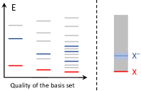
Figure 1: Description of an autodetaching anion X^- in a standard electronic-structure calculation. Left: When the size of the basis set is increased, the description of the continuum (gray) improves and the resonance (blue) cannot be associated with a single discrete state anymore. Right: In a complete basis set, the resonance can be associated with a peak in the density of continuum states. The onset of the electronic continuum is shown in red. Reproduced with permission from Ref. 69.

2.2 Core-vacant states

Electronic resonances are also encountered when moving beyond anions with the difference that the decay of neutral or cationic species is termed autoionization instead of autodetachment. Neutral states above the first ionization threshold are also called superexcited states. An important subgroup of autoionizing resonances consists in core-vacant states, which are created by interaction with X-rays in various spectroscopies.^{7, 8, 9} These techniques typically involve photon energies larger than 200 eV up to 1000 eV so that the resulting states are located at much higher energies than the temporary anions from Sec. 2.1.

Core-vacant states are subject to the Auger-Meitner effect,^{70, 71} in which the core vacancy is filled while a second electron is emitted into the ionization continuum. Different variants of Auger decay and the corresponding decay channels can be identified in Auger electron spectroscopy⁷ by measuring the kinetic energy of the emitted electrons. Several important non-radiative decay processes that can follow initial core ionization or core excitation,^{72, 73, 74, 75} are depicted in Fig. 2. Further related processes besides those in Fig. 2 include double Auger decay,⁷⁶ where two electrons are simultaneously emitted, and various shake-up and shake-off mechanisms,^{77, 78, 79} where an additional valence electron is ionized or excited, respectively. It is also common that the target states of Auger decay undergo further decay resulting in so-called Auger cascades.⁷

An important common aspect of core-vacant states is that they can be modeled as bound states with much better accuracy than other types of resonances. In particular, it is possible to project out the ionization continuum by means of the core-valence separation.^{21, 80, 81, 82} This is done by removing those configurations from the Hilbert space that describe the Auger decay. Notably, such decoupling is not possible for core-excited states above the respective core-ionization threshold (right panel of Fig. 2).

Related to Auger decay are non-local processes in which the emitted electron does not stem from the atom or molecule in which the core hole was located. The prime example is intermolecular Coulombic decay (ICD),⁸³ but there are further flavors such as electron-transfer mediated decay⁸⁴ and interatomic Coulombic electron capture.⁸⁵ ICD and related processes are possible at considerably lower energies than Auger decay and thus presumed to be more widespread.⁸⁶ Also, the efficiency of ICD increases in the presence of many neighboring molecules that can be ionized, which further contributes to its relevance in complex systems. It has even been claimed that ICD is everywhere.⁸⁷

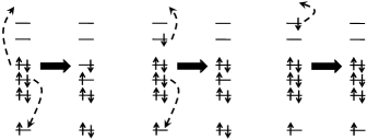
Figure 2: Non-radiative decay of core-vacant states: In Auger decay depicted in the left panel, a core-ionized cationic state decays into a dicationic state. In resonant Auger decay depicted in the middle, a core-excited neutral state decays into a cationic state. There are also core-excited states above the respective core-ionization threshold that can undergo a one-electron decay process in which the core hole is not filled as shown in the right panel.

2.3 Quasistatic ionization

A further type of electronic resonance, which is not connected to autodetachment or autoionization, arises when atoms or molecules are exposed to intense laser fields that are comparable in strength to the intramolecular forces. Under such conditions, quasistatic ionization takes place and bound states are turned into Stark resonances.^{15, 16} This process underlies many phenomena observed in strong laser fields, in particular high-harmonic generation.^{13, 14} While a comprehensive discussion of atoms and molecules in laser fields is beyond the scope of this article, a brief account of quasistatic ionization is given in the following.

One can distinguish alternating current (ac) Stark resonances formed in time-dependent electric fields and direct current (dc) Stark resonances formed in static electric fields. The formation of dc Stark resonances can be understood in terms of Fig. 3: Owing to the distortion of the potential, electrons can leave the system by tunneling. At even higher field strengths, electrons can leave above the barrier, which is termed barrier-suppression ionization.^{13, 88} Strictly speaking, tunnel ionization is already possible at infinitesimally low field strengths meaning that the Hamiltonian of a molecule in the presence of an external electric field never supports any bound states.^{89, 90, 91}

Figure 3: Distortion of a Coulombic potential by a static electric field in one dimension. A stable energy level (left) becomes metastable in the presence of a field (middle). At higher field strengths, barrier-suppression ionization is possible (right). Reproduced with permission from Ref. 92.

This effect can be ignored if the field strength is low enough and a treatment of light-matter interaction in terms of response properties is possible.⁹³ However, the radius of convergence of a perturbative expansion in powers of the field strength is determined by the tunnel ionization rate.⁹¹ At higher field strengths where decay widths are significant; a treatment of the external field as perturbation is not valid.

To determine under what conditions quasistatic ionization takes actually place, not only the field strength but also the frequency of a laser need to be considered.^{13, 14, 94} For small molecules in the electronic ground state, field strengths of the order of $10^{-4}$ to 1 a.u. are usually of interest. This exceeds field strengths typical for photochemistry by orders of magnitudes, the realization of such conditions is, however, no problem in modern laser experiments.^{13, 14} By means of Keldysh’s adiabaticity parameter, different ionization mechanisms can be distinguished.⁹⁵ This relates the tunneling time to a wave period and provides thus an estimate if the ionization can be thought of as static process as depicted in Fig. 3. If this is the case, the time dependence of the field can be neglected, hence the name quasistatic ionization.

This leads to a considerable simplification because one can work with a time-independent Hamiltonian. For the hydrogen atom, an estimate of the tunnel ionization rate was obtained already in 1928⁹⁶ and later refined and extended.^{97, 98, 99, 100, 101, 102, 103} The accurate evaluation of molecular quasistatic ionization rates has remained an active research field until today and is of relevance to many experiments where strong fields are applied. Especially the modeling of the angular dependence of the ionization rate is a challenge. This is caused by the exponential dependence of the ionization rate on the binding energy; in a polyatomic molecule the contribution of individual channels to the overall ionization rate varies greatly depending on orientation.^{104, 105, 106}

2.4 Shape and Feshbach resonances

One can group metastable electronic states into shape resonances, which decay by a one-electron process, and Feshbach resonances, which decay by a two-electron process.^{15, 17} The distinction is illustrated by Fig. 4 for autodetaching anions. Notably, polyatomic molecules usually feature resonances of both types. Examples of shape resonances include

• temporary radical anions formed by electron attachment to neutral ground states,^{57, 10, 11}

• low-lying excited states of closed-shell anions,^{57, 10, 11}

• most metastable dianions and more highly charged anions,⁶⁶

• some superexcited states of neutral molecules,^{107, 108}

• core-excited states above the respective core-ionization threshold,^{73, 74}

• Stark resonances formed in static or dynamic electric fields.^{109, 88, 13, 14, 110}

Examples of Feshbach resonances include

• core-ionized states that undergo Auger decay,^{70, 71, 7}

• core-excited states that undergo resonant Auger decay,^{72, 75}

• related species involving more than one molecule that decay through intermolecular Coulombic decay,^{83, 86}

• anionic states formed by electron attachment to Rydberg states,^{111, 112, 113}

• superexcited Rydberg states,^{107, 114, 115, 116}

• states of high spin multiplicity that decay only by spin-orbit coupling.^{117, 118, 119, 120}

Figure 4: Electronic structure of shape (left) and Feshbach (right) resonances. If the metastable S₁ state of the anion X^- lies above its decay channel D, the decay is a one-electron process. If it lies below state D of the neutral molecule and at the same time above another decay channel D’, the decay is a two-electron process.

Shape resonances can be easily understood in real coordinate space: The shape of the effective potential is responsible for the metastable nature of the resonance, meaning the electron is trapped behind a potential wall but it can leave the system by tunneling.¹⁵ In the case of radical anions this potential wall is given by the sum of the centrifugal potential and the molecular Coulomb potential,^{57, 11} whereas in dianions a repulsive Coulomb barrier is formed by the sum of short-range attractive valence interactions and long-range repulsion between every electron and the anionic rest.^{57, 11} For Stark resonances, the potential wall is formed through the combination of the molecular potential and the external field.¹³

For Feshbach resonances, decay by a one-electron process is energetically impossible. The metastability only originates from the coupling to another decay channel and involves more than one degree of freedom. Feshbach resonances are thus more naturally described in the space of electronic configurations.^{17, 15} They can be viewed as superposition of two wave functions one of which is a bound states while the other one has continuum character. This also forms the motivation for the theory by Fano and Feshbach^{40, 41} where one aims to decouple a Feshbach resonance from the continuum so that bound-state methods become amenable.

Owing to the stronger coupling to the continuum, shape resonances are, in general, shorter lived than Feshbach resonances.^{15, 17} However, this is not always the case because other factors influence the lifetime as well. Also, the character of a molecular resonance can vary across the potential surface as decay channels open or close.

3 Complex-variable techniques

3.1 General theory

Since electronic resonances belong to the continuum, they cannot be described as stationary solutions of the time-independent Schrödinger equation in Hermitian quantum mechanics. Complex-variable techniques based on non-Hermitian quantum mechanics^{17, 16, 15} offer the possibility to describe electronic resonances in terms of discrete eigenstates. On a qualitative level, it is easy to see that the so-called Siegert representation¹²¹

$$E=E_{R}-i\,\Gamma/2$$ (1)

describes a state with finite lifetime. The imaginary part of the energy leads to decay as the time evolution of the wave function shows:

$$\Psi_{\text{res}}(t)=\exp[-i\,E\,t]\cdot\Psi_{\text{res}}(0)=\exp[-i\,E_{R}\,t]\cdot\exp[-\Gamma\,t/2]\cdot\Psi_{\text{res}}(0)~{}.$$ (2)

The probability density thus evolves in time as $-\Gamma\,t$ and the resonance width $\Gamma$ is connected to the characteristic lifetime $\tau$ through $\Gamma=1/\tau$. Although there remain fundamental issues with non-Hermitian quantum mechanics that are yet to be solved, for example, the formulation of closure relations for non-Hermitian Hamiltonians,¹⁵ Eq. (1) offers conceptual simplicity and emphasizes the similarity between resonance and bound-state wave functions. This equation forms the basis for extending quantum chemistry of bound states to electronic resonances.

A more rigorous justification of Eq. (1) and the concept of complex-valued energies requires an analysis in terms of scattering theory, which is available, for example, in Refs. 15, 32, 33. The central quantity considered there is the scattering matrix $\mathbf{S}(k)$, which connects initial and final states of a system undergoing a scattering process, i.e., an electron-molecule collision in the case of electronic resonances. The poles of $\mathbf{S}(k)$ in the complex momentum plane, which represent the values of $k$ at which the amplitude of the incoming wave vanishes, can be associated with resonances and bound states as illustrated in Fig. 5.

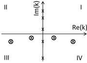
Figure 5: Schematic representation of the complex momentum plane. Poles of S on the positive Im(k)-axis correspond to bound states ($\times$) whereas resonances ($\otimes$) lie in the fourth quadrant. Poles on the negative Im(k)-axis and in the third quadrant are antibound states ($\times$) and capture resonances ($\otimes$), respectively. These states are in general beyond the reach of complex-variable methods and not discussed further here. However, note that antibound states are also referred to as virtual states and related to s-wave scattering.³²

Decaying resonances, meaning the poles of $\mathbf{S}(k)$ in the fourth quadrant in Fig. 5 are connected to peaks in the density of states in the continuum. The full width at half maximum $\Gamma$ of a peak centered at $E_{R}$ is given by Eq. (1) as can be derived by considering a closed contour integral in the lower half of the complex momentum plane^{15, 52}

$$N=\frac{1}{2\pi i}\oint_{C}\frac{\partial\text{ln}\mathbf{S}(k)}{\partial k}\mathrm{d}k$$ (3)

with $N$ as the number of poles in the lower half of the complex momentum plane, and applying the residue theorem to it. While a bound state with purely imaginary $k$ has an energy $E=k^{2}/2\in\mathbb{R}^{-}$, a $k$-value in the fourth quadrant leads to an energy

$$E=1/2\cdot[\text{Re}^{2}(k)-\text{Im}^{2}(k)-2\,i\,\text{Im}(k)\text{Re}(k)]~{}\in\mathbb{C}~{},$$ (4)

where the imaginary part is strictly negative. The comparison of Eqs. (1) and (4) shows that the location of a resonance in the complex momentum plane is directly related to its position and width, i.e., $E_{R}$ and $\Gamma$.

A resonance wave function corresponding to a pole of $\mathbf{S}(k)$ in the fourth quadrant in Fig. 5 behaves asymptotically, in the simplest case, like $\sim\exp[i\,\text{Re}(k)\,r]\;\exp[\text{Im}(k)\,r]$. This means that these wave functions diverge in space; they are thus outside the reach of quantum-chemical methods designed for $\mathcal{L}^{2}$ integrable states. Such outgoing boundary conditions as well as other boundary conditions used in scattering theory³² are difficult to implement into quantum-chemistry software.^{15, 122, 17, 39} An elegant solution is to regularize the diverging wave functions so that bound-state methods become applicable, which can be achieved by different techniques. Of interest to this article are complex scaling^{49, 50, 51, 53} and complex absorbing potentials,^{55, 56} which are discussed in Secs. 3.2 to 3.6. Both approaches lead to a non-Hermitian Hamiltonian with complex eigenvalues that can be interpreted according to Eq. (1) and with corresponding eigenfunctions that are $\mathcal{L}^{2}$ integrable.

Non-Hermitian Hamiltonians have, in general, different left and right eigenvectors.¹⁵ However, when working with complex scaling or complex absorbing potentials, it is possible to choose identical left and right eigenvectors if the Hamiltonian is real-valued before the complex-variable treatment is applied. This implies that the matrix representation becomes complex symmetric. As a consequence, the usual scalar product needs to be replaced by the so-called $c$-product^{15, 16, 123, 52}

$$\langle\Psi_{i}(r)|\Psi_{j}(r)\rangle=\int dr\,\Psi_{i}(r)\,\Psi_{j}(r)$$ (5)

where the state on the left is not complex conjugated. The $c$-product is sometimes denoted by round brackets $(\dots|\dots)$ instead of angle brackets $\langle\dots|\dots\rangle$ but this practice is not followed here to avoid confusion with Mulliken and Dirac notation for electron-repulsion integrals. Instead, angle brackets are kept and the use of the $c$-product is always implied when discussing complex-variable methods.

A further consequence of non-Hermiticity is the complex-variational principle,^{124, 123, 125}

$$\tilde{E}=\langle\tilde{\Psi}|H|\tilde{\Psi}\rangle/\langle\tilde{\Psi}|\tilde{\Psi}\rangle~{}\in\mathbb{C}$$ (6)

that holds for any $c$-normalizable trial wave function $\tilde{\Psi}$. Eq. (6) replaces the usual variational principle for all complex-variable methods alike and is a stationarity principle for the complex energy rather than an upper or lower bound for its real or imaginary part.

3.2 Formal aspects of complex scaling

Complex scaling^{15, 16, 49, 50, 51, 126, 127, 128, 52} is a mathematically rigorous technique to make diverging resonance wave functions $\mathcal{L}^{2}$ integrable. It represents a dilation transformation and relies on analytic continuation of the Hamiltonian to the complex plane. Analytic continuation is a mathematical technique to extend the domain over which an analytic function is defined. Upon scaling all coordinates in a Hamiltonian $H=T+V$ with $T$ as kinetic energy and $V$ as compact potential¹²⁶ by a complex number $e^{i\theta}$, $\theta\in\mathbb{R}$, $\theta<\pi/4$, a non-Hermitian operator $H^{\theta}$ is obtained with the spectral properties illustrated in the upper panels of Fig. 6:

• All discrete eigenvalues of $H$, that is, bound-state energies, are also eigenvalues of $H^{\theta}$.

• The continuous spectrum of $H^{\theta}$ is $\bigcup_{E_{t}}+ae^{-2i\theta}$, $a\in\mathbb{R}^{+}$ where $E_{t}$ are the thresholds of $H$, that is, in the context of electronic-structure theory the ionization energies if one deals with a neutral molecule and the detachment energies for an anion. Note that, for $H^{\theta}$, there are separate continua that correspond to the different thresholds and associated decay channels, whereas there is just one continuum for $H$.

• $H^{\theta}$ may have discrete complex eigenvalues in the wedge formed by the continuous spectra of $H$ and $H^{\theta}$. These can be associated with the resonances.

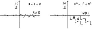
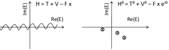
Figure 6: Upper panels: Eigenvalue spectra of a Hamiltonian $H=T+V$ describing an autoionizing resonance and of its complex-scaled counterpart $H^{\theta}$. Lower panels: Eigenvalue spectra of a Hamiltonian $H=T+V-Fx$ describing ionization in a static electric field and of its complex-scaled counterpart $H^{\theta}$. Continua are denoted by $\sim\!\!\sim$, bound states by $\times$, and resonances by $\otimes$. Note that the potential $V-Fx$ does not support any bound state.

A resonance wave function with the asymptotic behavior $\sim\exp[ikr]$, $k\in\mathbb{C}$ becomes $\mathcal{L}^{2}$ integrable upon complex scaling if $\theta>1/2\;\text{atan}[\Gamma/2\,(E_{R}-E_{t})]$. Above the same critical value, the resonance energies are independent of $\theta$. Since complex scaling relies on analytic continuation, the original theory^{49, 50} is only applicable to Hamiltonians with dilation-analytic potentials. Such potentials can be loosely defined as being analytic in the parameter of the dilation transformation, that is, $e^{i\theta}$ in the case of complex scaling. A rigorous definition of dilation analyticity is given in Refs. 49 and 126.

Whereas it has been established that the Coulomb potential is dilation analytic, an important case of a non-analytic potential is $V(x)\sim x$,^{109, 129, 89, 90, 130, 88} which describes a static electric field in $x$ direction. This implies that a Hamiltonian for an atom or molecule in a field has other spectral properties;^{129, 89, 90} these are illustrated in the lower panels of Fig. 6:

• Neither $H$ nor $H^{\theta}$ have discrete real eigenvalues, that is, bound states.

• The continuous spectrum of $H$ comprises the whole real axis, whereas the continuous spectrum of $H^{\theta}$ is empty.

• $H^{\theta}$ may have discrete complex eigenvalues. These can be associated with Stark resonances.

Although $V(x)\sim x$ is not dilation analytic, complex scaling renders Stark resonances, which asympotically behave as Airy functions, $\mathcal{L}^{2}$ integrable.

3.3 Complex scaling in the context of molecular electronic-structure theory

While implementations of complex scaling in which the wave function is represented on a numerical grid preserve many of the appealing formal properties of the exact theory,^{131, 132, 133, 134} the representation in a basis set of atom-centered Gaussian functions suffers from several problems:⁶⁷ The discrete eigenvalues of $H^{\theta}$ become $\theta$-dependent, whereas only the rotated continua depend on $\theta$ in the exact theory. This poses a problem for the computation of interstate properties as two states can depend on $\theta$ in a different way. A further problem arises for Stark resonances because the continuous spectrum is empty as illustrated in the lower panels of Fig. 6. The projection of $H^{\theta}$ onto a finite basis set therefore gives rise to additional unphysical eigenvalues that do not correspond to either bound, resonance, or continuum states.⁹²

The dependence of the bound-state and resonance energies on $\theta$ can be traced back to an oscillatory behavior $\sim\exp[-i\,Z\,r\sin\theta]$ of the respective wave functions that is introduced by complex scaling.¹³⁵ Importantly, this dependence of the wave functions on $\theta$ is also present in exact theory, but since it is difficult to represent in Gaussian bases, it gives rise to an artificial $\theta$-dependence of the energies in this case. The magnitude of the perturbation is best quantified by analyzing bound states for which $\text{Im}(E)$ is strictly zero in exact theory but of the order of $10^{-4}-10^{-3}$ a.u. in typical calculations in Gaussian basis sets.^{67, 92, 136}

$\theta$-dependence entails the need to find an optimal value, $\theta_{\text{opt}}$, which is usually done using the criterion^{124, 123, 52}

$$\text{min}\;[dE/d\theta]$$ (7)

because this derivative vanishes in exact theory. Eq. (7) works equally well for temporary anions, core-vacant states, as well as Stark resonances. A step size of $1^{\circ}$ for $\theta$ is usually adequate to evaluate Eq. (7) to sufficient accuracy. In addition, $\theta$ is confined to the interval $0<\theta<\pi/4$ by theory and varies little among resonances with similar electronic structure and among different electronic-structure methods. A more pronounced dependence on the basis set is, however, sometimes observed. In effect, this means that ca. 10–15 calculations need to be performed to determine $\theta_{\text{opt}}$ if no information can be inferred from preceding investigations. This is the main reason for the increased computational cost of complex-scaled calculations. Further reasons are the use of complex algebra and the need to include additional diffuse functions in the basis set; standard bases typically yield bad results.^{67, 92, 17, 136} While there are basis sets that have been designed specifically for resonances,^{137, 138, 139} the addition of a few shells of even-tempered diffuse functions to a standard basis usually works as well.^{67, 17}

3.4 Complex basis functions

Complex scaling in its original formulation is limited to atomic resonances, because the electron-nuclear attraction is not dilation analytic within the Born-Oppenheimer (BO) approximation.^{15, 17} However, because only the asymptotic behavior of the resonance wave function matters for the regularization, the non-analyticity can be circumvented by so-called exterior complex scaling (ECS),^{140, 141, 142} where only the outer regions of space, where the electron-nuclear attraction vanishes, are complex scaled. ECS has been implemented for a number of time-dependent approaches in which the wave function is represented on a numerical grid.^{131, 132, 133, 143, 134, 144, 145, 146, 147, 148, 149} Such approaches hold a lot of promise but the realization of ECS in basis set of atom-centered Gaussians is difficult because most techniques for AO integral evaluation are not applicable to the ECS Hamiltonian.

To implement ECS in the context of Gaussian basis sets, one can exploit the identity

$$E=\frac{\langle\Psi(r)|H^{\theta}(r\,e^{i\theta})|\Psi(r)\rangle}{\langle\Psi(r)|\Psi(r)\rangle}=\frac{\langle\Psi(r\,e^{-i\theta})|H(r)|\Psi(r\,e^{-i\theta})\rangle}{\langle\Psi(r\,e^{-i\theta})|\Psi(r\,e^{-i\theta})\rangle}~{},$$ (8)

that is, scaling the coordinates of the Hamiltonian as $r\to re^{i\theta}$ is equivalent to scaling the basis in which the Hamiltonian is represented as $r\to re^{-i\theta}$.^{53, 54} The right-hand side of Eq. (8) is equivalent to scaling the exponents of Gaussian basis functions by $e^{-2i\theta}$.⁵³ If one does not apply this procedure to all basis functions but rather adds to a given basis set a number of extra functions with complex-scaled exponents,

$$\chi_{\mu}(r,A)=N_{\mu}(\theta)\,S_{\mu}(r_{A})\,\text{exp}\big{[}-\alpha_{\mu}\,e^{-2i\theta}\,r_{A}^{2}\big{]}~{},$$ (9)

a basis-set representation of ECS is obtained. Alternatively, the functions from Eq. (9) can be interpreted as being centered not at the nuclei but in the complex plane. The so-defined complex basis function (CBF) method^{53, 150, 151, 152, 153, 154, 155, 156, 157} is compatible with the BO approximation; its main technical challenge consists in the need to evaluate integrals over the non-standard basis functions from Eq. (9).¹⁵⁵ Whereas most of the established techniques for AO integral evaluation apply to complex exponents, several changes are necessary for the computation of the Boys function, which forms the first step of the evaluation of the electron-repulsion integrals; an efficient implementation was introduced only recently.¹⁵⁵

Besides the applicability to molecules, CBF methods offer further advantages over complex scaling of the Hamiltonian: $\text{Im}(E)$ of bound states is typically much smaller (ca. $10^{-5}$ a.u.) indicating a better representation of the complex-scaled wave function. Also, while an optimal scaling angle $\theta_{\text{opt}}$ needs to be determined using Eq. (7), the values of $dE/d\theta$ are significantly smaller than when the Hamiltonian is complex-scaled. The requirements of CBF calculations towards the basis set are, in general, somewhat less arduous than those of complex scaling, although it is necessary to augment standard bases by extra functions. The details depend on the type of resonance and the energy released in the decay process.^{155, 156, 157, 104, 136}

3.5 Formal aspects of complex absorbing potentials

Complex absorbing potentials (CAPs) have been used for long in quantum dynamics as a means to prevent artificial reflection of a wave packet at the edge of a grid.¹⁵⁸ By accident, it was discovered that CAPs are also useful in static electronic-structure calculations.⁵⁵ By absorbing the diverging tail of the wave function, a CAP enables an $\mathcal{L}^{2}$ treatment of resonances similar to complex-scaled approaches. More thorough analysis showed that CAPs are, under certain conditions, mathematically equivalent to complex scaling.^{56, 159, 160, 161} If this is the case, exact resonance positions and widths can be recovered from CAP calculations. Still, in practice, CAP methods feature more heuristic aspects than complex-scaled methods as will be detailed in this section and the subsequent one. At the same time, CAPs are easier to integrate into molecular electronic-structure theory.^{17, 162} In particular, no difficulties arise about the combination with the BO approximation so that CAP methods can be readily applied to molecules.

The CAP-augmented Hamiltonian is given as

$$H^{\eta}=H-i\;\eta\;W$$ (10)

with $\eta\in\mathbb{R}^{+}$ as strength parameter. Different functional forms have been suggested for $W$,^{56, 159, 160, 161, 163, 164, 165, 166, 162, 167, 168} in the simplest case $W$ is chosen as a real-valued quadratic potential of the form

$$W=\!\!\sum_{\alpha=x,y,z}\!\!W_{\alpha}\,,~{}\;W_{\alpha}=\begin{cases}(|r_{\alpha}-o_{\alpha}|-r_{\alpha}^{0})^{2}&\text{if}~{}|r_{\alpha}-o_{\alpha}|>r_{\alpha}^{0}\\ 0&\text{if}~{}|r_{\alpha}-o_{\alpha}|<r_{\alpha}^{0}\end{cases}~{}.$$ (11)

Here, the vector $(r_{x}^{0},r_{y}^{0},r_{z}^{0})$ defines the onset of the CAP and hence a cuboid box in which the CAP is not active and the vector $(o_{x},o_{y},o_{z})$ is the origin of the CAP. $r_{\alpha}^{0}$ and $o_{\alpha}$ are heuristic parameters, protocols for their determination are discussed in Sec. 3.6.

A suitable starting point for the mathematical analysis of $H^{\eta}$ is a free particle in one dimension exposed to a CAP with onset $r_{x}^{0}=0$.^{56, 169} In this case, $H$ comprises only kinetic energy and the operator

$$H^{\eta}=-\frac{1}{2}\frac{\partial}{\partial x^{2}}-i\,\eta\,x^{2}$$ (12)

describes a harmonic oscillator with frequency $\sqrt{\eta}\,(1-i)=\sqrt{2\eta}\,\text{exp}[-i\pi/4]$ on a complex-rotated length scale $(2\,\eta)^{-1/4}\,\text{exp}[i\,\pi/8]$. The spectrum of eigenvalues is $E_{n}=\sqrt{\eta}(1-i)\,(n+1/2),\;n\in\mathbb{N}$, that is, it is rotated into the lower half of the complex energy plane by an angle of $2\theta=\text{exp}[-i\,\pi/4]$ mimicking complex scaling with $\theta=\pi/8$. At the same time, the spectrum of $H^{\eta}$ is purely discrete for finite $\eta$; the continuous spectrum of the complex-scaled Hamiltonian (see upper panels of Fig. 6) is recovered only in the limit $\eta\to 0^{+}$. By similar considerations it is possible to show that general monomial CAPs $W\sim r^{n}$ correspond to complex scaling with an angle $\theta=-\pi/(2+n)$.⁵⁶ Inclusion of a compact potential in $H^{\eta}$ does not fundamentally change this analysis.

CAPs of a more elaborate form than Eq. (11) have been investigated as well.^{159, 160, 52, 163, 164} One guiding principle has been to design potentials that are equivalent to complex scaling not only in the limit $\eta\to 0^{+}$ but also for finite values of $\eta$. As a first step, one can choose $\eta$ to be energy-dependent because it can be shown that reflection and absorption properties depend on the energy as well. Applying the ansatz $\eta(E)=2\,a\,(E-V)$ to Eq. (10) leads to a modified Schrödinger equation¹⁵⁹

$$T|\Psi(x)\rangle+V(x)\,(1+2i\,a\,W(x))|\Psi(x)\rangle=E(1+2i\,a\,W(x))|\Psi(x)\rangle$$ (13)

which can be recast in the usual form by introducing the function $f=\sqrt{1+2i\,a\,W}$. This results in

$$f^{-1}\,T\,f^{-1}\,|\widetilde{\Psi}(x)\rangle+V(x)|\widetilde{\Psi}(x)\rangle=E|\widetilde{\Psi}(x)\rangle$$ (14)

with $|\widetilde{\Psi}(x)\rangle=f\,|\Psi(x)\rangle$ as transformed wave function. Eq. (14), which features a modified kinetic energy, illustrates the connection between CAPs and ECS; it can be shown that the function $f$ defines a scaling contour in the complex plane. Since the theory of complex scaling places only few restrictions on the scaling contour,^{15, 52} that is, the path in the complex plane along which the coordinates are scaled, diverse functional forms of $W$ are possible. This connection between CAPs and ECS has triggered the development of the transformative CAP^{159, 160} (TCAP) and of several reflection-free CAPs^{159, 160, 161, 164} all of which are built around a transformed kinetic energy. The TCAP has been implemented for a few electronic-structure methods,¹⁶⁸ which showed that, despite formal advantages over Eq. (11), the results still suffer from the same shortcomings when using atom-centered Gaussian basis sets. Most recent developments are thus built on the simpler functional form from Eq. (11).

3.6 Complex absorbing potentials in the context of molecular electronic-structure theory

While the limit $\eta\to 0^{+}$ can be taken if the Schrödinger equation is solved exactly, this is not the case when $H^{\eta}$ is represented in a finite basis set and the Schrödinger equation is solved approximately.⁵⁶ Instead, one has to use finite $\eta$ values and balance out two effects: The error caused by the finite CAP strength, which increases with $\eta$ and an additional error $\Delta E_{\text{bas}}(\eta)$ caused by the finite basis set, which decreases with $\eta$. The optimal value $\eta_{\text{opt}}$ is usually determined by a Taylor expansion of the resonance energy in $\eta$

$$E(\eta)=E_{0}+a_{1}\eta+a_{2}\eta^{2}+a_{3}\eta^{3}+\dots+\Delta E_{\text{bas}}(\eta)$$ (15)

and minimizing the linear term, which leads to the criterion⁵⁶

$$\text{min}\,|\eta dE/d\eta|~{}.$$ (16)

In analogy to complex-scaled methods, this entails the need to calculate trajectories $E(\eta)$. However, CAP theory does not place an upper limit on $\eta$, whereas the complex scaling angle is restricted to $0<\theta<\pi/4$. In practice, $\eta_{\text{opt}}$ varies from $10^{-4}$ to $10^{-1}$ a.u. between different calculations depending on the completeness of the basis set and the choice of onset $(r_{x}^{0},r_{y}^{0},r_{z}^{0})$ and origin $(o_{x},o_{y},o_{z})$ so that, typically, between 20 and 50 calculations need to be run to determine the optimal CAP strength.^{17, 162, 170}

For temporary anions, a possible choice for the onset that avoids optimization on a case-by-case basis consists in $\sqrt{X^{2}}$, $\sqrt{Y^{2}}$, $\sqrt{Z^{2}}$ where the expectation values are computed for the neutral ground state.^{162, 170, 171, 172} This approach aims to minimize the perturbation of the neutral system and to apply the CAP only to the extra electron. It is, however, not straightforward to generalize the idea to other types of resonances beyond temporary anions. As an alternative, the definition of the CAP onset on the basis of Voronoi cells has been suggested.^{167, 173} This in advantageous for larger molecules of irregular shape where the definition of a CAP according to Eq. (11) is questionable. In other cases, Voronoi CAPs and box-shaped CAPs deliver very similar results. The impact of the CAP origin has been investigated less thoroughly, it is usually chosen as the center of mass or the center of nuclear charges of a molecule.^{162, 174, 175}

While the integrals $W_{\mu\nu}=\langle\chi_{\mu}|W|\ \chi_{\nu}\rangle$ of a box-shaped CAP defined according to Eq. (11) over Gaussian functions can be calculated analytically,¹⁷⁶ the corresponding integrals of a Voronoi CAP need to be evaluated numerically.¹⁶⁷ However, the evaluation of integrals over arbitrary potentials is a standard task in density functional theory and adapting such functionalities to the evaluation of CAPs is straightforward.¹⁶² In general, the evaluation of $W_{\mu\nu}$ does not drive the computational cost.

In analogy to complex-scaled and CBF calculations, additional shells of diffuse functions need to be added to a basis set to represent the resonance wave function properly in a CAP calculation. The same basis sets usually work as well but it is sometimes possible to truncate the basis set based on physical considerations when using CAPs.^{17, 162} For example, temporary anions that arise from adding an electron to a $\pi^{*}$ orbital can often be described with a basis set that includes only additional $p$ functions. However, a general observation is that the use of too small basis sets in CAP calculations gives rise to additional spurious minima in Eq. (16) that do not correspond to physical resonance states.^{171, 162, 17}

Several ideas have been proposed to reduce the dependence of the resonance energy on the CAP parameters. One can, for example, compute the linear term in Eq. (15) explicitly and subtract it from the energy.^{56, 171} This leads to the first-order corrected energy

$$E^{(1)}(\eta)=E(\eta)-\eta\,dE/d\eta=E+i\,\eta\,\langle W\rangle~{},$$ (17)

where the correction term is given as the expectation value of the CAP operator. $\eta_{\text{opt}}$ can be determined for Eq. (17) by minimizing the next-higher order term in Eq. (15), which leads to the criterion $\text{min}|\eta\,dE^{(1)}/d\eta|$. However, the correction leads to an increased basis-set error $\Delta E_{\text{bas}}(\eta)$ so that it is not guaranteed that $E^{(1)}$ represents an improvement over the uncorrected energy $E$.⁵⁶ In practice, this can be tested by comparing the values of $|\eta\,dE/d\eta|$ and $|\eta\,dE^{(1)}/d\eta|$, which shows that, in general, Eq. (17) does represent an improvement. The first-order corrected energy is less dependent on $\eta$ and the CAP onset than the uncorrected energy.^{171, 172, 17}

As an alternative to the Taylor expansion in Eq. (15), it has been suggested to express $E(\eta)$ in terms of Padé approximants.^{177, 178, 179} This allows to recover the non-analytic limit $\eta\to 0^{+}$ from a series of calculations with different $\eta$ values; the dependence of the energy on $\eta$ is, however, also with this approach not removed completely.

Recently, the integration of CAPs into Feshbach-Fano theory has been suggested¹⁸⁰ in order to define the projector needed there for separating bound and continuum parts of the wave function. In analogy to other approaches based on this theory, the computational cost is lower as compared to complex-variable methods because the Schrödinger equation is solved with a real-variable electronic-structure method and the CAP is added afterwards. However, only very few applications of this approach have been reported so far.¹⁸⁰

3.7 Practical aspects of complex-variable electronic-structure calculations

The choice of electronic-structure model is of central importance for the accurate description of molecular resonances. Complex scaling and complex absorbing potentials have been combined with a variety of methods; implementations of Hartree-Fock (HF),^{150, 151, 156} density functional theory (DFT),^{181, 182, 183},multireference configuration interaction (MRCI),^{168, 165, 153, 154} resolution-of-the-identity second-order Møller-Plesset perturbation theory (RI-MP2),^{105, 106} extended multiconfigurational quasidegenerate perturbation theory (XMCQDPT2),¹⁸⁴ algebraic diagrammatic construction (ADC),^{185, 186, 187, 188} symmetry-adapted-cluster configuration interaction (SAC-CI),¹⁸⁹ multireference coupled-cluster (MRCC),¹⁹⁰ and equation-of-motion (EOM)-CC methods^{166, 67, 162, 157} have been reported. Since there exist different ways to set up a complex-variable calculation, the comparison of results obtained using different implementations is not straightforward. Moreover, many approaches are specifically designed for the treatment of a particular type of resonance, i.e., only suitable for temporary radical anions, core-vacant states, or molecules in static electric fields. This has led to a situation where many resonances have been investigated with only one or two computational approaches. Systematic benchmarks, where the same resonances are computed using the same basis sets and complex-variable techniques but different electronic-structure models are still largely missing. The same applies to the numerical comparison of CAPs and complex scaling calculations based on the same electronic-structure model.

A first requirement towards a complex-variable electronic-structure model is that the wave function comprises configurations that describe the decay of the state. This is usually easy to achieve for shape resonances but requires more consideration in the case of Feshbach resonances. For example, the configurations describing Auger decay of a core-ionized state are doubly excited with respect to the core-vacant HF determinant (see Fig. 2); as a consequence, the decay cannot be described with HF theory.

A second requirement is to achieve a consistent description of the resonance itself and its decay channels.¹⁹¹ Multistate methods such as EOM-CC,^{192, 193, 194, 195, 196, 197, 198, 199, 200} CC2,^{201, 202, 203} and ADC(n),^{204, 205, 206, 207} which deliver wave functions for states with $N$ and $N+1$ electrons within the same computation, have a built-in advantage because they place the ionization continua such that no ambiguity over the character of a state arises. In contrast, if one performs, for example, two separate HF calculations for a temporary radical anions and the corresponding neutral molecule, it can happen that the decay width of the anion is zero although its HF energy is higher than that of the neutral species. This is further discussed in the context of analytic-gradient theory in Sec. 4.4.

Another advantage of multistate methods is the straightforward evaluation of transition moments as well as Dyson orbitals⁶⁸ and natural transition orbitals (NTOs).²⁰⁸ These quantities are equally relevant for resonances as for bound states;²⁰⁹ for example, they enable the application of exciton theory to resonances, which helps explain spectroscopic signatures of resonances.²⁰⁸ As a consequence of Eq. (5),the real and imaginary parts of orbitals need to be interpreted separately in the context of complex-variable methods. A representative example of an NTO pair is shown in Fig. 7.

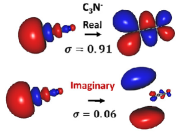
Figure 7: Real and imaginary NTOs and their corresponding singular values $\sigma_{K}$ for the ${}^{3}\Pi$ state of C₃N^- computed with CAP-EOM-EE-CCSD. Reproduced with permission from Ref. 208.

A further advantage of multistate methods is technical but crucial for some types of states: It is often possible to avoid solving the SCF equations for the resonance. Especially for temporary radical anions, it can be very difficult to ensure convergence to the resonance state instead of a pseudocontinuum solution. For other types of resonances, however, this is less problematic. For example, CBF-HF determinants for a core-vacant state or a molecule in a static electric field can be easily constructed using maximum-overlap techniques²¹⁰ starting from a real-valued core-vacant HF determinant or a field-free HF determinant, respectively.^{92, 104, 136}

It also needs to be mentioned here that the strengths and weaknesses that have been established for a particular electronic-structure method in the context of bound states, are still relevant for resonances. For example, many resonances have open-shell character, a spin-complete description as afforded by multistate methods such as EOM-CC and ADC is advantageous.

From these considerations, a number of computational approaches arise that combine several advantages for different types of resonances: For temporary radical anions, EOM-EA-CC within the singles and doubles approximation (EOM-EA-CCSD) based on a CCSD reference for the neutral closed-shell state is well suited or, alternatively, the EA variant of ADC(2) or ADC(3) starting from an MP2 or MP3 reference. Likewise, excited states of closed-shell anions, superexcited Rydberg states, and core-excited states are best described with the EE variants of the same methods, while the IP variants are suitable for core-ionized states.

For other types of states, a fully satisfactory description is more difficult to achieve: For example, in the case of closed-shell dianions, one can construct a CBF-HF or CAP-HF determinant for the resonance, treat correlation by means of CCSD, and describe the detachment channels as EOM-IP-CCSD states.²¹¹ This delivers a balanced and spin-complete description of all relevant states but the bound monoanionic states, which are described using orbitals of the resonance state, will likely have substantial non-zero imaginary energies. The alternative approach, where one starts from an open-shell HF determinant for one of the monoanionic decay channels, avoids the latter problem but delivers a description that is neither balanced nor spin-complete. A similar problem exists for Stark resonances where the Hamiltonian does not feature any bound states; it is thus inevitable to solve the SCF equations directly for the resonance.^{92, 104}

In post-HF CAP methods, a further degree of freedom arises because the CAP does not need to be added to the Hamiltonian from the outset. For example, in a CAP-EOM-CC treatment, the CAP can be introduced already in the HF calculation,^{162, 170} or at the CC step, or even only at the EOM-CC step.¹⁶⁶ No such choice exists for CBF methods and one needs to work with a complex-valued wave function throughout. In the full CI limit, all three variants of CAP-EOM-CC deliver identical results but this is not the case for truncated CC methods. The distinction between relaxed and unrelaxed (EOM-) CC molecular properties²¹² is related to this subject and, similar to what applies there, the numerical differences between the three CAP-EOM-CC variants are usually small.

Also, there is no clear formal advantage of one scheme over the other: If the CAP is active already at the HF level, the form of the CC and EOM-CC equations does not change as compared to the real-valued formalism. Also, the size-extensivity of truncated CC methods is preserved and it is straightforward to work out analytic-derivative theory (see Sec. 4.4). The main advantage of the alternative variant in which the CAP-EOM-CC Hamiltonian is built from a real-valued CC wave function is its reduced computational cost. Only the EOM-CC equations have to be solved for multiple values of the CAP strength to evaluate Eq. (16), the CC equations for the reference state need to be solved only once. However, these methods are not size-intensive and it is necessary to include additional terms in the EOM-CC equations because the cluster operator does not fulfill the CC equations at $\eta\neq 0$.

As a further idea in the context of temporary radical anions, it has been suggested to project the CAP on the virtual orbital space.²¹³ The rationale is to minimize perturbation of the occupied orbital space and to apply the CAP only to the extra electron. This has been realized for CI and EOM-CC methods;^{213, 166, 17} numerical evidence suggests that the impact on the results is small.

Finally, it should be mentioned that there is some ambiguity in the evaluation of Eqs. (7) and (16) as one can search for minima in the total resonance energy or in the energy difference with respect to some bound parent state.^{67, 157} If the Schrödinger equation was solved exactly, this would not matter because bound-state energies do not depend on the complex scaling angle or the CAP strength in that case. However, it can matter for approximate solutions, in particular for calculations with a complex-scaled Hamiltonian where bound states acquire substantial imaginary energies (see Sec. 3.3). For CBF calculations, the impact is substantially smaller. Numerical experience shows that Eq. (7) is best applied to energy differences here.^{157, 104, 136} For CAP calculations, the differences are usually negligible.

4 Recent methodological developments

4.1 Complex-valued potential energy surfaces and analytic gradient theory

The concept of potential energy surfaces (PES) is a cornerstone of the quantum chemistry of bound states. By virtue of the BO approximation, the electronic energy is obtained as a function of the nuclear coordinates by solving the electronic Schrödinger equation at fixed nuclear positions. The nuclear dynamics are then described in terms of these PES.

Consideration of nuclear motion is equally important for molecular electronic resonances because it happens in many cases on the same timescale as electronic decay. As an example, consider DEA to a closed-shell molecule. The cross section for this process is determined by the interplay of nuclear motion and electronic decay.⁵⁸ Moreover, there are important cases of DEA where two electronic resonances are coupled through nuclear motion^{214, 215}. Aside from DEA, there are anions whose autodetachment is entirely due to nuclear motion,^{216, 217, 218} for example NH^-219 and enolates,²²⁰ as well as other anions that are adiabatically bound only when zero-point vibrational energies are taken into account, for example benzonitrile.²²¹ Vibrational effects hence play a decisive role for the spectroscopy of temporary anions,¹⁰ but also for other types of resonances such as core-vacant states.⁸

Using the Siegert representation, Eq. (1), the concept of PES can be readily generalized to resonances: The real part of the PES is interpreted in analogy to bound states, whereas the imaginary part yields the decay width as a function of the molecular structure.²²² Complex-valued resonance PES can be as diverse as those of bound states but the former are in general much less well characterized than the latter. Fig. 8 illustrates several typical PES shapes for temporary radical anions. These resonances often become stable towards electron loss through structural changes, typically through bond stretching.¹⁷ However, such stabilization does not pertain to most other types of resonances: A molecule in a static electric field does not have any bound states so that the electronic energy remains complex-valued at all nuclear configurations. The same applies to core-vacant states, which also do not become bound through structural rearrangement.

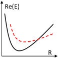
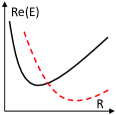
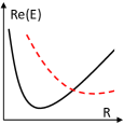
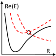
Figure 8: Exemplary shapes of potential energy surfaces of temporary anions in one dimension. Dashed red lines denote anionic states, solid black curves denote neutral states. Upper left: The anion is unbound but vertically stable at stretched bond lengths. (Example: N${}_{2}^{-}$) Lower left: The anion is vertically stable at its own equilibrium structure but adiabatically unbound (Example: CO${}_{2}^{-}$) Upper right: The anion is adiabatically bound but vertically unstable near the equilibrium structure of the parent neutral state. (Example: F${}_{2}^{-}$) Lower right: Dissociative electron attachment is possible and proceeds through coupling of two resonances. The exceptional point is marked by a circle. (Example: HCN^-)

Plots such as those in Fig. 8 cannot represent the full dimensionality of the PES for systems with more than two atoms; they can be exact only for diatomic molecules. An $N$-atomic molecule has $M=3N-6$ internal nuclear degrees of freedom ($3N-5$ for linear molecules); the PES is thus a high-dimensional object. In these cases, plots such as those in Fig. 8 only represent cuts through the PES and do not capture the full dimensionality. Although low-dimensional models can afford meaningful insights, it is desirable to treat all $M$ degrees of freedom on an equal footing as is routinely possible for bound states.

Bound-state PES are commonly characterized in terms of special points such as equilibrium structures, transition structures, conical intersection seams, and minimum energy crossing points (MECPs).^{223, 224, 225} Analogous special points on complex-valued PES are of interest for resonances as well. Equilibrium structures are characterized by $dE_{R}/d\mathbf{R}=0$ and positive real parts of all eigenvalues of the Hessian matrix; $\Gamma$ is not relevant here.

Crossing seams between a temporary anion and its parent neutral state mark the region where the anion becomes stable towards electron loss. Since the two states involved in such a crossing have a different number of electrons, the Hamiltonian does not couple them and the crossing seam has the dimension $M-1$. If $E_{R}$ and $E_{0}$ are obtained as eigenvalues of the same Hamiltonian, as is possible, for example, with EOM-CC or ADC methods, $\Gamma$ in principle becomes zero exactly at this crossing seam,¹⁹¹ which is not the case if $E_{R}$ and $E_{0}$ are computed independent of each other. However, since very small decay widths are difficult to represent with CAP methods, deviations are observed in practice also for multistate methods.²²⁶

The crossing seam between a temporary anion and its parent state can be related to the stability of a molecule towards low-energy electrons and the efficiency of DEA in a similar way in which the location and topology of a conical intersection explain photostability. Along the seam, the MECP is of particular interest, which motivated the development of an algorithm for locating it.²²⁶ In a straightforward extension of a similar algorithm for bound states,²²⁷ this can be done using the condition²²⁶

$$d/d\mathbf{R}\Big{[}E_{R}-E_{0}\Big{]}^{2}=0$$ (18)

and at the same time minimizing the energy of one of the states in the space orthogonal to the crossing seam.

Also of interest are crossing seams between two resonances. The intersection space where the real and imaginary parts of the energies are degenerate is termed exceptional point (EP).^{228, 229} As for conical intersections, the dimension of an EP seam is $M-2$,^{228, 230} which implies that diatomic molecules cannot feature EPs. More general intersection spaces, where only the real or imaginary parts of the energies are degenerate, can also be defined. The analogy between EPs and conical intersections does not reach very far: Although the dimension of the intersection space is the same, most other properties are fundamentally different. In particular, a non-Hermitian Hamiltonian is defective at an EP, which is not the case for a Hermitian Hamiltonian at a conical intersection.²²⁹

Although the role of EPs for molecular electronic resonances has not yet been investigated in a systematic manner,^{231, 214, 215, 232, 233, 230} it is clear that they are relevant to all processes that involve two coupled resonances. This is, for example, the case for DEA to unsaturated halogenated compounds, which is presumed to lead initially to a $\pi^{*}$ resonance that is coupled to a $\sigma^{*}$ resonance whose PES is dissociative.^{58, 215, 234, 235, 230} In analogy to bound states, non-adiabatic transitions are most likely to occur at the EP seam and especially near minimum-energy exceptional points (MEEPs). This motivated the development of an algorithm for locating MEEPs. This is again based on a generalization of the bound-state algorithm²²⁷ and uses the condition²³⁰

$$d/d\mathbf{R}\Big{[}(E_{R1}-E_{R2})^{2}+1/4\cdot(\Gamma_{1}-\Gamma_{2})^{2}\Big{]}=0~{},$$ (19)

where $E_{R1}$ and $E_{R2}$ are the positions of the two resonances and $\Gamma_{1}$ and $\Gamma_{2}$ the corresponding widths. In addition to Eq. (19), $E_{R1}$ or $E_{R2}$ needs to be minimized in the space orthogonal to the EP seam.

As a numerical example, Fig. 9 displays the PES of two resonances of HCN^- near their MEEP. This shows that CAP-EOM-CCSD describes the topology of EPs consistent with analytical models:^{214, 215} Square-root energy gaps are separately observed for the real and imaginary parts of the energy in the branching plane. Notably, standard EOM-CCSD yields a flawed description of conical intersections, where the dimensionality of the intersection space is incorrect;^{4, 5, 236} this difference between EOM-CCSD and CAP-EOM-CCSD can be traced back to fundamental differences between Hermitian and non-Hermitian operators.²³⁰

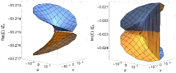
Figure 9: Real (right) and imaginary (left) parts of the PES of the ${}^{2}\Pi$ and the ${}^{2}\Sigma^{+}$ resonance of HCN^- computed with CAP-EOM-EA-CCSD. The EP is marked by a red dot. Reproduced with permission from Ref. 230.

In order to locate equilibrium structures as well as crossing seams using Eqs. (18) and (19), the first derivative of the complex resonance energy with respect to nuclear coordinates is required. In accordance with the interpretation of Eq. (1), the real part and imaginary part of the gradient vector describe the change in the energy and decay width across the PES. They point, in general, in different directions.

For diatomic and triatomic molecules, it is possible to evaluate the gradient vector through single-point energy calculations and numerical differentiation but such an approach becomes quickly impractical for polyatomic systems owing to increasing computational cost. For bound states, it was realized more than 50 years ago that an analytic evaluation of the energy gradient can be achieved at a cost similar to that associated with the evaluation of the energy itself.²³⁷ Since then, analytic-derivative theory has become an important aspect of quantum-chemical method development and gradient expressions have been derived for most of the frequently used electronic-structure methods.^{212, 93}

Corresponding developments for electronic resonances started only recently with the presentation of analytic gradients for CAP-HF, CAP-CCSD, and CAP-EOM-CCSD energies.¹⁷⁴ Because all AO integrals are real-valued in CAP methods, the evaluation of the energy is easier here than for CBF methods. In a generic gradient expression written in the AO basis,

$$\frac{dE}{dX}=\sum_{\mu\nu}h^{X}_{\mu\nu}\gamma_{\mu\nu}\;+\;1/4\sum_{\mu\nu\sigma\rho}\langle\mu\sigma||\nu\rho\rangle^{X}\Gamma_{\mu\sigma\nu\rho}\;+\;\sum_{\mu\nu}S^{X}_{\mu\nu}I_{\mu\nu}$$ (20)

with $h^{X}_{\mu\nu}$, $\langle\mu\nu||\sigma\rho\rangle^{X}$, and $S^{X}_{\mu\nu}$ as derivatives of the one-electron Hamiltonian, two-electron, and overlap integrals, it is simply necessary to replace the real-valued density matrices $\gamma_{\mu\nu}$, $\Gamma_{\mu\sigma\nu\rho}$, and $I_{\mu\nu}$ by their complex-valued counterparts for the respective CAP method. The only additional derivative integrals stem from the differentiation of the CAP itself and, because the CAP is a one-electron operator, are not relevant for the overall computational cost. It should be noted that these considerations only apply to the case where the CAP is included in the HF equations. If it is added at a later stage in a correlated calculation, additional contributions to the density matrices in Eq. (20) may arise.

A complication of CAP gradient calculations is that a molecule may be displaced relative to the CAP while its structure is optimized.^{174, 175} This can be prevented by constraining the gradient such that the molecule stays put relative to the origin of the CAP, which leads to a computationally inexpensive extra term in Eq. (20). The origin of the CAP can be chosen, for example, as center of nuclear charges. In order to deal with possible changes of the optimal CAP strength $\eta_{\text{opt}}$ across the PES, it was suggested to keep $\eta$ fixed during an optimization, then determine a new $\eta_{\text{opt}}$ according to Eq. (16), and reoptimize the molecular structure.^{174, 175} Typically, only 2–4 of these cycles are required to obtain a converged structure and CAP strength.

4.2 Resolution-of-the-identity approximation for electron-repulsion integrals

When aiming to extend the scope of a quantum-chemical method to larger systems, the electron-repulsion integrals (ERIs), which form a tensor of order 4, represent a major bottleneck. In bound-state quantum chemistry, it is common practice to exploit that the ERI tensor is not of full rank and several techniques have been proposed to decompose it into lower-rank quantities.^{238, 239, 240, 241, 242, 243, 244, 245, 246, 247, 248, 249}

Only recently, however, steps were taken to extend these techniques to complex-variable methods for electronic resonances.^{105, 106} Specifically, the resolution-of-the-identity (RI) approximation has been applied to ERIs over complex-scaled basis functions. The RI approximation exploits that, for a basis set of atom-centered Gaussian functions, the pair space of orbital products is often markedly redundant. This redundancy is particularly pronounced if large basis sets with many diffuse functions are used; the RI approximation thus leads to most significant speedups for such cases. Since complex-variable calculations often demand these extended basis sets, significant savings can be expected and RI methods for electronic resonances hold a lot of promise.

The RI approximation^{238, 239, 240, 241} is defined according to

$$(\mu\nu|\sigma\rho)\approx\sum_{PQ}(\mu\nu|P)[\mathbf{J}^{-1}]_{PQ}(Q|\sigma\rho)=\sum_{Q}B^{Q}_{\mu\nu}B^{Q}_{\sigma\rho}~{},$$ (21)

where $P$ and $Q$ refer to auxiliary Gaussian functions $\chi_{P},\chi_{Q}$ that approximate products of AOs $\rho_{\mu\nu}=\chi_{\mu}\chi_{\nu}$, $J_{PQ}=\int dr_{1}\int dr_{2}\chi_{P}(r_{1})r_{12}^{-1}\chi_{Q}(r_{2})$, and $B_{\mu\nu}^{Q}=\sum_{P}(\mu\nu|P)[\mathbf{J}^{-1/2}]_{PQ}$. In bound-state quantum chemistry, Eq. (21) is commonly applied to DFT,^{250, 251} HF,²⁵² MP2,^{253, 254} CC2,²⁰² and ADC(2)²⁰³ methods, where it typically entails negligible errors. Although the RI approximation does not reduce the formal scaling of these methods –with the notable exception of pure DFT^{250, 251}– it does reduce absolute computation times considerably and it also allows to avoid storing any four-index quantity.

The recent implementation of Eq. (21) for use in RI-MP2 and RI-HF calculations with complex basis functions confirmed that one can indeed realize significant speedups in complex-variable calculations by means of the RI approximation, while the errors in energies and decay widths are negligible.^{105, 106} CBF-RI-MP2 calculations with more than 2500 basis functions became possible, which enabled studying the ionization of molecules with up to ca. 50 atoms in static electric fields. As an example, Fig. 10 displays angle-dependent ionization rates of anthracene and phenanthrene.

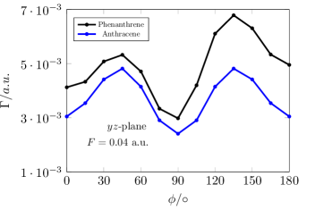
Figure 10: Angle-dependent ionization rates $\Gamma$ of anthracene and phenanthrene (C₁₀H₁₄) in a static electric field of strength $F$=0.04 a.u. computed with RI-MP2. The molecules are in the $xy$ plane while the field is in the $yz$ plane and $\phi$ is the angle between the field and the molecular plane with $\phi=0^{\circ}$ corresponding to the field being parallel to the molecular plane. Reproduced with permission from Ref. 106.

Formally, no changes to Eq. (21) are needed when dealing with CBFs except that the inversion of $\mathbf{J}$ requires care when the auxiliary basis contains CBFs as well. However, the derivation changes: Originally,²⁴⁰ Eq. (21) was obtained by minimizing the functional

$$\Delta_{\mu\nu}=\int dr_{1}\int dr_{2}[\rho_{\mu\nu}(r_{1})-\tilde{\rho}_{\mu\nu}(r_{1})]\,r_{12}^{-1}\,[\rho_{\sigma\rho}(r_{2})-\tilde{\rho}_{\sigma\rho}(r_{2})]$$ (22)

with $\tilde{\rho}_{\mu\nu}$ and $\rho_{\mu\nu}$ as approximated and exact AO products, respectively. This is not possible for a basis set containing CBFs because $\Delta_{\mu\nu}$ becomes complex as well. In Ref. 105 the absolute value $|\Delta_{\mu\nu}|$ was minimized instead, which also led to Eq. (21).

Initial applications¹⁰⁵ of CBF-RI-MP2 employed customized auxiliary basis sets including several complex-scaled shells, but it was later demonstrated¹⁰⁶ that real-valued auxiliary basis sets optimized for standard RI-MP2 calculations work equally well. As a result, typical CBF-RI-MP2 calculations employ auxiliary basis sets that have roughly the same size as the original basis set. This is different from standard RI-MP2, where one usually uses considerably larger auxiliary basis sets.

Very recently, Eq. (21) has been made available for use in CC2 calculations with CBFs.²⁵⁵ As a multistate method, CC2 in its EOM extension can provide a description of a resonance together with its decay channels and is thus appropriate for further types of resonances besides ionization in static fields, for example, core-excited states and temporary anions. Since CC2 and MP2 are structurally similar,^{201, 202} it is expected that complex-variable RI-CC2 will be applicable to resonances in systems with up to ca. 50 atoms as well. In addition, the RI approximation has been made available for CAP-MP2 and CAP-CC2 calculations. Since CAP methods are based on real-valued AOs, the usual RI approximation can be used and the $B$ tensors from Eq. (21) become complex only upon transformation to the MO basis.

It should be added that it is also possible to apply Eq. (21) to the ERIs in the context of CCSD and EOM-CCSD.²⁵⁶ However, this reduces computation times and memory requirements much less than in the case of MP2 or CC2 because the amplitudes $t_{ij}^{ab}$ need to be stored and processed in every iteration. Given that the treatment of resonances often requires large basis sets, computational savings could be potentially higher than for bound states and complex-variable RI-CCSD may thus be a more viable method than its real-valued counterpart. However, no implementation has been reported so far.

4.3 Quantum embedding

To investigate electronic resonances in complex environments, a possible further strategy besides the use of rank-reduction techniques consists in wave-function-theory in DFT quantum embedding.^{257, 258} Here, only a small region of interest in a larger system is treated with a high-level method, for example EOM-CC, whereas the remainder is described using a lower-cost DFT approximation. Since embedding approaches rely on partitioning the system, they are particularly useful whenever the fragment of interest and the environment can be told apart easily, for example, if one deals with molecules that are surrounded by a solvation shell, absorbed at a surface, or enclosed in a protein coat.

While there are many investigations where quantum embedding is used to describe properties and chemical reactivity of electronic ground states, applications to excitation, ionization, and electron attachment are a lot scarcer.²⁴⁹ A central question is whether it is appropriate to use the same embedding potential for different electronic states. Recently, it was shown that a state-universal approach based on projection-based EOM-CCSD-in-DFT embedding^{259, 260, 261} delivers good numerical results for excited states of valence, Rydberg, and charge-transfer character, for valence and core ionization, and with certain reservations, also for electron-attached states.²⁶² Through combination with CAPs and CBFs, the method has been extended to electronic resonances.²⁶²

As an illustration of the numerical performance, Tab. 1 lists representative results for several types of transitions computed with embedded and regular EOM-CCSD as well as with DFT. In all these examples, the environment, which is treated with DFT, consists of 1–5 water molecules simulating microsolvation. Although it can be seen that valence excitation energies and valence ionization energies are well described by embedded EOM-CCSD, the usefulness of the approach for these transition is questionable given the good performance of DFT, represented in Tab. 1 by the Coulomb-attenuated B3LYP density functional. More interesting are thus applications to core ionization and Rydberg excited states, where DFT struggles while embedded EOM-CCSD performs well. As concerns electron attachment, Tab. 1 demonstrates that embedded EOM-CCSD improves on DFT but –because attachment energies are typically very small– the deviation from regular EOM-CCSD is still larger than the actual transition energy. However, for positive attachment energies corresponding to temporary attachment, which can be larger, the performance of embedded CAP-EOM-CCSD is satisfying both for the real part of the energy and the imaginary part corresponding to the decay width.

Table 1:  Different types of transition energies computed with regular and embedded EOM-CCSD. Absolute values are given for regular EOM-CCSD, deviations from these values for embedded EOM-CCSD. All values are in eV and have been taken from Ref. 262

Type of state	Example	EOM-CCSD	EOM-CCSD embedded in		CAM-B3LYP
			CAM-B3LYP	PBE
Valence excitation	CH2O + 5 H2O	4.08	0.05	0.04	–0.06
Rydberg excitation	CH3OH + 3 H2O	8.75	–0.03	–0.48	–0.68
Valence ionization	CH2O + 5 H2O	11.19	0.12	0.10	–0.15
Core ionization	CH2O + 5 H2O	540.95	0.06	0.04	–1.40
Electron attachment	HCF + 5 H2O	–0.07	–0.48	–1.49	–1.40
Temporary electron attachment	CH2O + H2O	0.88–0.10$i$	—	0.91–0.11$i$	—

For the projection-based embedded EOM-CCSD method employed in Tab. 1, one first solves a standard SCF equation for the whole system, denoted A+B, using a suitable density functional. Based on localization of the orbitals and Mulliken population analysis, the resulting SCF wave function is then split into two pieces corresponding to the high-level fragment A and the environment B. Subsequently, a second SCF procedure is carried out with a modified Fock matrix $\tilde{\mathbf{F}}$, whose elements are given as

$$\tilde{F}^{\text{A-in-B}}_{\kappa\lambda} =\sum_{\sigma\rho}\mathcal{P}_{\kappa\mu}F^{\text{A-in-B}}_{\mu\nu}\mathcal{P}_{\nu\lambda}~{},$$ (23)

$$F^{\text{A-in-B}}_{\mu\nu} =h_{\mu\nu}+\sum_{\rho\sigma}\gamma^{\text{A-in-B}}_{\sigma\rho}[\langle\mu\sigma|\nu\rho\rangle-\langle\mu\sigma|\rho\nu\rangle]+v^{\text{emb}}_{\mu\nu}~{}.$$ (24)

This determines the density matrix $\boldsymbol{\gamma}^{\text{A-in-B}}$ that forms the basis for the subsequent CCSD and EOM-CCSD calculations. In Eq. (24), the embedding potential is given as $v^{\text{emb}}_{\mu\nu}=\sum_{\sigma\rho}[\gamma^{\text{A+B}}_{\sigma\rho}-\gamma^{\text{A}}_{\sigma\rho}]\,[\langle\mu\sigma|\nu\rho\rangle-\langle\mu\sigma|\rho\nu\rangle]$ and thus independent of $\boldsymbol{\gamma}^{\text{A-in-B}}$ so that it does not need to be recalculated during the SCF procedure. The projector $\mathcal{P}_{\mu\nu}=\delta_{\mu\nu}-\sum_{\rho}\gamma^{\text{B}}_{\mu\rho}\;S_{\rho\nu}$ removes the degrees of freedom corresponding to subsystem B from the variational space. This formulation of the theory in terms of Eqs. (23) and (24) is equivalent to the one originally introduced.²⁵⁹

Eqs. (23) and (24) ensure that the SCF energy of the full system A+B is recovered exactly if both fragments are described at the same level of theory.^{259, 260} A further advantage of projection-based embedding is that no modifications are necessary to the working equations of the higher-level method as long as one is only interested in the energy or orbital-unrelaxed properties. Likewise, quantities such as NTOs and Dyson orbitals that are useful to characterize excitation, ionization or electron attachment, can be evaluated in a straightforward manner.²⁶² The fact that the working equations of the higher-level method stay the same is also the reason that the combination of projection-based embedding with CAP-EOM-CCSD is very easy if the CAP is active only in the EOM-CCSD calculation. In such an approach, the SCF calculation based on Eqs. (23) and (24) stays real-valued. The combination with CBFs is conceptually simple as well but requires the implementation of Eqs. (23) and (24) for complex numbers.

4.4 Partial decay widths

Most electronic resonances can decay into different electronic states, which are referred to as decay channels. For example, metastable excited states of CN^- can decay into the ${}^{2}\Sigma^{+}$ and the ${}^{2}\Pi$ state of neutral CN.²⁰⁸ A core-ionized H₂O molecule with electronic configuration $(1a_{1})^{1}(2a_{1})^{2}(1b_{2})^{2}(3a_{1})^{2}(1b_{1})^{2}$ can decay into 16 states of H₂O²⁺ where shake-up processes and double Auger decay have not even been considered yet.^{263, 136} In a molecule exposed to a static electric field, electrons from all orbitals can undergo tunnel ionization giving rise to a multitude of decay channels but the relative ease with which ionization from a particular orbital happens greatly depends on the orientation of the field and the molecule.^{104, 106}

Partial decay widths describing the contributions of different channels are thus of great importance for the chemistry and physics of electronic resonances. The notable exception are low-lying temporary radical anions formed by electron attachment to closed-shell molecules, which typically decay solely into their parent state meaning the neutral ground state. For all other types of resonances, partial widths are central quantities to analyze the fate of a metastable system. In addition, branching ratios can often be determined experimentally with much better accuracy than total decay widths.

However, while there are ample theoretical data on partial decay widths of atomic resonances and those in diatomic or triatomic molecules, corresponding investigations of polyatomic molecules are comparatively scarce.^{264, 46, 265, 266, 267, 47, 43, 48, 263, 136} Most computations relied on Fano’s theory^{40, 41} where the determination of partial widths is straightforward because the total width is obtained as a sum over decay channels. This is not the case for complex-variable methods, where the total decay width is evaluated according to Eq. (1), i.e., as imaginary part of an eigenvalue of the Schrödinger equation. Consequently, additional steps have to be taken to define partial decay widths and very few data are available so far.

In some cases, the evaluation of partial widths with complex-variable methods is facilitated by point-group symmetry. For example, the CAP-MRCI decay width of C${}_{2}^{2-}$ has been decomposed into contributions from $\sigma_{g}$, $\sigma_{u}$, and $\pi_{u}$ decay channels by projecting the CAP onto orbitals of a particular point-group symmetry.²⁶⁸ In a related manner, the Auger decay width of Ne⁺ (1s^-1) computed with CBF-CCSD has been decomposed into contributions from Ne²⁺ states of S, P, or D symmetry by complex scaling only s, p, or d shells of the basis set, respectively.¹³⁶ It has also been suggested to decompose the total width obtained in a CAP calculation using Fano’s theory by considering the overlap between a Dyson orbital and a Coulomb wave representing the free electron²¹¹ or, alternatively, by analyzing NTOs.²⁰⁸ These approaches were applied to C${}_{2}^{2-}$ and cyanopolyyne anions using CCSD and EOM-EA-CCSD wave functions, respectively.

Recently, a more general approach was introduced to evaluate partial widths in the context of complex-variable methods.¹³⁶ This approach is independent of point-group symmetry and does not make use of Fano’s theory. Instead, it is based on energy decomposition analysis. In initial applications, it was applied to Auger decay of core-ionized states described with CS-CCSD and CBF-CCSD: For a CC wave function describing a core-ionized state, the decay width stems solely from the imaginary part of the correlation energy

$$E_{\text{CC}}=\sum_{ijab}\Big{(}1/4t_{ij}^{ab}+1/2t_{i}^{a}t_{j}^{b}\Big{)}\langle ij||ab\rangle~{},$$ (25)

because the underlying HF reference does not capture the coupling to the continuum. It is thus possible to assign amplitudes $t_{ij}^{ab}$, in which $a$ or $b$ refer to the core hole, to a particular decay channel depending on the vacated orbitals $i$ and $j$ and to evaluate the partial decay width as contribution of the respective $t_{ij}^{ab}$ to $\text{Im}(E)$. If all amplitudes of this type are removed, a CVS-like wave function is obtained and Eq. (25) yields zero for the imaginary part of the CC energy. As an alternative, the decomposition can be based on the CC Lagrangian

$$E_{\text{CC}}=\langle 0|(1+\Lambda)e^{-T}He^{T}|0\rangle~{},$$ (26)

which yields slightly different results. As a numerical example of the approach, Tab. 2 displays partial decay width of the 16 primary decay channels of core-ionized water computed with CBF-CCSD and, alternatively, based on Fano’s theory. This shows overall good agreement between the methods with the notable exception of the $2a_{1}2a_{1}$ channel, presumably because it has a significant admixture of other states.

While energy expressions corresponding to other wave functions can be analyzed in a likewise manner, the numerical performance of the approach varies. Specifically, the decomposition of the EOMIP-CCSD energy in terms of $R_{2}$ and $L_{2}$ amplitudes yields much less reliable results because excitations that do not result in filling the core hole deliver unphysically large contributions to $\text{Im}(E)$. Likely, it is necessary in this case to analyze further components of the wave functions besides those created by $R_{2}$ and $L_{2}$. A further complication originates from $\text{Im}(E)$ not being exactly zero for bound states in finite basis sets. This is especially pronounced for CS approaches (see Sec. 3.3) but does not impair the performance of the approach too much as Tab. 2 illustrates.

Importantly, Eqs. (25) and (26) apply to all complex-variable methods and types of resonances. The generalization from Auger decay to other processes involving core vacancies as well as to temporary anions and quasistatic ionization, possibly using other wave functions, is thus expected to be straightforward.

Table 2:  Partial decay widths of H₂O⁺ (1s^-1) computed with different methods. All values in meV.

Decay	CBF	Fano	Fano
channel	CCSD136	EOM-CCSD263	MRCI47, 269
$3\text{a}_{1}1\text{b}_{1}$ (triplet)	0.2	0.5	0.4
$1\text{b}_{1}1\text{b}_{1}$	18.0	13.3	19.0
$3\text{a}_{1}1\text{b}_{1}$ (singlet)	19.6	12.7	18.0
$1\text{b}_{1}1\text{b}_{2}$ (triplet)	0	0	0
$3\text{a}_{1}3\text{a}_{1}$	12.2	8.9	13.1
$1\text{b}_{1}1\text{b}_{2}$ (singlet)	15.7	10.7	15.2
$3\text{a}_{1}1\text{b}_{2}$ (triplet)	0.2	0.4	0.3
$3\text{a}_{1}1\text{b}_{2}$ (singlet)	13.4	9.5	13.2
$1\text{b}_{2}1\text{b}_{2}$	8.7	7.1	9.8
$2\text{a}_{1}1\text{b}_{1}$ (triplet)	2.8	4.1	3.0
$2\text{a}_{1}3\text{a}_{1}$ (triplet)	2.5	3.8	2.6
$2\text{a}_{1}1\text{b}_{2}$ (triplet)	2.2	2.9	1.6
$2\text{a}_{1}1\text{b}_{1}$ (singlet)	9.6	9.5	10.0
$2\text{a}_{1}3\text{a}_{1}$ (singlet)	12.7	13.6	11.0
$2\text{a}_{1}1\text{b}_{2}$ (singlet)	6.8	6.3	6.6
$2\text{a}_{1}2\text{a}_{1}$	21.6	15.3	4.1
All	142.5	121.7	145.6

5 Conclusions and outlook

This feature article has given an overview of the quantum chemistry of electronic resonances and their treatment by means of complex-variable electronic-structure methods. Because resonances are embedded in the continuum, their wave functions are a priori not square-integrable. Complex-variable techniques afford a regularization of resonances and make them amenable to bound-state quantum chemistry. Quantities such as Dyson orbitals and natural transition orbitals can be defined and an analysis of resonances in terms of molecular orbital theory becomes possible.

Regularization of resonance wave functions can be achieved by means of complex scaling or complex absorbing potentials. While complex scaling offers several formal advantages and can now be applied to molecular resonances without problems using complex-scaled basis functions, complex absorbing potentials are more heuristic but also easier to integrate into existing software. In addition, CAP calculations can be sped up by activating the CAP only in certain steps of a calculation. However, the unphysical dependence of the complex resonance energy on parameters such as scaling angle and CAP strength presents a persistent stumbling block shared by CAP and complex-scaled approaches.

Different types of resonances, in particular temporary anions, core-vacant states, and Stark resonances were discussed with respect to their electronic structure and their decay mechanism. These states pose distinct requirements towards the electronic-structure model. For temporary anions, superexcited states, core-excited and core-vacant states, a multistate treatment as offered by EOM-CC, SAC-CI, CC2, or ADC methods combines several advantages. For other states such as metastable dianions, the identification of the most suitable computational approach is less straightforward. The feature article has furthermore summarized a number of recent methodological contributions to the field:

• The development of analytic gradients for CAP-CC methods has enabled the investigation of potential energy surfaces of polyatomic temporary anions. Special points such as equilibrium structures, crossing seams, and exceptional points can be located and characterized; the results demonstrate the relevance of such points for chemical reactions and spectroscopies involving electronic resonances. In addition, the availability of analytic gradients paves the way for conducting ab initio molecular dynamics simulations of decaying states. Such calculations will be most relevant to model DEA efficiencies.

• The development of a resolution-of-the-identity approximation for complex basis functions has enabled the treatment of resonances in molecules with up to ca. 50 atoms at the MP2 level of theory. Because resonances require large basis sets with many diffuse functions, substantial speedups can be achieved by means of the RI approximation. Notably, standard auxiliary bases without any complex-scaled functions deliver excellent results for energies and decay widths. The introduction of RI methods for resonances can be seen as a first step towards the application of further rank-reduction techniques such as Cholesky decomposition.^{242, 244} Moreover, multistate methods such as complex-variable CC2 have very recently been combined with the RI approximation as well; these approaches are expected to benefit from similar advantages as MP2.

• Projection-based wave-function-theory in density-functional-theory embedding provides a way to quantify the impact of the chemical environment on a resonance state. The method has so far only been used for microsolvated temporary anions described by CAP-EOM-CCSD, where is delivers good results for energies and decay widths. A corresponding approach based on complex basis functions that is geared towards core-vacant states has very recently been achieved as well. Most interesting in this context will be applications to decay processes such as interatomic Coulombic decay that occur only through participation of the environment.

• Partial decay widths have been made available by means of an energy decomposition analysis that is related to the core-valence separation. The method has been applied to Auger decay of core-ionized states described by complex basis functions and EOM-CCSD, but can be generalized to other wave functions and kinds of resonances. Partial widths are critically important for all states for which more than one decay channel is open including different types of superexcited, core-vacant, and Stark resonances.

The present feature article illustrates that complex-variable techniques and, more general, quantum chemistry of electronic resonances is a field of active research. The developments introduced in recent years have broadened the scope of electronic-structure theory significantly and enabled new types of applications in computational chemistry and spectroscopy. Although there remain formal as well as technical issues to be solved, the implementations of complex scaling and complex absorbing potentials that are available today already represent a useful enhancement of quantum chemistry. Further research on complex-variable techniques is underway and provides the perspective of making these methods more practical so that, ultimately, they may be routinely used by non-experts as tool in quantum-chemistry program packages.

Conflicts of interest

There are no conflicts to declare.

References

- Gamov 1928 G. Gamov, Z. Phys., 1928, 51, 204–212.
- Myo and Kato 2020 T. Myo and K. Kato, Prog. Theor. Exp. Phys., 2020, 2020, 12A101.
- Hättig 2005 C. Hättig, Adv. Quantum Chem., 2005, 50, 37–60.
- Köhn and Tajti 2007 A. Köhn and A. Tajti, J. Chem. Phys., 2007, 127, 044105.
- Kjønstad and Koch 2017 E. F. Kjønstad and H. Koch, J. Phys. Chem. Lett., 2017, 8, 4801–4807.
- S. Thomas and Gauss 2021 S. S. S. Thomas, F. Hampe and J. Gauss, Mol. Phys., 2021, 119, e1968056.
- Agarwal 2013 B. K. Agarwal, X-ray spectroscopy: an introduction, Springer Verlag, Berlin, Heidelberg, 2013.
- Norman and Dreuw 2018 P. Norman and A. Dreuw, Chem. Rev., 2018, 118, 7208–7248.
- Zimmermann et al. 2020 P. Zimmermann, S. Peredkov, P. M. Abdala, S. DeBeer, M. Tromp, C. Müller and J. A. van Bokhoven, Coord. Chem. Rev., 2020, 423, 213466.
- Simons 2011 J. Simons, Annu. Rev. Phys. Chem., 2011, 62, 107–128.
- Herbert 2015 J. M. Herbert, Rev. Comp. Chem., 2015, 28, 391–517.
- Alizadeh et al. 2015 E. Alizadeh, T. M. Orlando and L. Sanche, Annu. Rev. Phys. Chem., 2015, 66, 379–398.
- Scrinzi et al. 2006 A. Scrinzi, M. Y. Ivanov, R. Kienberger and D. M. Villeneuve, J. Phys. B, 2006, 39, R1–R37.
- Gallmann et al. 2012 L. Gallmann, C. Cirelli and U. Keller, Annu. Rev. Phys. Chem., 2012, 63, 447–469.
- Moiseyev 2011 N. Moiseyev, Non-Hermitian Quantum Mechanics, Cambridge University Press, Cambridge, UK, 2011.
- Reinhardt 1982 W. P. Reinhardt, Annu. Rev. Phys. Chem., 1982, 33, 223–255.
- Jagau et al. 2017 T.-C. Jagau, K. Bravaya and A. I. Krylov, Annu. Rev. Phys. Chem., 2017, 68, 525–553.
- Császár et al. 2020 A. G. Császár, I. Simkó, T. Szidarovszky, G. C. Groenenboom, T. Karman and A. van der Avoird, Phys. Chem. Chem. Phys., 2020, 22, 15081–15104.
- Baer and Neuhauser 2003 R. Baer and D. Neuhauser, Chem. Phys. Lett., 2003, 374, 459–463.
- Ernzerhof 2006 M. Ernzerhof, J. Chem. Phys., 2006, 125, 124104.
- Cederbaum et al. 1980 L. S. Cederbaum, W. Domcke and J. Schirmer, Phys. Rev. A, 1980, 22, 206–222.
- Hazi and Taylor 1970 A. U. Hazi and H. S. Taylor, Phys. Rev. A, 1970, 1, 1109–1120.
- Nestmann and Peyerimhoff 1985 B. Nestmann and S. D. Peyerimhoff, J. Phys. B, 1985, 18, 615–626.
- Mandelshtam et al. 1994 V. A. Mandelshtam, T. R. Ravuri and H. S. Taylor, J. Chem. Phys., 1994, 101, 8792–8799.
- Simons 1981 J. Simons, J. Chem. Phys., 1981, 75, 2465–2467.
- McCurdy and McNutt 1983 C. W. McCurdy and J. F. McNutt, Chem. Phys. Lett., 1983, 94, 306–310.
- Frey and Simons 1986 R. F. Frey and J. Simons, J. Chem. Phys., 1986, 84, 4462–4469.
- Horáček et al. 2010 J. Horáček, P. Mach and J. Urban, Phys. Rev. A, 2010, 82, 032713.
- Horáček et al. 2015 J. Horáček, I. Paidarová and R. Čurík, J. Chem. Phys., 2015, 143, 184102.
- Sommerfeld and Ehara 2015 T. Sommerfeld and M. Ehara, J. Chem. Phys., 2015, 142, 034105.
- Head-Gordon and McCurdy 2017 A. F. W. M. Head-Gordon and C. W. McCurdy, J. Chem. Phys., 2017, 146, 044112.
- Taylor 1972 J. R. Taylor, Scattering Theory: The Quantum Theory on Nonrelativistic Collisions, Wiley, New York, 1972.
- Domcke 1991 W. Domcke, Phys. Rep., 1991, 208, 97–188.
- Tennyson 2010 J. Tennyson, Phys. Rep., 2010, 491, 29–76.
- da Costa et al. 2015 R. F. da Costa, M. T. do N. Varella, M. H. F. Bettega and M. A. Lima, Eur. J. Phys. D, 2015, 69, 159.
- Lane 1980 N. F. Lane, Rev. Mod. Phys., 1980, 52, 29–119.
- Ingólfsson 2019 O. Ingólfsson, Low-Energy Electrons: Fundamentals and Applications, Jenny Stanford Publishing, Singapore, 2019.
- Gorfinkiel 2020 J. D. Gorfinkiel, Eur. J. Phys. D, 2020, 74, 51.
- Mašín et al. 2020 Z. Mašín, J. Benda, J. D. Gorfinkiel, A. G. Harvey and J. Tennyson, Comput. Phys. Commun., 2020, 249, 107092.
- Fano 1961 U. Fano, Phys. Rev., 1961, 124, 1866–1878.
- Feshbach 1962 H. Feshbach, Ann. Phys. (N.Y.), 1962, 19, 287–313.
- Averbukh and Cederbaum 2005 V. Averbukh and L. S. Cederbaum, J. Chem. Phys., 2005, 123, 204107.
- Kolorenč and Averbukh 2020 P. Kolorenč and V. Averbukh, J. Chem. Phys., 2020, 152, 214107.
- Langhoff and Corcoran 1974 P. W. Langhoff and C. T. Corcoran, J. Chem. Phys., 1974, 61, 146–159.
- Carravetta and Ågren 1987 V. Carravetta and H. Ågren, Phys. Rev. A, 1987, 35, 1022–1032.
- Zähringer et al. 1992 K. Zähringer, H.-D. Meyer and L. S. Cederbaum, Phys. Rev. A, 1992, 45, 318–328.
- Inhester et al. 2012 L. Inhester, C. F. Burmeister, G. Groenhof and H. Grubmüller, J. Chem. Phys., 2012, 136, 144304.
- Skomorowski and Krylov 2021 W. Skomorowski and A. I. Krylov, J. Chem. Phys., 2021, 154, 084124.
- Aguilar and Combes 1971 J. Aguilar and J. M. Combes, Commun. Math. Phys., 1971, 22, 269–279.
- Balslev and Combes 1971 E. Balslev and J. M. Combes, Commun. Math. Phys., 1971, 22, 280–294.
- Simon 1972 B. Simon, Commun. Math. Phys., 1972, 27, 1–9.
- Moiseyev 1998 N. Moiseyev, Phys. Rep., 1998, 302, 211–293.
- McCurdy and Rescigno 1978 C. W. McCurdy and T. N. Rescigno, Phys. Rev. Lett., 1978, 41, 1364–1368.
- Moiseyev and Corcoran 1979 N. Moiseyev and C. Corcoran, Phys. Rev. A, 1979, 20, 814–817.
- Jolicard and Austin 1985 G. Jolicard and E. J. Austin, Chem. Phys. Lett., 1985, 121, 106–110.
- Riss and Meyer 1993 U. V. Riss and H.-D. Meyer, J. Phys. B, 1993, 26, 4503–4536.
- Simons 2008 J. Simons, J. Phys. Chem. A, 2008, 112, 6401–6511.
- Fabrikant et al. 2017 I. I. Fabrikant, S. Eden, N. J. Mason and J. Fedor, Adv. At. Mol. Opt. Phys., 2017, 66, 545–657.
- Studer and Curran 2014 A. Studer and D. P. Curran, Nat. Chem., 2014, 6, 765–773.
- Aslam et al. 2018 U. Aslam, V. G. Rao, S. Chavez and S. Linic, Nat. Catal., 2018, 1, 656–665.
- Li et al. 2018 S. Li, J. A. Medrano, V. Hessel and F. Gallucci, Processes, 2018, 6, 248–273.
- Boudaïffa et al. 2000 B. Boudaïffa, P. Cloutier, D. Hunting, M. A. Huels and L. Sanche, Science, 2000, 287, 1658–1660.
- Jagau et al. 2015 T.-C. Jagau, D. B. Dao, N. S. Holtgrewe, A. I. Krylov and R. Mabbs, J. Phys. Chem. Lett., 2015, 6, 2786–2793.
- Lyle et al. 2018 J. Lyle, S. R. Chandramoulee, J. R. Hamilton, B. A. Traylor, T. L. Guasco, T.-C. Jagau and R. Mabbs, J. Chem. Phys., 2018, 149, 084302.
- Lyle et al. 2019 J. Lyle, T.-C. Jagau and R. Mabbs, Faraday Discuss., 2019, 217, 533–546.
- Dreuw and Cederbaum 2002 A. Dreuw and L. S. Cederbaum, Chem. Rev., 2002, 102, 181–200.
- Bravaya et al. 2013 K. B. Bravaya, D. Zuev, E. Epifanovsky and A. I. Krylov, J. Chem. Phys., 2013, 138, 124106.
- Jagau and Krylov 2016 T.-C. Jagau and A. I. Krylov, J. Chem. Phys., 2016, 144, 054113.
- Jagau 2020 T.-C. Jagau, Nachr. Chem., 2020, 68, 50–54.
- Meitner 1922 L. Meitner, Z. Phys., 1922, 35.
- Auger 1923 P. Auger, CR Acad. Sci. (F), 1923, 177, 169.
- Brown et al. 1980 G. S. Brown, M. H. Chen, B. Crasemann and G. E. Ice, Phys. Rev. Lett., 1980, 45, 1937–1940.
- Piancastelli et al. 1987 M. N. Piancastelli, D. W. Lindle, T. A. Ferrett and D. A. Shirley, J. Chem. Phys., 1987, 86, 2765–2771.
- Kempgens et al. 1999 B. Kempgens, H. M. Köppe, A. Kivimäki, M. Neeb, K. Maier, U. Hergenhahn and A. M. Bradshaw, Surf. Sci., 1999, 425, L376–L380.
- Armen et al. 2000 G. B. Armen, H. Aksela, T. Åberg and S. Aksela, J. Phys. B-At. Mol. Opt., 2000, 33, R49–R92.
- Carlson and Krause 1965 T. A. Carlson and M. O. Krause, Phys. Rev. Lett., 1965, 14, 390–392.
- Körber and Mehlhorn 1966 H. Körber and W. Mehlhorn, Z. Phys., 1966, 191, 217–230.
- M. Hotokka and Aksela 1984 H. A. M. Hotokka, H Ågren and S. Aksela, Phys. Rev. A, 1984, 30, 1855–1859.
- Colle and Simonucci 1990 R. Colle and S. Simonucci, Phys. Rev. A, 1990, 42, 3913–3925.
- Coriani and Koch 2015 S. Coriani and H. Koch, J. Chem. Phys., 2015, 143, 181103.
- Zheng and Cheng 2019 X. Zheng and L. Cheng, J. Chem. Theory Comput., 2019, 15, 4945–4955.
- Vidal et al. 2019 M. L. Vidal, X. Feng, E. Epifanovsky, A. I. Krylov and S. Coriani, J. Chem. Theory Comput., 2019, 15, 3117–3133.
- Cederbaum et al. 1997 L. S. Cederbaum, J. Zobeley and F. Tarantelli, Phys. Rev. Lett., 1997, 79, 4778–4781.
- Zobeley et al. 2001 J. Zobeley, R. Santra and L. S. Cederbaum, J. Chem. Phys., 2001, 115, 5076–5088.
- Gokhberg and Cederbaum 2009 K. Gokhberg and L. S. Cederbaum, J. Phys. B, 2009, 42, 231001.
- Jahnke et al. 2020 T. Jahnke, U. Hergenhahn, B. Winter, R. Dörner, U. Frühling, P. V. Demekhin, K. Gokhberg, L. S. Cederbaum, A. Ehresmann, A. Knie and A. Dreuw, Chem. Rev., 2020, 120, 11295–11369.
- Ouchi et al. 2011 T. Ouchi, K. Sakai, H. Fukuzawa, X.-J. Liu, I. Higuchi, Y. Tamenori, K. Nagaya, H. Iwayama, M. Yao, D. Zhang, D. Ding, A. I. Kuleff, S. D. Stoychev, P. V. Demekhin, N. Saito and K. Ueda, Phys. Rev. Lett., 2011, 107, 053401.
- Scrinzi et al. 1999 A. Scrinzi, M. Geissler and T. Brabec, Phys. Rev. Lett., 1999, 83, 706–709.
- Herbst 1979 I. W. Herbst, Commun. Math. Phys., 1979, 64, 279–298.
- Herbst and Simon 1981 I. W. Herbst and B. Simon, Commun. Math. Phys., 1981, 80, 181–216.
- Caliceti et al. 2007 E. Caliceti, M. Meyer-Hermann, P. Ribeca, A. Surzhykov and U. D. Jentschura, Phys. Rep., 2007, 446, 1–96.
- Jagau 2016 T.-C. Jagau, J. Chem. Phys., 2016, 145, 204115.
- Helgaker et al. 2012 T. Helgaker, S. Coriani, P. Jørgensen, K. Kristensen, J. Olsen and K. Ruud, Chem. Rev., 2012, 112, 543–631.
- Reiss 2008 H. R. Reiss, Phys. Rev. Lett., 2008, 101, 043002.
- Keldysh 1965 L. V. Keldysh, Sov. Phys. JETP, 1965, 20, 1307–1314.
- Oppenheimer 1928 J. R. Oppenheimer, Phys. Rev., 1928, 13, 66–81.
- Landau and Lifschitz 1977 L. D. Landau and E. M. Lifschitz, Quantum Mechanics: Non-Relativistic Theory, Pergamon Press, Oxford, New York, 1977.
- Yamabe et al. 1977 T. Yamabe, A. Tachibana and H. J. Silverstone, Phys. Rev. A, 1977, 16, 877–890.
- Ammosov et al. 1986 M. V. Ammosov, N. B. Delone and V. P. Krainov, Sov. Phys. JETP, 1986, 64, 1191–1194.
- Tong et al. 2002 X. M. Tong, Z. X. Zhao and C. D. Lin, Phys. Rev. A, 2002, 66, 033402.
- Batishchev et al. 2010 P. A. Batishchev, O. I. Tolstikhin and T. Morishita, Phys. Rev. A, 2010, 82, 023416.
- Tolstikhin et al. 2014 O. I. Tolstikhin, L. B. Madsen and T. Morishita, Phys. Rev. A, 2014, 89, 013421.
- Yue et al. 2017 L. Yue, S. Bauch and L. B. Madsen, Phys. Rev. A, 2017, 96, 043408.
- Jagau 2018 T.-C. Jagau, J. Chem. Phys., 2018, 148, 204102.
- Hernández Vera and Jagau 2019 M. Hernández Vera and T.-C. Jagau, J. Chem. Phys., 2019, 151, 111101.
- Hernández Vera and Jagau 2020 M. Hernández Vera and T.-C. Jagau, J. Chem. Phys., 2020, 152, 174103.
- Platzman 1962 R. L. Platzman, Radiat. Res., 1962, 17, 419–425.
- Hatano 2003 Y. Hatano, Radiat. Phys. Chem., 2003, 67, 183–198.
- Reinhardt 1976 W. P. Reinhardt, Int. J. Quantum Chem., 1976, 10, 359–367.
- Majety and Scrinzi 2015 V. P. Majety and A. Scrinzi, J. Phys. B, 2015, 48, 245603.
- Schulz 1973 G. J. Schulz, Rev. Mod. Phys., 1973, 45, 423–486.
- Ibǎnescu et al. 2007 B. C. Ibǎnescu, O. May, A. Monney and M. Allan, Phys. Chem. Chem. Phys., 2007, 9, 3163–3173.
- Ibǎnescu and Allan 2008 B. C. Ibǎnescu and M. Allan, Phys. Chem. Chem. Phys., 2008, 10, 5232–5237.
- Klinker et al. 2018 M. Klinker, C. Marante, L. Argenti, J. González-Vázquez and F. Martín, J. Phys. Chem. Lett., 2018, 9, 756–762.
- Plunkett et al. 2019 A. Plunkett, N. Harkema, R. R. Lucchese, C. W. McCurdy and A. Sandhu, Phys. Rev. A, 2019, 99, 063403.
- Rabadán and Gorfinkiel 2021 I. Rabadán and J. D. Gorfinkiel, Phys. Rev. A, 2021, 103, 032804.
- Sommerfeld and Cederbaum 1998 T. Sommerfeld and L. S. Cederbaum, Phys. Rev. Lett., 1998, 80, 3723–3726.
- Dreuw and Cederbaum 1999 A. Dreuw and L. S. Cederbaum, Phys. Rev. A, 1999, 59, 2702–2706.
- Dreuw and Cederbaum 1999 A. Dreuw and L. S. Cederbaum, J. Phys. B, 1999, 32, L665–L672.
- Dreuw and Cederbaum 1999 A. Dreuw and L. S. Cederbaum, Int. J. Mass Spectrom., 1999, 188, 199–204.
- Siegert 1939 A. J. F. Siegert, Phys. Rev., 1939, 56, 750–752.
- Meyer and Walter 1982 H.-D. Meyer and O. Walter, J. Phys. B, 1982, 15, 3647–3668.
- Moiseyev et al. 1978 N. Moiseyev, P. R. Certain and F. Weinhold, Mol. Phys., 1978, 36, 1613–1630.
- Brändas and Froelich 1977 E. Brändas and P. Froelich, Phys. Rev. A, 1977, 16, 2207–2210.
- Moiseyev 1982 N. Moiseyev, Mol. Phys., 1982, 47, 585–598.
- Reed and Simon 1982 M. Reed and B. Simon, Methods of Modern Mathematical Physics, Volume IV, Academic, New York, 1982.
- Löwdin 1988 P.-O. Löwdin, Adv. Quantum Chem., 1988, 19, 87–138.
- Löwdin et al. 1989 P.-O. Löwdin, P. Froelich and M. Mishra, Adv. Quantum Chem., 1989, 20, 185–237.
- Herbst and Simon 1978 I. W. Herbst and B. Simon, Phys. Rev. Lett., 1978, 41, 67–69.
- Nicolaides and Themelis 1992 C. A. Nicolaides and S. I. Themelis, Phys. Rev. A, 1992, 45, 349–357.
- McCurdy et al. 1991 C. W. McCurdy, C. K. Stroud and M. K. Wisinski, Phys. Rev. A, 1991, 43, 5980–5990.
- Scrinzi and Elander 1993 A. Scrinzi and N. Elander, J. Chem. Phys., 1993, 98, 3866–3875.
- Rescigno and McCurdy 2000 T. N. Rescigno and C. W. McCurdy, Phys. Rev. A, 2000, 62, 032706.
- Rescigno et al. 2005 T. N. Rescigno, D. A. Horner, F. L. Yip and C. W. Mcurdy, Phys. Rev. A, 2005, 72, 052709.
- Chuljian and Simons 1983 D. T. Chuljian and J. Simons, Int. J. Quantum Chem, 1983, 23, 1723–1738.
- Matz and Jagau 2021 F. Matz and T.-C. Jagau, J. Chem. Phys., 2021, submitted.
- Venkatnathan et al. 2000 A. Venkatnathan, M. K. Mishra and H. J. A. Jensen, Theor. Chim. Acta, 2000, 104, 445–454.
- Ždánská and Moiseyev 2005 P. R. Ždánská and N. Moiseyev, J. Chem. Phys., 2005, 123, 194105.
- Kaprálová-Ždánská and Šmydke 2013 P. R. Kaprálová-Ždánská and J. Šmydke, J. Chem. Phys., 2013, 138, 024105.
- Simon 1979 B. Simon, Phys. Lett., 1979, 71 A, 211–214.
- Moiseyev and Hirschfelder 1988 N. Moiseyev and J. O. Hirschfelder, J. Chem. Phys., 1988, 88, 1063–1065.
- Rom et al. 1990 N. Rom, E. Engdahl and N. Moiseyev, J. Chem. Phys., 1990, 93, 3413–3419.
- McCurdy and Martín 2004 C. W. McCurdy and F. Martín, J. Phys. B, 2004, 37, 917–936.
- Scrinzi 2010 A. Scrinzi, Phys. Rev. A, 2010, 81, 053845.
- Tao et al. 2009 L. Tao, W. Vanroose, B. Reps, T. N. Rescigno and C. W. McCurdy, Phys. Rev. A, 2009, 80, 063419.
- Yip et al. 2008 F. L. Yip, C. W. McCurdy and T. N. Rescigno, Phys. Rev. A, 2008, 78, 023405.
- Yip et al. 2014 F. L. Yip, C. W. McCurdy and T. N. Rescigno, Phys. Rev. A, 2014, 90, 063421.
- Majety et al. 2015 V. P. Majety, A. Zielinksi and A. Scrinzi, New J. Phys., 2015, 17, 063002.
- Orimo et al. 2018 Y. Orimo, T. Sato, A. Scrinzi and K. L. Ishikawa, Phys. Rev. A, 2018, 97, 023423.
- Rescigno et al. 1980 T. N. Rescigno, A. E. Orel and C. W. McCurdy, J. Chem. Phys., 1980, 73, 6347–6348.
- McCurdy et al. 1980 C. W. McCurdy, T. N. Rescigno, E. R. Davidson and J. G. Lauderdale, J. Chem. Phys., 1980, 73, 3268.
- Honigmann et al. 1999 M. Honigmann, G. Hirsch, R. J. Buenker, I. D. Petsalakis and G. Theodorakopoulos, Chem. Phys. Lett., 1999, 305, 465–473.
- Honigmann et al. 2006 M. Honigmann, R. J. Buenker and H.-P. Liebermann, J. Chem. Phys., 2006, 125, 234304.
- Honigmann et al. 2010 M. Honigmann, H.-P. Liebermann and R. J. Buenker, J. Chem. Phys., 2010, 133, 044305.
- White et al. 2015 A. F. White, M. Head-Gordon and C. W. McCurdy, J. Chem. Phys., 2015, 142, 054103.
- White et al. 2015 A. F. White, C. W. McCurdy and M. Head-Gordon, J. Chem. Phys., 2015, 143, 074103.
- White et al. 2017 A. F. White, E. Epifanovsky and C. W. McCurdy, J. Chem. Phys., 2017, 146, 234107.
- Muga et al. 2004 J. G. Muga, J. Palao, B. Navarro and I. L. Egusquiza, Phys. Rep., 2004, 395, 357–426.
- Riss and Meyer 1995 U. V. Riss and H.-D. Meyer, J. Phys. B, 1995, 28, 1475–1493.
- Riss and Meyer 1998 U. V. Riss and H.-D. Meyer, J. Phys. B, 1998, 31, 2279–2304.
- Moiseyev 1998 N. Moiseyev, J. Phys. B, 1998, 31, 1431–1441.
- Zuev et al. 2014 D. Zuev, T.-C. Jagau, K. B. Bravaya, E. Epifanovsky, Y. Shao, E. Sundstrom, M. Head-Gordon and A. I. Krylov, J. Chem. Phys., 2014, 141, 024102.
- Rom et al. 1991 N. Rom, N. Lipkin and N. Moiseyev, Chem. Phys., 1991, 151, 199–204.
- Sajeev et al. 2006 Y. Sajeev, M. Sindelka and N. Moiseyev, Chem. Phys., 2006, 329, 307–312.
- Sommerfeld and Santra 2001 T. Sommerfeld and R. Santra, Int. J. Quantum Chem., 2001, 82, 218–226.
- Ghosh et al. 2012 A. Ghosh, N. Vaval and S. Pal, J. Chem. Phys., 2012, 136, 234110.
- Sommerfeld and Ehara 2015 T. Sommerfeld and M. Ehara, J. Chem. Theory Comput., 2015, 11, 4627–4633.
- Sommerfeld et al. 1998 T. Sommerfeld, U. V. Riss, H.-D. Meyer, L. S. Cederbaum, B. Engels and H.-U. Suter, J. Phys. B, 1998, 31, 4107–4122.
- Santra 2006 R. Santra, Phys. Rev. A, 2006, 74, 034701.
- Zuev et al. 2015 D. Zuev, T.-C. Jagau, K. B. Bravaya, E. Epifanovsky, Y. Shao, E. Sundstrom, M. Head-Gordon and A. I. Krylov, J. Chem. Phys., 2015, 143, 149901.
- Jagau et al. 2014 T.-C. Jagau, D. Zuev, K. B. Bravaya, E. Epifanovsky and A. I. Krylov, J. Phys. Chem. Lett., 2014, 5, 310–314.
- Jagau et al. 2015 T.-C. Jagau, D. Zuev, K. B. Bravaya, E. Epifanovsky and A. I. Krylov, J. Phys. Chem. Lett., 2015, 6, 3866.
- Ehara et al. 2016 M. Ehara, R. Fukuda and T. Sommerfeld, J. Comp. Chem., 2016, 37, 242–249.
- Benda and Jagau 2017 Z. Benda and T.-C. Jagau, J. Chem. Phys., 2017, 146, 031101.
- Benda and Jagau 2018 Z. Benda and T.-C. Jagau, J. Chem. Theory Comput., 2018, 14, 3468–3478.
- Santra and Cederbaum 2001 R. Santra and L. S. Cederbaum, J. Chem. Phys., 2001, 115, 6853–6861.
- Lefebvre et al. 2005 R. Lefebvre, M. Sindelka and N. Moiseyev, Phys. Rev. A, 2005, 72, 052704.
- Landau and Moiseyev 2016 A. Landau and N. Moiseyev, J. Chem. Phys., 2016, 145, 164111.
- Landau and Haritan 2019 A. Landau and I. Haritan, J. Phys. Chem. A, 2019, 123, 5091–5105.
- Kunitsa and Bravaya 2019 A. A. Kunitsa and K. B. Bravaya, 2019, https://arxiv.org/abs/1906.11390.
- Whitenack and Wasserman 2011 D. L. Whitenack and A. Wasserman, Phys. Rev. Lett., 2011, 107, 163002.
- Whitenack and Wasserman 2012 D. L. Whitenack and A. Wasserman, J. Chem. Phys., 2012, 136, 164106.
- Zhou and Ernzerhof 2012 Y. Zhou and M. Ernzerhof, J. Phys. Chem. Lett., 2012, 3, 1916–1920.
- Kunitsa et al. 2017 A. A. Kunitsa, A. A. Granovsky and K. B. Bravaya, J. Chem. Phys., 2017, 146, 184107.
- Santra and Cederbaum 2002 R. Santra and L. S. Cederbaum, J. Chem. Phys., 2002, 117, 5511–5521.
- Feuerbacher et al. 2003 S. Feuerbacher, T. Sommerfeld, R. Santra and L. S. Cederbaum, J. Chem. Phys., 2003, 118, 6188–6199.
- Belogolova et al. 2021 A. M. Belogolova, A. L. Dempwolff, A. Dreuw and A. B. Trofimov, J. Phys. Conf. Ser., 2021, 1847, 012050.
- Dempwolff et al. 2021 A. L. Dempwolff, A. M. Belogolova, T. Sommerfeld, A. B. Trofimov and A. Dreuw, J. Chem. Phys., 2021, 155, 054103.
- Ehara and Sommerfeld 2012 M. Ehara and T. Sommerfeld, Chem. Phys. Lett., 2012, 537, 107–112.
- Sajeev et al. 2005 Y. Sajeev, R. Santra and S. Pal, J. Chem. Phys., 2005, 122, 234320.
- Jagau and Krylov 2014 T.-C. Jagau and A. I. Krylov, J. Phys. Chem. Lett., 2014, 5, 3078–3085.
- Shavitt and Bartlett 2009 I. Shavitt and R. J. Bartlett, Many-Body Methods in Chemistry and Physics: MBPT and Coupled-Cluster Theory, Cambridge University Press, 2009.
- Krylov 2008 A. I. Krylov, Annu. Rev. Phys. Chem., 2008, 59, 433–462.
- Sneskov and Christiansen 2012 K. Sneskov and O. Christiansen, WIREs Comput. Mol.Sci., 2012, 2, 566–584.
- Bartlett 2012 R. J. Bartlett, WIREs Comput. Mol. Sci., 2012, 2, 126–138.
- Emrich 1981 K. Emrich, Nucl. Phys. A, 1981, 351, 379–396.
- Sekino and Bartlett 1984 H. Sekino and R. J. Bartlett, Int. J. Quantum Chem., 1984, 26, 255–265.
- Stanton and Bartlett 1993 J. F. Stanton and R. J. Bartlett, J. Chem. Phys., 1993, 98, 7029–7039.
- Nooijen and Snijders 1993 M. Nooijen and J. G. Snijders, Int. J. Quantum Chem., 1993, 48, 15–48.
- Stanton and Gauss 1994 J. F. Stanton and J. Gauss, J. Chem. Phys., 1994, 101, 8938–8944.
- Christiansen et al. 1995 O. Christiansen, H. Koch and P. Jørgensen, Chem. Phys. Lett., 1995, 243, 409–418.
- Hättig and Weigend 2000 C. Hättig and F. Weigend, J. Chem. Phys., 2000, 113, 5154–5161.
- Hättig 2006 C. Hättig, in Beyond Hartree-Fock: MP2 and Coupled-Cluster Methods for Large Systems, John von Neumann Institute for Computing, Jülich, 2006, vol. 31, pp. 245–278.
- Dreuw and Wormit 2015 A. Dreuw and M. Wormit, WIREs Comput. Mol. Sci., 2015, 5, 82–95.
- Schirmer 1982 J. Schirmer, Phys. Rev. A, 1982, 26, 2395–2416.
- Trofimov and Schirmer 1995 A. B. Trofimov and J. Schirmer, J. Phys. B, 1995, 28, 2299–2324.
- Trofimov et al. 1999 A. B. Trofimov, G. Stelter and J. Schirmer, J. Chem. Phys., 1999, 111, 9982–9999.
- Skomorowski and Krylov 2018 W. Skomorowski and A. I. Krylov, J. Phys. Chem. Lett., 2018, 9, 4101–4108.
- Krylov 2020 A. I. Krylov, J. Chem. Phys., 2020, 153, 080901.
- Gilbert et al. 2008 A. T. B. Gilbert, N. A. Besley and P. M. W. Gill, J. Phys. Chem. A, 2008, 112, 13164–13171.
- Gulania et al. 2019 S. Gulania, T.-C. Jagau and A. I. Krylov, Faraday Discuss., 2019, 217, 514–532.
- Gauss 2000 J. Gauss, in Modern Methods and Algorithms of Quantum Chemistry, John von Neumann Institute for Computing, 2000, vol. 3, pp. 541–592.
- Santra et al. 1999 R. Santra, L. S. Cederbaum and H.-D. Meyer, Chem. Phys. Lett., 1999, 303, 413–419.
- Estrada et al. 1986 H. Estrada, L. S. Cederbaum and W. Domcke, J. Chem. Phys., 1986, 84, 152–169.
- Feuerbacher et al. 2004 S. Feuerbacher, T. Sommerfeld and L. S. Cederbaum, J. Chem. Phys., 2004, 120, 3201–3214.
- Simons 1981 J. Simons, J. Am. Chem. Soc., 1981, 103, 3971–3976.
- Simons 1999 J. Simons, J. Phys. Chem. A, 1999, 103, 9408–9416.
- Simons 2002 J. Simons, J. Chem. Phys., 2002, 117, 9124–9132.
- Chalasinski et al. 1988 G. Chalasinski, R. A. Kendall, H. Taylor and J. Simons, J. Phys. Chem., 1988, 92, 3086–3091.
- O’Neal and Simons 1989 D. O’Neal and J. Simons, J. Phys. Chem., 1989, 93, 58–61.
- Sahil Gulania et al. 2020 T.-C. J. Sahil Gulania, A. Sanov and A. I. Krylov, Phys. Chem. Chem. Phys., 2020, 22, 5002–5010.
- Moiseyev 2017 N. Moiseyev, J. Chem. Phys., 2017, 146, 024101.
- Matsika 2021 S. Matsika, Chem. Rev., 2021, 121, 9407–9449.
- Köppel et al. 1984 H. Köppel, W. Domcke and L. S. Cederbaum, Adv. Chem. Phys., 1984, 57, 59–246.
- Domcke et al. 2011 Conical Intersections: Theory, Computation and Experiment, ed. W. Domcke, D. R. Yarkony and H. Köppel, World Scientific, 2011.
- Benda and Jagau 2018 Z. Benda and T.-C. Jagau, J. Chem. Theory Comput., 2018, 14, 4216–4223.
- Bearpark et al. 1994 M. J. Bearpark, M. A. Robb and H. B. Schlegel, Chem. Phys. Lett., 1994, 223, 269–274.
- Kato 1966 T. Kato, Perturbation Theory for Linear Operators, Springer, 1966.
- Heiss 2012 W. D. Heiss, J. Phys. A: Math. Theor., 2012, 45, 444016.
- Benda and Jagau 2018 Z. Benda and T.-C. Jagau, J. Phys. Chem. Lett., 2018, 9, 6978–6984.
- Hazi 1983 A. U. Hazi, J. Phys. B, 1983, 16, L29–L34.
- Royal et al. 2004 J. Royal, Å. Larson and A. E. Orel, J. Phys. B, 2004, 37, 3075–3083.
- Haxton et al. 2005 D. J. Haxton, T. N. Rescigno and C. W. McCurdy, Phys. Rev. A, 2005, 72, 022705.
- Stricklett et al. 1986 K. L. Stricklett, S. C. Chu and P. D. Burrow, Chem. Phys. Lett., 1986, 131, 279–284.
- Aflatooni et al. 2010 K. Aflatooni, G. A. Gallup and P. D. Burrow, J. Chem. Phys., 2010, 132, 094306.
- Kjønstad et al. 2017 E. F. Kjønstad, R. H. Myhre, T. J. Martínez and H. Koch, J. Chem. Phys., 2017, 147, 164105.
- Pulay 1969 P. Pulay, Mol. Phys., 1969, 17, 197–204.
- Baerends et al. 1973 E. J. Baerends, D. E. Ellis and P. Ros, Chem. Phys., 1973, 2, 41–51.
- Whitten 1973 J. L. Whitten, J. Chem. Phys., 1973, 58, 4496–4501.
- Dunlap et al. 1979 B. I. Dunlap, J. W. D. Connolly and J. R. Sabin, J. Chem. Phys., 1979, 71, 3396–3402.
- Vahtras et al. 1993 O. Vahtras, J. Almlöf and M. W. Feyereisen, Chem. Phys. Lett., 1993, 213, 514–518.
- Beebe and Linderberg 1977 N. H. F. Beebe and J. Linderberg, Int. J. Quantum Chem., 1977, 12, 683–705.
- Friesner 1985 R. A. Friesner, Chem. Phys. Lett., 1985, 116, 39–43.
- Koch et al. 2003 H. Koch, A. Sánchez de Merás and T. B. Pedersen, J. Chem. Phys., 2003, 118, 9481–9484.
- Neese et al. 2009 F. Neese, F. Wennmohs, A. Hansen and U. Becker, Chem. Phys., 2009, 356, 98–109.
- Weigend et al. 2009 F. Weigend, M. Kattannek and R. Ahlrichs, J. Chem. Phys., 2009, 130, 164106.
- Hohenstein et al. 2012 E. G. Hohenstein, R. M. Parrish and T. J. Martinez, J. Chem. Phys., 2012, 137, 044103.
- Parrish et al. 2012 R. M. Parrish, E. G. Hohenstein, T. J. Martinez and C. D. Sherrill, J. Chem. Phys., 2012, 137, 224106.
- Izsák 2020 R. Izsák, WIREs Comput. Mol. Sci., 2020, 10, e1445.
- Eichkorn et al. 1995 K. Eichkorn, O. Treutler, H. Öhm, M. Häser and R. Ahlrichs, Chem. Phys. Lett., 1995, 240, 283–290.
- Eichkorn et al. 1997 K. Eichkorn, F. Weigend, O. Treutler and R. Ahlrichs, Theor. Chem. Acc., 1997, 97, 119–124.
- Weigend 2002 F. Weigend, Phys. Chem. Chem. Phys., 2002, 4, 4285–4291.
- Feyereisen et al. 1993 M. Feyereisen, G. Fitzgerald and A. Komornicki, Chem. Phys. Lett., 1993, 208, 359–363.
- Weigend et al. 1998 F. Weigend, M. Häser, H. Patzelt and R. Ahlrichs, Chem. Phys. Lett., 1998, 294, 143–152.
- Paran et al. 2022 G. P. Paran, C. Utku and T.-C. Jagau, 2022, to be submitted.
- Epifanovsky et al. 2013 E. Epifanovsky, D. Zuev, X. Feng, K. Khistyaev, Y. Shao and A. I. Krylov, J. Chem. Phys., 2013, 139, 134105.
- Govind et al. 1998 N. Govind, Y. A. Wang, A. J. R. da Silva and E. A. Carter, Chem. Phys. Lett., 1998, 295, 129–134.
- Jones et al. 2020 L. O. Jones, M. A. Mosquera, G. C. Schatz and M. A. Ratner, J. Am. Chem. Soc., 2020, 142, 3281–3295.
- Manby et al. 2012 F. R. Manby, M. Stella, J. D. Goodpaster and T. F. Miller, J. Chem. Theory Comput., 2012, 8, 2564–2568.
- Lee et al. 2019 S. Lee, M. Welborn, F. R. Manby and T. F. Miller, Acc. Chem. Res., 2019, 52, 1359–1368.
- Bennie et al. 2017 S. J. Bennie, B. F. E. Curchod, F. R. Manby and D. R. Glowacki, J. Phys. Chem. Lett., 2017, 8, 5559–5565.
- Parravicini and Jagau 2021 V. Parravicini and T.-C. Jagau, Mol. Phys., 2021, e1943029.
- Skomorowski and Krylov 2021 W. Skomorowski and A. I. Krylov, J. Chem. Phys., 2021, 154, 084125.
- Manne and Ågren 1985 R. Manne and H. Ågren, Chem. Phys., 1985, 93, 201–208.
- Zähringer et al. 1992 K. Zähringer, H.-D. Meyer and L. S. Cederbaum, Phys. Rev. A, 1992, 46, 5643–5652.
- Tarantelli et al. 1994 F. Tarantelli, A. Sgamellotti and L. S. Cederbaum, J. Electron Spectrosc., 1994, 68, 297–312.
- Kolorenc and Averbukh 2011 P. Kolorenc and V. Averbukh, J. Chem. Phys., 2011, 135, 134314.
- Sommerfeld et al. 2000 T. Sommerfeld, F. Tarantelli, H.-D. Meyer and L. S. Cederbaum, J. Chem. Phys., 2000, 112, 6635–6642.
- Inhester et al. 2014 L. Inhester, C. F. Burmeister, G. Groenhof and H. Grubmüller, J. Chem. Phys., 2014, 141, 069904.