Core Risk Minimization using Salient ImageNet

Abstract

Deep neural networks can be unreliable in the real world especially when they heavily use spurious features for their predictions. Recently, Singla & Feizi (2022) introduced the Salient Imagenet dataset by annotating and localizing core and spurious features of ${\sim}52$k samples from $232$ classes of Imagenet. While this dataset is useful for evaluating the reliance of pretrained models on spurious features, its small size limits its usefulness for training models. In this work, we first introduce the Salient Imagenet-1M dataset with more than $1$ million soft masks localizing core and spurious features for all 1000 Imagenet classes. Using this dataset, we first evaluate the reliance of several Imagenet pretrained models ($42$ total) on spurious features and observe: (i) transformers are more sensitive to spurious features compared to Convnets, (ii) zero-shot CLIP transformers are highly susceptible to spurious features. Next, we introduce a new learning paradigm called Core Risk Minimization (CoRM) whose objective ensures that the model predicts a class using its core features. We evaluate different computational approaches for solving CoRM and achieve significantly higher ($+12\%$) core accuracy (accuracy when non-core regions corrupted using noise) with no drop in clean accuracy compared to models trained via Empirical Risk Minimization.

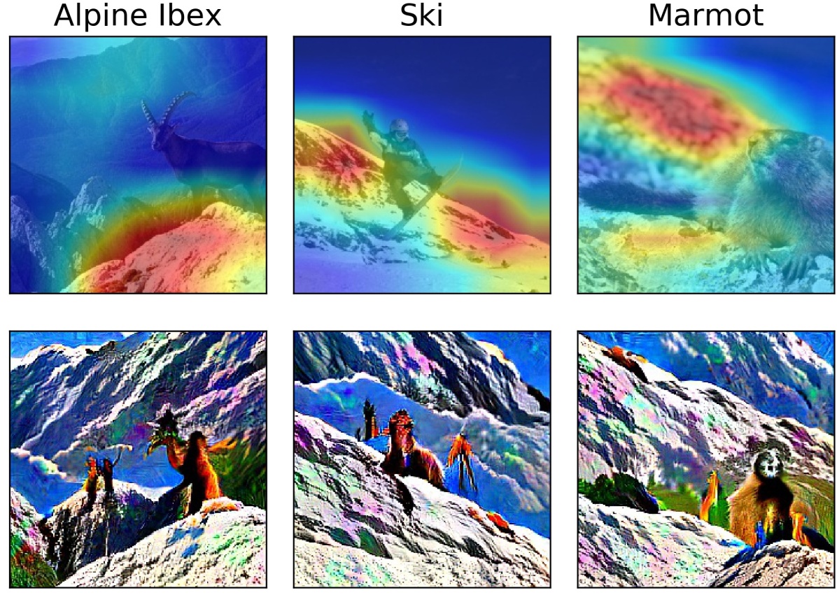
Figure 1: (Top) Regions activating the feature highlighted in red. (Bottom) Images perturbed to visually amplify the feature. The feature (likely mountain) is spurious for $3$ Imagenet classes: Alpine Ibex, Ski, Marmot. Surprisingly, the feature is also core (essential) for $3$ different classes: Mountains, Valley, Volcano.

1 Introduction

Decision making in high-stakes applications such as medicine, finance, autonomous driving, law enforcement and criminal justice is increasingly driven by deep learning models, thereby raising concerns about the trustworthiness and reliability of these systems in the real world. A root cause for the lack of reliability of deep models is their heavy reliance on spurious input features (i.e., features that are not essential to the true label) in their inferences. For example, DeGrave et al. (2021) discovered that a convolutional neural network (CNN) trained to detect COVID-19 from chest radiographs uses spurious text-markers for its predictions. Similarly, Zech et al. (2018) observed that a CNN trained to detect pneumonia from Chest-X rays had unexpectedly learned to identify particular hospital systems with near-perfect accuracy (e.g. by detecting a hospital-specific metal token on the scan) with poor generalization to novel hospital systems. The list of such examples goes on (Beery et al., 2018; de Haan et al., 2019; Bissoto et al., 2020).

To highlight the complexity of this issue, in Figure 1, we show example of a spurious feature that is common across $3$ classes. Surprisingly, this feature is also core (essential) for $3$ other classes showing that while deep models excel at pattern recognition, they can struggle in discerning which patterns are core for a class, at times incorrectly making use of spurious patterns recognized elsewhere.

The standard Empirical Risk Minimization (ERM) paradigm for training deep neural networks is brittle when the test distribution is different from the training distribution because of spurious features. Recently, Arjovsky et al. (2020) proposed a framework called Invariant Risk Minimization (IRM) to address this problem. IRM and its variants (Krueger et al., 2021; Xie et al., 2020; Mahajan et al., 2021) posit the existence of a feature embedder such that the optimal classifier on top of these features is the same for every environment from which data can be drawn. However, Rosenfeld et al. (2021) show that IRM can fail catastrophically unless the test distribution is sufficiently similar to the training distribution. In such cases, however, IRM would no longer be required; we would expect ERM to perform just as well.

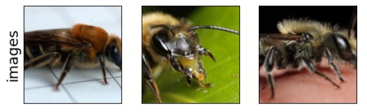
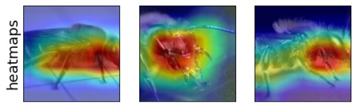
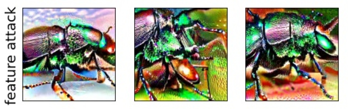
Figure 2: Example of core feature for the class bee.

The above methods use single-label supervision (i.e. an image is labeled only by class index). One can argue that such limited annotations may restrict the model’s ability to learn from meaningful features in its predictions since the model is not given the information regarding which features are essential/core and which ones are redundant/spurious. Much of the prior work on discovering spurious features (Nushi et al., 2018; Zhang et al., 2018; Chung et al., 2019; Xiao et al., 2021) require expensive human-guided labeling of visual attributes, which is not scalable for datasets with a large number of classes and images such as Imagenet. However, Singla & Feizi (2022) recently introduced an approach for discovering spurious features at scale using the neurons of robust models as visual attribute detectors. An application of their approach on a subset of Imagenet (Deng et al., 2009) resulted in a dataset called the Salient Imagenet whose samples, in addition to class labels, are annotated by two sets of masks: core masks that highlight core/essential attributes (with respect to the true class) and spurious masks that highlight attributes co-occurring with the object but not a part of it. While valuable for evalation, the size of the Salient ImageNet dataset ($232$ classes, ${\sim}52$k images) limits its utility for training models.

In this work, we significantly expand the size of the Salient Imagenet dataset in two steps (Section 4). First, for each class $i\in\mathcal{Y}-\mathcal{T}$ (the set of remaining $1000-232=768$ classes), we identify the top-$5$ penultimate layer neurons of a robust model highly predictive of $i$. We then conduct a Mechanical Turk (MTurk) study for each of these (class, neuron) pairs to determine whether the neuron is core or spurious for the class, resulting in new annotations for $768\times 5=3840$ pairs, for a total of $5000$ core/spurious annotations ($4370$ core and $630$ spurious), when combined with those of Singla & Feizi (2022). Second, for each (class=$i$, feature=$j$) pair, we conduct another MTurk study to validate that the neural activation maps (NAMs) for these neurons highlight the same visual attribute for a large number of images. For images with label $i$, we select the subset with the top-$260$ values of feature $j$. Next, we ask workers to validate whether the NAMs of $15$ images (randomly selected from $260$) focus on the same visual attribute. We validate that for $95.26\%$ of pairs, NAMs indeed focus on the same visual attribute. The resulting dataset, called Salient Imagenet-1M, contains more than $1$ million core/spurious mask annotations.

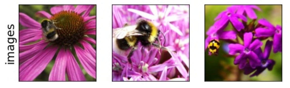
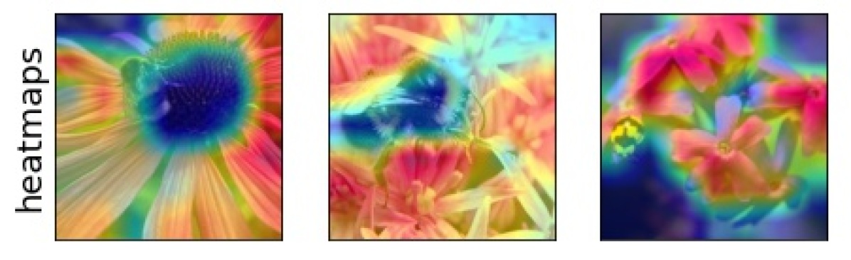
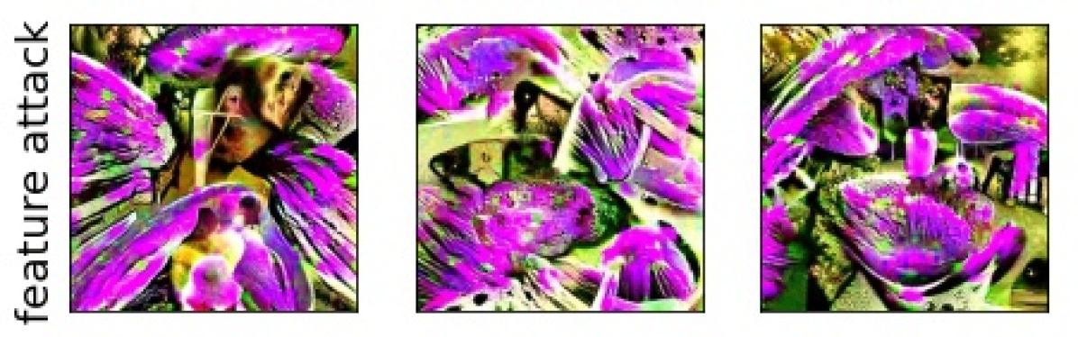
Figure 3: Example of spurious feature for the class bee.

Using our test set, we study a diverse set of pretrained Imagenet models and training paradigms ($42$ models total) in Section 6. We find that: (i) transformers are more sensitive to spurious features compared to Convnets, (ii) adversarial training makes Resnets more sensitive to spurious features, (iii) zero-shot CLIP transformers are highly susceptible to spurious features, (iv) models with the same clean accuracy can have vastly different core accuracy (i.e., accuracy when the non-core regions are corrupted using noise).

We next aim to train models that mainly use core features in their predictions. To this end, we propose a training paradigm called Core Risk Minimization (CoRM) in Section 7. We note that in some cases, spurious features can be useful. Consider the class “matchstick”: the brightness of a flame (spurious) may obscure core features beyond recognition, but the flame itself provides evidence for the presence of a matchstick (see Appendix B). Thus, when core features are absent or not known to be in the image, we want our objective to reduce to standard ERM. Based on this desideratum, we formulate our CoRM objective as follows:

$$\min_{\theta}\ \mathbb{E}_{(\mathbf{x},\mathbf{c},y)}\ \left[\mathbb{E}_{\mathbf{z}\sim\mathbb{N}(\boldsymbol{0},\sigma^{2}\mathbf{I})}\ \ \ell(f_{\theta}(\mathbf{x}^{*}),y)\right]$$ (1)

$$\text{where }\mathbf{x}^{*}=\mathbf{x}+\mathbf{z}\odot(\boldsymbol{1}-\mathbf{c})$$

Here, $\mathbf{c}$ denotes the core mask (i.e., $\mathbf{c}_{i,j}=1$ iff $\mathbf{x}_{i,j}$ is a core pixel), $y$ is the ground truth label for $\mathbf{x}$, $f_{\theta}(\mathbf{x}^{*})$ denotes the logits, $\ell$ is the cross entropy loss and $\theta$ is the model parameters. Note that $\mathbf{x}^{*}_{i,j}=\mathbf{x}_{i,j}\ \ \forall\ i,j:\mathbf{c}_{i,j}=1$ which ensures that $\mathbf{x}^{*}$ will have the same core features as $\mathbf{x}$. However, the non-core regions are corrupted using Gaussian noise with variance $\sigma^{2}$. Note that one can easily modify our CoRM formulation to have corruptions using other noise distributions or even adversarial corruptions on non-core regions. We use Gaussian noise because of its simplicity and because it easily allows us to control the degree of contextual information from non-core regions in the image using the parameter $\sigma$. When the core masks are unknown, we can set $\mathbf{c}_{i,j}=1\ \ (\forall\ i,j)$ so that $\mathbf{x}^{*}=\mathbf{x}$. This allows us to recover the standard ERM objective. Finally, note that our CoRM objective can also be used to train models when the core masks $\mathbf{c}$ are soft (e.g., $0\leq\mathbf{c}_{i,j}\leq 1$ not $\in\{0,1\})$.

In our CoRM objective (1), we need to compute the inner expectation over the Gaussian distribution in a high dimensional space which can be difficult. Thus, to train models using the Salient Imagenet-1M dataset, we evaluate different variations for training using CoRM: (i) randomly adding Gaussian noise to the non-core regions during training, (ii) saliency regularization that penalizes the gradient norm in the non-core (i.e., $\boldsymbol{1}-\mathbf{c}$) regions. We show that by combining these two techniques, we achieve significantly higher $(+12\%)$ core accuracy, while improving the clean accuracy compared to ERM trained models.

In summary, we make the following contributions:

• We introduce the Salient Imagenet-1M dataset with core and spurious masks for more than a million images in all Imagenet classes.

• We comprehensively study the reliance on spurious features for 42 pretrained Imagenet models and training procedures, discovering interesting trends.

• We introduce Core Risk Minimization (CoRM), a new learning paradigm to train models that mainly rely on core features in their predictions, leading to strong empirical results ($+12\%$ core, $+0.58\%$ clean accuracy in Table 1).

2 Related work

Interpretability: Most of the existing works on post-hoc interpretability techniques focus on inspecting the decisions for a single image (Zeiler & Fergus, 2014; Mahendran & Vedaldi, 2016; Dosovitskiy & Brox, 2016; Yosinski et al., 2016; Nguyen et al., 2016; Adebayo et al., 2018; Zhou et al., 2018; Chang et al., 2019; Olah et al., 2018; Yeh et al., 2019; Carter et al., 2019; O’Shaughnessy et al., 2019; Sturmfels et al., 2020; Verma et al., 2020). These include saliency maps (Simonyan et al., 2014; Sundararajan et al., 2017; Smilkov et al., 2017; Singla et al., 2019), class activation maps (Zhou et al., 2016; Selvaraju et al., 2019; Bau et al., 2020; Ismail et al., 2019, 2020), surrogate models to interpret local decision boundaries such as LIME (Ribeiro et al., 2016), methods to maximize neural activation values by optimizing input images (Nguyen et al., 2015; Mahendran & Vedaldi, 2015) and finding influential (Koh & Liang, 2017) or counterfactual inputs (Goyal et al., 2019).

Failure explanation: Recent works (Tsipras et al., 2018; Engstrom et al., 2019) provide evidence that robust models (Madry et al., 2018) are more interpretable than standard models. Thus, some recent works use the penultimate layer neurons of robust models as visual attribute detectors for discovering failure modes. Among these, Wong et al. (2021) can only analyze the failures of robust models which achieve lower accuracy than standard (non-robust) models. Barlow (Singla et al., 2021) can analyze the failures of any model (standard/robust) but is not useful for highly accurate models. The framework of Singla & Feizi (2022) addresses these limitations and is discussed in Section 4.1.

Domain generalization: In this setting, we aim to learn predictors which generalize to test distributions different from training data. The frameworks studied either make assumptions about covariate/label shifts (Widmer & Kubát, 2004; Bickel et al., 2009; Lipton et al., 2018), or that test distribution is in some set around training data (Bagnell, 2005; Rahimian & Mehrotra, 2019), or that training data is sampled from distinct distributions (Blanchard et al., 2011; Muandet et al., 2013; Sagawa* et al., 2020). Many works provide formal guarantees by assuming invariance in the causal structure of the data (Tian & Pearl, 2001; Didelez et al., 2006; Peters et al., 2016; Heinze-Deml et al., 2018; Heinze-Deml & Meinshausen, 2021; Christiansen et al., 2021). IRM (Arjovsky et al., 2020) was also designed for this setting but lacked strong theoretical guarantees. Since then, there have been many works on improving the IRM objective (Xie et al., 2020; Chang et al., 2020; Ahuja et al., 2020; Krueger et al., 2021; Mahajan et al., 2021) and comparing ERM and IRM from theoretical (Ahuja et al., 2021; Rosenfeld et al., 2021, 2022) and empirical perspectives (Gulrajani & Lopez-Paz, 2021).

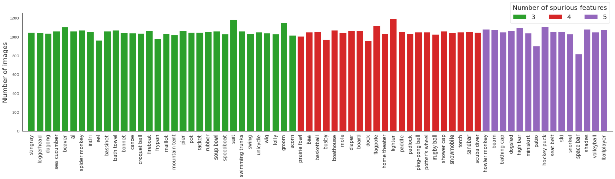
Figure 4: Number of images for classes with at least $3$ spurious features in the Salient Imagenet-1M training set.

3 Notation and Definitions

The activation vector in the penultimate layer (after global average pooling) of a trained neural network is called the neural feature vector. Each element of this vector is called a neural feature. For an image $\mathbf{x}$ and neural feature $j$, we can obtain the Neural Activation Map or NAM (similar to CAM by Zhou et al. (2016)) that provides a soft mask for the highly activating pixels in $\mathbf{x}$ for the feature $j$. The corresponding heatmap can be obtained by overlaying the NAM on top of $\mathbf{x}$ so that the red region highlights the highly activating pixels. The feature attack (Engstrom et al., 2019) is generated by optimizing the image $\mathbf{x}$ to increase the value of feature $j$. These methods are discussed in more detail in Appendix D. For each class $i\in\mathcal{Y}$, we define core features $(\text{denoted by }\mathcal{C}(i))$ as the set of features that are always a part of the object $i$, spurious features $(\text{denoted by }\mathcal{S}(i))$ are the ones that are likely to co-occur with $i$, but not a part of it. Example visualizations for core and spurious features (using heatmaps, feature attack) are in Figures 2 and 3 respectively.

4 Expanding the Salient Imagenet dataset

The original Salient Imagenet dataset introduced by Singla & Feizi (2022) is limited to $232$ classes (denoted by $\mathcal{T}$) with a total size of $52,521$ images ($\approx 226$ images per class). Each instance in the dataset is of the form $(\mathbf{x},y,\mathcal{M}^{c},\mathcal{M}^{s})$ where $y$ is the ground truth label and $\mathcal{M}^{c}/\mathcal{M}^{s}$ denote the set of core/spurious masks for the image $\mathbf{x}$ respectively. By adding noise to the core/spurious regions using these masks and observing the drop in the accuracy, this dataset can be used to test the sensitivity of any pretrained model to different visual features. While useful for evaluating models, the relatively small size of this dataset limits its usefulness for training large models. Thus, our first goal is to significantly expand the size of the Salient Imagenet dataset so that we can use it for training deep models that mainly rely on core features for their inferences.

4.1 Review of the Salient Imagenet Framework

For each class $i\in\mathcal{T}$, using an adversarially trained (robust) model, Singla & Feizi (2022) first identified the $5$ neural features that are most predictive of $i$ using the Neural Feature Importance scores (details in Appendix C) resulting in $232\times 5=1160$ (class, feature) pairs. Next for each class $i\in\mathcal{T}$, they annotated each of these $5$ features as core or spurious using a Mechanical Turk (MTurk) study.

To obtain the core/spurious annotation for each (class=$i$, feature=$j$) pair, they showed the MTurk workers two panels: one describes the class $i$ while the other visualizes the feature $j$. To describe the class $i$, they showed the object names (Miller, 1995), object supercategory (Tsipras et al., 2020), object definition, wikipedia links and $3$ images with label $i$ from the Imagenet validation set. The feature $j$ is visualized using $5$ images with predicted class $i$ that maximally activate the feature $j$, their heatmaps and feature attack visualizations (Examples in Figures 2 and 3).

Next, they asked the workers to determine whether the visual attribute (inferred by visualizing $j$) is a part of the main object (i.e. class $i$), some separate objects, or the background. They also required the workers to provide reasons for their answers and rate their confidence on a likert scale from $1$ to $5$. The design for this study is shown in Appendix Figure 11. Each of these Human Intelligence Tasks (or HITs) were evaluated by $5$ workers. The HITs for which majority of the workers (i.e. $\geq 3$) voted for either separate object or background were deemed to be spurious and the ones with main object as the majority vote were deemed to be core.

4.2 Mechanical Turk studies for Salient Imagenet-1M

Discovering core/spurious features for 768 classes: We used the same procedure discussed in Section 4.1 to obtain core/spurious annotations for the remaining $768$ classes (denoted by $\mathcal{Y}-\mathcal{T}$). Out of the total $768\times 5=3840$ (class, feature) pairs that we evaluated, $3,372$ are deemed to be core and $468$ to be spurious by the workers. On merging the annotations from Singla & Feizi (2022), we obtain such annotations for all $1,000$ classes of Imagenet. In total, we obtain $4,370$ core and $630$ spurious class, feature pairs. For $357$ classes, we discover at least $1$ spurious feature. For $15$ classes, all $5$ features were found to be spurious (shown in Figure 4). We visualize several spurious features in Appendix K.1 (background) and K.2 (foreground).

Discovering large sets of images containing core/spurious features: To further expand the Salient Imagenet dataset, we validate that for the (class=$i$, feature=$j$) pair, the visual attribute inferred by visualizing the feature $j$ (using top-$5$ images with prediction $i$) is also highlighted by the NAMs for the images with ground truth label $i$ and top-$k$ ($k\gg 5$) values of feature $j$. This is expected because in the standard ERM paradigm for training deep models, a model will learn to associate a visual attribute with the class $i$ only if the dataset contains a sufficiently large number of images with ground truth label $i$ containing the same attribute.

To validate that NAMs indeed focus on the desired attributes, we conducted another MTurk study. For the (class=$i$, feature=$j$) pair, we first obtain the training images with label $i$ ($\approx 1300$ images/label in Imagenet) and top-$260$ activations ($20\%$ of $1300$) of the feature $j$. From this set of $260$ images, we selected $5$ images with the lowest activations of feature $j$ and randomly selected $10$ images from the remaining set (excluding the already selected images). We show the workers three panels. The first panel shows images and heatmaps with the highest $5$ activations, the second with next $5$ highest activations and the third with lowest $5$ activations. For each heatmap, workers were asked to determine if the highlighted attribute looked different from at least $3$ other heatmaps in the same panel. Next, they were asked to determine if the heatmaps in the $3$ different panels focused on the same visual attribute, different attributes or if the visualization in any of the panels was unclear. The design of the study is shown in Appendix Figure 12. For all (class, feature) pairs ($1000\times 5=5000$ total), we obtained answers from $5$ workers each. For $4763$ pairs (i.e. $95.26\%$), majority of workers selected same as the answer to both questions. For core features, we observe significantly higher validation rate of $96.48\%\ (4216/4370)$ than for spurious features $86.83\%\ (547/630)$. These results indicate the quality of our annotated masks (specially the core ones) is high.

5 The Salient Imagenet-1M dataset

In Section 4.2, for each class $i\in\mathcal{Y}$, we obtain a set of core and spurious features denoted by $\mathcal{C}(i)$ and $\mathcal{S}(i)$, respectively. We also validated that the NAMs highlight the same visual attribute for a large number of images in $95.26\%$ of all (class=$i$, feature=$j$) pairs. These results enable us to significantly expand the size of the Salient Imagenet dataset and use it for training reliable deep models.

5.1 Train and Test sets of Salient Imagenet-1M

For the Imagenet dataset, the test set was constructed by selecting $50$ images per class resulting in the test set of $50\times 1000=50,000$ images. However, such a test set may not be adequate for testing the sensitivity of a trained model to spurious features because for each class $i\in\mathcal{Y}$, we want our test set to include: (i) a large number of images per spurious feature that the class $i$ is vulnerable to, and (ii) masks for core/spurious regions in these images so that by adding noise to these regions, we can test the sensitivity of the model to these features for making its predictions.

Test set. To construct the test set, for each $i\in\mathcal{Y},j\in\mathcal{C}(i)\cup\mathcal{S}(i)$, we first define $\mathcal{D}(i,j)$ as the set of images with label $i$ and top-$65$ activations of $j$, and their NAMs. The NAMs for these images act as the soft masks that highlight the visual attribute encoded in $j$. If $j\in\mathcal{C}(i)$, these are called core masks and if $j\in\mathcal{S}(i)$ then spurious masks. By taking the union of these sets, i.e., $\cup_{j\in\mathcal{C}(i)\cup\mathcal{S}(i)}\mathcal{D}(i,j)$, we obtain the desired test set for class $i$. In total, the test set contains $226,946$ images across all $1,000$ classes.

Training set. To construct the training set for class $i\in\mathcal{Y}$, we follow the same procedure as above. However, to keep the training and test sets disjoint, we only select images with label $i$ that have not already been included in the test set for class $i$. This results in $1,054,221$ training images for $1000$ classes. We plot the number of images in the training set for classes with at least $3$ spurious features in Figure 4. We note that the NAM validation procedure discussed in Section 4.2 has been performed for top-$260$ images per (class,feature) pair and remaining masks in the training set may not have the same level of quality. However, one can easily specify a constant $k$ to select masks for each (class=$i$, feature=$j$) pair, only for the images with label $i$ and top-$k$ values of $j$.

The union of training and test sets is the Salient Imagenet-1M dataset. We use 1M because the validated dataset contains more than $1$M mask annotations (see Appendix G).

6 Benchmarking pretrained models

In this section, we use Salient Imagenet-1M’s test set to measure the sensitivity of several pretrained models to core/spurious features by computing the degradation in model performance due to Gaussian noise in core/spurious image regions. The premise here is that if a model does not use the content of a region, then adding noise to the region should have no effect. Contrapositively, if adding noise to a region degrades performance, then the model does make use of the region. Singla & Feizi (2022) conducted a similar analysis, introducing the concepts of core accuracy and spurious accuracy, where core/spurious accuracy is (informally) defined to be the model accuracy on images with added noise in the spurious/core regions, respectively. However, their core and spurious accuracy are evaluated only on images that contain the required mask (i.e. only images with spurious masks were included for measuring the core accuracy). In their dataset (as well as our test set), a sample $\mathbf{x}$ contains a mask for feature $j$ only if its activation of $j$ is among the top-$65$ for images from its class, resulting in significantly different data over which core and spurious accuracy were computed.

This results in the following problems: (i) unequal datasets where core/spurious accuracies are computed ($357$ classes have at least $1$ spurious feature while $985$ have at least $1$ core feature), resulting in incomparable numbers, (ii) spurious masks tend to generalize worse than core masks (Section 4.2), thus the computed core accuracy may not be reliable (iii) core and spurious masks can overlap since they are computed using NAM as the soft segmentation masks. To address these limitations, we evaluate each metric only on images with at least $1$ core mask, and compute the spurious mask as the complement of (i.e. $\boldsymbol{1}-$) the mask used for core regions. Furthermore, we employ a new metric, the Relative Core Sensitivity, that combines core and spurious accuracy to quantify model reliance on core features, while controlling for general noise robustness. Lastly, our analysis is significantly larger than that of Singla & Feizi (2022), both in the number of classes and models considered.

6.1 Revised Core and Spurious Accuracy

Each image in the Salient Imagenet-1M test set may have up to five NAMs for core features. Similar to Singla & Feizi (2022), for each image, we take the elementwise maximum of the NAMs for its core features to come up with a single consolidated core mask per image (referred to as $\mathbf{c}$). We also observe that in practice, the core masks often do not cover the entirety of the core region (Figure 5 top left). To ameliorate this, we apply a dilation transform that iteratively replaces each pixel value with the maximum pixel value within a small square kernel (Figure 5, second column).

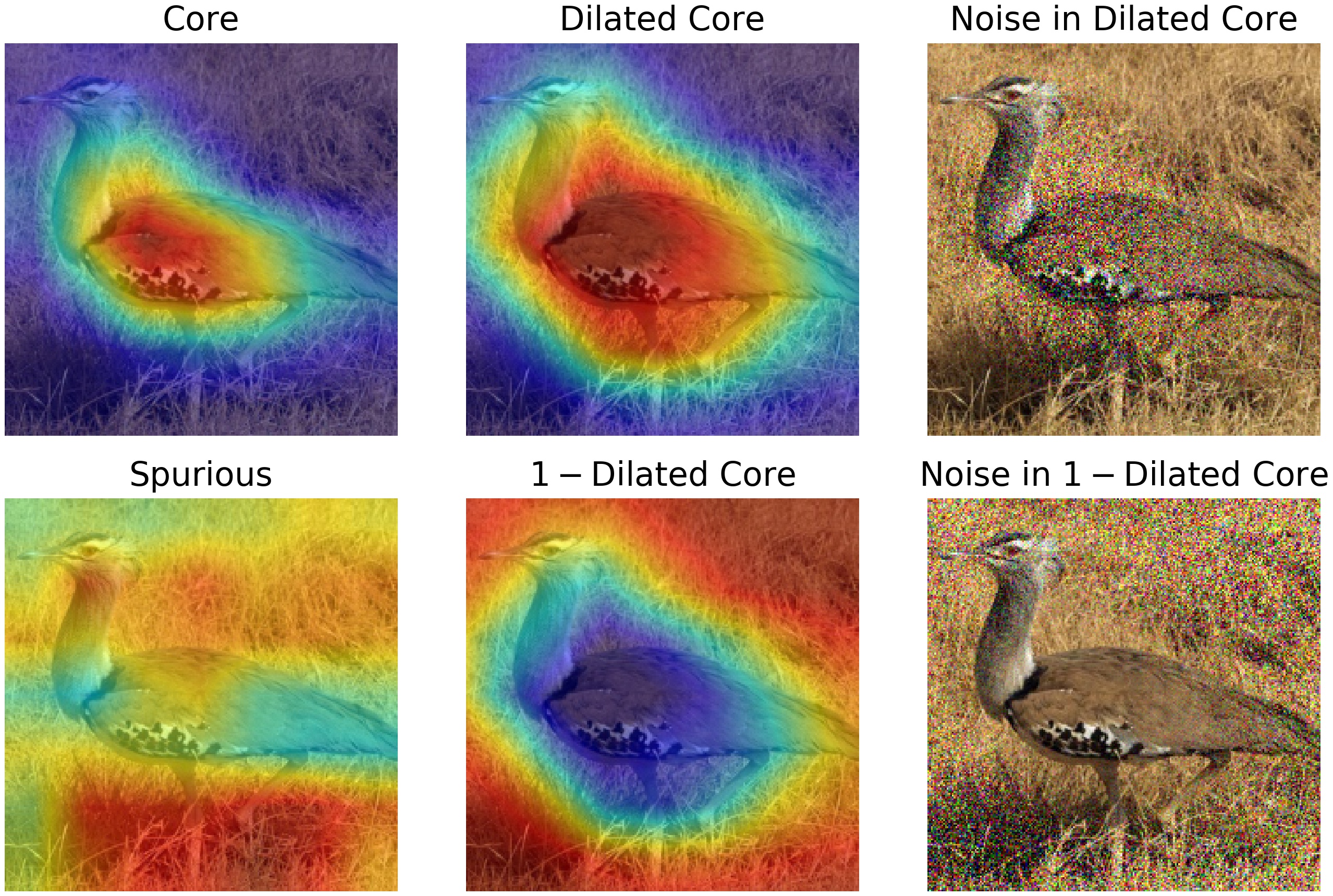
Figure 5: Raw and dilated core masks. First column corresponds to masks used by Singla & Feizi (2022) to compute spurious and core accuracies, while second column corresponds to masks used in this work. Third column shows noise $(\sigma=0.25)$ applied.

Definition 6.1.

(Dilated Core Mask) For mask $\mathbf{m}$, $1$ iteration of dilation with square kernel of side $2k+1$ is defined:

$$[\text{dil}(\mathbf{m})]_{p,q}=\max_{u,v\ \in\ [-k,k]}\mathbf{m}_{p+u,q+v}$$

The dilated core mask, denoted as $\tilde{\mathbf{c}}$, is obtained by applying 15 iterations of dilation using $k=2$ on the core mask $\mathbf{c}$.

In Figure 5, we visualize the difference in core/spurious mask computation procedures between our work and Singla & Feizi (2022). In the left column, we see that using spurious masks obtained in the same manner as core masks (i.e. by taking the max over NAMs of spurious features) may introduce an incongruity in what is considered core and spurious. Specifically, while the spurious mask in the bottom left focuses on the background, it also covers much of the core region. However, the $\boldsymbol{1}-\tilde{\mathbf{c}}$ mask (middle column) by design has low overlap with the dilated core mask $(\tilde{\mathbf{c}})$.

Using these dilated core masks for each sample in the Salient Imagenet-1M test set, we can now define our revised versions of core and spurious accuracy as follows:

Definition 6.2.

(Core and Spurious Accuracy) The Core Accuracy, $\mathrm{acc^{(\mathcal{C})}}$ for a model $h$ is defined as follows:

$$\mathrm{acc^{(\mathcal{C})}}\ =\frac{1}{|\mathcal{Y}|}\sum_{i\in\mathcal{Y}}\frac{1}{|\mathcal{D}\mathcal{C}(i)|}\sum_{\mathbf{x}\in\mathcal{D}\mathcal{C}(i)}\mathbbm{1}(h(\mathbf{x}^{*})=i)$$

$$\text{where }\mathbf{x}^{*}=\mathbf{x}+\sigma(\mathbf{z}\odot(\boldsymbol{1}-\tilde{\mathbf{c}})),\quad\mathbf{z}\sim\mathcal{N(\boldsymbol{0},\mathbf{I})}$$

where $\mathcal{D}\mathcal{C}(i)=\cup_{j\in\mathcal{C}(i)}\mathcal{D}(i,j)$. The Spurious Accuracy, $\mathrm{acc^{(\mathcal{S})}}$ is defined similarly using $\mathbf{x}^{*}=\mathbf{x}+\sigma(\mathbf{z}\odot\tilde{\mathbf{c}})$.

We use $\sigma=0.25$ for all experiments (Figure 5 last column).

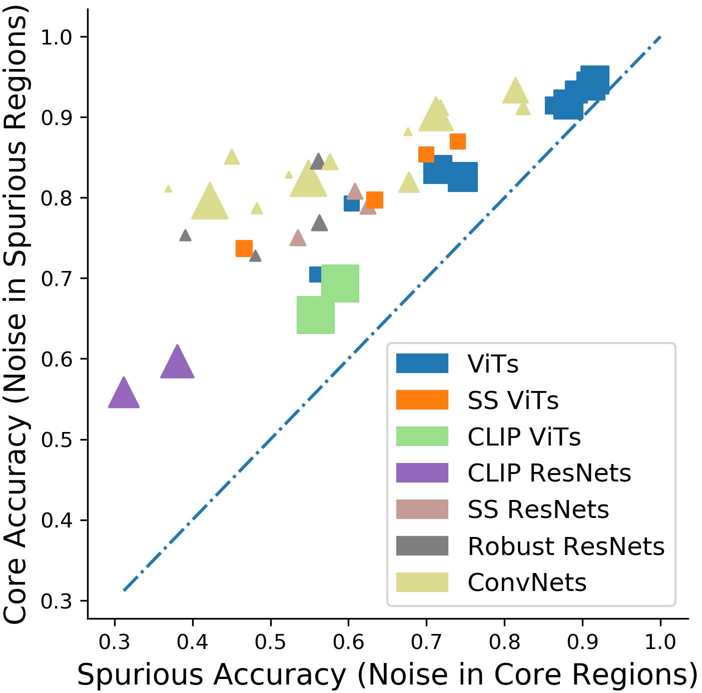
Figure 6: Core/Spurious accuracy evaluated with $\sigma=0.25$. Models with transformer (convolution) architectures have square (triangle) markers. Marker size is proportional to parameter count.

6.2 Relative Core Sensitivity

A limitation of using noise to measure model sensitivity to different image regions is that models extremely robust to noise corruptions will have high core and spurious accuracy and thus less gap between the two (regardless of its use of spurious features). Thus, we introduce a new metric: Relative Core Sensitivity that quantifies the model reliance on core features while controlling for general noise robustness (adapted from a similar metric in Moayeri et al. (2022)):

Definition 6.3.

(Relative Core Sensitivity) We define the Relative Core Sensitivity or $\mathrm{RCS}$ as follows:

$$\mathrm{RCS}:=\frac{\mathrm{acc^{(\mathcal{C})}}-\mathrm{acc^{(\mathcal{S})}}}{2\min(\bar{a},1-\bar{a})},\ \text{where }\bar{a}=\frac{(\mathrm{acc^{(\mathcal{C})}}+\mathrm{acc^{(\mathcal{S})}})}{2}$$

Here, $\bar{a}$ acts as a proxy for the general noise robustness of the model under inspection. We can show that for all models with $\bar{a}$ noise robustness, 2$\min(\bar{a},1-\bar{a})$ is the maximum possible gap between the core/spurious accuracy. Thus, $\mathrm{RCS}$ normalizes the gap in the current model by the total possible gap. In Figure 6, higher $\mathrm{RCS}$ corresponds to lying higher above the diagonal (high core and low spurious accuracy). We derive this metric in more detail in Appendix H.

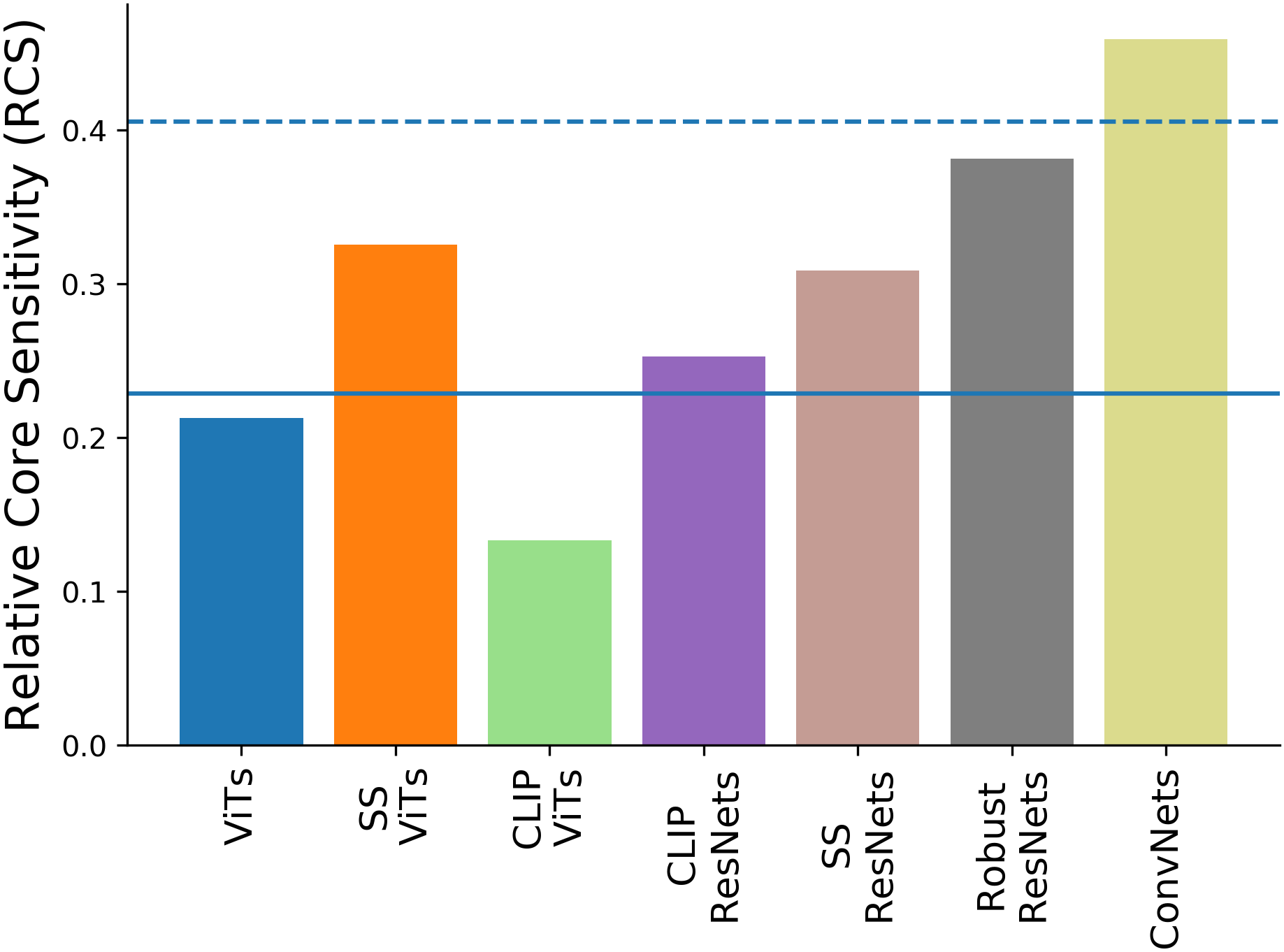
Figure 7: Average $\mathrm{RCS}$ values grouped by model architecture and training procedure. Solid line is average for transformer models ($\mathrm{RCS}=0.23$), dashed for convolutional models ($\mathrm{RCS}=0.41$).

6.3 Findings

We study a large and diverse set of pretrained Imagenet models and training paradigms ($42$ models in total), namely ConvNets (Simonyan & Zisserman, 2014; He et al., 2016; Zagoruyko & Komodakis, 2016; Sandler et al., 2018; Xie et al., 2017; Szegedy et al., 2017; Tan & Le, 2019; Tan et al., 2019), ViTs (Dosovitskiy et al., 2020; Touvron et al., 2021; d’Ascoli et al., 2021; Liu et al., 2021), Robust ResNets (Salman et al., 2020), self-supervised (SS) models on ViT and ResNet arches (Chen* et al., 2021; Caron et al., 2021; Chen et al., 2020), zero-shot models such as CLIP ResNets, CLIP ViTs (Radford et al., 2021). Details in Appendix A.

Figure 6 shows the core and spurious accuracy for all model categories evaluated. We observe that transformer models (squares) lie closer to the diagonal than convolutional models (triangles) suggesting they rely more on spurious features. We hypothesize that the lack of a proper inductive bias in transformers may lead to this phenomenon. We show the average $\mathrm{RCS}$ values in Figure 7 (high $\mathrm{RCS}$ implies high core and low spurious accuracy). We again validate that the transformer models have significantly lower $\mathrm{RCS}$ ($0.23$ compared to $0.41$ for convolutional models). In Appendix Table 2, we observe that zero-shot CLIP ViTs yield the lowest $\mathrm{RCS}$ value. We conjecture that the use of text tokens in zero-shot CLIP models may introduce an additional source of spurious vulnerabilities. We also observe that adversarial training in ResNets decreases $\mathrm{RCS}$ from $0.44$ to $0.38$. A similar result was also observed by Moayeri et al. (2022) in a different setup (details in Appendix I). Moreover, our analysis indicates that the standard accuracy is not sufficient to fully characterize model quality; i.e., different models may have different core accuracy even with the same standard accuracy. For example, EfficientNet-B4 and Inception-V4 (Appendix Table 2) have almost the same clean accuracy ($0.37\%$ gap) but vastly different core accuracy ($9.23\%$ gap).

Training Procedure	Clean Accuracy ($\uparrow$)	Core Accuracy ($\uparrow$)	Spurious Accuracy ($\downarrow$)	$\mathrm{RCS}$ ($\uparrow$)
Baseline (ERM)	74.37% $\pm$ 0.67	52.02% $\pm$ 1.95	12.12% $\pm$ 1.75	0.624 $\pm$ 0.035
Random $\boldsymbol{1}-\mathbf{c}$ Noising	73.74% $\pm$ 0.69	59.23% $\pm$ 6.36	11.49% $\pm$ 5.67	0.692 $\pm$ 0.102
Saliency Regularization	75.06% $\pm$ 0.11	54.37% $\pm$ 1.66	12.37% $\pm$ 2.39	0.633 $\pm$ 0.053
Rand Noising + Sal Reg	74.95% $\pm$ 0.19	63.86% $\pm$ 2.92	8.97% $\pm$ 2.95	0.759 $\pm$ 0.063

Table 1: Model performance using various approaches to CoRM. The final row shows a combination of Random $\boldsymbol{1}-\mathbf{c}$ noising and Saliency regularization results in $11.84\%$ increase in core accuracy and $0.58\%$ increase in clean accuracy. Results averaged over $4$ trials.

7 Core Risk Minimization (CoRM)

ERM yields classifiers that achieve impressive accuracy but it cannot guide models to learn that certain image regions should inform the class label more than others. Models that use spurious features can give a false of sense of performance, as accuracy can drop dramatically in a new domain where correlations between class labels and spurious features are broken. A model that faithfully learns concepts should rely more on core features than on spurious ones.

We formalize this notion in Core Risk Minimization, defined in optimization (1). CoRM seeks to minimize the expected loss over samples with Gaussian noise added in non-core regions. When all image regions are deemed to be core, CoRM reduces to ERM. However, when informative core masks are available, CoRM requires that the optimal classifier remains accurate in spite of corruption in the spurious regions. Cost of data collection previously inhibited the pursuit of CoRM-like learning. Salient Imagenet-1M’s rich core/spurious annotations have the potential to enable training of models that make predictions while avoiding spurious shortcuts. We outline our relaxations to the CoRM objective that lead to significant increases in core accuracy and $\mathrm{RCS}$.

7.1 Relaxing CoRM

First, we approximate the inner expectation of CoRM with a single sample. That is, for each input $(\mathbf{x},\mathbf{c})$ with label $y$, we draw a random noise vector $\mathbf{z}\sim\mathcal{N}(\mathbf{0},\ \sigma^{2}\mathbf{I})$, and use

$$\mathbb{E}_{\mathbf{x}^{*}\sim\mathbb{P}(\mathbf{x},\mathbf{c},\sigma)}[\ell(f_{\theta}(\mathbf{x}^{*}),y)]\approx\ell(f_{\theta}(\mathbf{x}+(\boldsymbol{1}-\mathbf{c})\odot\mathbf{z}),y)$$

Next, to obtain $\mathbf{c}$ for any sample $\mathbf{x}\in i$ in Salient Imagenet, we use the NAMs for all core features $\mathcal{C}(i)$, regardless of the activation of $\mathbf{x}$ on the feature. This differs from the test-set computation of $\mathbf{c}$, and introduces noisier core masks, but facilitates a massive increase in training set size. We note that $\mathbf{c}$ can be dilated (or eroded) to any degree, introducing a hyperparameter allowing the practitioner to choose the amount of surrounding context the model can use without penalty. While $\sigma$ alters the magnitude of corruption, dilation alters the region of corruption, introducing a spatial bias in favor of spurious features that are near the core ones. In our experiments, we train on masks $\mathbf{c}$ with no dilation applied.

7.2 Methods

We explore two efficient approaches to perform CoRM and ultimately reduce the reliance on spurious features: (i) random $\boldsymbol{1}-\mathbf{c}$ noising and (ii) saliency regularization. Following directly from the relaxed formulation of CoRM, $\boldsymbol{1}-\mathbf{c}$ noising minimizes risk on samples augmented with additive Gaussian noise scaled by $\boldsymbol{1}-\mathbf{c}$. In practice, we find that deep networks overfit to noise in the non-core regions, leading to degraded clean accuracy. However, witholding the additive noise for randomly selected batches (e.g., with probability with $p=0.5$) during training leads to a better trade-off between clean and core accuracies.

A second approach utilizes gradient information to perform saliency regularization. Such regularization has been shown to improve generalization (Simpson et al., 2019), robustness to distribution shift in non-core regions (Chang et al., 2021), and model interpretability (Ismail et al., 2021). Formally, for a sample $\mathbf{x}$ with core region $\mathbf{c}$ and label $y$, saliency regularization introduces the following loss term:

$$\mathcal{L}_{sal}=\|(\boldsymbol{1}-\mathbf{c})\odot\nabla_{\mathbf{x}}\ell(f_{\theta}(\mathbf{x}),y)\|^{2}$$

where $\ell$ is the classification loss. We compute the saliency penalty after a full forward and backward pass, as the input gradients are then readily available. Model parameters $\theta$ are then updated to minimize $\mathcal{L}_{sal}$. Notice that because saliency regularization and spurious noising affect opposite ends of the training pipeline (pre-forward pass vs. post-backward pass), they can be combined easily.

7.3 Findings

We train Resnet-50 models on Salient Imagenet-1M, employing the two aforementioned methods and their combinations, as well as a baseline model that uses the standard paradigm, ERM. We seek to demonstrate the feasibility of methods toward achieving CoRM’s objective, not to obtain highest possible accuracies. Thus, we do not perform data augmentation. We provide details about how data augmentation can be used with Salient Imagenet-1M masks in Appendix J. In addition to clean accuracy, we present core and spurious accuracy, as well as $\mathrm{RCS}$, each computed over the test set of Salient Imagenet-1M, following the evaluation protocol of Section 6.

Table 1 summarizes the results. We find that random $\boldsymbol{1}-\mathbf{c}$ noising increases core accuracy by $7.21\%$ relative to baseline. Saliency regularization has a more modest improvement in core accuracy, but improves clean accuracy. Combining the two methods yields a $11.84\%$ increase in core accuracy, while also marginally improving clean accuracy. Moreover, spurious accuracy decreases significantly, causing a large improvement of $0.13$ in $\mathrm{RCS}$. These preliminary results suggest that the goals of achieving high clean accuracy while also maintaining high core accuracy and having a low spurious accuracy can be made feasible through Salient Imagenet-1M. We hope that our introduced dataset and training methods will lead to the development of deep models that mainly rely on core features for their inferences.

Appendix

Appendix A Details on Pretrained Models

Model	Clean Accuracy	Core Accuracy	(Drop)	Spurious Accuracy	(Drop)	RCS
ConViT-T/16	87.23%	84.30 %	(-2.92%)	76.95%	(-10.27%)	18.97
ConViT-S/16	92.85%	91.62 %	(-1.23%)	88.16%	(-4.69%)	17.11
ConViT-B/16	94.83%	93.83 %	(-1.00%)	91.07%	(-3.76%)	18.29
DeiT-T/16	86.81%	83.45 %	(-3.36%)	75.26%	(-11.55%)	19.83
DeiT-S/16	93.06%	91.44 %	(-1.61%)	87.06%	(-5.99%)	20.38
DeiT-B/16	95.76%	94.62 %	(-1.13%)	91.61%	(-4.14%)	21.85
Swin-B/4 Window7	92.93%	91.58 %	(-1.35%)	88.19%	(-4.73%)	16.73
Swin-S/4 Window7	93.58%	93.12 %	(-0.46%)	89.22%	(-4.36%)	22.07
Swin-T/4 Window7	92.19%	91.45 %	(-0.74%)	86.33%	(-5.86%)	23.05
ViT-T/16	61.06%	36.81 %	(-24.25%)	11.73%	(-49.33%)	51.66
ViT-S/16	87.59%	79.24 %	(-8.35%)	60.43%	(-27.16%)	31.18
ViT-S/32	80.65%	70.46 %	(-10.19%)	56.01%	(-24.64%)	19.65
ViT-B/16	88.68%	83.51 %	(-5.17%)	71.45%	(-17.23%)	26.76
ViT-B/32	87.62%	82.55 %	(-5.07%)	74.67%	(-12.95%)	18.42
DINO ViTs8	92.05%	86.94 %	(-5.12%)	74.02%	(-18.04%)	33.09
DINO ViTs16	91.16%	85.33 %	(-5.83%)	69.95%	(-21.21%)	34.39
DINO ResNet50	87.03%	80.81 %	(-6.22%)	60.79%	(-26.24%)	34.28
MoCo-v3 ViT-S/	84.38%	73.67 %	(-10.71%)	46.63%	(-37.75%)	33.93
MoCo-v3 ViT-B/	87.38%	79.73 %	(-7.65%)	63.34%	(-24.03%)	28.78
MoCo-v3 ResNet50	85.37%	78.95 %	(-6.42%)	62.45%	(-22.92%)	28.16
CLIP ViT-B/16	76.62%	69.32 %	(-7.31%)	58.92%	(-17.70%)	14.48
CLIP ViT-B/32	73.08%	65.41 %	(-7.67%)	55.83%	(-17.25%)	12.16
CLIP ResNet50	68.71%	55.85 %	(-12.85%)	31.18%	(-37.52%)	28.34
CLIP ResNet101	70.93%	59.73 %	(-11.20%)	38.00%	(-32.93%)	22.23
EfficientNet B0	89.52%	88.23 %	(-1.29%)	67.60%	(-21.92%)	46.70
EfficientNet B4	87.18%	91.16 %	(3.98%)	82.32%	(-4.85%)	33.31
Inception V4	87.55%	81.93 %	(-5.62%)	67.70%	(-19.85%)	28.25
MnasNet A1	86.28%	82.87 %	(-3.41%)	52.30%	(-33.98%)	47.15
MobileNetv2 100	83.82%	81.15 %	(-2.67%)	36.88%	(-46.94%)	54.02
ResNet18	85.42%	78.69 %	(-6.73%)	48.21%	(-37.21%)	41.69
ResNet34	84.69%	85.12 %	(0.43%)	45.00%	(-39.69%)	57.40
ResNet50	92.22%	84.47 %	(-7.75%)	57.59%	(-34.64%)	46.39
Resnext50 32X4D	88.07%	91.19 %	(3.12%)	71.78%	(-16.28%)	52.41
Robust ResNet18 Eps1	86.44%	75.37 %	(-11.08%)	39.06%	(-47.39%)	42.43
Robust ResNet18 Eps3	80.81%	72.81 %	(-8.00%)	48.04%	(-32.77%)	31.30
Robust ResNet50 Eps1	91.66%	84.56 %	(-7.10%)	56.12%	(-35.53%)	47.93
Robust ResNet50 Eps3	81.98%	76.90 %	(-5.08%)	56.26%	(-25.72%)	30.88
SimCLR ResNet50X1	87.13%	75.06 %	(-12.07%)	53.46%	(-33.66%)	30.21
Vgg19	91.03%	79.66 %	(-11.37%)	42.17%	(-48.85%)	47.95
Vgg19 Bn	90.29%	82.44 %	(-7.85%)	54.83%	(-35.46%)	44.02
Wide ResNet50	93.09%	93.36 %	(0.27%)	81.40%	(-11.68%)	47.36
Wide ResNet101	91.53%	90.45 %	(-1.08%)	71.18%	(-20.35%)	50.21

Table 2: Complete results for evaluation of several pretrained Imagenet models. We present core accuracy, spurious accuracy, and $\mathrm{RCS}$, as described in section 6. All metrics are computed over the test set of Salient-Imagenet-1M.

In Section 6, we present a framework for evaluating the reliance on spurious features of any model pretrained on ImageNet, and present results for a breadth of models. We now share greater detail on the models studied and the the results obtained in Table 2. For consistency, we obtain nearly all pretrained weights from the timm framework (Wightman, 2019), with the exception of self-supervised and CLIP model weights, which were obtained directly from the original sources, and adversarially trained networks, obtained from (Salman et al., 2020).

We study a large set of pretrained ImageNet models ($42$ total), spanning various architectures and training paradigms:

Convolution-based models: ResNets (He et al., 2016), Wide ResNets (Zagoruyko & Komodakis, 2016), ResNext (Xie et al., 2017), Inceptionv2 (Szegedy et al., 2017), VGG (Simonyan & Zisserman, 2014), Efficientnet (Tan & Le, 2019), MNasNet (Tan et al., 2019), and MobileNetv2 (Sandler et al., 2018). We refer to this group as ConvNets.

Vision Transformer-based models: ViT (Dosovitskiy et al., 2020), DeiT (Touvron et al., 2021), ConViT (d’Ascoli et al., 2021), and Swin Transformers (Liu et al., 2021). We refer to this group as ViTs.

Robust ResNets: Adversarially trained Resnets with $\ell_{2}$ projected gradient descent (Salman et al., 2020). We refer to this group as Robust ResNets.

Self-supervised models: MoCo-v3 (Chen* et al., 2021), DINO (Caron et al., 2021), and SimCLR (Chen et al., 2020), on both transformer and ResNet backbones, yielding the groups SS ViTs and SS ResNets. SS Models are evaluated with a linear layer trained atop fixed features with full supervision (as is standard practice).

CLIP models: Zero-shot classification models based on CLIP (Radford et al., 2021), again both transformers and ResNets. We follow the zero-shot evaluation procedure of comparing the dot product of an image encoding to the average encoded vector of eight template text captions per class.

A.1 Additional Observations

Model size has small and inconsistent effects on $\mathrm{RCS}$, which allows for comparing averages across categories with varying model sizes. The primary trend of transformers having lower $\mathrm{RCS}$ than ConvNets is validated in the smaller cohort of CLIP models, where the average $\mathrm{RCS}$ decreases from $0.25$ for CLIP ResNets to $0.13$ for CLIP ViTs. However, for self-supervised models MoCo-v3 and DINO, transformers and ResNets yield similar sensitivities. Interestingly, for ResNet backbones, self-supervised training decreases $\mathrm{RCS}$ (-$0.15$), while the reverse is true for transformers ($+0.10$).

Surprisingly, we observe that adversarial training in ResNets decreases $\mathrm{RCS}$ from $0.44$ to $0.38$, despite their objective of making models more reliable through increasing adversarial robustness. Further, the attack budget $\epsilon$ used during training, with higher attack budget leading to more robustness, validates our observed trend, as the gap in $\mathrm{RCS}$ between Robust Resnets and Resnets is larger for robust models with $\epsilon=3$ than for those with $\epsilon=1$.

Lastly, we find that increasing patch size in some ViTs leads to large drops in $\mathrm{RCS}$. Specifically, changing patchsize from 16 to 32 reduces $\mathrm{RCS}$ from $0.14$ to $0.12$ for CLIP ViTs, and from $0.29$ to $0.19$ for (Dosovitskiy et al., 2020)’s original ViT.

A.2 Conjectures

We stress that detailed experiments are necessary to rigorously make further claims regarding our observations. However, we are intrigued by the low $\mathrm{RCS}$ in transformers. Further, the conflicting effect of self-supervision across architectures suggests there may be more factors at play. Vision transformers are emerging rapidly, and most transformer-based models (including DeiT, ConViT, and Swin) follow the training procedure of Touvron et al. (2021), where data-efficiency was achieved via heavy augmentation. Augmentation is also used in self-supervised learning, to create multiple views of the same image. Seeing as many modern augmentations potentially corrupt core regions, we ponder if the increased gain in test accuracy may come at the cost of raising sensitivity to spurious regions. Further experimentation in this direction may be of interest.

Appendix B Role of Spurious Features in Robust Resnet-50 Predictions

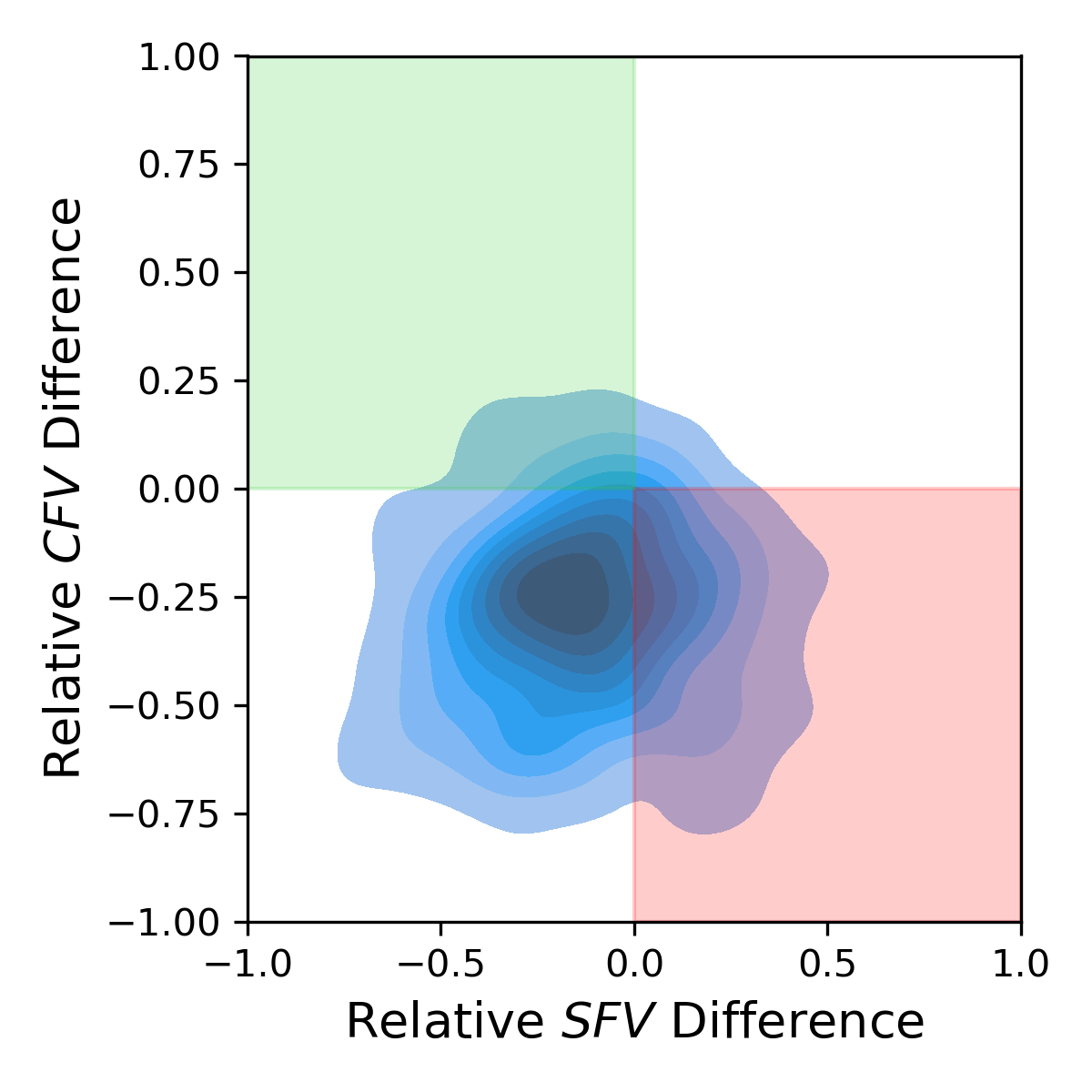
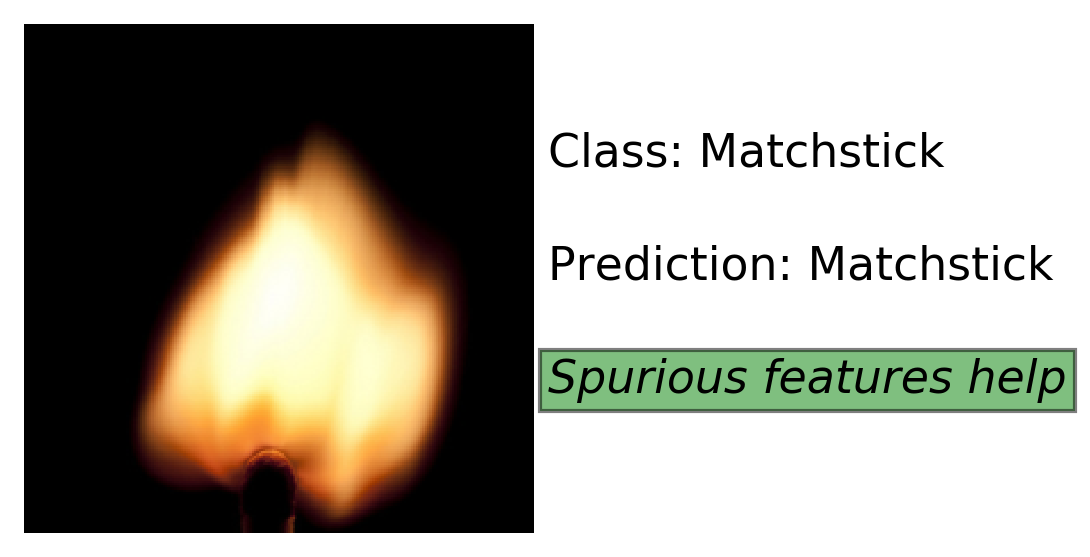
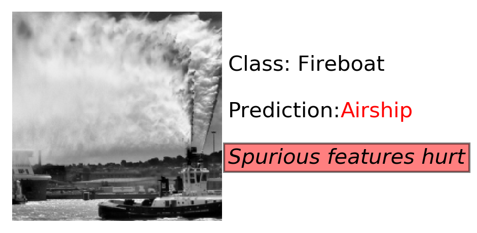
Figure 8: Spurious correlations help and hurt classifiers. (Left) Distribution per class of the relative difference in average core and spurious feature values between misclassified (MC) and correctly classified (CC) samples to the class. (Right) Examples of classes where spurious features help correct classification (top) and where they lead to misclassification (bottom, original class: fireboat).

In this section, we motivate the study of spurious correlations through an error analysis. Importantly, this analysis makes no use of additive noise to gauge sensitivity, offering a distinct and complementary perspective to our other findings. Specifically, we use the annotations of neural nodes in the Robust Resnet-50 used to generate NAMs, directly inspecting feature activations. We first outline the intuition and key takeaways, before delving into detailed discussion of methods and results.

B.1 The Matchstick Example: Spurious features can help or hurt, depending on class

In Figure 8, we display two samples where the spurious feature value of the predicted class is much higher, but core feature values are significantly lower, when compared to the average for correctly classified images of the class. Thus, the prediction is made due to the activations of the class’ spurious features. For the matchstick, recognizing the spurious feature of the flame compensated for the fact that most of the matchstick lies outside of the image region, leading to a correct classification. However, the fireboat is misclassified as an airship, due to the spurious feature of what seems like a cloudy sky.

The analysis of this section inspects core and spurious feature values for correct and incorrect classifications on a classwise basis. We find that spurious features hurt (i.e. activate higher for misclassified samples, even when core features correctly activate lower) much more often than they help (i.e. activate higher for true instances of the class, even when core features incorrectly activate lower). Specifically, for classes where the difference in spurious and core feature values between misclasssified and correctly classified samples have opposite sign ($101$ classes), the spurious features hurt $85\%$ of the time.

This offers quantitative evidence to how spurious features lead to misclassification in a model trained with single-label supervision. However, we also demonstrate the how the role of spurious correlations varies, even from class to class. In summary, spurious features can be harmful, but true understanding of their roles requires careful analysis. We hope Salient Imagenet-1M opens the door to inquiries of this kind.

B.2 Methodology for Error Analysis

For an image $\mathbf{x}$ from class $i$ with core features $\mathcal{C}(i)$ and spuriuos features $\mathcal{S}(i)$, denote the representation vector (i.e. activations of neurons in penultimate layer of Robust Resnet-50) for $\mathbf{x}$ as $\mathbf{r}(\mathbf{x})$. For a set $\mathcal{X}$, we measure the average activation of core features as follows:

Definition B.1.

(Core Feature Value) We define core feature value over a set of inputs $\mathcal{X}$, for both a class-feature pair $(i,j)$ and a single class $i$ (denoted $\mathrm{CFV}_{i,j}$ and $\mathrm{CFV}_{i}$ respectively) as follows:

$$\mathrm{CFV}_{i}(\mathcal{X}):=\frac{1}{|\mathcal{C}(i)|}\sum_{j\in\mathcal{C}(i)}\mathrm{CFV}_{i,j}(\mathcal{X}),\text{ with }\mathrm{CFV}_{i,j}(\mathcal{X}):=\frac{1}{|\mathcal{X}|}\sum_{\mathbf{x}\in\mathcal{X}}\mathbf{r}_{j}(\mathbf{x})$$

We can analogously define spurious feature value for a class $i$ and set $\mathcal{X}$ by replacing $\mathcal{C}(i)$ with $\mathcal{S}(i)$ in B.1.

We now define groups $\mathcal{CC}_{i},\mathcal{MC}_{i}$, corresponding to correctly and incorrectly classified samples to class $i$ (i.e. by prediction). That is, with $h$ denoting the Robust Resnet-50,

$$\mathcal{CC}_{i}=\{\mathbf{x}\in i|h(\mathbf{x})=i\},\mathcal{MC}_{i}=\{\mathbf{x}\not\in i|h(\mathbf{x})=i\}$$

Using the above notation, we obtain the metrics presented in the figure 8. Specifically, Relative $\mathrm{CFV}$ Difference refers to:

Definition B.2.

(Relative $\mathrm{CFV}$ Difference)

$$\text{Relative }\mathrm{CFV}\text{ Difference}(i)=\frac{\mathrm{CFV}_{i}(\mathcal{MC}_{i})-\mathrm{CFV}_{i}(\mathcal{CC}_{i})}{\max(\mathrm{CFV}_{i}(\mathcal{MC}_{i}),\mathrm{CFV}_{i}(\mathcal{CC}_{i}))}$$

This metric lies between $-1$ and $1$. When the relative $\mathrm{CFV}$ difference of a class $i$ is positive, that entails that misclassified samples activate the core features for the class more than correctly classified samples. Relative $\mathrm{SFV}$ Difference is defined analogously by replacing $\mathrm{CFV}$ with $\mathrm{SFV}$.

For classes with at least one spurious and one core feature (324 total), we evaluate relative $\mathrm{CFV}$ difference and relative $\mathrm{SFV}$ difference, using images in the test set of Salient Imagenet-1M (though the analysis does not require core and spurious masks). We display the kernel destiny estimate of the distribution of (relative $\mathrm{SFV}$ difference, relative $\mathrm{CFV}$ difference) pairs in figure 8.

B.3 Findings

For $84$ classes, relative $\mathrm{SFV}$ difference is positive while the relative $\mathrm{CFV}$ difference is negative (red quandrant). This suggests that the incorrect prediction of misclassified samples is due to high activation of spurious features, and not core features. Conversely, for $17$ classes, the reverse is true (green quadrant in fig. 8), suggesting that core features erroneously activate higher for misclassifications. However, the spurious feature activations are higher for instances of the class, correcting the mistakes of the core features. Thus, spurious features can both help and hurt classifiers, and their role varies significantly based on class. We highlight this result, as it reflects the complicated nature of spurious features, and their roles in deep models. We believe the complete removal of spurious features may have unintended consequences, and suggest careful analysis, with respect to class, when addressing spurious features.

Appendix C Selecting the neural features highly predictive of the class

The neural feature vector (i.e the vector of penultimate layer neurons) can have a large size ($2048$ for the Robust Resnet-50 used in this work and the prior work of Singla & Feizi (2022)) and visualizing all of these features for a particular class (say class $i$) to determine whether they are core or spurious for $i$ can be difficult. Thus, we select a small subset of these features that are highly predictive of class $i$ and annotate them as core or spurious for $i$ using the same method as used in the prior work of Singla & Feizi (2022).

We first select a subset of images (from the training set) on which the robust model predicts the class $i$. We compute the mean of neural feature vectors across all images in this subset denoted by $\overline{\mathbf{r}}(i)$. From the weight matrix $\mathbf{w}$ of the last linear layer of the robust model, we extract the $i^{th}$ row $\mathbf{w}_{i,:}$ that maps the neural feature vector to the logit for the class $i$. Next, we compute the hadamard product $\overline{\mathbf{r}}(i)\odot\mathbf{w}_{i,:}$. Intuitively, the $j^{th}$ element of this vector $(\overline{\mathbf{r}}(i)\odot\mathbf{w}_{i,:})_{j}$ captures the mean contribution of neural feature $j$ for predicting the class $i$. This procedure leads to the following definition:

Definition C.1.

The Neural Feature Importance of feature $j$ for class $i$ is defined as: $\mathrm{IV}_{i,j}=\left(\overline{\mathbf{r}}(i)\odot\mathbf{w}_{i,:}\right)_{j}$. For class $i$, the neural feature with $k^{th}$ highest $IV$ is said to have the feature rank $k$.

We then select the neural features with the highest-$5$ importance values (defined above) per class.

Appendix D Visualizing the neural features of a robust model

D.1 Heatmap

Heatmap is generated by first converting the neural activation map (which is grayscale) to an RGB image (using the jet colormap). This is followed by overlaying the jet colormap on top of the original image using the following lines of code:

⬇

import cv2

def compute_heatmap(img, fam):

hm = cv2.applyColorMap(np.uint8(255 * nam),

cv2.COLORMAP_JET)

hm = np.float32(hm) / 255

hm = hm + img

hm = hm / np.max(hm)

return hm

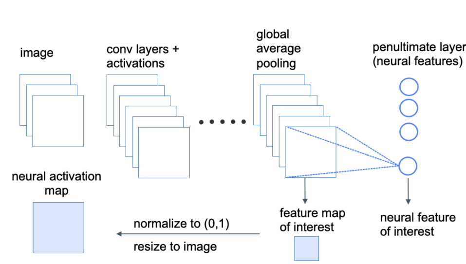
Figure 9: Figure describing the Neural Activation Map generation procedure. To obtain the neural activation map for feature $j$, we select the feature map from the output of the tensor of the previous layer (i.e the layer before the global average pooling operation). Next, we simply normalize the feature map between 0 and 1 and resize the feature map to match the image size, giving the neural activation map. This figure is from Singla & Feizi (2022) and included here for completeness.

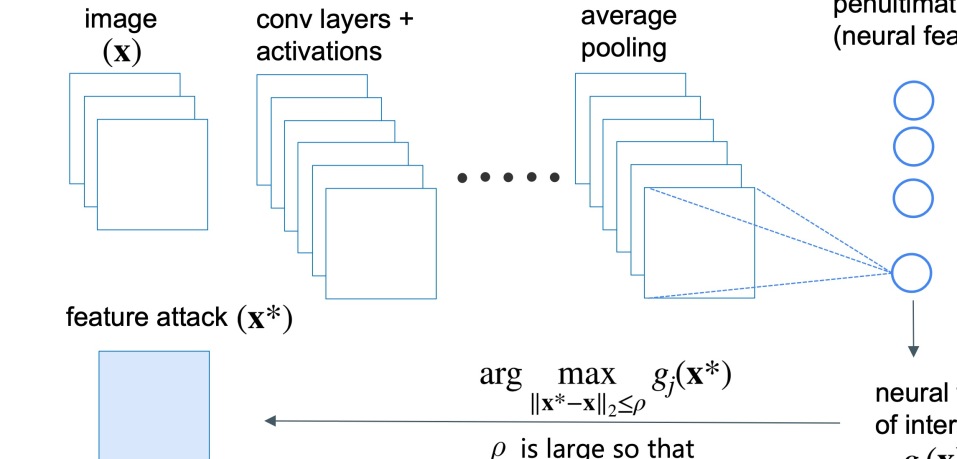
Figure 10: Figure illustrating the feature attack procedure. We select the feature we are interested in and simply optimize the image to maximize its value to generate the visualization. $\rho$ is a hyperparameter used to control the amount of change allowed in the image. For optimization, we use gradient ascent with step size = $40$, number of iterations = $25$ and $\rho$ = $500$. This figure is from Singla & Feizi (2022) and included here for completeness.

Appendix E Mechanical Turk study for discovering spurious features

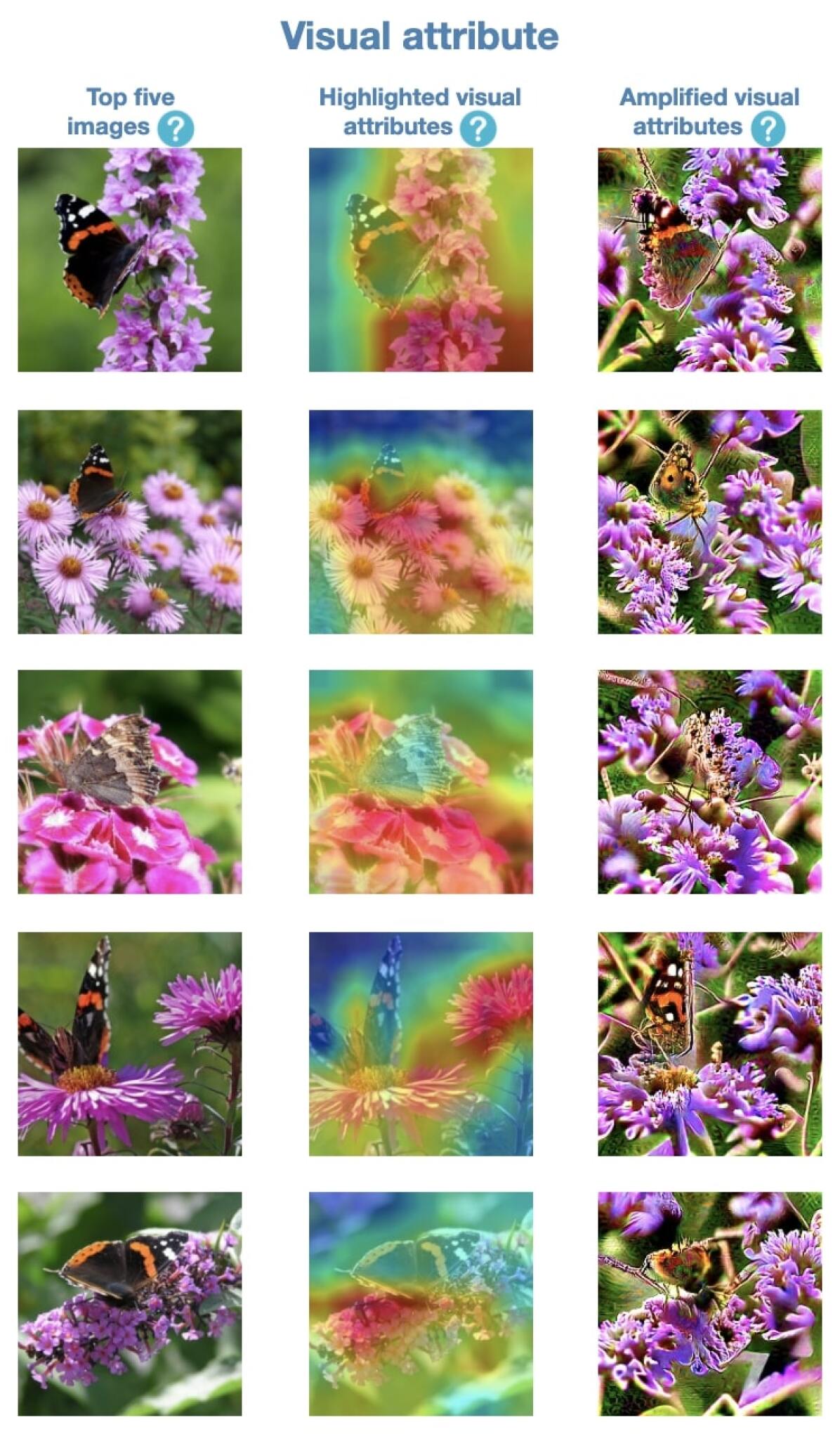
(a) Visual attribute

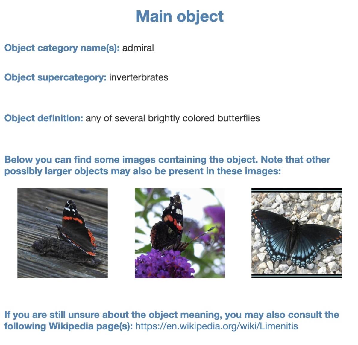
(b) Main object

(c) Questionnaire

Figure 11: Mechanical Turk study for discovering spurious features. This figure is from Singla & Feizi (2022) and included here for completeness.

The design for the Mechanical Turk study is shown in Figure 11. The left panel visualizing the neuron is shown in Figure 11(a). The right panel describing the object class is shown in Figure 11(b). The questionnaire is shown in Figure 11(c). We ask the workers to determine whether they think the visual attribute (given on the left) is a part of the main object (given on the right), some separate object or the background of the main object. We also ask the workers to provide reasons for their answers and rate their confidence on a likert scale from $1$ to $5$. The visualizations for which majority of workers selected either background or separate object as the answer were deemed to be spurious. Workers were paid $$0.1$ per HIT, with an average salary of $\$8$ per hour. In total, we had $137$ unique workers, each completing $140.15$ tasks (on average).

Appendix F Mechanical Turk study for validating heatmaps

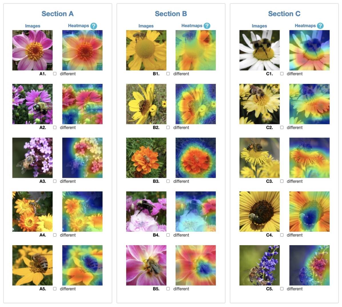
(a) Heatmaps highlighting the visual attributes

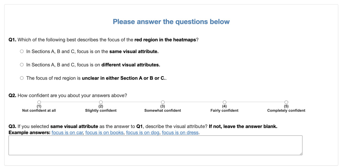
(b) Questionnaire

Figure 12: Mechanical Turk study for validating heatmaps

The design for the Mechanical Turk study is shown in Figure 12. The three panels showing heatmaps for different images from a class are shown in Figure 12(a). The questionnaire is shown in Figure 12(b). For each heatmap, workers were asked to determine if the highlighted attribute looked different from at least $3$ other heatmaps in the same panel. We also ask the workers to determine whether they think the focus of the heatmap is on the same object (in the three panels), different objects or whether they think the visualization in any of the panels is unclear. Same as in the previous study (Section E), we ask the workers to provide reasons for their answers and rate their confidence on a likert scale from $1$ to $5$. The visualizations for which at least $4$ workers selected same as the answer and for which at least $4$ workers did not select ”different” as the answer for all $15$ heatmaps were deemed to be validated i.e for this subset of $260$ images, we assume that the neural activation maps focus on the same visual attribute.

Appendix G Summary of the dataset validated using Mechanical Turk study in Section 4.2

Using the Mechanical Turk study in Section 4.2, for $4216$ (out of $4370$) core pairs i.e. (class=$i$, feature=$j$) pairs where $j$ is core for $i$, we validate that NAMs for the top-$260$ images indeed focus on the desired visual attribute. This directly results in $4216\times 260=1,096,160$ validated core masks.

Similarly, by taking the union of images in the sets $\mathcal{D}(i,j)$, again where $j$ is core for $i$ and (class=$i$, feature=$j$) is among the $4216$ validated pairs, we obtain $565,950$ unique images.

Appendix H Details on Relative Core Sensitivity

In this work, we use a novel metric to facilitate comparisons of core and spurious accuracies across a diverse set of models. Specifically, relative core sensitivity ($\mathrm{RCS}$) is designed to address the potential lurking variable of general noise robustness. For example, a model that is generally very robust to noise will see small degradation due to noise anywhere. Thus, the absolute difference between core and spurious accuracy will be small, regardless of the relative model sensitivity to either region. To normalize against this limitation, we scale the absolute gap by the total possible gap (made precise below).

We note that the metric Relative Core Sensitivity ($\mathrm{RCS}$) adapted here is same as the metric called Relative Foreground Sensitivity ($\mathrm{RFS}$) in Moayeri et al. (2022). We include two detailed derivations (one inspired from the original geometric derivation in Moayeri et al. (2022), and a new algebraic derivation) here for brevity.

H.1 Algebraic Derivation

Consider a model with core and spurious accuracies $\mathrm{acc^{(\mathcal{C})}},\mathrm{acc^{(\mathcal{S})}}$ respectively. We define $\bar{a}=\frac{(\mathrm{acc^{(\mathcal{C})}}+\mathrm{acc^{(\mathcal{S})}})}{2}$, and use $\bar{a}$ as a proxy for general noise robustness. The gap between $\mathrm{acc^{(\mathcal{C})}}$ and $\mathrm{acc^{(\mathcal{S})}}$ reflects sensitivity to noise in the non-core regions relative to core regions.

We seek to compute the maximum gap between $\mathrm{acc^{(\mathcal{C})}}$ and $\mathrm{acc^{(\mathcal{S})}}$ for a fixed general noise robustness of $\bar{a}$. The arguments maximizing the linear objective $\mathrm{acc^{(\mathcal{C})}}-\mathrm{acc^{(\mathcal{S})}}$ will occur at the boundary of the feasible region. There are two non-trivial cases to compare (the gap is obviously not maximized if $\mathrm{acc^{(\mathcal{C})}}\leq\mathrm{acc^{(\mathcal{S})}}$ so we ignore these cases):

• The maximum gap occurs when $\mathrm{acc^{(\mathcal{C})}}=1$. Thus, $\mathrm{acc^{(\mathcal{S})}}=2\bar{a}-1$, yielding a gap of $\mathrm{acc^{(\mathcal{C})}}-\mathrm{acc^{(\mathcal{S})}}=2(1-\bar{a})$.

• The maximum gap occurs when $\mathrm{acc^{(\mathcal{S})}}=0$. Thus, $\mathrm{acc^{(\mathcal{C})}}=2\bar{a}$, yielding a gap of $\mathrm{acc^{(\mathcal{C})}}-\mathrm{acc^{(\mathcal{S})}}=2\bar{a}$.

However, notice that the feasability of the above cases is contingent on $\bar{a}$. Specifically, $\mathrm{acc^{(\mathcal{C})}}$ can only be $1$ if $\bar{a}\geq 0.5$, and $\mathrm{acc^{(\mathcal{S})}}$ can only be $0$ if $\bar{a}\leq 0.5$. Thus, as a piecewise function with respect to $\bar{a}$, the maximum gap is $2\bar{a}$ for $\bar{a}\leq 0.5$ and $2(1-\bar{a})$ for $\bar{a}\geq 0.5$. Now, observe that this piecewise definition can be consolidated as $2\min(\bar{a},1-\bar{a})$.

Hence, defining $\mathrm{RCS}$ to be the ratio of the absolute gap between core and spurious accuracy, and the total possible gap for any model with general noise robustness of $\bar{a}$, yields the original formula $\mathrm{RCS}=\frac{\mathrm{acc^{(\mathcal{C})}}-\mathrm{acc^{(\mathcal{S})}}}{2\min(\bar{a},1-\bar{a})}$.

H.2 Geometric Derivation

$\mathrm{RCS}$ can also be viewed geometrically as the ratio of the distance of point $(\mathrm{acc^{(\mathcal{S})}},\mathrm{acc^{(\mathcal{C})}})$ above the diagonal over the maximum distance from the diagonal for models with fixed general noise robustness $\bar{a}$.

First, observe the distance of $(\mathrm{acc^{(\mathcal{S})}},\mathrm{acc^{(\mathcal{C})}})$ from the diagonal is given by the distance between the point and $(\bar{a},\bar{a})$, yielding:

$$\text{Distance to Diagonal}=\sqrt{2}(\bar{a}-\mathrm{acc^{(\mathcal{S})}})=\frac{\sqrt{2}(\mathrm{acc^{(\mathcal{C})}}-\mathrm{acc^{(\mathcal{S})}})}{2}$$

assuming that $\mathrm{acc^{(\mathcal{C})}}>\mathrm{acc^{(\mathcal{S})}}$ (though otherwise the sign would simply be flipped).

The maximum distance from the diagonal is constrained by the fact that $0\leq\mathrm{acc^{(\mathcal{C})}},\mathrm{acc^{(\mathcal{S})}}\leq 1$. Because $\bar{a}$ is fixed, we necessarily lie on the line $\mathrm{acc^{(\mathcal{C})}}=2\bar{a}-\mathrm{acc^{(\mathcal{S})}}$. Notice that when $\bar{a}\leq 0.5$, we intersect the boundary on the $y$-axis, at point $(0,2\bar{a})$. When $\bar{a}\geq 0.5$, we intersect the boundary defined by $y=1$, at the point $(1-2\bar{a},1)$. The corresponding maximum distances are then:

$$\text{Max Distance to Diagonal}=\sqrt{2}\bar{a}\;\text{ for }\;\bar{a}\leq 0.5,\text{ and }\sqrt{2}(1-\bar{a})\;\text{ for }\;\bar{a}\geq 0.5$$

As in the algebraic derivation, the piecewise formula can be resolved as $\sqrt{2}\min(\bar{a},1-\bar{a})$. Therefore, in the final ratio of distance of $(\mathrm{acc^{(\mathcal{S})}},\mathrm{acc^{(\mathcal{C})}})$ to diagonal over maximum distance to diagonal for fixed $\bar{a}$, the $\sqrt{2}$ terms cancel, yielding the formula for $\mathrm{RCS}$. For a pictographic geometric derivation, we refer readers to Moayeri et al. (2022).

Appendix I Novel Contributions compared to Previous Work

Certain aspects of our analysis are similar to previous work. Namely, the $\mathrm{RCS}$ metric is adapted from the relative foreground sensitivity metric of Moayeri et al. (2022), and both Moayeri et al. (2022) and Singla & Feizi (2022) conduct noise-based analyses to discern model sensitivity to image regions. Further, some of our observations on pretrained models were also noted in Moayeri et al. (2022) (i.e. lower sensitivity to core/foreground regions in transformers and adversarial trained Resnets, relative to Resnets). We acknowledge the inspiration taken from these efforts, and highlight two key distinguishing aspects of our work that we believe significantly add to the prior findings.

The first is scale, in both data and models: our evaluation includes $226k$ images from $985$ classes, compared to $5k$ from $20$ classes (organized into ten subsets called RIVAL$10$) in Moayeri et al. (2022), and $52k$ from $232$ classes in Singla & Feizi (2022); we evaluate $42$ models, compared to $17$ in Moayeri et al. (2022) and $4$ in Singla & Feizi (2022).

The second is that evaluating $\mathrm{RCS}$ on the test set of Salient Imagenet-1M can be done without making any changes to pretrained models, where as Moayeri et al. (2022) require models to be finetuned on the ten class subset of images they consider. While finetuning is a standard procedure, it changes the weights of neural features used to perform classification, which may introduce biases. Moreover, certain core features may be discarded when the classification task is simplified to the much coarser labels of RIVAL$10$. The evaluation in Singla & Feizi (2022) does not attempt to control for varying noise robustness, as models are not compared to one another directly.

Thus, we believe the findings of our experiments, due to the scale and lack of modifying pretrained models, may be empirically stronger than those of Moayeri et al. (2022). Nonetheless, we find it encouraging that we corroborate the findings of Moayeri et al. (2022) on a separate, larger dataset.

Appendix J Using data augmentation with Salient Imagenet-1M

J.1 Training Details for CoRM Models

We follow the fast training procedure for the baseline in Wong et al. (2020). Cyclic learning rates are applied from $0.1$ to $0.004$ for an SGD optimizer over 15 epochs. The only augmentation is to resize and center crop images to $224\times 224$. We discuss this choice below.

J.2 On Augmentation for Salient Imagenet-1M

Random cropping, a common augmentation technique, was not directly possible for the Salient ImageNet-1M version used in this work, as the masks were obtained for images after undergoing the standard ImageNet test transformations of resizing and taking a square center crop. However, there are multiple approaches for incorporating augmentation going forward.

First, one can generate the core masks by generating NAMs on the fly using the same robust model (used in this work for generating the NAMs for Salient Imagenet-1M) during training. That is, after performing any augmentation on the original image, one can compute NAMs for the relevant features on the augmented image, and use these directly as done in this work.

Second, one can precompute NAMs for all original images. This would require computing NAMs using training images that have been resized such that the shorter side is $224$. Then during training, the same random cropping transformation can be applied to the image and the mask to obtain the masks for the relevant core/non-core regions.

Thus, while augmentation was not used in this work, it is certainly feasible for Salient Imagenet-1M and will be explored in future works.

Appendix K Examples of spurious features

For each (class=$i$, feature=$j$) pair where $j$ is known to be spurious for the class $i$, we analyze the sensitivity of various standard (non-robust) trained models: Resnet-50, Efficientnet-B7, CLIP VIT-B32, VIT-B32 to different spurious features.

We first compute the clean accuracy for the set $\mathcal{D}(i,j)$ for each model (called initial in the the figure captions below). Next, for each image and spurious mask in $\mathcal{D}(i,j)$, i.e. $\mathbf{x},\mathbf{s}\in\mathcal{D}(i,j)$, we compute $\mathbf{x}^{*}=\mathbf{x}+\sigma\left(\mathbf{s}\odot\mathbf{z}\right)$ where $\mathbf{z}\sim\mathcal{N}\left(\boldsymbol{0},\mathbf{I}\right)$. Next, we compute the accuracy for each model using these noisy images and the drop in model accuracy (called accuracy drop in the figure captions below). We use $\sigma=0.25$.

K.1 Background spurious features

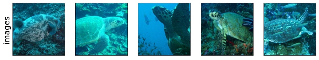
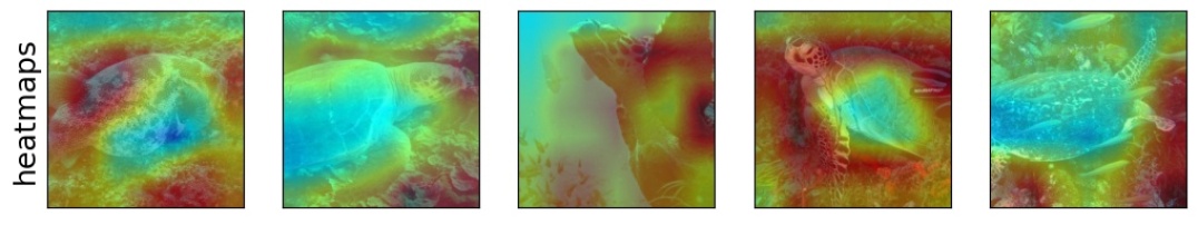
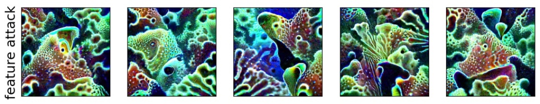
Figure 13: Visualization of feature 981 for class loggerhead (class index: 33).
For Resnet-50, accuracy drop: -73.846% (initial: 96.923%). For Efficientnet-B7, accuracy drop: -35.385% (initial: 89.231%).
For CLIP VIT-B32, accuracy drop: -53.846% (initial: 84.615%). For VIT-B32, accuracy drop: -30.769% (initial: 76.923%).

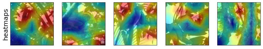
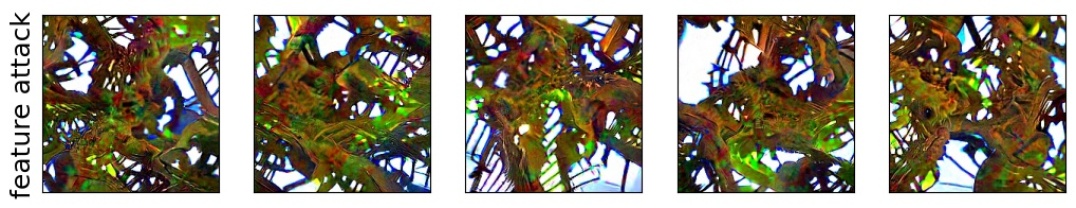
Figure 14: Visualization of feature 1199 for class three toed sloth (class index: 364).
For Resnet-50, accuracy drop: -64.615% (initial: 96.923%). For Efficientnet-B7, accuracy drop: -24.615% (initial: 93.846%).
For CLIP VIT-B32, accuracy drop: -67.692% (initial: 67.692%). For VIT-B32, accuracy drop: -4.615% (initial: 87.692%).

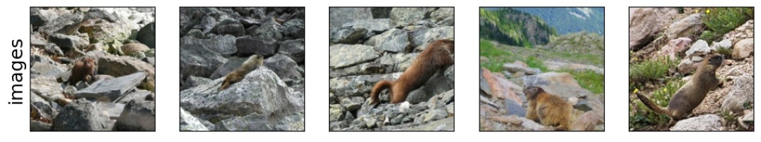
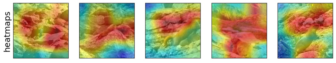
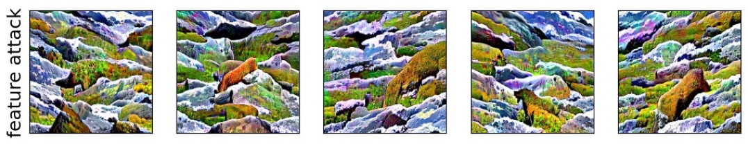
Figure 15: Visualization of feature 820 for class marmot (class index: 336).
For Resnet-50, accuracy drop: -64.616% (initial: 95.385%). For Efficientnet-B7, accuracy drop: -24.616% (initial: 86.154%).
For CLIP VIT-B32, accuracy drop: -47.693% (initial: 89.231%). For VIT-B32, accuracy drop: -40.0% (initial: 86.154%).

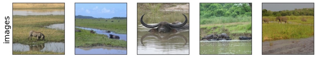
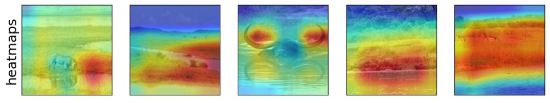
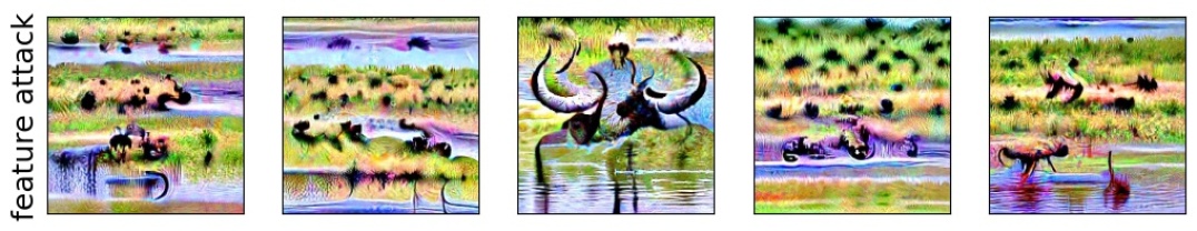
Figure 16: Visualization of feature 1127 for class water buffalo (class index: 346).
For Resnet-50, accuracy drop: -58.461% (initial: 84.615%). For Efficientnet-B7, accuracy drop: -44.615% (initial: 87.692%).
For CLIP VIT-B32, accuracy drop: -43.076% (initial: 81.538%). For VIT-B32, accuracy drop: -41.538% (initial: 90.769%).

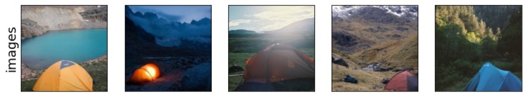
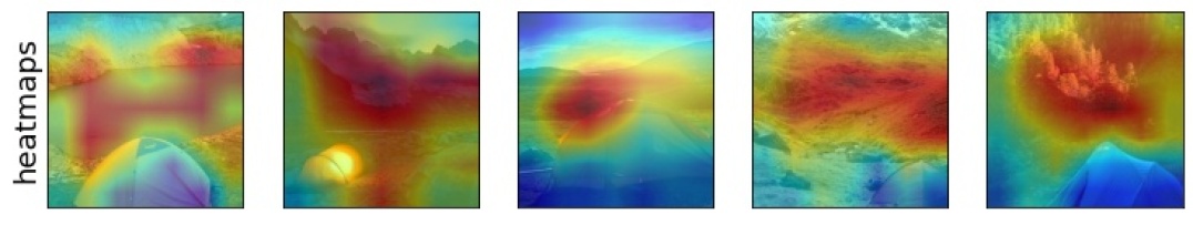
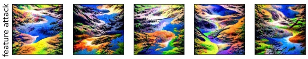
Figure 17: Visualization of feature 1239 for class mountain tent (class index: 672).
For Resnet-50, accuracy drop: -47.692% (initial: 96.923%). For Efficientnet-B7, accuracy drop: -10.77% (initial: 95.385%).
For CLIP VIT-B32, accuracy drop: -75.384% (initial: 87.692%). For VIT-B32, accuracy drop: -20.0% (initial: 96.923%).

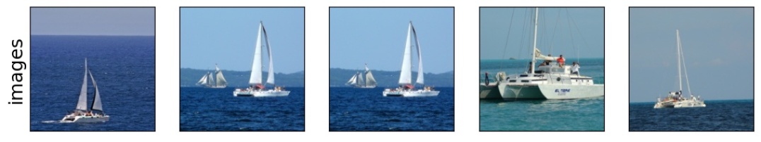
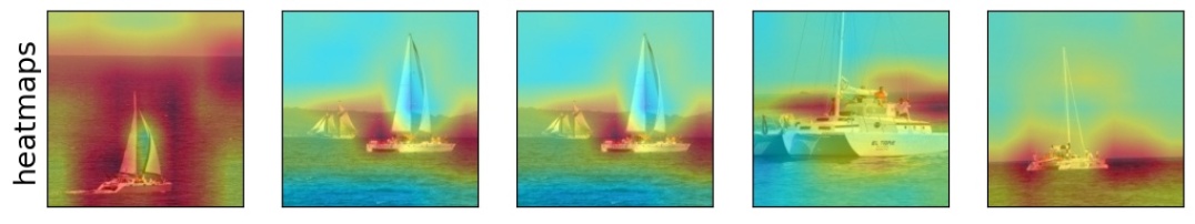
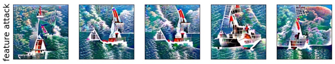
Figure 18: Visualization of feature 961 for class catamaran (class index: 484).
For Resnet-50, accuracy drop: -50.769% (initial: 93.846%). For Efficientnet-B7, accuracy drop: -20.0% (initial: 95.385%).
For CLIP VIT-B32, accuracy drop: -46.154% (initial: 89.231%). For VIT-B32, accuracy drop: -9.231% (initial: 93.846%).

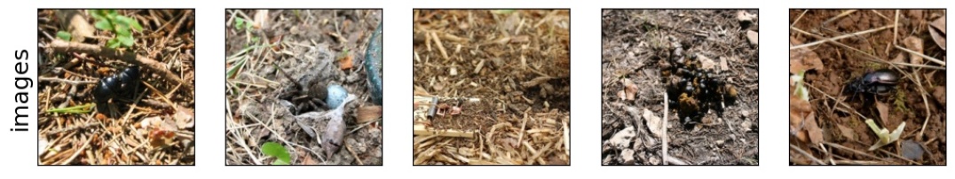
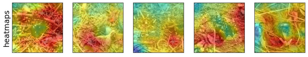
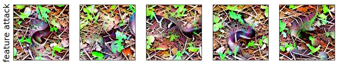
Figure 19: Visualization of feature 880 for class dung beetle (class index: 305).
For Resnet-50, accuracy drop: -50.77% (initial: 98.462%). For Efficientnet-B7, accuracy drop: -6.154% (initial: 98.462%).
For CLIP VIT-B32, accuracy drop: -52.308% (initial: 80.0%). For VIT-B32, accuracy drop: -13.846% (initial: 90.769%).

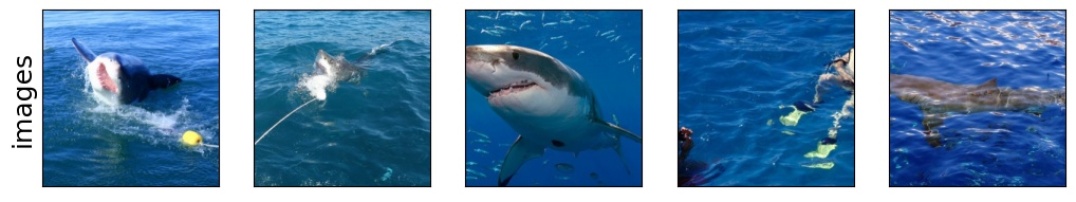
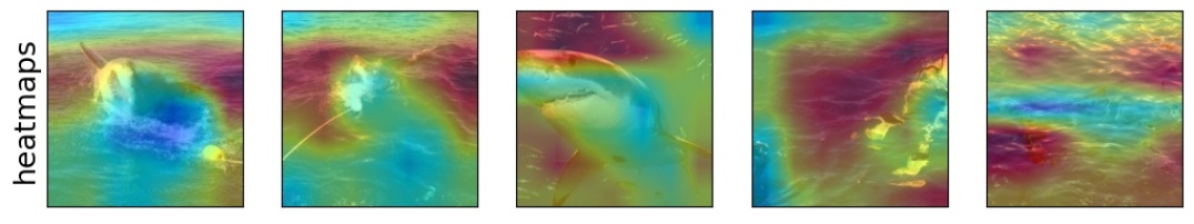
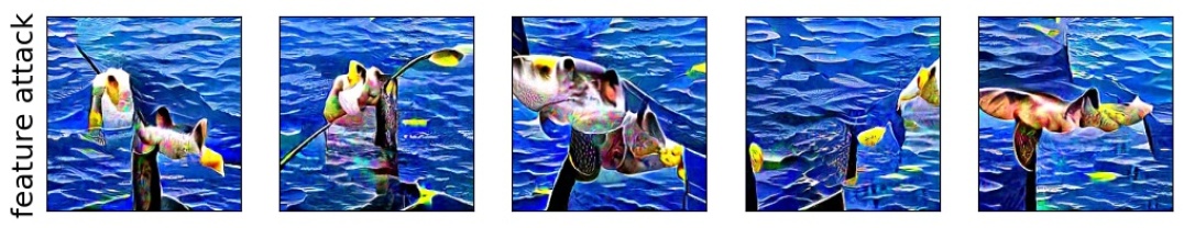
Figure 20: Visualization of feature 1697 for class great white shark (class index: 2).
For Resnet-50, accuracy drop: -44.615% (initial: 90.769%). For Efficientnet-B7, accuracy drop: -38.461% (initial: 87.692%).
For CLIP VIT-B32, accuracy drop: -26.154% (initial: 49.231%). For VIT-B32, accuracy drop: -23.077% (initial: 84.615%).

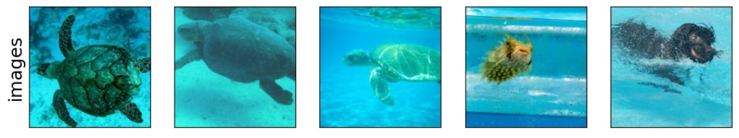
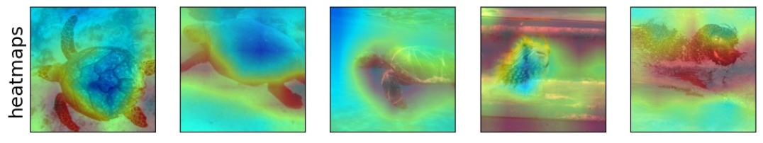
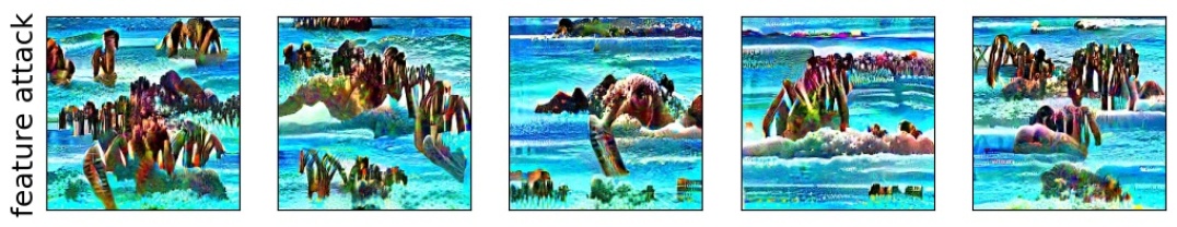
Figure 21: Visualization of feature 491 for class loggerhead (class index: 33).
For Resnet-50, accuracy drop: -78.462% (initial: 95.385%). For Efficientnet-B7, accuracy drop: -29.231% (initial: 89.231%).
For CLIP VIT-B32, accuracy drop: -35.384% (initial: 87.692%). For VIT-B32, accuracy drop: -21.539% (initial: 83.077%).

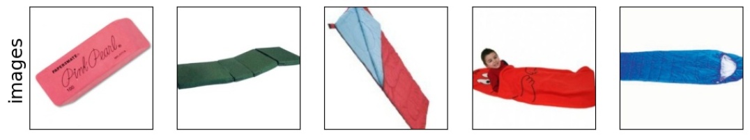
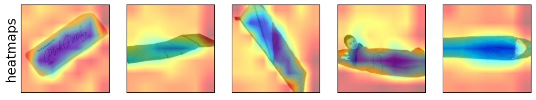
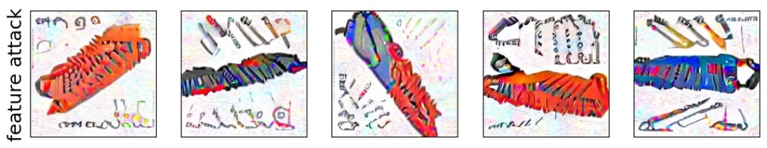
Figure 22: Visualization of feature 118 for class sleeping bag (class index: 797).
For Resnet-50, accuracy drop: -41.539% (initial: 98.462%). For Efficientnet-B7, accuracy drop: -20.0% (initial: 95.385%).
For CLIP VIT-B32, accuracy drop: -63.077% (initial: 78.462%). For VIT-B32, accuracy drop: -10.769% (initial: 84.615%).

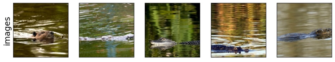
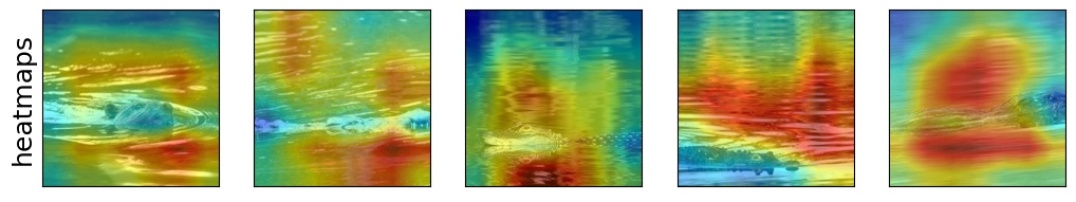
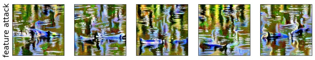
Figure 23: Visualization of feature 341 for class beaver (class index: 337).
For Resnet-50, accuracy drop: -43.077% (initial: 96.923%). For Efficientnet-B7, accuracy drop: -21.538% (initial: 96.923%).
For CLIP VIT-B32, accuracy drop: -35.385% (initial: 58.462%). For VIT-B32, accuracy drop: -12.308% (initial: 89.231%).

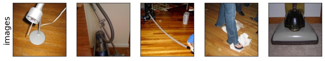
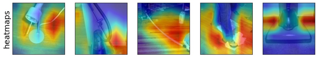
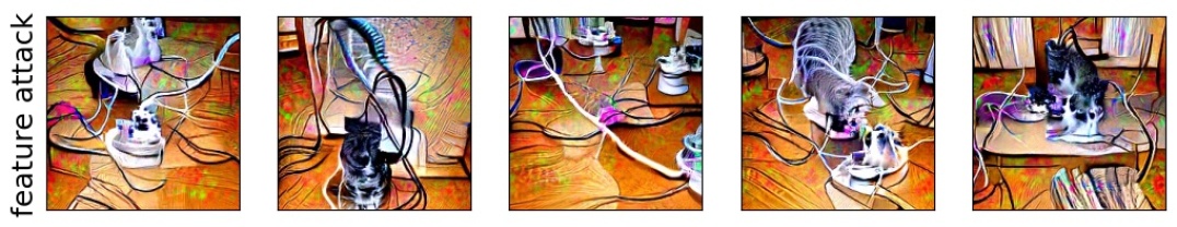
Figure 24: Visualization of feature 1291 for class vacuum (class index: 882).
For Resnet-50, accuracy drop: -29.231% (initial: 93.846%). For Efficientnet-B7, accuracy drop: -18.462% (initial: 86.154%).
For CLIP VIT-B32, accuracy drop: -44.615% (initial: 70.769%). For VIT-B32, accuracy drop: -26.154% (initial: 92.308%).

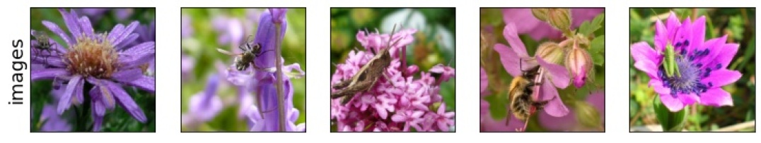
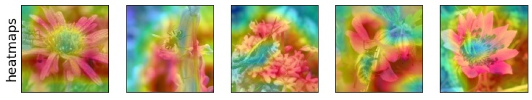
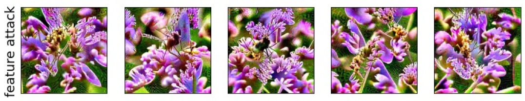
Figure 25: Visualization of feature 1797 for class bee (class index: 309).
For Resnet-50, accuracy drop: -40.0% (initial: 90.769%). For Efficientnet-B7, accuracy drop: -15.385% (initial: 89.231%).
For CLIP VIT-B32, accuracy drop: -36.923% (initial: 95.385%). For VIT-B32, accuracy drop: -3.077% (initial: 89.231%).

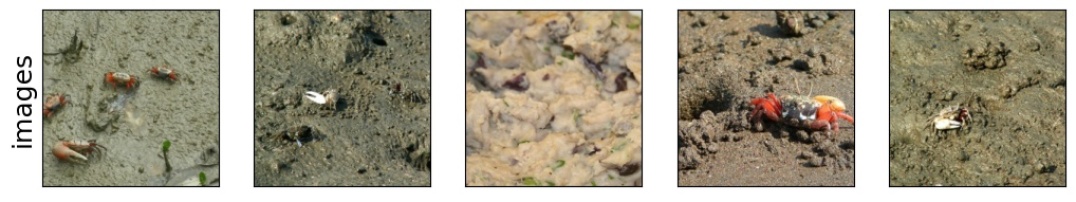
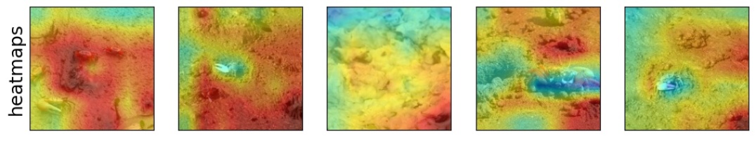
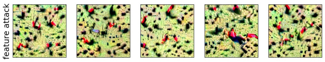
Figure 26: Visualization of feature 870 for class fiddler crab (class index: 120).
For Resnet-50, accuracy drop: -24.615% (initial: 100.0%). For Efficientnet-B7, accuracy drop: -18.462% (initial: 98.462%).
For CLIP VIT-B32, accuracy drop: -61.539% (initial: 89.231%). For VIT-B32, accuracy drop: -6.154% (initial: 95.385%).

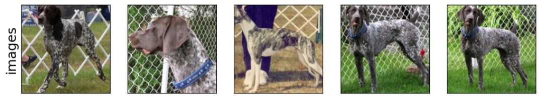
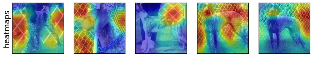
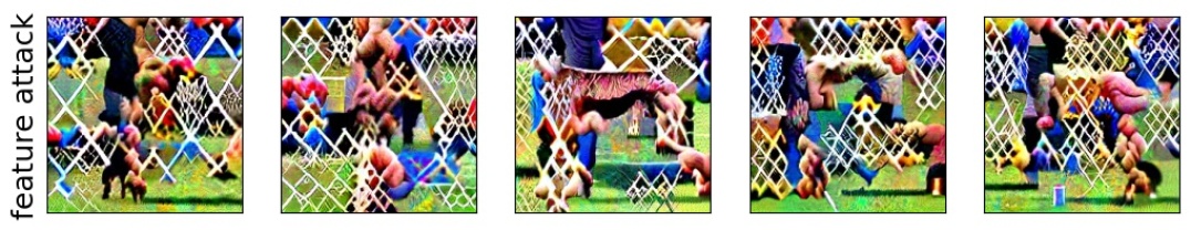
Figure 27: Visualization of feature 1856 for class german short haired pointer (class index: 210).
For Resnet-50, accuracy drop: -27.693% (initial: 95.385%). For Efficientnet-B7, accuracy drop: -3.077% (initial: 98.462%).
For CLIP VIT-B32, accuracy drop: -32.307% (initial: 81.538%). For VIT-B32, accuracy drop: -13.846% (initial: 92.308%).

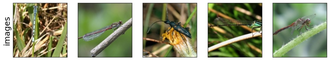
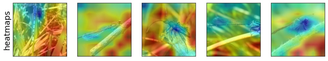
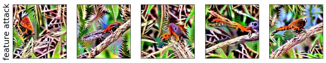
Figure 28: Visualization of feature 1556 for class damselfly (class index: 320).
For Resnet-50, accuracy drop: -30.77% (initial: 95.385%). For Efficientnet-B7, accuracy drop: -4.615% (initial: 96.923%).
For CLIP VIT-B32, accuracy drop: -44.615% (initial: 93.846%). For VIT-B32, accuracy drop: -10.769% (initial: 89.231%).

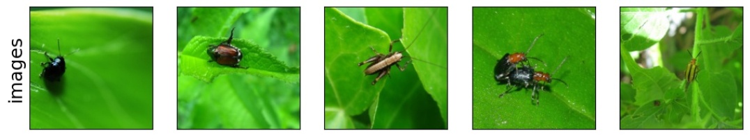
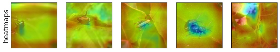
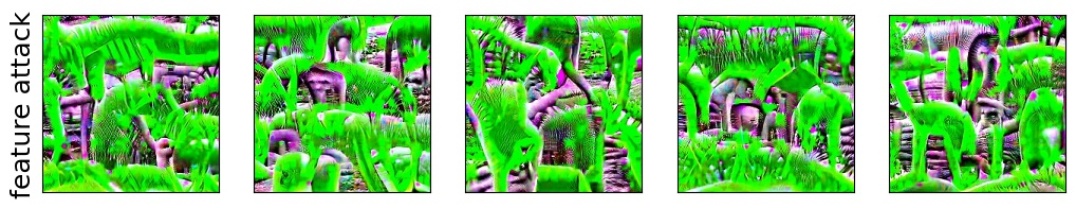
Figure 29: Visualization of feature 1994 for class leaf beetle (class index: 304).
For Resnet-50, accuracy drop: -41.539% (initial: 86.154%). For Efficientnet-B7, accuracy drop: -12.308% (initial: 75.385%).
For CLIP VIT-B32, accuracy drop: -40.0% (initial: 81.538%). For VIT-B32, accuracy drop: +0.0% (initial: 60.0%).

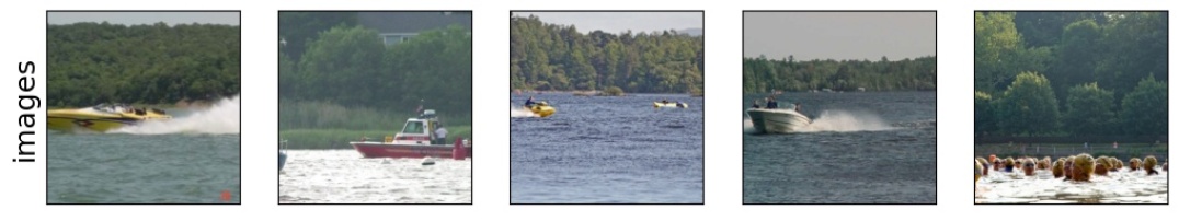
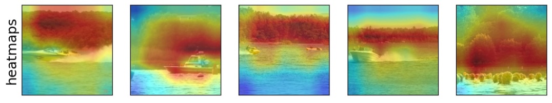
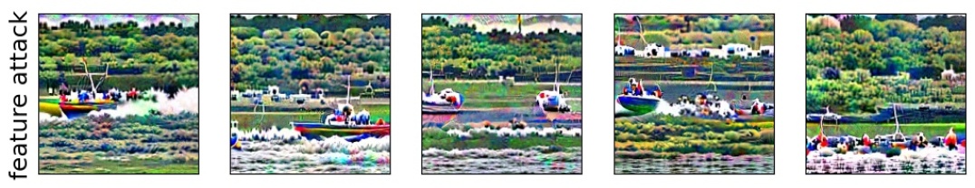
Figure 30: Visualization of feature 1901 for class speedboat (class index: 814).
For Resnet-50, accuracy drop: -56.924% (initial: 98.462%). For Efficientnet-B7, accuracy drop: -10.77% (initial: 98.462%).
For CLIP VIT-B32, accuracy drop: -24.616% (initial: 38.462%). For VIT-B32, accuracy drop: -13.846% (initial: 100.0%).

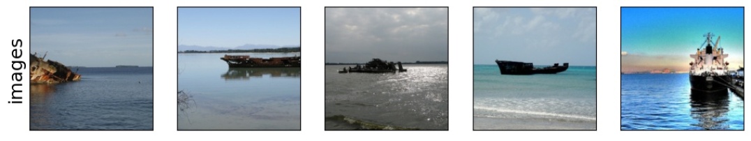
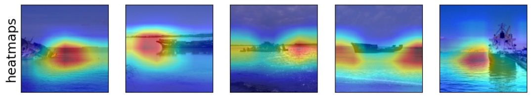
Figure 31: Visualization of feature 421 for class wreck (class index: 913).
For Resnet-50, accuracy drop: -26.154% (initial: 83.077%). For Efficientnet-B7, accuracy drop: -21.538% (initial: 84.615%).
For CLIP VIT-B32, accuracy drop: -35.385% (initial: 55.385%). For VIT-B32, accuracy drop: -18.461% (initial: 67.692%).

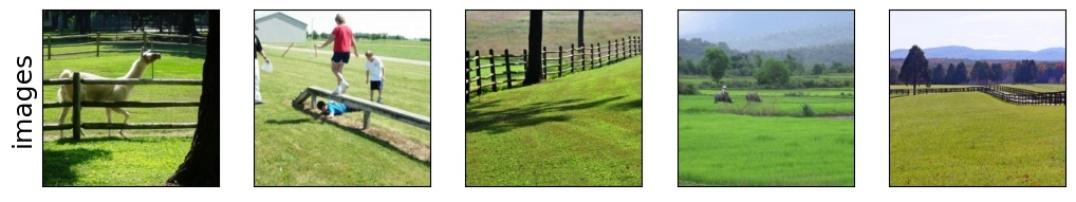
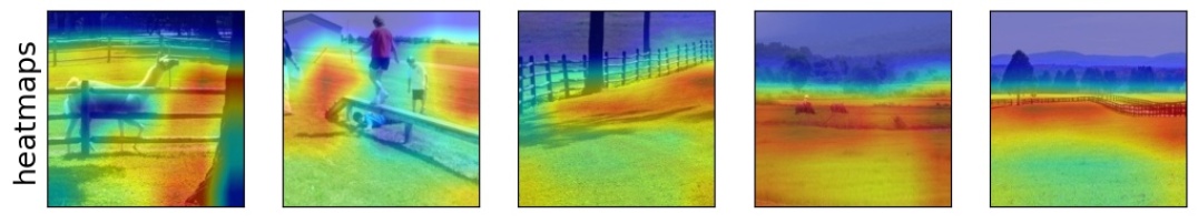
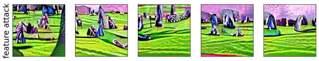
Figure 32: Visualization of feature 1050 for class worm fence (class index: 912).
For Resnet-50, accuracy drop: -26.154% (initial: 95.385%). For Efficientnet-B7, accuracy drop: -7.693% (initial: 95.385%).
For CLIP VIT-B32, accuracy drop: -38.461% (initial: 76.923%). For VIT-B32, accuracy drop: -6.154% (initial: 96.923%).

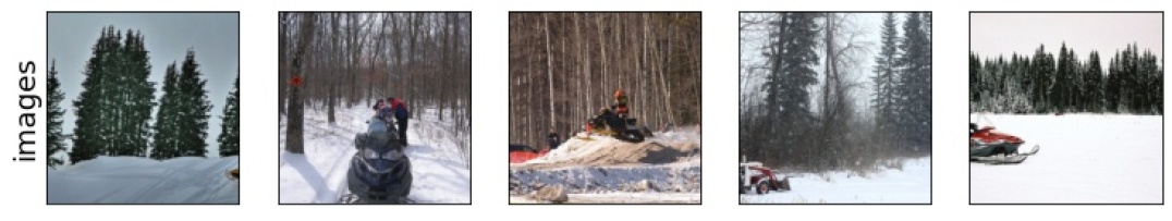
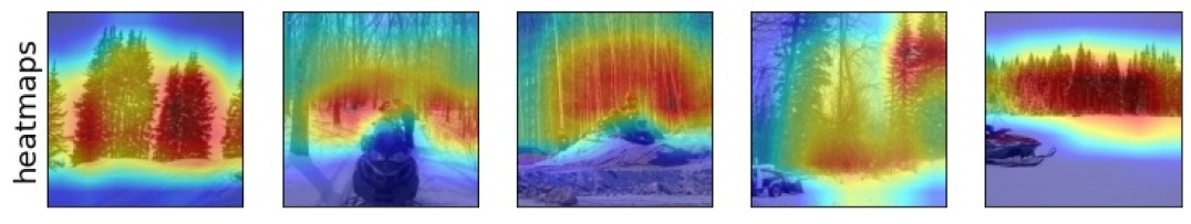
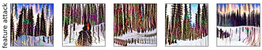
Figure 33: Visualization of feature 0 for class snowmobile (class index: 802).
For Resnet-50, accuracy drop: -21.538% (initial: 100.0%). For Efficientnet-B7, accuracy drop: -3.077% (initial: 98.462%).
For CLIP VIT-B32, accuracy drop: -27.693% (initial: 89.231%). For VIT-B32, accuracy drop: -10.769% (initial: 93.846%).

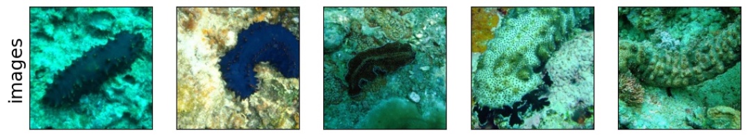
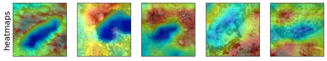
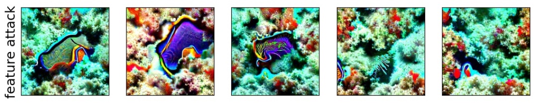
Figure 34: Visualization of feature 1753 for class sea cucumber (class index: 329).
For Resnet-50, accuracy drop: -20.0% (initial: 93.846%). For Efficientnet-B7, accuracy drop: -12.307% (initial: 87.692%).
For CLIP VIT-B32, accuracy drop: -58.462% (initial: 86.154%). For VIT-B32, accuracy drop: -1.539% (initial: 66.154%).

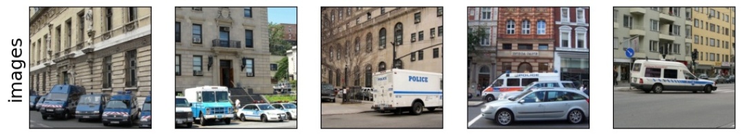
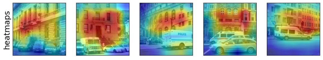
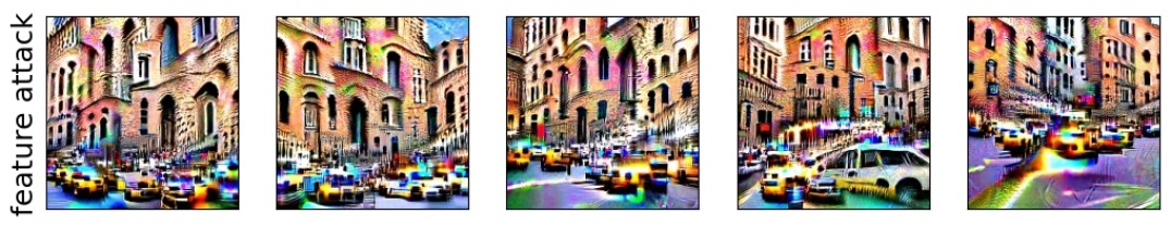
Figure 35: Visualization of feature 1026 for class police van (class index: 734).
For Resnet-50, accuracy drop: -44.616% (initial: 89.231%). For Efficientnet-B7, accuracy drop: -16.923% (initial: 87.692%).
For CLIP VIT-B32, accuracy drop: -3.077% (initial: 72.308%). For VIT-B32, accuracy drop: -13.847% (initial: 78.462%).

K.2 Foreground spurious features

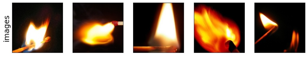
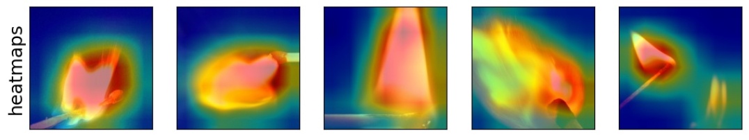
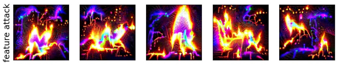
Figure 36: Visualization of feature 1986 for class matchstick (class index: 644).
For Resnet-50, accuracy drop: -43.077% (initial: 96.923%). For Efficientnet-B7, accuracy drop: -15.385% (initial: 98.462%).
For CLIP VIT-B32, accuracy drop: -44.616% (initial: 55.385%). For VIT-B32, accuracy drop: -4.616% (initial: 95.385%).

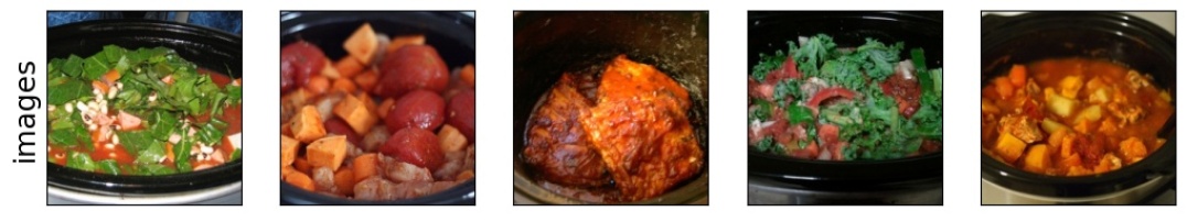
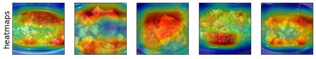
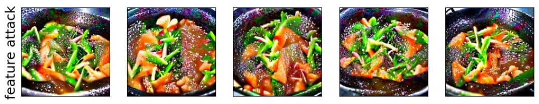
Figure 37: Visualization of feature 895 for class crock pot (class index: 521).
For Resnet-50, accuracy drop: -38.461% (initial: 67.692%). For Efficientnet-B7, accuracy drop: -13.846% (initial: 64.615%).
For CLIP VIT-B32, accuracy drop: -61.538% (initial: 67.692%). For VIT-B32, accuracy drop: -20.0% (initial: 81.538%).

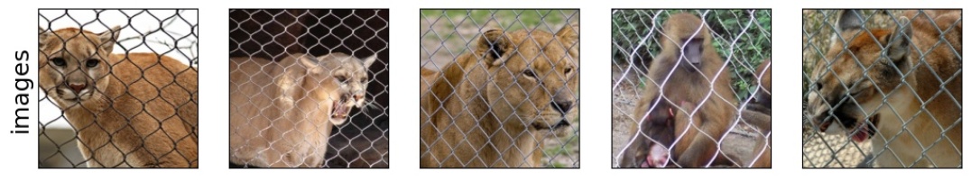
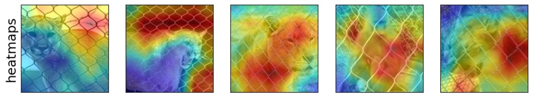
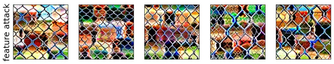
Figure 38: Visualization of feature 1401 for class cougar (class index: 286).
For Resnet-50, accuracy drop: -43.077% (initial: 96.923%). For Efficientnet-B7, accuracy drop: -7.692% (initial: 96.923%).
For CLIP VIT-B32, accuracy drop: -72.308% (initial: 83.077%). For VIT-B32, accuracy drop: -6.154% (initial: 92.308%).

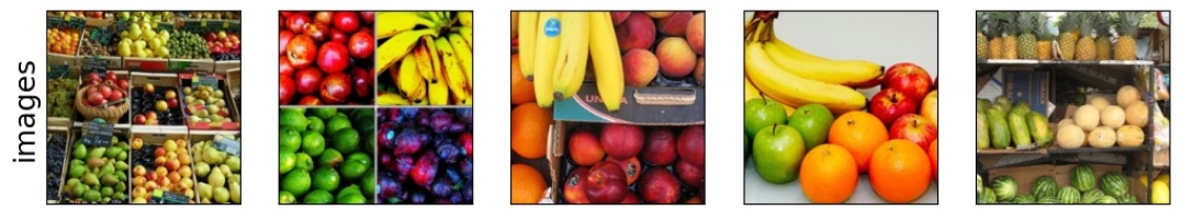
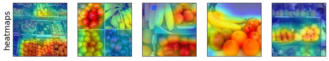
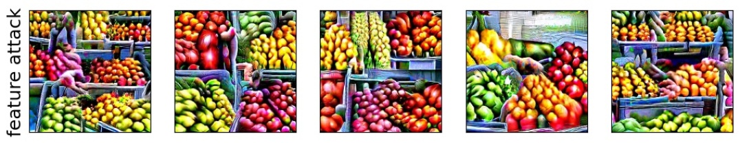
Figure 39: Visualization of feature 68 for class banana (class index: 954).
For Resnet-50, accuracy drop: -46.154% (initial: 89.231%). For Efficientnet-B7, accuracy drop: -18.462% (initial: 92.308%).
For CLIP VIT-B32, accuracy drop: -27.693% (initial: 52.308%). For VIT-B32, accuracy drop: -15.384% (initial: 81.538%).

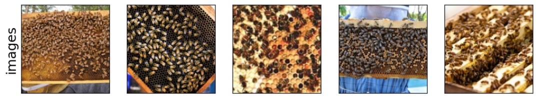
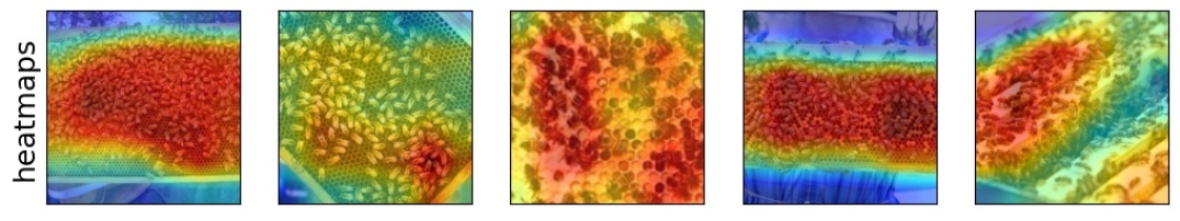
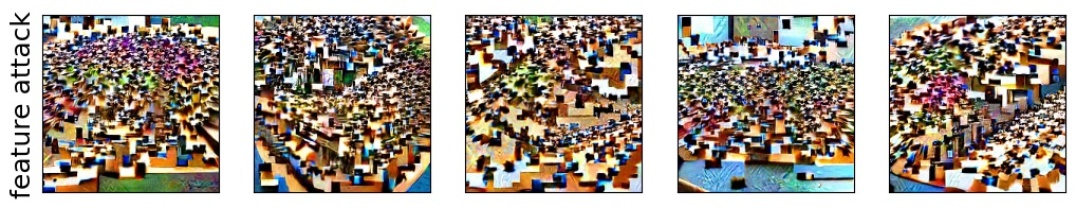
Figure 40: Visualization of feature 1849 for class apiary (class index: 410).
For Resnet-50, accuracy drop: -53.846% (initial: 87.692%). For Efficientnet-B7, accuracy drop: -26.153% (initial: 81.538%).
For CLIP VIT-B32, accuracy drop: -16.923% (initial: 61.538%). For VIT-B32, accuracy drop: -15.385% (initial: 46.154%).

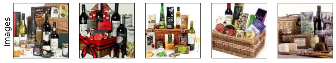
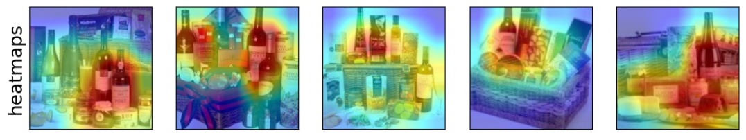
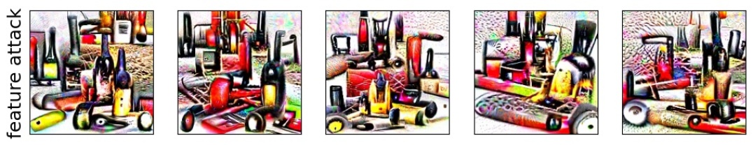
Figure 41: Visualization of feature 834 for class hamper (class index: 588).
For Resnet-50, accuracy drop: -56.923% (initial: 100.0%). For Efficientnet-B7, accuracy drop: -27.692% (initial: 100.0%).
For CLIP VIT-B32, accuracy drop: -7.692% (initial: 100.0%). For VIT-B32, accuracy drop: -10.769% (initial: 93.846%).

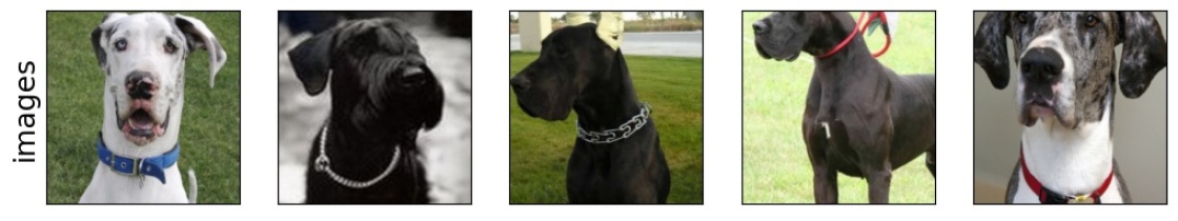
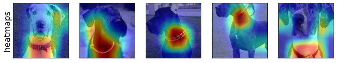
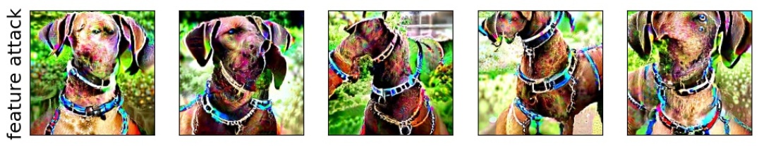
Figure 42: Visualization of feature 1634 for class great dane (class index: 246).
For Resnet-50, accuracy drop: -23.077% (initial: 95.385%). For Efficientnet-B7, accuracy drop: -13.846% (initial: 100.0%).
For CLIP VIT-B32, accuracy drop: -38.461% (initial: 41.538%). For VIT-B32, accuracy drop: -10.769% (initial: 90.769%).

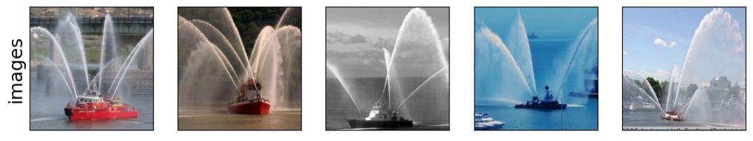
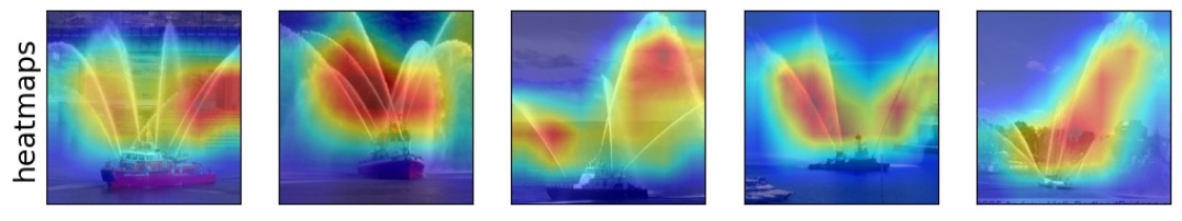
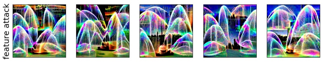
Figure 43: Visualization of feature 2010 for class fireboat (class index: 554).
For Resnet-50, accuracy drop: -33.846% (initial: 100.0%). For Efficientnet-B7, accuracy drop: +0.0% (initial: 100.0%).
For CLIP VIT-B32, accuracy drop: -36.923% (initial: 96.923%). For VIT-B32, accuracy drop: -3.077% (initial: 100.0%).

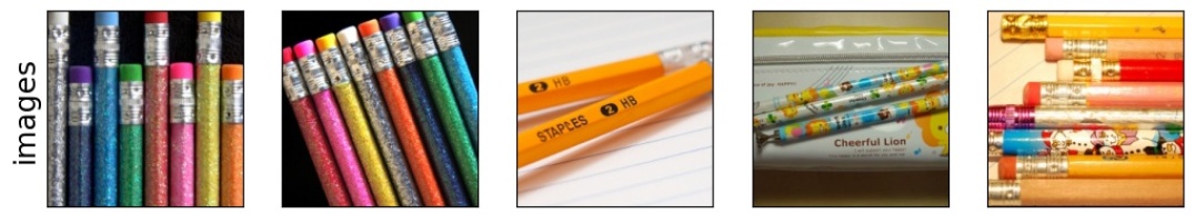
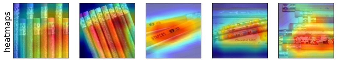
Figure 44: Visualization of feature 1052 for class rubber eraser (class index: 767).
For Resnet-50, accuracy drop: -47.692% (initial: 86.154%). For Efficientnet-B7, accuracy drop: -16.923% (initial: 92.308%).
For CLIP VIT-B32, accuracy drop: -4.615% (initial: 10.769%). For VIT-B32, accuracy drop: -18.462% (initial: 80.0%).

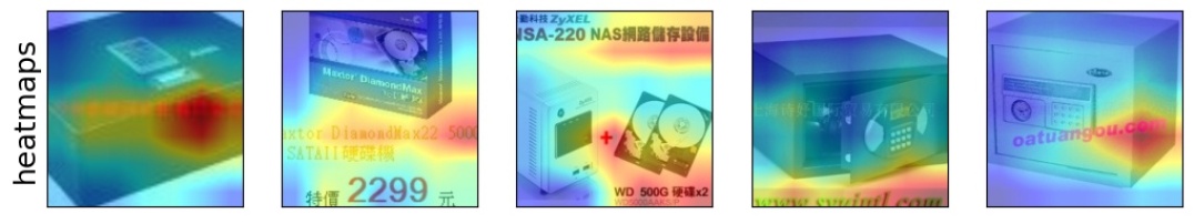
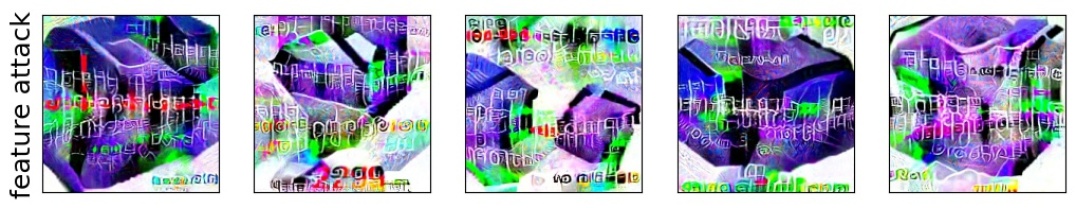
Figure 45: Visualization of feature 388 for class safe (class index: 771).
For Resnet-50, accuracy drop: -26.154% (initial: 89.231%). For Efficientnet-B7, accuracy drop: -6.154% (initial: 86.154%).
For CLIP VIT-B32, accuracy drop: -30.77% (initial: 38.462%). For VIT-B32, accuracy drop: -1.539% (initial: 83.077%).

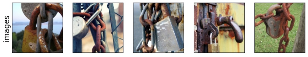
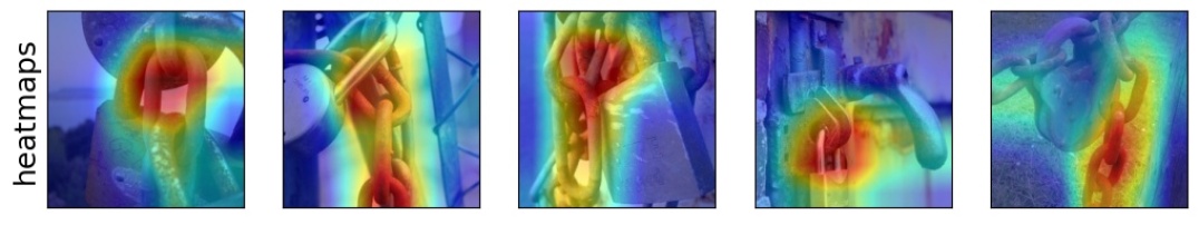
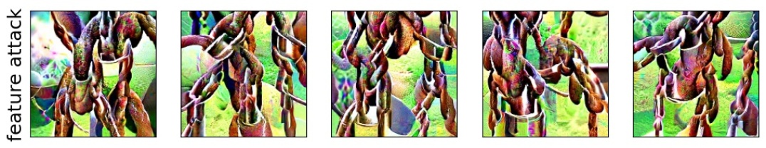
Figure 46: Visualization of feature 128 for class padlock (class index: 695).
For Resnet-50, accuracy drop: -12.307% (initial: 87.692%). For Efficientnet-B7, accuracy drop: -15.385% (initial: 95.385%).
For CLIP VIT-B32, accuracy drop: -63.077% (initial: 92.308%). For VIT-B32, accuracy drop: -4.616% (initial: 86.154%).

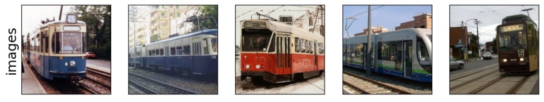
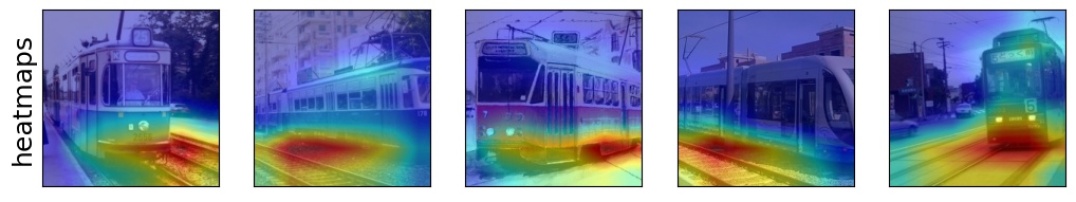
Figure 47: Visualization of feature 56 for class streetcar (class index: 829).
For Resnet-50, accuracy drop: -12.307% (initial: 87.692%). For Efficientnet-B7, accuracy drop: -15.384% (initial: 93.846%).
For CLIP VIT-B32, accuracy drop: -29.231% (initial: 92.308%). For VIT-B32, accuracy drop: -6.154% (initial: 93.846%).

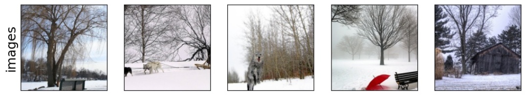
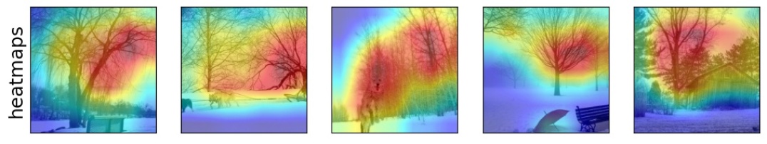
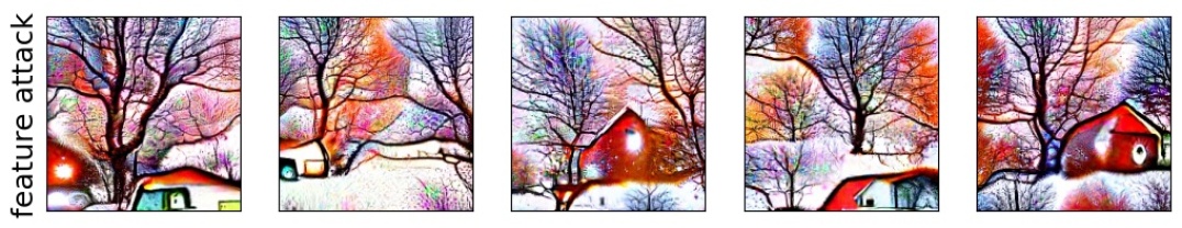
Figure 48: Visualization of feature 1623 for class snowplow (class index: 803).
For Resnet-50, accuracy drop: -18.461% (initial: 96.923%). For Efficientnet-B7, accuracy drop: -6.154% (initial: 95.385%).
For CLIP VIT-B32, accuracy drop: -38.461% (initial: 93.846%). For VIT-B32, accuracy drop: -4.615% (initial: 96.923%).

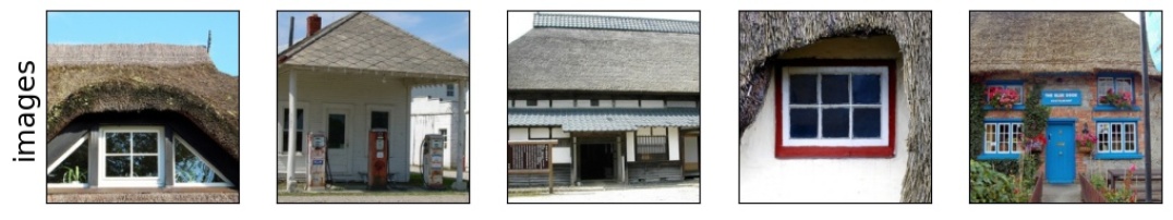
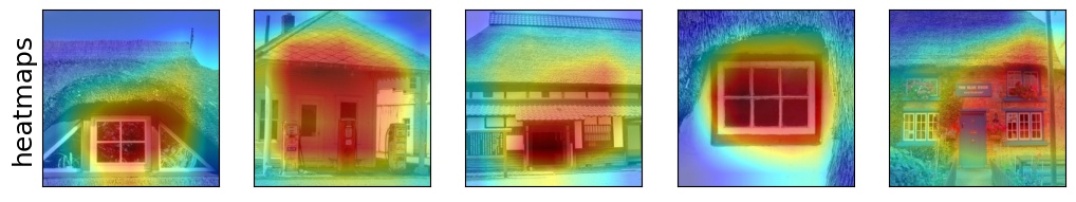
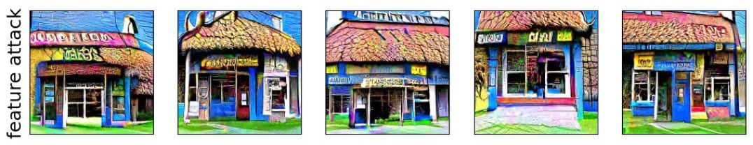
Figure 49: Visualization of feature 466 for class thatch (class index: 853).
For Resnet-50, accuracy drop: -13.846% (initial: 100.0%). For Efficientnet-B7, accuracy drop: -7.692% (initial: 100.0%).
For CLIP VIT-B32, accuracy drop: -15.385% (initial: 98.462%). For VIT-B32, accuracy drop: -4.615% (initial: 96.923%).

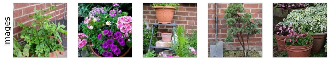
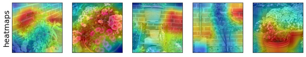
Figure 50: Visualization of feature 1829 for class pot (class index: 738).
For Resnet-50, accuracy drop: -35.385% (initial: 95.385%). For Efficientnet-B7, accuracy drop: -7.693% (initial: 92.308%).
For CLIP VIT-B32, accuracy drop: +1.538% (initial: 60.0%). For VIT-B32, accuracy drop: -12.308% (initial: 96.923%).

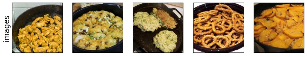
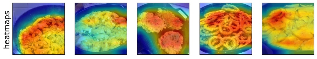
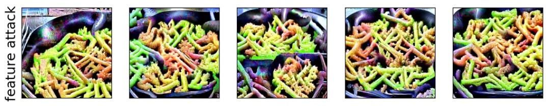
Figure 51: Visualization of feature 2000 for class frying pan (class index: 567).
For Resnet-50, accuracy drop: -9.23% (initial: 84.615%). For Efficientnet-B7, accuracy drop: -20.0% (initial: 72.308%).
For CLIP VIT-B32, accuracy drop: -10.77% (initial: 12.308%). For VIT-B32, accuracy drop: +3.077% (initial: 46.154%).

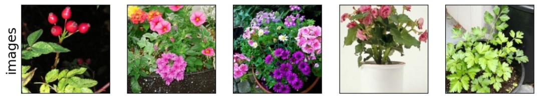
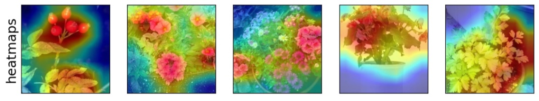
Figure 52: Visualization of feature 1392 for class pot (class index: 738).
For Resnet-50, accuracy drop: -41.538% (initial: 90.769%). For Efficientnet-B7, accuracy drop: -6.154% (initial: 93.846%).
For CLIP VIT-B32, accuracy drop: -12.308% (initial: 69.231%). For VIT-B32, accuracy drop: -6.154% (initial: 87.692%).

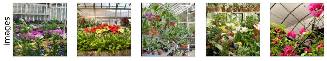
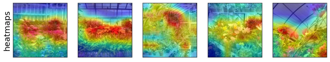
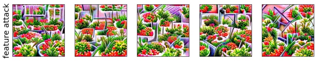
Figure 53: Visualization of feature 1933 for class greenhouse (class index: 580).
For Resnet-50, accuracy drop: -9.231% (initial: 93.846%). For Efficientnet-B7, accuracy drop: +0.0% (initial: 96.923%).
For CLIP VIT-B32, accuracy drop: -7.692% (initial: 90.769%). For VIT-B32, accuracy drop: -7.693% (initial: 89.231%).

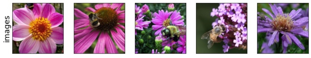
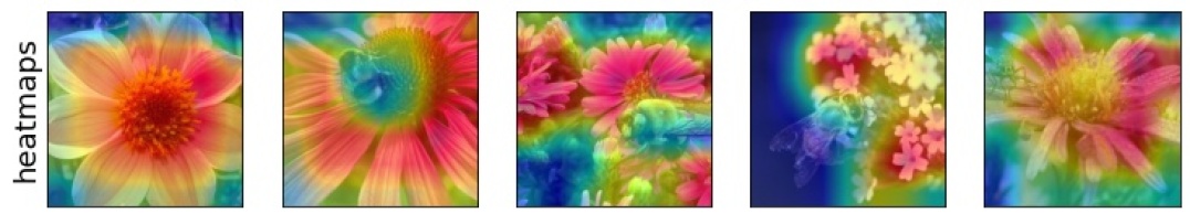
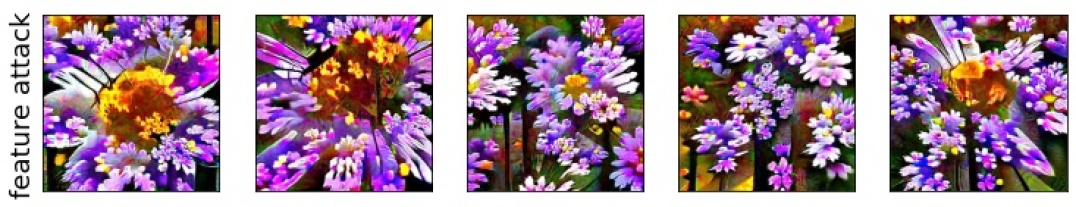
Figure 54: Visualization of feature 595 for class bee (class index: 309).
For Resnet-50, accuracy drop: -41.539% (initial: 86.154%). For Efficientnet-B7, accuracy drop: -21.538% (initial: 76.923%).
For CLIP VIT-B32, accuracy drop: -58.461% (initial: 93.846%). For VIT-B32, accuracy drop: -10.769% (initial: 86.154%).

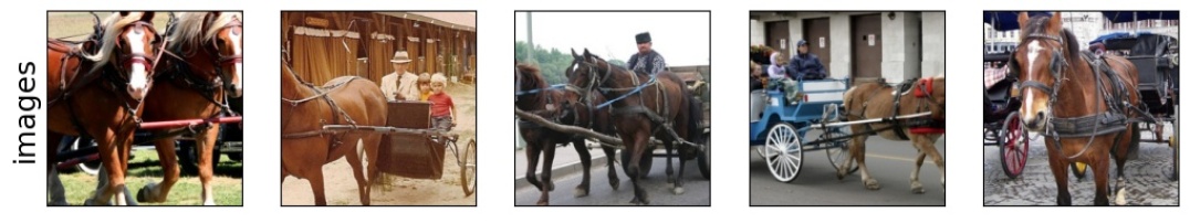
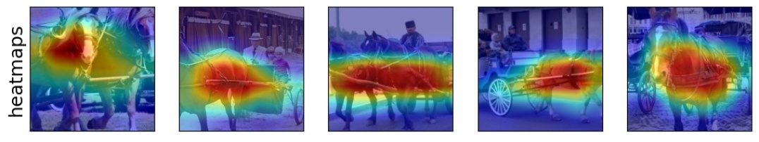
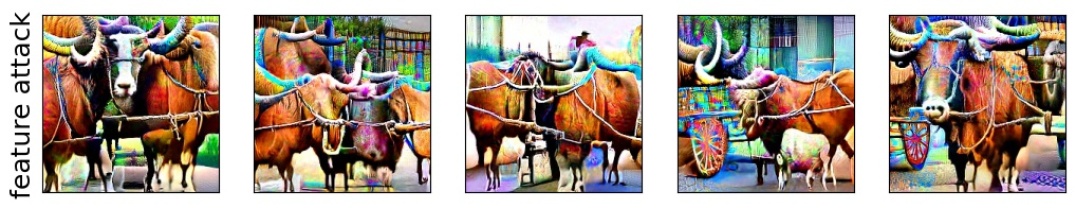
Figure 55: Visualization of feature 1526 for class horse cart (class index: 603).
For Resnet-50, accuracy drop: -3.077% (initial: 98.462%). For Efficientnet-B7, accuracy drop: -1.539% (initial: 98.462%).
For CLIP VIT-B32, accuracy drop: -24.615% (initial: 87.692%). For VIT-B32, accuracy drop: -9.231% (initial: 96.923%).

References

- Adebayo et al. (2018) Adebayo, J., Gilmer, J., Muelly, M., Goodfellow, I. J., Hardt, M., and Kim, B. Sanity checks for saliency maps. In NeurIPS, 2018.
- Ahuja et al. (2020) Ahuja, K., Shanmugam, K., Varshney, K., and Dhurandhar, A. Invariant risk minimization games. In III, H. D. and Singh, A. (eds.), Proceedings of the 37th International Conference on Machine Learning, volume 119 of Proceedings of Machine Learning Research, pp. 145–155. PMLR, 13–18 Jul 2020. URL https://proceedings.mlr.press/v119/ahuja20a.html.
- Ahuja et al. (2021) Ahuja, K., Wang, J., Dhurandhar, A., Shanmugam, K., and Varshney, K. R. Empirical or invariant risk minimization? a sample complexity perspective. In International Conference on Learning Representations, 2021. URL https://openreview.net/forum?id=jrA5GAccy_.
- Arjovsky et al. (2020) Arjovsky, M., Bottou, L., Gulrajani, I., and Lopez-Paz, D. Invariant risk minimization, 2020.
- Bagnell (2005) Bagnell, J. A. Robust supervised learning. In AAAI, 2005.
- Bau et al. (2020) Bau, D., Zhu, J.-Y., Strobelt, H., Lapedriza, A., Zhou, B., and Torralba, A. Understanding the role of individual units in a deep neural network. Proceedings of the National Academy of Sciences, 117(48):30071–30078, 2020. ISSN 0027-8424. doi: 10.1073/pnas.1907375117. URL https://www.pnas.org/content/117/48/30071.
- Beery et al. (2018) Beery, S., Horn, G. V., and Perona, P. Recognition in terra incognita. CoRR, abs/1807.04975, 2018. URL http://arxiv.org/abs/1807.04975.
- Bickel et al. (2009) Bickel, S., Brückner, M., and Scheffer, T. Discriminative learning under covariate shift. Journal of Machine Learning Research, 10(75):2137–2155, 2009. URL http://jmlr.org/papers/v10/bickel09a.html.
- Bissoto et al. (2020) Bissoto, A., Valle, E., and Avila, S. Debiasing skin lesion datasets and models? not so fast. 2020 IEEE/CVF Conference on Computer Vision and Pattern Recognition Workshops (CVPRW), pp. 3192–3201, 2020.
- Blanchard et al. (2011) Blanchard, G., Lee, G., and Scott, C. Generalizing from several related classification tasks to a new unlabeled sample. In Shawe-Taylor, J., Zemel, R., Bartlett, P., Pereira, F., and Weinberger, K. Q. (eds.), Advances in Neural Information Processing Systems, volume 24. Curran Associates, Inc., 2011. URL https://proceedings.neurips.cc/paper/2011/file/b571ecea16a9824023ee1af16897a582-Paper.pdf.
- Caron et al. (2021) Caron, M., Touvron, H., Misra, I., Jégou, H., Mairal, J., Bojanowski, P., and Joulin, A. Emerging properties in self-supervised vision transformers. In Proceedings of the International Conference on Computer Vision (ICCV), 2021.
- Carter et al. (2019) Carter, S., Armstrong, Z., Schubert, L., Johnson, I., and Olah, C. Activation atlas. Distill, 2019. doi: 10.23915/distill.00015. https://distill.pub/2019/activation-atlas.
- Chang et al. (2019) Chang, C.-H., Creager, E., Goldenberg, A., and Duvenaud, D. Explaining image classifiers by counterfactual generation. In International Conference on Learning Representations, 2019. URL https://openreview.net/forum?id=B1MXz20cYQ.
- Chang et al. (2021) Chang, C.-H., Adam, G. A., and Goldenberg, A. Towards robust classification model by counterfactual and invariant data generation. arXiv preprint arXiv:2106.01127, 2021.
- Chang et al. (2020) Chang, S., Zhang, Y., Yu, M., and Jaakkola, T. Invariant rationalization. In III, H. D. and Singh, A. (eds.), Proceedings of the 37th International Conference on Machine Learning, volume 119 of Proceedings of Machine Learning Research, pp. 1448–1458. PMLR, 13–18 Jul 2020. URL https://proceedings.mlr.press/v119/chang20c.html.
- Chen et al. (2020) Chen, T., Kornblith, S., Norouzi, M., and Hinton, G. A simple framework for contrastive learning of visual representations. arXiv preprint arXiv:2002.05709, 2020.
- Chen* et al. (2021) Chen*, X., Xie*, S., and He, K. An empirical study of training self-supervised vision transformers. arXiv preprint arXiv:2104.02057, 2021.
- Christiansen et al. (2021) Christiansen, R., Pfister, N., Jakobsen, M. E., Gnecco, N., and Peters, J. A causal framework for distribution generalization. IEEE transactions on pattern analysis and machine intelligence, PP, 2021.
- Chung et al. (2019) Chung, Y., Kraska, T., Polyzotis, N., Tae, K. H., and Whang, S. E. Slice finder: Automated data slicing for model validation. In 2019 IEEE 35th International Conference on Data Engineering (ICDE), pp. 1550–1553. IEEE, 2019.
- d’Ascoli et al. (2021) d’Ascoli, S., Touvron, H., Leavitt, M., Morcos, A., Biroli, G., and Sagun, L. Convit: Improving vision transformers with soft convolutional inductive biases. arXiv preprint arXiv:2103.10697, 2021.
- de Haan et al. (2019) de Haan, P., Jayaraman, D., and Levine, S. Causal confusion in imitation learning. CoRR, abs/1905.11979, 2019. URL http://arxiv.org/abs/1905.11979.
- DeGrave et al. (2021) DeGrave, A. J., Janizek, J. D., and Lee, S.-I. Ai for radiographic covid-19 detection selects shortcuts over signal. Nature Machine Intelligence, 3(7):610–619, 2021.
- Deng et al. (2009) Deng, J., Dong, W., Socher, R., Li, L., Li, K., and Fei-Fei, L. Imagenet: A large-scale hierarchical image database. 2009 IEEE Conference on Computer Vision and Pattern Recognition, pp. 248–255, 2009.
- Didelez et al. (2006) Didelez, V., Dawid, A. P., and Geneletti, S. Direct and indirect effects of sequential treatments. In Proceedings of the Twenty-Second Conference on Uncertainty in Artificial Intelligence, UAI’06, pp. 138–146, Arlington, Virginia, USA, 2006. AUAI Press. ISBN 0974903922.
- Dosovitskiy & Brox (2016) Dosovitskiy, A. and Brox, T. Inverting visual representations with convolutional networks. In The IEEE Conference on Computer Vision and Pattern Recognition (CVPR), June 2016.
- Dosovitskiy et al. (2020) Dosovitskiy, A., Beyer, L., Kolesnikov, A., Weissenborn, D., Zhai, X., Unterthiner, T., Dehghani, M., Minderer, M., Heigold, G., Gelly, S., Uszkoreit, J., and Houlsby, N. An image is worth 16x16 words: Transformers for image recognition at scale. CoRR, abs/2010.11929, 2020. URL https://arxiv.org/abs/2010.11929.
- Engstrom et al. (2019) Engstrom, L., Ilyas, A., Santurkar, S., Tsipras, D., Tran, B., and Madry, A. Adversarial robustness as a prior for learned representations, 2019.
- Goyal et al. (2019) Goyal, Y., Wu, Z., Ernst, J., Batra, D., Parikh, D., and Lee, S. Counterfactual visual explanations. In ICML, 2019.
- Gulrajani & Lopez-Paz (2021) Gulrajani, I. and Lopez-Paz, D. In search of lost domain generalization. In International Conference on Learning Representations, 2021. URL https://openreview.net/forum?id=lQdXeXDoWtI.
- He et al. (2016) He, K., Zhang, X., Ren, S., and Sun, J. Deep residual learning for image recognition. In Proceedings of the IEEE conference on computer vision and pattern recognition, pp. 770–778, 2016.
- Heinze-Deml & Meinshausen (2021) Heinze-Deml, C. and Meinshausen, N. Conditional variance penalties and domain shift robustness. Mach. Learn., 110:303–348, 2021.
- Heinze-Deml et al. (2018) Heinze-Deml, C., Peters, J., and Meinshausen, N. Invariant causal prediction for nonlinear models. Journal of Causal Inference, 6, 2018.
- Ismail et al. (2019) Ismail, A. A., Gunady, M. K., Pessoa, L., Bravo, H. C., and Feizi, S. Input-cell attention reduces vanishing saliency of recurrent neural networks. In NeurIPS, 2019.
- Ismail et al. (2020) Ismail, A. A., Gunady, M. K., Bravo, H. C., and Feizi, S. Benchmarking deep learning interpretability in time series predictions. In NeurIPS, 2020.
- Ismail et al. (2021) Ismail, A. A., Corrada Bravo, H., and Feizi, S. Improving deep learning interpretability by saliency guided training. Advances in Neural Information Processing Systems, 34, 2021.
- Koh & Liang (2017) Koh, P. W. and Liang, P. Understanding black-box predictions via influence functions. In Proceedings of the 34th International Conference on Machine Learning - Volume 70, ICML’17, pp. 1885–1894. JMLR.org, 2017.
- Krueger et al. (2021) Krueger, D., Caballero, E., Jacobsen, J.-H., Zhang, A., Binas, J., Priol, R. L., and Courville, A. C. Out-of-distribution generalization via risk extrapolation (rex). In ICML, 2021.
- Lipton et al. (2018) Lipton, Z., Wang, Y.-X., and Smola, A. Detecting and correcting for label shift with black box predictors. In Dy, J. and Krause, A. (eds.), Proceedings of the 35th International Conference on Machine Learning, volume 80 of Proceedings of Machine Learning Research, pp. 3122–3130. PMLR, 10–15 Jul 2018. URL https://proceedings.mlr.press/v80/lipton18a.html.
- Liu et al. (2021) Liu, Z., Lin, Y., Cao, Y., Hu, H., Wei, Y., Zhang, Z., Lin, S., and Guo, B. Swin transformer: Hierarchical vision transformer using shifted windows. International Conference on Computer Vision (ICCV), 2021.
- Madry et al. (2018) Madry, A., Makelov, A., Schmidt, L., Tsipras, D., and Vladu, A. Towards deep learning models resistant to adversarial attacks. In ICLR, 2018.
- Mahajan et al. (2021) Mahajan, D., Tople, S., and Sharma, A. Domain generalization using causal matching. In ICML, 2021.
- Mahendran & Vedaldi (2015) Mahendran, A. and Vedaldi, A. Understanding deep image representations by inverting them. In 2015 IEEE Conference on Computer Vision and Pattern Recognition (CVPR), pp. 5188–5196, 2015. doi: 10.1109/CVPR.2015.7299155.
- Mahendran & Vedaldi (2016) Mahendran, A. and Vedaldi, A. Visualizing deep convolutional neural networks using natural pre-images. International Journal of Computer Vision, 120:233–255, 2016.
- Miller (1995) Miller, G. A. Wordnet: A lexical database for english. COMMUNICATIONS OF THE ACM, 38:39–41, 1995.
- Moayeri et al. (2022) Moayeri, M., Pope, P., Balaji, Y., and Feizi, S. A comprehensive study of image classification model sensitivity to foregrounds, backgrounds, and visual attributes, 2022.
- Muandet et al. (2013) Muandet, K., Balduzzi, D., and Schölkopf, B. Domain generalization via invariant feature representation. In Dasgupta, S. and McAllester, D. (eds.), Proceedings of the 30th International Conference on Machine Learning, volume 28 of Proceedings of Machine Learning Research, pp. 10–18, Atlanta, Georgia, USA, 17–19 Jun 2013. PMLR. URL https://proceedings.mlr.press/v28/muandet13.html.
- Nguyen et al. (2015) Nguyen, A., Yosinski, J., and Clune, J. Deep neural networks are easily fooled: High confidence predictions for unrecognizable images. In 2015 IEEE Conference on Computer Vision and Pattern Recognition (CVPR), pp. 427–436, 2015. doi: 10.1109/CVPR.2015.7298640.
- Nguyen et al. (2016) Nguyen, A. M., Yosinski, J., and Clune, J. Multifaceted feature visualization: Uncovering the different types of features learned by each neuron in deep neural networks. In ICML Workshop on Visualization for Deep Learning, 2016.
- Nushi et al. (2018) Nushi, B., Kamar, E., and Horvitz, E. Towards accountable AI: hybrid human-machine analyses for characterizing system failure. In Chen, Y. and Kazai, G. (eds.), Proceedings of the Sixth AAAI Conference on Human Computation and Crowdsourcing, HCOMP, pp. 126–135. AAAI Press, 2018. URL https://aaai.org/ocs/index.php/HCOMP/HCOMP18/paper/view/17930.
- Olah et al. (2018) Olah, C., Satyanarayan, A., Johnson, I., Carter, S., Schubert, L., Ye, K., and Mordvintsev, A. The building blocks of interpretability. Distill, 2018. doi: 10.23915/distill.00010. https://distill.pub/2018/building-blocks.
- O’Shaughnessy et al. (2019) O’Shaughnessy, M., Canal, G., Connor, M., Davenport, M., and Rozell, C. Generative causal explanations of black-box classifiers. In NeurIPS, 2019.
- Peters et al. (2016) Peters, J., Bühlmann, P., and Meinshausen, N. Causal inference by using invariant prediction: identification and confidence intervals. 2016. URL https://rss.onlinelibrary.wiley.com/doi/full/10.1111/rssb.12167.
- Radford et al. (2021) Radford, A., Kim, J. W., Hallacy, C., Ramesh, A., Goh, G., Agarwal, S., Sastry, G., Askell, A., Mishkin, P., Clark, J., et al. Learning transferable visual models from natural language supervision. arXiv preprint arXiv:2103.00020, 2021.
- Rahimian & Mehrotra (2019) Rahimian, H. and Mehrotra, S. Distributionally robust optimization: A review. ArXiv, abs/1908.05659, 2019.
- Ribeiro et al. (2016) Ribeiro, M. T., Singh, S., and Guestrin, C. ”why should i trust you?”: Explaining the predictions of any classifier. In Proceedings of the 22nd ACM SIGKDD International Conference on Knowledge Discovery and Data Mining, KDD ’16, pp. 1135–1144, New York, NY, USA, 2016. Association for Computing Machinery. ISBN 9781450342322. doi: 10.1145/2939672.2939778. URL https://doi.org/10.1145/2939672.2939778.
- Rosenfeld et al. (2021) Rosenfeld, E., Ravikumar, P. K., and Risteski, A. The risks of invariant risk minimization. In International Conference on Learning Representations, 2021. URL https://openreview.net/forum?id=BbNIbVPJ-42.
- Rosenfeld et al. (2022) Rosenfeld, E., Ravikumar, P., and Risteski, A. An online learning approach to interpolation and extrapolation in domain generalization. 2022.
- Sagawa* et al. (2020) Sagawa*, S., Koh*, P. W., Hashimoto, T. B., and Liang, P. Distributionally robust neural networks. In International Conference on Learning Representations, 2020. URL https://openreview.net/forum?id=ryxGuJrFvS.
- Salman et al. (2020) Salman, H., Ilyas, A., Engstrom, L., Kapoor, A., and Madry, A. Do adversarially robust imagenet models transfer better? In ArXiv preprint arXiv:2007.08489, 2020.
- Sandler et al. (2018) Sandler, M., Howard, A., Zhu, M., Zhmoginov, A., and Chen, L.-C. Mobilenetv2: Inverted residuals and linear bottlenecks. In Proceedings of the IEEE conference on computer vision and pattern recognition, pp. 4510–4520, 2018.
- Selvaraju et al. (2019) Selvaraju, R. R., Das, A., Vedantam, R., Cogswell, M., Parikh, D., and Batra, D. Grad-cam: Visual explanations from deep networks via gradient-based localization. International Journal of Computer Vision, 128:336–359, 2019.
- Simonyan & Zisserman (2014) Simonyan, K. and Zisserman, A. Very deep convolutional networks for large-scale image recognition. arXiv preprint arXiv:1409.1556, 2014.
- Simonyan et al. (2014) Simonyan, K., Vedaldi, A., and Zisserman, A. Deep inside convolutional networks: Visualising image classification models and saliency maps. In Workshop at International Conference on Learning Representations, 2014.
- Simpson et al. (2019) Simpson, B., Dutil, F., Bengio, Y., and Cohen, J. P. Gradmask: Reduce overfitting by regularizing saliency, 2019.
- Singla & Feizi (2022) Singla, S. and Feizi, S. Salient imagenet: How to discover spurious features in deep learning? In International Conference on Learning Representations, 2022. URL https://openreview.net/forum?id=XVPqLyNxSyh.
- Singla et al. (2019) Singla, S., Wallace, E., Feng, S., and Feizi, S. Understanding impacts of high-order loss approximations and features in deep learning interpretation. In ICML, 2019.
- Singla et al. (2021) Singla, S., Nushi, B., Shah, S., Kamar, E., and Horvitz, E. Understanding failures of deep networks via robust feature extraction. In The IEEE Conference on Computer Vision and Pattern Recognition (CVPR), 2021.
- Smilkov et al. (2017) Smilkov, D., Thorat, N., Kim, B., Viégas, F. B., and Wattenberg, M. Smoothgrad: removing noise by adding noise. In ICML Workshop on Visualization for Deep Learning, 2017.
- Sturmfels et al. (2020) Sturmfels, P., Lundberg, S., and Lee, S.-I. Visualizing the impact of feature attribution baselines. Distill, 2020. doi: 10.23915/distill.00022. https://distill.pub/2020/attribution-baselines.
- Sundararajan et al. (2017) Sundararajan, M., Taly, A., and Yan, Q. Axiomatic attribution for deep networks. In ICML, 2017.
- Szegedy et al. (2017) Szegedy, C., Ioffe, S., Vanhoucke, V., and Alemi, A. A. Inception-v4, inception-resnet and the impact of residual connections on learning. In Thirty-first AAAI conference on artificial intelligence, 2017.
- Tan & Le (2019) Tan, M. and Le, Q. Efficientnet: Rethinking model scaling for convolutional neural networks. In International Conference on Machine Learning, pp. 6105–6114. PMLR, 2019.
- Tan et al. (2019) Tan, M., Chen, B., Pang, R., Vasudevan, V., Sandler, M., Howard, A., and Le, Q. V. Mnasnet: Platform-aware neural architecture search for mobile. In Proceedings of the IEEE/CVF Conference on Computer Vision and Pattern Recognition, pp. 2820–2828, 2019.
- Tian & Pearl (2001) Tian, J. and Pearl, J. Causal discovery from changes. In Proceedings of the Seventeenth Conference on Uncertainty in Artificial Intelligence, UAI’01, pp. 512–521, San Francisco, CA, USA, 2001. Morgan Kaufmann Publishers Inc. ISBN 1558608001.
- Touvron et al. (2021) Touvron, H., Cord, M., Douze, M., Massa, F., Sablayrolles, A., and Jégou, H. Training data-efficient image transformers & distillation through attention. In International Conference on Machine Learning, pp. 10347–10357. PMLR, 2021.
- Tsipras et al. (2018) Tsipras, D., Santurkar, S., Engstrom, L., Turner, A., and Madry, A. Robustness may be at odds with accuracy. In ICLR, 2018.
- Tsipras et al. (2020) Tsipras, D., Santurkar, S., Engstrom, L., Ilyas, A., and Madry, A. From imagenet to image classification: Contextualizing progress on benchmarks. In ICML, 2020.
- Verma et al. (2020) Verma, S., Dickerson, J., and Hines, K. Counterfactual explanations for machine learning: A review, 2020.
- Widmer & Kubát (2004) Widmer, G. and Kubát, M. Learning in the presence of concept drift and hidden contexts. Machine Learning, 23:69–101, 2004.
- Wightman (2019) Wightman, R. Pytorch image models. https://github.com/rwightman/pytorch-image-models, 2019.
- Wong et al. (2020) Wong, E., Rice, L., and Kolter, J. Z. Fast is better than free: Revisiting adversarial training. CoRR, abs/2001.03994, 2020. URL https://arxiv.org/abs/2001.03994.
- Wong et al. (2021) Wong, E., Santurkar, S., and Madry, A. Leveraging sparse linear layers for debuggable deep networks. In Meila, M. and Zhang, T. (eds.), Proceedings of the 38th International Conference on Machine Learning, volume 139 of Proceedings of Machine Learning Research, pp. 11205–11216. PMLR, 18–24 Jul 2021. URL https://proceedings.mlr.press/v139/wong21b.html.
- Xiao et al. (2021) Xiao, K. Y., Engstrom, L., Ilyas, A., and Madry, A. Noise or signal: The role of image backgrounds in object recognition. In International Conference on Learning Representations, 2021. URL https://openreview.net/forum?id=gl3D-xY7wLq.
- Xie et al. (2020) Xie, C., Chen, F., Liu, Y., and Li, Z. Risk variance penalization: From distributional robustness to causality. ArXiv, abs/2006.07544, 2020.
- Xie et al. (2017) Xie, S., Girshick, R., Dollár, P., Tu, Z., and He, K. Aggregated residual transformations for deep neural networks. In Proceedings of the IEEE conference on computer vision and pattern recognition, pp. 1492–1500, 2017.
- Yeh et al. (2019) Yeh, C.-K., Hsieh, C.-Y., Suggala, A. S., Inouye, D. I., and Ravikumar, P. D. On the (in)fidelity and sensitivity of explanations. In NeurIPS, 2019.
- Yosinski et al. (2016) Yosinski, J., Clune, J., Nguyen, A. M., Fuchs, T. J., and Lipson, H. Understanding neural networks through deep visualization. In ICML Deep Learning Workshop, 2016.
- Zagoruyko & Komodakis (2016) Zagoruyko, S. and Komodakis, N. Wide residual networks. In BMVC, 2016.
- Zech et al. (2018) Zech, J. R., Badgeley, M. A., Liu, M., Costa, A. B., Titano, J. J., and Oermann, E. K. Variable generalization performance of a deep learning model to detect pneumonia in chest radiographs: A cross-sectional study. PLoS Medicine, 15, 2018.
- Zeiler & Fergus (2014) Zeiler, M. D. and Fergus, R. Visualizing and understanding convolutional networks. In ECCV, 2014.
- Zhang et al. (2018) Zhang, J., Wang, Y., Molino, P., Li, L., and Ebert, D. S. Manifold: A model-agnostic framework for interpretation and diagnosis of machine learning models. IEEE transactions on visualization and computer graphics, 25(1):364–373, 2018.
- Zhou et al. (2016) Zhou, B., Khosla, A., A., L., Oliva, A., and Torralba, A. Learning Deep Features for Discriminative Localization. In The IEEE Conference on Computer Vision and Pattern Recognition (CVPR), 2016.
- Zhou et al. (2018) Zhou, B., Bau, D., Oliva, A., and Torralba, A. Interpreting deep visual representations via network dissection. IEEE transactions on pattern analysis and machine intelligence, 41(9):2131–2145, 2018.