Magnetohydrostatic Modeling of the Solar Atmosphere

Abstract

Understanding structures and evolutions of the magnetic fields and plasma in multiple layers on the Sun is very important. A force-free magnetic field which is an accurate approximation of the solar corona due to the low plasma $\beta$ has been widely studied and used to model the coronal magnetic structure. While the force-freeness assumption is well satisfied in the solar corona, the lower atmosphere is not force-free given the high plasma $\beta$. Therefore, a magnetohydrostatic (MHS) equilibrium which takes into account plasma forces, such as pressure gradient and gravitational force, is considered to be more appropriate to describe the lower atmosphere. This paper reviews both analytical and numerical extrapolation methods based on the MHS assumption for calculating the magnetic fields and plasma in the solar atmosphere from measured magnetograms.

1 Introduction

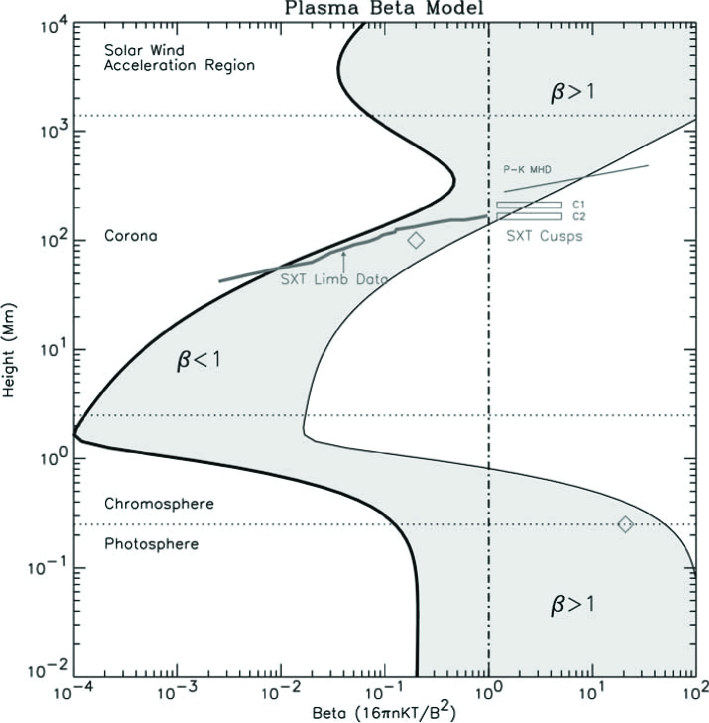
Figure 1: Plasma $\beta$ model over various active regions. The shaded area shows possible plasma $\beta$ corresponds to a sunspot region with 2500 G and a plage region with 150 G. Reproduced with permission from Gary (2001) Copyright 2001, Springer.

Gaining insight into the magnetic fields and plasma in the solar atmosphere is of great importance for studying various solar activities. So far magnetic field measurements in the photosphere are the most reliable. The chromospheric magnetic field measurements confront with much bigger uncertainties and it is difficult to determine the height of the detected magnetic field. The situation in the corona is ever worse since the corona is optical thin and magnetic field measurements have a line of sight integrated character. For constructing the three-dimensional magnetic field configurations in the chromosphere and corona, one may solve a set of equilibrium equations of magnetohydrodynamic (MHD) from given boundary data in the photosphere. This is the so-called magnetic field extrapolation. A popular and powerful extrapolation technique is the nonlinear force-free field (NLFFF) extrapolation which is designed to solve the following equations:

$$\nabla\times\textbf{B} = \alpha(\textbf{r})\textbf{B},$$ (1)

$$\nabla\cdot\textbf{B} = 0,$$ (2)

where B is the magnetic field and $\alpha(\textbf{r})$ is the force-free factor which is constant along a given field line. Equation (1) indicates that the electric current is parallel to the magnetic field, which means a vanishing Lorentz force. Equation (2) is the solenoidal condition of the magnetic field. For recent reviews on the NLFFF extrapolation we refer to Régnier (2013), Guo et al. (2017), and Wiegelmann & Sakurai (2021).

The force-free equation (1) assumes that the plasma $\beta$, defined as the ratio between the plasma pressure and magnetic pressure ($8\pi p/B^{2}$), of the solar atmosphere is low and all non-magnetic forces can be neglected. This is well justified in the most parts of the solar corona. However, it is not the case in the photosphere and lower chromosphere where the plasma pressure is comparable with the magnetic pressure (Gary, 2001). Figure 1 shows that plasma $\beta$ is about unit or larger roughly below 1 Mm above the photosphere. Non-magnetic forces are needed in these regions to balance the Lorentz force. Still assuming a static state, the equilibrium of the lower layers can be described by the magnetohydrostatic (MHS) equations:

$$\frac{1}{4\pi}(\nabla\times\textbf{B})\times\textbf{B}-\nabla p-\rho\nabla\Phi = 0,$$ (3)

$$\nabla\cdot\textbf{B} = 0.$$ (4)

In equation (3), $p$ and $\rho$ are the plasma pressure and density, $\Phi$ is the gravitational potential. To close the above MHS system, we may relate pressure and density with temperature via an equation of state and prescribe an energy-balance equation as follows:

$$p=\rho k_{B}T/m,$$ (5)

$$\nabla\cdot(\textbf{K}\cdot\nabla T)+Q_{rad}+Q_{heat}=0,$$ (6)

with $T$ is the plasma temperature, $k_{B}$ the Boltzmann constant, $m$ the mean molecular weight of the gas, $Q_{rad}$ the source term accounts for heating or cooling owing to radiation, and $Q_{heat}$ the heat source owing to nano-flare, wave dissipation, or other heating mechanisms. $\nabla\cdot(\textbf{K}\cdot\nabla T)$ describes thermal conduction, where K is the thermal conduction coefficient tensor. In particular, the cross-field thermal conduction is much less efficient than the field aligned component. With $Q_{rad}$ and $Q_{heat}$ being prescribed, the above set of partial differential equations (PDEs) (3)–(6) can be solved, in principle, by imposing a set of boundary conditions (B, $p$, and $\rho$) in a finite domain. The technique is called the MHS extrapolation. Note that there are a large number of works on the MHS equilibria for magnetosphere and Tokamak without considering gravity (e.g. Shafranov, 1958; Boozer, 2004; Hesse & Birn, 1993). Here we only concentrate on the three-dimensional MHS equilibria for the solar case, in which gravity cannot be neglected. To our knowledge no review covering this field exists.

Compared with the established NLFFF extrapolation, the MHS extrapolation is much less developed mainly due to the insufficient spatial resolution of the routinely measured vector magnetogram in the past. For example, the spatial resolution of SDO/HMI is about 720 km (Scherrer et al., 2012) which is roughly 1/2 of the thickness of the non-force-free layer. Therefore an extrapolation based on the HMI data does not have sufficient spatial resolution vertically to study the thin non-force-free layer. Furthermore, the pressure scale height on the photosphere is about 150 km, which makes usage of HMI data in resolving this scale questionable. The situation, however, has been changed significantly by new ground-based instruments such as Daniel K. Inouye Solar Telescope (DKIST) which will carry out routine measurements of the magnetic fields in multiple layers with very high spatial resolution (0.03^′′ or 25 km on the solar surface at 500 nm) (Keil et al., 2011).

The aim of this review is to show both analytical and numerical extrapolation techniques which have been developed to solve the MHS equations when the photospheric vector magnetograms are used as the boundary input. The review is organized as follows. The analytical solutions of the MHS equations are discussed in Sect. 2. An overview of the numerical extrapolation techniques are given in Sect. 3. In Sect. 4, we describe the necessary boundary conditions for the MHS equilibrium and give an introduction of a preprocessing algorithm to deal with the inconsistency between the boundary and the MHS assumption. Finally, we summarize and discuss the challenges in the future development of the MHS extrapolation in Sect. 5.

2 Analytical MHS solutions in 3D

The full set of the MHS equations (3)–(6) has two aspects of equilibrium with the force equilibrium achieved by the magnetic fields and plasma, and thermodynamic equilibrium maintained by various energy processes of the plasma. The solution depends on how the two aspects of equilibrium are coupled. An analytical and complete treatment of this problem in 3D is not tractable. Most works has concentrated on seeking solutions of equations (3) and (4) without treating the energy equation self-consistently. The main interest is to find states that are admissible under force equilibrium. In spite of simplifying the equations greatly, they are by no means easy to be solved.

The MHS equilibrium requires some degree of symmetry in the magnetic field, which stems from the balance between Lorentz force and plasma forces (Parker, 1972). The Lorentz force is highly anisotropic while the the plasma forces (pressure gradient and gravitational force) can be derived from isotropic scalar potential. By eliminating pressure term in the x and y components of equation (3) with

$$\frac{\partial^{2}}{\partial x\partial y}(p+B^{2}/8\pi)=\frac{\partial^{2}}{\partial y\partial x}(p+B^{2}/8\pi),$$ (7)

we obtain the symmetry mathematically as follows

$$\frac{\partial}{\partial x}[(\textbf{B}\cdot\nabla)B_{y}]=\frac{\partial}{\partial y}[(\textbf{B}\cdot\nabla)B_{x}].$$ (8)

Equation (8) is also called the compatibility relation which is a necessary but not sufficient condition for an MHS equilibrium. The compatibility relation is trivially satisfied for a system with an ignorable coordinate. For example, consider a two-dimensional plasma with $\frac{\partial}{\partial x}=0$, the left hand side of equation (8) then vanishes. The right hand side of equation (8) also vanishes because $(\textbf{B}\cdot\nabla)B_{x}=0$ which represents a null tension force in x-direction. The compatibility relation is also satisfied under rotational and helical symmetries. Substantial efforts have been made to treat the MHS equations by ignoring a coordinate (e.g. Dungey, 1953; Low, 1975; Hundhausen et al., 1981; Uchida & Low, 1981; Amari & Aly, 1989). The symmetry introduced by the ignored coordinate render the MHS problem tractable.

However, the real solar structures observed are highly inhomogeneous and seldom show a high degree of geometric symmetry. On the other hand, the need of symmetry in the magnetic field does not necessarily mean an ignorable coordinate. Works by giving up the assumption of an ignorable coordinate have been conducted and some families of particular three-dimensional MHS solutions have been found. Low (1982) found a family of three-dimensional MHS equilibria by assuming that the magnetic field lines lie in parallel vertical planes. Except for this assumption, structural variation of the system is allowed in all three dimensions. The constraint of the laminar magnetic field structure was relaxed in Low by demanding the magnetic tension force being vertical (Low, 1984):

$$(\textbf{B}\cdot\nabla)B_{x}=0,$$ (9)

$$(\textbf{B}\cdot\nabla)B_{y}=0.$$ (10)

With equations (9) and (10), the compatibility condition is satisfied trivially. Hu et al. (1983) built a slightly non-axisymmetric equilibrium with a perturbation theory. In their approach, an perturbation expansion was carried out to the originally axisymmetric magnetic flux tube.

Although these solutions are three-dimensional, they are not consistent with the measured line-of-sight (LOS) magnetogram due to some regularity imposed through the compatibility condition. It means that the previous solutions cannot be used to model the real Sun. This situation has not been changed until Low (1985) (hereinafter L85) found a new class of three-dimensional MHS equilibria. The new equilibria which assume a horizontal electric current everywhere are capable of cooperating with arbitrary distribution of LOS magnetic field as the boundary condition. This characteristic makes the new solution applicable to model the real solar atmosphere, while previously only potential field (Schmidt, 1964) and linear force-free field (Chiu & Hilton, 1977) had reached the level of sophistication. After that, a number of works have been stimulated based on the assumption made in L85. The following reviews these works.

2.1 Analytical solution with untwisted magnetic field

L85 derives a set of analytical and fully three-dimensional solutions of the MHS equations which are applicable to extrapolate the magnetic field and plasma from the observed magnetogram. The key assumption is to take the electric current to be everywhere perpendicular to the gravitational force. It follows that the transverse components of equation (3) resolve into

$$\frac{\partial B_{z}}{\partial x}\frac{\partial}{\partial y}\left(\frac{\partial\phi}{\partial z}\right)-\frac{\partial B_{z}}{\partial y}\frac{\partial}{\partial x}\left(\frac{\partial\phi}{\partial z}\right)=0,$$ (11)

where $\phi$ is defined as

$$\textbf{B}=\left\{\frac{\partial\phi}{\partial x},\frac{\partial\phi}{\partial y},B_{z}\right\}.$$ (12)

Note that equation (11) is equivalent of the compatibility relation equation (8). The general solution of equation (11) is

$$B_{z}=\Psi\left(\frac{\partial\phi}{\partial z},z\right),$$ (13)

where $\Psi$ is an arbitrary function of its arguments. Substitute equation (13) into magnetic divergence free equation (4), then we obtain

$$\frac{\partial^{2}\phi}{\partial x^{2}}+\frac{\partial^{2}\phi}{\partial y^{2}}+\frac{\partial}{\partial z}\Psi\left(\frac{\partial\phi}{\partial z},z\right)=0.$$ (14)

For each prescription of $\Psi$, equation (14) can be solved with the classical Neumann boundary condition of $\phi$

$$S_{0}:\frac{\partial\phi}{\partial z}=\Psi^{*}(B_{z},0),$$ (15)

where $S_{0}$ is the bottom boundary and $\Psi^{*}$ is the inverse of $\Psi$ to express $\frac{\partial\phi}{\partial z}$ as a function of $B_{z}$ and $z$. Once $\phi$ is known, equation (13) determines $Bz$, and equation (12) yields B. For each B constructed, we can derive $p$ and $\rho$ directly through integrating the MHS equation (3) at different directions.

The basic principle of the above solution is to reduce the MHS equations (3) and (4) to a single, scalar PDE (14). The reduction is, of course, allowed by assuming a special type of electric current which is everywhere perpendicular to gravity and distributed smoothly in space. It is worth noting that the energy equation is omitted and the equation of state is not fixed a priori in this method. The governing equations are thus closed by prescribing the function $\Psi$ of its arguments $\frac{\partial\phi}{\partial z}$ and $z$.

L85 studied a particular solution with

$$\Psi=\gamma\frac{\partial\phi}{\partial z}$$ (16)

where $\gamma$ is a constant. They found magnetic field of the solution ($\gamma\neq 1$) can be obtained from the corresponding potential field ($\gamma=1$) by a uniform vertical expansion or contraction. Thus, the particular solution has a magnetic topology identical to that of the potential field. The same solution has also been expressed in spherical geometry with a point mass by Bogdan & Low (1986) (hereinafter BL86).

A more general formulation of the MHS equations was presented in Low (1991) (hereinafter L91) by using electric current represented in terms of a pair of Euler potential $\mu$ and $\nu$:

$$\nabla\times\textbf{B}=\nabla\mu\times\nabla\nu.$$ (17)

L91 assumed $\nu$ coincides with $\Phi$ (with $\Phi$ the gravitational potential) which sets the electric current to be perpendicular to gravity. He found $\mu$ is a function of only two independent variables $\textbf{B}\cdot\nabla\Phi$ and $\Phi$:

$$\mu=F(\textbf{B}\cdot\nabla\Phi,\Phi).$$ (18)

It follows

$$\nabla\times\textbf{B}=\nabla F(\textbf{B}\cdot\nabla\Phi,\Phi)\times\nabla\Phi.$$ (19)

The formulation (19) can be easily applied to any potential $\Phi$ which represents combination of any gravitational force and inertial force such as centrifugal force. Another advantage is to allow the magnetic field to have net twist, which will be discussed in the following subsection.

The MHS equations have also been reduced by using Clebsch representation, which have been presented by Osherovich (1985a, b). To obtain an analytical solution, Osherovich (1985a) also used a special type of electric flow which is perpendicular to the gravity.

2.2 Analytical solution with twisted magnetic field

The main disadvantage of the case studied above is that the magnetic field does not have a net twist. The only exception exists when the magnetic field lies in the surfaces of constant $\Phi$, which is way far from reality.

To circumvent the deficiency, L91 added a field-aligned electric current component. Then the two current systems can be expressed, in Cartesian coordinates with $\Phi=gz$, as

$$\nabla\times\textbf{B}=\alpha\textbf{B}+\nabla F(B_{z},z)\times\hat{\textbf{z}},$$ (20)

where $\alpha$ is a constant in space. Note that equations (19) and (20) share the same mathematic form of the current perpendicular to the gravity. With a prescribed $F$, the governing equations (20) and (4) for four unknowns are in general complete as a system.

For the case that function $F$ is linear in $B_{z}$, e.g.,

$$F=f(z)B_{z}$$ (21)

as suggested by L91, equation (20) can be reduced to a linear form

$$\nabla\times\textbf{B}=\alpha\textbf{B}+f(z)\nabla B_{z}\times\hat{\textbf{z}}.$$ (22)

Fourier transforming of equation (22) with respect to $(x,y)\mapsto(h,k)$ (so $\textbf{B}(x,y,z)\mapsto\tilde{\textbf{B}}(h,k,z)$) leads to a single, second order, and ordinary differential equation of $\tilde{B_{z}}$ as

$$\frac{d^{2}\tilde{B_{z}}}{dz^{2}}+\left\{\alpha^{2}+(h^{2}+k^{2})\left[f(z)-1\right]\right\}\tilde{B_{z}}=0.$$ (23)

Then $\tilde{B_{x}}$ and $\tilde{B_{y}}$ can be expressed in terms of $\tilde{B_{z}}$ as

$$\tilde{B_{x}} = \frac{i}{h^{2}+k^{2}}\left(h\frac{d\tilde{B_{z}}}{dz}+k\alpha\tilde{B_{z}}\right),$$ (24)

$$\tilde{B_{y}} = \frac{i}{h^{2}+k^{2}}\left(k\frac{d\tilde{B_{z}}}{dz}-h\alpha\tilde{B_{z}}\right).$$ (25)

An inverse Fourier transformation is thus applied to recover B. It follows the distribution of plasma pressure and density:

$$p = p_{0}(z)-\frac{1}{8\pi}f(z)B_{z}^{2},$$ (26)

$$\rho = -\frac{1}{g}\frac{dp_{0}}{dz}+\frac{1}{4\pi g}\left[\frac{1}{2}\frac{df}{dz}B_{z}^{2}+f\textbf{B}\cdot\nabla B_{z}\right].$$ (27)

The first terms of equations (26) and (27) describe the stratified atmosphere and the second terms are the modifications by the non-force-free magnetic field.

Low (hereinafter L92) assumed that $f(z)$ has the following structure

$$f(z)=ae^{-\kappa z},$$ (28)

where $a$ and $\kappa$ control the intensity and characteristic length of Lorentz force (Low, 1992). Then the general solution of equation (23) takes the form:

$$\tilde{B_{z}}=M_{h,k}J_{s}[qe^{(-\kappa z)}]+N_{h,k}J_{-s}[qe^{(-\kappa z)}],$$ (29)

where $\tilde{B_{z}}$ represents the Fourier transformation associated with component $e^{i(hx+ky)}$, $J_{s}$ and $J_{-s}$ are the Bessel functions, $M_{h,k}$ and $N_{h,k}$ are integration constants, $q^{2}=4a(h^{2}+k^{2})/\kappa^{2}$, and $s^{2}=4(h^{2}+k^{2}-\alpha^{2})/\kappa^{2}$. In solar applications, $J_{-s}$ term is rejected by setting $N=0$ since the magnetic field vanishes at infinity high above photosphere. Then $M$ can be determined using the observed photospheric magnetogram. L92 applied the MHS solution to an artificial active region magnetogram and showed a lot of interesting features, such as density enhancement along the neutral line at the lower atmosphere, twisted magnetic flux rope, etc. The high density plasma above the neutral line supported by the helical magnetic flux rope is interpreted as chromospheric filament.

With alternative structures of $f(z)$ many families of the MHS solutions have been found. Neukirch (1995) reduced equation (22) to a Schrödinger type equation which has been intensively studied in quantum mechanisms. With the new tool he derived three families of the MHS solutions corresponding to three choices of $\xi(r)$ for a spherical self-gravitating body. Here

$$r^{2}\xi(r)=1-\frac{1}{\eta(r)},$$ (30)

where $\eta(r)$ the counterpart of $f(z)$ in Cartesian coordinates. Petrie & Neukirch (2000) also studied the MHS solutions for three different choices of $f(z)$ by the Green’s function method. Neukirch & Wiegelmann (2019) presented a solution with

$$f(z)=a\left[1-b\,\textmd{tanh}\left(\frac{z-z_{0}}{\triangle z}\right)\right],$$ (31)

where a and b control the magnitude of f, $\triangle z$ controls the width of a transition from non-force-free to force-free field. The height and width of the transition being specified by the model parameters makes the new solution more flexible, which is also important to keep the plasma pressure and density positive.

For the case that function $F$ is nonlinear in $B_{z}$, i.e.,

$$F=\frac{B_{z}}{4\pi}+f(z)B_{z}^{n},$$ (32)

Neukirch (1997) presented a family of solutions which have an arcade-like magnetic field topology.

An alternative mathematical formulation for calculating the MHS equilibrium was introduced by Neukirch & Rastätter (1999) with the magnetic field represented in terms of poloidal and toroidal components

$$\textbf{B}=\nabla\times\nabla\times(P\hat{\textbf{z}})+\nabla\times(T\hat{\textbf{z}}),$$ (33)

where P and T are two scalar functions. This has an advantage that equation (20) can be reduced to only one scalar PDE with the following form

$$\nabla^{2}P+\alpha^{2}P+F(z,B_{z}) = 0,$$ (34)

$$T-\alpha P = 0.$$ (35)

Thus P gains full knowledge of the complete magnetic field, which is very similar to the well-known case of linear force-free magnetic field Nakagawa & Raadu (1972). Previously, however, the three components of the magnetic field have to be computed separately. The Neukirch & Rastätter (1999) model has been calculated efficiently with a multi-grid approach implemented by MacTaggart et al. (2013).

Solutions of the MHS equations with more general external potentials, such as centrifugal force in a rotating system, have been described in both spherical coordinate (Low, 1991; Neukirch, 2009; Al-Salti & Neukirch, 2010) and cylindrical coordinate (Al-Salti et al., 2010; Wilson & Neukirch, 2018).

It is worth noting that, by taking divergence of equation (20), the two current systems are conserved separately (Low, 1993). An interesting inference from the uncoupled currents is that there exists magnetic flux-current surface where the magnetic flux surface and the current surface overlap (Choe & Minhwan, 2013). Low (1993) showed that all MHS equilibria of symmetric system have uncoupled electric currents with two independent coordinates. He also pointed out that the coupled currents equilibria which require three independent coordinates are a distinct class of the MHS solutions from the uncoupled one.

2.3 Determination of parameters $\alpha$, $a$, and $\kappa$

The L91 solution has three unknowns $\alpha$, a, and $\kappa$ (see equations (20) and (28)). $\kappa$ is the reciprocal of the scale height above which the solution will become approximately force-free due to the low plasma $\beta$. The scale height often refers to the typical height of chromosphere where a significant interaction between the magnetic field and plasma takes place, leading to $1/\kappa=2$ Mm (Aulanier et al., 1998; Wiegelmann et al., 2015, 2017). The remaining parameters $\alpha$ and $a$ characterize field-aligned current system and horizontal current system, respectively. They may be varied to best fit observations. Figure 2 illustrates how the magnetic structure changes with various choices of $\alpha$ and $a$. Note that $\alpha=a=0$ recovers potential field, while only $a=0$ recovers linear force-free field. If only $\alpha=0$ we recover L85 and BL86 model.

In the presence of vector magnetogram of an active region, $\alpha$ can be constrained by horizontal photospheric magnetic field vector. Wiegelmann et al. (2017) used SUNRISE/IMaX vector magnetograms (Solanki et al., 2017) to compute $\alpha$ following an approach developed by Hagino & Sakurai (2004) for linear force-free fields:

$$\alpha=\frac{\sum\left(\frac{\partial B_{y}}{\partial x}-\frac{\partial B_{x}}{\partial y}\right)sign(B_{z})}{\sum|B_{z}|},$$ (36)

where the summation is taken over pixels of the magnetogram. In the absence of the vector magnetogram or the inaccurate measurements of the vector magnetic field due to poor signal-to-noise-ratio such as in the quiet regions, $\alpha$ is a free parameter to some extent. An additional restriction on $\alpha$, as discussed by Aulanier & Demoulin (1998) and Aulanier et al. (1998), is that $\alpha$ has a maximum value of $\alpha_{max}=2\pi/L$, where $L$ is the horizontal length of the computational box. L91 and L92 also showed that all modes with wavenumbers $h$ and $k$ in the domain $s^{2}=4(h^{2}+k^{2}-\alpha^{2})/\kappa^{2}<0$ (see general solution (29)) oscillate with a nonvanishing amplitude as $z\rightarrow\infty$, and thus these modes should be rejected. To allow the solution to be applied to an arbitrary magnetogram, all wavenumbers should be included. This is ensured by $\alpha<2\pi/L$ since a periodic computational box with horizontal length $L$ has a minimum wavenumber $2\pi/L$. The property encountered here in the linear MHS solution has also been encountered previously in the study of linear force-free field. It is not accidental that the two models share the property because the linear MHS field becomes the linear force-free field in the limit of $\kappa z\gg 1$.

To constrain $a$ is a more challenging task. The dimensionless parameter $a$ controls the horizontal current which includes both magnetic field aligned and perpendicular components. The latter component gives rise to Lorentz force. Recall that the Lorentz force can be calculated by integrating Maxwell stress tenser $T$ over the entire surface over the computational volume (Molodensky, 1969, 1974). In the solar applications, a normalized parameter $\epsilon$ has been suggested by Wiegelmann et al. (2006) to check force-freeness of the magnetogram. $\epsilon$ is defined as

$$\epsilon=\frac{|\sum B_{x}B_{z}|+|\sum B_{y}B_{z}|+|\sum(B_{x}^{2}+B_{y}^{2}-B_{z}^{2})|}{\sum(B_{x}^{2}+B_{y}^{2}+B_{z}^{2})},$$ (37)

where the summation is taken over pixels of the magnetogram, each term in numerator represents Lorentz force in each direction. Thus both $a$ and $\epsilon$ relate to the Lorentz force. Wiegelmann et al. (2017) suggested a linear relationship between them, empirically, as

$$a=2\epsilon.$$ (38)

By using equation (38), $a$ can be specified in the presence of vector magnetogram. In the absence of vetor magnetogram, Aulanier et al. (1998) pointed out that $a$ has a maximum value $a_{max}$ to make the solution physical. To see this, the MHS solution (29) is reduced by rejecting $J_{-s}$ term in solar applications:

$$\tilde{B_{z}}=M_{h,k}J_{s}[qe^{(-\kappa z)}].$$ (39)

$J_{s}$ changes its sign as its argument increases, which implies an oscillation behavior of the magnetic field amplitude. Aulanier et al. (1998) took this behavior unphysical. They further found a reaches its maximum when $z=0$ and, under the extreme case, determined $a_{max}=1$.

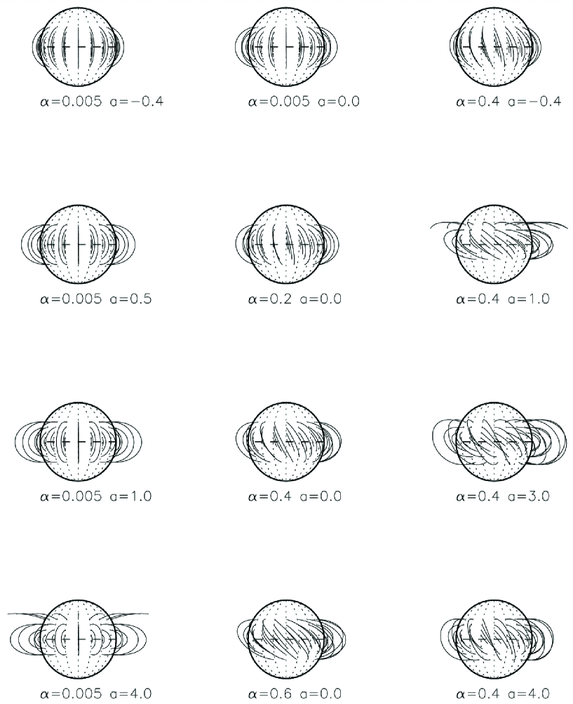
Figure 2: Influence of $\alpha$ and $a$ on the magnetic structure of the global corona. $\alpha$ and $a$ are normalized by $1/r_{0}$ and $r_{0}$, respectively, where $r_{0}$ is the radius of the Sun. It is worth to stress that definition of the parameter $a$ (see equation (1) in Zhao et al. (2000)) used in this figure is slightly different than dimensionless $a$ defined in equation (28). However, they both characterize the horizontal electric current system. The magnetic field line expands as $a$ increases, and it becomes twisted as $\alpha$ increases. Reproduced with permission from Zhao et al. (2000) Copyright 2000, AAS.

2.4 Boundary conditions

As input the analytical MHS models require normal magnetic field $B_{n}$ measured at the photosphere. In the presence of high-quality vector magnetogram, $\alpha$, as a constant, can be constrained meaningfully. For a more general MHS case with

$$\textbf{B}\cdot\nabla\alpha=0$$ (40)

rather than $\alpha$ being a constant everywhere, Low (2005) found that the closed contours of constant $\alpha$ at the boundary must come in pairs of equal total enclosed boundary flux. The topological property relating $\alpha$ and $B_{n}$ through “hyperbolic” equation (40) was first pointed out by Aly (1989) for force-free fields and is still applicable for the MHS case with two-current system. Then Low (2005) derived a complete set of boundary conditions which contain the arbitrarily prescribed $B_{n}$ and a restricted $\alpha$ distribution. $\alpha$ needs to satisfy

$$\alpha(x,y,0)=G(g(x,y,0)),$$ (41)

where $G$ is an even function and $g(x,y,0)$ takes the values of equal and opposite total boundary flux enclosed by each of $\alpha$ contour.

2.5 Applications of the analytical MHS solutions to measured magnetograms

Despite the limitations of the transverse current assumption, the analytical solutions have been used to study solar MHS equilibria in various situations. Since only the linear solution has been applied so far, the analytical MHS solution is often named the linear MHS solution in practice.

Some studies have focused on the lower atmosphere. Aulanier et al. (1998) modeled the magnetic field configuration of an H$\alpha$ flare by using L91 solution. They found the presence of dense plasma in regions of dipped field lines, which is in agreement with dark elongated features in H$\alpha$. The model also revealed that the flare kernels are located at separatrices correlated to “bald patches” (BPs) where field lines are tangential to the photosphere. The extrapolated BPs by the analytical MHS solutions have also been found associated with arch filament system and surge in chromosphere and transition region brightening (Fletcher et al., 2001; Mandrini et al., 2002). Comparisons between the analytical MHS solution and linear force-free solution have showed that the plasma effect helps to improve the magnetic configuration with a better correspondence with observation (Aulanier et al., 1999; Dudík et al., 2008). Wiegelmann et al. (2015) and Wiegelmann et al. (2017), using L91 solution with magnetograms measured by the magnetograph IMaX (Martínez Pillet et al., 2011) on board SUNRISE (Solanki et al., 2010, 2017), modeled the magnetic field as well as plasma of a quiet region and an active region, respectively. Thanks to the high resolution of the magnetogram ($\sim 100$ km), the modeling resolves the thin non-force-free layer (typically less than 2000 km) with tens of grid points. Using the extrapolation data by Wiegelmann et al. (2017), Jafarzadeh et al. (2017) found the majority of slender Ca II H fibrils saw in SUNRISE/SuFI instrument overlap magnetic field lines at a height of around 700-1000 km. These field lines show a canopy-like dome over quiet areas.

Other studies have concentrated on global modeling of the solar corona (see review by Mackay & Yeates, 2012). The most widely used method to model the corona globally is the potential field source surface (PFSS) model which assumes a free current between the photosphere and the source surface. However, the current-free assumption is oversimplified because we have routinely observed large scale plasma structures, such as helmet streamers and coronal loop arcades, in multiple wavelengths which show appreciable interaction between magnetic field and plasma. Bagenal & Gibson (1991), Gibson & Bagenal (1995) and Gibson et al. (1996) showed that the BL86 solution may account for the large-scale non-sphericity of the corona. The authors also found it necessary to include current sheets at equator and around the helmet streamer in the model to match white light observation of the corona during solar minimum. Zhao & Hoeksema (1993, 1994, 1995) developed a global model to map the observed photospheric magnetic field into the corona and interplanetary space. A spherical “cusp surface” was defined at which all helmet streamer cusp points located identically. Below the cusp surface (or inner corona), the authors built an MHS atmosphere with BL86 solution. Then they extended the BL86 solution to larger radii with current sheets model developed by Schatten (1971). Their model better reproduces corona streamers and helmet structures as well as observed interplanetary magnetic field near the Earth’s orbit. The BL86 solution have also been applied to recover the coronal fine structures observed during total solar eclipse (Ambrož et al., 2009; Yeates et al., 2018). The more general solution based on BL86 by adding field-aligned current component (Neukirch, 1995) has also been used for corona modeling globally (Zhao et al., 2000; Rudenko, 2001; Ruan et al., 2008). Zhao et al. (2000) found the magnetic arcade computed with $\alpha=0$ agrees best with the well-developed polar crown soft X-ray arcade, which suggests that the well-developed soft X-ray arcade has no field-aligned currents. Ruan et al. (2008), using the Neukirch (1995) model, found the large structure of the magnetic field configuration is described reasonably well.

3 Numerical approaches for the MHS extrapolation

Applying a linear MHS solution of equations (3) and (4) to model the sun has its limitation. The limitation has to do with the constant $\alpha$ and $a$ over the computational region, which makes the model fail to recover magnetic configurations with strong electric current concentration in part of the domain. A similar restriction occurs in the linear force-free modeling with globally constant $\alpha$. The linear MHS model also encounters a problem of negative plasma pressure in applications to solar quiet region. To circumvent these deficiencies, some numerical approaches have been developed recently to solve the MHS equation.

In the following, we briefly describe three different numerical approaches for computing solar MHS equilibria from photospheric vector magnetograms. The optimization method for MHS modeling was proposed by Wiegelmann & Neukirch (2006) and further developed by Zhu & Wiegelmann (2018, 2019). The MHD relaxation method for MHS modeling was developed by Zhu et al. (2013) and Miyoshi et al. (2020). The Grad-Rubin method for MHS modeling was proposed by Gilchrist & Wheatland (2013) and Gilchrist et al. (2016). Both optimization method and MHD relaxation method use three components of vector magnetogram as magnetic boundary conditions, while the Grad-Rubin method uses vertical magnetic field and vertical electric current density as the boundary condition from observation. Every method requires the potential field as their very initial guess of the magnetic field.

3.1 Optimization method

We rewrite equation (3) with a constant gravitational acceleration as follows:

$$(\nabla\times\textbf{B})\times\textbf{B}-\nabla p-\rho\hat{\textbf{z}}=0.$$ (42)

To display most clearly the mathematical structure of the equation, we have set relevant physical constants to unity. The optimization method for the MHS modeling is to find solution of the MHS equations (42) and (4) by minimizing functional

$$L(\textbf{B},p,\rho)=\int_{V}B^{2}(\Omega_{a}^{2}+\Omega_{b}^{2})dV,$$ (43)

where

$$\Omega_{a} = B^{-2}[(\nabla\times\textbf{B})\times\textbf{B}-\nabla p-\rho\hat{\textbf{z}}],$$ (44)

$$\Omega_{b} = B^{-2}[(\nabla\cdot\textbf{B})\textbf{B}].$$ (45)

It is obvious that $L\geq 0$. If the minimization process reaches $L=0$ then the MHS equations are fulfilled. Taking the functional derivative of the functional (43) with respect to the iteration parameter $t$ we have:

$$\frac{1}{2}\frac{dL}{dt}=-\int_{V}\left(\frac{\partial\textbf{B}}{\partial t}\cdot\textbf{F}-\frac{\partial p}{\partial t}\nabla\cdot\textbf{$\Omega_{a}$}+\frac{\partial\rho}{\partial t}\textbf{$\Omega_{a}$}\cdot\hat{\textbf{z}}\right)dV-\oint_{S}\left(\frac{\partial\textbf{B}}{\partial t}\cdot\textbf{G}+\frac{\partial p}{\partial t}\textbf{$\Omega_{a}$}\right)\cdot\textbf{dS},$$ (46)

where

F $$= \nabla\times(\textbf{$\Omega_{a}$}\times\textbf{B})-\textbf{$\Omega_{a}$}\times(\nabla\times\textbf{B})+\nabla(\textbf{$\Omega_{b}$}\cdot\textbf{B})-\textbf{$\Omega_{b}$}(\nabla\cdot\textbf{B})+(\Omega_{a}^{2}+\Omega_{b}^{2})\textbf{B},$$ (47)

G $$= \hat{\textbf{n}}\times(\textbf{$\Omega_{a}$}\times\textbf{B})-\hat{\textbf{n}}(\textbf{$\Omega_{b}$}\cdot\textbf{B}).$$ (48)

Given a fixed boundary condition the surface term vanishes. Then the gradient descent method is used to iterate B, $p$, and $\rho$ by

$$\frac{\partial\textbf{B}}{\partial t} = \mu_{1}\textbf{F},$$ (49)

$$\frac{\partial p}{\partial t} = -\mu_{2}\nabla\cdot\textbf{$\Omega_{a}$},$$ (50)

$$\frac{\partial\rho}{\partial t} = \mu_{3}\textbf{$\Omega_{a}$}\cdot\hat{\textbf{z}}.$$ (51)

With positive constants $\mu_{1}$, $\mu_{2}$, and $\mu_{3}$, $L$ decreases monotonically.

The optimization method was first proposed by Wheatland et al. (2000) to calculate the NLFFF. Wiegelmann & Neukirch (2006) extended the method by introducing plasma pressure in Cartesian geometry. They tested the code with an analytical MHS equilibrium (without gravity) similar to the force-free Low & Lou (1990) solution and found the reconstructed solution agrees well with the reference model. They also found the computing time of the MHS optimization is about 1000 times larger than the corresponding force-free optimization. The reason for the slow convergence is because plasma pressure in the reference model has a huge difference with 25 orders of magnitude.

Wiegelmann et al. (2007) further extended the method by including gravitational forces in spherical geometry to calculate the global solar corona. The test of the code with a linear MHS solution by Neukirch (1995) showed the method works well and converges to the reference solution. However, the poles of the spherical geometry requires a sufficiently small time-step, which further slows down the optimization process. They suggested to use the Yin-Yang grid (Kageyama & Sato, 2004) to address the problem.

Minimizing functional (43) subjects to constraints on plasma pressure and mass density which must be positive. However, it is not guaranteed by the previous methods. Zhu & Wiegelmann (2018) eliminated the constraints by using the variable transformation

$$p = Q^{2},$$ (52)

$$\rho = R^{2}.$$ (53)

Then the constrained problem is simplified to an unconstrained one

$$minimize\quad L(\textbf{B},Q,R)=\int_{V}B^{2}(\Omega_{a}^{2}+\Omega_{b}^{2})dV,$$ (54)

where

$$\Omega_{a} = \frac{(\nabla\times\textbf{B})\times\textbf{B}-\nabla Q^{2}-R^{2}\hat{\textbf{z}}}{B^{2}+Q^{2}},$$ (55)

$$\Omega_{b} = \frac{(\nabla\cdot\textbf{B})\textbf{B}}{B^{2}+Q^{2}}.$$ (56)

Note that the denominators $(B^{2}+Q^{2})$ in equations (55) and (56) are different than denominators $B^{2}$ in the previous method. Without plasma pressure in the denominator, $L$ will be dominated by regions with extremely weak magnetic field (Zhu & Wiegelmann, 2019). The minimization problem (54) then leads to

$$\frac{\partial\textbf{B}}{\partial t} = \mu_{1}\textbf{F},$$ (57)

$$\frac{\partial Q}{\partial t} = \mu_{2}Q\left[\lambda(\Omega_{a}^{2}+\Omega_{b}^{2})-\nabla\cdot(\lambda\textbf{$\Omega_{a}$})\right],$$ (58)

$$\frac{\partial R}{\partial t} = \mu_{3}R\lambda\textbf{$\Omega_{a}$}\cdot\hat{\textbf{z}},$$ (59)

where

F $$= \nabla\times(\lambda\textbf{$\Omega_{a}$}\times\textbf{B})-\lambda\textbf{$\Omega_{a}$}\times(\nabla\times\textbf{B})+\nabla(\lambda\textbf{$\Omega_{b}$}\cdot\textbf{B})-\lambda\textbf{$\Omega_{b}$}(\nabla\cdot\textbf{B})+(1-2\lambda)(\Omega_{a}^{2}+\Omega_{b}^{2})\textbf{B},$$ (60)

$$\lambda = \frac{B^{2}}{B^{2}+Q^{2}}.$$ (61)

The computational implementation involves the following steps.

1. Calculate NLFFF (Wiegelmann, 2004) using vector magnetogram preprocessed with force-free criteria (Wiegelmann et al., 2006).

2. Determine plasma pressure in the photosphere with formula $p=p_{quiet}-B_{z}^{2}/2$ with $p_{quiet}$ the plasma pressure in the quiet region. Distribute plasma along the magnetic field line by assuming gravitational stratification with a one-dimensional temperature profile.

3. Iterate for $\textbf{B},Q$ and $R$ by equations (57)-(59). This step is repeated until $L$ reaches its minimum.

Note that the bottom boundary condition of the plasma pressure ($p+B_{z}^{2}/2=p_{quiet}$) is simply the force balance condition of a hypothetically vertical magnetic flux tube. The rationality of the boundary setting can also be explained that the plasma pressure is related only with the vertical magnetic field in the linear MHS case. We take it as the lowest-order approximation in the nonlinear case.

The optimization code in the implementation of Zhu & Wiegelmann (2018) has recently been extended toward injecting the vector magnetogram slowly. By slow injection the initial magnetic field at the bottom boundary adjusted continuously by the gradient descent method over the total iterations of the calculation. The idea is to deal with measurement errors in photospheric vector magnetograms in particular in the transverse field. The slow injection approach is found to be capable of improving reconstructed magnetic field in both NLFFF and MHS calculations (Wiegelmann et al., 2012; Zhu & Wiegelmann, 2019).

Zhu & Wiegelmann (2018, 2019) have tested the performance of the code applied to an analytical MHS solution (L91) and RMHD numerical simulation (Cheung et al., 2019). It has been investigated how the unknown lateral and top boundaries, unknown bottom plasma boundary, initial conditions, and noise of magnetogram influence the solution. The code has also been applied to model the solar atmosphere with the high-resolution SUNRISE/IMaX vector magnetograms as well as moderate-resolution SDO/HMI vector magnetograms (Zhu et al., 2020; Hou et al., 2021; Jafarzadeh et al., 2021).

3.2 MHD relaxation method

The MHD relaxation method uses time-dependent MHD equations to compute static equilibria. It has been widely applied to construct NLFFFs (Mikic et al., 1988; Roumeliotis, 1996; McClymont et al., 1997; Valori et al., 2005; Jiang & Feng, 2012; Guo et al., 2016). Recently, the method has been extended to construct MHS equilibria. The main idea is to solve either full or simplified MHD equations with plasma forces (e.g., pressure gradient and gravitational force) by using a friction term to relax the system into a quasi-static equilibrium.

Zhu et al. (2013) developed an MHD relaxation method by solving the full compressive MHD equations which are given as follows:

$$\frac{\partial\rho}{\partial t} = -\nabla\cdot(\rho\textbf{v}),$$ (62)

$$\rho\left(\frac{\partial\textbf{v}}{\partial t}+\textbf{v}\cdot\nabla\textbf{v}\right) = \frac{1}{4\pi}(\nabla\times\textbf{B})\times\textbf{B}-\nabla p+\rho\textbf{g}-\mu\rho\textbf{v},$$ (63)

$$\frac{\partial e}{\partial t} = -p\nabla\cdot\textbf{v}-\mu\rho v^{2},$$ (64)

$$\frac{\partial{\textbf{B}}}{\partial t} = \nabla\times(\textbf{v}\times\textbf{B}),$$ (65)

where $-\mu\rho\textbf{v}$ is the friction term with coefficient $\mu$ represents the reciprocal of timescale of velocity damping. The initial condition is a potential magnetic field determined by the vertical component of the magnetogram, together with a gravity-stratified atmosphere including changes from the photosphere to the corona. Then the measured transverse magnetic fields are injected slowly at the bottom boundary (Roumeliotis, 1996), while other physical quantities are fixed to their initial values. Deviation from equilibrium leads to plasma movements. Then the velocity is dissipated due to friction and finally a high-$\beta$ and non-force-free equilibrium is established in the lower atmosphere.

Zhu et al. (2013) also performed a test of the code on a numerical simulation of an active region emergence. Quantitative comparisons show that the method works well in extrapolating the non-force-free magnetic field. However, the distribution of plasma temperature is not well recovered. The code has also been applied to study solar activities in the lower atmosphere such as H$\alpha$ fibrils (Zhu et al., 2016), small-scale filament (Wang et al., 2016), ultraviolet burst (Zhao et al., 2017; Tian et al., 2018; Chen et al., 2019), and blowout jet (Zhu et al., 2017). Other applications focus on large-scale structures of the magnetic fields in the corona also show the robustness of the method (Song et al., 2018; Miao et al., 2018; Joshi et al., 2019; Song et al., 2020; Fu et al., 2020).

Recently, Miyoshi et al. (2020) developed an MHD relaxation method to reconstruct the non-force-free equilibrium by solving a set of simplified MHD equations given as follows:

$$\frac{\partial\textbf{v}}{\partial t} = (\nabla\times\textbf{B})\times\textbf{B}-\nabla\tilde{p}-\frac{\tilde{p}}{H_{0}(z)}\hat{\textbf{z}}-\mu\textbf{v},$$ (66)

$$\frac{\partial\textbf{B}}{\partial t} = \nabla\times(\textbf{v}\times\textbf{B}-\eta\nabla\times\textbf{B}),$$ (67)

$$\frac{\partial\tilde{p}}{\partial t} = -a^{2}\nabla\cdot\textbf{v},$$ (68)

where $-\mu\nu$ is the friction term,

$$\tilde{p}=p-p_{0}(z)$$ (69)

is the pressure deviation from hydrostatic $p_{0}(z)$ of the background, and $H_{0}(z)$ is the pressure scale height defined by

$$H_{0}(z)\equiv\frac{T_{0}(z)}{g}.$$ (70)

They assumed that both atmosphere and background atmosphere share the same temperature profile $T_{0}(z)$ which depends on $z$ only. Hence, the density deviation is given by

$$\tilde{\rho}=\frac{\tilde{p}}{T_{0}(z)},$$ (71)

which removes $\tilde{\rho}$ in equation (66). Note that both $\tilde{p}$ and $\tilde{\rho}$ can be negative. The initial condition is the same with that of Zhu et al. (2013). Pressure deviation at the boundary during the relaxation process is extrapolated from the values in the computational area. The code has been tested in two-dimensional problem, but it is implemented in three dimensions.

3.3 Grad-Rubin method

The Grad-Rubin method was first proposed for fusion plasma by Grad & Rubin (1958). Applications to NLFFFs can be found in Sakurai (1981), Amari et al. (1999), and Wheatland (2007). The idea of the Grad-Rubin method is to replace the nonlinear equations to be solved by a system of linear equations, and then solve the linear equations iteratively until a fixed point is reached.

The first MHS implementation of the Grad-Rubin method was developed by Gilchrist et al. with $\textbf{g}=0$ (Gilchrist & Wheatland, 2013). Gilchrist et al. extended the method to solve the MHS equations with $\textbf{g}\neq 0$ (Gilchrist et al., 2016). In their approach, $p$ and $\rho$ are not independent since scale height $H(\textbf{r})$ is prescribed everywhere. To avoid instabilities due to spurious electric currents in weak-field regions, $p$ and $\rho$ are split into background ($p_{0}$ and $\rho_{0}$) and deviation ($\tilde{p}$ and $\tilde{\rho}$) components and each is computed separately. Then the MHS force-balance equation is reformulated in terms of $\tilde{p}$ as

$$\textbf{J}\times\textbf{B}-\nabla\tilde{p}-\left[\frac{p_{0}(z)+\tilde{p}}{H(\textbf{r})}-\frac{p_{0}(z)}{H_{0}(z)}\right]\hat{\textbf{z}}=0.$$ (72)

The boundary condition on J, B, and $\tilde{p}$ are specified as follows:

$$\textbf{B}\cdot\hat{\textbf{n}}|_{\partial V} = B_{n},$$ (73)

$$\textbf{J}\cdot\hat{\textbf{n}}|_{\pm\partial V} = J_{n},$$ (74)

$$\tilde{p}|_{\pm\partial V} = \tilde{p}_{bnd},$$ (75)

where $\pm\partial V$ is either $+\partial V$ where $B_{n}>0$ or $-\partial V$ where $B_{n}<0$. This means normal component of B is prescribed over $\partial V$, while $\tilde{p}$ and normal component of J are prescribed at only one polarity, not both.

The Grad-Rubin method decomposes the MHS equations (72) and (4) into two hyperbolic parts for evolving $\tilde{p}$ and $\sigma$ (see definition below) along the magnetic field lines plus an elliptic equation to update the magnetic field by solving Ampère’s law. For iteration number $k$ one has to solve iteratively with the following steps:

1. Calculate $\tilde{p}^{[k+1]}$ by solving

   $$\nabla\tilde{p}^{[k+1]}\cdot\textbf{B}^{[k]}=\left[\frac{p_{0}(z)}{H_{0}(z)}-\frac{p_{0}(z)+\tilde{p}^{[k+1]}}{H(\textbf{r})}\right]B_{z}^{[k]}$$ (76)

   with the $\tilde{p}$ boundary condition (75).

2. Calculate $\textbf{J}^{[k+1]}=\textbf{J}_{\perp}^{[k+1]}+\textbf{J}_{\parallel}^{[k+1]}$, where

   $$\textbf{$J_{\perp}$}^{[k+1]} = \textbf{B}^{[k]}\times\frac{\nabla\tilde{p}^{[k+1]}+\left[\frac{p_{0}(z)+\tilde{p}}{H(\textbf{r})}-\frac{p_{0}(z)}{H_{0}(z)}\right]\hat{\textbf{z}}}{\parallel\textbf{B}^{[k]}\parallel^{2}},$$ (77)

   $$\textbf{$J_{\parallel}$}^{[k+1]} = \sigma^{[k+1]}\textbf{B}^{[k]}.$$ (78)

   Here $\sigma(\textbf{r})^{[k+1]}$, which is the counterpart of the force-free factor $\alpha$ in the force-free field, is a scalar function varies along the magnetic field line according to

   $$\nabla\sigma^{[k+1]}\cdot\textbf{B}^{[k]}=-\nabla\cdot\textbf{J}_{\perp}^{[k+1]},$$ (79)

   which subject to boundary condition (73), (74), and

   $$\sigma^{[k+1]}\bigg{|}_{\pm\partial V}=\frac{\textbf{J}_{\perp}^{[k+1]}\cdot\hat{\textbf{n}}-J_{n}}{B_{n}}\bigg{|}_{\pm\partial V}.$$ (80)

3. Calculate $\textbf{B}^{[k+1]}$ by solving Ampère’s law and solenoidal condition

   $$\nabla\times\textbf{B}^{[k+1]} = \textbf{J}^{[k+1]},$$ (81)

   $$\nabla\cdot\textbf{B}^{[k+1]} = 0,$$ (82)

   with boundary condition (73).

It is worth noting that all the above equations are linear in variables at step $k+1$ since variables at step $k$ are known. The iteration is initiated with a potential magnetic field embedded in a gravity-stratified atmosphere with a prescribed 1D temperature profile. To calculate $\textbf{B}^{[k+1]}$ in the third step, Gilchrist et al. (2016) uses a vector potential representation of the magnetic field. It turns out that the vector potential (in the Coulomb gauge) is a solution of Poisson’s equation, which is solved effectively by multigrid scheme.

The code has been applied to a known analytical solution of the MHS sunspot model of Low (1980). Results show that the code converges quickly to a solution that closely matches the analytical solution and the discrepancy between the two solutions decreases with higher resolution. The run time has $\sim N^{4}$ scaling with $N$ the grid points size in each dimension, which is consistent with force-free codes of the Grad-Rubin type (Wheatland, 2006). The Grad-Rubin code for MHS modeling is also found to be significantly slower than its counterpart for NLFFF. The main reason is that the MHS case has two field line tracing steps for $\sigma^{[k+1]}$ and $p^{[k+1]}$ while the NLFFF case only has one for $\alpha^{[k+1]}$.

3.4 Other methods

We also note a few other numerical methods that are being developed to solve the MHS equations.

The MHS equations with magnetic fields represented in terms of Euler potentials (Stern, 1970, 1976)

$$\textbf{B}=\nabla\alpha\times\nabla\beta$$ (83)

can be solved iteratively with Newton method (Zwingmann et al., 1985; Zwingmann, 1987; Platt & Neukirch, 1994; Romeou & Neukirch, 1999, 2002). Since $\alpha$ and $\beta$ determine connectivity of the magnetic fields, this approach is very useful for studying evolution of the magnetic structures due to the photospheric plasma flow. However, for 3D problems there is no guarantee mathematically for a pair of Euler potentials to exist that can describe the magnetic field in the complete domain if the magnetic topology is complex, e.g. with magnetic null points and domains with different magnetic connectivity (Stern, 1970; Schindler, 2006). Moreover, the Dirichlet boundary conditions for $\alpha$ and $\beta$ required in this approach are not possible to be derived from observation. Therefore, it would be difficult to use this method to calculate realistic MHS equilibria that could be used for solar magnetic field extrapolation.

Very recently, Mathews et al. (2021) proposed a novel numerical MHS model that solves directly for the force balanced magnetic field in the solar corona. This model is constructed with Radial Basis Function Finite Differences with 3D polyharmonic splines plus polynomials as the core discretization. It has been applied to reconstruct accurately the Gibson & Low (1998) magnetic field configuration with proper boundary conditions and full information about the plasma forcing.

4 How to deal with non-MHS boundaries?

In the force-free case, several integral relations of the magnetic field at the boundary, called Aly’s criteria, have to be fulfilled (Molodensky, 1969, 1974; Aly, 1984, 1989). However, studies have shown that these conditions are not always satisfied with the measured magnetic field in the photosphere (Metcalf et al., 1995; Moon et al., 2002; Tiwari, 2012; Liu et al., 2013). As a consequence, the non-force-free photospheric magnetogram has a negative impact on the extrapolation of the force-free field (Metcalf et al., 2008). Wiegelmann et al. (2006) has developed a preprocessing algorithm to use the Aly’s criteria to derive a suitable boundary condition for the NLFFF extrapolation.

The same situation applies to the MHS case. In the following we will discuss the consistency check of the vector magnetogram for the MHS equilibrium and what we can do if the measured magnetic field is not compatible with the MHS assumption.

4.1 Criteria for MHS Boundary

The a priori constraint is, when taking an isolated active region as the field of view (FOV), the magnetic field in the photosphere has to be flux-balanced

$$\int_{S}B_{z}(x,y,0)dxdy=0$$ (84)

due to the solenoidal condition. Here $S$ is the photospheric surface.

Zhu et al. (2020) used the virial theorem to obtain a set of surface integrals as necessary criteria for an MHS equilibrium. Integrating equation (42) over an entire active region, note that the lateral and top surface integrals with magnetic terms approach zero as $\textbf{r}\rightarrow\infty$, we get net Lorentz force

$$F_{x} =\frac{1}{4\pi}\int_{S}B_{x}B_{z}dxdy=0,$$ (85)

$$F_{y} =\frac{1}{4\pi}\int_{S}B_{y}B_{z}dxdy=0,$$ (86)

$$\begin{split}F_{z}&=\frac{1}{8\pi}\int_{S}({B_{z}}^{2}-{B_{x}}^{2}-{B_{y}}^{2})dxdy\\ &=\int_{S}pdxdy-g\int_{V}\rho dV.\end{split}$$ (87)

Equation (87) implies that, in the MHS case, a non-zero $F_{z}$ is allowed. This is different from the force-free case in which each component of the net Lorentz force has to be zero. By a similar way with the cross product of equation (42) and r, we obtain restrictions on the net torque of Lorentz force

$$\begin{split}T_{x}&=\frac{1}{8\pi}\int_{S}y({B_{x}}^{2}+{B_{y}}^{2}-{B_{z}}^{2})dxdy\\ &=-\int_{S}ypdxdy-g\int_{V}\rho ydV,\\ \end{split}$$ (88)

$$\begin{split}T_{y}&=\frac{1}{8\pi}\int_{S}x({B_{x}}^{2}+{B_{y}}^{2}-{B_{z}}^{2})dxdy\\ &=-\int_{S}xpdxdy-g\int_{V}\rho xdV,\\ \end{split}$$ (89)

$$T_{z}=\frac{1}{4\pi}\int_{S}(yB_{z}B_{x}-xB_{z}B_{y})dxdy=0.$$ (90)

We see from equations (88) and (89) that the plasma may bring rotational moments in transverse directions. To summary, equations (85) (86) (90) are the necessary conditions which have to be fulfilled by the magnetogram in order to be suitable boundary for the MHS equilibrium.

Note that the restrictions on the boundary for the MHS equilibrium are fewer than those for the force-free field as, in the former case, non-vanishing $F_{z}$, $T_{x}$, and $T_{y}$ are allowed. Statistical studies have shown that there are considerable amount of magnetograms that do not satisfy Aly’s criteria, which means these magnetograms are not suitable for the force-free field extrapolation. The statistics also reveal that it is $F_{z}$ that contributes most to the force in the magnetogram. Fortunately, $F_{z}$ has nothing to do with the constraints on the MHS boundary. Therefore, most of the non-force-free magnetograms can still be used for the MHS extrapolation directly. For the rest magnetograms which are not consistent even with the MHS equilibrium conditions, Zhu et al. (2020) proposed a preprocessing procedure to drive the measured data toward suitable boundary conditions.

4.2 Preprocessing

Zhu et al. (2020) proposed a preprocessing procedure by using integrals (85) (86) (90) to derive a more suitable boundary for the MHS extrapolation. The algorithm extended the preprocessing method that was developed by Wiegelmann et al. for the NLFFF extrapolation (Wiegelmann et al., 2006). To do so, we minimize the functional defined as follows:

$$L =\mu_{1}L_{1}+\mu_{2}L_{2}+\mu_{3}L_{3}+\mu_{4}L_{4},$$ (91)

$$L_{1} =\left(\sum_{p}B_{x}B_{z}\right)^{2}+\left(\sum_{p}B_{y}B_{z}\right)^{2}+\left(a_{0}-\sum_{p}({B_{z}}^{2}-{B_{x}}^{2}-{B_{y}}^{2})\right)^{2},$$ (92)

$$\begin{split}L_{2}&=\left(a_{1}-\sum_{p}y({B_{z}}^{2}-{B_{x}}^{2}-{B_{y}}^{2})\right)^{2}+\left(a_{2}-\sum_{p}x({B_{z}}^{2}-{B_{x}}^{2}-{B_{y}}^{2})\right)^{2}\\ &+\left(\sum_{p}(yB_{x}B_{z}-xB_{y}B_{z})\right)^{2},\\ \end{split}$$ (93)

$$L_{3} =\sum_{p}(B_{x}-B_{xobs})^{2}+\sum_{p}(B_{y}-B_{yobs})^{2}+\sum_{p}(B_{z}-B_{zobs})^{2},$$ (94)

$$L_{4} =\sum_{p}\left((\bigtriangleup B_{x})^{2}+(\bigtriangleup B_{y})^{2}+(\bigtriangleup B_{z})^{2}\right),$$ (95)

where

$$a_{0} = \sum_{p}({B_{zobs}}^{2}-{B_{xobs}}^{2}-{B_{yobs}}^{2}),$$ (96)

$$a_{1} = \sum_{p}y({B_{zobs}}^{2}-{B_{xobs}}^{2}-{B_{yobs}}^{2}),$$ (97)

$$a_{2} = \sum_{p}x({B_{zobs}}^{2}-{B_{xobs}}^{2}-{B_{yobs}}^{2}),$$ (98)

are $F_{z}$, $T_{x}$, and $T_{y}$ of the original magnetogram, respectively. $L_{1}$ and $L_{2}$ correspond to the net force and net torque constraints. $L_{3}$ measures the deviation between the measured and preprocessed data. $L_{4}$ controls the smoothing, which is necessary for an optimization to obtain a good solution. Note that the introduction of $a_{i=0,1,2}$ differs from the MHS preprocessing from the NLFFF one by ensuring that the former procedure hardly changes $F_{z}$, $T_{x}$, and $T_{y}$. The aim of the preprocessing is to minimize $L$ in order to make all $L_{n}$ small. Then the boundary becomes suitable for MHS extrapolation and is as close as possible to the measured data at the same time. A method to specify the undetermined parameters $\mu_{n}$ has also been developed by Zhu et al. (2020).

5 Summary and Outlook

In this review, we tried to give an overview of many different MHS extrapolation methods to model the solar atmosphere both analytically and numerically.

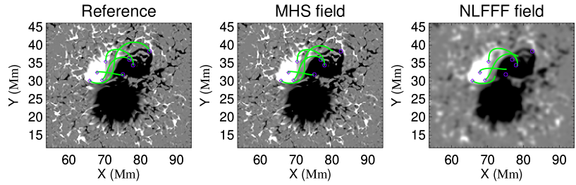
Figure 3: Selected field lines for test case in Zhu & Wiegelmann (2019). The start points marked with rhombus are the same in each panel. Circles in each panel mark end points of the referenced field lines. Magnetogram of the NLFFF model is smoother than other two panels due to force-free preprocessing procedure (Wiegelmann et al., 2006). (a) Reference model (Cheung et al., 2019), (b) MHS model implemented by Zhu & Wiegelmann (2018, 2019), (c) NLFFF model implemented by Wiegelmann (2004)

.

The analytical MHS models have the advantage of leading to linear equations, which are computationally very cheap. However, one has to make a number of assumptions to derive the analytical solution, which limit the applicability of this kind of the MHS models to some extent. The numerical MHS models basically make no assumptions (except assuming a static state), and therefore are capable of modeling strong current concentrations locally which naturally leads to a nonlinear mathematical problem. However, the numerical MHS models are found to be really computationally expensive. Gilchrist et al. (2016) pointed out that more tracing steps (two in MHS case while only one in NLFFF case) and more stages involved in a single iteration slow down the MHS code significantly compared with the Grad-Rubin NLFFF code. The problem seems even worse in the optimization MHS code, which is 50 times slower than the optimization NLFFF code. The main reason is because there is a big difference in magnitude of the plasma parameters (e.g., pressure) through out the computational box and the code converges slowly. Recently, to reduce computational time, Zhu & Wiegelmann (2022) restricted the MHS extrapolation box to the non-force-free layer and then used the chromospheric vector magnetogram deduced from the MHS extrapolation to perform the NLFFF extrapolation. The combined approach reaches the accuracy of the MHS extrapolation and is moderately more efficient (still 7 times slower than the optimization NLFFF code).

The MHS models require high spatial resolution boundary conditions as input to resolve the fine structures in the solar lower atmosphere. While the spatial resolution of the observation is very high, the FOV usually limits to part of the observed active region (e.g., SUNRISE/IMaX covers a region of 37$\times$37 Mm with a pixel spacing of 40 km). To make the vector magnetogram to cover the entire active region which is necessary for a successful extrapolation by including more electric currents (De Rosa et al., 2009), one has to either embed the high-resolution magnetogram into the lower one (Wiegelmann et al., 2017; Zhu et al., 2020) or perform mosaic observations (Vissers et al., 2021). The combined magnetogram usually has a large number of grid points (e.g., up to 2000$\times$2000 even for a moderate active region with a FOV of 80$\times$80 Mm) which is also an challenge for extrapolations in terms of computing time and usage of computational resources. Implementation of MHS codes on massive parallel computer is needed currently or, at least, in the near future.

It is also worth noting that extrapolations with multiple observational data sets could improve the result dramatically. Methods that take advantage of combining magnetograms and EUV images have also been developed by Malanushenko et al. (2009, 2012) using a Quasi-Grad-Rubin method (QGR), Aschwanden (2013, 2016) based on vertical-current-approximation (VCA-NLFFF), and Chifu et al. (2015, 2017) based on the optimization method (S-NLFFF). An issue that should be kept in mind when using multiple data sets is that providing all observations might overdetermines the boundary condition, and no solution can be obtained. Both QGR and VCA-NLFFF use normal component of the photospheric magnetic field, which rely on a well-posed boundary value problem. S-NLFFF uses full magnetic vector as boundary condition, which is overdetermined. However, S-NLFFF specifies measurement errors and, as a result, the optimal solution is allowed to deviate from observation within the errors. In the case of the MHS extrapolation, using multiple observations is also a promising way to get improved results. Vissers et al. (2021) investigated the similarity between the chromospheric magnetic fields inferred from direct inversion and the MHS extrapolation. They found the latter underestimates the transverse field strength as well as the amount of structure in the chromosphere. Therefore, more constraints (e.g., chromospheric magnetic field inversion at reliable sites) may be included in the MHS extrapolation in future developments, and it seems not too difficult for the optimization approach to do so by just adding additional terms in the functional to be minimized.

In numerical MHS models, the Grad-Rubin method uses well-defined boundary conditions made of $B_{n}$ in both polarities and $p$ and $J_{n}$ in one, which will not violate the “hyperbolic” transport properties of $p$ and field-aligned component of the current. However, both optimization method and MHD relaxation method require the full magnetic vector and $p$ in both polarities as input. They obviously overspecify boundary conditions if a $T(\textbf{r})$ distribution everywhere in the computational box is prescribed. However, the boundary issue can be somewhat relieved by allowing deviation of the boundary conditions from observation within measurement error.

So far, most of the efforts made regarding the MHS extrapolation concentrate on the model developments including testing and validating of the method with known reference models. Results, with these tests, have shown that the MHS extrapolation is capable of reconstructing field lines with higher accuracy (see figure 3). However, applications of the MHS extrapolation to the observational data, from which we could learn new physics, are not as commonly seen as those of the NLFFF extrapolation. One of the reasons is that there are still some problems to be solved to make the MHS extrapolation as reliable as the NLFFF extrapolation in applying to solar data routinely. Another reason is that we do not have sufficient photospheric magnetic field measurements with sufficiently high spatial resolution ($\leq 100$ km). However, high-resolution measurements (e.g. with DKIST) are improving rapidly, which offer great opportunities to develop the MHS extrapolation. The MHS equilibrium also serves as a better initial condition than the NLFFF for the time-dependent MHD simulations.

References

- Régnier (2013) Régnier S. Magnetic Field Extrapolations into the Corona: Success and Future Improvements. Sol Phys, 2013, 288: 481-505
- Guo et al. (2017) Guo Y, Cheng X, Ding M D. Origin and structures of solar eruptions II: Magnetic modeling. Sci China Earth Sci, 2017, 60: 1408-1439
- Wiegelmann & Sakurai (2021) Wiegelmann T, Sakurai T. Solar force-free magnetic fields. Living Rev Sol Phys, 2021, 18: 1
- Gary (2001) Gary G A. Plasma Beta above a Solar Active Region: Rethinking the Paradigm. Sol Phys, 2001, 203: 71-86
- Shafranov (1958) Shafranov V D. On Magnetohydrodynamical Equilibrium Configurations. Sov J Exp Theor Phys, 1958, 6: 545
- Boozer (2004) Boozer A H. Physics of magnetically confined plasmas. Rev Mod Phys, 2004, 76: 1071
- Hesse & Birn (1993) Hesse M, Birn J. Three-dimensional magnetotail equilibria by numerical relaxation techniques. J Geophys Res, 1993, 98: 3973-3982
- Scherrer et al. (2012) Scherrer P H, Schou J, Bush R I, et al. The Helioseismic and Magnetic Imager (HMI) Investigation for the Solar Dynamics Observatory (SDO). Sol Phys, 2012, 275: 207-227
- Keil et al. (2011) Keil S L, Rimmele T R, Wagner J, et al. ATST: The Largest Polarimeter. Solar Polarization 6. Proceedings of a conference held in Maui, Hawaii, USA, 2011, 437: 319
- Parker (1972) Parker E N. Topological Dissipation and the Small-Scale Fields in Turbulent Gases. Astrophys J, 1972, 174: 499
- Dungey (1953) Dungey J W. A family of solutions of the magneto-hydrostatic problem in a conducting atmosphere in a gravitational field. Mon Notices Royal Astron Soc, 1953, 113: 180-187
- Low (1975) Low B C. Nonisothermal magnetostatic equlibria in a uniform gravity field. I. Mathematical formulation. Astrophys J, 1975, 197: 251-255
- Hundhausen et al. (1981) Hundhausen J R, Hundhausen A J, Zweibel E G. Magnetostatic atmospheres in a spherical geometry and their application to the solar corona. J Geophys Res, 1981, 86: 11117-11126
- Uchida & Low (1981) Uchida Y, Low B C. Equilibrium configuration of the magnetosphere of a star loaded with accreted magnetized mass. J Astrophys Astron, 1981, 2: 405-419
- Amari & Aly (1989) Amari T, Aly J J. Two-dimensional isothermal magnetostatic equilibria in a gravitational field. I - Unsheared equilibria. Astron Astrophys, 1989, 208: 361-373
- Low (1982) Low B C. Magnetostatic atmospheres with variations in three dimensions. Astrophys J, 1982, 263: 952-969
- Low (1984) Low B C. Three-dimensional magnetostatic atmospheres - Magnetic field with vertically oriented tension force. Astrophys J, 1984, 277: 415-421
- Hu et al. (1983) Hu W R, Hu Y Q, Low B C. Non Axisymmetric Magnetostatic Equilibrium - Part One - a Perturbation Theory. Sol Phys, 1983, 83: 195-205
- Low (1985) Low B C. Three-dimensional structures of magnetostatic atmospheres. I - Theory. Astrophys J, 1985, 293: 31-43
- Schmidt (1964) Schmidt H U. On the Observable Effects of Magnetic Energy Storage and Release Connected With Solar Flares. The Physics of Solar Flares, Proceedings of the AAS-NASA Symposium, 1964, 50: 107
- Chiu & Hilton (1977) Chiu Y T, Hilton H H. Exact Green’s function method of solar force-free magnetic-field computations with constant alpha . I. Theory and basic test cases. Astrophys J, 1977, 212: 873-885
- Bogdan & Low (1986) Bogdan T J, Low B C. The Three-dimensional Structure of Magnetostatic Atmospheres. II. Modeling the Large-Scale Corona. Astrophys J, 1986, 306: 271
- Low (1991) Low B C. Three-dimensional Structures of Magnetostatic Atmospheres. III. A General Formulation. Astrophys J, 1991, 370: 427
- Osherovich (1985a) Osherovich V A. Quasi-potential magnetic fields in stellar atmospheres. I - Static model of magnetic granulation. Astrophys J, 1985, 298: 235-239
- Osherovich (1985b) Osherovich V A. The eigenvalue approach in modelling solar magnetic structures. Aust J Phys, 1985, 38: 975-980
- Low (1992) Low B C. Three-dimensional Structures of Magnetostatic Atmospheres. IV. Magnetic Structures over a Solar Active Region. Astrophys J, 1992, 399: 300
- Neukirch (1995) Neukirch T. On self-consistent three-dimensional analytic solutions of the magnetohydrostatic equations.. Astron Astrophys, 1995, 301: 628
- Petrie & Neukirch (2000) Petrie G J, Neukirch T. The Green’s function method for a special class of linear three-dimensional magnetohydrostatic equilibria. Astron Astrophys, 2000, 356: 735-746
- Neukirch & Wiegelmann (2019) Neukirch T, Wiegelmann T. Analytical Three-dimensional Magnetohydrostatic Equilibrium Solutions for Magnetic Field Extrapolation Allowing a Transition from Non-force-free to Force-free Magnetic Fields. Sol Phys, 2019, 294: 171
- Neukirch (1997) Neukirch T. Nonlinear self-consistent three-dimensional arcade-like solutions of the magnetohydrostatic equations. Astron Astrophys, 1997, 325: 847-856
- Neukirch & Rastätter (1999) Neukirch T, Rastätter L. A new method for calculating a special class of self-consistent three-dimensional magnetohydrostatic equilibria. Astron Astrophys, 1999, 348: 1000-1004
- Nakagawa & Raadu (1972) Nakagawa Y, Raadu M A., On Practical Representation of Magnetic Field. Sol Phys, 1972, 25: 127-135
- MacTaggart et al. (2013) MacTaggart D, Elsheikh A, McLaughlin J A, et al. Non-symmetric magnetohydrostatic equilibria: a multigrid approach. Astron Astrophys, 2013, 556: A40
- Neukirch (2009) Neukirch T. Three-dimensional analytical magnetohydrostatic equilibria of rigidly rotating magnetospheres in cylindrical geometry. Geophys Astrophys Fluid Dyn, 2009, 103: 535-547
- Al-Salti & Neukirch (2010) Al-Salti N, Neukirch T. Three-dimensional solutions of the magnetohydrostatic equations: Rigidly rotating magnetized coronae in spherical geometry. Astron Astrophys, 2010, 520: A75
- Al-Salti et al. (2010) Al-Salti N, Neukirch T, Ryan R. Three-dimensional solutions of the magnetohydrostatic equations: rigidly rotating magnetized coronae in cylindrical geometry. Astron Astrophys, 2010, 514: A38
- Wilson & Neukirch (2018) Wilson F, Neukirch T. Three-dimensional solutions of the magnetohydrostatic equations for rigidly rotating magnetospheres in cylindrical coordinates. Geophys Astrophys Fluid Dyn, 2018, 112: 74-95
- Low (1993) Low B C. Three-dimensional Structures of Magnetostatic Atmospheres. V. Coupled Electric Current Systems. Astrophys J, 1993, 408: 689
- Choe & Minhwan (2013) Choe G S, Minhwan Jang M. Magnetic Flux-Current Surfaces of Magnetohydrostatic Equilibria. J Korean Astron Soc, 2013, 46: 261-268
- Aulanier et al. (1998) Aulanier G, Démoulin P, Schmieder B, et al. Tang, Magnetohydrostatic Model of a Bald-Patch Flare. Sol Phys, 1998, 183: 369-388
- Wiegelmann et al. (2015) Wiegelmann T, Neukirch T, Nickeler D H, et al. Magneto-static Modeling of the Mixed Plasma Beta Solar Atmosphere Based on Sunrise/IMaX Data. Astrophys J, 2015, 815: 10
- Wiegelmann et al. (2017) Wiegelmann T, Neukirch T, Nickeler D H, et al. Magneto-static Modeling from Sunrise/IMaX: Application to an Active Region Observed with Sunrise II. Astrophys J, Suppl Ser, 2017, 229: 18
- Solanki et al. (2017) Solanki S K, Riethmüller T L, Barthol P, et al. The Second Flight of the Sunrise Balloon-borne Solar Observatory: Overview of Instrument Updates, the Flight, the Data, and First Results. Astrophys J, Suppl Ser, 2017, 229: 2
- Hagino & Sakurai (2004) Hagino M, Sakurai T. Latitude Variation of Helicity in Solar Active Regions. Publ Astron Soc Jpn, 2004, 56: 831-843
- Aulanier & Demoulin (1998) Aulanier G, Demoulin P. 3-D magnetic configurations supporting prominences. I. The natural presence of lateral feet. Astron Astrophys, 1998, 329: 1125-1137
- Molodensky (1969) Molodensky M M. Integral Properties of Force-Free Fields. Sov Astron, 1969, 12: 585
- Molodensky (1974) Molodensky M M. Equilibrium and Stability of Force-Free Magnetic Field. Sol Phys, 1974, 39: 393-404
- Wiegelmann et al. (2006) Wiegelmann T, Inhester B, Sakurai T. Preprocessing of Vector Magnetograph Data for a Nonlinear Force-Free Magnetic Field Reconstruction. Sol Phys, 2006, 233: 215-232
- Low (2005) Low B C. Three-dimensional Structures of Magnetostatic Atmospheres. VII. Magnetic Flux Surfaces and Boundary Conditions. Astrophys J, 2005, 625: 451
- Aly (1989) Aly J J. On the Reconstruction of the Nonlinear Force-Free Coronal Magnetic Field from Boundary Data. Sol Phys, 1989, 120: 19-48
- Fletcher et al. (2001) Fletcher L, López Fuentes M C, Mandrini C H, Schmieder B, et al. A Relationship Between Transition Region Brightenings, Abundances, and Magnetic Topology. Sol Phys, 2001, 203: 255-287
- Mandrini et al. (2002) Mandrini C H, Démoulin P, Schmieder B, et al. The role of magnetic bald patches in surges and arch filament systems. Astron Astrophys, 2002, 391: 317-329
- Aulanier et al. (1999) Aulanier G, Démoulin P, Mein N, et al. 3-D magnetic configurations supporting prominences. III. Evolution of fine structures observed in a filament channel. Astron Astrophys, 1999, 342: 867-880
- Dudík et al. (2008) Dudík J, Aulanier G, Schmieder B, et al. Topological Departures from Translational Invariance along a Filament Observed by THEMIS. Sol Phys, 2008, 248: 29-50
- Martínez Pillet et al. (2011) Martínez Pillet V, Del Toro Iniesta J C, Álvarez-Herrero A, et al. The Imaging Magnetograph eXperiment (IMaX) for the Sunrise Balloon-Borne Solar Observatory. Sol Phys, 2001, 268: 57-102
- Solanki et al. (2010) Solanki S K, Barthol P, Danilovic S, et al. SUNRISE: Instrument, Mission, Data, and First Results. Astrophys J Lett, 2010. 723: L127
- Jafarzadeh et al. (2017) Jafarzadeh S, Rutten R J, Solanki S K, et al. Slender Ca II H Fibrils Mapping Magnetic Fields in the Low Solar Chromosphere. Astrophys J, Suppl Ser, 2017, 229: 11
- Mackay & Yeates (2012) Mackay D H, Yeates A R. The Sun’s Global Photospheric and Coronal Magnetic Fields: Observations and Models. Living Rev Sol Phys, 2012, 9: 6
- Bagenal & Gibson (1991) Bagenal F, Gibson S. Modeling the large-scale structure of the solar corona. J Geophys Res, 1991, 96: 17663-17674
- Gibson & Bagenal (1995) Gibson S E, Bagenal F. Large-scale magnetic field and density distribution in the solar minimum corona. J Geophys Res, 1995, 100: 19865-19880
- Gibson et al. (1996) Gibson S E, Bagenal F, Low B C. Current sheets in the solar minimum corona. J Geophys Res, 1996, 101: 4813-4823
- Zhao & Hoeksema (1993) Zhao X P, Hoeksema J T. Unique Determination of Model Coronal Magnetic Fields Using Photospheric Observations. Sol Phys, 1993, 143: 41-48
- Zhao & Hoeksema (1994) Zhao X P, Hoeksema J T. A Coronal Magnetic Field Model with Horizontal Volume and Sheet Currents. Sol Phys, 1994, 151: 91-105
- Zhao & Hoeksema (1995) Zhao X P, Hoeksema J T. Predicting the heliospheric magnetic field using the current sheet-source surface model. Adv Space Res, 1994, 16: 181-184
- Schatten (1971) Schatten K H. Current sheet magnetic model for the solar corona. Cosmic Electrodyn, 1971, 2: 232-245
- Ambrož et al. (2009) Ambrož P, Druckmüller M, Galal A A. 3D Coronal Structures and Magnetic Field During the Total Solar Eclipse of 29 March 2006. Sol Phys, 2009, 258: 243-265
- Yeates et al. (2018) Yeates A R, Amari T, Contopoulos I, et al. Global Non-Potential Magnetic Models of the Solar Corona During the March 2015 Eclipse. Space Sci Rev, 2018, 214: 99
- Zhao et al. (2000) Zhao X P, Hoeksema J T, Scherrer P H. Modeling the 1994 April 14 Polar Crown SXR Arcade Using Three-Dimensional Magnetohydrostatic Equilibrium Solutions. Astrophys J, 2000, 538: 932
- Rudenko (2001) Rudenko G V. A constructing method for a self-consistent three-dimensional solution of the magnetohydrostatic equations using full-disk magnetogram data. Sol Phys, 2001, 198: 279-287
- Ruan et al. (2008) Ruan P, Wiegelmann T, Inhester B, et al. A first step in reconstructing the solar corona self-consistently with a magnetohydrostatic model during solar activity minimum. Astron Astrophys, 2008, 481: 827-834
- Wiegelmann & Neukirch (2006) Wiegelmann T, Neukirch T. An optimization principle for the computation of MHD equilibria in the solar corona. Astron Astrophys, 2006, 457: 1053-1058
- Zhu & Wiegelmann (2018) Zhu X S, Wiegelmann T. On the Extrapolation of Magnetohydrostatic Equilibria on the Sun. Astrophys J, 2018, 866: 130
- Zhu & Wiegelmann (2019) Zhu X S, Wiegelmann T. Testing magnetohydrostatic extrapolation with radiative MHD simulation of a solar flare. Astron Astrophys, 2019, 631: A162
- Zhu et al. (2013) Zhu X S, Wang H N, Du Z L, et al. Forced Field Extrapolation: Testing a Magnetohydrodynamic (MHD) Relaxation Method with a Flux-rope Emergence Model. Astrophys J, 2013, 768: 119
- Miyoshi et al. (2020) Miyoshi T, Kusano K, Inoue S. A Magnetohydrodynamic Relaxation Method for Non-force-free Magnetic Field in Magnetohydrostatic Equilibrium. Astrophys J, Suppl Ser, 2020, 247: 6
- Gilchrist & Wheatland (2013) Gilchrist S A, Wheatland M S. A Magnetostatic Grad-Rubin Code for Coronal Magnetic Field Extrapolations. Sol Phys, 2013, 282: 283-302
- Gilchrist et al. (2016) Gilchrist S A, Braun D C, Barnes G. A Fixed-point Scheme for the Numerical Construction of Magnetohydrostatic Atmospheres in Three Dimensions. Sol Phys, 2016, 291: 3583-3603
- Stern (1970) Stern D P. Euler Potentials. Am J Phys, 1970, 38: 494
- Stern (1976) Stern D P. Representation of magnetic fields in space. Rev Geophys, 1976, 14: 199-214
- Schindler (2006) Schindler K. Physics of Space Plasma Activity. Cambridge University Press, 2006, 522
- Wheatland et al. (2000) Wheatland M S, Sturrock P A, Roumeliotis G. An Optimization Approach to Reconstructing Force-free Fields. Astrophys J, 2000, 540: 1150
- Low & Lou (1990) Low B C, Lou Y Q. Modeling Solar Force-free Magnetic Fields. Astrophys J, 1990, 352: 343
- Wiegelmann et al. (2007) Wiegelmann T, Neukirch T, Ruan P, et al. Optimization approach for the computation of magnetohydrostatic coronal equilibria in spherical geometry. Astron Astrophys, 2007, 475: 701-706
- Kageyama & Sato (2004) Kageyama A, Sato T. “Yin-Yang grid”: An overset grid in spherical geometry. Geochem Geophys Geosystems, 2004, 5: Q09005
- Wiegelmann (2004) Wiegelmann T. Optimization code with weighting function for the reconstruction of coronal magnetic fields. Sol Phys, 2004, 219: 87-108
- Wiegelmann et al. (2012) Wiegelmann T, Thalmann J K, Inhester B, et al. How Should One Optimize Nonlinear Force-Free Coronal Magnetic Field Extrapolations from SDO/HMI Vector Magnetograms? Sol Phys, 2012, 281: 37-51
- Cheung et al. (2019) Cheung M C, Rempel M, Chintzoglou G, et al. A comprehensive three-dimensional radiative magnetohydrodynamic simulation of a solar flare. Nat Astron, 2019, 3: 160-166
- Zhu et al. (2020) Zhu X S, Wiegelmann T, Solanki S K. Magnetohydrostatic modeling of AR11768 based on a SUNRISE/IMaX vector magnetogram. Astron Astrophys, 2020, 640: A103
- Hou et al. (2021) Hou Z Y, Tian H, Chen H C, et al. Formation of Solar Quiescent Coronal Loops through Magnetic Reconnection in an Emerging Active Region. Astrophys J, 2021, 915: 39
- Jafarzadeh et al. (2021) Jafarzadeh S, Wedemeyer S, Fleck B, et al. An overall view of temperature oscillations in the solar chromosphere with ALMA. Philos Trans Royal Soc A, 2021, 379: 20200174
- Mikic et al. (1988) Mikic Z, Barnes D C, Schnack D D. Dynamical Evolution of a Solar Coronal Magnetic Field Arcade. Astrophys J, 1988, 328: 830
- Roumeliotis (1996) Roumeliotis G. The “Stress-and-Relax” Method for Reconstructing the Coronal Magnetic Field from Vector Magnetograph Data. Astrophys J, 1996, 473: 1095
- McClymont et al. (1997) McClymont A N, Jiao L, Mikic Z. Problems and Progress in Computing Three-Dimensional Coronal Active Region Magnetic Fields from Boundary Data. Sol Phys, 1997, 174: 191-218
- Valori et al. (2005) Valori G, Kliem B, Keppens R. Extrapolation of a nonlinear force-free field containing a highly twisted magnetic loop. Astron Astrophys, 2005, 433: 335-347
- Jiang & Feng (2012) Jiang C W, Feng X S, Xiang C Q. A New Code for Nonlinear Force-free Field Extrapolation of the Global Corona. Astrophys J, 2012, 755: 62
- Guo et al. (2016) Guo Y, Xia C, Keppens R, et al. Magneto-frictional Modeling of Coronal Nonlinear Force-free Fields. I. Testing with Analytic Solutions. Astrophys J, 2016, 828: 82
- Zhu et al. (2016) Zhu X S, Wang H N, Du Z L, et al. Forced Field Extrapolation of the Magnetic Structure of the H fibrils in the Solar Chromosphere. Astrophys J, 2016, 826: 51
- Wang et al. (2016) Wang R, Liu Y D, Zimovets I, et al. Sympathetic Solar Filament Eruptions. Astrophys J Lett, 2016, 827: L12
- Zhao et al. (2017) Zhao J, Schmieder B, Li H, et al. Observational Evidence of Magnetic Reconnection for Brightenings and Transition Region Arcades in IRIS Observations. Astrophys J, 2017, 836: 52
- Tian et al. (2018) Tian H, Zhu X S, Peter H, et al. Magnetic Reconnection at the Earliest Stage of Solar Flux Emergence. Astrophys J, 2018, 854: 174
- Chen et al. (2019) Chen Y J, Tian H, Zhu X S, et al. Solar ultraviolet bursts in a coordinated observation of IRIS, Hinode and SDO. Sci China Tech Sci, 2019, 62: 1555-1564
- Zhu et al. (2017) Zhu X S, Wang H N, Cheng X, et al. A Solar Blowout Jet Caused by the Eruption of a Magnetic Flux Rope. Astrophys J Lett, 2017, 844: L20
- Song et al. (2018) Song Y L, Guo Y, Tian H, et al. Observations of a White-light Flare Associated with a Filament Eruption. Astrophys J, 2018, 854 64
- Miao et al. (2018) Miao Y H, Liu Y, Li H B, et al. A Blowout Jet Associated with One Obvious Extreme-ultraviolet Wave and One Complicated Coronal Mass Ejection Event. Astrophys J, 2018, 869: 39
- Joshi et al. (2019) Joshi N C, Zhu X S, Schmieder B, et al. Generalization of the Magnetic Field Configuration of Typical and Atypical Confined Flares. Astrophys J, 2019, 871: 165
- Song et al. (2020) Song Y L, Tian H, Zhu X S, et al. A White-light Flare Powered by Magnetic Reconnection in the Lower Solar Atmosphere. Astrophys J Lett, 2020, 893: L13
- Fu et al. (2020) Fu H, Harrison R A, Davies J A, et al. The High Helium Abundance and Charge States of the Interplanetary CME and Its Material Source on the Sun. Astrophys J Lett, 2020, 900: L18
- Grad & Rubin (1958) Grad H, Rubin H. Hydromagnetic equilibria and force-free fields. In: Peaceful uses of atomic energy. Theoretical and experimental aspects of controlled nuclear fusion. 1958, 31: 190
- Sakurai (1981) Sakurai T. Calculation of force-free magnetic field with non-constant . Sol Phys, 1981, 69: 343-359
- Amari et al. (1999) Amari T, Boulmezaoud T Z, Mikic Z. An iterative method for the reconstructionbreak of the solar coronal magnetic field. I. Method for regular solutions. Astron Astrophys, 1999, 350: 1051-1059
- Wheatland (2007) Wheatland M S. Calculating and Testing Nonlinear Force-Free Fields. Sol Phys, 2007, 245: 251-262
- Low (1980) Low B C. Exact Static Equilibrium of Vertically Oriented Magnetic Flux Tubes - Part One - the Schluter-Temesvary Sunspot. Sol Phys, 1980, 67: 57-77
- Wheatland (2006) Wheatland M S. A Fast Current-Field Iteration Method for Calculating Nonlinear Force-Free Fields. Sol Phys, 2006, 238: 29-39
- Zwingmann et al. (1985) Zwingmann W, Schindler K, Birn J. On Sheared Magnetic Field Structures Containing Neutral Points. Sol Phys, 1985, 99: 133-143
- Zwingmann (1987) Zwingmann W. Theoretical study of onset conditions for solar eruptive processes. Sol Phys, 1987, 111: 309-331
- Platt & Neukirch (1994) Platt U, Neukirch T. Theoretical Study of Onset Conditions for Solar Eruptive Processes - Influence of the Boundaries. Sol Phys, 1994, 153: 287-306
- Romeou & Neukirch (1999) Romeou Z, Neukirch T. Self-consistent Models of Solar Magnetic Structures in Three Dimensions, in: Magnetic Fields and Solar Processes, Proceedings of the 9th European Meeting of Solar Physics, 1999, SP-448: 871
- Romeou & Neukirch (2002) Romeou Z, Neukirch T. On the application of numerical continuation methods to the calculation of magnetostatic equilibria. J Atmos Sol Terr Phys, 2002, 64: 639-644
- Mathews et al. (2021) Mathews N H, Flyer N, Gibson S E. Solving 3D Magnetohydrostatics with RBF-FD: Applications to the Solar Corona. arXiv, 2021, arXiv:2112.04561
- Gibson & Low (1998) Gibson S E, Low B C. A Time-Dependent Three-Dimensional Magnetohydrodynamic Model of the Coronal Mass Ejection. Astrophys J, 1998, 493: 460
- Aly (1984) Aly J J, On some properties of force-free magnetic fields in infinite regions of space. Astrophys J, 1984, 283: 349-362
- Metcalf et al. (1995) Metcalf T R, Jiao L, McClymont A N, et al. Is the Solar Chromospheric Magnetic Field Force-free? Astrophys J, 1995 439: 474
- Moon et al. (2002) Moon Y J, Choe G S, Yun H S, et al. Force-Freeness of Solar Magnetic Fields in the Photosphere. Astrophys J, 2002, 568: 422
- Tiwari (2012) Tiwari S K. On the Force-free Nature of Photospheric Sunspot Magnetic Fields as Observed from Hinode (SOT/SP). Astrophys J, 2012, 744: 65
- Liu et al. (2013) Liu S, Su J T, Zhang H Q, et al. A Statistical Study on Force-Freeness of Solar Magnetic Fields in the Photosphere. Publ Astron Soc Aust, 2013, 30: e005
- Metcalf et al. (2008) Metcalf T R, De Rosa M L, Schrijver C J, et al. Nonlinear Force-Free Modeling of Coronal Magnetic Fields. II. Modeling a Filament Arcade and Simulated Chromospheric and Photospheric Vector Fields. Sol Phys, 2008, 247: 269-299
- Zhu et al. (2020) Zhu X S, Wiegelmann T, Inhester B. Preprocessing of vector magnetograms for magnetohydrostatic extrapolations. Astron Astrophys, 2020, 644: A57
- Zhu & Wiegelmann (2022) Zhu X S, Wiegelmann T. Toward a fast and consistent approach to modeling solar magnetic fields in multiple layers. Astron Astrophys, 2022, 658: A37
- De Rosa et al. (2009) De Rosa M L, Schrijver C J, Barnes G, et al. A Critical Assessment of Nonlinear Force-Free Field Modeling of the Solar Corona for Active Region 10953. Astrophys J, 2009, 696: 1780
- Vissers et al. (2021) Vissers G J, Danilovic S, Zhu X, J. et al. Active region chromospheric magnetic fields. arXiv, 2021, arXiv:2109.02943
- Malanushenko et al. (2009) Malanushenko A, Longcope D W, McKenzie D E. Reconstructing the Local Twist of Coronal Magnetic Fields and the Three-Dimensional Shape of the Field Lines from Coronal Loops in Extreme-Ultraviolet and X-Ray Images. Astrophys J, 2009, 707: 1044
- Malanushenko et al. (2012) Malanushenko A, Schrijver C J, DeRosa M L, et al. Guiding Nonlinear Force-free Modeling Using Coronal Observations: First Results Using a Quasi-Grad-Rubin Scheme. Astrophys J, 2012, 756: 153
- Aschwanden (2013) Aschwanden M J. A Nonlinear Force-Free Magnetic Field Approximation Suitable for Fast Forward-Fitting to Coronal Loops. I. Theory. Sol Phys, 2013, 287: 323-344
- Aschwanden (2016) Aschwanden M J, The Vertical-current Approximation Nonlinear Force-free Field Code—Description, Performance Tests, and Measurements of Magnetic Energies Dissipated in Solar Flares. Astrophys J, Suppl Ser, 2016, 224: 25
- Chifu et al. (2015) Chifu I, Inhester B, Wiegelmann T. Coronal magnetic field modeling using stereoscopy constraints. Astron Astrophys, 2015, 577: A123
- Chifu et al. (2017) Chifu I, Wiegelmann T, Inhester B. Nonlinear Force-free Coronal Magnetic Stereoscopy. Astrophys J, 2017, 837: 10