Cross-Modality High-Frequency Transformer for
MR Image Super-Resolution
Abstract.
Improving the resolution of magnetic resonance (MR) image data is critical to computer-aided diagnosis and brain function analysis. Higher resolution helps to capture more detailed content, but typically induces to lower signal-to-noise ratio and longer scanning time. To this end, MR image super-resolution has become a widely-interested topic in recent times. Existing works establish extensive deep models with the conventional architectures based on convolutional neural networks (CNN). In this work, to further advance this research field, we make an early effort to build a Transformer-based MR image super-resolution framework, with careful designs on exploring valuable domain prior knowledge. Specifically, we consider two-fold domain priors including the high-frequency structure prior and the inter-modality context prior, and establish a novel Transformer architecture, called Cross-modality high-frequency Transformer (Cohf-T), to introduce such priors into super-resolving the low-resolution (LR) MR images. Experiments on two datasets indicate that Cohf-T achieves new state-of-the-art performance.
1. Introduction
Due to the superior capacity in capturing histopathological detail of soft tissues, magnetic resonance (MR) image becomes one of the most widely-used data in computer-aided diagnosis and brain function analysis. However, because of hardware and post-processing constraints, collecting MR images with higher resolution leads to lower signal-to-noise ratio or extends the scanning time (Plenge et al., 2012). For addressing this problem, one cost-effective way is to apply the super-resolution technology, which synthesizes the desired high-resolution (HR) MR image from the LR MR image.
The current main-stream technique for MR image super-resolution (SR) is based on convolutional neural networks (CNN) (Pham et al., 2017; Zhao et al., 2019). Although encouraging results are obtained by these CNN-based approaches, the intrinsic short-range reception mechanism is disadvantageous to the exploration of the global structure and long-range context information. This makes existing CNN-based MR image SR algorithms still sub-optimal for producing satisfactory results.
This paper makes an early effort to build a Transformer-based MR image super-resolution framework. In contrast to conventional CNN models, the Transformer model constituted by self-attention blocks has advantages in modeling the long-distance dependency (Vaswani et al., 2017). Such a network architecture is firstly evolved in natural language processing (NLP) and then achieves enormous success in vision tasks like image recognition (Dosovitskiy et al., 2020) and semantic segmentation (Strudel et al., 2021). It is also verified that Transformer-based modelling is effective in medical image segmentation (Chen et al., 2021a) and registration (Lee et al., 2019). Here, we leverage it to advance the research on the super-resolution of T2-weighted MR image (T2WI), a typical MR data used in clinics but costing a very long scanning time.
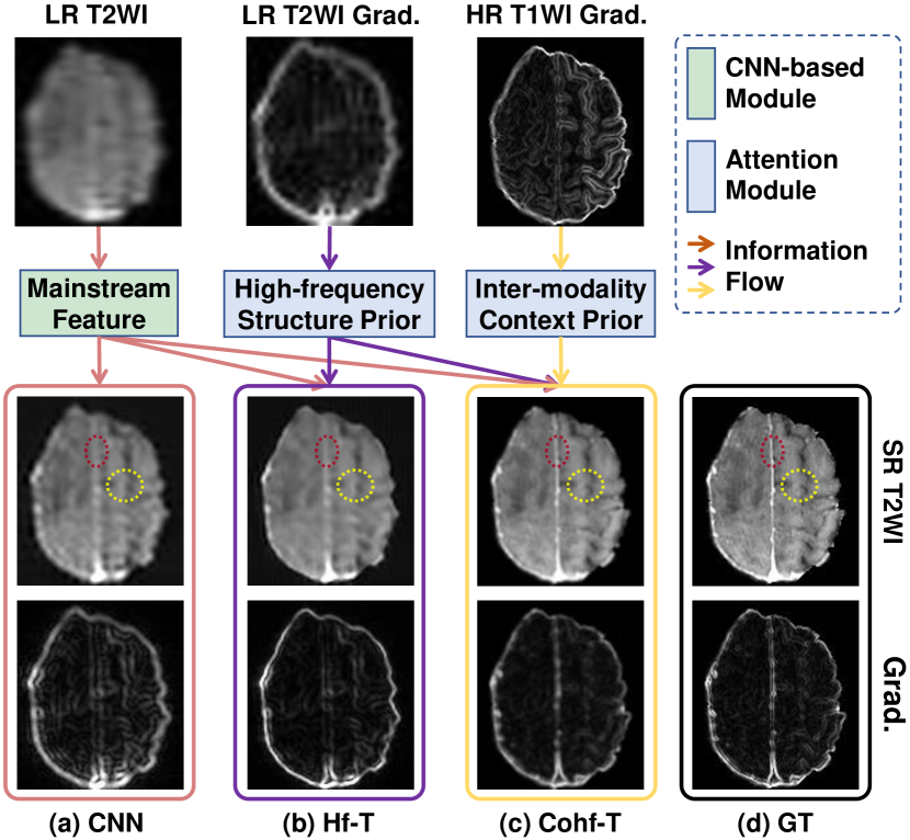
Existing transformer designs directly model self-attention in the original image domain. However, when implementing super-resolution on MR images, we find that the structure information held in the high-frequency domain would play a paramount role for model design as the organs appearing in the MR images usually share similar anatomical structures across persons, and the relation between different parts of the organ is regular (Cherukuri et al., 2019) (see Fig. 1). We term this as the high-frequency structure prior, and an example is provided to demonstrate the efficacy of the high-frequency structure prior in Fig. 1 (b). To this end, the transformer model designed in this work performs on the high-frequency image gradients rather than the conventionally used original image pixels.
Another important domain knowledge is that when processing LR T2WI data, the high-resolution T1-weighted images (T1WI) can be used to provide rich inter-modality context priors, as 1) the complementary morphological information (Zhang et al., 2020; Feng et al., 2021a; Zhang et al., 2021) captured by the T1WI can help infer the structural content of the T2WI , and 2) the acquisition of HR T1WI costs much less scanning time 111https://case.edu/med/neurology/NR/MRI%20Basics.htm. An example is also provided to demonstrate the efficacy of such inter-modality context prior in Fig. 1 (c).
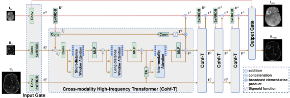
To explore the domain priors mentioned above, we propose a novel Transformer architecture called Cross-modality high-frequency Transformer (Cohf-T). A novel learning framework is set up for super-resolving LR T2WI under the guidance of gradient maps of both LR T2WI and HR T1WI. As shown in Fig. 2, our model has a main SR stream and a domain prior embedding stream, together with an input gate and an output gate. The domain prior embedding stream explores the high-frequency structure priors from the gradient map of LR T2WI and the inter-modality context from HR T1WI. Practically, both short-distance and long-distance dependencies are leveraged to explore high-frequency structure priors with the help of window attention modules. Considering there exists distribution shift between T2WI and T1WI, an adaptive instance normalization module is devised for aligning their features before performing the cross-modality attention. Additionally, a novel basic attention module that encloses both intra-head and inter-head correlations is proposed to improve the relation extraction capacity of our Transformer-based framework.
In summary, this work has three main contributions:
-
•
We make an early effort to establish a Transformer-based framework for super-resolving T2-weighted MR images, based on the proposed Cross-modality high-frequency Transformer (Cohf-T).
-
•
In Cohf-T, we introduce the high-frequency structure prior and inter-modality context prior by designing novel intra-modality window attention and inter-modality attention modules.
-
•
Comprehensive experiments on two MR image super-resolution benchmarks demonstrate that the proposed Cohf-T achieves new state-of-the-art performance.
2. Related Work
2.1. MR Image Super-Resolution
Improving the resolution of MR images is a long-lasting classical task in medical image analysis. Inspired by the rapid development in image super-resolution (Dong et al., 2015; Ledig et al., 2017; Zhang et al., 2018b; Wang et al., 2018; Fang et al., 2019; Niu et al., 2020; Fang et al., 2022) , CNN models have been the mainstream solutions for the MR image super-resolution (Chen et al., 2018; Pham et al., 2017; Zhao et al., 2019). According to the current studies (Ma et al., 2020; Yang et al., 2020; Lu et al., 2021), the low-frequency signals in MR data are relatively easy to reconstruct. In contrast, super-resolving the high-frequency signals, such as structures and textures, remains the main challenge.
Different from natural images, we can acquire MR images with multiple modalities via different imaging settings. A series of traditional algorithms (Rousseau et al., 2010; Jain et al., 2017) attempt to explore prior context information from T1-weighted MR images for super-resolving T2-weighted or spectroscopy MR images. (Iqbal et al., 2019; Feng et al., 2021a; Yang et al., 2021) further devise CNN models to exploit such inter-modality context information. However, directly fusing features of multiple modalities via convolutions with small kernels can not sufficiently leverage the inter-modality dependencies. To further advance this research field, we devise a novel Transformer-based super-resolution framework. The proposed framework can capture long-distance dependencies for involving the high-frequency structure prior and inter-modality context prior, which is beyond the exploration of the existing works.
2.2. Transformer for Vision Tasks
Transformer is primordially proposed for extracting long-distance relation context in NLP tasks (Vaswani et al., 2017). Recently, this technique has been extensively applied to computer vision tasks, considering it can help to make up the artifact of convolution that only local features can be captured with a limited kernel size (Chen et al., 2021b; Liang et al., 2021a; Dosovitskiy et al., 2020; Strudel et al., 2021; Peng et al., 2021; Liu et al., 2021).
Among the existing vision transformer models, self-attention (Buades et al., 2011; Liu et al., 2018; Zhu et al., 2020) and its variations, e.g., (Dai et al., 2019; Mei et al., 2021), are widely adopted to build the basic transformer block. For example, (Dai et al., 2019) exploits the second-order attention based on covariance normalization for feature enhancement in image super-resolution. In (Mei et al., 2021), the computation burden of the non-local operation is reduced by removing less informative correlations and constructing a sparse attention map. Transformer modules are also applied for tackling the multi-modal vision understanding tasks. Targeted at the multispectral object detection, (Qingyun et al., 2021) concatenates tokens from RGB and thermal modalities and then fuse them with symmetric attention modules. (Liang et al., 2021b) assigns specific modality embeddings to tokens from different modalities for solving the visible-infrared person re-identification task. Unlike these attention mechanisms, we introduce inter-head correlation in our attention modeling to further improve the feature interaction. Practically, three kinds of attention modules, namely short-distance window attention, long-distance window attention, and inter-modality attention, are incorporated in our transformer block.
3. Method
3.1. The Overall Learning Framework
This paper is targeted at super-resolving low-resolution (LR) T2-weighted image (T2WI) under the guidance of high-resolution (HR) T1-weighted image (T1WI). Specifically, given the main input image, namely a LR T2WI , we embed the high-frequency structure prior by calculating the gradient field for and define the gradient image as the structure reference input (denoted by , where is a constant and is set to ). The gradient of the HR T1WI (denoted by ) is regarded as an additional reference input for supplying inter-modality context information. and denote the height and width of , respectively. Then, a network architecture is built upon the cross-modality high-frequency transformer to predict the high-resolution T2-weighted image . denotes the upsampling ratio.
As shown in Fig. 2, our proposed framework is composed of two streams, including the main super-resolution stream (performing on the LR T2WI ) and the domain prior embedding stream, together with an input gate and an output gate. The intensity levels of T1WI are not directly related to those of T2WI, e.g., the inflammation appears to be dark in T1WI but bright in T2WI. On the other hand, the two kinds of images share similar structures. Thus, we extract the domain prior information with the LR T2WI gradient image and the HR T1WI gradient .
Input Gate. The input gate projects the input image data, including , , and to their corresponding primary features , , and through several convolutional layers and residual-in-residual dense blocks (RRDBs) (Wang et al., 2018).
Main Super-Resolution Stream. There are four stages in the main super-resolution stream. In each stage, five RRDBs are utilized for deriving more complicated latent features. For the -th stage, the extracted feature map is denoted by, . Then, is fed into a cross-modality high-frequency transformer (Cofh-T) block to interact with the high-frequency structure prior and inter-modality context prior, resulting in a domain prior embedding . A more detailed description of the Cohf-T block can be referred to in the next subsection. Extra structural information is extracted from via a convolution layer, resulting in . Then, a series of attention modules are employed to explore domain priors (namely ) from , , and . Finally, the prior-induced latent features of the current stage are produced via a shortcut connection: , where is a single-channel selection map inferred from , and ‘’ is the broadcast element-wise production.
Domain Prior Embedding Stream. This network stream which is composed of four cascaded Cohf-T blocks involves the and as inputs. In particular, for the -th Cohf-T block, we first combine previous prior features and additional structure features acquired from main stream features as 222For the first Cohf-T block, where .. Then, short-distance window attention and long-distance window attention are sequentially integrated to extract the high-frequency structure knowledge from . Next, together with inter-modality context prior features , the obtained attention features are further passed through an inter-modality attention module to generate the final domain prior embedding features .
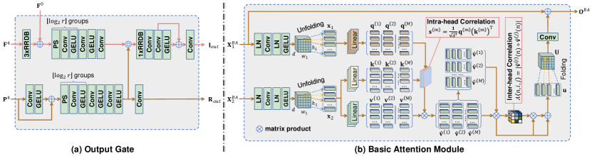
Output Gate. Based on the latent feature extracted from the main super-resolution stream and the domain prior embedding feature , an output gate is built up for jointly synthesizing high-resolution intensity and gradient images. The concrete architecture is shown in Fig. 3 (a).
Objective Function. We adopt the mean square error and structural similarity index measure to estimate the consistency between network predictions and the ground-truths. The following objective function is adopted for constraining the main prediction ,
| (1) |
where is a weighting coefficient, and represents the ground-truth HR T2WI. denotes the mean square error function, and denotes the function for calculating the structural similarity index measure.
3.2. Main Designs in Cofh-T
3.2.1. The Basic Attention Module
Different from the classic multi-head self-attention (MHSA) that is widely used in the existing transformer models (Vaswani et al., 2017; Dosovitskiy et al., 2020), we propose an alternative attention module as the basic unit of our model by taking both intra-head and inter-head correlations into consideration.
Given an input feature map and a reference context feature map ( might be equal to ), the target of the attention module is to extract the well-aligned context information from for enhancing the representation of . The whole calculation process is illustrated in Fig. 3 (b).
First, the layer normalization is applied to separately standardize and . A convolution accompanied with the other layer normalization and activation function GELU is utilized to embed into a -dimensional feature map. Afterwards, it is decomposed into local patches with size of and then arranged into patch-wise representation () via the unfolding operation which flattens local patches in the feature map into vectors. The similar process is utilized to transform to patch-wise representation , in which the size and stride of the convolution are both set to for registering the spatial dimensions of with those of , i.e., . groups of linear layers are used for generating query representations denoted by () from . Key representations (denoted by ) and value representations (denoted by ) are calculated by feeding into another linear layers.
Then, like the classic MHSA, intra-head correlation maps are calculated by the softmax function. The value at of the -th correlation map is estimated as,
| (3) |
where and represent the -th and the -th rows of and , respectively, and denotes the summation of all elements in the input tensor. These correlation maps estimate point-wise dependencies between two input feature maps from the same heads. With the correlation encoded by , we renew the value feature by, .
To explore the dependencies among different heads, we devise an inter-head correlation modelling algorithm. First, the inter-head correlation matrix is estimated as below,
| (4) |
where represents the -th row of . Then, the value features are combined with the inter-head correlation, resulting in . The -th row of is calculated as,
| (5) |
where is formed by stacking unit matrices with size of . Afterwards, -s are transformed into a tensor denoted by with the folding operation333The folding operation first expands the first dimension of into the spatial size of and then allocates the -dimensional feature vector of every point into a patch.. Finally, a convolution layer is adopted to post-process which is then fused into via a skip connection, deriving of an enhanced variant of (namely ).
3.2.2. Intra-modality Window Attention
Short-distance and long-distance windows are adopted to model the intra-modality dependency for restoring the high-resolution gradient field. In particular, the short-distance structure helps to amend local details such as noncontinuous boundaries with surrounding structure information. At the same time, the long-distance structure can leverage the repetition of textural and structural patterns to enhance the pixel-wise feature representation.
Inspired from (Liu et al., 2021), for acquiring the short-distance structure, we uniformly decompose the input feature map into compact windows with the size of as in Fig. 4 (a). Regarding the input feature map itself as the reference context features, the attention module in Section 3.2.1 is applied for enhancing features of every window. Afterward, the features are processed with a residual multi-layer perceptron (MLP) with a structure of ‘LN-Conv1x1-LN-GELU-Conv11’ (see Cohf-T in Fig. 2).
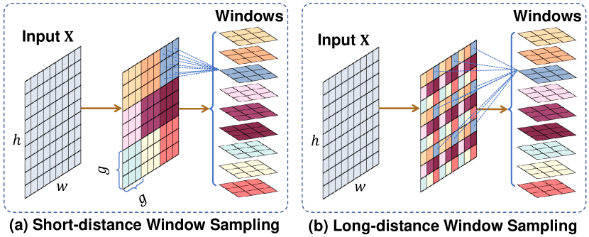
For extracting the long-distance dependency information, we propose to sample dilated windows from the input feature map (as shown in Fig. 4 (b)). The horizontal or vertical distance between neighboring points in each window is or . Then, the attention module, together with a residual MLP, is employed to enhance the features of each long-distance window. Once is larger than and , cascading the short-distance and long-distance window attention modules can efficiently extract context information from the full image. The former module aggregates the context information from the surrounding neighborhood, while the latter module involves the knowledge of all windows.
3.2.3. Inter-modality Attention
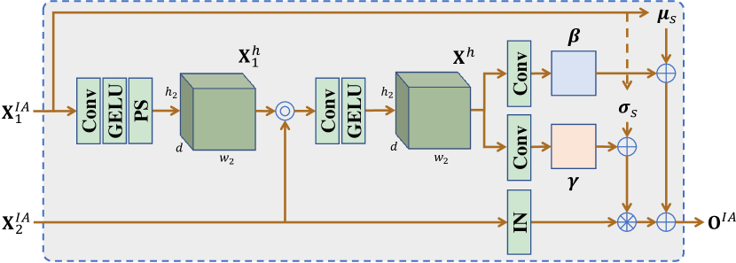
To involve the valuable inter-modality context information, we devise a cross-modality attention module within each Cohf-T block. Considering that there would be a large domain gap between the gradient fields of different modality data, directly injecting features of the T1 modality into those of the T2 modality would not be the optimal solution. Inspired from (Huang and Belongie, 2017; Lu et al., 2021), we adopt a point-wise adaptive instance normalization scheme to reduce the cross-modality representation gap as shown in Fig. 5.
Given the input feature maps and , the goal is to transfer the content of to a feature space that is finely aligned to . We estimate channel-wise mean and variance from , and then apply the instance normalization to standardize , resulting in as below,
| (6) |
To estimate and , we first align the height and width of with those of . Specifically, one convolution layer is first used to increase the channel number of to . Then, the resulted feature map is arranged to obtain via the pixel shuffle operation. Afterward, and are concatenated and compressed into a tensor (denoted by ) via one convolution layer. Point-wise affine parameters and are generated from with separate convolution layers. We can also calculate the channel-wise mean () and variance () vectors of . Then, the module outputs as the updating of :
| (7) |
The adaptive normalization in (Lu et al., 2021) calculates global affine parameters are calculated in each batch normalization layer. Our devised normalization to differs from it in the adoption of point-wise affine parameters, which model local distribution deviation more finely.
The adaptive normalization helps project features of T1 modality to get close to the feature distribution of the T2 modality. The feature streams of and correspond to and , respectively. Subsequently, the cross-modality attention is performed by using to generate the query features and using to create the key and value features. Then, another residual MLP is attached for further feature enhancement.
| Method | BraTS2018 dataset | IXI dataset | ||||||||||
|---|---|---|---|---|---|---|---|---|---|---|---|---|
| 2 | 3 | 4 | 2 | 3 | 4 | |||||||
| PSNR | SSIM | PSNR | SSIM | PSNR | SSIM | PSNR | SSIM | PSNR | SSIM | PSNR | SSIM | |
| Bicubic | 30.92 | 0.9198 | 28.19 | 0.9062 | 25.87 | 0.8388 | 29.71 | 0.9067 | 26.01 | 0.8070 | 24.32 | 0.7296 |
| RDN (Zhang et al., 2018b) | 34.57 | 0.9536 | 32.70 | 0.9324 | 30.92 | 0.9172 | 33.54 | 0.9435 | 31.02 | 0.9307 | 29.89 | 0.8998 |
| RCAN (Zhang et al., 2018a) | 34.82 | 0.9556 | 33.11 | 0.9310 | 30.88 | 0.9301 | 33.66 | 0.9422 | 30.79 | 0.9302 | 29.60 | 0.8936 |
| SAN (Dai et al., 2019) | 34.81 | 0.9544 | 32.91 | 0.9332 | 30.90 | 0.9281 | 34.31 | 0.9513 | 31.28 | 0.9401 | 29.59 | 0.8825 |
| CFSR (Tian et al., 2020) | 34.79 | 0.9566 | 32.66 | 0.9299 | 30.77 | 0.9290 | 34.24 | 0.9521 | 31.30 | 0.9320 | 29.78 | 0.8874 |
| HAN (Niu et al., 2020) | 35.01 | 0.9572 | 33.19 | 0.9351 | 31.03 | 0.9262 | 34.10 | 0.9480 | 31.36 | 0.9377 | 29.96 | 0.8993 |
| SRResCGAN (Umer et al., 2020) | 34.21 | 0.9492 | 33.00 | 0.9388 | 30.99 | 0.9048 | 34.02 | 0.9522 | 31.21 | 0.9388 | 30.24 | 0.8924 |
| SPSR (Ma et al., 2020) | 35.11 | 0.9585 | 33.32 | 0.9370 | 31.11 | 0.9264 | 34.47 | 0.9511 | 31.61 | 0.9382 | 30.47 | 0.8931 |
| SMSR (Wang et al., 2021) | 35.31 | 0.9601 | 33.62 | 0.9402 | 31.32 | 0.9342 | 34.77 | 0.9588 | 31.88 | 0.9477 | 30.36 | 0.9004 |
| NLSN (Mei et al., 2021) | 35.43 | 0.9655 | 33.99 | 0.9423 | 31.72 | 0.9321 | 34.51 | 0.9577 | 31.65 | 0.9432 | 30.64 | 0.8859 |
| SwinIR (Liang et al., 2021a) | 35.42 | 0.9519 | 33.87 | 0.9425 | 31.84 | 0.9386 | 34.62 | 0.9401 | 31.83 | 0.9385 | 30.91 | 0.8915 |
| TTSR (Yang et al., 2020) | - | - | - | - | 31.33 | 0.9322 | - | - | - | - | 30.63 | 0.9044 |
| MASA-SR (Lu et al., 2021) | - | - | - | - | 31.44 | 0.9357 | - | - | - | - | 30.78 | 0.9032 |
| MINet (Feng et al., 2021a) | 35.11 | 0.9587 | 33.25 | 0.9377 | 31.24 | 0.9355 | 34.34 | 0.9529 | 31.33 | 0.9208 | 30.58 | 0.8987 |
| T2-Net (Feng et al., 2021c) | 35.32 | 0.9590 | 33.68 | 0.9420 | 31.64 | 0.9377 | 34.46 | 0.9532 | 31.60 | 0.9421 | 30.40 | 0.8992 |
| MTrans (Feng et al., 2021b) | 35.35 | 0.9595 | 33.73 | 0.9411 | 31.73 | 0.9320 | 34.67 | 0.9556 | 31.69 | 0.9410 | 30.44 | 0.8993 |
| Ours-S | 36.10 | 0.9681 | 34.29 | 0.9460 | 32.25 | 0.9392 | 35.17 | 0.9610 | 32.29 | 0.9490 | 31.45 | 0.9093 |
| Ours-M | 36.29 | 0.9698 | 34.43 | 0.9488 | 32.66 | 0.9401 | 35.41 | 0.9627 | 32.51 | 0.9491 | 31.48 | 0.9125 |
| Ours-L | 36.85 | 0.9739 | 34.84 | 0.9507 | 33.26 | 0.9425 | 35.73 | 0.9645 | 32.79 | 0.9498 | 31.82 | 0.9129 |
4. Experiments
4.1. Datasets and Evaluation Metrics
Two multi-modal MR image datasets are employed for validating super-resolution algorithms.
-
•
BraTS2018 is composed of 750 MR volumes (Menze et al., 2014). They are registered to a uniform anatomical template and interpolated into the same resolution (1mm1mm1mm). They are split into 484 volumes (including 75,020 images) for training, 66 volumes (including 10,230 images) for validating, and 200 volumes (including 31,000 images) for testing. The width and height of all images are both 240.
-
•
IXI is composed of 576 MR volumes collected from three hospitals in London, including Hammersmith Hospital using a Philips 3T system, Guy’s Hospital using a Philips 1.5T system, and Institute of Psychiatry using a GE 1.5T system. They are split into 404 volumes (including 48,480 images) for training, 42 volumes (including 5,040 images) for validating, and 130 volumes (including 15,600 images) for testing. The width and height of all images are both 256.
We follow (Feng et al., 2021b) to synthesize low-resolution T2WIs. PSNR and SSIM are used for performance evaluation.
4.2. Implementation Details
Our method is implemented under PyTorch with a 32GB V100 GPU. Adam is used for network optimization, and the weight decay is set to . The network is trained for 400 epochs with a mini-batch size of 4. The learning rate is initially set to and decayed by half every 100 epochs. Without specification, the feature dimension is set to 32; in the intra-modality window attention module, the input feature map is decomposed into windows with the size of (namely ), and is set to 1; in the inter-modality attention module, is set to 5; is set to 4; other parameters are set as: and .
4.3. Comparison with Other Methods
We compare our method against extensive existing super-resolution methods including (Feng et al., 2021c, b, a; Yang et al., 2020; Lu et al., 2021; Zhang et al., 2018b, a; Dai et al., 2019; Tian et al., 2020; Niu et al., 2020; Umer et al., 2020; Ma et al., 2020; Wang et al., 2021; Mei et al., 2021; Liang et al., 2021a). For (Yang et al., 2020; Lu et al., 2021), the T1WI is regarded as the reference image. We implement three variants of our method with different model sizes, including: 1) For ’Ours-S’, is set to 16, two feature extraction and enhancement stages are used, and each RRDB block only contains two RDBs composed of three convolutions; 2) For ’Our-M’, is set to 16, three feature extraction and enhancement stages are used, and each RRDB block only contains three RDBs composed of three convolutions; 3) ‘Our-L’ is the final variant of our method with default settings. Experiments on BraTS2018 and IXI datasets are presented in Table 1.
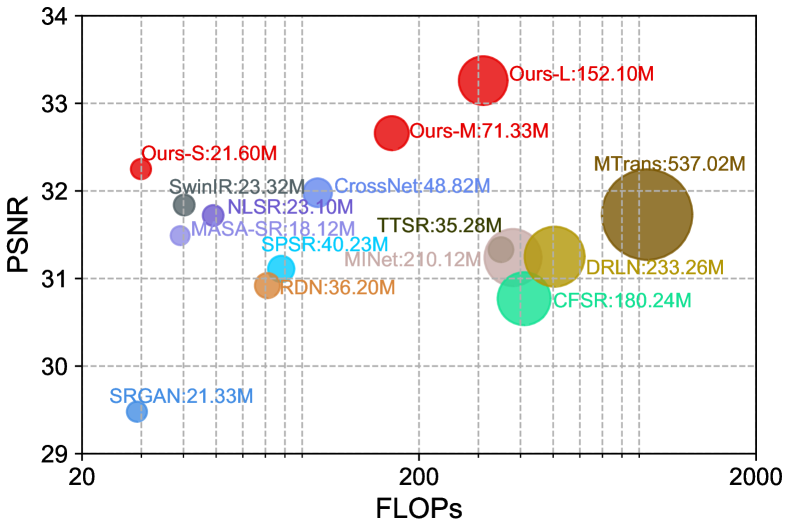
Quantitative Comparisons. On BraTS2018 dataset, our small variant ‘Our-S’ performs better than the best natural image super-resolution method SwinIR (Liang et al., 2021a) by 0.41dB, and the best reference-based image super-resolution method MASA-SR (Lu et al., 2021) by 0.81dB under the unsampling setting, while consuming fewer parameters and less memory cost (see Fig. 7). Compared to existing state-of-the-art MR image super-resolution method MTrans (Feng et al., 2021b), our final variant ‘Ours-L’ gives rise to PSNR gains of 4.2%, 3.3%, and 4.8% under , , and unsampling settings respectively. On IXI dataset, our method performs better than other methods as well. Particularly, it derives results with 3.1%, 3.5%, and 4.5% higher PSNR than the results of MTrans, under , , and upsampling settings, respectively.
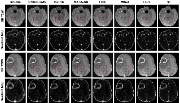
Qualitative Comparisons against other methods including SRResGAN (Umer et al., 2020), SwinIR (Liang et al., 2021a), TTSR (Yang et al., 2020), MASA-SR and MINet are presented in Fig. 6. Compared to images super-resolved by other methods, the results of our approach have more accurate local details. The gradient maps indicate that our method can generate HR T2WI with sharper and more complete structures.
Model Complexity. The model sizes and memory consumption of different methods are illustrated in Fig. 7. Overall, our method outperforms other super-resolution methods with fewer parameters and less memory cost.
4.4. Ablation Study
Extensive ablation studies are conducted on the BraTS2018 dataset under the upsampling setting to validate the efficacy of critical components in our method.
| Variant | PSNR | SSIM |
|---|---|---|
| baseline | 31.06 | 0.9225 |
| w/o S-IntraM-WA or L-IntraM-WA | 32.20 | 0.9306 |
| w/o S-IntraM-WA | 32.46 | 0.9362 |
| w/o L-IntraM-WA | 32.54 | 0.9380 |
| w/o InterM-A | 32.17 | 0.9345 |
| w/o InterH-Corr | 32.69 | 0.9406 |
| w/o AdaptIN | 32.77 | 0.9398 |
| full version | 33.26 | 0.9425 |
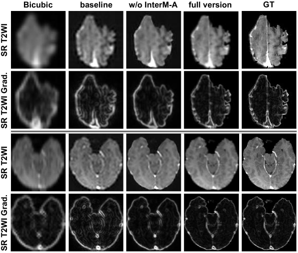
Efficacy of Attention Modules. We implement variants of our method by removing the attention modules or their inner units. The experimental results are reported in Table 2. The baseline model is formed by removing all intra-modality window attention and inter-modality attention modules. Without using the inter-modality attention (encoded as ‘w/o InterM-A’), the PSNR is dramatically decreased by 1.09dB compared to the full version of our method. Qualitative comparisons are provided in Fig. 9 to illustrate the efficacy of using inter-modality context information. As can be observed, after incorporating the gradient map of the T1WI with our devised inter-modality attention module, the structural information is recovered more completely. When both short-distance and long-distance intra-modality window attentions are abandoned (encoded as ‘w/o S-IntraM-WA or L-IntraM-WA’), the PSNR is decreased to 32.20dB, which is 1.06dB lower than that of the full version. Removing any separate short-distance (w/o S-IntraM-W) or long-distance (w/o L-IntraM-WA) window attention leads to performance degradation, which indicates that short-distance and long-distance dependencies have complementary effects in extracting the high-frequency structure priors. Without using the adaptive instance normalization (w/o AdaptIN) for aligning feature distributions across modalities, the PSNR is decreased by 0.49dB. The removing of the inter-head correlations (w/o InterH-Cor) in the basic attention module induces to 0.57dB PSNR reduction.
| Domain | Arch. | #Params | PSNR | SSIM |
|---|---|---|---|---|
| Input | CNN-RB | 171.127M | 31.86 | 0.9377 |
| Input | Cohf-T | 152.106M | 33.10 | 0.9409 |
| Gradient | CNN-RB | 171.127M | 31.90 | 0.9383 |
| Gradient | Cohf-T | 152.106M | 33.26 | 0.9425 |
Different Designs for Domain Prior Embedding. We apply different designs for exploring high-frequency structure priors and inter-modality context priors as in Table 3. We try to replace the Cofh-T with CNN-based residual blocks to capture intra-modality and inter-modality dependencies. Though more parameters are used, CNN-based residual blocks perform worse than Cofh-T (e.g., having 1.36dB lower PSNR under the gradient domain). It is also validated that the original input domain is sub-optimal to the exploration of domain prior information. Performing domain prior embedding in the original input domain produces results with 0.16dB lower PSNR than the gradient domain when Cofh-T is used for attention modeling.
| Metric | w/o | w/o SSIM Loss | Final Loss |
|---|---|---|---|
| PSNR | 32.33 | 32.86 | 33.26 |
| SSIM | 0.9410 | 0.9377 | 0.9425 |
Efficacy of Loss Components. According to the results in Table 4, the gradient level loss can improve the PSNR value while preserving the SSIM value. The SSIM loss is adopted for measuring the dissimilarity between local structures of predicted and ground-truth images. It can bring marginal gains to the SSIM value.
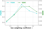
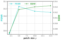
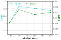
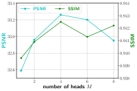
Choice of Hyper-parameters. The impact of hyper-parameters on the performance of our method is demonstrated in Fig. 8, from which we can observe that: 1) Our method achieves the best performance when the loss weighting coefficient is set to around 0.5; 2) For the inter-modality attention module, using too small patch size would be unfavorable to constructing reliable cross-modality dependencies, while the performance tends to be saturated after reaches 5; 3) For intra-modality window attention modules, larger window size would benefit to a more thorough exploration of relational structure priors. However, the performance saturates when becomes larger than 5; 4) Adopting more attention heads helps extract diversified types of relations. The performance increase as the grows within 4 and tends to be saturated when .
5. Conclusion
In this paper, we devise a novel Transformer-based framework to tackle the MR image super-resolution task. A Cross-modality high-frequency Transformer (Cohf-T) module is proposed for exploring structure priors from the gradient domain and inter-modality context from an additional modality. We extract intra-modality and inter-modality dependencies to capture the domain priors via the Transformer module. The inter-head correlations can bring extra promotion to feature enhancement in attention modules. The distribution alignment strategy based on adaptive instance normalization is beneficial for fusing features of different modalities. Experiments on two datasets demonstrate that our method achieves state-of-the-art performance on the MR image super-resolution task.
ACKNOWLEDGMENTS
This work was supported in part by the National Natural Science Foundation of China (No. 62003256, 62106235, 61876140, 62027813, U1801265, and U21B2048), in part by Open Research Projects of Zhejiang Lab (No. 2019kD0AD01/010), and in part by the Exploratory Research Project under Grant 2022PG0AN01.
References
- (1)
- Buades et al. (2011) Antoni Buades, Bartomeu Coll, and Jean-Michel Morel. 2011. Non-local means denoising. Image Processing On Line 1 (2011), 208–212.
- Chen et al. (2021b) Hanting Chen, Yunhe Wang, Tianyu Guo, Chang Xu, Yiping Deng, Zhenhua Liu, Siwei Ma, Chunjing Xu, Chao Xu, and Wen Gao. 2021b. Pre-trained image processing transformer. In CVPR.
- Chen et al. (2021a) Jieneng Chen, Yongyi Lu, Qihang Yu, Xiangde Luo, Ehsan Adeli, Yan Wang, Le Lu, Alan L Yuille, and Yuyin Zhou. 2021a. Transunet: Transformers make strong encoders for medical image segmentation. arXiv:2102.04306 (2021).
- Chen et al. (2018) Yuhua Chen, Yibin Xie, Zhengwei Zhou, Feng Shi, Anthony G Christodoulou, and Debiao Li. 2018. Brain MRI super resolution using 3D deep densely connected neural networks. In Proceedings of IEEE International Symposium on Biomedical Imaging.
- Cherukuri et al. (2019) Venkateswararao Cherukuri, Tiantong Guo, Steven J Schiff, and Vishal Monga. 2019. Deep MR brain image super-resolution using spatio-structural priors. IEEE TIP 29 (2019), 1368–1383.
- Dai et al. (2019) Tao Dai, Jianrui Cai, Yongbing Zhang, Shu-Tao Xia, and Lei Zhang. 2019. Second-order attention network for single image super-resolution. In CVPR.
- Dong et al. (2015) Chao Dong, Chen Change Loy, Kaiming He, and Xiaoou Tang. 2015. Image super-resolution using deep convolutional networks. IEEE TPAMI 38, 2 (2015), 295–307.
- Dosovitskiy et al. (2020) Alexey Dosovitskiy, Lucas Beyer, Alexander Kolesnikov, Dirk Weissenborn, Xiaohua Zhai, Thomas Unterthiner, Mostafa Dehghani, Matthias Minderer, Georg Heigold, Sylvain Gelly, et al. 2020. An image is worth 16x16 words: Transformers for image recognition at scale. arXiv:2010.11929 (2020).
- Fang et al. (2019) Chaowei Fang, Guanbin Li, Xiaoguang Han, and Yizhou Yu. 2019. Self-enhanced convolutional network for facial video hallucination. IEEE TIP 29 (2019), 3078–3090.
- Fang et al. (2022) Chaowei Fang, Liang Wang, Dingwen Zhang, Jun Xu, Yixuan Yuan, and Junwei Han. 2022. Incremental Cross-view Mutual Distillation for Self-supervised Medical CT Synthesis. In CVPR. 20677–20686.
- Feng et al. (2021a) Chun-Mei Feng, Huazhu Fu, Shuhao Yuan, and Yong Xu. 2021a. Multi-Contrast MRI Super-Resolution via a Multi-Stage Integration Network. arXiv:2105.08949 (2021).
- Feng et al. (2021b) Chun-Mei Feng, Yunlu Yan, Geng Chen, Huazhu Fu, Yong Xu, and Ling Shao. 2021b. MTrans: Multi-Modal Transformer for Accelerated MR Imaging. arXiv:2106.14248 (2021).
- Feng et al. (2021c) Chun-Mei Feng, Yunlu Yan, Huazhu Fu, Li Chen, and Yong Xu. 2021c. Task Transformer Network for Joint MRI Reconstruction and Super-Resolution. arXiv:2106.06742 (2021).
- Hendrycks and Gimpel (2016) Dan Hendrycks and Kevin Gimpel. 2016. Gaussian error linear units (gelus). arXiv:1606.08415 (2016).
- Huang and Belongie (2017) Xun Huang and Serge Belongie. 2017. Arbitrary style transfer in real-time with adaptive instance normalization. In ICCV.
- Iqbal et al. (2019) Zohaib Iqbal, Dan Nguyen, Gilbert Hangel, Stanislav Motyka, Wolfgang Bogner, and Steve Jiang. 2019. Super-resolution 1h magnetic resonance spectroscopic imaging utilizing deep learning. Frontiers in oncology 9 (2019), 1010.
- Jain et al. (2017) Saurabh Jain, Diana M. Sima, Faezeh Sanaei Nezhad, Gilbert Hangel, Wolfgang Bogner, Stephen Williams, Sabine Van Huffel, Frederik Maes, and Dirk Smeets. 2017. Patch-Based Super-Resolution of MR Spectroscopic Images: Application to Multiple Sclerosis. Frontiers in Neuroscience 11 (2017), 13.
- Ledig et al. (2017) Christian Ledig, Lucas Theis, Ferenc Huszár, Jose Caballero, Andrew Cunningham, Alejandro Acosta, Andrew Aitken, Alykhan Tejani, Johannes Totz, Zehan Wang, et al. 2017. Photo-realistic single image super-resolution using a generative adversarial network. In CVPR.
- Lee et al. (2019) Matthew CH Lee, Ozan Oktay, Andreas Schuh, Michiel Schaap, and Ben Glocker. 2019. Image-and-spatial transformer networks for structure-guided image registration. In International Conference on Medical Image Computing and Computer-Assisted Intervention.
- Liang et al. (2021a) Jingyun Liang, Jiezhang Cao, Guolei Sun, Kai Zhang, Luc Van Gool, and Radu Timofte. 2021a. SwinIR: Image restoration using swin transformer. In ICCV.
- Liang et al. (2021b) Tengfei Liang, Yi Jin, Yajun Gao, Wu Liu, Songhe Feng, Tao Wang, and Yidong Li. 2021b. CMTR: Cross-modality Transformer for Visible-infrared Person Re-identification. arXiv:2110.08994 (2021).
- Liu et al. (2018) Ding Liu, Bihan Wen, Yuchen Fan, Chen Change Loy, and Thomas S Huang. 2018. Non-local recurrent network for image restoration. arXiv:1806.02919 (2018).
- Liu et al. (2021) Ze Liu, Yutong Lin, Yue Cao, Han Hu, Yixuan Wei, Zheng Zhang, Stephen Lin, and Baining Guo. 2021. Swin transformer: Hierarchical vision transformer using shifted windows. arXiv:2103.14030 (2021).
- Lu et al. (2021) Liying Lu, Wenbo Li, Xin Tao, Jiangbo Lu, and Jiaya Jia. 2021. MASA-SR: Matching Acceleration and Spatial Adaptation for Reference-Based Image Super-Resolution. In CVPR.
- Ma et al. (2020) Cheng Ma, Yongming Rao, Yean Cheng, Ce Chen, Jiwen Lu, and Jie Zhou. 2020. Structure-preserving super resolution with gradient guidance. In CVPR.
- Mei et al. (2021) Yiqun Mei, Yuchen Fan, and Yuqian Zhou. 2021. Image Super-Resolution With Non-Local Sparse Attention. In CVPR.
- Menze et al. (2014) Bjoern H Menze, Andras Jakab, Stefan Bauer, Jayashree Kalpathy-Cramer, Keyvan Farahani, Justin Kirby, Yuliya Burren, Nicole Porz, Johannes Slotboom, Roland Wiest, et al. 2014. The multimodal brain tumor image segmentation benchmark (BRATS). IEEE Transactions on Medical Imaging 34, 10 (2014), 1993–2024.
- Niu et al. (2020) Ben Niu, Weilei Wen, Wenqi Ren, Xiangde Zhang, Lianping Yang, Shuzhen Wang, Kaihao Zhang, Xiaochun Cao, and Haifeng Shen. 2020. Single image super-resolution via a holistic attention network. In ECCV.
- Peng et al. (2021) Zhiliang Peng, Wei Huang, Shanzhi Gu, Lingxi Xie, Yaowei Wang, Jianbin Jiao, and Qixiang Ye. 2021. Conformer: Local Features Coupling Global Representations for Visual Recognition. arXiv:2105.03889 (2021).
- Pham et al. (2017) Chi-Hieu Pham, Aurélien Ducournau, Ronan Fablet, and François Rousseau. 2017. Brain MRI super-resolution using deep 3D convolutional networks. In Proceedings of IEEE International Symposium on Biomedical Imaging.
- Plenge et al. (2012) Esben Plenge, Dirk HJ Poot, Monique Bernsen, Gyula Kotek, Gavin Houston, Piotr Wielopolski, Louise van der Weerd, Wiro J Niessen, and Erik Meijering. 2012. Super-resolution methods in MRI: can they improve the trade-off between resolution, signal-to-noise ratio, and acquisition time? Magnetic Resonance in Medicine 68, 6 (2012), 1983–1993.
- Qingyun et al. (2021) Fang Qingyun, Han Dapeng, and Wang Zhaokui. 2021. Cross-Modality Fusion Transformer for Multispectral Object Detection. arXiv:2111.00273 (2021).
- Rousseau et al. (2010) François Rousseau, Alzheimer’s Disease Neuroimaging Initiative, et al. 2010. A non-local approach for image super-resolution using intermodality priors. Medical Image Analysis 14, 4 (2010), 594–605.
- Strudel et al. (2021) Robin Strudel, Ricardo Garcia, Ivan Laptev, and Cordelia Schmid. 2021. Segmenter: Transformer for Semantic Segmentation. arXiv:2105.05633 (2021).
- Tian et al. (2020) Chunwei Tian, Yong Xu, Wangmeng Zuo, Bob Zhang, Lunke Fei, and Chia-Wen Lin. 2020. Coarse-to-fine CNN for image super-resolution. IEEE Transactions on Multimedia 23 (2020), 1489–1502.
- Umer et al. (2020) Rao Muhammad Umer, Gian Luca Foresti, and Christian Micheloni. 2020. Deep generative adversarial residual convolutional networks for real-world super-resolution. In CVPRW.
- Vaswani et al. (2017) Ashish Vaswani, Noam Shazeer, Niki Parmar, Jakob Uszkoreit, Llion Jones, Aidan N Gomez, Łukasz Kaiser, and Illia Polosukhin. 2017. Attention is all you need. In NeurIPS.
- Wang et al. (2021) Longguang Wang, Xiaoyu Dong, Yingqian Wang, Xinyi Ying, Zaiping Lin, Wei An, and Yulan Guo. 2021. Exploring Sparsity in Image Super-Resolution for Efficient Inference. In CVPR.
- Wang et al. (2018) Xintao Wang, Ke Yu, Shixiang Wu, Jinjin Gu, Yihao Liu, Chao Dong, Yu Qiao, and Chen Change Loy. 2018. Esrgan: Enhanced super-resolution generative adversarial networks. In ECCVW.
- Yang et al. (2020) Fuzhi Yang, Huan Yang, Jianlong Fu, Hongtao Lu, and Baining Guo. 2020. Learning texture transformer network for image super-resolution. In CVPR.
- Yang et al. (2021) Junwei Yang, Xiao-Xin Li, Feihong Liu, Dong Nie, Pietro Lio, Haikun Qi, and Dinggang Shen. 2021. Fast T2w/FLAIR MRI Acquisition by Optimal Sampling of Information Complementary to Pre-acquired T1w MRI. arXiv:2111.06400 [eess.IV]
- Zhang et al. (2020) Dingwen Zhang, Guohai Huang, Qiang Zhang, Jungong Han, Junwei Han, Yizhou Wang, and Yizhou Yu. 2020. Exploring task structure for brain tumor segmentation from multi-modality MR images. IEEE TIP 29 (2020), 9032–9043.
- Zhang et al. (2021) Dingwen Zhang, Guohai Huang, Qiang Zhang, Jungong Han, Junwei Han, and Yizhou Yu. 2021. Cross-modality deep feature learning for brain tumor segmentation. PR 110 (2021), 107562.
- Zhang et al. (2018a) Yulun Zhang, Kunpeng Li, Kai Li, Lichen Wang, Bineng Zhong, and Yun Fu. 2018a. Image super-resolution using very deep residual channel attention networks. In ECCV.
- Zhang et al. (2018b) Yulun Zhang, Yapeng Tian, Yu Kong, Bineng Zhong, and Yun Fu. 2018b. Residual dense network for image super-resolution. In CVPR.
- Zhao et al. (2019) Xiaole Zhao, Yulun Zhang, Tao Zhang, and Xueming Zou. 2019. Channel splitting network for single MR image super-resolution. IEEE TIP 28, 11 (2019), 5649–5662.
- Zhu et al. (2020) Feida Zhu, Chaowei Fang, and Kai-Kuang Ma. 2020. Pnen: Pyramid non-local enhanced networks. IEEE TIP 29 (2020), 8831–8841.