Better Integrators for Functional Renormalization Group Calculations

Abstract

We analyze a variety of integration schemes for the momentum space functional renormalization group calculation with the goal of finding an optimized scheme. Using the square lattice $t-t^{\prime}$ Hubbard model as a testbed we define and benchmark the quality. Most notably we define an error estimate of the solution for the ordinary differential equation circumventing the issues introduced by the divergences at the end of the FRG flow. Using this measure to control for accuracy we find a threefold reduction in number of required integration steps achievable by choice of integrator. We herewith publish a set of recommended choices for the functional renormalization group, shown to decrease the computational cost for FRG calculations and representing a valuable basis for further investigations.

1 Introduction

The functional renormalization group (FRG) has proven itself to be a versatile theoretical framework to study competing ordering tendencies and other many-body phenomena both in itinerant fermionic salmhofer_honerkamp_2001_theory ; metzner_salmhofer_honerkamp_2012 ; platt_hanke_thomale_2013 and quantum spin systems ReutherOrig ; reuther2014cluster ; Iqbal3D ; BuessenDiamond ; PyrochlorePRX . The underlying flow equations are a large system of coupled, non-linear ordinary differential equations (ODEs), the solution of which stipulated the development of highly sophisticated numerical codebases tagliavini-ea-2019-multiloop ; Buessen2021 ; kiese2020multiloop . So far, algorithmical improvements mainly focussed on the efficient representation of vertex functions and optimizing momentum integrations on the right-hand-side (RHS) of the flow equations, with the numerical solution of the ODE itself only treated as a neccessity rather than an opportunity for improvements. Consequently, a simple Euler step was used in the majority of FRG calculations to date, see e.g. platt_hanke_thomale_2013 ; ReutherOrig ; Buessen2021 , with the inception of higher-order solvers from the Runge-Kutta family being a fairly recent development in the field kiese2020multiloop ; thoenniss2020multiloop ; bonetti2021single ; Markhof_2018 ; Weidinger_2017 ; PhysRevB.89.045128 ; Hauck_2021 .

The appropriate choice of integrator will lead to improved accuracy at the same number of evaluations of the RHS, which constitutes the main computational bottleneck of any FRG calculation. Alternatively, one can significantly reduce this number while maintaining good accuracy. In contrast to many other optimizations, this gain does not introduce any further physical approximations, but solely rests in mathematics. As a prototypical setup to study the influence of different integrators, we choose the momentum space FRG in the simplest truncation scheme, only considering the four-particle vertex $\Gamma^{(4)}$ while neglecting self-energy effects. Additionally, we limit ourselves to the well-understood case of the square lattice Hubbard model with hopping up to second nearest neighbors honerkamp-salmhofer-2001 ; honerkamp_doping_2001 ; honerkamp_salmhofer_furukawa_rice ; honerkamp2003 ; honerkamp_interaction_2004 ; honerkamp_ferromagnetism_2004 ; salmhofer_renormalization_2004 ; husesalm ; Uebelacker-2021-sffeedback ; husemann_frequency_2012 ; LichtensteinPHD ; tagliavini-ea-2019-multiloop ; hille-ea-2020-quantitative ; hille_pseudogap_2020 ; bonetti2021single ; schaefer-wentzell-multi-2021 .

We explicitly refrain from implementing more sophisticated approximation schemes vilardi2017nonseparable ; hille-ea-2020-quantitative ; tagliavini-ea-2019-multiloop ; reckling-honerkamp-2018 ; Uebelacker-2021-sffeedback ; bonetti2021single or multi-band extensions thomale2009functional ; kiesel-thomale-ea-2012 ; wang-frg-graphene-2012 ; platt_hanke_thomale_2013 ; lichtenstein-boeri-ea-2014 ; klebl2021moire , not only for clarity of analysis, but rather focus on benchmarking a large variety of different standard ODE solvers, most available in existing libraries rackauckas2017differentialequations ; boost_odeint . Nevertheless we expect our conclusions to provide a starting ground for the application of better integrators to more sophisticated physical approximations.

The paper is organized as follows: After an introduction of our notation of momentum space FRG and the approximations employed in our implementation in Section 2.1, we provide an overview over various integration schemes in Section 2.2 and define tangible metrics to judge the quality of the different schemes in Section 2.3. In Section 3 we employ a two-stage elimination procedure. In a first step we sort out all integrators incapable of reproducing the physical ordering instability for the nearest-neighbor only model. We subsequently analyze the remaining set over a larger parameter space including second-neighbor hopping to distinguish optimal choices.

2 Methods

2.1 FRG in brevity

The following discussion of FRG will be reduced to an absolute minimum and only serves as a means to introduce the notation used. For detailed derivations we refer the interested reader to standard literature salmhofer_honerkamp_2001_theory ; metzner_salmhofer_honerkamp_2012 ; platt_hanke_thomale_2013 .

In the following, we will focus solely on the square-lattice $t-t^{\prime}$ Hubbard model defined by

$$\begin{split}H_{0}=&-\!\sum\limits_{\braket{i,j},\sigma}t\,c_{i,\sigma}^{\dagger}c_{j,\sigma}^{\phantom{\dagger}}\,-\!\sum_{\braket{\braket{i,j}},\sigma}t^{\prime}\,c_{i,\sigma}^{\dagger}c_{j,\sigma}^{\phantom{\dagger}}\\ &-\!\sum_{i,\sigma}\mu\,c_{i,\sigma}^{\dagger}c_{i,\sigma}^{\phantom{\dagger}}\,,\end{split}$$ (1)

$$H_{\mathrm{I}}= U\,\sum_{i,\sigma}\,n_{i,\sigma}n_{i,\bar{\sigma}}\,,$$ (2)

where $t$ ($t^{\prime}$) denote (next-) nearest-neighbor hopping amplitudes, $\mu$ is the chemical potential and $U$ the strength of the onsite Hubbard interaction. Due to the spin-rotation invariance of Eq. 1 and Eq. 2, we can constrain our derivation to the $\operatorname{SU}(2)$-symmetric set of equations. To simplify the functional dependence of the FRG equations, we invoke the static approximation of the problem, i.e. consider only the zero Matsubara frequency component of the vertex functions, and neglect self-energy effects honerkamp2003 ; platt_hanke_thomale_2013 .

The $\operatorname{SU}(2)$-reduced FRG equation in the conventional truncation scheme including contributions up to the four-point vertex $\Gamma^{(4)}$ is diagrammatically shown in Fig. 1 and can be expanded to (using $V$ as $\operatorname{SU}(2)$-symmetrized four-point vertex):

$$\frac{\mathrm{d}}{\mathrm{d}\Lambda} V_{\boldsymbol{k}_{0},\boldsymbol{k}_{1},\boldsymbol{k}_{2}}=$$

$$\phantom{+}\,\,\,V_{\boldsymbol{k}_{0},\boldsymbol{k}_{1},\boldsymbol{l}}\dot{L}^{-,\Lambda}_{\boldsymbol{l},-\boldsymbol{l}+\boldsymbol{k}_{0}+\boldsymbol{k}_{1}}V_{\boldsymbol{l},-\boldsymbol{l}+\boldsymbol{k}_{0}+\boldsymbol{k}_{1},\boldsymbol{k}_{2}}$$

$$+V_{\boldsymbol{k}_{0},\boldsymbol{l}-\boldsymbol{k}_{0}+\boldsymbol{k}_{2},\boldsymbol{k}_{2}}\dot{L}^{+,\Lambda}_{\boldsymbol{l},\boldsymbol{l}-\boldsymbol{k}_{0}+\boldsymbol{k}_{2}}V_{\boldsymbol{l},\boldsymbol{k}_{1},\boldsymbol{l}-\boldsymbol{k}_{0}+\boldsymbol{k}_{2}}$$

$$+V_{\boldsymbol{k}_{0},\boldsymbol{l}-\boldsymbol{k}_{0}+\boldsymbol{k}_{2},\boldsymbol{k}_{2}}\dot{L}^{+,\Lambda}_{\boldsymbol{l},\boldsymbol{l}-\boldsymbol{k}_{0}+\boldsymbol{k}_{2}}V_{\boldsymbol{k}_{1},\boldsymbol{l},\boldsymbol{l}-\boldsymbol{k}_{0}+\boldsymbol{k}_{2}}$$ (3)

$$+V_{\boldsymbol{k}_{0},\boldsymbol{l}-\boldsymbol{k}_{0}+\boldsymbol{k}_{2},\boldsymbol{l}}\dot{L}^{+,\Lambda}_{\boldsymbol{l},\boldsymbol{l}-\boldsymbol{k}_{0}+\boldsymbol{k}_{2}}V_{\boldsymbol{l},\boldsymbol{k}_{1},\boldsymbol{l}-\boldsymbol{k}_{0}+\boldsymbol{k}_{2}}$$

$$+V_{\boldsymbol{k}_{0},\boldsymbol{l}-\boldsymbol{k}_{1}+\boldsymbol{k}_{2},\boldsymbol{l}}\dot{L}^{+,\Lambda}_{\boldsymbol{l},\boldsymbol{l}+\boldsymbol{k}_{1}-\boldsymbol{k}_{2}}V_{\boldsymbol{l},\boldsymbol{k}_{1},\boldsymbol{k}_{2}}\,,$$

where we suppress the, in the $\operatorname{SU}(2)$ Hubbard model, unnecessary spin indices. We also use a modified Einstein sum convention to indicate the momentum-integration in $\boldsymbol{l}$ over the Brillouin zone (BZ). To treat the continuous momentum-dependence of the vertex function, we employ the “grid-FRG” momentum discretization scheme in the BZ with the additional refinement-scheme described in Ref. beyer_hauck_klebl . Eq. 3 will commonly be referred to as the right-hand side (RHS) of the FRG equation, which we need to compute at each flow step iteration.

The $\dot{L}^{\Lambda}$ given in the RHS equation is the derivative w.r.t. the scale $\Lambda$ of the regulated loop

$$L^{\pm,\Lambda}=\sum\limits_{n}G^{\Lambda}(\boldsymbol{k},\mathrm{i}\omega_{n})G^{\Lambda}(\boldsymbol{k}^{\prime},\pm\mathrm{i}\omega_{n})\,.$$ (4)

The FRG regulator $\Theta(\Lambda)$ here is introduced multiplicatively by defining $G^{\Lambda}=\Theta(\Lambda)G$ where $G$ is the bare propagator. We have used both the particle-particle loop $L^{-,\Lambda}$ and the particle-hole loop $L^{+,\Lambda}$ in out notation. As a regulator we choose the $\Omega$-cutoff $\Theta(\Lambda)=\frac{\omega^{2}}{\omega^{2}-\Lambda^{2}}$ husesalm with high numerical stability. The analytic Matsubara frequency summations then yield:

$$\dot{L}^{\pm,\Lambda}_{\boldsymbol{l},\boldsymbol{l}^{\prime}} =\frac{\mathrm{d}}{\mathrm{d}\Lambda}L^{\pm,\Lambda}_{\boldsymbol{l},\boldsymbol{l}^{\prime}}$$ (5)

$$=\begin{cases}\displaystyle\frac{\pm 1/4}{\epsilon\mp\epsilon^{\prime}}\left(\frac{\epsilon(3\lvert\epsilon\rvert+\Lambda)}{(\lvert\epsilon\rvert+\Lambda)^{3}}\mp\frac{\epsilon^{\prime}(3\lvert\epsilon^{\prime}\rvert+\Lambda)}{(\lvert\epsilon^{\prime}\rvert+\Lambda)^{3}}\right)\\[10.00002pt] \displaystyle\mp\frac{3\epsilon^{2}-4\lvert\epsilon\rvert\Lambda-\Lambda^{2}}{4(\lvert\epsilon\rvert+\Lambda)^{4}}\qquad\text{if }\epsilon=\epsilon^{\prime}\ .\end{cases}$$ (6)

To obtain the effective low-energy vertex we integrate the differential equation (RHS) starting at infinite (i.e. large compared to bandwidth) $\Lambda=\Lambda_{\infty}$ and approach $\Lambda\rightarrow 0$. When encountering a phase transition the loop derivatives will diverge in conjunction with the associated susceptibilities and we terminate the flow. This is the integration for which we attempt to find an optimized solver. Due to the divergence we can not finalize the calculations using the solvers but instead hard-terminate them once the maximum element of the vertex exceeds a threshold $V_{\max}$.

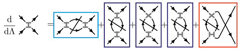
Figure 1: Diagrammatic representation of the functional renormalization group equations. We show the $\operatorname{SU}(2)$-symmetric flow equation, where the $\operatorname{SU}(2)$-degree of freedom is kept constant along the lines of the vertex. The line through the loop represents the scale derivative $\mathrm{d}/\mathrm{d}\Lambda$. We have indicated the three channels of the FRG flow, differing in the bosonic transfer momentum: $P$-, $C$-, and $D$-channel.

2.2 Integrators

The possible choices of integrators are plentiful but in the following we highlight some of the most prevalent algorithms as well as some which will prove to excel during our testing. The measurement schemes used to determine quality are provided at the end of this section. In order to numerically solve the non-linear non-autonomous differential equation

$$\frac{\mathrm{d}}{\mathrm{d}\Lambda}V=\mathrm{RHS}(V,\Lambda)$$ (7)

we utilize both single-step and multi-step methods Hairer2008 in order to obtain an iteration procedure

$$V_{n+1}=V_{n}+\Delta_{\Lambda,n}\Phi(\Lambda_{n},V_{n},\Delta_{\Lambda,n})$$ (8)

that we terminate at the divergence of $V$.

We almost exclusively focus on integrators that are implemented in the excellent DifferentialEquations.jl package rackauckas2017differentialequations written in the Julia programming language. We emphasize integrators that are well-known and commonly employed, such as the Runge-Kutta class and also widely available in other programming languages. A full list of the considered (including all disregarded) integrators can be found in Appendix A.

2.2.1 Single-Step Methods

A single-step method is characterized by utilizing at each step a starting value $V_{n}$ and additional evaluations of the RHS to construct $V_{n+1}$. The most well-known family of methods in this class are the Runge-Kutta type integrators where the function $\Phi$ is constructed as a weighted average of evaluations of RHS within the interval $[\Lambda_{n},\Lambda_{n+1}]$ such that it coincides up to the respective order with its Taylor polynomial:

$$V_{n+1}=V_{n}+\Delta_{\Lambda}\sum_{i=1}^{s}b_{i}k_{i}$$ (9)

$$k_{i}=\mathrm{RHS}(\Lambda_{n}+c_{i}\Delta_{\Lambda},V_{n}+\Delta_{\Lambda}\sum_{j=1}^{s}a_{ij}k_{j})$$ (10)

The method is explicit if $a_{ij}=0$ for $j\geq i$ else it is an implicit method. Adaptivity can be included by a time-step dependent $\Delta_{\Lambda,n}$. The specifics of the methods are covered in tremendous detail in the literature, e.g., Hairer2008 .

2.2.2 Example: Adaptive Explicit Euler

The conceptually simplest integrator in FRG that serves as the baseline for this work is the adaptive explicit Euler described in Algorithm 1. Note that we have included a function $f(\Lambda,V_{\max})=\min(\max(a\Lambda/V_{\max},\Delta_{\min}),\Delta_{\max})$ which is an adaption scheme specifically designed to reduce the step-width in the proximity of the expected flow divergence. Here $a$ is a small number determining the relative speed of the integration.

Algorithm 1 Explicit adaptive Euler

1:$V=V_{0}$, $\Lambda=\Lambda_{0}$

2:while $\max(V)<V_{\max}$ and $\Lambda>0$ do

3:     $\mathrm{d}V=\mathrm{RHS}(V_{n},\Lambda)$

4:     $V_{n+1}=V_{n}+\Delta_{\Lambda}\mathrm{d}V$

5:     $\Lambda_{n+1}=\Lambda_{n}-\Delta_{\Lambda}$

6:     $\Delta_{\Lambda}=f(\Lambda,V_{\max})$

7:end while

2.2.3 A note on implicit Runge-Kutta methods

We have attempted to include implicit integration schemes in our analysis but were inhibited by their high memory cost. While for explicit methods the requirements are understood to be $n\times\texttt{sizeof}(V),n\in\mathbb{N}$, for the implicit methods we must instead consider the size of the Jacobian we are attempting to invert. This is proportional to the square of the size of a single solution (as it is a linear map between two of them) and is thus $\propto\texttt{sizeof}(V)^{2}$. Even for the relatively small scale systems we employ here the number of elements is $n_{\boldsymbol{k}}^{6}\approx 10^{13}$. All implicit integrators will therefore not be a viable option for FRG calculations.

2.2.4 Methods based on the Non-linear Magnus Series

Another class of one-step methods specifically suited for homogeneous, non-linear, non-autonomous ODEs is based on suitable approximations $\Omega^{[m+1]}$ of the Magnus operator $\Omega$ Casas2006 in the formal exact solution of (7),

$$V(\Lambda)=\exp\left(\Omega(\Lambda,V_{\infty})\right)V_{\infty}$$ (11)

where $V_{\infty}=V(\Lambda=\infty)$. For the following approximations we define the matrix $A$ by the relation $\mathrm{RHS}(\Lambda,V)=A(\Lambda,V)V$. In this overview of methods we restrict ourselves to the approximations of first,

$$\Omega^{[1]}(\Lambda,\Lambda_{\infty})=\int_{\Lambda_{\infty}}^{\Lambda}A(s,V_{\infty})ds$$ (12)

and second order

$$\Omega^{[2]}(\Lambda,\Lambda_{\infty})=\int_{\Lambda_{\infty}}^{\Lambda}A(s,e^{\Omega^{[1]}}V_{\infty})ds.$$ (13)

and refer the reader to the literature Casas2006 for expressions of the higher order in terms of iterated commutators.

An iterative procedure is obtained by applying the approximate time evolution operator $\exp(\Omega^{[m]})$ for small steps $\Delta_{\Lambda}$ such that

$$y_{n+1}=\exp(\Omega^{[m]})y_{n}.$$ (14)

Approximating the integrals in Eq. 12 and Eq. 13 by order-consistent low-order approximations, such that e.g., at first order

$$\Omega^{[1]}(\Lambda+\Delta_{\Lambda},\Lambda) =\int_{\Lambda}^{\Lambda+\Delta_{\Lambda}}A(s,V(\Lambda))ds$$

$$\approx\Delta_{\Lambda}A(\Lambda,V(\Lambda))ds.$$

Adaptivity is easily included by using time slices of differing times $\Delta_{\Lambda,n}$ determined by the same strategy as for the adaptive Euler.

2.2.5 Multistep/Adams methods

In contrast to one-step methods, multistep methods utilize previous evaluations of the right hand side, $f_{n+k}=\mathrm{RHS}(V_{n+k},\Lambda_{n+k})$ in order to approximate it with a Lagrange polynomial. The general form of these linear multistep methods can be stated as

$$\sum_{j=0}^{k}\alpha_{j}V_{n+j}=h\sum_{j=0}^{k}\beta_{j}\mathrm{RHS}(\Lambda_{n+j},V_{n+j}).$$ (15)

If $\beta_{k}=0$ the method is explicit and does not require the evaluation of RHS at unknown points. Commonly this class is termed Adams-Bashforth technique. Otherwise the method is implicit. If the interpolation polynomial is only augmented with the single yet unknown point $\mathrm{RHS}(\Lambda_{n+k},V_{n+k})$ the method is termed Adams-Moulton method. In this case the implicit nature can be treated by employing a predictor-corrector scheme where the prediction $\hat{V}$ is obtained by an explicit Adams method of one order lower than the implicit method, RHS is evaluated and the new value $V_{n+k}$ is obtained. Multistep methods need startup values, but these are obtained with explicit Runge-Kutta or similar methods. Adaptive step size integrators can be obtained by utilizing more sophisticated interpolation techniques.

2.3 Measures of Quality

Differentiation of the quality of integrators will be based on the following aspects:

1. Error compared to a converged high-fidelity Euler calculation

2. Minimal number of RHS-evaluations

3. RAM requirements

2.3.1 Error compared to high fidelity Euler

All integrators must converge to the same result at infinite numbers of steps performed, or equally at negligible integration error for adaptive procedures. To obtain this result in the most controlled fashion we converge an adaptive Euler integrator to a high number of steps ($N_{\mathrm{RHS}}\approx 6000$) as a reference. The measure of error employed in the comparison is the normed sum of differences in the resulting vertex tensor:

$$\frac{\sum_{i}\lvert V(i)-V_{\mathrm{Euler}}(i)\rvert}{\sum_{i}\lvert V_{\mathrm{Euler}}(i)\rvert}\,.$$ (16)

To avoid numerical discrepancies in the vicinity of the flow divergence, we instead compare the vertices slightly above the critical scale $\Lambda_{\mathrm{crit}}$ at $\Lambda=0.17$. This scale is sufficiently low for the integrator to have performed a significant number of integration steps but sufficiently high to avoid the critical scale. Note that this number is arbitrarily chosen to lie within this region.

Because this measure does not include an analysis of the error size which is tolerable for qualitatively correct FRG results (for the given approximation level), we have additionally in stage 2 Section 3.2 included a full phase scan to ensure the results are consistent with expected behavior. We eliminate all integrators that are inconsistent.

2.3.2 Minimal number of RHS-evaluation

As we are aiming to optimize the calculation time requirements, the most important measure of quality for any integration routine must be the number of RHS-evaluations it requires until divergence. This is the only expensive part of the calculation and is thus a trivial, but platform independent estimator for the runtime. While this is no longer true for implicit integrators where the inversion of the Jacobian would be most expensive, these are disallowed by their RAM requirements and thus can be neglected here.

2.3.3 Memory requirement

For most FRG calculations the bottleneck is not only the calculation time but also the memory consumption beyer_hauck_klebl ; lichtenstein_high-performance_2017 . As higher-order methods may require the saving of intermediate results we want to track the number of concurrently allocated vertex-sized objects as a measure of RAM usage. Once again for implicit methods this may not be the most accurate measure due to the creation of high-dimensional Jacobian matrices, but we disregard them entirely. The impact on memory usage by other objects is of second order when compared to the vertices in scaling: The vertices scale as $N_{\boldsymbol{k}}^{3}$ while the loop-derivatives scale as $N_{\boldsymbol{k}}^{2}$ and the dispersion cache scales as $N_{\boldsymbol{k}}N_{\boldsymbol{k}_{f}}$. The measure chosen is the peak memory usage during the calculations. This will be highly proportional to the total number of vertex objects though slight lower-order effects are to be expected.

3 Results

We have ensured that our implementation falls within the FRG equivalence class of the Hubbard model reported on in Ref. beyer_hauck_klebl . This binary equivalence is sufficient as a proof of correctness. Note that while one of the codes in that publication is written by one of us, we utilize for this benchmark an independent implementation written in the Julia programming language.

All simulations were performed using the following parameters: $t=1,U=3t,t^{\prime}\in[0.0,...,-0.5]t$, $\mu=-4t^{\prime}$. We use a momentum meshing of $n_{\boldsymbol{k}}=16\times 16$ with a refined meshing of $n_{\mathrm{fine}}=9\times 9$. The FRG flow is started at $\Lambda_{\infty}=50$ and tracked until the maximum element of the vertex exceeds $V_{\max}=50t$, where we terminate the integration and analyze the last vertex $V_{\Lambda_{\mathrm{crit}}}$ with respect to its ordering tendencies. While this resolution is insufficient for physical simulations at low scales and we acknowledge that the stability of all integrators increases for higher resolutions, the fact that most integrators calculate the proper results is testament to a sufficient resolution for this analysis.

We have split the investigation into a two staged elimination process where we iterate over consecutively more involved tests to find the best set of integrators and neglect the remainder.

3.1 Stage 1

The first approach to determine the feasibility of the integrators is to analyze the square lattice Hubbard model at $t^{\prime}=0$, $\mu=0$ where we expect antiferromagnetic ordering.

The results of stage 1 are displayed in Fig. 2. We now select the subset of integrators which yield a speedup (or are similar) in number of evaluations when compared to the adaptive Euler integration scheme while maintaining higher or similar accuracy. This reduces our list of integrators to consider for the continuation to be:

• Adaptive Euler

• Bogacki-Shampine 3/2 (BS3)

• Dormand-Prince’s 5/4 Runge-Kutta (DP5)

• Second order Heun’s

• Second order Midpoint

• canonical Runge-Kutta 4 (RK4)

• Strong-stability preserving Runge-Kutta (SSPRK43)

• Tsitouras 5/4 Runge-Kutta (Tsit5)

• Third order Adams-Moulton, BS3 for starting values (VCABM3)

• Tanaka-Yamashita 7 Runge-Kutta (TanYam7)

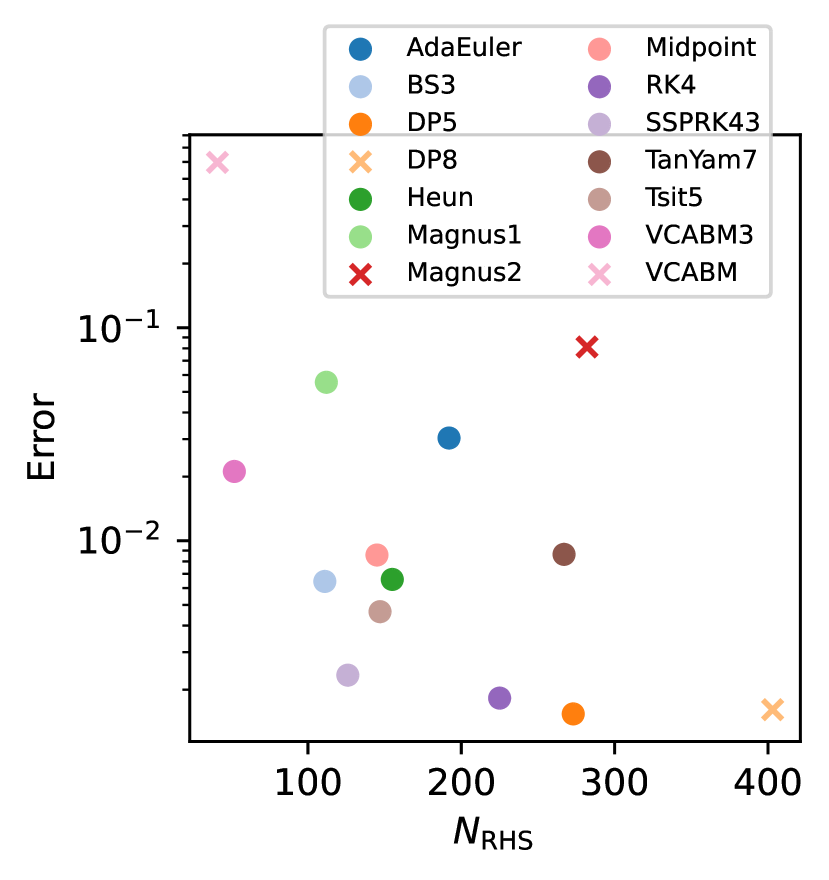
Figure 2: Integrator Comparisons Quick analysis of the quality of integrators. For this measurement we chose the single point at $t^{\prime}=0$, $\mu=0$ in the $t-t^{\prime}$ square-lattice Hubbard model. At this point we expect an antiferromagnetic divergence, every method incapable of producing this is omitted. We show the number of steps required by the integrators for the prediction of the divergence as well as the error when compared to high-fidelity Euler calculations. The best integrators lie near the origin of the coordinate system, low number of steps and negligible error. We in the following will consider only integrators within the marked region, the set of which we will refer to as stage 2 integrators. A full list of considered integrators as well as the reasons some are not shown can be found in Appendix A.

We have thus significantly reduced the number of integrators to consider in the next section. While we acknowledge that some of these might have been tweaked into compliance by optimizing parameters we insist on the out-of-the-box setup of the integrators being at least sufficient (if maybe not optimal).

3.2 Stage 2

To check the reduced set of integrators for physical consistency we now evaluate the $t-t^{\prime}$ square lattice Hubbard model at van Hove filling by scanning the second neighbor hopping $t^{\prime}$ (adapting the chemical potential $\mu=4t^{\prime}$ accordingly to remain at v.H. filling) as previously calculated in Refs. LichtensteinPHD ; salmhofer_honerkamp_2001_theory . We perform these calculations with each of the second stage integrators to obtain a more qualified understanding of their accuracy and cost.

To determine accuracy we in a first step check that the phase transitions occur in a controlled manner in all integrators and all points are properly found to diverge. In this we however make an exception near the SC-FM phase transitions, where the low integration resolutions used here will lead to uncontrolled behavior. By this process we eliminate the Midpoint and TanYam7 integration methods, which did not properly reproduce the leading instability for some points in the phase diagram. The remaining results and integrators are shown in Fig. 3/ We can here also see the good agreement of qualitative results from the different integrators, an expected but satisfying result.

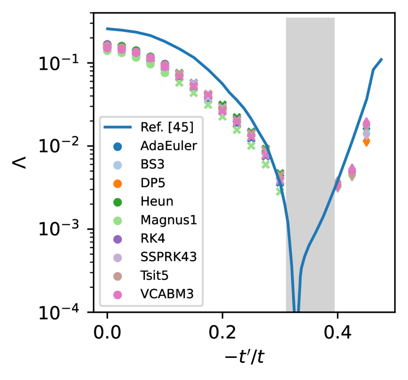
Figure 3: Hubbard Model Calculations of the reference Hubbard model at van Hove filling with $t^{\prime}\in[0.0,-0.4t]$. The comparative data is taken from Honerkamp_2001 , on which we have superimposed the subset of stage 2 integrators. We have removed all integrators who were unable to produce the correct phase at points. Note that we in this analysis ignore the region around the SC-FM phase transition as it is notoriously unstable under low scales LichtensteinPHD ; beyer_hauck_klebl . Dots represent antiferromagnetism, crosses superconductivity and diamonds ferromagnetism.

To evaluate the performance we sum the number of RHS evaluation for each of the 20 runs in the interval $t^{\prime}\in[0,...,-0.5]$ into a total number $N_{\mathrm{RHS}}$. This is a more accurate measure of performance than before as the phase diagram contains parameter regions, where early divergences are expected as well as points, at which low RG scales have to be reached. This is supplemented by an improved error estimate: As before we calculate the effective vertex at the low scale of $\Lambda=0.17$ and compare it to the results obtained by a converged high-fidelity Euler, but we now consider 3 additional points, one in each phase at $t^{\prime}=0.0,-0.05,-0.2,-0.45$. As an accuracy measure we consider the mean of the relative error for these four parameter combinations. The results of this analysis are presented in Fig. 4. We find, that depending on the exact requirements on the integrator, different algorithms should be employed. For purely optimizing the runtime, i.e. the number of RHS evaluations, the multi-step method VCABM3 clearly is the method of choice, with a mean error comparable to the adaptive Euler, but only needing less than a quarter of RHS evaluations. On the other extreme, we find DP5 to be the most accurate, but requiring 40% more runtime. A competitive alternative is RK4 with a slightly larger relative deviation from the reference data, but at a computational cost comparable to the Adaptive Euler. As a good compromise between numerical complexity and accuracy, we find a cluster of three methods: BS3, Tsit5 and, most notably, SSPRK43 all have an order of magnitude lower relative error, but at roughly two third of the computational cost of the Adaptive Euler.

In Fig. 5 we additionally show the measured peak memory requirement of our implementation relative to the Adaptive Euler. This figure is highly implementation dependent, but should nevertheless serve as a rough guide to the overhead incurred by the different solvers. Most clearly, this figure shows, that the extreme numerical efficiency of VCABM3 is achieved trading runtime for memory consumption, with a fivefold requirement compared to a simple Euler implementation. The remaining integrators considered all fall in the range of 1.5 to 2.5 the memory requirement. Out of the three general algorithms, SSPRK43 clearly has the lowest memory requirements, which combined with its good accuracy and numerical efficiency makes it the best suited ODE integrator in our benchmark, followed closely by BS3.

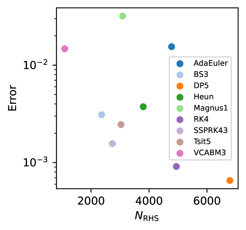
Figure 4: Stage 2 Integrator Comparisons We compare the integrators which passed the primary analysis in a second iteration using an extended testing scheme. This extended scheme consists of a full $t-t^{\prime}$ Hubbard model phase scan. The $N_{\mathrm{RHS}}$ here represents the total number of steps for the evaluation of the 20 points in the phase diagram. Similarly the error represents the mean of the errors at the four evaluation points $t^{\prime}=0,-0.05,-0.2,-0.4$. Once again proximity to the origin is the quality measure in the graphic.

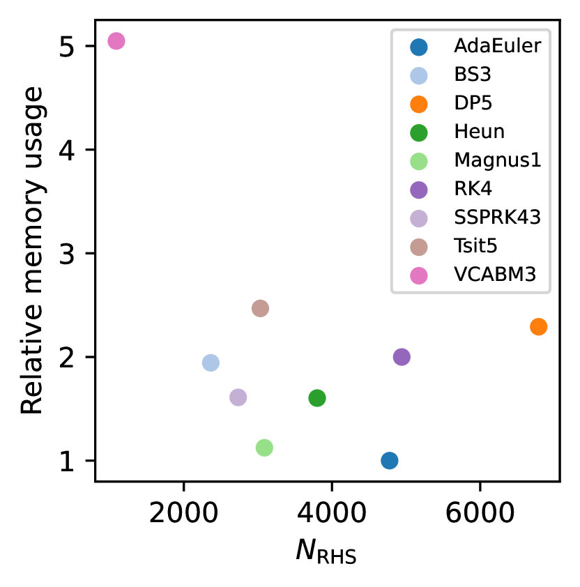
Figure 5: Stage 2 Memory Comparison Supplementing the analysis presented in Fig. 4 we here provide the measurements of the memory usage during the integration procedure. We have denoted the memory usage in terms of the most efficient schemes, the adaptive Euler. Note that we have just measured the total memory usage, partial might thus correspond to objects of smaller size. Nonetheless the measurement will reflect the ram needed for the integrations very well.

4 Conclusions

We have benchmarked a multitude of ODE integration algorithms both from the DifferentialEquations.jl library and own implementations against a reference Adaptive Euler using the square-lattice Hubbard model as a test case. We have identified, that the right choice of integrator can significantly reduce the numerical cost for integrating the runtime while at the same time producing more accurate results. We identify the multi-step algorithm VCABM3 to be the most efficient one with acceptable numerical errors, while highest accuracy can be achieved by the numerically expensive DP5 algorithm, or alternatively the slightly less accurate RK4, which however has about the same numerical cost as the Adaptive Euler.

As the best compromise between accuracy and numerical speedup, we identify Tsit5, BS3 and SSPRK43, with the latter slightly outclassing its rivals. This fact at first glance is surprising, as this specific integrator is designed to handle dissipative differential equations stemming from a discretization of hyperbolic partial differential equations. However, as the FRG equations are believed to flow towards a fixed point for any given phase, we speculate them to exhibit dissipation in the mathematical sense, which is the property SSPRK43 is design to utilize. This means that solutions of the RG flow corresponding to different initial conditions in the same phase become more similar as they approach $\Lambda=0$, as the dominant physics will be the same for all of these. A mathematically thorough analysis of the FRG equations regarding this property, however, is beyond the scope of this paper.

As we only have analyzed a subset of the plethora of available ODE integrators in this paper, we cannot claim to have found the “best” integrator for FRG system, but we ensured to represent a spectrum of the common choices.

We also have focused on the simplest physically interesting model, the square-lattice Hubbard model. While we believe, that the scaling of computational cost can be extrapolated to other problems, more complicated problems posed with more intricate Fermi surfaces may require denser integration steps, the best algorithms may therefore differ.

Furthermore when using other approximations of momentum space FRG, for example self energy inclusions or multiloop, the RHS equations are subject to structural changes. The inclusion of self energies might benefit from the use of operator splitting methods, such as the generalized Strang or Leapfrog splitting McLachlan1995 , where self energy and vertex are evaluated at alternating half-step intervals. The merit of our results is still valid, the best integrators as found here will be good candidates for the other applications.

Another path of algorithmic progress can be made by taking into account to intricacies of the FRG equations. Since their integration starts at infinity we propose to investigate transformations of this semi-infinite domain as in Ref. macdonald ; PhysRevB.89.045128 ; in_prep_hauck .

Furthermore, the integration of the FRG equations contains an inherent singularity corresponding to the physical ordering tendency. Implicit methods wanner1996 are well suited for such problems, but were out of the scope of our investigation due to memory requirements. It could be a worthwhile direction of future investigation. More specialized multistep integrators that utilize rational interpolants Karimov2021 ; wanner1996 instead of Newton and Lagrange polynomials for the definition of their integration rule could be beneficial in dealing with the singular behavior. But of course their effectiveness rests on methods of obtaining the action of the Jacobian of $RHS$ or suitable approximations to it.

Acknowledgments J.B.thanks GRF (German Research Foundatation) for support through RTG 1995 within the Priority Program SPP 244 “2DMP”. F.G. and T.M. thank the GRF for funding through the SFB 1170 “Tocotronics” under the grant numbers Z03 and B04, respectively. Furthermore we want to thank Jonas Hauck, Dominik Kiese, Lennart Klebl, Janik Potten, Stephan Rachel and Tilman Schwemmer for helpful discussions.

Author’s contributions J.B. and T.M. were leading the development of the code with F.G. taking charge of the simulation effort. Analysis was conducted on a joint basis, the manuscript was a joint effort by the authors. Overall no distinction can be drawn in level of contribution between the authors.

Data availability The FRG implementation used in this paper is available at https://doi.org/10.5281/zenodo.6391339. The numerical data shown is available from the corresponding author upon reasonable request.

Appendix A Full list of considered integrators

Name	Comment	Reason if discarded
AB3, AB5, ABM32, ABM54	Hairer2008	(Not adaptive)
Adaptive Euler	Hairer2008
Adaptive Magnus1	Casas2006
Adaptive Magnus2	Casas2006	(Error S1)
BS3	Bogacki1989
CVODE	rackauckas2017differentialequations	(complex arithmetic)
DP5	Dormand1980
DP8 (Runtime S1)	Hairer2008
EPIRK4s3A	rackauckas2017differentialequations	(not adaptive)
exp4	rackauckas2017differentialequations	(not adaptive)
exprb32	rackauckas2017differentialequations
Feagin10 (Wrong S1)	feagin2012high	(issues calculating jacobian)
FRK65	rackauckas2017differentialequations	(very excessive runtime)
Heun	Hairer2008
HochOst4	rackauckas2017differentialequations	(not adaptive)
implicit Euler	wanner1996	(Memory)
implicit Midpoint	wanner1996	(Memory)
KenCarp4	rackauckas2017differentialequations	(Memory)
Kvaerno5	rackauckas2017differentialequations	(Memory)
LawsonEuler	rackauckas2017differentialequations	(Memory)
Midpoint	Hairer2008	(Wrong Hubbard)
NorsettEuler	rackauckas2017differentialequations	(Not adaptive)
QBD, QNDF, QBDF1, QNDF1	rackauckas2017differentialequations	(Memory)
RadauIIa3, RadauIIa5	rackauckas2017differentialequations	(complex arithmetic)
RK4	Hairer2008
RKO65	rackauckas2017differentialequations	(Not adaptive)
ROCK2, ROCK4	rackauckas2017differentialequations	(excessive runtime)
Rodas4p2	rackauckas2017differentialequations	(Memory)
Ros3p	rackauckas2017differentialequations	(Memory)
Rosenbrock23	rackauckas2017differentialequations	(Memory)
SDIRK	rackauckas2017differentialequations	(Memory)
SSPRK22, SSPRK33, SSPRK83	rackauckas2017differentialequations	(Not adaptive)
SSPRK43	Kraaijevanger_1991
SSPRK932	rackauckas2017differentialequations	(type errors, excessive runtime)
TanYam7	tanaka1992	(Wrong Hubbard)
Trapezoid	wanner1996	(Memory)
TRBDF2	rackauckas2017differentialequations	(Memory)
Tsit5	tsitouras2011
VCAB3	Hairer2008
VCAB5	Hairer2008	(Error S1)
VCABM3	Hairer2008
VCABM5	Hairer2008	(Error S1)
veldd4, velds4	rackauckas2017differentialequations	(Memory)

Figure 6: Full set of considered integrators. The disregarded integrators have the reason given for disregarding them.

References

- \bibcommenthead
- (1) Salmhofer, M., Honerkamp, C.: Fermionic renormalization group flows: Technique and theory. Progress of Theoretical Physics 105(1), 1–35 (2001)
- (2) Metzner, W., Salmhofer, M., Honerkamp, C., Meden, V., Schönhammer, K.: Functional renormalization group approach to correlated fermion systems. Rev. Mod. Phys. 84, 299–352 (2012). https://doi.org/10.1103/RevModPhys.84.299
- (3) Platt, C., Hanke, W., Thomale, R.: Functional Renormalization Group for multi-orbital Fermi Surface Instabilities. Advances in Physics 62(4-6), 453–562 (2013). https://doi.org/10.1080/00018732.2013.862020. arXiv: 1310.6191. Accessed 2020-01-17
- (4) Reuther, J., Wölfle, P.: frustrated two-dimensional Heisenberg model: Random phase approximation and functional renormalization group. Phys. Rev. B 81, 144410 (2010)
- (5) Reuther, J., Thomale, R.: Cluster functional renormalization group. Physical Review B 89(2), 024412 (2014)
- (6) Iqbal, Y., Thomale, R., Parisen Toldin, F., Rachel, S., Reuther, J.: Functional renormalization group for three-dimensional quantum magnetism. Phys. Rev. B 94, 140408 (2016)
- (7) Buessen, F.L., Hering, M., Reuther, J., Trebst, S.: Quantum Spin Liquids in Frustrated Spin-1 Diamond Antiferromagnets. Phys. Rev. Lett. 120, 057201 (2018)
- (8) Iqbal, Y., Müller, T., Ghosh, P., Gingras, M.J.P., Jeschke, H.O., Rachel, S., Reuther, J., Thomale, R.: Quantum and Classical Phases of the Pyrochlore Heisenberg Model with Competing Interactions. Phys. Rev. X 9, 011005 (2019)
- (9) Tagliavini, A., Hille, C., Kugler, F., Andergassen, S., Toschi, A., Honerkamp, C.: Multiloop functional renormalization group for the two-dimensional hubbard model: Loop convergence of the response functions. SciPost Physics 6(1), 009 (2019)
- (10) Buessen, F.L.: The SpinParser software for pseudofermion functional renormalization group calculations on quantum magnets (2021) arXiv:2109.13317
- (11) Kiese, D., Müller, T., Iqbal, Y., Thomale, R., Trebst, S.: Multiloop functional renormalization group approach to quantum spin systems. arXiv preprint arXiv:2011.01269 (2020)
- (12) Thoenniss, J., Ritter, M., Kugler, F., von Delft, J., Punk, M.: Multiloop pseudofermion functional renormalization for quantum spin systems: Application to the spin-1/2 kagome heisenberg model. arXiv preprint arXiv:2011.01268 (2020)
- (13) Bonetti, P.M., Toschi, A., Hille, C., Andergassen, S., Vilardi, D.: Single-boson exchange representation of the functional renormalization group for strongly interacting many-electron systems. Phys. Rev. Research 4, 013034 (2022). https://doi.org/10.1103/PhysRevResearch.4.013034
- (14) Markhof, L., Sbierski, B., Meden, V., Karrasch, C.: Detecting phases in one-dimensional many-fermion systems with the functional renormalization group. Physical Review B 97(23) (2018). https://doi.org/10.1103/physrevb.97.235126
- (15) Weidinger, L., Bauer, F., von Delft, J.: Functional renormalization group approach for inhomogeneous one-dimensional fermi systems with finite-ranged interactions. Physical Review B 95(3) (2017). https://doi.org/10.1103/physrevb.95.035122
- (16) Bauer, F., Heyder, J., von Delft, J.: Functional renormalization group approach for inhomogeneous interacting fermi systems. Phys. Rev. B 89, 045128 (2014). https://doi.org/10.1103/PhysRevB.89.045128
- (17) Hauck, J.B., Honerkamp, C., Achilles, S., Kennes, D.M.: Electronic instabilities in penrose quasicrystals: Competition, coexistence, and collaboration of order. Physical Review Research 3(2) (2021). https://doi.org/10.1103/physrevresearch.3.023180
- (18) Honerkamp, C., Salmhofer, M.: Temperature-flow renormalization group and the competition between superconductivity and ferromagnetism. Phys. Rev. B 64, 184516 (2001). https://doi.org/%****␣Better_FRG_Integrators.bbl␣Line␣325␣****10.1103/PhysRevB.64.184516
- (19) Honerkamp, C.: Electron-doping versus hole-doping in the 2d t-t’ hubbard model. Eur. Phys. J. B 21(1), 81–91 (2001). https://doi.org/10.1007/PL00011117
- (20) Honerkamp, C., Salmhofer, M., Furukawa, N., Rice, T.M.: Breakdown of the landau-fermi liquid in two dimensions due to umklapp scattering. Phys. Rev. B 63, 035109 (2001). https://doi.org/10.1103/PhysRevB.63.035109
- (21) Honerkamp, C., Salmhofer, M.: Flow of the quasiparticle weight in the n-patch renormalization group scheme. Phys. Rev. B 67, 174504 (2003). https://doi.org/10.1103/PhysRevB.67.174504
- (22) Honerkamp, C., Rohe, D., Andergassen, S., Enss, T.: Interaction flow method for many-fermion systems. Physical Review B 70(23), 235115 (2004). https://doi.org/10.1103/PhysRevB.70.235115. Accessed 2020-01-17
- (23) Honerkamp, C., Salmhofer, M.: Ferromagnetism and triplet superconductivity in the two-dimensional Hubbard model. Physica C: Superconductivity 408-410, 302–304 (2004). https://doi.org/10.1016/j.physc.2004.02.089. arXiv: cond-mat/0307541. Accessed 2021-12-20
- (24) Salmhofer, M., Honerkamp, C., Metzner, W., Lauscher, O.: Renormalization group flows into phases with broken symmetry. Progress of Theoretical Physics 112(6), 943–970 (2004). https://doi.org/10.1143/PTP.112.943. arXiv: cond-mat/0409725. Accessed 2021-12-20
- (25) Husemann, C., Salmhofer, M.: Efficient parametrization of the vertex function, scheme, and the t, t’ hubbard model at van hove filling. Physical Review B 79(19), 195125 (2009)
- (26) Uebelacker, S., Honerkamp, C.: Self-energy feedback and frequency-dependent interactions in the functional renormalization group flow for the two-dimensional hubbard model. Physical Review B 86(23) (2012). https://doi.org/%****␣Better_FRG_Integrators.bbl␣Line␣450␣****10.1103/physrevb.86.235140
- (27) Husemann, C., Giering, K.-U., Salmhofer, M.: Frequency Dependent Vertex Functions of the (t,t’)-Hubbard Model at Weak Coupling. Physical Review B 85(7), 075121 (2012). https://doi.org/10.1103/PhysRevB.85.075121. arXiv: 1111.6802. Accessed 2021-12-20
- (28) Lichtenstein, J.: Functional renormalization group studies on competing orders in the square lattice. Dissertation, RWTH Aachen University, Aachen (2018). https://doi.org/10.18154/RWTH-2018-225781. published on the publications server of the RWTH Aachen University; Dissertation, RWTH Aachen University, 2018. https://publications.rwth-aachen.de/record/728603
- (29) Hille, C., Kugler, F.B., Eckhardt, C.J., He, Y.-Y., Kauch, A., Honerkamp, C., Toschi, A., Andergassen, S.: Quantitative functional renormalization group description of the two-dimensional hubbard model. Physical Review Research 2(3), 033372 (2020)
- (30) Hille, C., Rohe, D., Honerkamp, C., Andergassen, S.: Pseudogap opening in the two-dimensional Hubbard model: A functional renormalization group analysis. Physical Review Research 2(3), 033068 (2020). https://doi.org/10.1103/PhysRevResearch.2.033068. arXiv: 2003.01447. Accessed 2021-12-20
- (31) Schäfer, T., Wentzell, N., Šimkovic, F., He, Y.-Y., Hille, C., Klett, M., Eckhardt, C.J., Arzhang, B., Harkov, V., Le Régent, F.m.c.-M., Kirsch, A., Wang, Y., Kim, A.J., Kozik, E., Stepanov, E.A., Kauch, A., Andergassen, S., Hansmann, P., Rohe, D., Vilk, Y.M., LeBlanc, J.P.F., Zhang, S., Tremblay, A.-M.S., Ferrero, M., Parcollet, O., Georges, A.: Tracking the footprints of spin fluctuations: A multimethod, multimessenger study of the two-dimensional hubbard model. Phys. Rev. X 11, 011058 (2021). https://doi.org/10.1103/PhysRevX.11.011058
- (32) Vilardi, D., Taranto, C., Metzner, W.: Nonseparable frequency dependence of the two-particle vertex in interacting fermion systems. Phys. Rev. B 96, 235110 (2017). https://doi.org/10.1103/PhysRevB.96.235110
- (33) Reckling, T., Honerkamp, C.: Approximating the frequency dependence of the effective interaction in the functional renormalization group for many-fermion systems. Physical Review B 98(8), 085114 (2018). https://doi.org/10.1103/PhysRevB.98.085114. arXiv: 1803.08431. Accessed 2020-01-17
- (34) Thomale, R., Platt, C., Hu, J., Honerkamp, C., Bernevig, B.A.: Functional renormalization-group study of the doping dependence of pairing symmetry in the iron pnictide superconductors. Physical Review B 80(18), 180505 (2009)
- (35) Kiesel, M.L., Platt, C., Hanke, W., Abanin, D.A., Thomale, R.: Competing many-body instabilities and unconventional superconductivity in graphene. Physical Review B 86(2) (2012). https://doi.org/10.1103/physrevb.86.020507
- (36) Wang, W.-S., Xiang, Y.-Y., Wang, Q.-H., Wang, F., Yang, F., Lee, D.-H.: Functional renormalization group and variational monte carlo studies of the electronic instabilities in graphene near doping. Phys. Rev. B 85, 035414 (2012). https://doi.org/%****␣Better_FRG_Integrators.bbl␣Line␣650␣****10.1103/PhysRevB.85.035414
- (37) Lichtenstein, J., Maier, S.A., Honerkamp, C., Platt, C., Thomale, R., Andersen, O.K., Boeri, L.: Functional renormalization group study of an eight-band model for the iron arsenides. Physical Review B 89(21) (2014). https://doi.org/10.1103/physrevb.89.214514
- (38) Klebl, L., Xu, Q., Fischer, A., Xian, L., Claassen, M., Rubio, A., Kennes, D.M.: Moiré engineering of spin-orbit coupling in twisted platinum diselenide. Electronic Structure (2022)
- (39) Rackauckas, C., Nie, Q.: Differentialequations.jl–a performant and feature-rich ecosystem for solving differential equations in julia. Journal of Open Research Software 5(1) (2017)
- (40) Community, B.: Boost Odeint. boost.org
- (41) Beyer, J., Hauck, J.B., Klebl, L.: Reference results for the momentum space functional renormalization group. in preparation (2022)
- (42) Hairer, E., Nørsett, S.P., Wanner, G.: Solving Ordinary Differential Equations I, Nonstiff Problems, Corr. 3rd Printing. Springer, Berlin (2008). https://doi.org/10.1007/978-3-540-78862-1
- (43) Casas, F., Iserles, A.: Explicit magnus expansions for nonlinear equations. Journal of Physics A: Mathematical and General 39(19), 5445–5461 (2006). https://doi.org/10.1088/0305-4470/39/19/s07
- (44) Lichtenstein, J., Peña, D.S.d.l., Rohe, D., Napoli, E.D., Honerkamp, C., Maier, S.A.: High-performance functional Renormalization Group calculations for interacting fermions. Computer Physics Communications 213, 100–110 (2017). https://doi.org/10.1016/j.cpc.2016.12.013
- (45) Honerkamp, C., Salmhofer, M.: Magnetic and superconducting instabilities of the hubbard model at the van hove filling. Physical Review Letters 87(18) (2001). https://doi.org/10.1103/physrevlett.87.187004
- (46) McLachlan, R.I.: On the numerical integration of ordinary differential equations by symmetric composition methods. SIAM Journal on Scientific Computing 16(1), 151–168 (1995) https://doi.org/10.1137/0916010. https://doi.org/10.1137/0916010
- (47) Qin, W., Huang, C., Wolf, T., Wei, N., Blinov, I., MacDonald, A.H.: Functional Renormalization Group Study of Superconductivity in Rhombohedral Trilayer Graphene. arXiv (2022). https://doi.org/10.48550/ARXIV.2203.09083. https://arxiv.org/abs/2203.09083
- (48) Hauck, J.B., Kennes, D.M.: Tu2frg - a scalable approach for truncated unity functional renormalization group in arbitrary models. in preparation (2022)
- (49) Wanner, G., Hairer, E.: Solving Ordinary Differential Equations II vol. 375. Springer, Berlin (1996)
- (50) Karimov, A., Butusov, D., Andreev , V., Nepomuceno, E.G.: Rational approximation method for stiff initial value problems. Mathematics 9(24) (2021). https://doi.org/10.3390/math9243185
- (51) Bogacki, P., Shampine, L.F.: A 3 (2) pair of runge-kutta formulas. Applied Mathematics Letters 2(4), 321–325 (1989)
- (52) Dormand, J.R., Prince, P.J.: A family of embedded runge-kutta formulae. Journal of computational and applied mathematics 6(1), 19–26 (1980)
- (53) Feagin, T.: High-order explicit runge-kutta methods using m-symmetry (2012)
- (54) Kraaijevanger, J.F.B.M.: Contractivity of runge-kutta methods. BIT 31(3), 482–528 (1991). https://doi.org/10.1007/BF01933264
- (55) Tanaka, M., Kasahara, E., Muramatsu, S., Yamashita, S.: On a solution of the order conditions for the nine-stage seventh order explicit runge-kutta method. Information Processing Society of Japan 33(12), 1506–1511 (1992)
- (56) Tsitouras, C.: Runge–kutta pairs of order 5 (4) satisfying only the first column simplifying assumption. Computers & Mathematics with Applications 62(2), 770–775 (2011)