plain \nolinenumbers
Selective inference for -means clustering
Abstract
We consider the problem of testing for a difference in means between clusters of observations identified via k-means clustering. In this setting, classical hypothesis tests lead to an inflated Type I error rate. To overcome this problem, we take a selective inference approach. We propose a finite-sample p-value that controls the selective Type I error for a test of the difference in means between a pair of clusters obtained using -means clustering, and show that it can be efficiently computed. We apply our proposal in simulation, and on hand-written digits data and single-cell RNA-sequencing data.
keywords:
Post-selection inference; Unsupervised learning; Hypothesis testing; Type I error\arabicsection Introduction
Testing for a difference in means between two groups is one of the most fundamental tasks in statistics, with numerous applications. If the groups under investigation are pre-specified, i.e., not a function of the observed data, then classical hypothesis tests will control the Type I error rate. However, it is increasingly common to want to test for a difference in means between groups that are defined through the observed data, e.g., via the output of a clustering algorithm. For instance, in single-cell RNA-sequencing analysis, researchers often first cluster the cells, and then test for a difference in the expected gene expression levels between the clusters to quantify up- or down-regulation of genes, annotate known cell types, and identify new cell types (Grün et al., 2015; Aizarani et al., 2019; Lähnemann et al., 2020; Zhang et al., 2019; Doughty & Kerkhoven, 2020). In fact, the inferential challenges resulting from testing data-guided hypotheses have been described as a “grand challenge” in the field of genomics (Lähnemann et al., 2020), and papers in the field continue to overlook this issue: as an example, seurat (Stuart et al., 2019), the state-of-the-art single-cell RNA sequencing analysis tool, tests for differential gene expression between groups obtained via clustering, with a note that “-values [from these hypotheses] should be interpreted cautiously, as the genes used for clustering are the same genes tested for differential expression.” Testing data-guided hypothesis also arises in the field of neuroscience (Kriegeskorte et al., 2009; Button, 2019), social psychology (Hung & Fithian, 2020), and physical sciences (Friederich et al., 2020; Pollice et al., 2021). When the null hypothesis is a function of the data, classical tests that do not account for this will fail to control the Type I error.
In this paper, we develop a test for a difference in means between two clusters estimated from applying -means clustering (Lloyd, 1982; MacQueen et al., 1967), an extremely popular clustering algorithm with numerous applications (Xu & Wunsch, 2008; Wang & Lee, 2008; Steinley, 2006; Hand & Adams, 2015). We consider the following simple and well-studied model (Gao et al., 2020; Löffler et al., 2021; Lu & Zhou, 2016) for observations and features:
| (\arabicequation) |
where has unknown rows , and is known. Given a realization of , we first apply the -means clustering algorithm to obtain , a partition of the samples . We might then consider testing the null hypothesis that the mean is the same across two estimated clusters, i.e.,
| (\arabicequation) |
where are estimated clusters with cardinality and . This is equivalent to testing , where
| (\arabicequation) |
and equals 1 if the event holds, and 0 otherwise. At first glance, we can test the hypothesis in (\arabicequation) by applying a Wald test, with -value given by
| (\arabicequation) |
where under . But this “naive” approach ignores the fact that is chosen based on the data, i.e., we constructed the contrast vector in (\arabicequation) because and were obtained by clustering. Therefore, we will observe substantial differences between the cluster centroids and , even in the absence of true differences in their population means (left panel Figure \arabicfigure). The center panel of Figure \arabicfigure illustrates that the test based on (\arabicequation) does not control the selective Type I error: that is, the probability of falsely rejecting a null hypothesis, given that we decided to test it (Fithian et al., 2014).
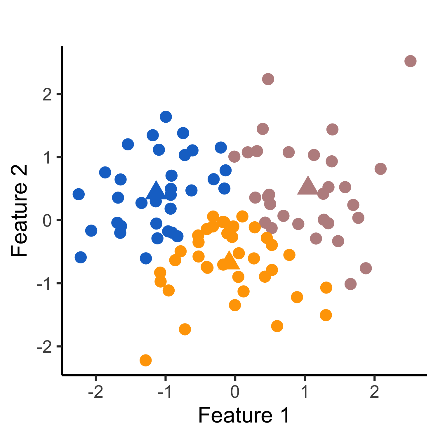
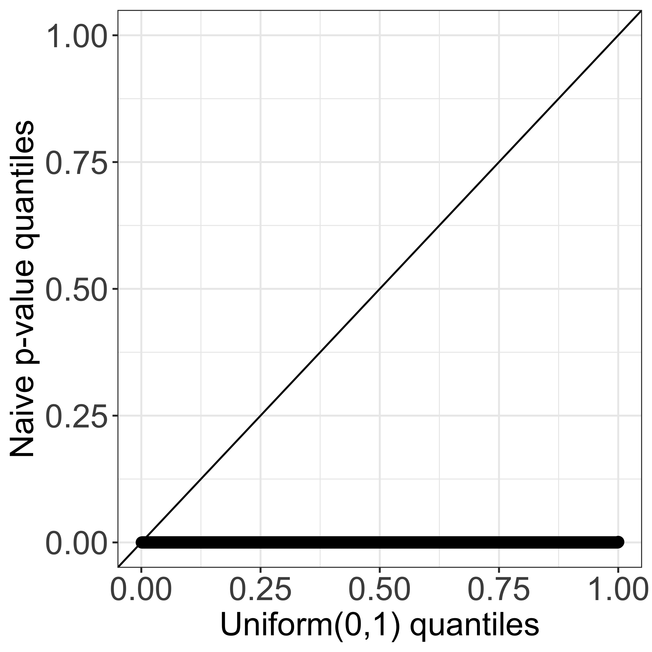
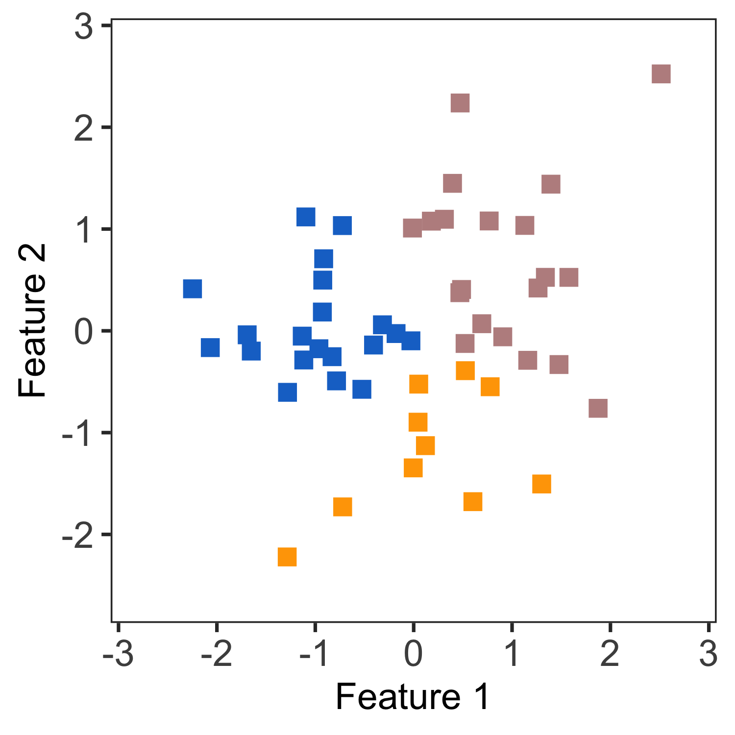
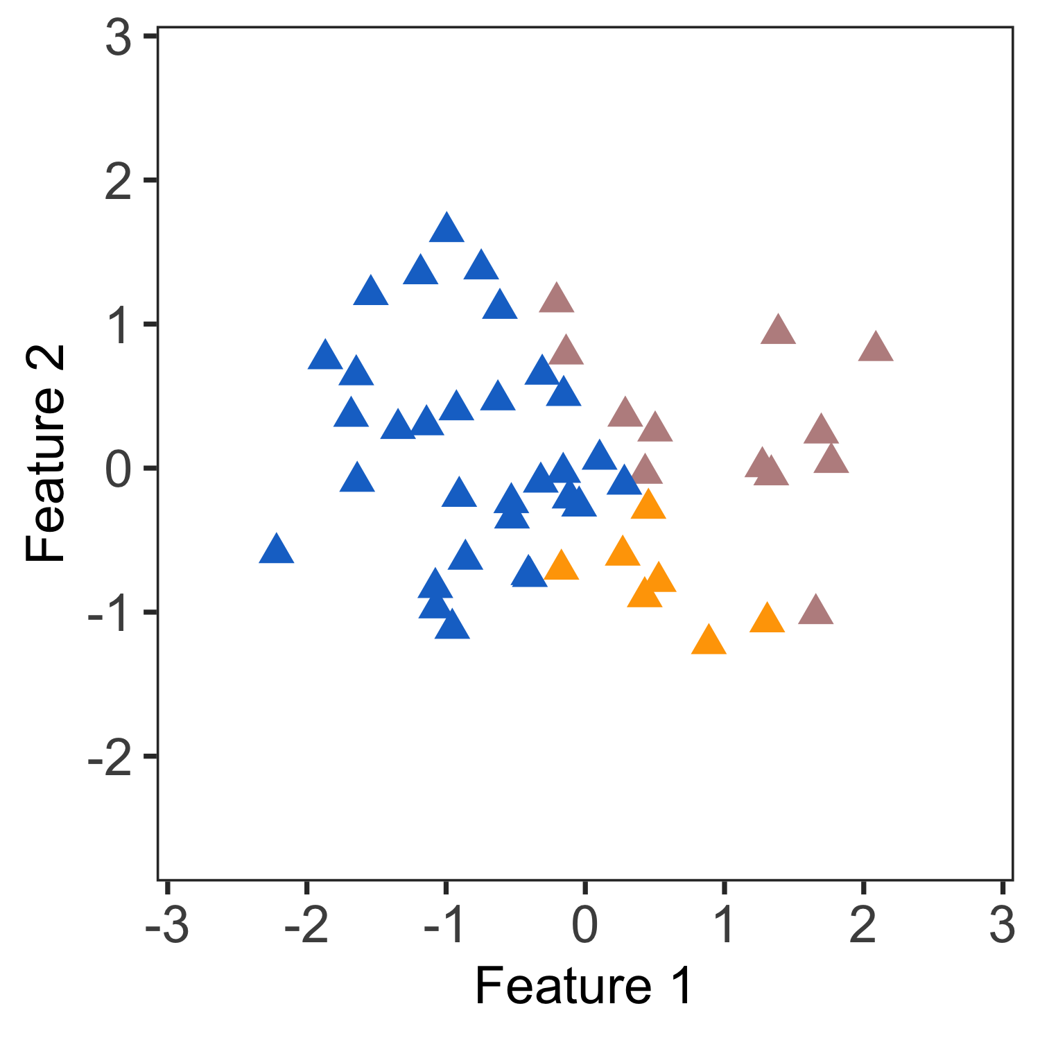
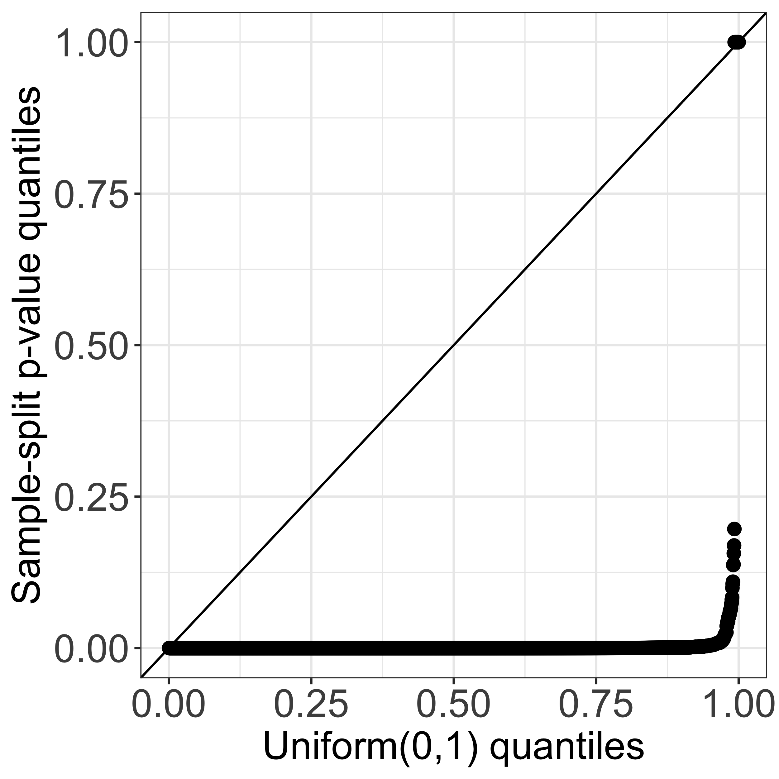
Notably, the problem of testing for a difference in means between two groups obtained via clustering cannot be easily overcome by sample splitting, as pointed out in Gao et al. (2020) and Zhang et al. (2019). To see why, we divide the observations into a training and a test set. We apply -means clustering on only the training set (left panel of Figure \arabicfigure), and then assign the test set observations to those clusters (to obtain the center panel of Figure \arabicfigure, we applied a 3-nearest neighbor classifier). Finally, we compute the naive -values (\arabicequation) only on the test set. Unfortunately, this approach does not work: while we clustered only the training data, we still used the test data to label the test observations, and consequently to construct the contrast vector in (\arabicequation). Therefore, the Wald test based on sample-splitting remains extremely anti-conservative, as shown in the right panel of Figure \arabicfigure, and does not lead to a valid test of in (\arabicequation).
In this paper, we develop a test of that controls the selective Type I error. That is, we wish to ensure that the probability of rejecting at level , given that holds and we decided to test it, is no greater than :
| (\arabicequation) |
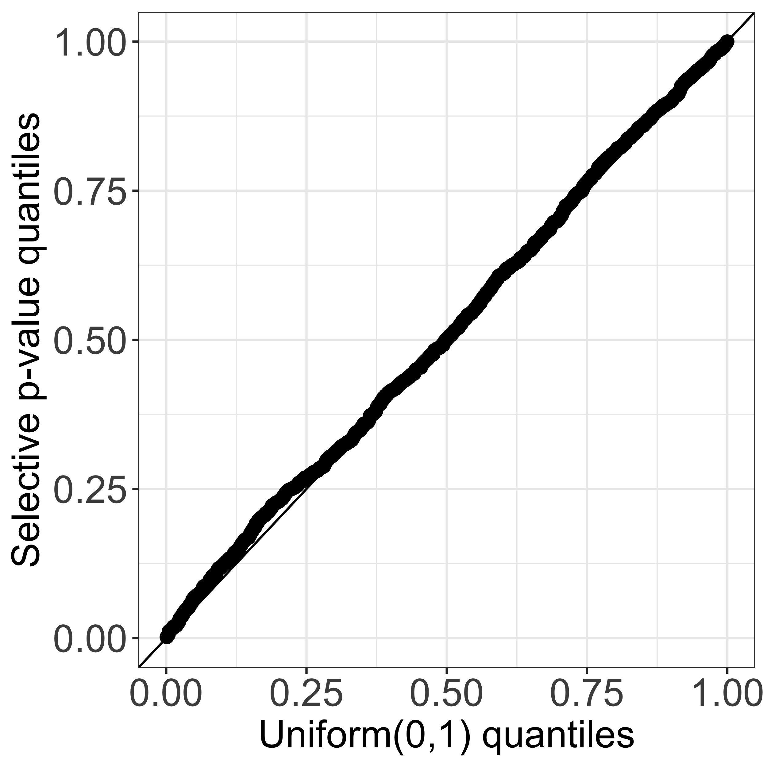
To develop the test, we leverage the selective inference framework, which has been applied extensively in high-dimensional linear modeling (Lee et al., 2016; Tibshirani et al., 2016; Fithian et al., 2014; Rügamer et al., 2022; Schultheiss et al., 2021; Taylor & Tibshirani, 2018; Charkhi & Claeskens, 2018; Yang et al., 2016; Loftus & Taylor, 2014), changepoint detection (Jewell et al., 2022; Hyun et al., 2021, 2018; Chen et al., 2021b; Le Duy & Takeuchi, 2021; Duy et al., 2020; Benjamini et al., 2019), and clustering (Zhang et al., 2019; Gao et al., 2020; Watanabe & Suzuki, 2021). The key insight behind selective inference is as follows: to obtain a valid test of , we need to condition on the aspect of the data that led us to test it. In our case, we chose to test the null hypothesis in (\arabicequation) because and were obtained via -means clustering. Therefore, we compute a -value conditional on the event that -means clustering yields and . This results in selective Type I error control (\arabicequation), as seen in the right panel of Figure \arabicfigure.
There is a rich literature on estimating and quantifying the uncertainty in the number of clusters (Li & Chen, 2010; Chen & Li, 2009; Chen et al., 2004; McLachlan et al., 2019; Dobriban, 2020), as well as assessing cluster stability and heterogeneity (Suzuki & Shimodaira, 2006; Kerr & Churchill, 2001; Kimes et al., 2017; Chung, 2020; Jin & Wang, 2016; Aw et al., 2021; Chung & Storey, 2015). Others have examined the asymptotic properties of clustering models from a Bayesian perspective (Guha et al., 2019; Nobile, 2004; Cai et al., 2020). In addition, -means clustering is a special case of the expectation-maximization algorithm, which allows us to tap into the active line of research on the statistical guarantees of the expectation-maximization algorithm (Zhang & Zhang, 2014; Wang et al., 2015; Cai et al., 2019; Yi & Caramanis, 2015; Balakrishnan et al., 2017). However, most prior work focused on scenarios where the number of clusters is correctly specified, and the estimated clusters memberships are close to the truth. By contrast, we are interested in a correctly-sized test for the null hypothesis (\arabicequation), even when do not correspond to true clusters. In addition, existing work often relies on asymptotic approximations and bootstrap resampling. Two recent exceptions include Zhang et al. (2019) and Gao et al. (2020), who took a selective inference approach and computed finite-sample -values for testing the difference in means between estimated clusters obtained via linear classification rules and hierarchical clustering, respectively. Our work is closest to Gao et al. (2020), and extends their framework to -means clustering. We provide an exact, finite-sample test of the difference in means between a pair of clusters estimated via -means clustering under model (\arabicequation), without the need for sample splitting.
Methods developed in this paper are implemented in the R package KmeansInference, available at https://github.com/yiqunchen/KmeansInference. Data and code for reproducing the results in this paper can be found at https://github.com/yiqunchen/KmeansInference-experiments.
Throughout this paper, we will use the following notational conventions. For a matrix , denotes the th row and denotes the th entry. For a vector , denotes its norm, and is the projection matrix onto the orthogonal complement of , i.e., , where is the -dimensional identity matrix. Moreover, if and otherwise, where is the -vector of zeros. We let and denote the inner product of two vectors and the indicator function, respectively.
\arabicsection Selective inference for k-means clustering
\arabicsection.\arabicsubsection A brief review of -means clustering
In this section, we review the -means clustering algorithm. Given samples and a positive integer , -means clustering partitions the samples into disjoint subsets by solving the following optimization problem:
| (\arabicequation) | ||||
It is not typically possible to solve for the global optimum in (LABEL:eq:k_means_objective) (Aloise et al., 2009). A number of algorithms are available to find a local optimum (Hartigan & Wong, 1979; Zha et al., 2002; Arthur & Vassilvitskii, 2007); one such approach is Lloyd’s algorithm (Lloyd, 1982), given in Algorithm 1. We first sample out of observations as initial centroids (step 1 in Algorithm 1). We then assign each observation to the closest centroid (step 2). Next, we iterate between re-computing the centroids and updating the cluster assignments (steps 3a. and 3b.) until the cluster assignments stop changing. The algorithm is guaranteed to converge to a local optimum (Hastie et al., 2001).
In what follows, we will sometimes use and rather than and to emphasize the dependence of the cluster labels and centroids on the data .
\arabicsection.\arabicsubsection A test of (\arabicequation) for clusters obtained via -means clustering
Here, we briefly review the proposal of Gao et al. (2020) for selective inference for hierarchical clustering, and outline a selective test for (\arabicequation) for -means clustering.
Gao et al. (2020) proposed a selective inference framework for testing hypotheses based on the output of a clustering algorithm. Let denote the clustering operator, i.e., a partition of the observations resulting from a clustering algorithm. Since in (\arabicequation) is chosen because , where are the two estimated clusters under consideration in (\arabicequation), Gao et al. (2020) proposed to reject if
| (\arabicequation) |
is small. In (\arabicequation), conditioning on eliminates the nuisance parameters and , where and (see, e.g., Section 3.1 of Fithian et al. (2014)). Gao et al. (2020) showed that the test that rejects when (\arabicequation) is below controls the selective Type I error at level , in the sense of (\arabicequation). Furthermore, under (\arabicequation), the conditional distribution of in (\arabicequation) is , truncated to a set. When the operator denotes hierarchical clustering, this set can be analytically characterized and efficiently computed, leading to an efficient algorithm for computing (\arabicequation).
We now extend these ideas to -means clustering (LABEL:eq:k_means_objective). Since the -means algorithm partitions all observations, it is natural to condition on the cluster assignments of all observations rather than just on . This leads to the -value
| (\arabicequation) |
where is the cluster assigned to the th observation at the final iteration of Algorithm 1. However, computing (\arabicequation) requires characterizing , which is not straightforward, and may necessitate enumerating over possibly an exponential number of intermediate cluster assignments for . Hence, we also condition on all of the intermediate clustering assignments in Algorithm 1:
| (\arabicequation) | |||
In (\arabicequation), is the cluster assigned to the th observation at the th iteration of Algorithm 1. Roughly speaking, this -value answers the question:
Assuming that there is no difference between the population means of and , what is the probability of observing such a large difference between their centroids, among all the realizations of that yield identical results in every iteration of the -means algorithm?
The -value in (\arabicequation) is the focus of this paper. We establish its key properties below.
Proposition \arabicsection.\arabictheorem.
Suppose that is a realization from (\arabicequation), and let . Then, under with defined in (\arabicequation),
| (\arabicequation) |
where is defined in (\arabicequation), and
| (\arabicequation) |
Moreover, the test that rejects when controls the selective Type I error at level , in the sense of (\arabicequation).
Proposition \arabicsection.\arabictheorem states that can be recast as the survival function of a scaled random variable, truncated to the set
| (\arabicequation) |
where is defined in (\arabicequation). Therefore, to compute , it suffices to characterize the set .
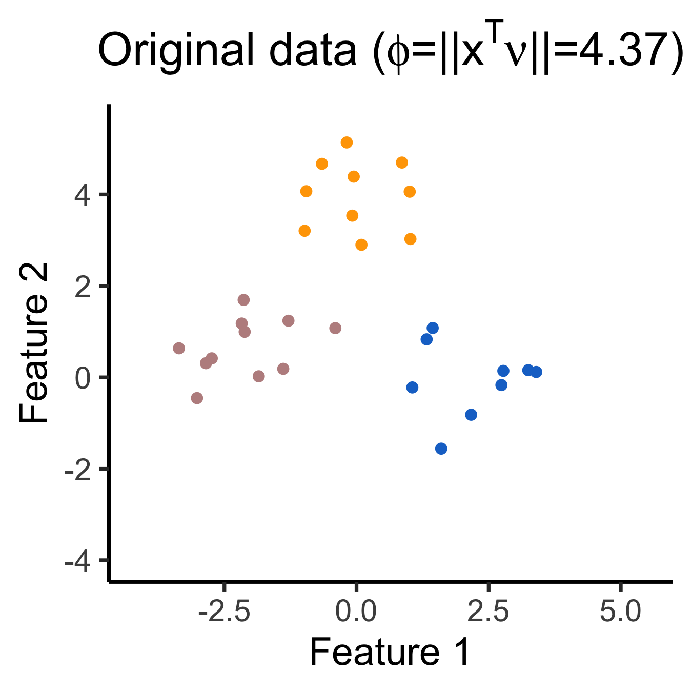

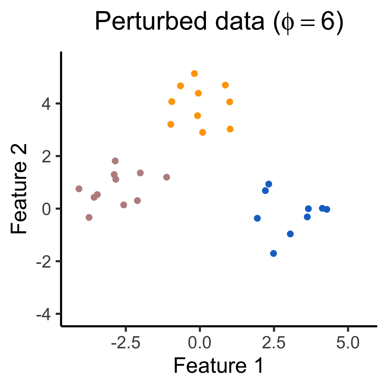
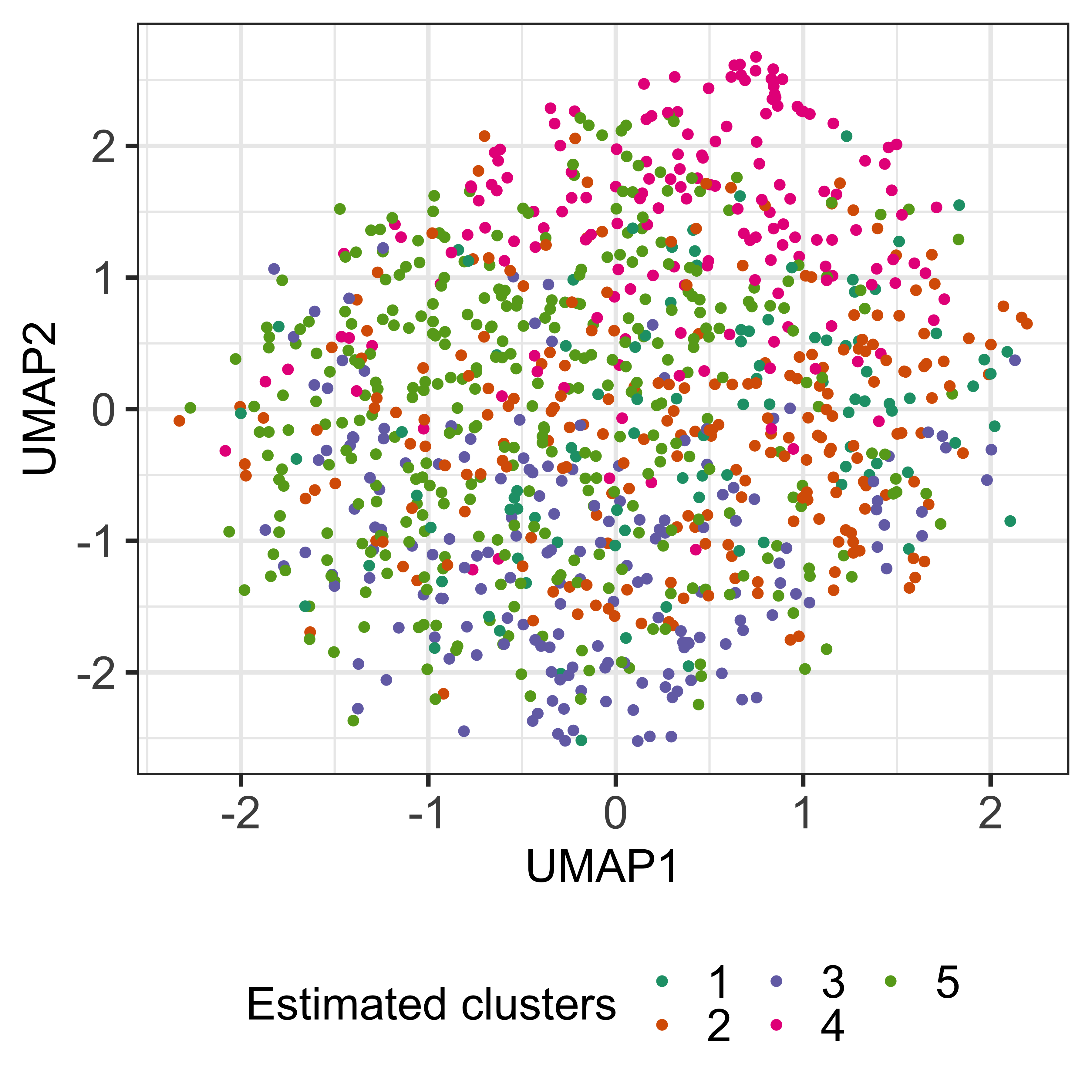
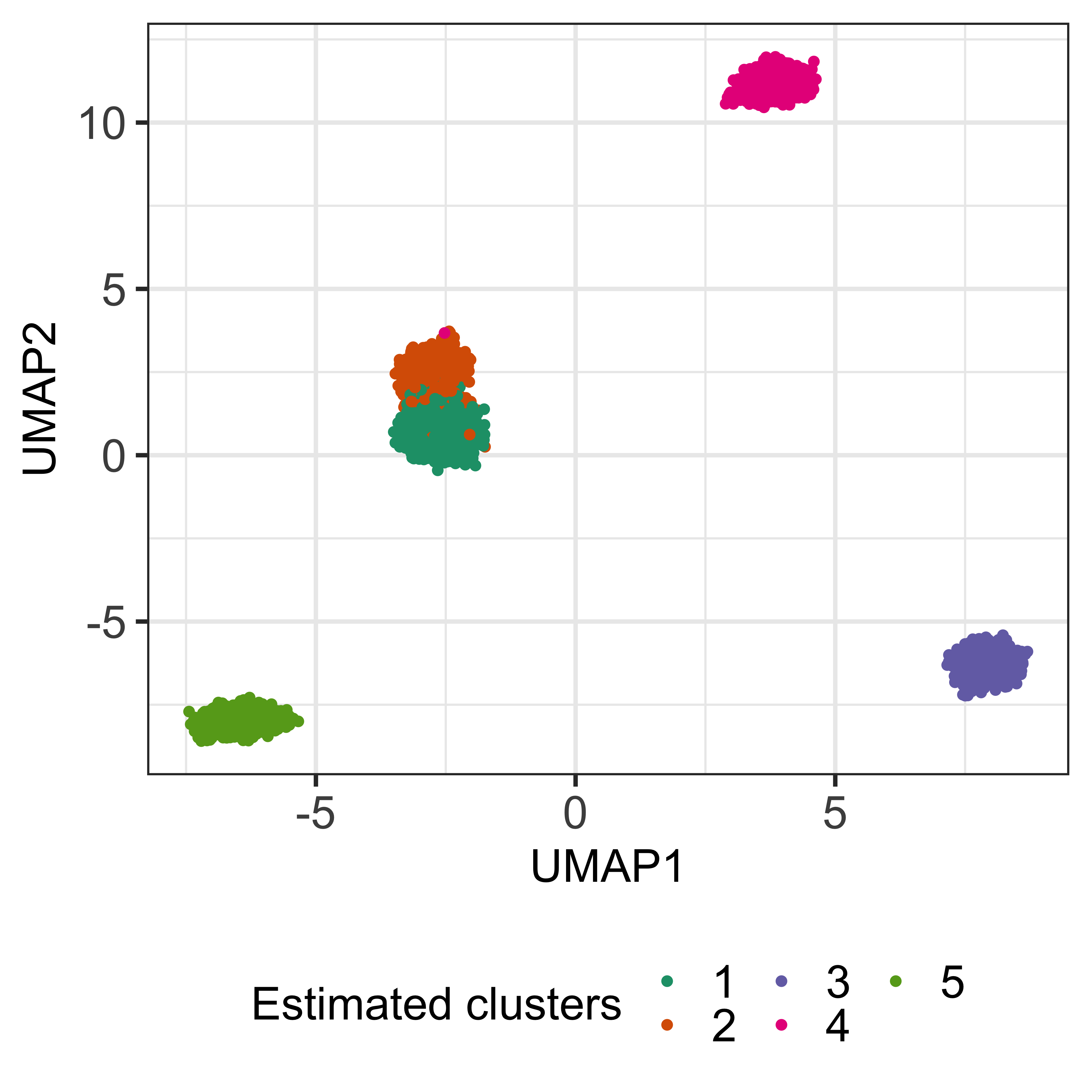
In (\arabicequation), results from applying a perturbation to the observed data , along the direction of , the difference between the two cluster centroids of interest. Figure \arabicfigure illustrates a realization of (\arabicequation) for -means clustering with . The left panel displays the observed data , which corresponds to with . Here, defined in (\arabicequation) was chosen to test the difference between (shown in pink) and (shown in blue). The center and right panels of Figure \arabicfigure display with and , respectively. In the center panel, with , the blue and pink clusters are “pushed together”, resulting in ; that is, there is no difference in empirical means between the two clusters under consideration. Applying -means clustering no longer results in these clusters. By contrast, in the right panel, with , the blue and pink clusters are “pulled apart” along the direction of , which results in an increased distance between the centroids of the blue and pink clusters, and -means clustering does yield the same clusters as on the original data. In this example, .
\arabicsection Computation of the selective p-value
In Section \arabicsection, we have shown that the -value (\arabicequation) involves the set in (\arabicequation). Here, we start with a high-level summary of our approach to characterizing in (\arabicequation). First, we rewrite as . Next, we consider the first term in the intersection: according to step 2. of Algorithm 1, for , if and only if for , the initial randomly-sampled centroid to which is closest coincides with the initial centroid to which is closest. This condition can be expressed using inequalities. Furthermore, the same intuition holds for the second term in the intersection, except that the centroids are a function of the cluster assignments in the previous iteration. We formalize this intuition in Proposition \arabicsection.\arabictheorem.
Proposition \arabicsection.\arabictheorem.
Suppose that we apply the -means clustering algorithm (Algorithm 1) to a matrix , to obtain clusters in at most steps. Define
| (\arabicequation) |
Then, for the set defined in (\arabicequation), we have that
| (\arabicequation) | |||
| (\arabicequation) |
Recall that denotes the cluster to which the th observation is assigned in step 3b. of Algorithm 1 during the th iteration, and that denotes the th centroid sampled from the data during step 1 of Algorithm 1. In words, Proposition \arabicsection.\arabictheorem says that can be expressed as the intersection of sets. Therefore, it suffices to characterize the sets in (\arabicequation) and (\arabicequation). We now present two lemmas.
Lemma \arabicsection.\arabictheorem (Lemma 2 in Gao et al. (2020)).
For in (\arabicequation) and in (\arabicequation), we have that , where , , and .
Lemma \arabicsection.\arabictheorem.
For in (\arabicequation), in (\arabicequation), and in (\arabicequation), we have that
, where
,
and .
It follows from Lemmas \arabicsection.\arabictheorem and \arabicsection.\arabictheorem that all of the inequalities in (\arabicequation) and (\arabicequation) are in fact quadratic in , with coefficients that can be analytically computed. Therefore, computing the set requires solving quadratic inequalities of .
Proposition \arabicsection.\arabictheorem.
Suppose that we apply the -means clustering algorithm (Algorithm 1) to a matrix , to obtain clusters in at most steps. Then, the set defined in (\arabicequation) can be computed in operations.
\arabicsection Extensions
\arabicsection.\arabicsubsection Non-spherical covariance matrix
Thus far, we have assumed that the observed data is a realization of (\arabicequation), which implies that . However, this assumption is often violated in practice. For example, expression levels of genes are highly correlated, and neighbouring pixels in an image tend to be more similar. For a known positive definite matrix , we now let
| (\arabicequation) |
Under (\arabicequation), we can whiten the data by applying the transformation (Bell & Sejnowski, 1997), where is the unique symmetric positive definite square root of (Horn & Johnson, 2012). Note that . Moreover, as , testing the null hypothesis in (\arabicequation) is equivalent to testing
| (\arabicequation) |
Therefore, to get a correctly-sized test under model (\arabicequation), we can simply carry out our proposal in Section \arabicsection on the transformed data instead of the original data .
Instead of applying the whitening transformation, we can directly accommodate a known covariance matrix by considering the following extension of in (\arabicequation):
| (\arabicequation) | ||||
Proposition \arabicsection.\arabictheorem.
Suppose that is a realization from (\arabicequation), and let . Then, under with defined in (\arabicequation),
| (\arabicequation) |
where is defined in (\arabicequation). Furthermore, the test that rejects when controls the selective Type I error at level .
In addition, we can adapt the results in Section \arabicsection to compute the set by modifying the results in Lemmas \arabicsection.\arabictheorem and \arabicsection.\arabictheorem. Details are in Section A.\arabicsubsection of the Appendix.
\arabicsection.\arabicsubsection Unknown variance
When is unknown, we can plug in an estimate in (\arabicequation):
| (\arabicequation) |
where . If we use a consistent estimator of , then a test based on the -value in (\arabicequation) provides selective Type I error control (\arabicequation) asymptotically.
Proposition \arabicsection.\arabictheorem.
For suppose that . Let be a realization from and let be the cluster to which the th observation is assigned during the th iteration of step 3b. in Algorithm 1. Consider the sequence of null hypotheses , where defined in (\arabicequation) is the contrast vector resulting from applying -means clustering on . Suppose that (i) is a consistent estimator of , i.e., for all ; and (ii) there exists such that . Then, for all , we have that .
In practice, we propose to use the following estimator of (Huber, 1981):
| (\arabicequation) |
where is obtained from subtracting the median of each column in , and is the median of the distribution. If is sparse, i.e., is small, then (\arabicequation) is consistent with appropriate assumptions; see Appendix A.\arabicsubsection.
\arabicsection Simulation study
\arabicsection.\arabicsubsection Overview
Throughout this section, we consider testing the null hypothesis , where, unless otherwise stated, defined in is based on a randomly-chosen pair of clusters and from -means clustering. We consider four -values: in (\arabicequation), in (\arabicequation), in (\arabicequation) with defined in (\arabicequation), and in (\arabicequation) with , where . In the simulations that follow, we compare the selective Type I error (\arabicequation) and power of the tests that reject when these -values are less than .
\arabicsection.\arabicsubsection Selective Type I error under the global null
We generate data from (\arabicequation) with ; therefore, in (\arabicequation) holds for any pair of estimated clusters. We simulate 3,000 datasets with , , and .
For each simulated dataset, we apply -means clustering with , and then compute , , , and for a randomly-chosen pair of clusters. Figure \arabicfigure displays the observed -value quantiles versus the Uniform(0,1) quantiles. We see that for all values of , (i) the naive -values in (\arabicequation) are stochastically smaller than a Uniform(0,1) random variable, and the test based on leads to an inflated Type I error rate; (ii) tests based , , and control the selective Type I error rate in the sense of (\arabicequation).

\arabicsection.\arabicsubsection Conditional power and detection probability
In this section, we show that the tests based on our proposal (, , and ) have substantial power to reject when it is not true. We generate data from (\arabicequation) with and
| (\arabicequation) |
Here, we can think of as the “true clusters”. Moreover, these clusters are equidistant in the sense that the pairwise distance between each pair of population means is . Recall that we test in (\arabicequation) for a pair of estimated clusters and , which may not be true clusters. Hence, we will separately consider the conditional power and detection probability of our proposed tests (Gao et al., 2020; Jewell et al., 2022; Hyun et al., 2021). The conditional power is the probability of rejecting in (\arabicequation), given that and are true clusters. Given simulated datasets, we estimate it as
| (\arabicequation) |
where are true clusters, and and correspond to the -value and clusters under consideration for the th simulated dataset. Because the quantity in (\arabicequation) conditions on the event that and are true clusters, we also estimate how often that event occurs:
| (\arabicequation) |

We generate datasets from (\arabicequation) with and . For each simulated dataset, we apply -means clustering with and reject if , , or is less than . In Figure \arabicfigure, the left panel displays the detection probability (\arabicequation) of -means clustering as a function of in (\arabicequation), and the right panel displays the conditional power (\arabicequation) for the tests based on , , and . Under model (\arabicequation), the detection probability and conditional power increase as a function of in (\arabicequation) for all values of . For a given value of , a larger value of leads to lower detection probability and conditional power. The conditional power is not displayed for because the true clusters were never recovered in simulation. Moreover, for a given value of and , the test based on has the highest conditional power, followed closely by the test based on . Using in leads to a less powerful test, especially for large values of . This is because is a conservative estimator of in (\arabicequation), and its bias is an increasing function of , the distance between true clusters. By contrast, is a consistent estimator under model (\arabicequation) (see Appendix A.\arabicsubsection).
As an alternative to the conditional power in (\arabicequation), in Appendix A.\arabicsubsection, we consider a notion of power that does not condition on having correctly estimated the true clusters.
\arabicsection Real data applications
\arabicsection.\arabicsubsection Palmer Penguins (Horst et al., 2020)
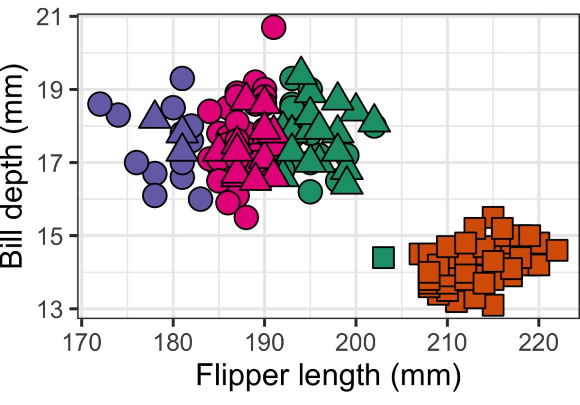
Here we analyze the Palmer penguins dataset from the palmerpenguins package in R (Horst et al., 2020). We consider the 165 female penguins with complete observations, and apply -means clustering with to two of the collected features: bill depth and flipper length. Figure \arabicfigure displays the estimated clusters.
| 0.24 | ||
| 0.10 |
We assess the equality of the means of each pair of estimated clusters using in (\arabicequation) and in (\arabicequation) with defined in (\arabicequation). The results are in Figure \arabicfigure. The naive p-values are small for all pairs of estimated clusters, even when the underlying species distributions are nearly identical (e.g., both clusters 1 and 4 are a mix of Chinstrap and Adelie penguins). By contrast, our proposal results in large -values when testing for a difference in means between clusters composed of the same species (clusters 1 and 4, clusters 3 and 4), and small -values when the clusters correspond to different species (e.g., clusters 1 and 2, clusters 2 and 3).
\arabicsection.\arabicsubsection MNIST Dataset (Lecun et al., 1998)
In this section, we apply our method to the MNIST dataset (Lecun et al., 1998), which consists of 60,000 gray-scale images of handwritten digits. Each image has an accompanying label in , and is stored as a matrix that takes on values in . We first divide the entries of all the images by 255. Next, since there is no variation in the peripheral pixels of the images (Gallaugher & McNicholas, 2018), which violates model (\arabicequation), we add an independent perturbation to each element of the image. Finally, we vectorize each image to obtain a vector .
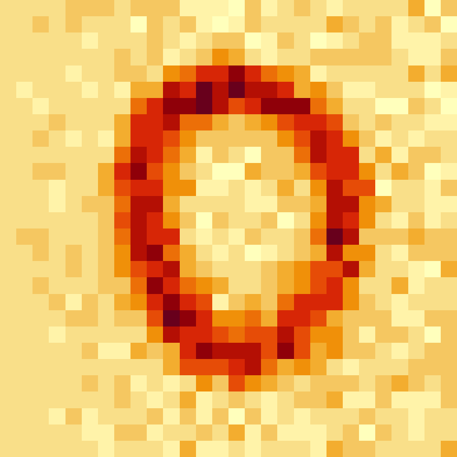
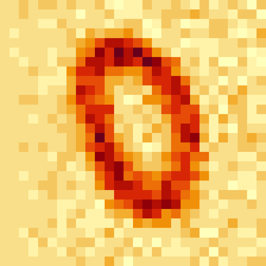
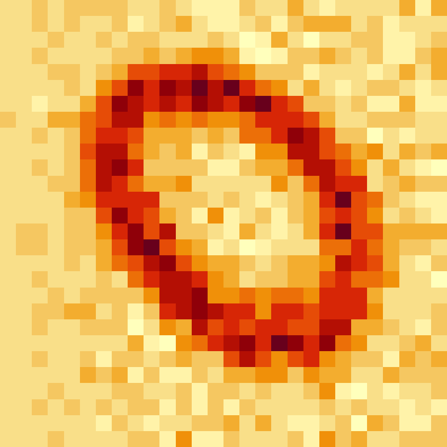
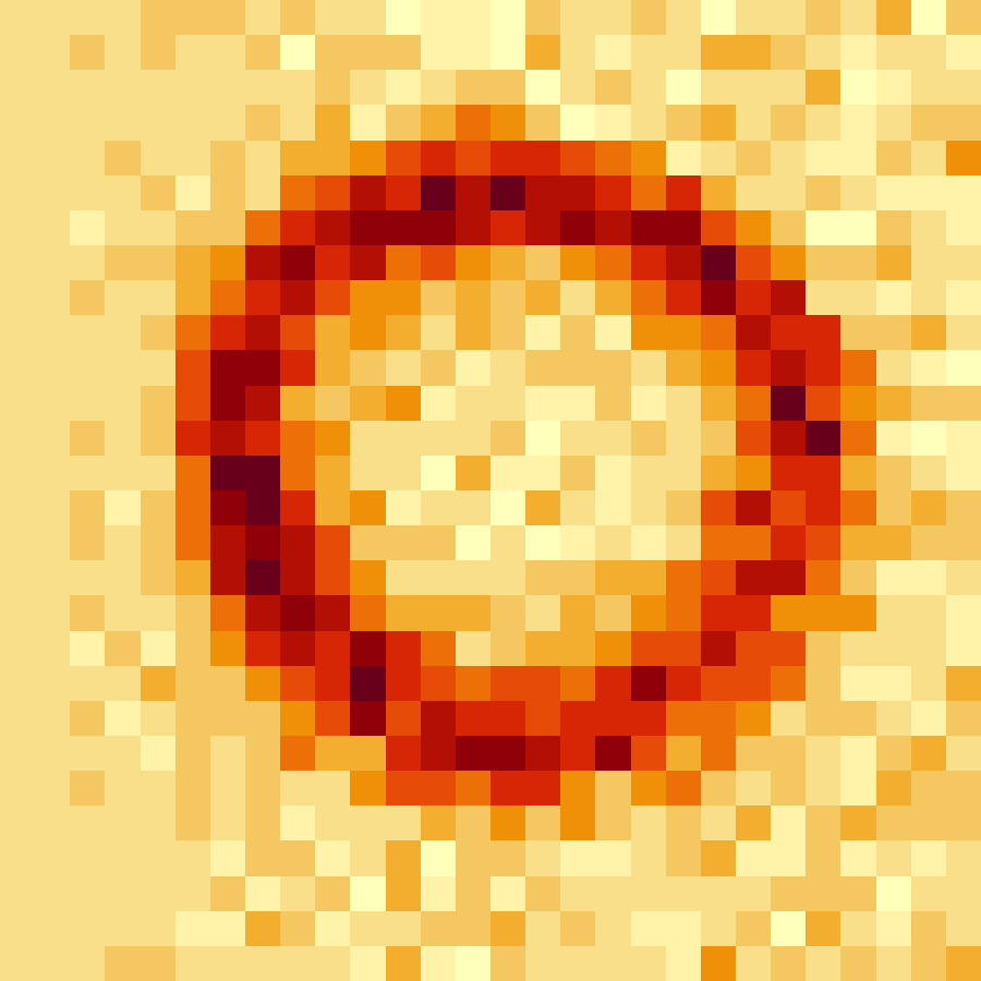
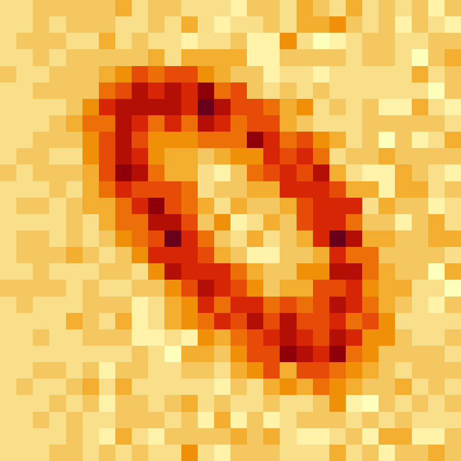
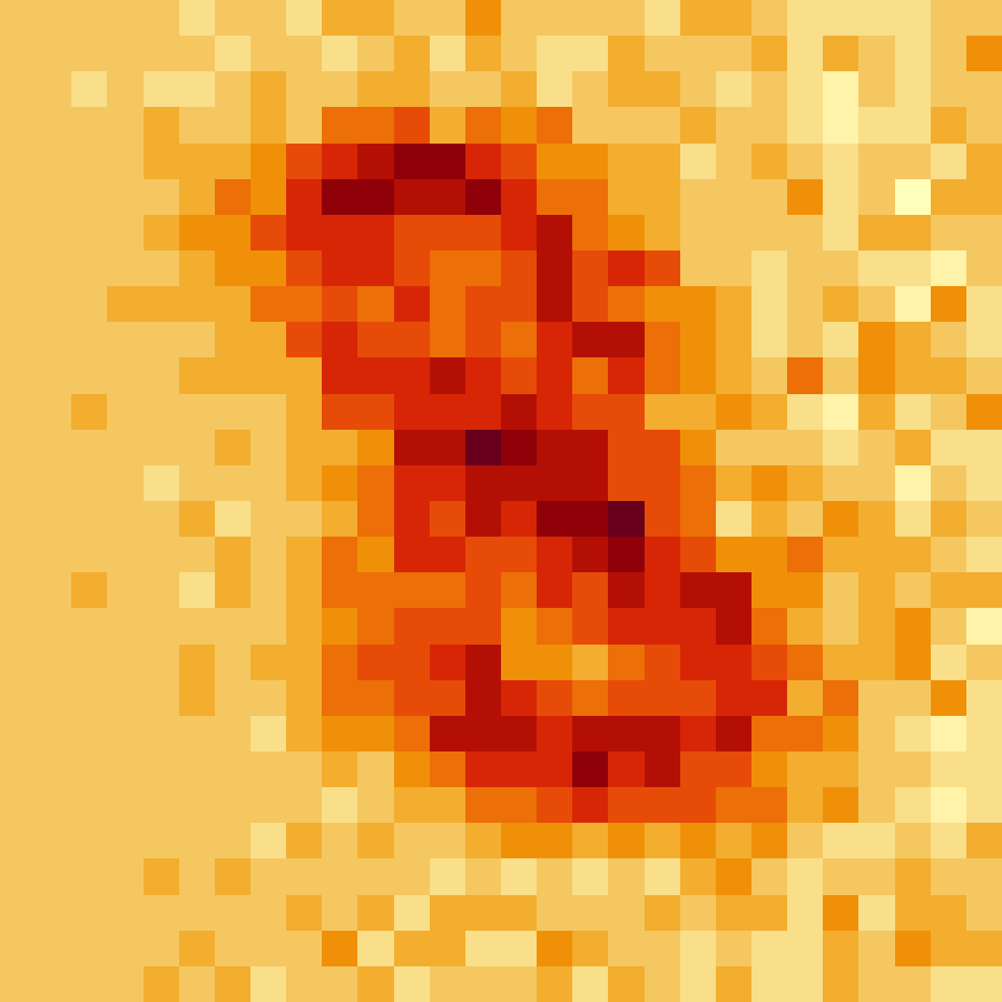
| “No cluster” | ||||
| “Cluster” | ||||
We first construct a “no cluster” dataset by randomly sampling 1,500 images of the 0s; thus, and . To de-correlate the pixels in each image, we whitened the data (see Section \arabicsection.\arabicsubsection) using as in prior work (Coates & Ng, 2012), where is the eigenvalue decomposition of the sample covariance matrix.
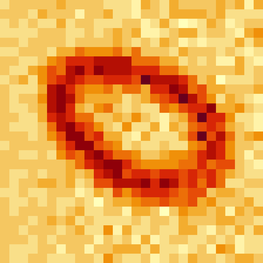
We apply -means clustering with . The centroids are displayed in the top left panel of Figure \arabicfigure. For each pair of estimated clusters, we compute the -values and (see Figure \arabicfigure). The naive -values are extremely small for all pairs of clusters under consideration, despite the resemblance of the centroids. By contrast, our approach yields modest -values, congruent with the visual resemblance of the centroids. In addition, for the most part, the pairs for which is small are visually quite different (e.g., clusters 1 and 2, clusters 1 and 5, and clusters 4 and 5).
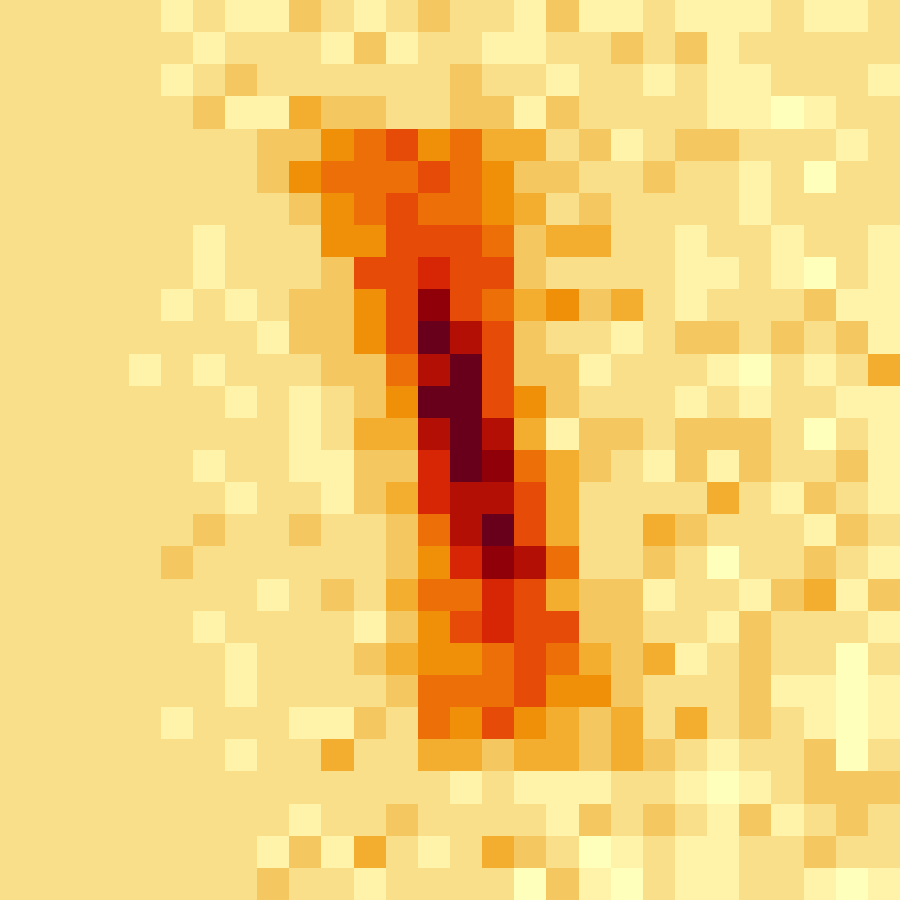
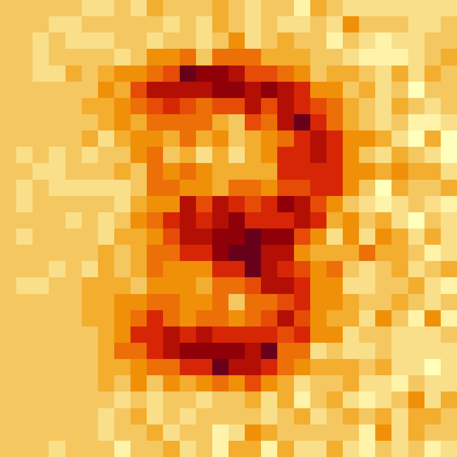
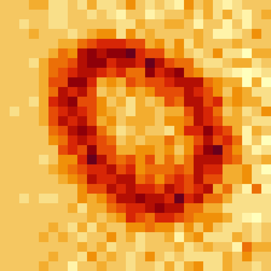
To demonstrate the power of the test based on , we also generated a “cluster” dataset by sampling 500 images each from digits and 8; thus, and . We again whitened the data to obtain uncorrelated features. After applying -means clustering with , we obtain four clusters that roughly correspond to four digits: cluster 1, 94.0% digit 1; cluster 2, 72.4% digit 3; cluster 3, 83.6% digit 0; cluster 4, 62.4% digit 8 (see the bottom left panel of Figure \arabicfigure). Results from testing for a difference in means for each pair of clusters using and are in Figure \arabicfigure. Both sets of -values are small on this “cluster” dataset.
\arabicsection.\arabicsubsection Single-cell RNA-sequencing data (Zheng et al., 2017)
In this section, we apply our proposal to single-cell RNA-sequencing data collected by Zheng et al. (2017). Single-cell RNA-sequencing quantifies gene expression abundance at the resolution of single cells, thereby revealing cell-to-cell heterogeneity in transcription and allowing for the identification of cell types and marker genes. In practice, biologists often cluster the cells to identify putative cell types, and then perform a differential expression analysis, i.e., they test for a difference in gene expression between two clusters (Stuart et al., 2019; Lähnemann et al., 2020; Grün et al., 2015). Because this approach ignores the fact that the clusters were estimated from the same data used for testing, it does not control the selective Type I error.
Zheng et al. (2017) profiled 68,000 peripheral blood mononuclear cells, and classified them based on their match to the expression profiles of 11 reference transcriptomes from known cell types. We consider the classified cell types to be the “ground truth”, and use this information to demonstrate that our proposal in Section \arabicsection yields reasonable results.
As in prior work (Gao et al., 2020; Duò et al., 2018), we first excluded cells with low numbers of expressed genes or total counts, as well as cells in which a large percentage of the expressed genes are mitochondrial. We then divided the counts for each cell by the total sum of counts in that cell. Finally, we applied a transformation with a pseudo-count of 1 to the expression data, and considered only the subset of 500 genes with the largest average expression levels pre-normalization.
We applied the aforementioned pre-processing pipeline separately to memory T cells () and a mixture of five types of cells (memory T cells, B cells, naive T cells, natural killer cells, and monocytes; ).
To investigate the selective Type I error in the absence of true clusters, we first constructed a “no cluster” dataset by randomly sampling 1,000 out of 10,224 memory T cells after pre-processing (thus, and ). Since the gene expression levels are highly correlated, we first whitened the data as described in Section \arabicsection.\arabicsubsection by plugging in (Coates & Ng, 2012), where is the eigenvalue decomposition of the sample covariance matrix.
We applied -means clustering to the transformed data with , and obtained five clusters consisting of 97, 223, 172, 165, and 343 cells, respectively (see Figure \arabicfigure left panel in Appendix A.\arabicsubsection). For each pair of estimated clusters, we computed the -values and . The results are displayed in the top panel of Table \arabicsection.\arabicsubsection. On this dataset, the naive p-values are extremely small for all pairs of estimated clusters, while our proposed -values are quite large. In particular, at , the test based on concludes that all five estimated clusters correspond to distinct cell types (even after multiplicity correction), whereas our approach does not reject the null hypothesis that the expression levels (and thus cell types) are, in fact, the same between estimated clusters. Because this “no cluster” dataset consists only of memory T cells, we believe that conclusion based on aligns better with the underlying biology.
P-values in (\arabicequation) and in (\arabicequation) with defined in (\arabicequation) corresponding to the null hypothesis that the means of two estimated clusters are equal, for each pair of estimated clusters in the “no cluster” (top) and the “cluster” datasets (bottom) 0.30 0.43 0.12 0.12 0.005 0.04 0.05
Next, we construct a “cluster” dataset by randomly sampling 400 each of memory T cells, B cells, naive T cells, natural killer cells, and monocytes from the cells; thus, and . After whitening the data, we applied -means clustering to obtain five clusters. We see that these clusters approximately correspond to the five different cell types (cluster 1: 82.5% naive T cells; cluster 2: 95.3% memory T cells; cluster 3: 99.2% B cells; cluster 4: 91.5% nature killer cells; cluster 5: 83.3% monocytes); estimated clusters are visualized in the right panel of Figure \arabicfigure in Appendix A.\arabicsubsection. We evaluate the -values and for all pairs of estimated clusters, and display results in the bottom panel of Table \arabicsection.\arabicsubsection. Both sets of -values are extremely small on this dataset, which suggests that the test based on our -value has substantial power to reject the null hypothesis when it does not hold.
\arabicsection Discussion
We have proposed a test for a difference in means between two clusters estimated from -means clustering, under (\arabicequation). Here, we outline several future research directions.
While the -value in (\arabicequation) leads to selective Type I error control, it conditions on more information than is used to construct the hypothesis in (\arabicequation). In practice, data analysts likely only make use of the final cluster assignments (leading to the -value in (\arabicequation)), as opposed to all the intermediate assignments (leading to the -value in (\arabicequation)). Empirically, conditioning on too much information results in a loss of power (Fithian et al., 2014; Jewell et al., 2022; Liu et al., 2018). In future work, we will investigate the possibility of leveraging recent developments in selective inference (Chen et al., 2021a; Le Duy & Takeuchi, 2021; Jewell et al., 2022) to compute the “ideal” -value (\arabicequation).
We could also consider extending our proposal to other data generating models. The normality assumption in (\arabicequation) is critical to the proof of Proposition \arabicsection.\arabictheorem, because it guarantees that under in (\arabicequation), , , and are pairwise independent. However, this normality assumption is often violated in practice; for instance, in single-cell genomics, the data are count-valued and the variance of gene expression levels varies drastically with the mean expression levels of that gene (Stuart et al., 2019; Eling et al., 2018). This has motivated some authors to work with alternative models for gene expression including Poisson (Witten, 2011), negative binomial (Risso et al., 2018), and curved normal (Lin et al., 2021). To extend our framework to other exponential family distributions, we may be able to leverage recent proposals to decompose into and such that both and have a known, computationally-tractable distribution (Rasines & Alastair Young, 2021; Leiner et al., 2021).
\arabicsection Acknowledgments
This work was partially supported by National Institutes of Health grants and a Simons Investigator Award to Daniela Witten.
References
- Aizarani et al. (2019) Aizarani, N., Saviano, A., Sagar, Mailly, L., Durand, S., Herman, J. S., Pessaux, P., Baumert, T. F. & Grün, D. (2019). A human liver cell atlas reveals heterogeneity and epithelial progenitors. Nature 572, 199–204.
- Aloise et al. (2009) Aloise, D., Deshpande, A., Hansen, P. & Popat, P. (2009). NP-hardness of Euclidean sum-of-squares clustering. Machine Learning 75, 245–248.
- Arthur & Vassilvitskii (2007) Arthur, D. & Vassilvitskii, S. (2007). k-means++: the advantages of careful seeding. In Proceedings of the Eighteenth Annual ACM-SIAM Symposium On Discrete Algorithms, SODA ’07. USA: Society for Industrial and Applied Mathematics.
- Avella-Medina et al. (2018) Avella-Medina, M., Battey, H. S., Fan, J. & Li, Q. (2018). Robust estimation of high-dimensional covariance and precision matrices. Biometrika 105, 271–284.
- Aw et al. (2021) Aw, A. J., Spence, J. P. & Song, Y. S. (2021). A flexible and robust non-parametric test of exchangeability. arXiv , 2109.15261.
- Balakrishnan et al. (2017) Balakrishnan, S., Wainwright, M. J. & Yu, B. (2017). Statistical guarantees for the EM algorithm: From population to sample-based analysis. The Annals of Statistics 45, 77–120.
- Bell & Sejnowski (1997) Bell, A. J. & Sejnowski, T. J. (1997). The “independent components” of natural scenes are edge filters. Vision Research 37, 3327–3338.
- Belomestny et al. (2019) Belomestny, D., Trabs, M. & Tsybakov, A. B. (2019). Sparse covariance matrix estimation in high-dimensional deconvolution. Bernoulli 25, 1901 – 1938.
- Benjamini et al. (2019) Benjamini, Y., Taylor, J. & Irizarry, R. A. (2019). Selection-corrected statistical inference for region detection with high-throughput assays. Journal of the American Statistical Association 114, 1351–1365.
- Bickel & Levina (2008) Bickel, P. J. & Levina, E. (2008). Covariance regularization by thresholding. The Annals of Statistics 36, 2577–2604.
- Bilodeau & Brenner (1999) Bilodeau, M. & Brenner, D. (1999). Theory of Multivariate Statistics. Springer, New York, NY.
- Bourgon (2020) Bourgon, R. (2020). intervals: Tools for working with points and intervals. https://cran.rstudio.com/web/packages/intervals/index.html. Accessed: 2022-2-11.
- Button (2019) Button, K. S. (2019). Double-dipping revisited. Nature Neuroscience 22, 688–690.
- Cai et al. (2020) Cai, D., Campbell, T. & Broderick, T. (2020). Finite mixture models do not reliably learn the number of components. arXiv , 2007.04470.
- Cai et al. (2019) Cai, T. T., Ma, J. & Zhang, L. (2019). CHIME: Clustering of high-dimensional gaussian mixtures with EM algorithm and its optimality. The Annals of Statistics 47, 1234–1267.
- Charkhi & Claeskens (2018) Charkhi, A. & Claeskens, G. (2018). Asymptotic post-selection inference for the Akaike information criterion. Biometrika 105, 645–664.
- Chen et al. (2004) Chen, H., Chen, J. & Kalbfleisch, J. D. (2004). Testing for a finite mixture model with two components. J. R. Stat. Soc. Series B Stat. Methodol. 66, 95–115.
- Chen & Li (2009) Chen, J. & Li, P. (2009). Hypothesis test for normal mixture models: The EM approach. The Annals of Statistics 37, 2523–2542.
- Chen et al. (2018) Chen, M., Gao, C. & Ren, Z. (2018). Robust covariance and scatter matrix estimation under Huber’s contamination model. Annals of Statistics 46.
- Chen & Bien (2020) Chen, S. & Bien, J. (2020). Valid inference corrected for outlier removal. J. Comput. Graph. Stat. 29, 323–334.
- Chen et al. (2021a) Chen, Y., Jewell, S. & Witten, D. (2021a). More powerful selective inference for the graph fused lasso. arXiv , 2109.10451.
- Chen et al. (2021b) Chen, Y. T., Jewell, S. W. & Witten, D. M. (2021b). Quantifying uncertainty in spikes estimated from calcium imaging data. To appear in Biostatistics .
- Chung (2020) Chung, N. C. (2020). Statistical significance of cluster membership for unsupervised evaluation of cell identities. Bioinformatics 36, 3107–3114.
- Chung & Storey (2015) Chung, N. C. & Storey, J. D. (2015). Statistical significance of variables driving systematic variation in high-dimensional data. Bioinformatics 31, 545–554.
- Coates & Ng (2012) Coates, A. & Ng, A. Y. (2012). Learning feature representations with K-Means. In Neural Networks: Tricks of the Trade: Second Edition, G. Montavon, G. B. Orr & K.-R. Müller, eds. Berlin, Heidelberg: Springer Berlin Heidelberg, pp. 561–580.
- Comminges et al. (2021) Comminges, L., Collier, O., Ndaoud, M. & Tsybakov, A. B. (2021). Adaptive robust estimation in sparse vector model. Annals of Statistics 49.
- Dobriban (2020) Dobriban, E. (2020). Permutation methods for factor analysis and PCA. Annals of Statistics 48.
- Doughty & Kerkhoven (2020) Doughty, T. & Kerkhoven, E. (2020). Extracting novel hypotheses and findings from RNA-seq data. FEMS Yeast Res. 20.
- Duò et al. (2018) Duò, A., Robinson, M. D. & Soneson, C. (2018). A systematic performance evaluation of clustering methods for single-cell RNA-seq data. F1000Research 7, 1141.
- Duy et al. (2020) Duy, V. N. L., Toda, H., Sugiyama, R. & Takeuchi, I. (2020). Computing valid p-value for optimal changepoint by selective inference using dynamic programming. arXiv , 2002.09132.
- Eling et al. (2018) Eling, N., Richard, A. C., Richardson, S., Marioni, J. C. & Vallejos, C. A. (2018). Correcting the mean-variance dependency for differential variability testing using single-cell RNA sequencing data. Cell Systems 7, 284–294.e12.
- Fithian et al. (2014) Fithian, W., Sun, D. & Taylor, J. (2014). Optimal inference after model selection. arXiv , 1410.2597.
- Friederich et al. (2020) Friederich, P., Krenn, M., Tamblyn, I. & Aspuru-Guzik, A. (2020). Scientific intuition inspired by machine learning generated hypotheses. arXiv , 2010.14236.
- Gallaugher & McNicholas (2018) Gallaugher, M. P. B. & McNicholas, P. D. (2018). Finite mixtures of skewed matrix variate distributions. Pattern Recognition 80, 83–93.
- Gao et al. (2020) Gao, L. L., Bien, J. & Witten, D. (2020). Selective inference for hierarchical clustering. arXiv , 2012.02936.
- Grün et al. (2015) Grün, D., Lyubimova, A., Kester, L., Wiebrands, K., Basak, O., Sasaki, N., Clevers, H. & van Oudenaarden, A. (2015). Single-cell messenger RNA sequencing reveals rare intestinal cell types. Nature 525, 251–255.
- Guha et al. (2019) Guha, A., Ho, N. & Nguyen, X. (2019). On posterior contraction of parameters and interpretability in bayesian mixture modeling. arXiv , 1901.05078.
- Han & Liu (2014) Han, F. & Liu, H. (2014). Scale-invariant sparse PCA on high dimensional meta-elliptical data. Journal of the American Statistical Association 109, 275–287.
- Hand & Adams (2015) Hand, D. J. & Adams, N. M. (2015). Data Mining. Chichester, UK: John Wiley & Sons, Ltd, pp. 1–7.
- Hartigan & Wong (1979) Hartigan, J. A. & Wong, M. A. (1979). Algorithm AS 136: A k-means clustering algorithm. Journal of the Royal Statistical Society. Series C, Applied statistics 28, 100–108.
- Hastie et al. (2001) Hastie, Trevor., Hastie, Trevor., Tibshirani, Robert., Friedman & H., J. (2001). The Elements of Statistical Learning : data mining, inference, and prediction. New York: Springer.
- Horn & Johnson (2012) Horn, R. A. & Johnson, C. R. (2012). Matrix Analysis. Cambridge University Press, 2nd ed.
- Horst et al. (2020) Horst, A. M., Hill, A. P. & Gorman, K. B. (2020). palmerpenguins: Palmer Archipelago (Antarctica) penguin data. R package version 0.1.0.
- Huber (1981) Huber, P. J. (1981). Robust Statistics. John Wiley & Sons.
- Hung & Fithian (2020) Hung, K. & Fithian, W. (2020). Statistical methods for replicability assessment. The Annals of Applied Statistics 14, 1063–1087.
- Hyun et al. (2018) Hyun, S., G’Sell, M. & Tibshirani, R. J. (2018). Exact post-selection inference for the generalized lasso path. Electron. J. Stat. 12, 1053–1097.
- Hyun et al. (2021) Hyun, S., Lin, K. Z., G’Sell, M. & Tibshirani, R. J. (2021). Post-selection inference for changepoint detection algorithms with application to copy number variation data. Biometrics .
- Jewell et al. (2022) Jewell, S., Fearnhead, P. & Witten, D. (2022). Testing for a change in mean after changepoint detection. To appear in J. R. Stat. Soc. Series B Stat. Methodol. .
- Jin & Wang (2016) Jin, J. & Wang, W. (2016). Influential features PCA for high dimensional clustering. The Annals of Statistics 44, 2323–2359.
- Kerr & Churchill (2001) Kerr, M. K. & Churchill, G. A. (2001). Bootstrapping cluster analysis: assessing the reliability of conclusions from microarray experiments. Proceedings of the National Academy of Sciences of the United States of America 98, 8961–8965.
- Kimes et al. (2017) Kimes, P. K., Liu, Y., Neil Hayes, D. & Marron, J. S. (2017). Statistical significance for hierarchical clustering. Biometrics 73, 811–821.
- Kriegeskorte et al. (2009) Kriegeskorte, N., Simmons, W. K., Bellgowan, P. S. F. & Baker, C. I. (2009). Circular analysis in systems neuroscience: the dangers of double dipping. Nature Neuroscience 12, 535–540.
- Lähnemann et al. (2020) Lähnemann, D., Köster, J., Szczurek, E., McCarthy, D. J., Hicks, S. C., Robinson, M. D., Vallejos, C. A., Campbell, K. R., Beerenwinkel, N., Mahfouz, A., Pinello, L., Skums, P., Stamatakis, A., Attolini, C. S.-O., Aparicio, S., Baaijens, J., Balvert, M., Barbanson, B. d., Cappuccio, A., Corleone, G., Dutilh, B. E., Florescu, M., Guryev, V., Holmer, R., Jahn, K., Lobo, T. J., Keizer, E. M., Khatri, I., Kielbasa, S. M., Korbel, J. O., Kozlov, A. M., Kuo, T.-H., Lelieveldt, B. P. F., Mandoiu, I. I., Marioni, J. C., Marschall, T., Mölder, F., Niknejad, A., Raczkowski, L., Reinders, M., Ridder, J. d., Saliba, A.-E., Somarakis, A., Stegle, O., Theis, F. J., Yang, H., Zelikovsky, A., McHardy, A. C., Raphael, B. J., Shah, S. P. & Schönhuth, A. (2020). Eleven grand challenges in single-cell data science. Genome Biology 21, 31.
- Le Duy & Takeuchi (2021) Le Duy, V. N. & Takeuchi, I. (2021). More powerful conditional selective inference for generalized lasso by parametric programming. arXiv , 2105.04920.
- Lecun et al. (1998) Lecun, Y., Bottou, L., Bengio, Y. & Haffner, P. (1998). Gradient-based learning applied to document recognition. Proceedings of the IEEE 86, 2278–2324.
- Lee et al. (2016) Lee, J. D., Sun, D. L., Sun, Y. & Taylor, J. E. (2016). Exact post-selection inference, with application to the lasso. The Annals of Statistics 44, 907–927.
- Leiner et al. (2021) Leiner, J., Duan, B., Wasserman, L. & Ramdas, A. (2021). Data blurring: sample splitting a single sample. arXiv , 2112.11079.
- Li & Chen (2010) Li, P. & Chen, J. (2010). Testing the order of a finite mixture. Journal of the American Statistical Association 105, 1084–1092.
- Lin et al. (2021) Lin, K. Z., Lei, J. & Roeder, K. (2021). Exponential-family embedding with application to cell developmental trajectories for single-cell RNA-Seq data. Journal of the American Statistical Association 116, 457–470.
- Liu et al. (2018) Liu, K., Markovic, J. & Tibshirani, R. (2018). More powerful post-selection inference, with application to the lasso. arXiv , 1801.09037.
- Lloyd (1982) Lloyd, S. (1982). Least squares quantization in PCM. IEEE Trans. Inf. Theory 28, 129–137.
- Löffler et al. (2021) Löffler, M., Zhang, A. Y. & Zhou, H. H. (2021). Optimality of spectral clustering in the Gaussian mixture model. The Annals of Statistics 49, 2506–2530.
- Loftus & Taylor (2014) Loftus, J. R. & Taylor, J. E. (2014). A significance test for forward stepwise model selection. arXiv , 1405.3920.
- Lu & Zhou (2016) Lu, Y. & Zhou, H. H. (2016). Statistical and computational guarantees of Lloyd’s algorithm and its variants. arXiv , 1612.02099.
- MacQueen et al. (1967) MacQueen, J & author (1967). Some methods for classification and analysis of multivariate observations. In Proceedings of the Fifth Berkeley Symposium on Mathematical Statistics and Probability, Volume 1: Statistics. University of California Press, pp. 281–297.
- Markovic et al. (2017) Markovic, J., Xia, L. & Taylor, J. (2017). Unifying approach to selective inference with applications to cross-validation. arXiv , 1703.06559.
- McInnes et al. (2018) McInnes, L., Healy, J. & Melville, J. (2018). UMAP: Uniform manifold approximation and projection for dimension reduction. arXiv , 1802.03426.
- McLachlan et al. (2019) McLachlan, G. J., Lee, S. X. & Rathnayake, S. I. (2019). Finite mixture models. Annual Review of Statistics and Its Application .
- Nobile (2004) Nobile, A. (2004). On the posterior distribution of the number of components in a finite mixture. The Annals of Statistics 32, 2044–2073.
- Pollice et al. (2021) Pollice, R., Dos Passos Gomes, G., Aldeghi, M., Hickman, R. J., Krenn, M., Lavigne, C., Lindner-D’Addario, M., Nigam, A., Ser, C. T., Yao, Z. & Aspuru-Guzik, A. (2021). Data-Driven strategies for accelerated materials design. Accounts of Chemical Research 54, 849–860.
- Rasines & Alastair Young (2021) Rasines, D. G. & Alastair Young, G. (2021). Splitting strategies for post-selection inference. arXiv , 2102.02159.
- Risso et al. (2018) Risso, D., Perraudeau, F., Gribkova, S., Dudoit, S. & Vert, J.-P. (2018). A general and flexible method for signal extraction from single-cell RNA-seq data. Nature Communications 9, 1–17.
- Rousseeuw (1987) Rousseeuw, P. J. (1987). Robust Regression and Outlier Detection. New York: Wiley.
- Rügamer et al. (2022) Rügamer, D., Baumann, P. F. M. & Greven, S. (2022). Selective inference for additive and linear mixed models. Computational Statistics & Data Analysis 167, 107350.
- Schultheiss et al. (2021) Schultheiss, C., Renaux, C. & Bühlmann, P. (2021). Multicarving for high-dimensional post-selection inference. Electron. J. Stat. 15, 1695–1742.
- Steinley (2006) Steinley, D. (2006). K-means clustering: a half-century synthesis. Br. J. Math. Stat. Psychol. 59, 1–34.
- Stuart et al. (2019) Stuart, T., Butler, A., Hoffman, P., Hafemeister, C., Papalexi, E., Mauck, 3rd, W. M., Hao, Y., Stoeckius, M., Smibert, P. & Satija, R. (2019). Comprehensive integration of Single-Cell data. Cell 177, 1888–1902.e21.
- Suzuki & Shimodaira (2006) Suzuki, R. & Shimodaira, H. (2006). Pvclust: an R package for assessing the uncertainty in hierarchical clustering. Bioinformatics 22, 1540–1542.
- Taylor & Tibshirani (2018) Taylor, J. & Tibshirani, R. (2018). Post-selection inference for -penalized likelihood models. The Canadian Journal of Statistics 46, 41–61.
- Tibshirani et al. (2018) Tibshirani, R. J., Rinaldo, A., Tibshirani, R. & Wasserman, L. (2018). Uniform asymptotic inference and the bootstrap after model selection. The Annals of Statistics 46, 1255–1287.
- Tibshirani et al. (2016) Tibshirani, R. J., Taylor, J., Lockhart, R. & Tibshirani, R. (2016). Exact post-selection inference for sequential regression procedures. Journal of the American Statistical Association 111, 600–620.
- Wang & Lee (2008) Wang, Y.-J. & Lee, H.-S. (2008). A clustering method to identify representative financial ratios. Inf. Sci. 178, 1087–1097.
- Wang et al. (2015) Wang, Z., Gu, Q., Ning, Y. & Liu, H. (2015). High dimensional EM algorithm: Statistical optimization and asymptotic normality. Advances in Neural Information Processing Systems 28, 2512–2520.
- Watanabe & Suzuki (2021) Watanabe, C. & Suzuki, T. (2021). Selective inference for latent block models. Electron. J. Stat. 15.
- Witten (2011) Witten, D. M. (2011). Classification and clustering of sequencing data using a Poisson model. The Annals of Applied Statistics 5, 2493–2518.
- Wood (2017) Wood, S. (2017). Generalized Additive Models: An Introduction with R. Chapman and Hall/CRC.
- Xu & Wunsch (2008) Xu, R. & Wunsch, D. (2008). Clustering. John Wiley & Sons.
- Yang et al. (2016) Yang, F., Barber, R. F., Jain, P. & Lafferty, J. (2016). Selective inference for group-sparse linear models. In Proceedings of the 30th International Conference on Neural Information Processing Systems, NIPS’16. Red Hook, NY, USA: Curran Associates Inc.
- Yi & Caramanis (2015) Yi, X. & Caramanis, C. (2015). Regularized EM algorithms: A unified framework and statistical guarantees. Advances in Neural Information Processing Systems 28.
- Zha et al. (2002) Zha, H., He, X., Ding, C., Gu, M. & Simon, H. (2002). Spectral relaxation for k-means clustering. In Advances in Neural Information Processing Systems, T. Dietterich, S. Becker & Z. Ghahramani, eds., vol. 14. MIT Press.
- Zhang & Zhang (2014) Zhang, C.-H. & Zhang, S. S. (2014). Confidence intervals for low dimensional parameters in high dimensional linear models. J. R. Stat. Soc. Series B Stat. Methodol. 76, 217–242.
- Zhang et al. (2019) Zhang, J. M., Kamath, G. M. & Tse, D. N. (2019). Valid post-clustering differential analysis for Single-Cell RNA-Seq. Cell Systems 9, 383–392.e6.
- Zheng et al. (2017) Zheng, G. X. Y., Terry, J. M., Belgrader, P., Ryvkin, P., Bent, Z. W., Wilson, R., Ziraldo, S. B., Wheeler, T. D., McDermott, G. P., Zhu, J., Gregory, M. T., Shuga, J., Montesclaros, L., Underwood, J. G., Masquelier, D. A., Nishimura, S. Y., Schnall-Levin, M., Wyatt, P. W., Hindson, C. M., Bharadwaj, R., Wong, A., Ness, K. D., Beppu, L. W., Deeg, H. J., McFarland, C., Loeb, K. R., Valente, W. J., Ericson, N. G., Stevens, E. A., Radich, J. P., Mikkelsen, T. S., Hindson, B. J. & Bielas, J. H. (2017). Massively parallel digital transcriptional profiling of single cells. Nature Communications 8, 14049.
Supplementary material for
“Selective inference for -means clustering”
Appendix A Appendix
A.\arabicsubsection Proof of Proposition \arabicsection.\arabictheorem
The proof of Proposition \arabicsection.\arabictheorem is similar to the proof of Theorem 1 in Gao et al. (2020), the proof of Theorem 3.1 in Loftus & Taylor (2014), the proof of Lemma 1 in Yang et al. (2016), and the proof of Theorem 3.1 in Chen & Bien (2020).
For any non-zero and , we have that
| (A.\arabicequation) |
Lemma A.\arabictheorem.
Under (\arabicequation) and , we have that , , and are pairwise independent.
Proof A.\arabictheorem.
We first prove that is independent of . The definition of implies that , and it follows from the properties of the matrix normal distribution that and are independent. Therefore, and are independent of as well, since both are functions of .
Next, we will show that and are independent. Under (\arabicequation) and , we have that . It follows that is rotationally invariant, and therefore is independent of (see, e.g., Proposition 4.1 and Corollary 4.3 of Bilodeau & Brenner (1999)).
We now proceed to prove the statement in (\arabicequation). Recalling the definition of in (\arabicequation), under with defined in (\arabicequation), we have that
| (A.\arabicequation) | ||||
Here, step follows from substituting with the expression in (A.\arabicequation), and step follows from replacing and with and , respectively. Next, in step , we used Lemma A.\arabictheorem. Finally, step follows from the definition of in (\arabicequation).
Note that under (\arabicequation) and , we have that , which concludes the proof of (\arabicequation).
It remains to show that the test that rejects when controls the selective Type I error at level , in the sense of (\arabicequation). First of all, recall that we decided to test the null hypothesis in (\arabicequation) based on the output of Algorithm 1. Therefore, controls the selective Type I error at level if, for any ,
| (A.\arabicequation) |
To prove (A.\arabicequation), we first note that the following holds for any :
| (A.\arabicequation) | ||||
Here, steps through follow from the same line of argument in (A.\arabicequation). Moreover, (\arabicequation) implies that, for a given sequence of cluster assignments , is the survival function of a random variable, truncated to the set defined in (\arabicequation). Letting denote the cumulative distribution function of this truncated random variable, we arrive at step Finally, to prove , we first note that under , the conditional cumulative distribution function of given is exactly . The equality, therefore, follows from the probability integral transform, which states that for a continuous random variable , follows the Uniform(0,1) distribution.
Finally, we have that
In the proof above, follows from the tower property of conditional expectation, and is a direct consequence of (A.\arabicequation).
Therefore, we conclude that the test based on controls the selective Type I error in (\arabicequation), which completes the proof of Proposition \arabicsection.\arabictheorem.
A.\arabicsubsection Proof of Proposition \arabicsection.\arabictheorem
We will derive the expression for in Proposition \arabicsection.\arabictheorem using an induction argument.
The following two claims (Lemmas A.\arabictheorem and A.\arabictheorem) serve as the “base cases” for the proof.
Lemma A.\arabictheorem.
Proof A.\arabictheorem.
We first prove that the set in (A.\arabicequation) is a subset of the set in (A.\arabicequation). For an arbitrary and , we have that
Here, the first line follows from the definition of in step 2 of Algorithm 1, and step follows from the definition of the argmin function. Step follows from the assumption that satisfies . Because this holds for an arbitrary , we have proven that ; or equivalently, .
We proceed to prove the other direction. For an arbitrary and an arbitrary , we have that
Here, step follows from the definition of argmin, and step follows from combining the definition of in step 2 of Algorithm 1. We conclude that .
Combining these two directions, we have proven that .
Lemma A.\arabictheorem.
Recall that denotes the cluster to which the th observation is assigned in the th iteration of step 3b. of Algorithm 1 applied to data , and that denotes the th centroid sampled from during step 1 of Algorithm 1. For defined as
| (A.\arabicequation) |
and defined in (\arabicequation), we have that
| (A.\arabicequation) | ||||
Proof A.\arabictheorem.
We first prove that (A.\arabicequation) (A.\arabicequation). For an arbitrary and an arbitrary , we have that
In the equations above, the first line follows from step 3b. of Algorithm 1 with . Next, step follows from the definition of (A.\arabicequation), which implies that . Step is a direct consequence of step 3a. of Algorithm 1 with . In steps and , we used the definitions of the argmin function and (A.\arabicequation). Finally, we apply the definition of in (\arabicequation) to get Because this holds for an arbitrary , implies that is an element of the second set in the intersection in (A.\arabicequation).
Moreover, implies that , which, according to Lemma A.\arabictheorem, further implies that is an element of the first set in the intersection in (A.\arabicequation). To summarize, we have proven that , and as a result, .
Next, we prove that the set in (A.\arabicequation) is a subset of the set in (A.\arabicequation). For an arbitrary and an arbitrary , we have that
Here, step follows from the definition of (A.\arabicequation). In step , we first apply Lemma A.\arabictheorem, which implies that . Therefore, , for all , yielding the desired equality. Next, step follows from the definition of the argmin function. Finally, steps and follow directly from the definitions of and in steps 3a. and 3b. of Algorithm 1, respectively.
Because the result above holds for an arbitrary , we have that , . Combining this result with the observation that , we have that , which concludes the proof.
Next, we will prove the inductive step in the proof of Proposition \arabicsection.\arabictheorem, which relies on the following claim.
Lemma A.\arabictheorem.
Recall that denotes the cluster to which the th observation is assigned in the th iteration of Algorithm 1 applied to the data , and that denotes the th centroid sampled from during initialization. For some , define
| (A.\arabicequation) |
Suppose that the following holds for :
| (A.\arabicequation) | ||||
where is defined in (\arabicequation). Then, for defined as
| (A.\arabicequation) |
we have that
| (A.\arabicequation) | ||||
Proof A.\arabictheorem.
Using the definitions in (A.\arabicequation) and (A.\arabicequation), we have that
| (A.\arabicequation) |
Therefore, it suffices to prove that , under the inductive hypothesis (A.\arabicequation).
We start by proving that . For an arbitrary and an arbitrary , we have that
Here, the first statement follows from the definition of . Next, steps and follow from the definitions of and in steps 3b. and 3a. of Algorithm 1, respectively. In step , we used the fact that . Finally, follows from the definition of in (\arabicequation).
We continue with the reverse direction. Applying the inductive hypothesis (A.\arabicequation), together with the definition of in (A.\arabicequation) and the definition of in (\arabicequation), we have that
| (A.\arabicequation) | ||||
For an arbitrary and any , the following holds:
Here, to derive step , we first note that by (LABEL:eq:equiv_t_tilde_2), any element of is also an element of . Therefore, using the definition of in (A.\arabicequation), we have that , and step follows directly. Next, steps and follow directly from steps 3a. and 3b. of Algorithm 1 with . By inspecting the form of (A.\arabicequation), we conclude that .
In conclusion, we have proven that , which completes the proof.
The inductive proof of Proposition \arabicsection.\arabictheorem follows from combining Lemmas A.\arabictheorem, A.\arabictheorem and A.\arabictheorem.
A.\arabicsubsection Proof of Lemmas \arabicsection.\arabictheorem and \arabicsection.\arabictheorem
We first prove Lemma \arabicsection.\arabictheorem, which is also Lemma 2 in Gao et al. (2020).
Proof A.\arabictheorem.
We first express the inner product as a function of . From (\arabicequation), we have that
Therefore,
Next, using the expression for above, we have that
This completes the proof of Lemma \arabicsection.\arabictheorem.
We continue with the proof of Lemma \arabicsection.\arabictheorem. Using the definition of in (\arabicequation), we have that
where
is a linear function of . The rest of the proof follows directly from the same set of calculations in the proof of Lemma \arabicsection.\arabictheorem.
A.\arabicsubsection Proof of Proposition \arabicsection.\arabictheorem
Recall that denote the number of samples (see (\arabicequation)), the number of features (see (\arabicequation)), the number of clusters (see Algorithm 1), and the maximum number of iterations for which Algorithm 1 is run.
According to Proposition \arabicsection.\arabictheorem, to compute the set in (\arabicequation), it suffices to compute the intersection of the two sets in (\arabicequation) and (\arabicequation).
We first make the following observations for our timing complexity analysis:
-
•
Observation 1: according to Lemma \arabicsection.\arabictheorem, the set in (\arabicequation) is an intersection of quadratic inequalities.
-
•
Observation 2: according to Lemma \arabicsection.\arabictheorem, the set in (\arabicequation) is an intersection of quadratic inequalities.
-
•
Observation 3: we can solve a quadratic inequality in time using the quadratic formula.
-
•
Observation 4: we can intersect the solution sets of quadratic inequalities in time (Bourgon, 2020).
Equipped with these observations, we will analyze the timing complexity of computing the set (\arabicequation). Note that the coefficients for each of the quadratic inequalities can be computed in operations: first, using the property that , we can compute and in operations. Then, computing the coefficients and in Lemma \arabicsection.\arabictheorem takes , , and operations, respectively. For each inequality, obtaining the solution set requires operations (see Observation 3). Finally, intersecting the solution sets of the quadratic inequalities incurs another operations. Thus, the computational cost for (\arabicequation) totals to operations.
Next, we analyze the cost of computing the set (\arabicequation). Note that using Observation 2, we need to solve quadratic inequalities. Here, for each quadratic inequality of the form in Lemma \arabicsection.\arabictheorem, it takes , , and operations to compute the coefficients , and , respectively. Therefore, obtaining the solution sets will take time. Finally, intersecting these sets using Observation 4 adds another operations.
Combining the costs for computing the set in (\arabicequation) and the set in (\arabicequation), we conclude that the cost for computing the set in (\arabicequation) is operations.
A.\arabicsubsection Proof of Proposition \arabicsection.\arabictheorem and computation of
The proof of Proposition \arabicsection.\arabictheorem is similar to that of Proposition \arabicsection.\arabictheorem.
First note that for any non-zero and , we have that
| (A.\arabicequation) |
Lemma A.\arabictheorem.
Under (\arabicequation) and , , , and are pairwise independent.
Proof A.\arabictheorem.
As in the proof of Lemma A.\arabictheorem, , and it follows from the property of the matrix normal distribution that is independent of . Because both and are functions of , both are independent of .
Next, we will show that and are independent. Under (\arabicequation) and , we have that . It then follows that is rotationally invariant, and therefore is independent of (Bilodeau & Brenner, 1999).
Then, recalling the definition of in (\arabicequation), we have that
Here, step follows from substituting with the expression in (A.\arabicequation). Step follows from replacing and with and , respectively. Finally, in step , we used Lemma A.\arabictheorem. Now, under (\arabicequation) and , we have that , which concludes the proof of (\arabicequation).
It remains to show that the test that rejects when controls the selective Type I error, in the sense of (\arabicequation). We omit the proof here, as it follows directly from the proof of Proposition \arabicsection.\arabictheorem in Appendix A.\arabicsubsection.
Next, we discuss how we could modify the results in Section \arabicsection to compute the -value . First note that according to Proposition \arabicsection.\arabictheorem, it suffices to compute the set
| (A.\arabicequation) |
In addition, letting denote , we see that is in fact a linear function of with
| (A.\arabicequation) |
Therefore, a minor modification of Proposition \arabicsection.\arabictheorem yields the following corollary.
Corollary A.\arabictheorem.
Suppose the -means clustering algorithm (see Algorithm 1) with clusters the data , when applied to the data , runs for steps. Then, for the set defined in (A.\arabicequation), we have that
| (A.\arabicequation) | ||||
We also have the following extensions of Lemmas \arabicsection.\arabictheorem and \arabicsection.\arabictheorem, which enable efficient computation of the expressions in Corollary A.\arabictheorem.
Lemma A.\arabictheorem (Section 4.2 in Gao et al. (2020)).
For in (A.\arabicequation) and in (\arabicequation), , where , , and .
Lemma A.\arabictheorem.
Proofs of Lemmas A.\arabictheorem and A.\arabictheorem follow from the same set of calculations in the proofs of Lemmas \arabicsection.\arabictheorem and \arabicsection.\arabictheorem in Appendix A.\arabicsubsection.
A.\arabicsubsection Proof of Proposition \arabicsection.\arabictheorem
Proof of Proposition \arabicsection.\arabictheorem is similar to the proof of Lemma 1 in Markovic et al. (2017) and the proof of Lemma 7 in Tibshirani et al. (2018).
We first present an auxiliary lemma.
Lemma A.\arabictheorem.
For any , defined in (\arabicequation) is a continuous and monotonically increasing function of .
Proof A.\arabictheorem.
By the definition in (\arabicequation), we have that
| (A.\arabicequation) |
where defined in (\arabicequation) is a function of . By inspection, (A.\arabicequation) is a continuous function of , because the product or ratio of two continuous functions is still continuous. It remains to show that (A.\arabicequation) is increasing in . This follows directly from Lemma S3. of Gao et al. (2020).
Provided that converges to in probability, we can combine Lemma A.\arabictheorem and the continuous mapping theorem to see that converges to in probability, i.e., for all . Next, letting denote the event , we will show that under the assumptions in Proposition \arabicsection.\arabictheorem, converges to in probability, conditional on . For any , we have that
Here, step follows from Bayes rule, and the observation that the denominator is non-zero for finite . In step , we used the lower bound that for events defined on the same probability space, . Next, follows from distributing the limit, which is valid because of the assumption that ; finally, follows from the fact that converges to in probability for any sequence of , which implies the convergence under as well.
Finally, we have that
| (A.\arabicequation) |
Here, step follows from converging to in probability, conditional on . Step follows from the fact that the result of Proposition \arabicsection.\arabictheorem applies for any positive integer . This completes the proof of Proposition \arabicsection.\arabictheorem.
Proposition \arabicsection.\arabictheorem assumes that we have a consistent estimator of . In Appendix A.\arabicsubsection, we analyze different estimators of in (\arabicequation), and prove that, under appropriate sparsity assumptions on in (\arabicequation), in (\arabicequation) is a consistent estimator for .
As an alternative, we can also use an asymptotically conservative estimator of as in Gao et al. (2020). This leads to an asymptotically conservative -value; details are stated in Corollary A.\arabictheorem.
Corollary A.\arabictheorem.
For suppose that . Let be a realization from and be the cluster to which the th observation is assigned during the th iteration of step 3b. of Algorithm 1. Consider the sequence of null hypotheses , where defined in (\arabicequation) is the contrast vector resulting from applying -means clustering on . Suppose that (i) is an asymptotically conservative estimator of , i.e., ; and (ii) there exists such that . Then, , we have that .
We omit the proof of Corollary A.\arabictheorem, as it follows directly from combining the proof of Proposition \arabicsection.\arabictheorem and the fact that is a monotonically increasing function of (see Lemma A.\arabictheorem).
Finally, we remark that, in principle, the result in Proposition \arabicsection.\arabictheorem can be extended to an unknown covariance matrix . However, estimating is challenging, especially when is comparable to, or larger than, (Rousseeuw, 1987; Bickel & Levina, 2008; Avella-Medina et al., 2018). It may be possible to leverage recent advances in robust covariance matrix estimation (e.g., Han & Liu (2014); Chen et al. (2018); Belomestny et al. (2019)) to obtain a consistent estimator of under model (\arabicequation).
A.\arabicsubsection Estimating in (\arabicequation)
Proposition \arabicsection.\arabictheorem states that, under appropriate assumptions, a consistent estimator of in (\arabicequation) leads to asymptotic selective Type I error control. In this section, we analyze the asymptotic behavior of the two variance estimators considered in Section \arabicsection, and . In particular, we prove that under model (\arabicequation) and a sparsity assumption on (defined in (\arabicequation)), a close analog of in (\arabicequation) that does not subtract the column median is a consistent estimator of . Moreover, we prove that is a conservative estimator of , and characterize its exact bias.
We first introduce an auxiliary result that specifies the rate of convergence for a median-based estimator of the variance in the sparse vector model (Comminges et al., 2021). For a vector , we use to denote its norm, i.e. .
Lemma A.\arabictheorem (Proposition 6 in Comminges et al. (2021)).
Consider the model
| (A.\arabicequation) |
where is unknown, and the independently and identically distributed noise satisfies that (i) ; (ii) ; and (iii) for some . We further assume that the signal is -sparse, i.e., . Denoting by the median of , we consider the following estimator of :
| (A.\arabicequation) |
Then, there exist constants , depending only on the cumulative distribution function of such that for all integers and satisfying ,
| (A.\arabicequation) |
Building on Lemma A.\arabictheorem, in Corollary A.\arabictheorem, we analyze the properties of an estimator closely related to in (\arabicequation). In particular, this estimator does not subtract the median of each column in the input data. While and are very similar provided that is sparse, we expect to perform better empirically in scenarios where is sparse up to a constant shift, i.e., there exists a matrix such that (i) each column of takes on the same value; and (ii) is sparse.
Corollary A.\arabictheorem.
Under model (\arabicequation), consider
| (A.\arabicequation) |
where is the median of the distribution. Then, there exist constants , such that for all integers and satisfying ,
| (A.\arabicequation) |
Proof A.\arabictheorem.
First note that (\arabicequation) can be re-written into the form of (A.\arabicequation):
| (A.\arabicequation) |
where is independently and identically distributed as . Therefore, the estimator in (A.\arabicequation) is the estimator (A.\arabicequation) applied to the model (A.\arabicequation). Moreover, implies that . Applying Lemma A.\arabictheorem, we have that
where is some universal constant.
In words, Corollary A.\arabictheorem states that under model (\arabicequation), the rate of convergence of in mean (and therefore, in probability) is . In particular, is a consistent estimator of provided that as .
Next, we investigate the property of the sample variance estimator .
Proposition A.\arabictheorem.
Under model (\arabicequation), for , we have that
| (A.\arabicequation) |
Moreover, for any integers and such that , we have that, for some constant ,
| (A.\arabicequation) |
Proof A.\arabictheorem.
We start with the proof of (A.\arabicequation). Under (\arabicequation), the following holds:
Here, the last equality follows from Langrange’s identity, which states that .
To prove the second statement, we consider a specific matrix with exactly non-zero entries. In addition, each column of has at most one non-zero entry and each row of has exactly non-zero entries. This is possible because is assumed to be less than . Finally, we assume that the square of the minimal non-zero entry of , , is lower bounded by some universal constant . Then, we have that
Here, follows from picking any satisfying the conditions outlined above, since by construction, . Steps and follow from the inequality and the expression for in (A.\arabicequation), respectively. Finally, to prove , we note that for each of the columns with exactly one non-zero element, there are pairs of such that the product is non-zero. Moreover, each of pair contributes at least by the assumption that .
Contrasting the results in Corollary A.\arabictheorem and Proposition A.\arabictheorem, we note that, under (\arabicequation), the convergence of depends critically on the sparsity parameter (or, equivalently, the norm of ), whereas the convergence of is determined by . Thus, in scenarios where the underlying means are sparse (e.g., (\arabicequation) in Section \arabicsection), we expect (and therefore its “centered” analog in (\arabicequation)) to be a less conservative estimator of . As a result, we expect the test based on to be more powerful than that based on , as shown in Figure \arabicfigure of Section \arabicsection.
A.\arabicsubsection Additional power comparisons
In Section \arabicsection.\arabicsubsection, we compared the conditional power of the tests based on , , and under (\arabicequation). Here, we conduct two additional analyses.
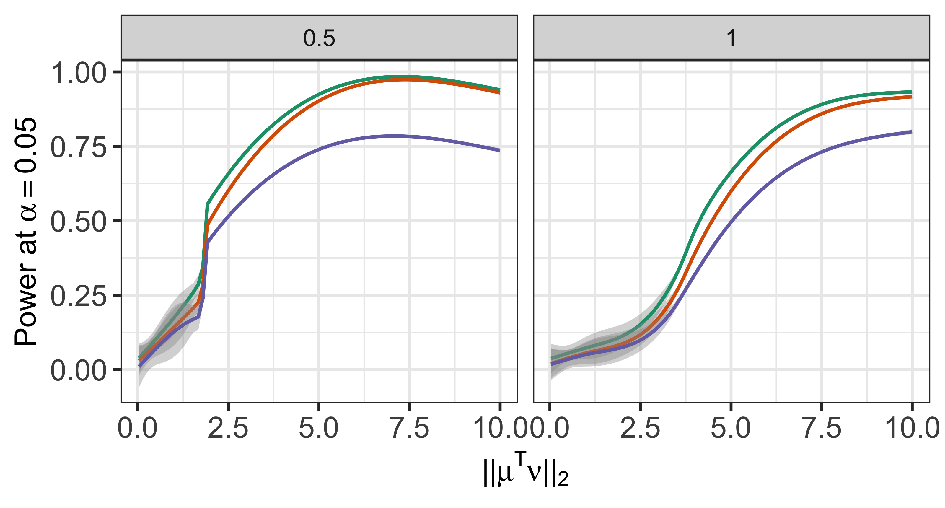
In the first analysis, we consider a different notion of power that does not condition on and being true clusters. In this case, comparing the power of the tests requires a bit of care, because the effect size may differ across simulated datasets from the same data-generating distribution. As a result, we consider the power of the tests as a function of . We fit a regression spline using the gam function in the R package mgcv (Wood, 2017) to obtain a smooth estimate of power on the same simulated datasets from Section \arabicsection.\arabicsubsection. The results are in Figure \arabicfigure. The power of the tests that reject if , , or is less than increases as increases. For a given value of and , the test based on has the highest power, followed by that based on ; the test based on has the lowest power.
In the second analysis, we consider the conditional power (defined in (\arabicequation)) of the tests based on , , and under a different data generating model than (\arabicequation). We generate data from (\arabicequation) with and
| (A.\arabicequation) |
where, is taken to be a multiple of 10, and for , has orthogonal rows, with for . As in Section \arabicsection.\arabicsubsection, we can think of as “true clusters”. Under (A.\arabicequation), the pairwise distance between each pair of true clusters is .
(a) (b)

(c) (d)
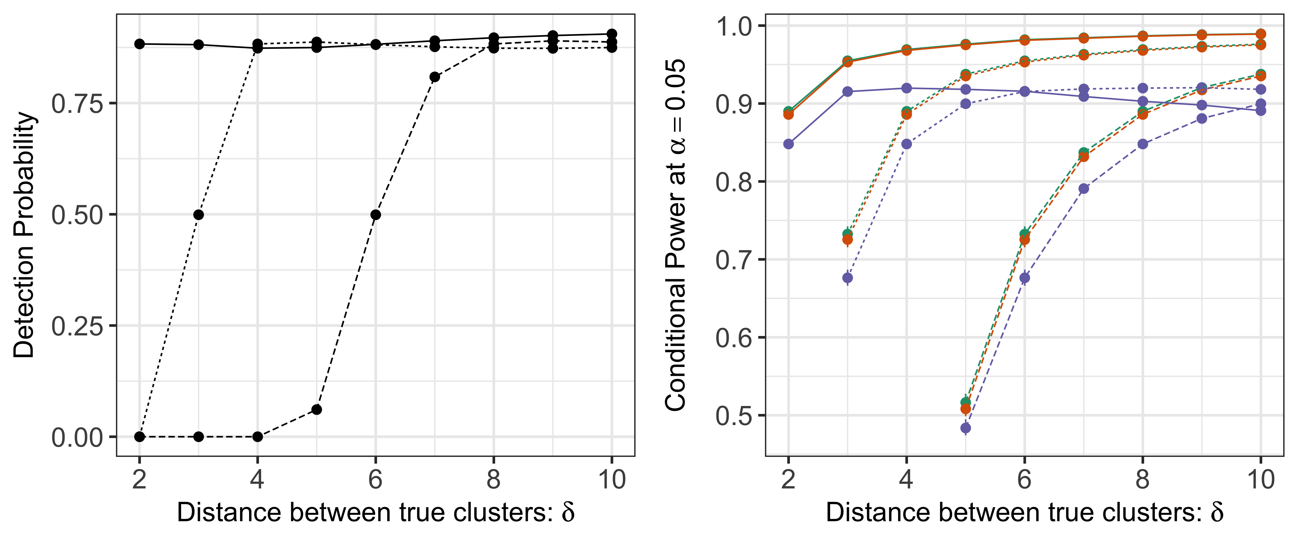
We generate datasets from (A.\arabicequation) with ,, and . For each simulated dataset, we apply -means clustering with and reject if , , or is less than . Figure \arabicfigure(a) displays the detection probability (\arabicequation) of -means clustering as a function of in (A.\arabicequation). Under model (\arabicequation), the detection probability increases as a function of in (A.\arabicequation) across all values of . For a given value of , a larger value of leads to lower detection probability. Figure \arabicfigure(b) displays the conditional power (\arabicequation) for the tests based on , , and . For some combinations of and , the conditional power is not displayed, because the true clusters are never recovered in simulation. For all tests and values of under consideration, conditional power is an increasing function of . For a given test and a value of , smaller leads to higher conditional power. Moreover, for the same values of and , the test based on has the highest conditional power, followed closely by the test based of . Using leads to a less powerful test, especially for larger values of . As a comparison, we included the detection probability and conditional power under model (\arabicequation) with in panels (c) and (d) of Figure \arabicfigure. The tests under consideration behave qualitatively similarly as a function of and . Under (\arabicequation), we observe an even larger gap between the power of the test based on and the power of the test based on .
A.\arabicsubsection Additional results for real data applications
In this section, we visualize the estimated clusters for the single cell RNA-sequencing data in Section \arabicsection.\arabicsubsection.
