Efficient Convex Optimization Requires Superlinear Memory

Abstract

We show that any memory-constrained, first-order algorithm which minimizes $d$-dimensional, $1$-Lipschitz convex functions over the unit ball to $1/\operatorname{\mathrm{poly}}(d)$ accuracy using at most $d^{1.25-\delta}$ bits of memory must make at least $\tilde{\Omega}(d^{1+(4/3)\delta})$ first-order queries (for any constant $\delta\in[0,1/4]$). Consequently, the performance of such memory-constrained algorithms are a polynomial factor worse than the optimal $\tilde{O}(d)$ query bound for this problem obtained by cutting plane methods that use $\tilde{O}(d^{2})$ memory. This resolves a COLT 2019 open problem of Woodworth and Srebro.

1 Introduction

Minimizing a convex objective function $f:\mathbb{R}^{d}\to\mathbb{R}$ given access to a first order oracle—that returns the function evaluation and (sub)gradient $(f(\mathbf{x}),\nabla f(\mathbf{x}))$ when queried for point $\mathbf{x}$—is a canonical problem and fundamental primitive in machine learning and optimization.

There are methods that, given any $1$-Lipschitz, convex $f:\mathbb{R}^{d}\rightarrow\mathbb{R}$ accessible via a first-order oracle, compute an $\epsilon$-approximate minimizer over the unit ball with just $\operatorname{\mathcal{O}}(\min\{\epsilon^{-2},d\log(1/\epsilon)\})$ first order queries. This query complexity is worst-case optimal [47] and foundational in optimization theory. $\operatorname{\mathcal{O}}(\epsilon^{-2})$ queries is achievable using subgradient descent; this is a simple, widely-used, eminently practical method that solves the problem using a total of $\operatorname{\mathcal{O}}(d\epsilon^{-2})$ computation time (assuming arithmetic operations on $\operatorname{\mathcal{O}}(\log(d/\epsilon))$-bit numbers take constant time). On the other hand, building on the $O(d^{2}\log(1/\epsilon))$ query complexity of the well-known ellipsoid method [73, 57], different cutting plane methods achieve a query complexity of $\operatorname{\mathcal{O}}(d\log(1/\epsilon))$, e.g. center of mass with sampling based techniques [37, 14], volumetric center [64, 5], inscribed ellipsoid [36, 44]; these methods are perhaps less frequently used in practice and large-scale learning and all use at least $\Omega(d^{3}\log(1/\epsilon))$-time, even with recent improvements [39, 32].

Though state-of-the-art cutting plane methods have larger computational overhead and are sometimes regarded as impractical in different settings, for small enough $\epsilon$, they give the state-of-the-art query bounds. Further, in different theoretical settings, e.g. semidefinite programming [3, 59, 39], submodular optimization [40, 24, 39, 30] and equilibrium computation [48, 31], cutting-plane-methods have yielded state-of-the-art runtimes at various points of time. This leads to the natural question of what is needed of a method to significantly outperform gradient descent and take advantage of the improved query complexity enjoyed by cutting plane methods? Can we design methods that obtain optimal query complexities while maintaining the practicality of gradient descent methods?

Towards addressing this question, in a COLT 2019 open problem, [70] suggested using memory as a lens. While subgradient descent can be implemented using just $\operatorname{\mathcal{O}}(d\log(1/\epsilon))$-bits of memory [70] all known methods that achieve a query complexity significantly better than gradient descent, e.g. cutting plane methods, require $\Omega(d^{2}\log(1/\epsilon))$ bits of memory. Understanding the trade-offs in memory and query complexity for convex optimization could inform the design of future efficient optimization methods.

In this paper we show that memory does play a critical role in attaining optimal query complexity for convex optimization. Our main result is the following theorem which shows that any algorithm whose memory usage is sufficiently small (though still superlinear) must make polynomially more queries to a first-order oracle than cutting plane methods.

Specifically, any algorithm that uses significantly less than $d^{1.25}$ bits of memory requires a polynomial factor more first order queries than the optimal $\operatorname{\mathcal{O}}(d\log(d))$ queries achieved by quadratic memory cutting plane methods.

Theorem 1.

For some $\epsilon\geq 1/\operatorname{\mathrm{poly}}(d)$ and any $\delta\in[0,\nicefrac{{1}}{{4}}]$ the following is true: any algorithm which is guaranteed to output an $\epsilon$-optimal point with probability at least $\nicefrac{{2}}{{3}}$ given first order oracle access to any $1$-Lipschitz convex function must use either at least $d^{1.25-\delta}$ bits of memory or make $\tilde{\Omega}(d^{1+\frac{4}{3}\delta})$ first order queries (where the $\tilde{\Omega}$ notation hides poly-logarithmic factors in $d$).

Beyond shedding light on the complexity of a fundamental memory-constrained optimization problem, we provide several tools for establishing such lower bounds. In particular, we introduce a set of properties which are sufficient for an optimization problem to exhibit a memory-lower bound and provide an information-theoretic framework to prove these lower bounds. We hope these tools are an aid to future work on the role of memory in optimization.

This work fits within the broader context of understanding fundamental resource tradeoffs for optimization and learning. For many settings, establishing (unconditional) query/time or memory/time tradeoffs is notoriously hard—perhaps akin to P vs NP (e.g. providing time lower bounds for cutting plane methods). Questions of memory/query and memory/data tradeoffs, however, have a more information theoretic nature and hence seem more approachable. Together with the increasing importance of memory considerations in large-scale optimization and learning, there is a strong case for pinning down the landscape of such tradeoffs, which may offer a new perspective on the current suite of algorithms and inform the effort to develop new ones.

1.1 Technical Overview and Contributions

To prove Theorem 1, we provide an explicit distribution over functions that is hard for any memory-constrained randomized algorithm to optimize. Though the proof requires care and we introduce a variety of machinery to obtain it, this lower bounding family of functions is simple to state. The function is a variant of the so-called “Nemirovski” function, which has been used to show lower bounds for highly parallel non-smooth convex optimization [43, 11, 12].

Formally, our difficult class of functions for memory size $M$ is constructed as follows: for some $\gamma>0$ and some $N=\operatorname{\tilde{\mathcal{O}}}\left(d^{2}/M\right)$ let $\mathbf{v}_{1},\ldots,\mathbf{v}_{N}$ be unit vectors drawn i.i.d. from the $d$ dimensional scaled hypercube $\mathbf{v}_{i}\overset{\text{i.i.d.}}{\sim}\mathsf{Unif}\left(d^{-1/2}\mathcal{H}_{d}\right)$ and let $\mathbf{a}_{1},\ldots,\mathbf{a}_{\lfloor d/2\rfloor}$ be drawn i.i.d. from the hypercube, $\mathbf{a}_{j}\sim\mathsf{Unif}\left(\mathcal{H}_{d}\right)$ where $\alpha\mathcal{H}_{d}\coloneqq\left\{\pm\alpha\right\}^{d}$. Let $\mathbf{A}=\left(\mathbf{a}_{1},\dots,\mathbf{a}_{\lfloor d/2\rfloor}\right)$ and define

$$F(\mathbf{x})=(1/d^{6})\max\left\{d^{5}\left\|{\mathbf{A}\mathbf{x}}\right\|_{\infty}-1,\max_{i\in[N]}\mathbf{v}_{i}^{\top}\mathbf{x}-i\gamma\right\}.$$ (1.1)

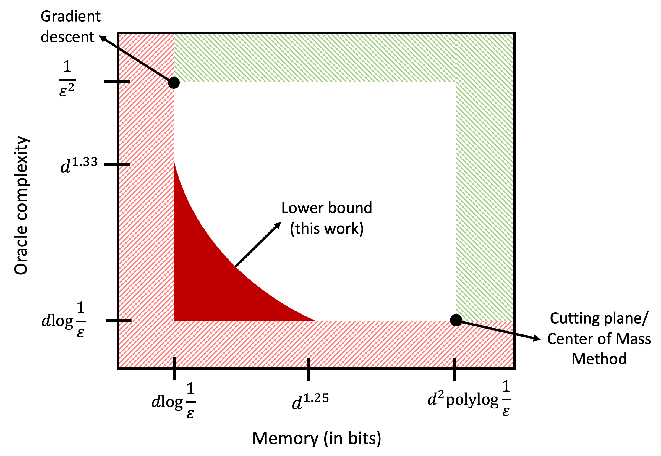
Figure 1: Tradeoffs between available memory and first-order oracle complexity for minimizing 1-Lipschitz convex functions over the unit ball (adapted from [70]). The dashed red “L” shaped region corresponds to information-theoretic lower bounds on the memory and query-complexity. The dashed green inverted “L” shaped region corresponds to known upper bounds. This work shows that the solid red region is not achievable for any algorithm.

Rather than give a direct proof of Theorem 1 using this explicit function we provide a more abstract framework which gives broader insight into which kinds of functions could lead to non-trivial memory-constrained lower bounds, and which might lead to tighter lower bounds in the future. To that end we introduce the notion of a memory-sensitive class which delineates the key properties of a distribution over functions that lead to memory-constrained lower bounds. We show that for such functions, the problem of memory constrained optimization is at least as hard as the following problem of finding a set of vectors which are approximately orthogonal to another set of vectors:

Definition 2 (Informal version of the Orthogonal Vector Game).

Given $\mathbf{A}\in\{\pm 1\}^{d/2\times d}$, the Player’s objective is to return a set of $k$ vectors $\{\mathbf{y}_{1},\dots,\mathbf{y}_{k}\}$ which satisfy

1. $\forall i\in[k],\mathbf{y}_{i}$ is approximately orthogonal to all the rows of $\mathbf{A}:\left\|{\mathbf{A}\mathbf{y}_{i}}\right\|_{\infty}/\left\|{\mathbf{y}_{i}}\right\|_{2}\leq d^{-4}$.

2. The set of vectors $\{\mathbf{y}_{1},\dots,\mathbf{y}_{k}\}$ is robustly linearly independent: denoting $S_{0}=\varnothing,S_{i}=\mathsf{span}(\mathbf{y}_{1},\dots,\mathbf{y}_{i})$, $\mathrm{Proj}_{S_{i-1}}(\mathbf{y}_{i})/\left\|{\mathbf{y}_{i}}\right\|_{2}\leq 1-1/d^{2}$,

where the notation $\mathrm{Proj}_{S}(\mathbf{x})$ denotes the vector in the subspace $S$ which is closest in $\left\|{\cdot}\right\|_{2}$ to $\mathbf{x}$. The game proceeds as follows: The Player first gets to observe $\mathbf{A}$ and store a $M$-bit long $\mathsf{Message}$ about $\mathbf{A}$. She does not subsequently have free access to $\mathbf{A}$, but can adaptively make up to $m$ queries as follows: for $i\in[m]$, based on $\mathsf{Message}$ and all previous queries and their results, she can request any row $i\in[d/2]$ of the matrix $\mathbf{A}$. Finally, she outputs a set of $k$ vectors as a function of $\mathsf{Message}$ and all $m$ queries and their results.

Note that the Player can trivially win the game for $M\geq{\Omega}(dk),m=0$ (by just storing a satisfactory set of $k$ vectors in the $\mathsf{Message}$) and for $M=0,m=d/2$ (by querying all rows of $\mathbf{A}$). We show a lower bound that this is essentially all that is possible: for $\mathbf{A}$ sampled uniformly at random from $\left\{\pm 1\right\}^{d/2\times d}$, if $M$ is a constant factor smaller than $dk$, then the Player must make at least $d/5$ queries to win with probability at least $2/3$. Our analysis proceeds via an intuitive information-theoretic framework, which could have applications for showing query lower bounds for memory-constrained algorithms in other optimization and learning settings. We sketch the analysis in Section 3.2.

1.2 Related Work

Memory-sample tradeoffs for learning

There is a recent line of work to understand learning under information constraints such as limited memory or communication constraints [6, 20, 74, 25, 56, 4, 54, 62, 7, 22, 21, 67]. Most of these results obtain lower bounds for the regime when the available memory is less than that required to store a single datapoint (with the notable exception of [22] and [21]). However the breakthrough paper [50] showed an exponential lower bound on the number of random examples needed for learning parities with memory as large as quadratic. Subsequent work extended and refined this style of result to multiple learning problems over finite fields [41, 9, 42, 35, 51, 26].

Most related to our line of work is [60], which considers the continuous valued learning/optimization problem of performing linear regression given access to randomly drawn examples from an isotropic Gaussian. They show that any sub-quadratic memory algorithm for the problem needs $\Omega(d\log\log(1/\epsilon)))$ samples to find an $\epsilon$-optimal solution for $\epsilon\leq 1/d^{\Omega(\log d)}$, whereas in this regime an algorithm with memory $\tilde{\operatorname{\mathcal{O}}}(d^{2})$ can find an $\epsilon$-optimal solution with only $d$ examples. Since each example provides an unbiased estimate of the expected regression loss, this translates to a lower bound for convex optimization given access to a stochastic gradient oracle. However the upper bound of $d$ examples is not a generic convex optimization algorithm/convergence rate but comes from the fact that the linear systems can be solved to the required accuracy using $d$ examples.

There is also significant work on memory lower bounds for streaming algorithms, e.g. [2, 15, 18, 21], where the setup is that the algorithm only gets a single-pass over a data stream.

Lower bounds for convex optimization

Starting with the early work of [47], there is extensive literature on lower bounds for convex optimization. Some of the key results in this area include classical lower bounds for finding approximate minimizers of Lipschitz functions with access to a subgradient oracle [47, 45, 8], including recent progress on lower bounds for randomized algorithms [68, 69, 55, 58, 10, 63]. There is also work on the effect of parallelism on these lower bounds [43, 12, 19, 11]. For more details, we refer the reader to surveys such as [45] and [13].

Memory-limited optimization algorithms

While the focus of this work is lower bounds, there is a long line of work on developing memory-efficient optimization algorithms, including various techniques that leverage second-order structure via first-order methods such as Limited-memory-BFGS [46, 38] and the conjugate gradient (CG) method for solving linear systems [27] and various non-linear extensions of CG [23, 29] and methods based on subsampling and sketching the Hessian [49, 71, 52]. A related line of work is on communication-efficient optimization algorithms for distributed settings (see [34, 61, 33, 1, 72] and references therein).

2 Setup and Overview of Results

We consider optimization methods for convex, Lipschitz-continuous functions $F:\mathbb{R}^{d}\to\mathbb{R}$ over the unit-ball with access to a first-order oracle. Our goal is to understand how the (oracle) query complexity of algorithms is effected by restrictions on the memory available to the algorithm. Our results apply to a rather general definition of memory constrained first-order algorithms, which includes algorithms that use arbitrarily large memory at query time but can save at most $M$ bits of information in between interactions with the first-order oracle. More formally we have Definition 3.

Definition 3 ($M$-bit memory constrained deterministic algorithm).

An $M$-bit (memory constrained) deterministic algorithm with first-order oracle access, $\mathcal{A}_{\textrm{det}}$, is the iterative execution of a sequence of functions $\left\{\phi_{\textrm{query},t},\phi_{\textrm{update},t}\right\}_{t\geq 1}$, where $t$ denotes the iteration number. The function $\phi_{\textrm{query},t}$ maps the ${(t-1)}^{\textrm{th}}$ memory state of size at most $M$ bits to the ${t}^{\textrm{th}}$ query vector, $\phi_{\textrm{query},t}(\mathsf{Memory}_{t-1})=\mathbf{x}_{t}$. The algorithm is allowed to use an arbitrarily large amount of memory to execute $\phi_{\textrm{query},t}$. Upon querying $\mathbf{x}_{t}$, some first order oracle returns $F(\mathbf{x}_{t})$ and a subgradient $\mathbf{g}_{\mathbf{x}_{t}}\in\partial F(\mathbf{x}_{t})$. The second function maps the first order information and the old memory state to a new memory state of at most $M$ bits, $\mathsf{Memory}_{t}=\phi_{\textrm{update},t}\left(\mathbf{x}_{t},F(\mathbf{x}_{t}),\mathbf{g}_{\mathbf{x}_{t}},\mathsf{Memory}_{t-1}\right)$. Again, the algorithm may use unlimited memory to execute $\phi_{\textrm{update},t}$.

Note that our definition of a memory constrained algorithm is equivalent to the definition given by [70]. Our analysis also allows for randomized algorithms which will often be denoted as $\mathcal{A}_{\textrm{rand}}$.

Definition 4 ($M$-bit memory constrained randomized algorithm).

An $M$-bit (memory constrained) randomized algorithm with first-order oracle access, $\mathcal{A}_{\textrm{rand}}$, is a deterministic algorithm with access to a string $R$ of uniformly random bits which has length $2^{d}$.

In what follows we use the notation $\mathcal{O}_{F}(\mathbf{x})$ to denote the first-order oracle which, when queried at some vector $\mathbf{x}$, returns the pair $(F(\mathbf{x}),\mathbf{g}_{\mathbf{x}})$ where $\mathbf{g}_{\mathbf{x}}\in\partial F(\mathbf{x})$ is a subgradient of $F$ at $\mathbf{x}$. We will also refer to a sub-gradient oracle and use the overloaded notation $\mathbf{g}_{F}(\mathbf{x})$ to denote the oracle which simply returns $\mathbf{g}_{\mathbf{x}}$. It will be useful to refer to the specific sequence of vectors $\mathbf{x}$ queried by some algorithm $\mathcal{A}$ paired with the subgradient $\mathbf{g}$ returned by the oracle.

Definition 5 (Query sequence).

Given an algorithm $\mathcal{A}$ with access to some first-order oracle $\mathcal{O}$ we let $\mathsf{Seq}(\mathcal{A},\mathcal{O})=\left\{(\mathbf{x}_{i},\mathbf{g}_{i})\right\}_{i}$ denote the query sequence of vectors $\mathbf{x}_{i}$ queried by the algorithm paired with the subgradient $\mathbf{g}_{i}$ returned by the oracle $\mathcal{O}$.

2.1 Proof Strategy

We describe a broad family of optimization problems which may be sensitive to memory constraints. As suggested by the Orthogonal Vector Game (Definition 2), the primitive we leverage is that finding vectors orthogonal to the rows of a given matrix requires either large memory or many queries to observe the rows of the matrix. With that intuition in mind, let $f:\mathbb{R}^{d}\to\mathbb{R}$ be a convex function, let $\mathbf{A}\in\mathbb{R}^{n\times d}$, let $\eta$ be a scaling parameter, and let $\rho$ be a shift parameter; define $F_{f,\mathbf{A},\eta,\rho}(\mathbf{x})$ as the maximum of $f(\mathbf{x})$ and $\eta\left\|{\mathbf{A}\mathbf{x}}\right\|_{\infty}-\rho$:

$$F_{f,\mathbf{A},\eta,\rho}(\mathbf{x})\coloneqq\max\left\{f(\mathbf{x}),\eta\left\|{\mathbf{A}\mathbf{x}}\right\|_{\infty}-\rho\right\}.$$ (2.1)

We often drop the dependence of $\eta$ and $\rho$ and write $F_{f,\mathbf{A},\eta,\rho}$ simply as $F_{f,\mathbf{A}}$. Intuitively, for large enough scaling $\eta$ and appropriate shift $\rho$, minimizing the function $F_{f,\mathbf{A}}(\mathbf{x})$ requires minimizing $f(\mathbf{x})$ in the null space of the matrix $\mathbf{A}$. Any algorithm which uses memory $\Omega(d^{2})$ can learn and store $\mathbf{A}$ in $\operatorname{\mathcal{O}}(d)$ queries so that all future queries are sufficiently orthogonal to $\mathbf{A}$; thus this memory rich algorithm can achieve the information-theoretic lower bound for minimizing $f(\mathbf{x})$ roughly constrained to the nullspace of $\mathbf{A}$.

However, if $\mathbf{A}$ is a random matrix with sufficiently large entropy then $\mathbf{A}$ cannot be compressed to fewer than $\Omega(nd)$ bits. Thus, for $n=\Omega(d)$, an algorithm which uses only memory $o(d^{2-\delta})$ bits for some constant $0<\delta\leq 1$ cannot remember all the information about $\mathbf{A}$. Suppose the function $f$ is such that in order to continue to observe informative subgradients (which we will define formally later in Definition 8), it is not sufficient to submit queries that belong to some small dimensional subspace of the null space of $\mathbf{A}$. Then a memory constrained algorithm must re-learn enough information about $\mathbf{A}$ in order to find a vector in the null space of $\mathbf{A}$ and make a query which returns an informative subgradient for $f$.

2.2 Proof Components

In summary of Section 2.1, there are two critical features of $F_{f,\mathbf{A}}$ which lead to a difficult optimization problem for memory constrained algorithms. First, the distribution underlying random instances of $\mathbf{A}$ must ensure that $\mathbf{A}$ cannot be compressed. Second, the function $f$ must be such that queries which belong to a small dimensional subspace cannot return too many informative subgradients. We formalize these features by defining a memory-sensitive base and a memory-sensitive class. We show that if $\mathbf{A}$ is drawn uniformly at random from a memory-sensitive base and if $f$ and a corresponding first-order oracle are drawn according to a memory-sensitive class then the resulting distribution over $F_{f,\mathbf{A}}(\mathbf{x})$ and its first order oracle provides a difficult instance for memory constrained algorithms to optimize.

Definition 6 ($(k$, $c_{B}$)-memory-sensitive base).

Consider a sequence of sets $\left\{B_{d}\right\}_{d>0}$ where $B_{d}\subset\mathbb{R}^{d}$. We say $\left\{B_{d}\right\}$ is a $(k$, $c_{B}$)-memory-sensitive base if for any $d$, $\left|B_{d}\right|<\infty$ and for $\mathbf{h}\sim\mathsf{Unif}(B_{d})$ the following hold: for any $t\in(0,1/2]$ and any matrix $\mathbf{Z}=\left(\mathbf{z}_{1},\dots,\mathbf{z}_{k}\right)\in\mathbb{R}^{d\times k}$ with orthonormal columns,

$$\mathbb{P}\left(\left\|{\mathbf{h}}\right\|_{2}>d\right)\leq 2^{-d}\qquad\textrm{and}\qquad\mathbb{P}\left(\left\|{\mathbf{Z}^{\top}\mathbf{h}}\right\|_{\infty}\leq t\right)\leq 2^{-c_{B}k}.$$ (2.2)

We write $\mathbf{A}\sim\mathsf{Unif}(B_{d}^{n})$ to mean we draw $\mathbf{a}_{i}\sim\mathsf{Unif}(B_{d})$ and set $\mathbf{A}=\left(\mathbf{a}_{1},\dots,\mathbf{a}_{n}\right)^{\top}$. Theorem 6 shows that the sequence of hypercubes is a memory-sensitive base, proven in Section 4. theoremhypercube Recall that $\mathcal{H}_{d}=\left\{\pm 1\right\}^{d}$ denotes the hypercube. The sequence $\left\{\mathcal{H}_{d}\right\}_{d=d_{0}}^{\infty}$ is a $(k,c_{\mathcal{H}})$ memory-sensitive base for all $k\in[d]$ with some absolute constant $c_{\mathcal{H}}>0$. Next we consider distributions over functions $f$ paired with some subgradient oracle $\mathbf{g}_{f}$. Given $f$ and some $\mathbf{A}\sim\mathsf{Unif}(B_{d}^{n})$ we consider minimizing $F_{f,\mathbf{A}}$ as in Eq. 2.1 with access to an induced first-order oracle:

Definition 7 (Induced First-Order Oracle $\mathcal{O}_{F_{f,\mathbf{A}}}$).

Given a subgradient oracle for $f$, $\mathbf{g}_{f}:\mathbb{R}^{d}\to\mathbb{R}^{d}$, matrix $\mathbf{A}\in\mathbb{R}^{n\times d}$, and parameters $\eta$ and $\rho$, let

$$\mathbf{g}_{\mathbf{A}}(\mathbf{x})\coloneqq\mathbf{a}_{i_{\min}},\textrm{ where }i_{\min}\coloneqq\min\left\{i\in[n]\textrm{ s.t. }\mathbf{a}_{i}^{\top}\mathbf{x}=\left\|{\mathbf{A}\mathbf{x}}\right\|_{\infty}\right\},$$

$$\mathbf{g}_{F_{f,\mathbf{A}}}(\mathbf{x})\coloneqq\begin{cases}&\mathbf{g}_{\mathbf{A}}(\mathbf{x}),\textrm{ if }\eta\left\|{\mathbf{A}\mathbf{x}}\right\|_{\infty}-\rho\geq f(\mathbf{x}),\\ &\mathbf{g}_{f}(\mathbf{x}),\textrm{ else.}\end{cases}$$

The induced first-order oracle for $F_{f,\mathbf{A}}(\mathbf{x})$, denoted as $\mathcal{O}_{F_{f,\mathbf{A}}}$ returns the pair $(F_{f,\mathbf{A}}(\mathbf{x}),\mathbf{g}_{F_{f,\mathbf{A}}}(\mathbf{x}))$.

We also define informative subgradients, formalizing the intuition described at the beginning of this section.

Definition 8 (Informative subgradients).

Given a query sequence $\mathsf{Seq}(\mathcal{A},\mathcal{O}_{F_{f,\mathbf{A}}})=\left\{(\mathbf{x}_{i},\mathbf{g}_{i})\right\}_{i=1}^{T}$ we construct the sub-sequence of informative subgradients as follows: proceed from $i=1,\dots,T$ and include the pair $(\mathbf{x}_{i},\mathbf{g}_{i})$ if and only if $1)$ $f(\mathbf{x}_{i})>\eta\left\|{\mathbf{A}\mathbf{x}_{i}}\right\|_{\infty}-\rho$ and $2)$ no pair $(\mathbf{x},\mathbf{g})$ such that $\mathbf{g}=\mathbf{g}_{i}$ has been selected in the sub-sequence so far. If $(\mathbf{x}_{i},\mathbf{g}_{i})$ is the ${j}^{\textrm{th}}$ pair included in the sub-sequence define $t_{j}=i$ and we call $\mathbf{x}_{i}$ the ${j}^{\textrm{th}}$ informative query and $\mathbf{g}_{i}$ the ${j}^{\textrm{th}}$ informative subgradient.

We can now proceed to the definition of a $(L,M,N,\epsilon{{}^{\star}})$-memory-sensitive class.

Definition 9 ($(L,N,k,\epsilon{{}^{\star}})$-memory-sensitive class).

Let $\mathcal{F}$ be a distribution over functions $f:\mathbb{R}^{d}\to\mathbb{R}$ paired with a valid subgradient oracle $\mathbf{g}_{f}:\mathbb{R}^{d}\to\mathbb{R}^{d}$. For Lipschitz constant $L$, “depth” $N$, “round-length” $k$, and optimality threshold $\epsilon{{}^{\star}}$, we call $\mathcal{F}$ a $(L,N,k,\epsilon{{}^{\star}})$-memory-sensitive class if one can sample from $\mathcal{F}$ with at most $2^{d}$ uniformly random bits, and there exists a choice of $\eta$ and $\rho$ (from Eq. 2.1) such that for any $\mathbf{A}\in\mathbb{R}^{n\times d}$ with rows bounded in $\ell_{2}$-norm by $d$ and any (potentially randomized) unbounded-memory algorithm $\mathcal{A}_{\textrm{rand}}$ which makes at most $Nd$ queries: if $(f,\mathbf{g}_{f})\sim\mathcal{F}$ then with probability at least $\nicefrac{{2}}{{3}}$ (over the randomness in $(f,\mathbf{g}_{f})$ and $\mathcal{A}_{\textrm{rand}}$) the following hold simultaneously:

1. Regularity: $F_{f,\mathbf{A},\eta,\rho}$ is convex and $L$-Lipschitz.

2. Robust independence of informative queries: If $\left\{\mathbf{x}_{t_{j}}\right\}$ is the sequence of informative queries generated by $\mathcal{A}_{\textrm{rand}}$ (as per Definition 8) and $S_{j}\coloneqq\mathsf{span}\left(\{\mathbf{x}_{t_{i}}:\max(1,j-k)\leq i\leq j\}\right)$ then $\forall j\in[N]$

   $$\left\|{\mathrm{Proj}_{S_{j-1}}({\mathbf{x}}_{t_{j}})}\right\|_{2}/\left\|{{\mathbf{x}}_{t_{j}}}\right\|_{2}\leq 1-1/d^{2}.$$ (2.3)

3. Approximate orthogonality: Any query $\mathbf{x}$ with $F_{f,\mathbf{A},\eta,\rho}(\mathbf{x})\neq\eta\left\|{\mathbf{A}\mathbf{x}}\right\|_{\infty}-\rho$ satisfies

   $$\mathbf{g}_{F_{f,\mathbf{A}}}(\mathbf{x})=\mathbf{v}_{1}\textrm{ or }\left\|{\mathbf{A}\mathbf{x}}\right\|_{\infty}/\left\|{\mathbf{x}}\right\|_{2}\leq d^{-4}.$$ (2.4)

4. Necessity of informative subgradients: If $r<N$ then for any $i\leq t_{r}$ (where $t_{r}$ is as in Definition 8),

   $$F_{f,\mathbf{A}}(\mathbf{x}_{i})-F_{f,\mathbf{A}}(\mathbf{x}^{\star})\geq\epsilon{{}^{\star}}.$$ (2.5)

Informally, the robust independence of informative queries condition ensures that any informative query is robustly linearly independent with respect to the previous $k$ informative queries. The approximate orthogonality condition ensures that any query $\mathbf{x}$ which reveals a gradient from $f$ which is not $\mathbf{v}_{1}$ is approximately orthogonal to the rows of $\mathbf{A}$. Finally, the necessity of informative subgradients condition ensures that any algorithm which has queried only $r<N$ informative subgradients from $f$ must have optimality gap greater than $\epsilon{{}^{\star}}$.

The following construction, discussed in the introduction, is a concrete instance of a $(d^{6},N,\lceil 20M/(cd)\rceil,$ $1/(20\sqrt{N}))$-memory-sensitive class with $N\approx(d^{2}/M)^{1/3}$. Theorem 11 proves that the construction is memory sensitive, and the proof appears in Section 4.

Definition 10 (Nemirovski class).

For a given $\gamma>0$ and for $i\in[N]$ draw $\mathbf{v}_{i}\overset{\text{i.i.d.}}{\sim}\mathsf{Unif}\left(d^{-1/2}\mathcal{H}_{d}\right)$ and set

$$f(\mathbf{x})\coloneqq\max_{i\in[N]}\mathbf{v}_{i}^{\top}\mathbf{x}-i\gamma\qquad\textrm{ and }\qquad\mathbf{g}_{f}(\mathbf{x})=\mathbf{v}_{i_{\min}},$$ (2.6)

where $i_{\min}\coloneqq\min\left\{i\in[N]\textrm{ s.t. }\mathbf{v}_{i}^{\top}\mathbf{x}-i\gamma=f(\mathbf{x})\right\}$. Let $\mathcal{N}_{N,\gamma}$ be the distribution of $(f,\mathbf{g}_{f})$, and for a fixed matrix $\mathbf{A}$ let $\mathcal{N}_{N,\gamma,\mathbf{A}}$ be the distribution of the induced first order oracle from Definition 7.

Theorem 11.

For large enough dimension $d$ there is an absolute constant $c>0$ such that for any given $k$, the Nemirovski function class with $\gamma=(400k\log(d)/d)^{1/2}$, $L=d^{6}$, $N=c(d/(k\log d))^{1/3}$, and $\epsilon{{}^{\star}}=1/(20\sqrt{N})$ is a $(L,N,k,\epsilon{{}^{\star}})$-memory-sensitive class.

2.3 Main Results

With the definitions from the previous section in place we may now state our main technical theorem for proving lower bounds on memory constrained optimization.

Theorem 12 (From memory-sensitivity to lower bounds).

For $d\in\mathbb{Z}_{>0}$, memory constraint $M\geq d$, and $\epsilon\in\mathbb{R}_{>0}$, let $\left\{B_{d}\right\}_{d>0}$ be a $(k,c_{B})$-memory-sensitive base and let $\mathcal{F}$ be a $(L,N,k,\epsilon)$-memory-sensitive class  where

$$k=\lceil 20M/(c_{B}d)\rceil\quad\text{ , }\quad N=1/(20\epsilon)^{2}\quad\text{ , and }\quad\epsilon\leq L/(4\sqrt{d})\,.$$ (2.7)

Further, let $\mathbf{A}\sim\mathsf{Unif}(B_{d}^{n})$, let $(f,\mathbf{g}_{f})\sim\mathcal{F}$, and consider $F_{f,\mathbf{A}}$ with oracle $\mathcal{O}_{F_{f,\mathbf{A}}}$ as in Definition 7. Any $M$-bit (potentially) randomized algorithm (as per Definition 4) which outputs an $\epsilon$-optimal point for $F_{f,\mathbf{A}}$ with probability at least $\nicefrac{{2}}{{3}}$ requires at least $c_{B}d^{2}/(10^{6}\epsilon^{2}M)=\Omega(c_{B}d^{2}N/M)$ first-order oracle queries.

Note that by [70], the center of mass algorithm can output an $\epsilon$-optimal point for any $L$-Lipschitz function using $\operatorname{\mathcal{O}}\left(d^{2}\log^{2}\left(LB/\epsilon\right)\right)$ bits of memory and $\operatorname{\mathcal{O}}\left(d\log(LB/\epsilon)\right)$ first-order oracle queries. Comparing this with the lower bound from Theorem 12 we see that for a given $\epsilon\leq\sqrt{L/d}$ if there exists a $(L,1/(20\epsilon)^{2},k,\epsilon)$ memory-sensitive class, then $M$-bit algorithms become unable to achieve the optimal quadratic memory query complexity once the memory is smaller than $o\left(d/(\epsilon^{2}\log(LB/\epsilon)\right)$ many bits. Further, Theorem 12 yields a natural approach for obtaining improved lower bounds. If one exhibits a memory-sensitive class with depth $N=d$, then Theorem 12 would imply that any algorithm using memory of size at most $M=d^{2-\delta}$ requires at least $\Omega\left(d^{1+\delta}\right)$ many first-order oracle queries in order to output an $\epsilon$-optimal point.

Given Definitions 6, 11 and 12, the proof of Theorem 1 follows by setting the various parameters.

Proof of Theorem 1.

Consider $M$-bit memory constrained (potentially) randomized algorithms (as per Definition 4) where $M$ can be written in the form $d^{1.25-\delta}$ for some $\delta\in[0,\nicefrac{{1}}{{4}}]$. By Theorem 11, for some absolute constant $c>0$ and for $d$ large enough and any given $k$, if $\gamma=\sqrt{400k\log d/d}$, $N=c(d/(k\log d))^{1/3}$, and $\epsilon=1/(20d^{6}\sqrt{N})$, the Nemirovski function class from Definition 10 is $(1,N,k,\epsilon)$-memory-sensitive (where we rescaled by the Lipschitz constant $1/d^{6}$). Set $k=\lceil 20M/(c_{\mathcal{H}}d)\rceil$ (where $c_{\mathcal{H}}$ is as in Definition 6). Let $(f,\mathbf{g}_{f})\sim\mathcal{N}_{\gamma,N}$ and $\mathbf{A}\sim\mathsf{Unif}\left(\mathcal{H}_{d}^{n}\right)$ and suppose $\mathcal{A}_{\textrm{rand}}$ is an $M$-bit algorithm which outputs an $\epsilon$-optimal point for $F_{f,\mathbf{A}}$ with failure probability at most $\nicefrac{{1}}{{3}}$. By Theorem 12, $\mathcal{A}_{\textrm{rand}}$ requires at least $c_{\mathcal{H}}Nd^{2}/M\geq c\left(d^{2}/M\right)^{4/3}(1/\log^{1/3}d)$ many queries. Recalling that $M=d^{1.25-\delta}$ for $\delta\in[0,\nicefrac{{1}}{{4}}]$ results in a lower bound of $\tilde{\Omega}(d^{1+\frac{4}{3}\delta})$ many queries. ∎

Why $d^{4/3}$: Parameter tradeoffs in our lower bound.

An idealized lower bound in this setting would arise from exhibiting an $f$ such that to obtain any informative gradient requires $\Theta(d)$ more queries to re-learn $\mathbf{A}$ and in order to optimize $f$ we need to observe at least $\Omega(d)$ such informative gradients. Our proof deviates from this ideal on both fronts. We do prove that we need $\Theta(d)$ queries to get any informative gradients, though with this number we cannot preclude getting $M/d$ informative gradients. Second, our Nemirovski function can be optimized while learning only $O((d^{2}/M)^{1/3})$-informative gradients (there are modifications to Nemirovski that increase this number [11], though for those functions, informative gradients can be observed while working within a small subspace). For our analysis we have, very roughly, that $\Omega(d)$ queries are needed to observe $M/d$ informative gradients and we must observe $(d^{2}/M)^{1/3}$ informative gradients to optimize the Nemirovski function. Therefore optimizing the Nemirovksi function requires $\Omega\left(d\right)\times\frac{(d^{2}/M)^{1/3}}{M/d}=(d^{2}/M)^{4/3}$ many queries; and so when $M=O(d)$ we have a lower bound of $d^{4/3}$ queries.

3 Proof Overview

Here we give the proof of Theorem 12. In Section 3.1 we present our first key idea, which relates the optimization problem in (2.1) to the Orthogonal Vector Game (which was introduced informally in Definition 2). Next, in Section 3.2, we show that winning this Orthogonal Vector Game is difficult with memory constraints.

3.1 The Orthogonal Vector Game

We formally define the Orthogonal Vector Game in Game 1 and then relate it to minimizing $F_{f,\mathbf{A}}$ (Eq. 2.1).

Input : $d,k,m,B_{d},M$

1 Oracle: For $n\leftarrow d/2$, sample $\mathbf{A}\sim\mathsf{Unif}(B_{d}^{n})$.

2 Oracle: Sample a string $R$ of uniformly random bits of length $3\cdot 2^{d}$ (the Player has read-only access to $R$ throughout the game).

3 Player: Observe $\mathbf{A}$ and $R$, and store a $M$-bit message, $\mathsf{Message}$, about the matrix $\mathbf{A}$.

4

5for $i\in[m]$ do

6       Player: Based on $\mathsf{Message}$, $R$, and any previous queries and responses, use a deterministic algorithm to submit a query $\mathbf{x}_{i}\in\mathbb{R}^{d}$.

7       Oracle: As the response to query $\mathbf{x}_{i}$, return $\mathbf{g}_{i}=\mathbf{g}_{\mathbf{A}}(\mathbf{x}_{i})$ (see Definition 7).

8      

9Player: Let $\mathbf{X}$ and $\mathbf{G}$ be matrices with queries $\{\mathbf{x}_{i},i\in[m]\}$ and responses $\{\mathbf{g}_{i},i\in[m]\}$ as rows, respectively. Based on $(\mathbf{X},\mathbf{G},\mathsf{Message},R)$, use a deterministic function to return vectors $\{\mathbf{y}_{1},\dots,\mathbf{y}_{k}\}$ to the Oracle. Let $\mathbf{Y}$ be the matrix with these vectors as rows.

10 The Player wins if the returned vectors are successful, where a vector $\mathbf{y}_{i}$ is successful if $(1)\left\|{\mathbf{A}\mathbf{y}_{i}}\right\|_{\infty}/\left\|{\mathbf{y}_{i}}\right\|_{2}\leq d^{-4}$, and $(2)\text{ }\mathrm{Proj}_{S_{i-1}}(\mathbf{y}_{i})/\left\|{\mathbf{y}_{i}}\right\|_{2}\leq 1-1/d^{2}\text{ where }S_{0}\coloneqq\varnothing\text{, and }S_{i}\coloneqq\mathsf{span}(\mathbf{y}_{1},\dots,\mathbf{y}_{i})$.

Game 1 Orthogonal Vector Game

Lemma 13 (Optimizing $F_{f,\mathbf{A}}$ is harder than winning the Orthogonal Vector Game).

Let $\mathbf{A}\sim\mathsf{Unif}(B_{d}^{n})$ and $(f,\mathbf{g}_{f})\sim\mathcal{F}$, where $\left\{B_{d}\right\}_{d>0}$ is a $(k,c_{B})$-memory-sensitive base and $\mathcal{F}$ is a $(L,N,k,\epsilon{{}^{\star}})$ memory-sensitive class. If there exists an $M$-bit algorithm with first-order oracle access that outputs an $\epsilon{{}^{\star}}$-optimal point for minimizing $F_{f,\mathbf{A}}$ using $m\lfloor N/(k+1)\rfloor$ queries with probability at least $\nicefrac{{2}}{{3}}$ over the randomness in the algorithm and choice of $f$ and $\mathbf{A}$, then the Player can win the Orthogonal Vector Game with probability at least $\nicefrac{{1}}{{3}}$ over the randomness in the Player’s strategy and $\mathbf{A}$.

Lemma 13 serves as a bridge between the optimization problem of minimizing $F_{f,\mathbf{A}}$ and the Orthogonal Vector Game. Here we provide a brief proof sketch before the detailed proof: Let $\mathcal{A}_{\textrm{rand}}$ denote a hypothetical $M$-bit memory algorithm for optimizing $F_{f,\mathbf{A}}$ (Definition 4). The Player samples a random function/oracle pair $(f,\mathbf{g}_{f})$ from the memory-sensitive class $\mathcal{F}$. Then, she uses $\mathcal{A}_{\textrm{rand}}$ to optimize $F_{f,\mathbf{A}}$, and issues queries that $\mathcal{A}_{\textrm{rand}}$ makes to the oracle in the Orthogonal Vector Game. Notice that with access to $\mathbf{g}_{f}(\mathbf{x})$ and the oracle’s response $\mathbf{g}_{\mathbf{A}}(\mathbf{x})$, she can implement the sub-gradient oracle $\mathbf{g}_{F_{f,\mathbf{A}}}$ (Definition 7). We then use the memory-sensitive properties of $f$ to argue that informative queries made by $\mathcal{A}_{\textrm{rand}}$ must also be successful queries in the Orthogonal Vector Game, and that $\mathcal{A}_{\textrm{rand}}$ must make enough informative queries to find an $\epsilon{{}^{\star}}$-optimal point.

Proof of Lemma 13.

In Algorithm 2 we provide a strategy for the Player which uses $\mathcal{A}_{\textrm{rand}}$ (the $M$-bit algorithm that minimizes $F_{f,\mathbf{A}}$) to win the Orthogonal Vector Gamewith probability at least 1/3 over the randomness in $R$ and $\mathbf{A}$.

Input : $d,m,\mathcal{A}_{\textrm{rand}},\mathcal{F},R$

1 Part 1, Strategy to store $\mathsf{Message}$ using $\mathbf{A}$:

2      

3      Divide random string $R$ into three equal parts $R_{1},R_{2},R_{3}$, each of length $2^{d}$

4       Sample a function/oracle pair $(f,\mathbf{g}_{f})\sim\mathcal{F}$ (using $R_{1}$ to supply the required random bits)

5       for $i\in\{1,\ldots,\lfloor N/(k+1)\rfloor\}$ do

6             Run $\mathcal{A}_{\textrm{rand}}$ to minimize $F_{f,\mathbf{A}}$ until $i(k+1)$ informative subgradients are observed from $f$, using $R_{2}$ to supply any random bits for the execution of $\mathcal{A}_{\textrm{rand}}$. Let $\mathsf{Memory}_{i}$ be $\mathcal{A}_{\textrm{rand}}$’s memory state at the end of this step.

7             Continue running $\mathcal{A}_{\textrm{rand}}$ to minimize $F_{f,\mathbf{A}}$ until $(k+1)$ more informative subgradients are observed from $f$, now using $R_{3}$ to supply any random bits. Let $t$ be the total number of first-order queries made by the algorithm in this step.

8             if $t\leq m$ then

9                   return $\mathsf{Memory}_{i}$ as the $\mathsf{Message}$ to be stored

10                  

11      return Failure

12 Part 2, Strategy to make queries:

13       Use $R_{1}$ to resample the function/oracle pair $(f,\mathbf{g}_{f})$

14       Set $\mathcal{A}_{\textrm{rand}}$’s memory state to be $\mathsf{Message}$.

15       for $i\in[m]$, do

16             Run $\mathcal{A}_{\textrm{rand}}$ to issue query $\mathbf{x}_{i}$ to minimize $F_{f,\mathbf{A}}(\mathbf{x})$ (using $R_{3}$ to supply any random bits)

17             Submit query $\mathbf{x}_{i}$ to Oracle in the Orthogonal Vector Game, to get response $\mathbf{g}_{i}$

18             Simulation of first-order oracle $\mathcal{O}_{F_{f,\mathbf{A}}}$:

19                   $F_{f,\mathbf{A}}(\mathbf{x}_{i})=\max(\eta|\mathbf{g}_{i}^{\top}\mathbf{x}_{i}|-\rho,f(\mathbf{x}_{i}))$

20                   if $F_{f,\mathbf{A}}(\mathbf{x}_{i})\geq f(\mathbf{x}_{i})$ then  $\mathbf{g}_{F_{f,\mathbf{A}}}(\mathbf{x}_{i})=\mathbf{g}_{i}$

21                   else  $\mathbf{g}_{F_{f,\mathbf{A}}}(\mathbf{x}_{i})=\mathbf{g}_{f}(\mathbf{x}_{i})$

22                  

23            Pass $(F_{f,\mathbf{A}}(\mathbf{x}_{i}),\mathbf{g}_{F_{f,\mathbf{A}}}(\mathbf{x}_{i}))$ to $\mathcal{A}_{\textrm{rand}}$ to update its state

24            

25 Part 3, Strategy to find successful vectors based on $(\mathbf{X},\mathbf{G},\mathsf{Message},R)$:

26       for every subset $\{\mathbf{x}_{m_{1}},\dots,\mathbf{x}_{m_{k}}\}$ of the queries $\{\mathbf{x}_{1},\dots,\mathbf{x}_{m}\}$ do

27             Check if $|\mathbf{g}_{m_{j}}^{\top}\mathbf{x}_{m_{j}}|/\left\|{\mathbf{x}_{m_{j}}}\right\|\leq d^{-4}\;\forall j\in[k]$

28             Check if $\{\mathbf{x}_{m_{1}},\dots,\mathbf{x}_{m_{k}}\}$ are robustly linearly independent (as in Definition 9)

29             if the above two conditions are satisfied then

30                   return $\{\mathbf{x}_{m_{1}},\dots,\mathbf{x}_{m_{k}}\}$ to the Oracle

31      return Failure

Algorithm 2 Player’s strategy for the Orthogonal Vector Game

The Player uses the random string $R$ to sample a function/oracle pair $(f,\mathbf{g}_{f})\sim\mathcal{F}$, and to run the algorithm $\mathcal{A}_{\textrm{rand}}$ (if it is randomized). The first part $R_{1}$ of the random string is used to sample $(f,\mathbf{g}_{f})\sim\mathcal{F}$. Note that by Definition 9, $f$ and $\mathbf{g}_{f}$ can be sampled from $\mathcal{F}$ with at most $2^{d}$ random bits, therefore the Player can sample $(f,\mathbf{g}_{f})\sim\mathcal{F}$ using $R_{1}$. The second and third parts of $R$ ($R_{2}$ and $R_{3}$) are used to supply any random bits for the execution of $\mathcal{A}_{\textrm{rand}}$. We note that by Definition 4 a randomized algorithm uses at most $2^{d}$ random bits, therefore the Player will not run out of random bits to supply $\mathcal{A}_{\textrm{rand}}$.

Let $G$ be the event that $R_{1},R_{2},R_{3}$, and $\mathbf{A}$ have the property that (1) $\mathcal{A}_{\textrm{rand}}$ succeeds in finding an $\epsilon^{\star}$-optimal point for the function $F_{f,\mathbf{A}}(\mathbf{x})$, and (2) all the properties of a memory-sensitive class in Definition 9 are satisfied. By the guarantee in Lemma 13, $\mathcal{A}_{\textrm{rand}}$ has the property that it finds an $\epsilon^{\star}$-optimal point with failure probability at most $\nicefrac{{1}}{{3}}$ over the randomness in $\mathbf{A}$, $R_{1}$ (the randomness in $(f,\mathbf{g}_{f})$) and $R_{2},R_{3}$ (the internal randomness used by $\mathcal{A}_{\textrm{rand}}$). Also, the properties in Definition 9 are satisfied with failure probability at most $\nicefrac{{1}}{{3}}$ by definition. Therefore, by a union bound, $\Pr[G]\geq\nicefrac{{1}}{{3}}$. We will condition on $G$ for the rest of the proof.

We now analyze Part 1 of the Player’s strategy, which involves deciding on the $M$-bit $\mathsf{Message}$ to store. We begin by noting that since $\mathcal{A}_{\textrm{rand}}$ runs with $M$ memory, the stored $\mathsf{Message}$ is at most $M$ bits long. We now prove that Part 1 does not fail under the event $G$.

Recall the definition of informative subgradients from Definition 8, and note that by Eq. 2.5 in Definition 9, under event $G$ if $\mathcal{A}_{\textrm{rand}}$ finds an $\epsilon^{\star}$-optimal point, then $\mathcal{A}_{\textrm{rand}}$ must observe at least $N$ informative subgradients from $f$. Therefore, under event $G$, since $\mathcal{A}_{\textrm{rand}}$ can find an $\epsilon^{\star}$-optimal point using $m\lfloor N/(k+1)\rfloor$ queries it can observe $N$ informative subgradients from $f$ using $m\lfloor N/(k+1)\rfloor$ queries. For any execution of the algorithm, let $\mathbf{v}_{i}$ denote the ${i}^{\textrm{th}}$ informative subgradient from $f$. Block the $\mathbf{v}_{i}$’s into $\lfloor N/(k+1)\rfloor$ groups of size $(k+1)$: $\mathsf{Block}_{i}=\left\{\mathbf{v}_{{i(k+1)+1}},\dots,\mathbf{v}_{(i+1)(k+1)}\right\}$. If $\mathcal{A}_{\textrm{rand}}$ can observe $N$ informative subgradients from $f$ using $m\lfloor N/(k+1)\rfloor$ queries, then there must exist some index $i^{\star}$ such that $\mathcal{A}_{\textrm{rand}}$ observes $\mathsf{Block}_{i^{\star}}$ using at most $m$ queries. Therefore, Part 1 does not fail under event $G$.

In Part 2 of the strategy, the Player no longer has access to $\mathbf{A}$, but by receiving the Oracle’s responses $\mathbf{g}_{i}$ she can still implement the first-order oracle $\mathcal{O}_{F_{f,\mathbf{A}}}$ (as defined in Definition 7) and hence run $\mathcal{A}_{\textrm{rand}}$. Consequently, to complete the proof we will now show that under event $G$ the Player can find a set of successful vectors in Part 3 and win. By the guarantee of Part 1, the Player has made at least $k+1$ informative queries among the $m$ queries she made in Part 2 (note that the Player cannot determine which query is an informative query in Part 2 or Part 3 since she does not have access to the queries made by $\mathcal{A}_{\textrm{rand}}$ in Part 1, but this will not be needed). By Definition 9, if $\mathbf{x}_{i}$ is an informative query, then the query satisfies Eq. 2.4 and Eq. 2.3. Using this, if the Player has observed $k+1$ informative subgradients then she’s made at least $k$ queries which are successful (where the extra additive factor of one comes from the fixed vector $\mathbf{v}_{1}$ in Eq. 2.4, and note that the subspace in Eq. 2.3 is defined as the span of all previous $k$ informative queries, and this will contain the subspace defined in the robust linear independence condition). Therefore she will always find a set of $k$ successful vectors among the $m$ queries made in Part 2 under event $G$. Since $G$ happens with probability at least $\nicefrac{{1}}{{3}}$, she can win with probability at least $\nicefrac{{1}}{{3}}$. ∎

3.2 Analyzing the Orthogonal Vector Game: Proof Sketch

With Lemma 13 in hand, the next step towards proving Theorem 12 is to establish a query lower bound for any memory-constrained algorithm which wins the Orthogonal Vector Game. Although our results hold in greater generality, i.e. when $\mathbf{A}\sim\mathsf{Unif}(B_{d}^{n})$ for some memory-sensitive base $\{B_{d}\}_{d>0}$, we first provide some intuition by considering the concrete case where the rows of $\mathbf{A}$ are drawn uniformly at random from the hypercube. We also consider an alternative oracle model which we call the Index-Oracle model for which it is perhaps easier to get intuition, and for which our lower bound still holds: suppose the Player can specify any index $i\in[n]$ as a query and ask the oracle to reveal the ${i}^{\textrm{th}}$ row of $\mathbf{A}$ (this is the setup in the informal version of the game in Definition 2). Note that this is in contrast to the oracle in the Orthogonal Vector Game which instead responds with the row of the matrix $\mathbf{A}$ which is a subgradient of the query made by the algorithm. As described in Section 1.1, the instance where $M=\Omega(kd),m=0$ and the instance where $M=0,m=n$ are trivially achievable for the Player. We show that these trivial strategies are essentially all that is possible:

Theorem 14 (Informal version of Theorem 14).

For some constant $c>0$ and any $k\geq\Omega(\log(d))$, if $M\leq cdk$ and the Player wins the Orthogonal Vector Game with probability at least $1/3$, then $m\geq d/5$.

Note that when $m=0$, it is not difficult to show that the Player requires memory roughly $\Omega(kd)$ to win the game with any decent probability. This is because each vector which is approximately orthogonal to the rows of $\mathbf{A}$ will not be compressible below $\Omega(d)$ bits with high probability, since rows of $\mathbf{A}$ are drawn uniformly at random from the hypercube. Therefore the Player must use $M\geq\Omega(kd)$ to store $k$ such vectors. The main challenge in the analysis is to bound the power of additional, adaptively issued queries. In particular, since observing every row $\mathbf{a}_{i}$ gives $\Theta(d)$ bits of information about $\mathbf{A}$, and $k$ successful vectors will only have about $O(kd)$ bits of information about $\mathbf{A}$, perhaps only observing $k$ additional rows of $\mathbf{A}$ is enough to win the game. Slightly more concretely, why can’t the Player store some $M\ll kd$ bits of information about $\mathbf{A}$, such that by subsequently strategically requesting $m\ll n$ rows of $\mathbf{A}$ she now knows $k$ vectors which are approximately orthogonal to the rows of $\mathbf{A}$? Our result guarantees that such a strategy is not possible.

We now give some intuition for our analysis. The underlying idea is to calculate the mutual information between $\mathbf{A}$ and $\mathbf{Y}$ conditioned on a fixed random string $R$ and the information $\mathbf{G}$ gleaned by the Player (in our proof we slightly augment the matrix $\mathbf{G}$ and condition on that, but we ignore that detail for this proof sketch). We will use the notation $I(\mathbf{X};\mathbf{Y}\lvert\mathbf{Z})$ to denote the mutual information between $\mathbf{X}$ and $\mathbf{Y}$ conditioned on $\mathbf{Z}$ and $H(\mathbf{X})$ to denote the entropy of $\mathbf{X}$ (see [17]). Our analysis relies on computing a suitable upper bound and lower bound for $I(\mathbf{A};\mathbf{Y}\lvert\mathbf{G},R)$. We begin with the upper bound. We first argue that $\mathbf{Y}$ can be computed just based on $\mathbf{G},\mathsf{Message}$ and $R$ (without using $\mathbf{X}$),

$$Y=g(\mathbf{G},\mathsf{Message},R),\text{for some function $g$.}$$ (3.1)

The proof of this statement relies on the fact that the Player’s strategy is deterministic conditioned on the random string $R$. Now using the data processing inequality [17] we can say,

$$I(\mathbf{A};\mathbf{Y}\lvert\mathbf{G},R)\leq I(\mathbf{A};\mathbf{G},\mathsf{Message},R\lvert\mathbf{G},R)=I(\mathbf{A};\mathsf{Message}\lvert\mathbf{G},R).$$ (3.2)

Next we use the definition of mutual information, the fact that conditioning only reduces entropy, and Shannon’s source coding theorem [17] to write,

$$I(\mathbf{A};\mathsf{Message}\lvert\mathbf{G},R)\leq H(\mathsf{Message}\lvert\mathbf{G},R)\leq H(\mathsf{Message})\leq M$$

$$\ignorespaces\ignorespaces\implies I(\mathbf{A};\mathbf{Y}\lvert\mathbf{G},R)\leq M.$$

On the other hand, we argue that if $\mathbf{Y}$ is successful as per the Orthogonal Vector Game with probability $\nicefrac{{1}}{{3}}$ then there must be a larger amount of mutual information between $\mathbf{Y}$ and $\mathbf{A}$ after conditioning on $\mathbf{G}$ and $R$. Recall that $\mathbf{Y}$ contains $k$ robustly linearly independent vectors in order to win the Orthogonal Vector Game, assume for now that $\mathbf{Y}$ is also orthonormal. Then, we may use the fact that the hypercube is a memory-sensitive base (Definition 6) to derive that for some constant $c>0$

$$\left|\left\{\mathbf{a}\in\{\pm 1\}^{d}\textrm{ s.t. }\left\|{\mathbf{Y}\mathbf{a}}\right\|_{\infty}\leq d^{-4}\right\}\right|\leq 2^{d-ck}.$$ (3.3)

Since $\mathbf{G}$ contains $m$ rows of $\mathbf{A}$, only the remaining $(n-m)$ rows of $\mathbf{A}$ are random after conditioning on $\mathbf{G}$. Assume for now that the remaining $(n-m)$ rows are independent of $\mathbf{G}$ (as would be true under the Index-Oracle model defined earlier in this section). Then for these remaining rows, we use Eq. 3.3 to bound their entropy conditioned on $\mathbf{Y}$:

$$I(\mathbf{A};\mathbf{Y}\lvert\mathbf{G},R) =H(\mathbf{A}\lvert\mathbf{G},R)-H(\mathbf{A}\lvert\mathbf{Y},\mathbf{G},R)\geq H(\mathbf{A}\lvert\mathbf{G},R)-H(\mathbf{A}\lvert\mathbf{Y})$$ (3.4)

$$\geq(n-m)d-(n-m)(d-ck)=c(n-m)k=c(d/2-m)k,$$ (3.5)

where we chose $n=d/2$. Now combining LABEL:eqn:upperboundentropy and Eq. 3.5 we obtain a lower bound on the query complexity, $m\geq(d/2)-M/(ck)$. Thus if $M\ll cdk$, then $m=\Omega(d)$.

While this proof sketch contains the skeleton of our proof, as also hinted in the sketch it oversimplifies many points. For example, note that the definition of a memory-sensitive base in Definition 6 requires that $\mathbf{Y}$ be orthonormal to derive Eq. 3.3, but successful vectors only satisfy a robust linear independence property. Additionally, in deriving Eq. 3.5 we implicitly assumed that $\mathbf{G}$ does not reduce the entropy of the rows of $\mathbf{A}$ which are not contained in it. This is not true for the Orthogonal Vector Game, since every response $\mathbf{g}_{i}$ of the oracle is a subgradient of $\left\|{\mathbf{A}\mathbf{x}}\right\|_{\infty}$ and therefore depends on all the rows of the matrix $\mathbf{A}$. Our full proof which handles these issues and dependencies appears in Section 5. As noted before, our lower bound holds not only for the subgradient oracle, but also when the oracle response $\mathbf{g}_{i}$ can be an arbitrary (possibly randomized) function from $\mathbb{R}^{d}\rightarrow\{\mathbf{a}_{1},\dots,\mathbf{a}_{n}\}$ (for example, the model where the Player can query any row $\mathbf{a}_{i}$ of the matrix $\mathbf{A}$). We state the lower bound for the Orthogonal Vector Game which is the main result from Section 5 below.

theoremgamebound Suppose for a memory-sensitive base $\left\{B_{d}\right\}_{d=1}^{\infty}$ with constant $c_{B}>0$, $\mathbf{A}\sim\mathsf{Unif}(B_{d}^{n})$. Given $\mathbf{A}$ let the oracle response $\mathbf{g}_{i}$ to any query $\mathbf{x}_{i}\in\mathbb{R}^{d}$ be any (possibly randomized) function from $\mathbb{R}^{d}\rightarrow\{\mathbf{a}_{1},\dots,\mathbf{a}_{d/2}\}$, where $\mathbf{a}_{i}$ is the ${i}^{\textrm{th}}$ row of $\mathbf{A}$ (note this includes the subgradient response in the Orthogonal Vector Game). Set $k=\left\lceil 60M/(c_{B}d)\right\rceil$ and assume $k\geq\left\lceil{30\log(4d)}/{c_{B}}\right\rceil$. For these values of $k$ and $M$, if the Player  wins the Orthogonal Vector Game with probability at least $\nicefrac{{1}}{{3}}$, then $m\geq d/5$.

3.3 Putting things together: Proof of main theorem

Combining the results of the previous subsections proves Theorem 12. Very roughly, by Lemma 13, any algorithm for finding an $\epsilon^{\star}$-optimal point with probability $\nicefrac{{2}}{{3}}$ can be used to win the Orthogonal Vector Game with probability $\nicefrac{{1}}{{3}}$. Therefore, combining Theorem 14 and Lemma 13, and noting $k\approx M/d$, any algorithm for finding an $\epsilon$-optimal point with probability $\nicefrac{{2}}{{3}}$ must use $m\lfloor N/(k+1)\rfloor\geq cNd^{2}/M$ queries. The full proof of Theorem 12 appears below.

Proof of Theorem 12.

We take $\epsilon=1/(20\sqrt{N})$ throughout the proof. By [70, Theorem 5], any algorithm for finding a $\epsilon$-optimal point for a $L$-Lipschitz function in the unit ball must use memory at least $d\log(\frac{L}{2\epsilon})$. Therefore, since $\epsilon\leq L/(4\sqrt{d})$, without loss of generality we may assume that $k=\left\lceil{60M}/{c_{B}d}\right\rceil\geq\left\lceil{30\log(4d)}/{c_{B}}\right\rceil$ since $M=d\log(\frac{L}{2\epsilon})\geq d\log(2\sqrt{d})\geq(d/2)\log(4d)$. Therefore by Theorem 14, if the Player wins the Orthogonal Vector Game with failure probability at most $\nicefrac{{2}}{{3}}$, then the number of queries $m$ satisfy $m\geq d/5$. By Lemma 13, any algorithm for finding an $\epsilon$-optimal point with failure probability at most $\nicefrac{{1}}{{3}}$ can be used to win the Orthogonal Vector Game with failure probability at most $\nicefrac{{2}}{{3}}$. Therefore, combining Theorem 14 and Lemma 13, any algorithm for finding an $\epsilon$-optimal point with failure probability $\nicefrac{{1}}{{3}}$ must use

$$m\lfloor N/(k+1)\rfloor\geq\frac{c_{B}Nd^{2}(1-\nicefrac{{2}}{{3}})}{(2\cdot 20\cdot 5)M}$$ (3.6)

queries. Therefore if $\epsilon=1/(20\sqrt{N})$ and $c=c_{B}/(2\cdot 20\cdot 5\cdot 3\cdot 20^{2})\geq c_{B}/10^{6}$, any memory constrained algorithm requires at least $cd^{2}/(\epsilon^{2}M)$ first-order queries. ∎

4 The Hypercube and Nemirovski function class are Memory-Sensitive

In this section we prove that the hypercube and the Nemirovski function class have the stated memory-sensitive properties. The proofs will rely on a few concentration bounds stated and proved in Appendix A.1.

4.1 The Hypercube is a Memory-Sensitive Base

Here we prove that the hypercube is a memory sensitive basis. Recall Theorem 6. *

Proof of Theorem 6.

First observe that for any $\mathbf{h}\in\mathcal{H}_{d}$, $\left\|{\mathbf{h}}\right\|_{2}=\sqrt{d}$. Next let $\mathbf{Z}=(\mathbf{z}_{1},\dots,\mathbf{z}_{k})\in\mathbb{R}^{d\times k}$ be $k$ orthonormal $d$-dimensional vectors and let $\mathbf{h}\sim\mathsf{Unif}(\mathcal{H}_{d})$. Note that each coordinate of $\mathbf{h}$ is sub-Gaussian with sub-Gaussian norm bounded by 2 and $\mathbb{E}[\mathbf{h}\mathbf{h}^{\top}]=\mathbf{I}_{d}$. By Lemma 37 in Appendix A.1 there is an absolute constant $c_{\textrm{hw}}>0$ such that for any $s\geq 0$,

$$\mathbb{P}\left(k-\left\|{\mathbf{Z}^{\top}\mathbf{h}}\right\|_{2}^{2}>s\right)\leq\exp\left(-c_{\textrm{hw}}\min\left\{\frac{s^{2}}{16k},\frac{s}{4}\right\}\right).$$ (4.1)

Taking $s=k/2$ we observe,

$$\mathbb{P}\left(\left\|{\mathbf{Z}^{\top}\mathbf{h}}\right\|_{2}<\sqrt{k/2}\right)\leq\mathbb{P}\left(\left|\left\|{\mathbf{Z}^{\top}\mathbf{h}}\right\|_{2}^{2}-k\right|>k/2\right)\leq\exp\left(-c_{\textrm{hw}}k/64\right).$$ (4.2)

Noting that $\left\|{\mathbf{Z}^{\top}\mathbf{h}}\right\|_{2}\leq\sqrt{k}\left\|{\mathbf{Z}^{\top}\mathbf{h}}\right\|_{\infty}$ we must have that for any $t\leq 1/\sqrt{2}$,

$$\mathbb{P}\left(\left\|{\mathbf{Z}^{\top}\mathbf{h}}\right\|_{\infty}\leq t\right)\leq\exp\left(-c_{\textrm{hw}}k/64\right)\leq 2^{-ck},$$ (4.3)

for $c=c_{\textrm{hw}}/(64\log_{e}2)$. ∎

4.2 The Nemirovski function class is Memory-Sensitive

Recall we define $\mathcal{N}_{N,\gamma}$ to be the distribution of $(f,\mathbf{g}_{f})$ where for $i\in[N]$ draw $\mathbf{v}_{i}\overset{\text{i.i.d.}}{\sim}(1/\sqrt{d})\mathsf{Unif}\left(\mathcal{H}_{d}\right)$ and set

$$f(\mathbf{x})\coloneqq\max_{i\in[N]}\mathbf{v}_{i}^{\top}\mathbf{x}-i\gamma\qquad\textrm{ and }\qquad\mathbf{g}_{f}(\mathbf{x})=\mathbf{v}_{i_{\min}}\qquad\textrm{ for }\qquad i_{\min}\coloneqq\min\left\{i\in[N]\textrm{ s.t. }\mathbf{v}_{i}^{\top}\mathbf{x}-i\gamma=f(\mathbf{x})\right\}\,.$$ (4.4)

We will show that for $k\leq\lceil 20M/(c_{\mathcal{H}}d)\rceil$, $\gamma=\sqrt{\frac{ck\log(d)}{d}}$, where $c=400$ is a fixed constant, $\eta=d^{5}$, $\rho=1$, if $N\leq(1/32\gamma)^{2/3}$ then $\mathcal{N}_{N,\gamma}$ is a $(d^{6},N,k,1/(20\sqrt{N}))$-memory-sensitive class. To show the required properties of the Nemirovski function, we define the Resisting oracle which iteratively constructs the Nemirovski function. The Resisting oracle will be defined via a sequence of $N$ Phases, where the ${j}^{\textrm{th}}$ Phase ends and the next begins when the algorithm makes a query which reveals the ${j}^{\textrm{th}}$ Nemirovski vector. We begin with some definitions for these Phases.

Definition 15.

For a fixed $\mathbf{A}$ and vectors $\{\mathbf{v}_{i},i\in[j]\}$, the Nemirovski-induced function for Phase $j$ is

$$F_{\mathcal{N},\mathbf{A}}^{(j)}(\mathbf{x})\coloneqq\max\left\{\max_{i\in[j]}\left(\mathbf{v}_{i}^{\top}\mathbf{x}-i\gamma\right),\eta\left\|{\mathbf{A}\mathbf{x}}\right\|_{\infty}-\rho\right\}\qquad\textrm{ with }\qquad F_{\mathcal{N},\mathbf{A}}^{(0)}(\mathbf{x})\coloneqq\eta\left\|{\mathbf{A}\mathbf{x}}\right\|_{\infty}-\rho.$$ (4.5)

Analogous to Definition 10, we define the following subgradient oracle,

$$\mathbf{g}_{f}^{(j)}(\mathbf{x})\coloneqq\mathbf{v}_{k_{\textrm{min}}},\textrm{ where }k_{\textrm{min}}\coloneqq\min\left\{i\in[j]\textrm{ s.t. }\mathbf{v}_{i}^{\top}\mathbf{x}-i\gamma=F_{\mathcal{N},\mathbf{A}}^{(j)}(\mathbf{x})\right\}.$$ (4.6)

Following Definition 7, this defines a subgradient oracle $\mathbf{g}_{F}^{(j)}(\mathbf{x})$ for the induced function $F_{\mathcal{N},\mathbf{A}}^{(j)}(\mathbf{x})$.

$$\mathbf{g}_{F}^{(j)}(\mathbf{x})\coloneqq\begin{cases}&\mathbf{g}_{\mathbf{A}}(\mathbf{x}),\textrm{ if }\eta\left\|{\mathbf{A}\mathbf{x}}\right\|_{\infty}-\rho\geq f(\mathbf{x}),\\ &\mathbf{g}_{f}^{(j)}(\mathbf{x}),\textrm{ else.}\end{cases}$$ (4.7)

The first-order oracle $\mathcal{O}_{F_{\mathcal{N},\mathbf{A}}^{(j)}}$ which returns the pair $(F_{\mathcal{N},\mathbf{A}}^{(j)}(\mathbf{x}),\mathbf{g}_{F}^{(j)}(\mathbf{x}))$ will be used by the Resisting oracle in Phase $j$. With these definitions in place, we can now define the Resisting oracle in Algorithm 3.

// Initialize the oracle (before calling query) by storing the input, setting the current phase number ($j=1$), and computing $\mathbf{v}_{1}$

1 initialize($\mathbf{A}\in\mathbb{R}^{n\times d},N>0,d>0$):

2       Save $\mathbf{A}\in\mathbb{R}^{n\times d}$, $N>0$, and $d>0$

3       Set $\mathbf{v}_{1}\overset{\text{i.i.d.}}{\sim}(1/\sqrt{d})\mathsf{Unif}\left(\mathcal{H}_{d}\right)$ and $j\leftarrow 1$

4      

// Compute the oracle output for query vector $\mathbf{x}$ (after having called initialize)

5 query($\mathbf{x}\in B_{2}^{d}$):

       $(\alpha,\mathbf{v})\leftarrow(F^{(j)}_{\mathcal{N},\mathbf{A}}(\mathbf{x}),\mathbf{g}_{F}^{(j)}(\mathbf{x}))$ // store oracle response

6       if $\mathbf{g}_{F}^{(j)}(\mathbf{x})=\mathbf{v}_{j}$ then // Check if time for Phase $j+1$

7             Begin Phase $j+1$ of Resisting oracle by setting $\mathbf{v}_{j+1}\overset{\text{i.i.d.}}{\sim}(1/\sqrt{d})\mathsf{Unif}\left(\mathcal{H}_{d}\right)$ and $j\leftarrow j+1$

8            

9      if final query to oracle and $j<N$ then

10             For all $j^{\prime}>j$, Resisting oracle draws $\mathbf{v}_{j^{\prime}}\overset{\text{i.i.d.}}{\sim}(1/\sqrt{d})\mathsf{Unif}\left(\mathcal{H}_{d}\right)$.

11            

      return : $(\alpha,\mathbf{v})$

12      

Algorithm 3 The Resisting oracle

As we prove in the following simple lemma, for any fixed algorithm the distribution over the responses from $\mathcal{O}_{F_{\mathcal{N},\mathbf{A}}^{(N)}}$ is the same as the distribution over the responses from the oracle $\mathcal{N}_{N,\gamma,\mathbf{A}}$ for the Nemirovksi function defined in Definition 10. Therefore, it will be sufficient to analyze the Resisting oracle and $\mathcal{O}_{F_{\mathcal{N},\mathbf{A}}^{(N)}}$.

Lemma 16.

The vectors $\{\mathbf{v}_{i},i\in[N]\}$ for the final induced oracle $\mathcal{O}_{F_{\mathcal{N},\mathbf{A}}^{(N)}}(\mathbf{x})=(F_{\mathcal{N},\mathbf{A}}^{(N)}(\mathbf{x}),\mathbf{g}_{F}^{(N)}(\mathbf{x}))$ are sampled from the same distribution as the vectors $\{\mathbf{v}_{i},i\in[N]\}$ for the Nemirovski function $\mathcal{N}_{N,\gamma,\mathbf{A}}$ (Definition 10). Moreover, for the same setting of the vectors $\{\mathbf{v}_{i},i\in[N]\}$, any fixed matrix $\mathbf{A}$ and any fixed algorithm, the responses of both these oracles are identical.

Proof.

The proof follows from definitions. For the first part, note that the Nemirovski vectors in Algorithm 3 are sampled at random independent of the Algorithm’s queries, and from the same distribution as in Definition 10. For the second part, note that by definition, for a fixed set of vectors $\{\mathbf{v}_{i},i\in[N]\}$ and matrix $\mathbf{A}$, the first-order oracle $\mathcal{O}_{F_{\mathcal{N},\mathbf{A}}^{(N)}}$ is identical to $\mathcal{N}_{N,\gamma,\mathbf{A}}$ from Definition 10. ∎

Our main goal now is to prove the following two statements (1) with high probability, the Resisting oracle is consistent with itself, i.e. its outputs are the same as the outputs of $\mathcal{O}_{F_{\mathcal{N},\mathbf{A}}^{(N)}}=(F_{\mathcal{N},\mathbf{A}}^{(N)}(\mathbf{x}),\mathbf{g}_{F}^{(N)}(\mathbf{x}))$, (2) the Resisting oracle has the properties required from a memory-sensitive class. To prove these statements, we define an event $E$ in Definition 17, and then argue that the failure probability of $E$ is at most $1/d$. Event $E$ allows us to argue both that the Resisting oracle is identical to $\mathcal{O}_{F_{\mathcal{N},\mathbf{A}}^{(N)}}$, as well as to argue that $\mathcal{N}_{N,\gamma}$ is memory-sensitive class.

Definition 17.

Let $E$ denote the event that $\forall j\in[N]$, the Nemirovski vector $\mathbf{v}_{j}$ has the following properties:

1. For any query $\mathbf{x}$ submitted by the Algorithm in Phase 1 through $j$, $|\mathbf{x}^{\top}\mathbf{v}_{j}|\leq\sqrt{\frac{10\log(d)}{d}}$.

2. $\left\|{\mathrm{Proj}_{S_{j}}(\mathbf{v}_{j})}\right\|_{2}\leq\sqrt{\frac{30k\log(d)}{d}}$ where $S_{j}$ is defined as in Definition 9.

Lemma 18.

Recall the definition of event $E$ in Definition 17. Suppose that for every Phase $j\in[N]$, the Algorithm makes at most $d^{2}$ queries in that Phase. Then $\Pr[E]\geq 1-(1/d)$.

Proof.

We prove for any fixed $j\in[N]$, the failure probability of event $E$ in Phase $j$ is at most $1/d^{2}$ and then apply a union bound over all $j\in[N]$ (where $N\leq d$). For the purpose of the proof, we leverage an oracle which knows the internal randomness of the Algorithm. Thus we think of the Algorithm’s strategy as deterministic conditioned on its memory state and some random string $R$ (as in Definition 4). Consider an oracle which knows the function $F_{\mathcal{N},\mathbf{A}}^{(j-1)}$, $R$ and the state of the Algorithm when it receives $\mathbf{v}_{j-1}$ as the response from the Resisting oracle at the end of the ${(j-1)}^{\textrm{th}}$ Phase. Without knowledge of $\mathbf{v}_{j}$, the oracle can write down the sequence of the next $d^{2}$ vectors the Algorithm would query in the ${j}^{\textrm{th}}$ Phase, where the next query is made if the previous query does not get the new Nemirovski vector $\mathbf{v}_{j}$ as the response (i.e., the previous query does not end the ${j}^{\textrm{th}}$ Nemirovski Game). Let this set of vectors be $T_{j}$. Note that from the perspective of this oracle, the Algorithm first specifies this set $T_{j}$ of the next $d^{2}$ queries it wants to submit, assuming the previous one does not obtain the new Nemirovski vector $\mathbf{v}_{j}$ as the gradient. Separately, the Resisting oracle samples $\mathbf{v}_{j}\overset{\text{i.i.d.}}{\sim}\left((1/\sqrt{d})\mathsf{Unif}\left(\mathcal{H}_{d}\right)\right)$, and therefore $\mathbf{v}_{j}$ is sampled independently of all these $d^{2}$ queries in the set $T_{j}$.

The proof now follows via simple concentration bounds. First consider property (1) of event $E$. By the argument above we see that for any any vector $\mathbf{x}$ which is in the set $T_{j}$ or was submitted by the Algorithm in any of the previous $(j-1)$ Phases, by Corollary 34, $\mathbf{x}^{\top}\mathbf{v}_{j}$ is a zero-mean sub-Gassian with parameter at most $\left\|{\mathbf{x}}\right\|_{2}/\sqrt{d}\leq 1/\sqrt{d}$. Then by Fact 35, for any $t\geq 0$,

$$\mathbb{P}\left(\left|\mathbf{x}^{\top}\mathbf{v}_{j}\right|\geq t\right)\leq 2\exp(-dt^{2}/2).$$ (4.8)

We remark that to invoke Corollary 34, we do not condition on whether or not vector $\mathbf{x}$ will ultimately be queried by the Algorithm (this is critical to maintain the independence of $\mathbf{x}$ and $\mathbf{v}_{j}$). Picking $t=\sqrt{10\log(d)/d}$ we have with failure probability at most $2/d^{5}$,

$$\left|\mathbf{x}^{\top}\mathbf{v}_{j}\right|\leq\sqrt{\frac{10\log(d)}{d}}.$$ (4.9)

Since the Algorithm makes at most $d^{2}$ queries in any Phase, there are at most $Nd^{2}$ vectors in the union of the set $T_{j}$ of possible queries which the Algorithm makes in the ${j}^{\textrm{th}}$ Phase, and the set of queries submitted by the Algorithm in any of the previous Phases. Therefore by a union bound, property (1) of event $E$ is satisfied by $\mathbf{v}_{j}$ with failure probability at most $2Nd^{2}/d^{5}\leq 2/d^{2}$, where we used that $N\leq d$.

We now turn to property (2) of event $E$. Note that $S_{j}$ depends on $\mathbf{x}_{t_{j}}$, which is the first query for which the Resisting oracle returns $\mathbf{v}_{j}$. However, using the same idea as above, we consider set $T_{j}$ of the next $d^{2}$ queries which the Algorithm would make, and then do a union bound over every such query. For any query $\mathbf{x}\in T_{j}$, consider the subspace

$$S_{j-1,\mathbf{x}}\coloneqq\mathsf{span}\left(\{\mathbf{x}_{t_{i}}:j-k\leq i<j,i>0\},\mathbf{x}\right).$$ (4.10)

Note that $S_{j}=S_{j-1,\mathbf{x}_{t_{j}}}$. Recalling the previous argument, $\mathbf{v}_{j}$ is independent of all vectors in the above set $\left\{\{\mathbf{x}_{t_{i}}:j-k\leq i<j,i>0\},\mathbf{x}\right\}$. Therefore by Corollary 38 there is an absolute constant $c$ such that with failure probability at most $c/d^{5}$,

$$\left\|{\mathrm{Proj}_{S_{j-1,\mathbf{x}}}(\mathbf{v}_{j})}\right\|_{2}\leq\sqrt{\frac{30k\log(d)}{d}}.$$ (4.11)

Under the assumption that the Algorithm makes at most $d^{2}$ queries in the ${j}^{\textrm{th}}$ Phase, the successful query $\mathbf{x}_{t_{j}}$ must be in the set $T_{j}$. Therefore, by a union bound over the $d^{2}$ queries which the Algorithm submits,

$$\left\|{\mathrm{Proj}_{S_{j}}\left(\mathbf{v}_{j}\right)}\right\|_{2}\leq\sqrt{\frac{30k\log(d)}{d}},$$ (4.12)

with failure probability at most $c/d^{3}\leq 1/d^{2}$ (for $d$ large enough). Therefore, both properties (1) and (2) are satisfied for vector $\mathbf{v}_{j}$ with failure probability at most $1/d^{2}$ and thus by a union bound over all $N$ Nemirovski vectors $\mathbf{v}_{j}$, $E$ happens with failure probability at most $1/d$. ∎

Now that we have justified that event $E$ has small failure probability we will argue that conditioned on $E$, the Resisting oracle returns consistent first order information. This is critical to our analysis because we prove memory-sensitive properties through the lens of the Resisting oracle.

Lemma 19.

Under event $E$ defined in Definition 17, the Resisting oracle’s responses are consistent with itself, i.e., for any query made by the Algorithm, the Resisting oracle returns an identical first order oracle response to the final oracle $(F^{(N)}_{\mathcal{N},\mathbf{A}}(\mathbf{x}),\mathbf{g}^{(N)}_{F}(\mathbf{x}))$.

Proof.

Assume event $E$ and fix any $j\in[N-1]$. Let $\mathbf{x}$ be any query the Algorithm submits sometime before the end of the ${j}^{\textrm{th}}$ Phase. Under event $E$ for any $j^{\prime}>j$,

$$|\mathbf{x}^{\top}\mathbf{v}_{j}|\leq\sqrt{\frac{10\log(d)}{d}},\quad|\mathbf{x}^{\top}\mathbf{v}_{j^{\prime}}|\leq\sqrt{\frac{10\log(d)}{d}}.$$

Therefore, since $\gamma=\sqrt{ck\log(d)/d}$, for any $c>10$ and any $j^{\prime}>j$,

$$\mathbf{x}^{\top}(\mathbf{v}_{j}-\mathbf{v}_{j^{\prime}})<\gamma.$$ (4.13)

In particular this implies that for $j^{\prime}>j$

$$\mathbf{x}^{\top}\mathbf{v}_{j}-j\gamma>\mathbf{x}^{\top}\mathbf{v}_{j^{\prime}}-j^{\prime}\gamma.$$

Therefore for all $j^{\prime}>j$, $\mathbf{v}_{j^{\prime}}$ is not the gradient $\mathbf{g}_{N}(\mathbf{x})$. This implies that in the ${j}^{\textrm{th}}$ Phase, the Resisting oracle always responds with the correct function value $F^{(j)}_{\mathcal{N},\mathbf{A}}(\mathbf{x})=F^{(N)}_{\mathcal{N},\mathbf{A}}(\mathbf{x})$ and subgradient $\mathbf{g}^{(j)}_{F}(\mathbf{x})=\mathbf{g}^{(N)}_{F}(\mathbf{x})$. ∎

Now we address the memory-senstive properties of the function class by analyzing the Resisting oracle. Here, event $E$ is crucial since it ensures that the Nemirovski vectors lie outside the span of previous queries which returned a unique gradient.

Remark 20.

Recall from Definition 8 that $\mathbf{x}_{t_{j}}$ is the query which returns the ${j}^{\textrm{th}}$ informative subgradient from the function $f$. In terms of the Nemirovski function and the Resisting oracle, we note that $\mathbf{x}_{t_{j}}$ is the query which ends Phase $j$ of the Resisting oracle (the first query such that the Resisting oracle returns $\mathbf{v}_{j}$ as the gradient in response).

Lemma 21.

Recall the definition of $\mathbf{x}_{t_{j}}$ and $S_{j}$ from Definitions 8 and 9 and that $\gamma=\sqrt{\frac{ck\log(d)}{d}}$. If $c\geq 400$, then under event $E$ from Definition 17,

$$\frac{\left\|{\mathrm{Proj}_{S_{j-1}}(\mathbf{x}_{t_{j}})}\right\|_{2}}{\left\|{\mathbf{x}_{t_{j}}}\right\|_{2}}\leq 1-(1/d^{2}).$$ (4.14)

Proof.

We prove Lemma 21 by providing both an upper and lower bound on $\mathbf{x}_{t_{j}}^{\top}(\mathbf{v}_{j}-\mathbf{v}_{j-1})$ under event $E$. Towards this end, observe that for any $\mathbf{x}\in S_{j-1}$,

$$\mathbf{x}^{\top}\mathbf{v}_{j-1}\leq\left\|{\mathbf{x}}\right\|_{2}\left\|{\mathrm{Proj}_{S_{j-1}}\left(\mathbf{v}_{j-1}\right)}\right\|_{2}.$$ (4.15)

Therefore, recalling that every query $\mathbf{x}$ satisfies $\left\|{\mathbf{x}}\right\|_{2}\leq 1$, we see that under $E$,

$$\mathrm{Proj}_{S_{j-1}}(\mathbf{x}_{t_{j}})^{\top}\mathbf{v}_{j-1}\leq\sqrt{\frac{30k\log(d)}{d}}.$$ (4.16)

Next, writing $\mathbf{x}_{t_{j}}$ as $\mathbf{x}_{t_{j}}=\mathrm{Proj}_{S_{j-1}}(\mathbf{x}_{t_{j}})+\mathrm{Proj}_{S_{j-1}^{\perp}}(\mathbf{x}_{t_{j}})$ and recalling that $\left\|{\mathbf{x}_{t_{j}}}\right\|_{2}\leq 1$ we observe that

$$\left\|{\mathrm{Proj}_{S_{j-1}^{\perp}}(\mathbf{x}_{t_{j}})}\right\|_{2}^{2}=\left\|{\mathbf{x}_{t_{j}}}\right\|_{2}^{2}-\left\|{\mathrm{Proj}_{S_{j-1}}(\mathbf{x}_{t_{j}})}\right\|_{2}^{2}\leq 1-\left\|{\mathrm{Proj}_{S_{j-1}}(\mathbf{x}_{t_{j}})}\right\|_{2}^{2}/\left\|{\mathbf{x}_{t_{j}}}\right\|_{2}^{2}.$$ (4.17)

Recalling that $\left\|{\mathbf{v}_{j}}\right\|_{2}=1$,

$$\mathrm{Proj}_{S_{j-1}^{\perp}}(\mathbf{x}_{t_{j}})^{\top}\mathbf{v}_{j-1}\leq\left\|{\mathrm{Proj}_{S_{j-1}^{\perp}}(\mathbf{x}_{t_{j}})}\right\|_{2}\left\|{\mathbf{v}_{j-1}}\right\|_{2}\leq\left(1-\left\|{\mathrm{Proj}_{S_{j-1}}(\mathbf{x}_{t_{j}})}\right\|_{2}^{2}/\left\|{\mathbf{x}_{t_{j}}}\right\|_{2}^{2}\right)^{1/2}.$$ (4.18)

We also note that under event $E$,

$$|\mathbf{x}_{t_{j}}^{\top}\mathbf{v}_{j}|\leq\sqrt{\frac{10\log(d)}{d}}.$$

Therefore,

$$\mathbf{x}_{t_{j}}^{\top}(\mathbf{v}_{j}-\mathbf{v}_{j-1}) \leq\left|\mathbf{x}_{t_{j}}^{\top}\mathbf{v}_{j}\right|+\left|\mathrm{Proj}_{S_{j-1}}(\mathbf{x}_{t_{j}})^{\top}\mathbf{v}_{j-1}\right|+\left|\mathrm{Proj}_{S_{j-1}^{\perp}}(\mathbf{x}_{t_{j}})^{\top}\mathbf{v}_{j-1}\right|$$ (4.19)

$$\leq\sqrt{\frac{10\log(d)}{d}}+\sqrt{\frac{30k\log(d)}{d}}+\sqrt{1-\left\|{\mathrm{Proj}_{S_{j-1}}(\mathbf{x}_{t_{j}})}\right\|_{2}^{2}/\left\|{\mathbf{x}_{t_{j}}}\right\|_{2}^{2}}$$ (4.20)

$$\leq\sqrt{\frac{80k\log(d)}{d}}+\sqrt{1-\left\|{\mathrm{Proj}_{S_{j-1}}(\mathbf{x}_{t_{j}})}\right\|_{2}^{2}/\left\|{\mathbf{x}_{t_{j}}}\right\|_{2}^{2}}.$$ (4.21)

Note that $\mathbf{v}_{j}$ is an informative gradient and therefore $\mathbf{v}_{j}\in\partial\mathcal{N}(\mathbf{x}_{t_{j}})$. Thus

$$\mathbf{x}_{t_{j}}^{\top}\mathbf{v}_{j-1}-(j-1)\gamma \leq\mathbf{x}_{t_{j}}^{\top}\mathbf{v}_{j}-j\gamma,\qquad\textrm{ or equivalently}\qquad\mathbf{x}_{t_{j}}^{\top}\left(\mathbf{v}_{j}-\mathbf{v}_{j-1}\right)\geq\gamma.$$ (4.22)

Therefore,

$$\sqrt{\frac{80k\log d}{d}}+\sqrt{1-\left\|{\mathrm{Proj}_{S_{j-1}}(\mathbf{x}_{t_{j}})}\right\|_{2}^{2}/\left\|{\mathbf{x}_{t_{j}}}\right\|_{2}^{2}}\geq\gamma.$$ (4.23)

Rearranging terms and using that $(1-x)^{1/2}\leq 1-(1/4)x$ for $x\geq 0$ gives us

$$\left\|{\mathrm{Proj}_{S_{j-1}}(\mathbf{x}_{t_{j}})}\right\|_{2}^{2}/\left\|{\mathbf{x}_{t_{j}}}\right\|_{2}\leq\sqrt{1-\left(\gamma-\sqrt{\frac{80k\log d}{d}}\right)^{2}}\leq 1-\frac{1}{4}\left(\gamma-\sqrt{\frac{80k\log d}{d}}\right)^{2}.$$ (4.24)

Plugging in $\gamma=\sqrt{\frac{ck\log(d)}{d}}$, for $c\geq 400$ gives us the claimed result for $d$ large enough,

$$\left\|{\mathrm{Proj}_{S_{j-1}}(\mathbf{x}_{t_{j}})}\right\|_{2}^{2}/\left\|{\mathbf{x}_{t_{j}}}\right\|_{2}\leq 1-\frac{1}{4}\frac{k\log d}{d}\left(\sqrt{400}-\sqrt{80}\right)^{2}\geq 1-\frac{1}{d^{2}}.$$ (4.25)

∎

We next turn our attention to the optimality achievable by an algorithm which has seen a limited number of Nemirovski vectors. Lemma 22 lower bounds the best function value achievable by such an algorithm.

Lemma 22.

Recall that $\gamma=\sqrt{\frac{ck\log(d)}{d}}$ and suppose $c>10$. Assume the Algorithm has proceeded to Phase $r$ of the Resisting oracle and chooses to not make any more queries. Let $Q$ be the set of all queries made so far by the Algorithm. Then under event $E$ defined in Definition 17,

$$\min_{\mathbf{x}\in Q}F_{\mathcal{N},\mathbf{A}}^{(N)}(\mathbf{x})\geq-(r+1)\gamma.$$

Proof.

We first note that

$$\min_{\mathbf{x}\in Q}F_{\mathcal{N},\mathbf{A}}^{(N)}(\mathbf{x})\geq\min_{\mathbf{x}\in Q}F_{\mathcal{N},\mathbf{A}}^{(r)}(\mathbf{x}).$$

Now under event $E$, all queries $\mathbf{x}\in Q$ made by the Algorithm satisfy,

$$|\mathbf{x}^{\top}\mathbf{v}_{r}|\leq\sqrt{\frac{10\log(d)}{d}}.$$

Assuming event $E$, by Lemma 19 if the Resisting oracle responds with some Nemirovski vector as the subgradient, since this Nemirovski vector must be some $\mathbf{v}_{i}$ for $i<r$ and since the returned subgradients are valid subgradients of the final function $F_{\mathcal{N},\mathbf{A}}^{(N)}$, the Nemirovski vector $\mathbf{v}_{r}$ could not have been a valid subgradient of the query. Therefore, all queries $\mathbf{x}\in Q$ must satisfy,

$$F_{\mathcal{N},\mathbf{A}}^{(r)}(\mathbf{x})\geq\mathbf{x}^{\top}\mathbf{v}_{r}-r\gamma\geq-\sqrt{\frac{10\log(d)}{d}}-r\gamma\geq-(r+1)\gamma$$ (4.26)

where in the last inequality we use the fact that $\gamma\geq\sqrt{\frac{10\log(d)}{d}}$. ∎

Lemma 23 upper bounds the minimum value of the final function $F_{\mathcal{N},\mathbf{A}}^{(N)}(\mathbf{x})$, and will be used to establish an optimality gap later.

Lemma 23.

Recall that $\gamma=\sqrt{\frac{ck\log(d)}{d}}$ and suppose $c>2$. For any $\mathbf{A}\in\mathbb{R}^{n\times d}$ where $n\leq d/2$ and sufficiently large $d$, with failure probability at most $2/d$ over the randomness of the Nemirovski vectors $\{\mathbf{v}_{j},j\in[N]\}$,

$$\min_{\left\|{\mathbf{x}}\right\|_{2}\leq 1}F_{\mathcal{N},\mathbf{A}}^{(N)}(\mathbf{x})\leq-\frac{1}{8\sqrt{N}}.$$ (4.27)

Proof.

Let the rank of $\mathbf{A}$ be $r$. Let $\mathbf{Z}\in\mathbb{R}^{d\times(d-r)}$ be an orthonormal matrix whose columns are an orthonormal basis for the null space $A^{\perp}$ of $\mathbf{A}$. We construct a vector $\overline{\mathbf{x}}$ which (as we will show) attains $F_{\mathcal{N},\mathbf{A}}(\overline{\mathbf{x}})\leq-1/8\sqrt{N}$ as follows,

$$\overline{\mathbf{x}}=\frac{-1}{2\sqrt{N}}\sum_{i\in[N]}\mathrm{Proj}_{A^{\perp}}(\mathbf{v}_{i})=\frac{-1}{2\sqrt{N}}\sum_{i\in[N]}\mathbf{Z}\mathbf{Z}^{\top}\mathbf{v}_{i}=\mathbf{Z}\mathbf{Z}^{\top}\left(\frac{-1}{2\sqrt{N}}\sum_{i\in[N]}\mathbf{v}_{i}\right).$$ (4.28)

Our proof proceeds by providing an upper bound for $F_{\mathcal{N},\mathbf{A}}(\overline{\mathbf{x}})$. First we bound $\left\|{\overline{\mathbf{x}}}\right\|_{2}^{2}$. Let $\bar{\mathbf{v}}=\left(\frac{-1}{2\sqrt{N}}\sum_{i\in[N]}\mathbf{v}_{i}\right)$. Note that

$$\left\|{\overline{\mathbf{x}}}\right\|_{2}^{2}=\left\|{\mathbf{Z}^{\top}\bar{\mathbf{v}}}\right\|_{2}^{2}.$$ (4.29)

By Fact 33, each coordinate of $\bar{\mathbf{v}}$ is sub-Gaussian with sub-Gaussian norm $\alpha/\sqrt{d}$ (where $\alpha$ is the absolute constant in Fact 33). Also $\mathbb{E}[\bar{\mathbf{v}}\bar{\mathbf{v}}^{\top}]=(1/4d)\mathbf{I}_{d}$. Therefore by Lemma 37, with failure probability at most $2\exp(-c_{1}d)$ for some absolute constant $c_{1}>0$,

$$\left\|{\overline{\mathbf{x}}}\right\|_{2}^{2}\leq\frac{d-r}{4d}+\frac{1}{2}\leq 1.$$ (4.30)

Therefore $\overline{\mathbf{x}}$ lies in the unit ball with failure probability at most $2\exp(-c_{1}d)$. Next fix any $\mathbf{v}_{j}\in\left\{\mathbf{v}_{i}\right\}_{i\in[N]}$ and consider

$$\mathbf{v}_{j}^{\top}\overline{\mathbf{x}} =\left(\mathbf{v}_{j}^{\top}\left(\mathbf{Z}\mathbf{Z}^{\top}\left(\frac{-1}{2\sqrt{N}}\sum_{i\in[N],i\neq j}\mathbf{v}_{i}\right)\right)\right)-\frac{1}{2\sqrt{N}}\mathbf{v}_{j}^{\top}\mathbf{Z}\mathbf{Z}^{\top}\mathbf{v}_{j}$$ (4.31)

$$=\left((\mathbf{Z}\mathbf{Z}^{\top}\mathbf{v}_{j})^{\top}\left(\frac{-1}{2\sqrt{N}}\sum_{i\in[N],i\neq j}\mathbf{v}_{i}\right)\right)-\frac{1}{2\sqrt{N}}\left\|{\mathbf{Z}^{\top}\mathbf{v}_{j}}\right\|_{2}^{2}.$$ (4.32)

Let $\bar{\mathbf{v}}_{-j}=\left(\frac{-1}{2\sqrt{N}}\sum_{i\in[N],i\neq j}\mathbf{v}_{i}\right)$. By Fact 33, each coordinate of $\bar{\mathbf{v}}_{-j}$ is sub-Gaussian with sub-Gaussian parameter $1/\sqrt{4d}$. Also by Fact 33, $(\mathbf{Z}\mathbf{Z}^{\top}\mathbf{v}_{j})^{\top}\bar{\mathbf{v}}_{-j}$ is sub-Gaussian with sub-Gaussian parameter $\left\|{\mathbf{Z}\mathbf{Z}^{\top}\mathbf{v}_{j}}\right\|_{2}/\sqrt{4d}=\left\|{\mathbf{Z}^{\top}\mathbf{v}_{j}}\right\|_{2}/\sqrt{4d}$. Now using 35, with failure probability at most $2/d^{C}$,

$$\left|(\mathbf{Z}\mathbf{Z}^{\top}\mathbf{v}_{j})^{\top}\bar{\mathbf{v}}_{-j}\right|\leq\frac{\sqrt{2C\log(d)}\left\|{\mathbf{Z}^{\top}\mathbf{v}_{j}}\right\|_{2}}{\sqrt{4d}}.$$ (4.33)

We now turn to bounding $\left\|{\mathbf{Z}^{\top}\mathbf{v}_{j}}\right\|_{2}$. Note that each coordinate of $\mathbf{v}_{j}$ is sub-Gaussian with sub-Gaussian norm $2/\sqrt{d}$ and $\mathbb{E}[\mathbf{v}_{j}\mathbf{v}_{j}^{\top}]=(1/d)\mathbf{I}_{d}$. Therefore, by Lemma 37, with failure probability at most $2\exp(-c_{2}d)$ for some absolute constant $c_{2}>0$,

$$\frac{1}{4}\leq\frac{d-r}{d}-1/4\leq\left\|{\mathbf{Z}^{\top}\mathbf{v}_{j}}\right\|_{2}^{2}\leq\frac{d-r}{d}+1/4\leq 2$$ (4.34)

were we have used the fact that $r\leq d/2$. Then if Eq. 4.33 and Eq. 4.34 hold,

$$\left|(\mathbf{Z}\mathbf{Z}^{\top}\mathbf{v}_{j})^{\top}\bar{\mathbf{v}}_{-j}\right|\leq\sqrt{\frac{{C\log(d)}}{{d}}}.$$ (4.35)

Moreover, under Eq. 4.34,

$$\frac{1}{2\sqrt{N}}\left\|{\mathbf{Z}^{\top}\mathbf{v}_{j}}\right\|_{2}^{2}\geq\frac{1}{8\sqrt{N}}.$$ (4.36)

Combining Eq. 4.32, Eq. 4.35, and Eq. 4.36 we find that with failure probability at most $2/d^{C}+2\exp(-c_{2}d)$,

$$\mathbf{v}_{j}^{\top}\overline{\mathbf{x}}\leq-\frac{1}{8\sqrt{N}}+\sqrt{\frac{C\log(d)}{{d}}}.$$ (4.37)

Then, using a union bound we conclude that with failure probability at most $N\left(2/d^{C}+2\exp(-c_{2}d)\right)$,

$$\max_{j\in[N]}\mathbf{v}_{j}^{\top}\overline{\mathbf{x}}\leq-\frac{1}{8\sqrt{N}}+\sqrt{\frac{C\log(d)}{{d}}}.$$ (4.38)

Finally since $\eta\left\|{\mathbf{A}\mathbf{x}}\right\|_{\infty}-\rho=-\rho=-1\leq-1/(8\sqrt{N})$, we conclude

$$F_{\mathcal{N},\mathbf{A}}^{(N)}(\overline{\mathbf{x}})\leq-\frac{1}{8\sqrt{N}}+\sqrt{\frac{C\log(d)}{{d}}}-\gamma.$$ (4.39)

We now take $C=2$, which gives us a overall failure probability of $2\exp(-c_{1}d)+N\left(2/d^{C}+2\exp(-c_{2}d)\right)\leq 2/d$ (for sufficiently large $d$ and since $N\leq d)$. Noting that $\gamma>\sqrt{2\log(d)/{d}}$ finishes the proof. ∎

The following simple lemma shows that all the Nemirovski vectors are unique with high probability, and will be useful for our definition of informative subgradients.

Lemma 24.

For sufficiently large $d$, with failure probability at most $1/d$, $\mathbf{v}_{i}\neq\mathbf{v}_{j}\;{\forall\;i,j\in[N]},{i\neq j}$.

Proof.

The proof follows from the birthday paradox since $\mathbf{v}_{i}$ are drawn from the uniform distribution over a support of size $2^{d}$: the probability of $\mathbf{v}_{i}\neq\mathbf{v}_{j}\;\forall\;i,j\in[N],i\neq j$ is equal to,

$$1\cdot\frac{2^{d}-1}{2^{d}}\cdot\frac{2^{d}-2}{2^{d}}\dots\frac{2^{d}-(N-1)}{2^{d}}\geq\left(\frac{2^{d}-d}{2^{d}}\right)^{d}\geq 1/d$$ (4.40)

for sufficiently large $d$. ∎

Finally, we note that for the orthogonality condition from the definition of a memory-sensitive class is satisfied with our definition of the subgradient oracle.

Lemma 25.

For any $j\in[N]$ the following is true: For any $\mathbf{x}\in\mathbb{R}^{d}$ such that $F_{\mathcal{N},\mathbf{A}}^{(j)}(\mathbf{x})\neq\eta\left\|{\mathbf{A}\mathbf{x}}\right\|_{\infty}-\rho$, either $\mathbf{g}_{F}^{(j)}(\mathbf{x})=\mathbf{v}_{1}$ or $\left\|{\mathbf{A}\mathbf{x}}\right\|_{\infty}/\left\|{\mathbf{x}}\right\|_{2}\leq 1/d^{4}$.

Proof.

Fix any $j\in[N]$ and assume $\mathbf{x}$ is such that $F_{\mathcal{N},\mathbf{A}}^{(j)}(\mathbf{x})\neq\eta\left\|{\mathbf{A}\mathbf{x}}\right\|_{\infty}-\rho$. First, if $\mathbf{g}_{F}^{(j)}(\mathbf{x})\neq\mathbf{v}_{1}$, then $\mathbf{g}_{F}^{(j)}(\mathbf{x})$ is a Nemirovski vector $\mathbf{v}_{k}$ for some $k\in\left\{2,\dots,j\right\}$. This implies that $\eta\left\|{\mathbf{A}\mathbf{x}}\right\|_{\infty}-\rho\leq\mathbf{v}_{k}^{\top}\mathbf{x}-k\gamma$. Observe that $\mathbf{v}_{k}^{\top}\mathbf{x}-j\gamma\leq\left\|{\mathbf{v}_{k}}\right\|_{2}\left\|{\mathbf{x}}\right\|_{2}$ and that for any $j\in[N]$, $\left\|{\mathbf{v}_{k}}\right\|_{2}=1$. Therefore

$$\eta\left\|{\mathbf{A}\mathbf{x}}\right\|_{\infty}-\rho\leq\left\|{\mathbf{x}}\right\|_{2}.$$ (4.41)

Next we bound $\left\|{\mathbf{x}}\right\|_{2}$ from below. For $k\in\left\{2,\dots,j\right\}$, $\mathbf{g}_{F}^{(j)}(\mathbf{x})=\mathbf{v}_{k}$ implies that

$$\mathbf{v}_{k}^{\top}\mathbf{x}-k\gamma\geq\mathbf{v}_{k-1}^{\top}\mathbf{x}-(k-1)\gamma\implies(\mathbf{v}_{k}-\mathbf{v}_{k-1})^{\top}\mathbf{x}\geq\gamma.$$ (4.42)

Therefore,

$$\left\|{\mathbf{x}}\right\|_{2}\geq\frac{(\mathbf{v}_{k}-\mathbf{v}_{k-1})^{\top}}{\left\|{\mathbf{v}_{k}-\mathbf{v}_{k-1}}\right\|_{2}}\mathbf{x}\geq\frac{\gamma}{\left\|{\mathbf{v}_{k}-\mathbf{v}_{k-1}}\right\|_{2}}\geq\frac{\gamma}{2}.$$ (4.43)

Since $\left\|{\mathbf{x}}\right\|_{2}>0$, we can write

$$\eta\left\|{\mathbf{A}\mathbf{x}}\right\|_{\infty}-\rho\leq\left\|{\mathbf{x}}\right\|_{2}\implies\frac{\left\|{\mathbf{A}\mathbf{x}}\right\|_{\infty}}{\left\|{\mathbf{x}}\right\|_{2}}\leq\frac{1}{\eta}+\frac{\rho}{\eta\left\|{\mathbf{x}}\right\|_{2}}\leq\frac{1}{\eta}+\frac{2\rho}{\eta\gamma}.$$ (4.44)

Then recalling that $\eta=d^{5}$, $\rho=1$ and $\gamma=\sqrt{ck\log(d)/d}$,

$$\frac{\left\|{\mathbf{A}\mathbf{x}}\right\|_{\infty}}{\left\|{\mathbf{x}}\right\|_{2}}\leq d^{-4}.$$ (4.45)

Otherwise if $\left\|{\mathbf{A}\mathbf{x}}\right\|_{\infty}/\left\|{\mathbf{x}}\right\|_{2}>1/d^{4}$ then $\eta\left\|{\mathbf{A}\mathbf{x}}\right\|_{\infty}-\rho>d\left\|{\mathbf{x}}\right\|_{2}-1$. Since $F^{(j)}_{\mathcal{N},\mathbf{A}}(\mathbf{x})\neq\eta\left\|{\mathbf{A}\mathbf{x}}\right\|_{\infty}-\rho$ then for some Nemirovski vector $\mathbf{v}_{k}$ for $k\in[j]$, $\mathbf{g}_{F}^{(j)}(\mathbf{x})=\mathbf{v}_{k}$. Therefore we have

$$d\left\|{\mathbf{x}}\right\|_{2}-1<\eta\left\|{\mathbf{A}\mathbf{x}}\right\|_{\infty}-\rho<\mathbf{v}_{k}^{\top}\mathbf{x}-k\gamma<\left\|{\mathbf{x}}\right\|_{2}-k\gamma,$$ (4.46)

and so $\left\|{\mathbf{x}}\right\|_{2}<1/(d-1)$. Thus

$$\mathbf{v}_{1}^{\top}\mathbf{x}-\gamma\geq-\left\|{\mathbf{x}}\right\|_{2}-\gamma\geq-1/(d-1)-\gamma,$$ (4.47)

while for any $k\geq 2$,

$$\mathbf{v}_{k}^{\top}\mathbf{x}-k\gamma\leq\left\|{\mathbf{x}}\right\|_{2}-k\gamma\leq 1/(d-1)-2\gamma.$$ (4.48)

Since $\gamma>1/(d-1)$ we conclude that for any $k\geq 2$, $\mathbf{v}_{k}^{\top}\mathbf{x}-k\gamma<\mathbf{v}_{1}^{\top}\mathbf{x}-\gamma$ and therefore $\mathbf{g}_{F}^{(j)}(\mathbf{x})=\mathbf{v}_{1}$.

∎

Putting together all the previous results, we show Theorem 26 which establishes that the Nemirovski function class has the required memory-sensitive properties.

Theorem 26.

Consider any $\mathbf{A}\in\mathbb{R}^{n\times d}$ where $n\leq d/2$ and any row has $\ell_{2}$-norm bounded by $d$. Fix $\eta=d^{5}$, $\rho=1$, $\gamma=\sqrt{\frac{ck\log(d)}{d}}$ for $c=400$, and $k\leq\lceil 20M/(c_{\mathcal{H}}d)\rceil$. Let $N\leq(1/32\gamma)^{2/3}$ and note that by our definition of $\gamma$ and bound on $k$ we may equivalently assume $N\leq\frac{1}{205}\left(\frac{c_{\mathcal{H}}d^{2}}{M\log(d)}\right)^{1/3}$. Then $\mathcal{N}_{N,\gamma}$ is a $(d^{6},N,k,1/16\sqrt{N})$-memory-sensitive class. That is, we can sample $(f,\mathbf{g}_{f})$ from $\mathcal{N}_{N,\gamma}$ with at most $d^{2}$ random bits, and for $(f,\mathbf{g}_{f})\sim\mathcal{N}_{N,\gamma}$, with failure probability at most $5/d$, any algorithm for optimizing $F_{f,\mathbf{A}}(\mathbf{x})$ which makes fewer than $d^{2}$ queries to oracle $\mathbf{g}_{f}$ has the following properties:

1. $F_{f,\mathbf{A}}$ is convex and $d^{6}$-Lipschitz.

2. With $S_{j}$ and $\mathbf{x}_{t_{j}}$ as defined in Definition 9,

   $$\left\|{\mathrm{Proj}_{S_{j-1}}({\mathbf{x}}_{t_{j}})}\right\|_{2}/\left\|{{\mathbf{x}}_{t_{j}}}\right\|_{2}\leq 1-1/d^{2}.$$ (4.49)

3. Any query $\mathbf{x}$ such that $F_{f,\mathbf{A},\eta,\rho}(\mathbf{x})\neq\eta\left\|{\mathbf{A}\mathbf{x}}\right\|_{\infty}-\rho$ satisfies

   $$\mathbf{g}_{F_{f,\mathbf{A},}}(\mathbf{x})=\mathbf{v}_{1}\textrm{ or }\left\|{\mathbf{A}\mathbf{x}}\right\|_{\infty}/\left\|{\mathbf{x}}\right\|_{2}\leq d^{-4}.$$ (4.50)

4. Any algorithm which has queried $r<N$ unique gradients from $f$ has a sub-optimality gap of at least

   $$F_{f,\mathbf{A}}(\mathbf{x}_{{T}})-F_{f,\mathbf{A}}(\mathbf{x}^{\star})\geq\frac{1}{16\sqrt{N}}.$$ (4.51)

Proof.

Note that by Lemma 16, the first order oracle $\mathcal{O}_{F_{\mathcal{N},\mathbf{A}}^{(N)}}=(F_{\mathcal{N},\mathbf{A}}^{(N)}(\mathbf{x}),\mathbf{g}_{F}^{(N)}(\mathbf{x}))$ has the same distribution over responses as $\mathcal{N}_{N,\gamma,\mathbf{A}}$. Therefore we will analyze $\mathcal{O}_{F_{\mathcal{N},\mathbf{A}}^{(N)}}$, using the Resisting oracle.

We consider the following sequence of events: (a) event $E$ defined in Lemma 18 holds, (b) no two Nemirovski vectors are identical, $\mathbf{v}_{i}\neq\mathbf{v}_{j}$ for $i\neq j$, (c) Eq. 4.27 regarding the value for $F_{f,\mathbf{A}}^{(N)}(\mathbf{x}^{\star})$ holds. We claim that for any algorithm which makes fewer than $d^{2}$ queries, events (a) through (c) happen with failure probability at most $5/d$. To verify this, we do a union bound over the failure probability of each event: for (a), Lemma 18 shows that $E$ holds with failure probability at most $1/d$ for any algorithm which makes fewer than $d^{2}$ queries, (b) holds with probability $1/d$ from Lemma 24 and (c) holds with probability $2/d$ from Lemma 22. Now note that by Lemma 19, the Resisting oracle’s responses are identical to the responses of oracle $\mathcal{O}_{F_{\mathcal{N},\mathbf{A}}^{(N)}}$ under $E$, and therefore when conditioned on events (a) through (c). Therefore, we will condition on events (a) through (c) all holding and consider the Resisting oracle to prove all the four parts of the theorem.

We begin with the first part. Note that $f(\mathbf{x})$ has Lipschitz constant bounded by $1$. Next note that since each $\mathbf{a}\in B_{d}$ has $\left\|{\mathbf{a}}\right\|_{2}\leq d$ and $\eta=d^{5}$ we have that the $\left\{\eta\left\|{\mathbf{A}\mathbf{x}}\right\|_{\infty}-\rho\right\}$ term has Lipschitz constant bounded by $L\leq d^{6}$. Therefore, $F_{f,\mathbf{A}}$ has Lipschitz constant bounded by $d^{6}$. For the second part we first note that under event (b) all Nemirovski vectors are unique, therefore the vectors $\mathbf{x}_{t_{j}}$ and subspace $S_{j-1}$ are well-defined. Now under event $E$ by applying Lemma 21,

$$\left\|{\mathrm{Proj}_{S_{j-1}}(\mathbf{x}_{t_{j}})}\right\|_{2}/\left\|{\mathbf{x}_{t_{j}}}\right\|\leq 1-1/d^{2}.$$ (4.52)

The third part holds by Lemma 25. For the final part, we first note that under event (b) if the Algorithm observes $r$ unique Nemirvoski vectors then it has only proceeded to the ${(r+1)}^{\textrm{th}}$ Phase of the Resisting oracle. Now by Lemma 22, under event $E$, any algorithm in the ${(r+1)}^{\textrm{th}}$ Phase of the Resisting oracle has function value at least $-(r+2)\gamma$. Combining this with Eq. 4.27 holding, for any algorithm which observes at most than $r$ unique Nemirovski vectors as gradients,

$$F_{f,\mathbf{A}}^{(N)}(\mathbf{x}_{{T}})-F_{f,\mathbf{A}}^{(N)}(\mathbf{x}^{\star}) \geq-(r+2)\gamma+{1}/{(8\sqrt{N})}\geq-(N+2)\gamma+{1}/{(8\sqrt{N})}\geq{1}/{(16\sqrt{N})},$$ (4.53)

where the final inequality holds by noting that $N\leq(1/32\gamma)^{2/3}$ and so $-(N+2)\gamma\geq-1/(16\sqrt{N})$. ∎

5 Memory Lower Bounds for the Orthogonal Vector Game

In this section, we prove the lower bound for the Orthogonal Vector Game (Game 1), building on the proof sketch in Section 3.2. We prove a slightly stronger result in that we allow the oracle response ${\mathbf{g}}_{i}\in\mathbb{R}^{d}$ to any query $\mathbf{x}_{i}\in\mathbb{R}^{d}$ be an arbitrary (possibly randomized) function from $\mathbb{R}^{d}\rightarrow\{\mathbf{a}_{1},\dots,\mathbf{a}_{n}\}$.

Recall that ${\mathbf{G}}=\left(\mathbf{g}_{1},\dots,\mathbf{g}_{m}\right)^{\top}\in\mathbb{R}^{m\times d}$. We perform a small augmentation of the matrix ${\mathbf{G}}$ to streamline our analysis. Let $m_{\textrm{U}}\in[m]$ denote the number of unique rows of $\mathbf{A}$ contained in ${\mathbf{G}}$. We consider a row of ${\mathbf{G}}$ to be unique if it corresponds to a unique row index of $\mathbf{A}$, however it is still possible that two unique rows as defined are actually the same (in case $\mathbf{A}$ has repeated rows). If $m_{\textrm{U}}<m$, construct a matrix $\tilde{{\mathbf{G}}}\in\mathbb{R}^{(2m-m_{\textrm{U}})\times d}$ by appending $m-m_{\textrm{U}}$ additional rows of $\mathbf{A}$ to the matrix ${\mathbf{G}}$, choosing the first $m-m_{\textrm{U}}$ rows of $\mathbf{A}$ such that $\tilde{\mathbf{G}}$ now has exactly $m$ unique rows. Given $\mathbf{A}$ and $\tilde{\mathbf{G}}$ let $\mathbf{A^{\prime}}\in\mathbb{R}^{(n-m)\times d}$ denote the matrix $\mathbf{A}$ when the unique rows in $\tilde{\mathbf{G}}$ are removed. Drawing on these definitions, we begin with the following relation between the entropy of $\mathbf{A}$ and $\mathbf{A^{\prime}}$ conditioned on $\tilde{\mathbf{G}}$ and $R$.

Lemma 27.

$H(\mathbf{A}\lvert\tilde{\mathbf{G}},R)\leq H(\mathbf{A^{\prime}}\lvert\tilde{\mathbf{G}},R)+2m\log(4n)$.

Proof.

Note that for any random variable $X$, there exists a description of the random variable with expected description length $L_{X}$ bounded as [17, Chapter 5],

$$H(X)\leq L_{X}\leq H(X)+1.$$ (5.1)

Now fix any $\tilde{\mathbf{G}}=\tilde{\mathbf{G}}^{\prime}$ and $R=R^{\prime}$. Let $h_{\tilde{\mathbf{G}}^{\prime},R^{\prime}}\coloneqq H(\mathbf{A^{\prime}}\lvert\tilde{\mathbf{G}}=\tilde{\mathbf{G}}^{\prime},R=R^{\prime})$. Note that by definition,

$$H(\mathbf{A^{\prime}}\lvert\tilde{\mathbf{G}},R)=\sum_{\tilde{\mathbf{G}}^{\prime}}\sum_{R^{\prime}}h_{\tilde{\mathbf{G}}^{\prime},R^{\prime}}\operatorname{\mathbb{P}}(\tilde{\mathbf{G}}=\tilde{\mathbf{G}}^{\prime})\operatorname{\mathbb{P}}(R=R^{\prime}).$$ (5.2)

Now by Eq. 5.1 if $H(\mathbf{A^{\prime}}\lvert\tilde{\mathbf{G}}=\tilde{\mathbf{G}}^{\prime},R=R^{\prime})=h_{\tilde{\mathbf{G}}^{\prime},R^{\prime}}$, then given $\tilde{\mathbf{G}}=\tilde{\mathbf{G}}^{\prime}$ and $R=R^{\prime}$ there exists some description of $\mathbf{A^{\prime}}$ which has expected description length at most $h_{\tilde{\mathbf{G}}^{\prime},R^{\prime}}+1$. Using this we construct a description of $\mathbf{A}$ given $\tilde{\mathbf{G}}=\tilde{\mathbf{G}}^{\prime}$ and $R=R^{\prime}$ which has expected description length at most $h_{\tilde{\mathbf{G}}^{\prime},R^{\prime}}+1+2m\log(n)$. To do this, note that if there is already a description of $\mathbf{A^{\prime}}$ and we are given $\tilde{\mathbf{G}}=\tilde{\mathbf{G}}^{\prime}$, then to specify $\mathbf{A}$ we only need to additionally specify the $m$ rows which were removed from $\mathbf{A}$ to construct $\mathbf{A^{\prime}}$. For every row which was removed from $\mathbf{A}$, we can specify its row index in the original matrix $\mathbf{A}$ using $\lceil\log(n)\rceil\leq\log(2n)$ bits, and specify which of the rows of $\tilde{\mathbf{G}}^{\prime}$ it is using another $\lceil\log(2m-m_{\textrm{U}})\rceil\leq\lceil\log(2m)\rceil\leq\log(4n)$ bits. Therefore, given $\tilde{\mathbf{G}}=\tilde{\mathbf{G}}^{\prime}$ and $R=R^{\prime}$,

$$H(\mathbf{A}\lvert\tilde{\mathbf{G}}=\tilde{\mathbf{G}}^{\prime},R=R^{\prime}) \leq h_{\tilde{\mathbf{G}}^{\prime},R^{\prime}}+1+m\log(2n)+m\log(4n)\leq h_{\tilde{\mathbf{G}}^{\prime},R^{\prime}}+2m\log(4n)$$ (5.3)

$$\implies H(\mathbf{A}\lvert\tilde{\mathbf{G}},R) =\sum_{\tilde{\mathbf{G}}^{\prime}}\sum_{R^{\prime}}H(\mathbf{A}\lvert\tilde{\mathbf{G}}=\tilde{\mathbf{G}}^{\prime},R=R^{\prime})\operatorname{\mathbb{P}}(\tilde{\mathbf{G}}=\tilde{\mathbf{G}}^{\prime})\operatorname{\mathbb{P}}(R=R^{\prime})$$ (5.4)

$$\leq H(\mathbf{A^{\prime}}\lvert\tilde{\mathbf{G}},R)+2m\log(4n).$$ (5.5)

∎

By a similar analysis we can bound the entropy of $\tilde{\mathbf{G}}$.

Lemma 28.

$H(\tilde{\mathbf{G}})\leq m\log(\left|B_{d}\right|)+2m\log(2n)$.

Proof.

We claim that $\tilde{\mathbf{G}}$ can be written with at most $m\log(\left|B_{d}\right|)+2m\log(2n)$ bits, therefore its entropy is at most $m\log(\left|B_{d}\right|)+2m\log(2n)$ (by Eq. 5.1). To prove this, note that $\tilde{\mathbf{G}}$ consists of rows of $\mathbf{A}$ which are sampled from $B_{d}$, and recall that $\tilde{\mathbf{G}}$ has exactly $m$ unique rows. Therefore can first write down all the $m$ unique rows of $\tilde{\mathbf{G}}$ using $m\log(\left|B_{d}\right|)$ bits, and then for each of the at most $(2m-m_{\textrm{U}})\leq 2m$ rows of $\tilde{\mathbf{G}}$ we can write down which of the unique rows it is with $\lceil\log(m)\rceil\leq\log(2n)$ bits each, for a total of at most $m\log(\left|B_{d}\right|)+2m\log(2n)$ bits. ∎

The following lemma shows that $Y$ is a deterministic function of $\tilde{\mathbf{G}},\mathsf{Message}$ and $R$.

Lemma 29.

The queries $\{\mathbf{x}_{i},i\in[m]\}$ are a deterministic function of $\mathbf{G},\mathsf{Message}$ and $R$. Therefore $\mathbf{Y}=g(\tilde{\mathbf{G}},\mathsf{Message},R)$ for some function $g$.

Proof.

Given $\mathbf{A}$ and $R$ we observe that the Player is constrained to using a deterministic algorithm to both construct message $\mathsf{Message}$ to store and to determine the queries $(\mathbf{x}_{1},\dots,\mathbf{x}_{m})$. Therefore we see that for any $i$ there exists a function $\phi_{i}$ such that for any $\mathsf{Message}$, $R$, and responses $(\mathbf{g}_{1},\dots,\mathbf{g}_{i-1})$, $\mathbf{x}_{i}=\phi_{i}(\mathsf{Message},R,\mathbf{x}_{1},\mathbf{g}_{1},\dots,\mathbf{x}_{i-1},\mathbf{g}_{i-1})$. Next we remark that there exists a function $\phi_{i}^{\prime}$ such that $\mathbf{x}_{i}=\phi_{i}^{\prime}(\mathsf{Message},R,\mathbf{g}_{1},\dots,\mathbf{g}_{i-1})$. We can prove this by induction. For the base case we simply note that $\phi_{1}^{\prime}=\phi_{1}$ and $\mathbf{x}_{1}=\phi_{1}^{\prime}(\mathsf{Message},R)$. Next assume the inductive hypothesis that for any $j\leq i-1$ we have $\mathbf{x}_{j}=\phi_{j}^{\prime}(\mathsf{Message},R,\mathbf{g}_{1},\dots,\mathbf{g}_{j-1})$. Then

$$\mathbf{x}_{i} =\phi_{i}(\mathsf{Message},R,\mathbf{x}_{1},\mathbf{g}_{1},\dots,\mathbf{x}_{i-1},\mathbf{g}_{i-1})$$ (5.6)

$$=\phi_{i}(\mathsf{Message},R,\phi^{\prime}_{1}(M,R),\mathbf{g}_{1},\dots,\phi^{\prime}_{i-1}(\mathsf{Message},R,\mathbf{g}_{1},\dots,\mathbf{g}_{i-2}),\mathbf{g}_{i-1}).$$ (5.7)

Thus we define

$$\phi^{\prime}_{i}(\mathsf{Message},R,\mathbf{g}_{1},\dots,\mathbf{g}_{i-1})\coloneqq\;\phi_{i}(\mathsf{Message},R,\phi^{\prime}_{1}(M,R),\mathbf{g}_{1},\dots,\phi^{\prime}_{i-1}(\mathsf{Message},R,\mathbf{g}_{1},\dots,\mathbf{g}_{i-2}),\mathbf{g}_{i-1}).$$ (5.8)

Therefore given $(\mathsf{Message},R,\mathbf{G})$, it is possible to reconstruct the queries $\mathbf{X}$. Since $\mathbf{Y}$ is a deterministic function of $(\mathbf{X},\mathbf{G},\mathsf{Message},R)$ in the Orthogonal Vector Game, and $\mathbf{G}$ is just the first $m$ rows of $\tilde{\mathbf{G}},$ $\mathbf{Y}=g(\tilde{\mathbf{G}},\mathsf{Message},R)$ for some function $g$. ∎

As sketched out in Section 3.2, in the following two lemmas we compute $I(\mathbf{A^{\prime}};\mathbf{Y}\lvert\tilde{\mathbf{G}},R)$ in two different ways.

Lemma 30.

$I(\mathbf{A^{\prime}};\mathbf{Y}\lvert\tilde{\mathbf{G}},R)\leq M$.

Proof.

We note that by Lemma 29, $\mathbf{Y}=g(\tilde{\mathbf{G}},\mathsf{Message},R)$ and therefore by the data processing inequality,

$$I(\mathbf{A^{\prime}};\mathbf{Y}\lvert\tilde{\mathbf{G}},R)\leq I(\mathbf{A^{\prime}};\tilde{\mathbf{G}},\mathsf{Message},R\lvert\tilde{\mathbf{G}},R)=I(\mathbf{A^{\prime}};\mathsf{Message}\lvert\tilde{\mathbf{G}},R).$$ (5.9)

We conclude by noting that

$$I(\mathbf{A^{\prime}};\mathsf{Message}\lvert\tilde{\mathbf{G}},R)\leq H(\mathsf{Message}\lvert\tilde{\mathbf{G}},R)\leq H(\mathsf{Message})\leq M$$ (5.10)

where in the last step we use the fact that $\mathsf{Message}$ is $M$-bit long. ∎

Lemma 31.

Suppose $\mathbf{Y}$ wins the Two Player Orthogonal Vector Game with failure probability at most $\delta$. Then if $\left\{B_{d}\right\}_{d=1}^{\infty}$ is a memory sensitive base with constant $c_{B}>0$ ,

$$I(\mathbf{A^{\prime}};\mathbf{Y}\lvert\tilde{\mathbf{G}},R)\geq(n-m)(1-\delta)\frac{c_{B}}{2}k-4m\log(4n).$$ (5.11)

Proof.

We have

$$I(\mathbf{A^{\prime}};\mathbf{Y}\lvert\tilde{\mathbf{G}},R)=H(\mathbf{A^{\prime}}\lvert\tilde{\mathbf{G}},R)-H(\mathbf{A^{\prime}}\lvert\mathbf{Y},\tilde{\mathbf{G}},R).$$ (5.12)

We will lower bound $I(\mathbf{A^{\prime}};\mathbf{Y}\lvert\tilde{\mathbf{G}},R)$ by providing a lower bound for $H(\mathbf{A^{\prime}}\lvert\tilde{\mathbf{G}},R)$ and an upper bound for $H(\mathbf{A^{\prime}}\lvert\mathbf{Y},\tilde{\mathbf{G}},R)$. To that end, by Lemma 27 we have

$$H(\mathbf{A^{\prime}}\lvert\tilde{\mathbf{G}},R)\geq H(\mathbf{A}\lvert\tilde{\mathbf{G}},R)-2m\log(4n).$$ (5.13)

We can lower bound $H(\mathbf{A}\lvert\tilde{\mathbf{G}},R)$ as follows,

$$H(\mathbf{A}\lvert\tilde{\mathbf{G}},R) =H(\mathbf{A}\lvert R)-I(\mathbf{A};\tilde{\mathbf{G}}\lvert R)=H(\mathbf{A}\lvert R)-\left(H(\tilde{\mathbf{G}}\lvert R)-H(\tilde{\mathbf{G}}\lvert\mathbf{A},R)\right)$$ (5.14)

$$\geq H(\mathbf{A}\lvert R)-H(\tilde{\mathbf{G}}\lvert R)\geq H(\mathbf{A}\lvert R)-H(\tilde{\mathbf{G}})$$ (5.15)

where the inequalities use the fact that entropy is non-negative, and that conditioning reduces entropy. We now note that since $\mathbf{A}$ is independent of $R$, $H(\mathbf{A}\lvert R)=H(\mathbf{A})$. Thus we have

$$H(\mathbf{A^{\prime}}\lvert\tilde{\mathbf{G}},R)\geq H(\mathbf{A})-H(\tilde{\mathbf{G}})-2m\log(4n),$$ (5.16)

and so recalling Lemma 28 and that $H(\mathbf{A})=n\log(\left|B_{d}\right|)$ we conclude

$$H(\mathbf{A^{\prime}}\lvert\tilde{\mathbf{G}},R)\geq n\log(\left|B_{d}\right|)\ -m\log(\left|B_{d}\right|)-4m\log(4n).$$ (5.17)

Next we upper bound $H(\mathbf{A^{\prime}}\lvert\mathbf{Y},\tilde{\mathbf{G}},R)$. First we note

$$H(\mathbf{A^{\prime}}\lvert\mathbf{Y},\tilde{\mathbf{G}},R)\leq H(\mathbf{A^{\prime}}\lvert\mathbf{Y})\leq(n-m)H(\mathbf{a}\lvert\mathbf{Y})$$ (5.18)

where $\mathbf{a}$ is any one of the rows of $\mathbf{A^{\prime}}$. Next recall that if $\mathbf{Y}=(\mathbf{y}_{1},\dots,\mathbf{y}_{k})^{\top}\in\mathbb{R}^{k\times d}$ wins the Two Player Orthogonal Vector Game then for any $\mathbf{y}_{i}$, $\left\|{\mathbf{A}\mathbf{y}_{i}}\right\|_{\infty}/\left\|{\mathbf{y}_{i}}\right\|_{2}\leq d^{-4}$ and for $S_{i}=\mathsf{span}\left(\mathbf{y}_{1},\dots,\mathbf{y}_{i-1}\right)$, we have $\left\|{\mathrm{Proj}_{S_{i}}(\mathbf{y}_{i})}\right\|_{2}/\left\|{\mathbf{y}_{i}}\right\|_{2}\leq 1-(1/d^{2})$. Since these properties are normalized by $\left\|{\mathbf{y}_{i}}\right\|_{2}$ we may, without loss of generality, overload our notation for $\mathbf{y}_{i}$ by normalizing, we set $\mathbf{y}_{i}\leftarrow\mathbf{y}_{i}/\left\|{\mathbf{y}_{i}}\right\|_{2}$. Note that the entropy of $\mathbf{a}$ conditioned on any value of $\mathbf{Y}=\mathbf{Y}^{\prime}$ is bounded above by the entropy of $\mathbf{a}^{\prime}$ where the law of $\mathbf{a}^{\prime}$ corresponds to the uniform distribution over the set $\left\{\mathbf{a}\in B_{d}\textrm{ s.t. }\left\|{\mathbf{Y}^{\prime}\mathbf{a}}\right\|_{\infty}\leq\frac{1}{d^{4}}\right\}$ and this has entropy $\log\left(\left|\left\{\mathbf{a}\in B_{d}\textrm{ s.t. }\left\|{\mathbf{Y}^{\prime}\mathbf{a}}\right\|_{\infty}\leq\frac{1}{d^{4}}\right\}\right|\right)$. We also note that since $\mathbf{Y}=g(\tilde{\mathbf{G}},\mathsf{Message},R)$ (Lemma 29), and all of $\tilde{\mathbf{G}},\mathsf{Message}$ and $R$ take values on a finite support, $\mathbf{Y}$ also takes values on some finite support ($\mathbf{Y}$ can still be real-valued, but it’s support must be finite). Therefore we can write,

$$H(\mathbf{a}\lvert\mathbf{Y}) =\sum_{\mathbf{Y}^{\prime}}\left[H\left(\mathbf{a}\lvert\mathbf{Y}=\mathbf{Y}^{\prime}\right)\right]\operatorname{\mathbb{P}}(\mathbf{Y}=\mathbf{Y}^{\prime})$$ (5.19)

$$=\sum_{\mathbf{Y}^{\prime}:\mathbf{Y}^{\prime}\textrm{ wins}}\left[H\left(\mathbf{a}\lvert\mathbf{Y}=\mathbf{Y}^{\prime}\right)\right]\operatorname{\mathbb{P}}(\mathbf{Y}=\mathbf{Y}^{\prime})+\sum_{\mathbf{Y}^{\prime}:\mathbf{Y}^{\prime}\textrm{ loses }}\left[H\left(\mathbf{a}\lvert\mathbf{Y}=\mathbf{Y}^{\prime}\right)\right]\operatorname{\mathbb{P}}(\mathbf{Y}=\mathbf{Y}^{\prime})$$ (5.20)

$$\leq\sum_{\mathbf{Y}^{\prime}:\mathbf{Y}^{\prime}\textrm{ wins}}\left[H\left(\mathbf{a}\lvert\mathbf{Y}=\mathbf{Y}^{\prime}\right)\right]\operatorname{\mathbb{P}}(\mathbf{Y}=\mathbf{Y}^{\prime})+p(\mathbf{Y}\textrm{ loses})H(\mathbf{a})$$ (5.21)

$$\leq\sum_{\mathbf{Y}^{\prime}:\mathbf{Y}^{\prime}\textrm{ wins}}\log\left(\left|\left\{\mathbf{a}\in B_{d}\textrm{ s.t. }\left\|{\mathbf{Y}^{\prime}\mathbf{a}}\right\|_{\infty}\leq\frac{1}{d^{4}}\right\}\right|\right)\operatorname{\mathbb{P}}(\mathbf{Y}=\mathbf{Y}^{\prime})+p(\mathbf{Y}\textrm{ loses})H(\mathbf{a})$$ (5.22)

$$\leq(1-\delta)\log\left(\max_{\mathbf{Y}^{\prime}:\mathbf{Y}^{\prime}\textrm{wins}}\left|\left\{\mathbf{a}\in B_{d}\textrm{ s.t. }\left\|{\mathbf{Y}^{\prime}\mathbf{a}}\right\|_{\infty}\leq\frac{1}{d^{4}}\right\}\right|\right)+\delta\log(\left|B_{d}\right|).$$ (5.23)

Thus for any $\mathbf{Y}=\left(\mathbf{y}_{1},\dots,\mathbf{y}_{k}\right)$ which wins the Two Player Orthogonal Vector Game, we will upper bound $\left|\left\{\mathbf{a}\in B_{d}\textrm{ s.t. }\left\|{\mathbf{Y}\mathbf{a}}\right\|_{\infty}\leq 1/d^{4}\right\}\right|$. We will use the following lemma (proved in Appendix A.2) which constructs a partial orthonormal basis from a set of robustly linearly independent vectors.

lemmaalgebrahelper Let $\delta\in(0,1]$ and suppose we have $n_{0}\leq d$ unit norm vectors $\mathbf{y}_{1},\dots,\mathbf{y}_{n_{0}}\in\mathbb{R}^{d}$. Let $S_{i}\coloneqq\mathsf{span}\left(\left\{\mathbf{y}_{1},\dots,\mathbf{y}_{i}\right\}\right),S_{0}\coloneqq\phi$. Suppose that for any $i\in[n_{0}]$,

$$\left\|{\mathrm{Proj}_{S_{i-1}}(\mathbf{y}_{i})}\right\|_{2}\leq 1-\delta.$$ (5.24)

Let $\mathbf{Y}=\left(\mathbf{y}_{1},\dots,\mathbf{y}_{n_{0}}\right)\in\mathbb{R}^{d\times n_{0}}$. There exists $n_{1}=\lfloor n_{0}/2\rfloor$ orthonormal vectors $\mathbf{m}_{1},\dots,\mathbf{m}_{n_{1}}$ such that, letting $\mathbf{M}=\left(\mathbf{m}_{1},\dots,\mathbf{m}_{n_{1}}\right)$, for any $\mathbf{a}\in\mathbb{R}^{d}$,

$$\left\|{\mathbf{M}^{\top}\mathbf{a}}\right\|_{\infty}\leq\frac{d}{\delta}\left\|{\mathbf{Y}^{\top}\mathbf{a}}\right\|_{\infty}.$$ (5.25)

By Lemma 5 there exist $\lfloor k/2\rfloor$ orthonormal vectors $\left\{\mathbf{z}_{1},\dots,\mathbf{z}_{\lfloor k/2\rfloor}\right\}$ such that for $\mathbf{Z}=\left(\mathbf{z}_{1},\dots,\mathbf{z}_{\lfloor k/2\rfloor}\right)$ and for any $\mathbf{a}\in\mathbb{R}^{d}$,

$$\left\|{\mathbf{Z}^{\top}\mathbf{a}}\right\|_{\infty}\leq d^{3}\left\|{\mathbf{Y}^{\top}\mathbf{a}}\right\|_{\infty}.$$ (5.26)

Define $S\coloneqq\left\{\mathbf{a}\in B_{d}\textrm{ s.t. }\left\|{\mathbf{Z}\mathbf{a}}\right\|_{\infty}\leq 1/d\right\}$. By Eq. 5.26,

$$\left|\left\{\mathbf{a}\in B_{d}\textrm{ s.t. }\left\|{\mathbf{Y}^{\top}\mathbf{a}}\right\|_{\infty}\leq\frac{1}{d^{4}}\right\}\right|\leq\left|S\right|.$$ (5.27)

Observing that $B_{d}$ is a memory-sensitive base as per Definition 6,

$$\left|S\right|\leq\mathbb{P}_{\mathbf{a}\sim\mathsf{Unif}(B_{d})}\left(\left\|{\mathbf{Z}^{\top}\mathbf{a}}\right\|_{\infty}\leq 1/d\right)\left|B_{d}\right|\leq 2^{-c_{B}k/2}\left|B_{d}\right|,$$ (5.28)

for some constant $c_{B}>0$. From Eq. 5.23,

$$H(\mathbf{a}\lvert\mathbf{Y})\leq(1-\delta)\log\left(2^{-c_{B}k/2}\left|B_{d}\right|\right)+\delta\log\left(\left|B_{d}\right|\right)=\log(\left|B_{d}\right|)-(1-\delta)c_{B}k/2.$$ (5.29)

So

$$H(\mathbf{A^{\prime}}\lvert\mathbf{Y})\leq(n-m)\left(\log(\left|B_{d}\right|)-(1-\delta)c_{B}k/2\right).$$ (5.30)

Recalling Eq. 5.12 and Eq. 5.17 we conclude,

$$I(\mathbf{A^{\prime}};\mathbf{Y}\lvert\tilde{\mathbf{G}},R) \geq\log(\left|B_{d}\right|)(n-m)-4m\log(4n)-(n-m)\left(\log(\left|B_{d}\right|)-(1-\delta)c_{B}k/2\right)$$ (5.31)

$$=(n-m)(1-\delta)\frac{c_{B}}{2}k-4m\log(4n).$$ (5.32)

∎

By combining Lemma 30 and 31, we prove the memory-query tradeoff for the Orthogonal Vector Game.

*

Proof.

By Lemma 30 we have that

$$I(\mathbf{A^{\prime}};\mathbf{Y}\lvert\tilde{\mathbf{G}},R)\leq M.$$ (5.33)

However if the player returns some $\mathbf{Y}$ which wins the Orthogonal Vector Game with failure probability at most $\delta$ then by Lemma 31,

$$I(\mathbf{A^{\prime}};\mathbf{Y}\lvert\tilde{\mathbf{G}},R)\geq(n-m)(1-\delta)\frac{c_{B}}{2}k-4m\log(4n).$$ (5.34)

Therefore we must have

$$m\geq\frac{n(1-\delta)c_{B}k/2-M}{(1-\delta)c_{B}k/2+4\log(4n)}.$$ (5.35)

Note that $k=\lceil\frac{20\log(4d)}{(1-\delta)c_{B}}\rceil$ for $\delta=2/3$. Therefore $(1-\delta)c_{B}k/2\geq 4\log(4n)$. Using this and the fact that $n=d/2$,

$$m\geq\frac{n(1-\delta)c_{B}k/2-M}{(1-\delta)c_{B}k}\geq\frac{n}{2}-\frac{M}{(1-\delta)c_{B}k}\geq\frac{n}{2}-\frac{d}{20}\geq d/5.$$ (5.36)

∎

6 Discussion

Our work is a key step towards establishing optimal memory/query trade-offs for optimization. The most immediate open problem suggested by our work is that of improving our bounds, perhaps even to match the quadratic memory upper bound of cutting plane methods. Section 2.3 provides some insight into how one might establish a tighter result using our proof techniques.

Relaxing the type of functions and oracles for which we can prove memory-constrained lower bounds is a natural further step. Interestingly, the proofs in this paper rely on the assumption that our function is Lipschitz (rather than smooth) and that at a point queried we only observe the function’s value and a single subgradient (rather than the set of all subgradients or all information about the function in a neighborhood) and consequently standard smoothing techniques do not readily apply [19, 16]. Extending our lower bounds to smooth functions and beyond would help illuminate the necessity of large memory footprints for prominent memory-intensive optimization methods with practical appeal (e.g. interior point methods and quasi-Newton methods).

Appendix A Additional Helper Lemmas

A.1 Useful concentration bounds

In this section we establish some concentration bounds which we repeatedly use in our analysis.

Definition 32 (sub-Gaussian random variable).

A zero-mean random variable $X$ is sub-Gaussian if for some constant $\sigma$ and for all $\lambda\in\mathbb{R}$, $\mathbb{E}[e^{\lambda X}]\leq e^{\lambda^{2}\sigma^{2}/2}$. We refer to $\sigma$ as the sub-Gaussian parameter of $X$. We also define the sub-Gaussian norm $\left\|{X}\right\|_{\psi_{2}}$ of a sub-Gaussian random variable $X$ as follows,

$$\left\|{X}\right\|_{\psi_{2}}\coloneqq\inf\left\{K>0\textrm{ such that }\mathbb{E}[\exp(X^{2}/K^{2})]\leq 2\right\}.$$ (A.1)

We use that $X\sim\mathsf{Unif}(\{\pm 1\})$ is sub-Gaussian with parameter $\sigma=1$ and sub-Gaussian norm $\left\|{X}\right\|_{\psi_{2}}\leq 2$. The following fact about sums of independent sub-Gaussian random variables is useful in our analysis.

Fact 33.

[65] For any $n$, if $\{X_{i},i\in[n]\}$ are independent zero-mean sub-Gaussian random variables with sub-Gaussian parameter $\sigma_{i}$, then $X^{\prime}=\sum_{i\in[n]}X_{i}$ is a zero-mean sub-Gaussian with parameter $\sqrt{\sum_{i\in[n]}\sigma_{i}^{2}}$ and norm bounded as $\left\|{X^{\prime}}\right\|_{\psi_{2}}\leq\alpha\sqrt{\sum_{i\in[n]}\left\|{X_{i}}\right\|_{\psi_{2}}^{2}}$, for some universal constant $\alpha$.

Using 33 we obtain the following corollary which we use directly in our analysis.

Corollary 34.

For $\mathbf{v}\sim(1/\sqrt{d})\mathsf{Unif}\left(\mathcal{H}_{d}\right)$ and any fixed vector $\mathbf{x}\in\mathbb{R}^{d}$, $\mathbf{x}^{\top}\mathbf{v}$ is a zero-mean sub-Gaussian with sub-Gaussian parameter at most $\left\|{\mathbf{x}}\right\|_{2}/\sqrt{d}$ and sub-Gaussian norm at most $\left\|{\mathbf{x}^{\top}\mathbf{v}}\right\|_{\psi_{2}}\leq 2\alpha\left\|{\mathbf{x}}\right\|_{2}/\sqrt{d}$.

The following result bounds the tail probability of sub-Gaussian random variables.

Fact 35.

[66] For a random variable $X$ which is zero-mean and sub-Gaussian with parameter $\sigma$, then for any $t$, $\operatorname{\mathbb{P}}(\left|X\right|\geq t)\leq 2\exp(-t^{2}/(2\sigma^{2}))$.

We will use the following concentration bound for quadratic forms.

Theorem 36 (Hanson-Wright inequality [28, 53]).

Let $\mathbf{x}=(X_{1},\dots,X_{d})\in\mathbb{R}^{d}$ be a random vector with i.i.d components $X_{i}$ which satisfy $\mathbb{E}[X_{i}]=0$ and $\left\|{X_{i}}\right\|_{\psi_{2}}\leq K$ and let $\mathbf{M}\in\mathbb{R}^{n\times n}$. Then for some absolute constant $c_{\textrm{hw}}>0$ and for every $t\geq 0$ ,

$$\max\left\{\mathbb{P}\left(\mathbf{x}^{\top}\mathbf{M}\mathbf{x}-\mathbb{E}\left[\mathbf{x}^{\top}\mathbf{M}\mathbf{x}\right]>t\right),\mathbb{P}\left(\mathbb{E}\left[\mathbf{x}^{\top}\mathbf{M}\mathbf{x}\right]-\mathbf{x}^{\top}\mathbf{M}\mathbf{x}>t\right)\right\}\leq\exp\left(-c_{\textrm{hw}}\min\left\{\frac{t^{2}}{K^{4}\left\|{\mathbf{M}}\right\|_{\textrm{F}}^{2}},\frac{t}{K^{2}\left\|{\mathbf{M}}\right\|_{2}}\right\}\right).$$ (A.2)

where $\left\|{\mathbf{M}}\right\|_{2}$ is the operator norm of $\mathbf{M}$ and $\left\|{\mathbf{M}}\right\|_{\textrm{F}}$ is the Frobenius norm of $\mathbf{M}$.

The following lemma will let us analyze projections of sub-Gaussian random variables (getting concentration bounds which look like projections of Gaussian random variables).

Lemma 37.

Let $\mathbf{x}=(X_{1},\dots,X_{d})\in\mathbb{R}^{d}$ be a random vector with i.i.d sub-Gaussian components $X_{i}$ which satisfy $\mathbb{E}[X_{i}]=0$, $\left\|{X_{i}}\right\|_{\psi_{2}}\leq K$, and $\mathbb{E}[\mathbf{x}\mathbf{x}^{\top}]=s^{2}\mathbf{I}_{d}$. Let $\mathbf{Z}\in\mathbb{R}^{d\times r}$ be a matrix with orthonormal columns $(\mathbf{z}_{1},\dots,\mathbf{z}_{r})$. There exists some absolute constant $c_{\textrm{hw}}>0$ (which comes from the Hanson-Wright inequality) such that for $t\geq 0$,

$$\max\left\{\mathbb{P}\left(\left\|{\mathbf{Z}^{\top}\mathbf{x}}\right\|_{2}^{2}-rs^{2}>t\right),\mathbb{P}\left(rs^{2}-\left\|{\mathbf{Z}^{\top}\mathbf{x}}\right\|_{2}^{2}>t\right)\right\}\leq\exp\left(-c_{\textrm{hw}}\min\left\{\frac{t^{2}}{rK^{4}},\frac{t}{K^{2}}\right\}\right).$$ (A.3)

Proof.

We will use the Hanson-Wright inequality (see Theorem 36). We begin by computing $\mathbb{E}\left[\left\|{\mathbf{Z}^{\top}\mathbf{x}}\right\|_{2}^{2}\right]$,

$$\mathbb{E}\left[\left\|{\mathbf{Z}^{\top}\mathbf{x}}\right\|_{2}^{2}\right] =\mathbb{E}\left[\mathbf{x}^{\top}\mathbf{Z}\mathbf{Z}^{\top}\mathbf{x}\right]=\mathbb{E}\left[\operatorname{\mathbf{tr}}\left(\mathbf{Z}^{\top}\mathbf{x}\mathbf{x}^{\top}\mathbf{Z}\right)\right]=\operatorname{\mathbf{tr}}\left(\mathbf{Z}^{\top}\mathbb{E}\left[\mathbf{x}\mathbf{x}^{\top}\right]\mathbf{Z}\right)$$ (A.4)

$$=s^{2}\operatorname{\mathbf{tr}}\left(\mathbf{Z}^{\top}\mathbf{Z}\right)=s^{2}\operatorname{\mathbf{tr}}(\mathbf{I}_{r\times r})=rs^{2}.$$ (A.5)

Next we bound the operator norm and Frobenius-norm of $\mathbf{Z}\mathbf{Z}^{\top}$. The operator norm of $\mathbf{Z}\mathbf{Z}^{\top}$ is bounded by $1$ since the columns of $\mathbf{Z}$ are orthonormal vectors. For the Frobenius-norm of $\mathbf{Z}\mathbf{Z}^{\top}$, note that

$$\left\|{\mathbf{Z}\mathbf{Z}^{\top}}\right\|_{\textrm{F}}^{2} =\operatorname{\mathbf{tr}}\left(\mathbf{Z}\mathbf{Z}^{\top}\mathbf{Z}\mathbf{Z}^{\top}\right)=\operatorname{\mathbf{tr}}\left(\mathbf{Z}\mathbf{Z}^{\top}\right)=\sum_{i\in[r]}\operatorname{\mathbf{tr}}\left(\mathbf{z}_{i}\mathbf{z}_{i}^{\top}\right)=\sum_{i\in[r]}\left\|{\mathbf{z}_{i}}\right\|_{2}^{2}=r.$$ (A.6)

Applying the Hanson-Wright inequality (Theorem 36) with these bounds on $\mathbb{E}\left[\left\|{\mathbf{Z}^{\top}\mathbf{x}}\right\|_{2}^{2}\right]$, $\left\|{\mathbf{Z}\mathbf{Z}^{\top}}\right\|_{2}^{2}$, and $\left\|{\mathbf{Z}\mathbf{Z}^{\top}}\right\|_{\textrm{F}}^{2}$ yields (A.3) and completes the proof. ∎

Corollary 38.

Let $\mathbf{v}\sim(1/\sqrt{d})\mathsf{Unif}\left(\mathcal{H}_{d}\right)$ and let $S$ be a fixed $r$-dimensional subspace of $\mathbb{R}^{d}$ (independent of $\mathbf{v}$). Then with probability at least $1-2\exp(c_{\textrm{hw}})/d^{5}$,

$$\left\|{\mathrm{Proj}_{S}(\mathbf{v})}\right\|_{2}\leq\sqrt{\frac{30\log(d)r}{d}}.$$ (A.7)

Proof.

Let $\mathbf{z}_{1},\dots,\mathbf{z}_{r}$ be an orthonormal basis for subspace $S$. Note that

$$\left\|{\mathrm{Proj}_{S}(\mathbf{v})}\right\|_{2}^{2}=\left\|{\mathbf{Z}^{\top}\mathbf{v}}\right\|_{2}^{2}.$$ (A.8)

Next, for $\mathbf{v}=(\mathbf{v}_{1},\dots,\mathbf{v}_{d})$ we have $\mathbb{E}[\mathbf{v}\mathbf{v}^{\top}]=(1/d)\mathbf{I}$ and $\left\|{\mathbf{v}_{i}}\right\|_{\psi_{2}}\leq 2/\sqrt{d}$, thus we may set $s=1/\sqrt{d}$ and $K=2/\sqrt{d}$ and apply Lemma 37,

$$\mathbb{P}\left(\left|\left\|{\mathrm{Proj}_{S}(\mathbf{v})}\right\|_{2}^{2}-\frac{r}{d}\right|>t\right)\leq 2\exp\left(-c_{\textrm{hw}}\min\left\{\frac{d^{2}t^{2}}{16r},\frac{dt}{4}\right\}\right).$$ (A.9)

Picking $t=20\log(d)r/d$ concludes the proof. ∎

A.2 A property of robustly linearly independent vectors: Proof of Lemma 5

Proof.

Since for any $i\in[n_{0}]$, $\left\|{\mathrm{Proj}_{S_{i-1}}(\mathbf{y}_{i})}\right\|_{2}\leq 1-\delta<1$,

$$\mathsf{dim}\hskip 2.84526pt\mathsf{span}(\mathbf{y}_{1},\dots,\mathbf{y}_{n_{0}})=n_{0}.$$ (A.10)

Therefore we may construct an orthonormal basis $\mathbf{b}_{1},\dots,\mathbf{b}_{n_{0}}$ via the Gram–Schmidt process,

$$\mathbf{b}_{i}\coloneqq\frac{\mathbf{y}_{i}-\mathrm{Proj}_{S_{i-1}}(\mathbf{y}_{i})}{\left\|{\mathbf{y}_{i}-\mathrm{Proj}_{S_{i-1}}(\mathbf{y}_{i})}\right\|_{2}}.$$ (A.11)

Let $\mathbf{B}=\left(\mathbf{b}_{1},\dots,\mathbf{b}_{n_{0}}\right)\in\mathbb{R}^{d\times n_{0}}$ and note that with this construction there exists a vector of coefficients $\mathbf{c}^{(i)}\in\mathbb{R}^{n_{0}}$ such that

$$\mathbf{y}_{i}=\sum_{j\in[i]}\mathbf{c}^{(i)}_{j}\mathbf{b}_{j}=\mathbf{B}\mathbf{c}^{(i)}.$$

Let $\mathbf{C}=\left(\mathbf{c}^{(1)},\dots,\mathbf{c}^{(n_{0})}\right)\in\mathbb{R}^{n_{0}\times n_{0}}$ and observe that $\mathbf{Y}=\mathbf{B}\mathbf{C}$. Denote the singular values of $\mathbf{C}$ as $\sigma_{1}\geq\dots\geq\sigma_{n_{0}}$. We aim to bound the singular values of $\mathbf{C}$ from below. To this end, observe that $\mathbf{C}$ is an upper triangular matrix such that for any $i\in[n_{0}]$, $\left|\mathbf{C}_{ii}\right|\geq\sqrt{\delta}$. Indeed, note that

$$\mathbf{C}_{ii}^{2} =\left\|{\mathbf{y}_{i}-\mathrm{Proj}_{S_{i-1}}(\mathbf{y}_{i})}\right\|_{2}^{2}=\left\|{\mathbf{y}_{i}}\right\|_{2}^{2}-\left\|{\mathrm{Proj}_{S_{i-1}}(\mathbf{y}_{i})}\right\|_{2}^{2}\geq 1-\left(1-\delta\right)^{2}\geq\delta.$$ (A.12)

Therefore,

$$\prod_{i\in[n_{0}]}\sigma_{i}=\det(\mathbf{C})\geq\delta^{n_{0}/2}$$ (A.13)

where in the last step we use the fact that the determinant of a triangular matrix is the product of its diagonal entries. Next we consider the singular value decomposition of $\mathbf{C}$: let $\mathbf{U}\in\mathbb{R}^{n_{0}\times n_{0}},\mathbf{V}\in\mathbb{R}^{n_{0}\times n_{0}}$ be orthogonal matrices and $\mathbf{\Sigma}\in\mathbb{R}^{n_{0}\times n_{0}}$ be the diagonal matrix such that $\mathbf{C}=\mathbf{U}\mathbf{\Sigma}\mathbf{V}^{\top}$. For the remainder of the proof assume without loss of generality that the columns of $\mathbf{Y}$ and $\mathbf{B}$ are ordered such that $\Sigma_{ii}=\sigma_{i}$. We will upper bound the singular values of $\mathbf{C}$ as follows: observe that since $\left\|{\mathbf{y}_{i}}\right\|_{2}=1$, for any vector $\mathbf{w}$ such that $\left\|{\mathbf{w}}\right\|_{2}\leq 1$,

$$\left\|{\mathbf{Y}^{\top}\mathbf{w}}\right\|_{2}\leq\sqrt{d},\qquad\textrm{ and therefore }\qquad\left\|{\mathbf{C}^{\top}\mathbf{B}^{\top}\mathbf{w}}\right\|_{2}\leq\sqrt{d}.$$ (A.14)

In particular consider $\mathbf{w}=\mathbf{B}\mathbf{u}_{i}$ where $\mathbf{u}_{i}$ denotes the ${i}^{\textrm{th}}$ column of $\mathbf{U}$. Since $\mathbf{B}^{\top}\mathbf{B}=\mathbf{I}$ and $\mathbf{U},\mathbf{V}$ are orthogonal we have

$$\left\|{\mathbf{C}^{\top}\mathbf{B}^{\top}\mathbf{w}}\right\|_{2}=\left\|{\mathbf{V}\mathbf{\Sigma}\mathbf{e}_{i}}\right\|_{2}=\sigma_{i}\leq\sqrt{d}.$$ (A.15)

Note that for $m\in[n_{0}]$, if $i>n_{0}-m$ then $\sigma_{i}\leq\sigma_{n_{0}-m}$ and therefore

$$\delta^{n_{0}/2}\leq\prod_{i\in[n_{0}]}\sigma_{i}\leq\sigma_{n_{0}-m}^{m}\prod_{i\in[n_{0}-m]}\sigma_{i}\leq\sigma_{n_{0}-m}^{m}\left(\sqrt{d}\right)^{n_{0}-m}\implies\sigma_{n_{0}-m}\geq\left(\delta^{n_{0}}d^{(m-n_{0})}\right)^{\frac{1}{2m}}.$$ (A.16)

In particular when $m=n_{1}=\lceil n_{0}/2\rceil$ we have $\sigma_{n_{0}-n_{1}}\geq\delta/\sqrt{d}$. Therefore for any $i\leq n_{0}-n_{1}=\lfloor\frac{n_{0}}{2}\rfloor$,

$$\sigma_{i}\geq\delta/\sqrt{d}.$$ (A.17)

Recall that $\mathbf{u}_{i}$ denotes the ${i}^{\textrm{th}}$ column of $\mathbf{U}$ and let $\mathbf{v}_{i}$ denote the ${i}^{\textrm{th}}$ column of $\mathbf{V}$. Observe that

$$\mathbf{U}\mathbf{\Sigma}=\mathbf{B}^{\top}\mathbf{Y}\mathbf{V}\qquad\implies\qquad\mathbf{u}_{i}=\frac{1}{\sigma_{i}}\mathbf{B}^{\top}\mathbf{Y}\mathbf{v}_{i}.$$ (A.18)

Extend the basis $\left\{\mathbf{b}_{1},\dots,\mathbf{b}_{n_{0}}\right\}$ to $\mathbb{R}^{d}$ and let $\tilde{\mathbf{B}}=\left(\mathbf{B},\mathbf{b}_{n_{0}+1},\dots,\mathbf{b}_{d}\right)$ be the $d\times d$ matrix corresponding to this orthonormal basis. Note that if $j>n_{0}$, then for any $\mathbf{y}_{i}$, $\mathbf{b}_{j}^{\top}\mathbf{y}_{i}=0$. Define

$$\tilde{\mathbf{u}}_{i}\coloneqq\frac{1}{\sigma_{i}}\tilde{\mathbf{B}}^{\top}\mathbf{Y}\mathbf{v}_{i}\in\mathbb{R}^{d}.$$ (A.19)

For $i\in[n_{1}]$ define $\mathbf{m}_{i}=\tilde{\mathbf{B}}\tilde{\mathbf{u}}_{i}$ and let $\mathbf{M}=\left(\mathbf{m}_{1},\dots,\mathbf{m}_{n_{1}}\right)$. Note that $\left\{\mathbf{m}_{1},\dots,\mathbf{m}_{n_{1}}\right\}$ is an orthonormal set. The result then follows since for any $\mathbf{a}\in\mathbb{R}^{d}$,

$$\left|\mathbf{m}_{i}^{\top}\mathbf{a}\right|=\left|\tilde{\mathbf{u}}_{i}^{\top}\tilde{\mathbf{B}}^{\top}\mathbf{a}\right|=\left|\frac{1}{\sigma_{i}}\mathbf{v}_{i}^{\top}\mathbf{Y}^{\top}\tilde{\mathbf{B}}\tilde{\mathbf{B}}^{\top}\mathbf{a}\right|=\frac{1}{\sigma_{i}}\left|\mathbf{v}_{i}^{\top}\mathbf{Y}^{\top}\mathbf{a}\right|\leq\frac{1}{\sigma_{i}}\left\|{\mathbf{v}_{i}}\right\|_{1}\left\|{\mathbf{Y}^{\top}\mathbf{a}}\right\|_{\infty}\leq\frac{d}{\delta}\left\|{\mathbf{Y}^{\top}\mathbf{a}}\right\|_{\infty}.$$ (A.20)

∎

A.3 From Constrained to Unconstrained Lower Bounds

Here we provide a generic, black-box reduction from approximate Lipschitz convex optimization over a unit ball to unconstrained approximate Lipschitz convex optimization. The reduction leverages a natural extension of functions on the unit ball to $\mathbb{R}^{d}$, provided and analyzed in the following lemma.

Lemma 39.

Let $f:B_{2}^{d}\rightarrow\mathbb{R}$ be a convex, $L$-Lipschitz function and let $g_{r,L}^{f}:\mathbb{R}^{d}\rightarrow\mathbb{R}$ and $h_{r,L}^{f}:\mathbb{R}^{d}\rightarrow\mathbb{R}$ be defined for all $\mathbf{x}\in\mathbb{R}^{d}$ and some $r\in(0,1)$ as

$$g_{r,L}^{f}(\mathbf{x})\coloneqq\begin{cases}\max\{f(\mathbf{x}),h_{r,L}^{f}(\mathbf{x})\}&\text{for }\left\|{\mathbf{x}}\right\|_{2}<1\\ h_{r,L}^{f}(\mathbf{x})&\text{for }\left\|{\mathbf{x}}\right\|_{2}\geq 1\end{cases}\text{ and }h_{r,L}^{f}(\mathbf{x})\coloneqq f(\bm{0})+\frac{L}{1-r}\left((1+r)\left\|{\mathbf{x}}\right\|_{2}-2r\right)\,.$$ (A.21)

Then, $g_{r,L}^{f}(\mathbf{x})$ is a convex, $L\left(\frac{1+r}{1-r}\right)$-Lipschitz function with $g_{r,L}^{f}(\mathbf{x})=f(\mathbf{x})$ for all $\mathbf{x}$ with $\left\|{\mathbf{x}}\right\|_{2}\leq r$.

Proof.

For all $\mathbf{x}\in B_{2}^{d}$ note that

$$h_{r,L}^{f}(\mathbf{x})-f(\mathbf{x})=f(\mathbf{x})-f(\bm{0})+\frac{L}{1-r}\left(\left(1+r\right)\left\|{\mathbf{x}}\right\|_{2}-2r\right).$$ (A.22)

Now $|f(\mathbf{x})-f(\bm{0})|\leq L\left\|{\mathbf{x}}\right\|_{2}$ since $f$ is $L$-Lipschitz. Correspondingly, when $\left\|{\mathbf{x}}\right\|_{2}=1$ this implies

$$h_{r,L}^{f}(\mathbf{x})-f(\mathbf{x}) \geq-L+\frac{L}{1-r}\left((1+r)-2r\right)=0\,.$$ (A.23)

Consequently, $h_{r,L}^{f}(\mathbf{x})\geq f(\mathbf{x})$ when $\left\|{\mathbf{x}}\right\|_{2}=1$ and $g_{r,L}^{f}(\mathbf{x})=h_{r,L}^{f}(\mathbf{x})=\max\{f(\mathbf{x}),h(\mathbf{x})\}$. Further, since $h_{r,L}^{f}$ is $\left(\frac{1+r}{1-r}\right)$-Lipschitz and convex and $f$ is $L$-Lipschitz and convex this implies that $g_{r,L}^{f}$ is $\left(\frac{1+r}{1-r}\right)$-Lipschitz and convex as well. Finally, if $\left\|{\mathbf{x}}\right\|_{2}\leq r$ then again by (A.22) and that $|f(\mathbf{x})-f(\bm{0})|\leq L\left\|{\mathbf{x}}\right\|_{2}$ we have

$$h_{r,L}^{f}(\mathbf{x})-f(\mathbf{x})\leq L\left\|{\mathbf{x}}\right\|_{2}+\frac{L}{1-r}\left((1+r)\left\|{\mathbf{x}}\right\|_{2}-2r\right)=\frac{2L}{1-r}\left(\left\|{\mathbf{x}}\right\|_{2}-r\right)\leq 0.$$ (A.24)

Therefore $g_{r,L}^{f}(\mathbf{x})=f(\mathbf{x})$ for all $\mathbf{x}$ with $\left\|{\mathbf{x}}\right\|_{2}\leq r$. ∎

Leveraging this extension we obtain the following result.

Lemma 40.

Suppose any $M$-memory constrained randomized algorithm must make (with high probability in the worst case) at least $\mathcal{T}_{\epsilon}$ queries to a first-order oracle for convex, $L$-Lipschitz $f:B_{2}^{d}\rightarrow\mathbb{R}$ in order to compute an $\epsilon$-optimal point for some $\epsilon<L$. Then any $M$-memory constrained randomized algorithm must make at least $\mathcal{T}_{\epsilon}/2$ queries to a first-order oracle (with high probability in the worst case) to compute an $\epsilon/2$-optimal point for a $\operatorname{\mathcal{O}}(L^{2}/\epsilon)$-Lipschitz, convex $g:\mathbb{R}^{d}\rightarrow\mathbb{R}$ even though the minimizer of $g$ is guaranteed to lie in $B_{2}^{d}$.

Proof.

Let $\mathbf{x}^{\star}$ be a minimizer of $f$. By convexity, for all $\alpha\in[0,1]$ we have that

$$f(\alpha\mathbf{x}^{\star})-f(\mathbf{x}^{\star}) =f(\alpha\mathbf{x}+(1-\alpha)\bm{0})-f(\mathbf{x}^{\star})$$ (A.25)

$$\leq\alpha\left[f(\mathbf{x}^{\star})-f(\mathbf{x}^{\star})\right]+(1-\alpha)\left[f(\bm{0})-f(\mathbf{x}^{\star})\right]$$ (A.26)

$$\leq(1-\alpha)\left\|{\bm{0}-\mathbf{x}^{\star}}\right\|_{2}\leq(1-\alpha)L\,.$$ (A.27)

Consequently, for all $\delta>0$ and $\alpha_{\delta}\coloneqq 1-\delta/L$ we have that $f(\alpha_{\delta}\mathbf{x}^{\star})$ is $\delta$-optimal.

Correspondingly, consider the function $g\coloneqq g_{\alpha_{\epsilon/2},L}^{f}$ as defined in Lemma 39. Note that $g$ is $L\left(\frac{1+\alpha_{\delta}}{1-\alpha_{\delta}}\right)=\operatorname{\mathcal{O}}(L^{2}/\delta)$ Lipschitz. The minimizer of $g$ also lies in $B_{2}^{d}$ since $g$ monotonically increases for $\left\|{\mathbf{x}}\right\|_{2}\geq 1$. Suppose there is an algorithm to compute an $\epsilon/2$-optimal minimizer of all $\operatorname{\mathcal{O}}(L^{2}/\delta)$-Lipschitz, convex functions $g:\mathbb{R}^{d}\rightarrow\mathbb{R}$ whose minimizer lies in $B_{2}^{d}$, with high probability using $\mathcal{T}$ queries to a first order oracle for $g$. Note that this algorithm can be implemented instead with $2\mathcal{T}$ queries to $f$ by simply querying $f(\bm{0})$ along with any query, and then using the defining of $g$ from Lemma 39 (note that it is also possible to just compute and store $f(\bm{0})$ once in the beginning and hence only require $\mathcal{T}+1$ queries, but this would require us to also analyze the number of bits of precision to which $f(\bm{0})$ should be stored, which this proof avoids for simplicity). If $\mathbf{x}_{\mathrm{out}}$ is the output of the algorithm then

$$\frac{\epsilon}{2} \geq g(\mathbf{x}_{\mathrm{out}})-\inf_{x}g(\mathbf{x})\geq g(\mathbf{x}_{\mathrm{out}})-g(\alpha_{\epsilon/2}\mathbf{x}^{\star})\geq g(\mathbf{x}_{\mathrm{out}})-f(\mathbf{x}^{\star})-\frac{\epsilon}{2}\,.$$ (A.28)

Thus $g(\mathbf{x}_{\mathrm{out}})\leq f(\mathbf{x}^{\star})+\epsilon$. As $g$ monotonically increases for $\left\|{\mathbf{x}}\right\|_{2}\geq 1$, letting $\tilde{\mathbf{x}}_{\mathrm{out}}=\min\{1,\left\|{\mathbf{x}_{\mathrm{out}}}\right\|_{2}^{-1}\}\mathbf{x}_{\mathrm{out}}$ we have that $g(\mathbf{x}_{\mathrm{out}})\geq g(\tilde{\mathbf{x}}_{\mathrm{out}})=f(\tilde{\mathbf{x}}_{\mathrm{out}})$ and thus with $2\mathcal{T}$ queries to $f$ the algorithm can compute an $\epsilon$-approximate minimizer of $f$. Consequently, $\mathcal{T}\geq\mathcal{T}_{\epsilon}/2$ as desired and the result follows. ∎

Though this section focused on the unit $\ell_{2}$ norm ball in this work, the analysis in this section generalizes to arbitrary norms.

References

• AHJ+ [18] Dan Alistarh, Torsten Hoefler, Mikael Johansson, Nikola Konstantinov, Sarit Khirirat, and Cédric Renggli. The convergence of sparsified gradient methods. Advances in Neural Information Processing Systems, 31, 2018.
• AMS [99] Noga Alon, Yossi Matias, and Mario Szegedy. The space complexity of approximating the frequency moments. Journal of Computer and system sciences, 58(1):137–147, 1999.
• Ans [00] Kurt M Anstreicher. The volumetric barrier for semidefinite programming. Mathematics of Operations Research, 25(3):365–380, 2000.
• AS [15] Yossi Arjevani and Ohad Shamir. Communication complexity of distributed convex learning and optimization. Advances in neural information processing systems, 28, 2015.
• AV [95] David S Atkinson and Pravin M Vaidya. A cutting plane algorithm for convex programming that uses analytic centers. Mathematical Programming, 69(1):1–43, 1995.
• BBFM [12] Maria Florina Balcan, Avrim Blum, Shai Fine, and Yishay Mansour. Distributed learning, communication complexity and privacy. In Conference on Learning Theory, pages 26–1. JMLR Workshop and Conference Proceedings, 2012.
• BGM+ [16] Mark Braverman, Ankit Garg, Tengyu Ma, Huy L Nguyen, and David P Woodruff. Communication lower bounds for statistical estimation problems via a distributed data processing inequality. In Proceedings of the forty-eighth annual ACM symposium on Theory of Computing, pages 1011–1020, 2016.
• BGP [17] Gábor Braun, Cristóbal Guzmán, and Sebastian Pokutta. Lower bounds on the oracle complexity of nonsmooth convex optimization via information theory. IEEE Transactions on Information Theory, 63(7):4709–4724, 2017.
• BGY [18] Paul Beame, Shayan Oveis Gharan, and Xin Yang. Time-space tradeoffs for learning finite functions from random evaluations, with applications to polynomials. In Conference On Learning Theory, pages 843–856. PMLR, 2018.
• BHSW [20] Mark Braverman, Elad Hazan, Max Simchowitz, and Blake Woodworth. The gradient complexity of linear regression. In Conference on Learning Theory, pages 627–647. PMLR, 2020.
• BJL+ [19] Sébastien Bubeck, Qijia Jiang, Yin Tat Lee, Yuanzhi Li, Aaron Sidford, et al. Complexity of highly parallel non-smooth convex optimization. Advances in neural information processing systems, 2019.
• BS [18] Eric Balkanski and Yaron Singer. Parallelization does not accelerate convex optimization: Adaptivity lower bounds for non-smooth convex minimization. arXiv preprint arXiv:1808.03880, 2018.
• Bub [14] Sébastien Bubeck. Convex optimization: Algorithms and complexity. arXiv preprint arXiv:1405.4980, 2014.
• BV [04] Dimitris Bertsimas and Santosh Vempala. Solving convex programs by random walks. Journal of the ACM (JACM), 51(4):540–556, 2004.
• BYJKS [04] Ziv Bar-Yossef, Thathachar S Jayram, Ravi Kumar, and D Sivakumar. An information statistics approach to data stream and communication complexity. Journal of Computer and System Sciences, 68(4):702–732, 2004.
• CJJS [21] Yair Carmon, Arun Jambulapati, Yujia Jin, and Aaron Sidford. Thinking inside the ball: Near-optimal minimization of the maximal loss. In Conference on Learning Theory, pages 866–882. PMLR, 2021.
• CT [91] T. M. Cover and J. A. Thomas. Elements of Information Theory. Wiley, 1991.
• CW [09] Kenneth L Clarkson and David P Woodruff. Numerical linear algebra in the streaming model. In Proceedings of the forty-first annual ACM symposium on Theory of computing, pages 205–214, 2009.
• DG [19] Jelena Diakonikolas and Cristóbal Guzmán. Lower bounds for parallel and randomized convex optimization. In Conference on Learning Theory, pages 1132–1157. PMLR, 2019.
• DJW [13] John C Duchi, Michael I Jordan, and Martin J Wainwright. Local privacy and statistical minimax rates. In 2013 IEEE 54th Annual Symposium on Foundations of Computer Science, pages 429–438. IEEE, 2013.
• DKS [19] Yuval Dagan, Gil Kur, and Ohad Shamir. Space lower bounds for linear prediction in the streaming model. In Conference on Learning Theory, pages 929–954. PMLR, 2019.
• DS [18] Yuval Dagan and Ohad Shamir. Detecting correlations with little memory and communication. In Conference On Learning Theory, pages 1145–1198. PMLR, 2018.
• FR [64] R. Fletcher and C. M. Reeves. Function minimization by conjugate gradients. The Computer Journal, 7(2), 1964.
• GLS [12] Martin Grötschel, László Lovász, and Alexander Schrijver. Geometric algorithms and combinatorial optimization, volume 2. Springer Science & Business Media, 2012.
• GMN [14] Ankit Garg, Tengyu Ma, and Huy Nguyen. On communication cost of distributed statistical estimation and dimensionality. Advances in Neural Information Processing Systems, 27, 2014.
• GRT [18] Sumegha Garg, Ran Raz, and Avishay Tal. Extractor-based time-space lower bounds for learning. In Proceedings of the 50th Annual ACM SIGACT Symposium on Theory of Computing, pages 990–1002, 2018.
• HS [52] M.R. Hestenes and E. Stiefel. Methods of conjugate gradients for solving linear systems. Journal of Research of the National Bureau of Standards, 49(6), 1952.
• HW [71] David Lee Hanson and Farroll Tim Wright. A bound on tail probabilities for quadratic forms in independent random variables. The Annals of Mathematical Statistics, 42(3):1079–1083, 1971.
• HZ [06] William W Hager and Hongchao Zhang. A survey of nonlinear conjugate gradient methods. Pacific Journal of Optimization, 2(1), 2006.
• Jia [21] Haotian Jiang. Minimizing convex functions with integral minimizers. In Proceedings of the 2021 ACM-SIAM Symposium on Discrete Algorithms (SODA), pages 976–985. SIAM, 2021.
• JLB [11] Albert Xin Jiang and Kevin Leyton-Brown. Polynomial-time computation of exact correlated equilibrium in compact games. In Proceedings of the 12th ACM conference on Electronic commerce, pages 119–126, 2011.
• JLSW [20] Haotian Jiang, Yin Tat Lee, Zhao Song, and Sam Chiu-wai Wong. An improved cutting plane method for convex optimization, convex-concave games, and its applications. In Proceedings of the 52nd Annual ACM SIGACT Symposium on Theory of Computing, pages 944–953, 2020.
• JLY [18] Michael I Jordan, Jason D Lee, and Yun Yang. Communication-efficient distributed statistical inference. Journal of the American Statistical Association, 2018.
• JST+ [14] Martin Jaggi, Virginia Smith, Martin Takác, Jonathan Terhorst, Sanjay Krishnan, Thomas Hofmann, and Michael I Jordan. Communication-efficient distributed dual coordinate ascent. Advances in neural information processing systems, 27, 2014.
• KRT [17] Gillat Kol, Ran Raz, and Avishay Tal. Time-space hardness of learning sparse parities. In Proceedings of the 49th Annual ACM SIGACT Symposium on Theory of Computing, pages 1067–1080, 2017.
• KTE [88] Leonid G Khachiyan, Sergei Pavlovich Tarasov, and II Erlikh. The method of inscribed ellipsoids. In Soviet Math. Dokl, volume 37, pages 226–230, 1988.
• Lev [65] Anatoly Yur’evich Levin. An algorithm for minimizing convex functions. In Doklady Akademii Nauk, volume 160, pages 1244–1247. Russian Academy of Sciences, 1965.
• LN [89] Dong C. Liu and Jorge Nocedal. On the limited memory BFGS method for large scale optimization. Mathematical Programming, 45(1-3), 1989.
• LSW [15] Yin Tat Lee, Aaron Sidford, and Sam Chiu-wai Wong. A faster cutting plane method and its implications for combinatorial and convex optimization. In 2015 IEEE 56th Annual Symposium on Foundations of Computer Science, pages 1049–1065. IEEE, 2015.
• McC [05] S Thomas McCormick. Submodular function minimization. Handbooks in operations research and management science, 12:321–391, 2005.
• MM [17] Dana Moshkovitz and Michal Moshkovitz. Mixing implies lower bounds for space bounded learning. In Conference on Learning Theory, pages 1516–1566. PMLR, 2017.
• MM [18] Dana Moshkovitz and Michal Moshkovitz. Entropy samplers and strong generic lower bounds for space bounded learning. In 9th Innovations in Theoretical Computer Science Conference. Schloss Dagstuhl-Leibniz-Zentrum fuer Informatik, 2018.
• Nem [94] Arkadi Nemirovski. On parallel complexity of nonsmooth convex optimization. Journal of Complexity, 10(4):451–463, 1994.
• Nes [89] Ju E Nesterov. Self-concordant functions and polynomial-time methods in convex programming. Report, Central Economic and Mathematic Institute, USSR Acad. Sci, 1989.
• Nes [03] Yurii Nesterov. Introductory lectures on convex optimization: A basic course, volume 87. Springer Science & Business Media, 2003.
• Noc [80] Jorge Nocedal. Updating quasi-Newton matrices with limited storage. Mathematics of Computation, 35(151), 1980.
• NY [83] Arkadij Nemirovski and David Yudin. Problem complexity and method efficiency in optimization. 1983.
• PR [08] Christos H Papadimitriou and Tim Roughgarden. Computing correlated equilibria in multi-player games. Journal of the ACM (JACM), 55(3):1–29, 2008.
• PW [17] Mert Pilanci and Martin J Wainwright. Newton sketch: A near linear-time optimization algorithm with linear-quadratic convergence. SIAM Journal on Optimization, 27(1):205–245, 2017.
• Raz [17] Ran Raz. A time-space lower bound for a large class of learning problems. In 2017 IEEE 58th Annual Symposium on Foundations of Computer Science, pages 732–742. IEEE, 2017.
• Raz [18] Ran Raz. Fast learning requires good memory: A time-space lower bound for parity learning. Journal of the ACM, 66(1):1–18, 2018.
• RKM [19] Farbod Roosta-Khorasani and Michael W Mahoney. Sub-sampled newton methods. Mathematical Programming, 174(1):293–326, 2019.
• RV [13] Mark Rudelson and Roman Vershynin. Hanson-wright inequality and sub-gaussian concentration. Electronic Communications in Probability, 18:1–9, 2013.
• SD [15] Jacob Steinhardt and John Duchi. Minimax rates for memory-bounded sparse linear regression. In Conference on Learning Theory, pages 1564–1587. PMLR, 2015.
• SEAR [18] Max Simchowitz, Ahmed El Alaoui, and Benjamin Recht. Tight query complexity lower bounds for pca via finite sample deformed wigner law. In Proceedings of the 50th Annual ACM SIGACT Symposium on Theory of Computing, pages 1249–1259, 2018.
• Sha [14] Ohad Shamir. Fundamental limits of online and distributed algorithms for statistical learning and estimation. Advances in Neural Information Processing Systems, 27, 2014.
• Sho [77] Naum Z Shor. Cut-off method with space extension in convex programming problems. Cybernetics, 13(1):94–96, 1977.
• Sim [18] Max Simchowitz. On the randomized complexity of minimizing a convex quadratic function. arXiv preprint arXiv:1807.09386, 2018.
• SM [12] Kartik Sivaramakrishnan and John Mitchell. Properties of a cutting plane method for semidefinite programming. Pacific Journal of Optimization, 8:779–802, 10 2012.
• SSV [19] Vatsal Sharan, Aaron Sidford, and Gregory Valiant. Memory-sample tradeoffs for linear regression with small error. In Proceedings of the 51st Annual ACM SIGACT Symposium on Theory of Computing, pages 890–901, 2019.
• SSZ [14] Ohad Shamir, Nati Srebro, and Tong Zhang. Communication-efficient distributed optimization using an approximate newton-type method. In International conference on machine learning, pages 1000–1008. PMLR, 2014.
• SVW [16] Jacob Steinhardt, Gregory Valiant, and Stefan Wager. Memory, communication, and statistical queries. In Conference on Learning Theory, pages 1490–1516. PMLR, 2016.
• SWYZ [21] Xiaoming Sun, David P Woodruff, Guang Yang, and Jialin Zhang. Querying a matrix through matrix-vector products. ACM Transactions on Algorithms (TALG), 17(4):1–19, 2021.
• Vai [89] Pravin M Vaidya. A new algorithm for minimizing convex functions over convex sets. In 30th Annual Symposium on Foundations of Computer Science, pages 338–343. IEEE Computer Society, 1989.
• Ver [18] Roman Vershynin. High-dimensional probability: An introduction with applications in data science, volume 47. Cambridge university press, 2018.
• Wai [19] Martin J Wainwright. High-dimensional statistics: A non-asymptotic viewpoint, volume 48. Cambridge University Press, 2019.
• WBSS [21] Blake E Woodworth, Brian Bullins, Ohad Shamir, and Nathan Srebro. The min-max complexity of distributed stochastic convex optimization with intermittent communication. In Conference on Learning Theory, pages 4386–4437. PMLR, 2021.
• WS [16] Blake E Woodworth and Nati Srebro. Tight complexity bounds for optimizing composite objectives. Advances in neural information processing systems, 29, 2016.
• WS [17] Blake Woodworth and Nathan Srebro. Lower bound for randomized first order convex optimization. arXiv preprint arXiv:1709.03594, 2017.
• WS [19] Blake Woodworth and Nathan Srebro. Open problem: The oracle complexity of convex optimization with limited memory. In Conference on Learning Theory, pages 3202–3210. PMLR, 2019.
• XRM [20] Peng Xu, Fred Roosta, and Michael W Mahoney. Newton-type methods for non-convex optimization under inexact hessian information. Mathematical Programming, 184(1):35–70, 2020.
• YA [18] Min Ye and Emmanuel Abbe. Communication-computation efficient gradient coding. In International Conference on Machine Learning, pages 5610–5619. PMLR, 2018.
• YN [76] DB Yudin and Arkadi S Nemirovskii. Informational complexity and efficient methods for the solution of convex extremal problems. Matekon, 13(2):22–45, 1976.
• ZDJW [13] Yuchen Zhang, John C Duchi, Michael I Jordan, and Martin J Wainwright. Information-theoretic lower bounds for distributed statistical estimation with communication constraints. In Conference on Neural Information Processing Systems, pages 2328–2336. Citeseer, 2013.