Unified Performance Assessment of Optical Wireless Communication over Multi-Layer Underwater Channels

Abstract

In this paper, we model the multi-layer vertical underwater link as a cascaded channel and unify the performance analysis for the underwater optical communication (UWOC) system using generalized Gamma (GG), exponential GG (EGG), exponentiated Weibull (EW), and Gamma-Gamma ($\Gamma\Gamma$) oceanic turbulence models. We derive unified analytical expressions for probability density function (PDF) and cumulative distribution function (CDF) for the signal-to-noise ratios (SNR) considering independent and non-identical (i.ni.d.) turbulent models and zero bore-sight model for pointing errors. We develop performance metrics of the considered UWOC system using outage probability, average bit error rate (BER), and ergodic capacity with asymptotic expressions for outage probability and average BER. We develop the diversity order of the proposed system to provide a better insight into the system performance at a high SNR. We also integrate a terrestrial OWC (TOWC) subjected to the combined effect of generalized Malága atmospheric turbulence, fog-induced random path gain, and pointing errors to communicate with the UWOC link using the fixed-gain amplify-and-forward (AF) relaying. We analyze the performance of the mixed TWOC and multi-layer UWOC system by deriving PDF, CDF, outage probability, and average BER using the bivariate Fox H-function. We use Monte-Carlo simulation results to validate our exact and asymptotic expressions and demonstrate the performance of the considered underwater UWOC system using measurement-based parametric data available for turbulent oceanic channels.

I Introduction

Underwater optical communication (UWOC) is a potential solution for broadband connectivity in oceans and seas for underwater applications providing high data rate transmission with low latency and high reliability [2, 3, 4]. It is a promising technology for underwater data transmission providing higher throughput with low latency and high reliability than radio frequency (RF) and acoustic wave communication systems. The underwater optical communication (UWOC) system transmits data in an unguided water environment using the wireless optical carrier for military, economic and scientific applications [4]. Despite several advantages of the UWOC, the underwater link suffers from signal attenuation, oceanic turbulence, and pointing errors. The signal attenuation occurs due to the molecular absorption and scattering effect of each photon propagating through water, generally modeled by the extinction coefficient. Oceanic turbulence is the effect of random variations in the refractive index of the UWOC channel caused by random variations of water temperature, salinity, and air bubbles. Pointing errors can also be detrimental to UWOC transmissions due to misalignment between the transmitter and detector apertures. Therefore, it is desirable to analyze the UWOC systems over various underwater channel impairments for an effective system design.

As is for any communication system, recent works developed theoretical and experimental characterization of turbulence-induced fading under various underwater conditions [5, 6, 7, 8, 9, 10, 11]. Research outcomes in [5, 6, 7] demonstrate that the log-normal distribution efficiently models weak oceanic turbulence similar to the modeling of weak atmospheric turbulence for terrestrial OWC links. The authors in [8] demonstrated higher oceanic turbulence since the scintillation index for an optical wave is very high over several meters of underwater propagation. In [9], the authors presented a holistic experimental view on the statistical characterization of oceanic turbulence in UWOC systems, considering the effect of the temperature gradient, salinity, and air bubbles. They used various statistical distributions such as log-normal, Gamma, Weibull, Exponentiated Weibull (EW), Gamma-Gamma ($\Gamma\Gamma$), and generalized Gamma (GG) to model underwater turbulence channels. Further, experimental investigations projected the GG distribution and EW as more generic models and valid for various underwater channel conditions [9, 10]. Recently, [11] used experimental data to propose the mixture exponential-generalized Gamma (EGG) distribution for oceanic turbulence caused by air bubbles and temperature gradient for UWOC channels, which perfectly matches the measured data, collected under different channel conditions ranging from weak to strong turbulence conditions.

There has been tremendous research on the performance assessment of UWOC systems [12, 13, 14, 15, 16, 17, 18, 19, 20, 11, 21] and the mixed system consisting of UWOC and terrestrial networks [22, 23, 24, 25, 26, 27]. In those mentioned above and related research, a single layer of oceanic turbulence channel over the entire transmission range has been considered. However, experimental results reveal ocean stratification, i.e., the temperature gradient and salinity are depth-dependent (typically varying between a few meters to tens of meters), resulting in many non-mixing layers with different oceanic turbulence [28]. Thus, considering multiple oceanic layers for vertical transmissions may provide a more realistic performance assessment for UWOC systems. In [29, 30, 28, 31], the author analyzed the performance vertical UWOC links by cascading the end-to-end link as the concatenation of multiple layers considering both log-normal and $\Gamma\Gamma$ oceanic turbulent channels for each layer. They used the method of induction to analyze the cascaded $\Gamma\Gamma$ channel, which may not be readily applicable to other channel models. To the best of the authors’ knowledge, no analyses available for the outage probability, average BER, and ergodic capacity of a multi-layer UWOC system considering GG, EGG, and EW oceanic turbulence models. Further, it is desirable to consider a more generalized model for the terrestrial OWC (TOWC) that includes the combined effect of Malága atmospheric turbulence, fog-induced random path gain, and pointing errors to study the mixed UWOC-TWOC transmission. It should be mentioned that the terrestrial OWC link might be affected by foggy conditions near the ocean/sea, and consideration of deterministic path loss may underestimate/overestimate the performance of the considered system [32].

This paper presents a unified performance analysis of a vertical UWOC system under the combined effect of multilayer underwater turbulence channels and pointing errors. The major contributions of the proposed work are summarized as follows:

• We apply the Mellin inverse transform to develop analytical expressions for probability density function (PDF) and cumulative distribution function (CDF) for the signal-to-noise ratios (SNR) of UWOC system unifying GG, EGG, EW, and $\Gamma\Gamma$ oceanic turbulent models and zero bore-sight model for pointing errors.

• We use the derived statistical results to develop performance metrics of the considered UWOC system using outage probability, average bit error rate (BER), and ergodic capacity with asymptotic expressions for the outage probability and average BER to determine the diversity order of the proposed system for a better insight into the system performance.

• We integrate a generalized terrestrial OWC (TOWC) link subjected to the combined effect of generalized Malága atmospheric turbulence, fog-induced random path gain, and pointing errors to communicate with the UWOC link using the fixed-gain amplify-and-forward (AF) relaying. We analyze the performance of the mixed TWOC-UWOC by deriving PDF, CDF, outage probability, and average BER using bivariate Fox H-function.

• We use numerical and simulation analysis to validate our derived expressions and demonstrate the performance of the considered UWOC system for various parameters of interest.

I-A Related Work

There is rich literature considering the performance analysis for the single UWOC link under various oceanic turbulence conditions [11, 12, 13, 14, 15, 16, 17, 18, 19, 20]. In [11], the authors analyzed the outage probability, average BER, and ergodic capacity for UWOC by modeling the underwater optical turbulence channel using the EGG distribution. The authors in [12] provided an overview of various challenges associated with UWOC and proposed positioning, acquisition, and tracking scheme to mitigate the effect of pointing errors under turbulent channels. The average bit-error-rate (BER) performance under weak log-normal distributed turbulence channels was presented in [13]. The authors in [14] characterized a relay-assisted UWOC with optical code division multiple access (OCDMA) over log-normal turbulent channels. An analytic expression for the channel capacity of an orbital angular momentum (OAM) based free-space optical (FSO) communication in weak oceanic turbulence was developed in [15]. The authors in [16, 17] analyzed the performance of multi-input and multi-output (MIMO) UWOC systems over log-normal turbulent channels. Further, a multihop UWOC system was investigated in [18]. The outage probability of a multiple decode-and-forward (DF) relay-assisted UWOC system with an on-off keying (OOK) modulation was studied in [19]. The various optical turbulence models like log-normal, Gamma, $K$, Weibull, and exponentiated Weibull distributions have been used to analyze the performance of underwater wireless optical communication (UWOC) systems [20]. It should be emphasized that the related work on the UWOC system consider a single channel and that there is limited research on the vertical cascaded using log-normal and $\Gamma\Gamma$ turbulence models [29, 30, 28, 31].

Since the advent of UWOC, there is an increased interest to offload the underwater data to a terrestrial network using RF technology [22, 23, 24, 25, 33] and terrestrial OWC [26, 27]. The authors in [22, 23] considered Nakagami-$m$ fading for the radio frequency (RF) and EGG turbulence for the UWOC and analyzed the outage probability and average BER for the mixed RF-UWOC system. In [24], the fixed-gain AF relaying was used to mix the RF link over generalized-K distributed fading and the EGG distributed UWOC link. In [25], the authors analyzed the performance of dual-hop RF-UWOC system assisted by an unmanned aerial vehicle (UAV) using both fixed-gain AF relaying and decode-and-forward (DF) relaying schemes. The use of multiple input multiple output (MIMO) for RF transmission under mixed RF-UWOC was studied in [33]. Terrestrial transmission using optical wireless was recently investigated in [26, 27]. The authors in [26] studied the outage probability of a mixed terrestrial OWC link with multi-sensor UWOC considering weak oceanic and atmospheric turbulence conditions. Recently, the authors in [27] used the fixed-gain AF relaying to mix TOWC-UWOC communication system by modeling the TOWC channel using Gamma-Gamma atmospheric turbulence with pointing errors and the EGG distributed UWOC channel with pointing errors.

I-B Notations and Organization of the Paper

TABLE I: The List of Main Notations

${(\cdot)}_{T}$	Notation for the TWOC link
${(\cdot)}_{U}$	notation for the UWOC link
${[\cdot]}_{i}$	Notation for the $i$-th element
$l_{T}$	TWOC link distance
$l_{U}$	UWOC link distance
$\bar{\gamma}$	Average SNR
$\gamma$	Instantaneous SNR
$k$, $\beta^{f}$	Parameters for foggy channel
$\alpha^{{\scriptscriptstyle M}}$, $\beta^{{\scriptscriptstyle M}}$, $A^{m\rm g}$, $b_{m}^{M}$, $g^{M}$, $\Omega^{M}$	Malága distribution parameters
$\rho$, $A$	Pointing errors parameters
$\omega$, $\lambda$, $a$, $d$, $p$	EGG and GG distribution parameters
$\alpha^{E}$, $\beta^{E}$, $\eta^{E}$	EW distribution parameters
$\alpha^{G}$, $\beta^{G}$	$\Gamma\Gamma$ distribution parameters
$\mathbb{E}[\cdot]$	Expectation operator
$\Gamma(a)$	$\int\limits_{0}^{\infty}t^{a-1}e^{-t}dt$
$G_{p,q}^{m,n}\left(\begin{matrix}(a_{k})^{p}_{k=1}\\ (b_{k})^{q}_{k=1}\end{matrix}\middle|z\right)$	Meijer’s G-function
$H_{p,q}^{m,n}\left[\begin{matrix}(a_{k},A_{k})^{p}_{k=1}\\ (b_{k},B_{k})^{q}_{k=1}\end{matrix}\middle|z\right]$	Fox’s H-function

We list the main notations in Table I.

The paper is organized as follows. Section II discusses the channel models for both terrestrial and underwater optical communications. In Section III presents statistical results for the multi-layer UWOC system. In Section IV, the performance of the mixed TOWC-UWOC system in terms of outage probability and average BER is analyzed. In Section V, we present the numerical and simulation analysis of the proposed system. Finally, important conclusions are stated in Section VI.

II System Model

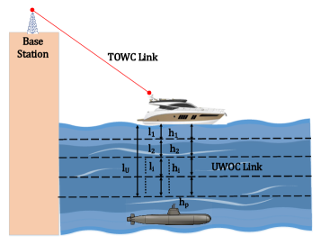
Figure 1: Mixed TWOC-UWOC system with multi-layer UWOC channel.

We consider a mixed terrestrial and underwater optical communication system integrated through a fixed-gain AF relaying protocol, as shown in Fig 1. Assume that a source on the land intends to communicate a signal $s$ with an underwater submarine. We use the non-coherent intensity modulation/direct detection (IM/DD) scheme, where the photodetector detects changes in the light intensity without employing a local oscillator. It is known that the heterodyne detection (HD) requires complex processing of mixing the received signal with a coherent signal produced by the local oscillator [34]. In the following two subsections, we describe channel and system models for terrestrial and underwater OWC systems.

II-A Terrestrial OWC

In the first hop, we assume that the transmitted signal undergoes three types of fading: atmospheric turbulence-induced, pointing errors, and random fog. Thus, the received signal $y_{T}$ at the relay is given by

$$y=h_{T}s+w_{T}$$ (1)

where $h_{T}$ is the channel coefficient (including fog-induced path gain, atmospheric turbulence, and pointing errors) for the terrestrial link and $w_{T}$ is the additive white gaussian noise (AWGN) with variance $\sigma_{w_{T}}^{2}$ Assuming generalized Malága distribution for atmospheric turbulence, fog-induced random path loss, and zero bore-sight pointing errors, then the PDF of the SNR $\gamma_{T}$for the terrestrial link is given by [35]

$$f_{\gamma_{T}}(x)=\frac{z^{k}\rho_{T}^{2}A^{\rm{mg}}}{4\gamma}\sum_{m_{1}=1}^{\beta^{M}}b^{M}_{m_{1}}$$

$$G_{1+k,3+k}^{3+k,0}\left(\begin{array}[]{c}\rho_{T}^{2}+1,\{z+1\}_{1}^{k}\\ \rho_{T}^{2},\alpha^{M},m_{1},\{z\}_{1}^{k}\end{array}\left|\frac{\alpha^{M}\beta^{M}\sqrt{\gamma}}{(g^{M}\beta^{M}+\Omega^{M})A_{T}\sqrt{\bar{\gamma}_{T}}}\right.\right)$$ (4)

where $\bar{\gamma}_{T}$ is the average SNR, $\{\alpha^{{\scriptscriptstyle M}},\beta^{{\scriptscriptstyle M}},A^{m\rm g},b_{m_{1}}^{M},g^{M},\Omega^{M}\}$ are Malága parameters [36], $\{\rho_{T},A_{T}\}$ are pointing error parameters [37], and $\{z,k\}$ specifies the effect of fog on the signal transmission [38].

II-B Underwater OWC

In the second hop, we employ a fixed-gain AF relay with gain parameter $G_{R}$ to forward the received to the destination over underwater channel. The gain selection $G_{R}$ can be entirely blind for a duration or using a semi-blind approach where it can be obtained using statistics of received signal power of the first hop (i.e., TOWC link). We consider the UWOC system by splitting the entire transmission channel in $N$ distinct layers in succession, resulting in $N$ vertical links, as depicted in Fig 1. Thus, the received electrical signal $y_{U}$ at the destination can be expressed as:

$$y_{U}=h_{l}h_{p}\left[\prod_{i=1}^{N}h_{i}\right]G_{R}y_{T}+w_{U}$$ (5)

where $h_{l}=e^{-\alpha l}$ is the path gain with link distance $l$ (in m) and extinction attenuation coefficient $\alpha$, $h_{p}$ models pointing errors, $h_{c}=\prod_{i=1}^{N}h_{i}$ is the cascaded channel with $h_{i}$ as the $i$-th layer of vertical link, and $w_{U}$ is the AWGN with variance $\sigma_{w_{U}}^{2}$.

The PDF of zero-boresight pointing errors fading $h_{p}$ is given as [37]:

$$f_{h_{p}}(x)=\frac{\rho^{2}}{A_{0}^{\rho^{2}}}h_{p}^{\rho^{2}-1},0\leq h_{p}\leq A_{0}$$ (6)

where $A_{0}=\mbox{erf}(\upsilon)^{2}$ with $\upsilon=\sqrt{\pi/2}\ r/\omega_{z}$, $r$ is the aperture radius and $\omega_{z}$ is the beam width, and $\rho={\frac{\omega_{{z}_{\rm eq}}}{2\sigma_{s}}}$ with $\omega_{{z}_{\rm eq}}$ as the equivalent beam width at the receiver and $\sigma^{2}_{s}$ as the variance of pointing errors displacement characterized by the horizontal sway and elevation [37].

Fading coefficients $h_{i}$, $i=1,2,\cdots,N$ associated with different layers are modeled using various statistical distributions such as generalized Gamma, EGG, GG, and EW among others for different underwater conditions [9, 11].

The PDF of the channel coefficient for the generalized Gamma is given as

$$f_{h_{i}}(x)=\frac{p_{i}}{{a_{i}}^{d_{i}}\Gamma\Big{(}\frac{d_{i}}{p_{i}}\Big{)}}{x}^{d_{i}-1}\exp\bigg{(}-\Big{(}\frac{x}{a_{i}}\Big{)}^{p_{i}}\bigg{)}$$ (7)

where $a_{i}$, $d_{i}$, and $p_{i}$ are distribution parameters for the $i$-th layer to model different oceanic turbulence scenarios, as given in [9] (see Table-I, Table-II, and Table-III). As such, $p_{i}=1$ in (7) denotes a Gamma distribution representing a thermally uniform UWOC channel.

Recently, [11] proposed EGG distribution (i.e., the combined exponential and generalized Gamma) for the oceanic turbulence with the PDF:

$$f_{h_{i}}(x)=\frac{\omega_{i}}{\lambda_{i}}\exp(-\frac{x}{\lambda_{i}})+$$

$$(1-\omega_{i})\frac{p_{i}}{{a_{i}}^{d_{i}}\Gamma\Big{(}\frac{d_{i}}{p_{i}}\Big{)}}{x}^{d_{i}-1}\exp\bigg{(}-\Big{(}\frac{x}{a_{i}}\Big{)}^{p_{i}}\bigg{)}$$ (8)

where $\omega_{i}$ is the mixture coefficient of the distributions (i.e, $0<\omega_{i}>1$), $\lambda_{i}$ is the exponential distribution parameter. Note that experimental data is available for $a_{i},p_{i}$, and $d_{i}/p_{i}$.

Further, the PDF of the channel coefficient using the three-parameter EW distribution to model the oceanic turbulence is given by:

$$f_{h_{i}}(x)=\frac{\alpha_{i}^{E}\beta_{i}^{E}}{\eta_{i}^{E}}\left(\frac{x}{\eta_{i}^{E}}\right)^{({\beta_{i}^{E}}-1)}\exp\left[-\left(\frac{x}{\eta_{i}^{E}}\right)\right]^{\beta_{i}^{E}}$$

$$\left[1-\exp\left[-\left(\frac{x}{\eta_{i}^{E}}\right)^{\beta_{i}^{E}}\right]\right]^{({\alpha_{i}^{E}}-1)}$$ (9)

where $\beta_{i}^{E}>0$ denotes the shape parameter of the scintillation index (SI), $\eta_{i}^{E}>0$ is a scale parameter, and $\alpha_{i}^{E}>0$ is an extra shape parameter dependent on the receiver aperture size [39].

Experimental studies also found the Gamma-Gamma PDF [40] a good fit for oceanic turbulent channel [9]:

$$f_{h_{i}}(x)=\frac{2(\alpha_{i}^{G}\beta_{i}^{G})^{(\alpha_{i}^{G}+\beta_{i}^{G})/2}}{\Gamma({\alpha_{i}^{G}})\Gamma({\beta_{i}^{G}})}x^{\frac{\alpha_{i}^{G}+\beta_{i}^{G}}{2}-1}$$

$$K_{\alpha_{i}^{G}-\beta_{i}^{G}}(2(\alpha_{i}^{G}\beta_{i}^{G}x)^{1/2})$$ (10)

In what follows, we unify the performance of multi-layer UWOC system over different oceanic turbulence models.

III Multi-Layer UWOC

In this section, we develop statistical analysis for the multi-layer underwater turbulence channel unifying generalized Gamma, EGG, GG, and EW oceanic turbulence models. We also analyze the UWOC performance by deriving outage probability, average BER, and ergodic capacity demonstrating the impact of multi-layer modeling for the vertical channel.

III-A Statistical Results

We use the inverse Mellin transform to find the PDF of $h_{c}=\prod_{i=1}^{N}h_{i}$ for a given oceanic turbulence. If $\mathbb{E}[X^{n}]$ denotes the $n$-th moment, where $\mathbb{E}[\cdot]$ denotes the expectation operator, then the inverse Mellin transform results the PDF of a random variable $X$ as

$$f_{X}(x)=\frac{1}{2\pi ix}\int_{\zeta-i\infty}^{\zeta+i\infty}x^{-n}\mathbb{E}[X^{n}]dn$$ (11)

where $\zeta-i\infty$ to $\zeta+i\infty$ denotes the line integral. It should be mentioned that Mellin transform has been used to analyze the product of $N$ random variable for different applications [41, 35, 42, 43]. Similar to [9], we assume that turbulence channels are independent for each layer to get the $n$-th order moment for $h_{c}$ as

$$\mathbb{E}[h_{c}^{n}]=\prod_{i=1}^{N}\int_{0}^{\infty}h_{i}^{n}f_{h_{i}}(h_{i})dh_{i}$$ (12)

In the following theorem, we use (12) in (11) to derive the PDF for various oceanic turbulence.

Theorem 1

An unified expression for the PDF of multi-layer UWOC channel distributing according to GG, EGG, $\Gamma\Gamma$, and EW is given by

$$f_{h_{c}}(h_{c})= \prod_{i=1}^{N}\mathcal{A}_{i}\sum_{j=0}^{\mathcal{P}}\mathcal{B}_{i,j}$$

$$\frac{1}{h_{c}}H_{0,q}^{m,0}\left[\begin{matrix}-\\ \{\mathcal{D}_{i_{1},j}\}_{i_{1}=1}^{N}\end{matrix}\bigg{|}\prod_{i_{2}=1}^{N}\mathcal{E}_{i_{2},j}h_{c}\right]$$ (13)

where $\mathcal{A}_{i}$, $\mathcal{P}$, $\mathcal{D}_{i_{1},j}$, $\mathcal{E}_{i_{2},j}$, $m$, and $q$ are given in Table II.

TABLE II: Unified Parameters

Oceanic Models	Unified Parameter Description
EGG	$\mathcal{P}=1,\mathcal{A}_{i}=1,\mathcal{B}_{i,0}=\omega_{i}$, $\mathcal{B}_{i,1}=\frac{(1-\omega_{i})}{\Gamma\left(\frac{d_{i}}{p_{i}}\right)}$, $m=N$, $q=N$, $\mathcal{D}_{i_{1},0}=(1,1)$, $\mathcal{D}_{i_{1},1}=\left(\frac{d_{i_{1}}}{p_{i_{1}}},\frac{1}{p_{i_{1}}}\right)$, $\mathcal{E}_{i_{2},0}=\frac{1}{\lambda_{i_{2}}}$, $\mathcal{E}_{i_{2},1}=\frac{1}{a_{i_{2}}}$
GG	$\mathcal{P}=0,\mathcal{A}_{i}=\frac{1}{\Gamma\left(\frac{d_{i}}{p_{i}}\right)},\mathcal{B}_{i,j}=1$, $m=N$, $q=N$, $\mathcal{D}_{i_{1},j}=\left(\frac{d_{i_{1}}}{p_{i_{1}}},\frac{1}{p_{i_{1}}}\right)$, $\mathcal{E}_{i_{2},j}=\frac{1}{a_{i_{2}}}$
EW	$\mathcal{P}=\infty,\mathcal{A}_{i}=\Gamma(\alpha^{E}_{i}+1),\mathcal{B}_{i,j}=\frac{(-1)^{j}}{(j+1)!\Gamma(\alpha^{E}_{i}-j)}$, $m=N$, $q=N$, $\mathcal{D}_{i_{1},j}=\left(1,\frac{1}{\beta^{E}_{i_{1}}}\right)$, $\mathcal{E}_{i_{2},j}=\frac{(j+1)^{\frac{1}{\beta^{E}_{i_{2}}}}}{\eta^{E}_{i_{2}}}$
$\Gamma\Gamma$	$\mathcal{P}=0,\mathcal{A}_{i}=\frac{1}{\Gamma(\alpha^{G}_{i})\Gamma(\beta^{G}_{i})},\mathcal{B}_{i,j}=1$, $m=2N$, $q=2N$, $\mathcal{D}_{i_{1},j}=\{(\alpha^{G}_{i_{1}},1),(\beta^{G}_{i_{1}},1)\}$, $\mathcal{E}_{i_{2},j}=\alpha^{G}_{i_{2}}\beta^{G}_{i_{2}}$

Proof:

See Appendix A.

∎

The derived PDF in Theorem 1 is represented using a single variate Fox-H function, which can be computed efficiently through computational software.

Next, we use the statistical result of Theorem 1 to analyze the multi-layer UWOC performance. Assuming IM/DD technique and on-off keying (OOK) modulation with $x\in\{0,\sqrt{2}P_{t}\}$ and $P_{t}$ as average transmitted optical, the instantaneous received electrical SNR is given by [37]

$$\gamma_{U}=\frac{P^{2}_{t}h^{2}_{l}h^{2}}{\sigma_{w}^{2}}=\bar{\gamma}_{U}h^{2}$$ (14)

where $h=h_{c}h_{p}$ is the combined channel and $\bar{\gamma}_{U}=\frac{P^{2}_{t}h^{2}_{l_{U}}}{\sigma_{wT}^{2}}$ is the average electrical SNR. Note that $P_{t}^{2}$ in (14) is attributed to the detection type IM/DD and becomes $\gamma_{U}=\frac{P_{t}h_{l_{U}}h}{\sigma_{wT}^{2}}$ for the HD technique [34, 35].

In the following Lemma, we provide PDF and CDF of the SNR for the UWOC vertical links under the combined effect of the oceanic turbulence and pointing errors:

Lemma 1

Unified expressions for PDF and CDF of the SNR for multi-layer UWOC system with pointing errors are given as:

$$f_{\gamma_{U}}(\gamma)=\prod_{i=1}^{N}\frac{\rho_{U}^{2}\mathcal{A}_{i}}{2}\sum_{j=0}^{\mathcal{P}}\mathcal{B}_{i,j}$$

$$\frac{1}{\gamma}H_{1,q+1}^{m+1,0}\left[\begin{matrix}(1+\rho_{U}^{2})\\ \{\mathcal{D}_{i_{1},j}\}_{i_{1}=1}^{N},(\rho_{U}^{2},1)\end{matrix}\bigg{|}\prod_{i_{2}=1}^{N}\frac{\mathcal{E}_{i_{2},j}}{A_{U}}\sqrt{\frac{\gamma}{\bar{\gamma}_{U}}}\right]$$ (15)

$$F_{\gamma_{U}}(\gamma)=\prod_{i=1}^{N}\frac{\rho_{U}^{2}\mathcal{A}_{i}}{2}\sum_{j=0}^{\mathcal{P}}\mathcal{B}_{i,j}$$

$$H_{2,q+2}^{m+1,1}\left[\begin{matrix}(1,1),(1+\rho_{U}^{2})\\ \{\mathcal{D}_{i_{1},j}\}_{i_{1}=1}^{N},(\rho_{U}^{2},1),(0,1)\end{matrix}\bigg{|}\prod_{i_{2}=1}^{N}\frac{\mathcal{E}_{i_{2},j}}{A_{U}}\sqrt{\frac{\gamma}{\bar{\gamma}_{U}}}\right]$$ (16)

Proof:

See Appendix B. ∎

III-B Outage Probability

Outage probability is a performance metric which demonstrate the effect of fading channel on the communication systems. It is defined as the probability that the SNR falls below a certain threshold $\gamma_{\rm th}$ and is given as

$$P_{\text{out}}=P(\gamma<\gamma_{\text{th}})=F_{\gamma}(\gamma_{\text{th}})$$ (17)

where $\gamma_{\rm th}$ is the SNR threshold. Substituting (16) in (17) yields an exact expression for the outage probability. The asymptotic expression for the outage probability in the high SNR regime $\bar{\gamma}_{U}\to\infty$ can be derived by applying [44, eq. $1.8.4$]:

$$P_{\rm{out}}^{\infty}=\prod_{i=1}^{N}\frac{\rho_{U}^{2}\mathcal{A}_{i}}{2}\sum_{j=0}^{\mathcal{P}}\mathcal{B}_{i,j}\sum_{k=1}^{m+1}$$

$$\frac{\left(\frac{\mathcal{E}_{i_{2},j}}{A_{U}}\sqrt{\frac{\gamma_{\rm th}}{\bar{\gamma}_{U}}}\right)^{\frac{b_{k}}{\beta_{k}}}\prod_{j=1,j\neq k}^{m+1}\Gamma\left(b_{j}-b_{k}\frac{\beta_{j}}{\beta_{k}}\right)\Gamma\left(\frac{b_{k}}{\beta_{k}}\right)}{\beta_{k}\Gamma\left(1+\rho_{U}^{2}-\frac{b_{k}}{\beta_{k}}\right)\Gamma\left(1+\frac{b_{k}}{\beta_{k}}\right)}$$ (18)

where $b_{j}=b_{k}=\{\rho_{U}^{2},[\mathcal{D}_{i_{1},j}]_{1}\}$ and $\beta_{j}=\beta_{k}=\{1,[\mathcal{D}_{i_{1},j}]_{2}\}$.

The dominant SNR terms of (18) provides the diversity of proposed system as ${DO}_{{\rm out}}=\min\{\sum_{i=1}^{N}\frac{b_{k}}{2\beta_{k}}\}$. Using Table II, the diversity order for the EGG, GG, EW and $\Gamma\Gamma$ oceanic turbulence can be derived as: ${DO}_{{\rm EGG}}=\min\{\frac{N}{2},\sum_{i=1}^{N}\frac{d_{i}}{2},\frac{\rho_{U}^{2}}{2}\}$, ${DO}_{{\rm GG}}=\min\{\sum_{i=1}^{N}\frac{d_{i}}{2},\frac{\rho_{U}^{2}}{2}\}$, ${DO}_{{\rm EW}}=\min\{\sum_{i=1}^{N}\frac{\beta_{i}^{E}}{2},\frac{\rho_{U}^{2}}{2}\}$, and ${DO}_{\Gamma\Gamma}=\min\{\sum_{i=1}^{N}\frac{\alpha_{i}^{G}}{2},\sum_{i=1}^{N}\frac{\beta_{i}^{G}}{2},\frac{\rho_{U}^{2}}{2}\}$, respectively. The diversity order provides deployment strategies for oceanic turbulence models and the beam-width of optical transmissions. As such, beam-width can be adjusted sufficiently to mitigate the effect of pointing errors.

III-C Average BER

In this subsection, we derive the average BER for the proposed UWOC system. Considering IM/DD, the average BER can be obtained as [45]:

$$\overline{BER}=\frac{\delta}{2\Gamma(\phi)}\sum_{n=1}^{M^{\prime}}q_{n}^{\phi}\int_{0}^{\infty}\gamma^{\phi-1}{\exp(-q_{n}\gamma)}F_{\gamma}(\gamma)d\gamma$$ (19)

where the set $\{M^{\prime},\delta,\phi,q_{n}\}$ can specify a variety of modulation schemes.

Using (16) and substituting $\exp(-q_{n}\gamma)=G_{0,1}^{1,0}\left[\begin{matrix}-\\ 0\end{matrix}\bigg{|}q_{n}\gamma\right]$ in (19) and reduce the Meijer’s G-function into Fox-H function, we get

$$\overline{BER}_{U}=\frac{\delta\rho_{U}^{2}}{2\Gamma(\phi)}\sum_{n=1}^{M^{\prime}}q_{n}^{\phi}\prod_{i=1}^{N}\mathcal{A}_{i}\sum_{j=0}^{\mathcal{P}}\mathcal{B}_{i,j}$$

$$\int_{0}^{\infty}\gamma^{\phi-1}H_{0,1}^{1,0}\left[\begin{matrix}-\\ (0,1)\end{matrix}\bigg{|}q_{n}\gamma\right]H_{p+2,q+2}^{m+1,n+1}$$

$$\left[\begin{matrix}(1,1),(1+\rho_{U}^{2})\\ \{\mathcal{D}_{i_{1},j}\}_{i_{1}=1}^{N},(\rho_{U}^{2},1),(0,1)\end{matrix}\bigg{|}\prod_{i_{2}=1}^{N}\frac{\mathcal{E}_{i_{2},j}}{A_{U}}\sqrt{\frac{\gamma}{\bar{\gamma}_{U}}}\right]d\gamma$$

(20)

Finally, we apply the identity [44, eq. $2.8.4$] to get the closed-form expression for the average BER of the multi-layer UWOC channel:

$$\overline{BER}_{U}=\frac{\delta\rho_{U}^{2}}{2\Gamma(\phi)}\sum_{n=1}^{M^{\prime}}\prod_{i=1}^{N}\mathcal{A}_{i}\sum_{j=0}^{\mathcal{P}}\mathcal{B}_{i,j}H_{p+3,q+2}^{m+1,n+1}$$

$$\left[\begin{matrix}(1,1),(1-\phi,\frac{1}{2}),(1+\rho_{U}^{2})\\ \{\mathcal{D}_{i_{1},j}\}_{i_{1}=1}^{N},(\rho_{U}^{2},1),(0,1)\end{matrix}\bigg{|}\prod_{i_{2}=1}^{N}\frac{\mathcal{E}_{i_{2},j}}{A_{U}\sqrt{q_{n}\bar{\gamma}_{U}}}\right]$$

(21)

Similar to the outage probability, the asymptotic expression for average BER at high SNR $\bar{\gamma}_{U}\to\infty$ can be derived as

$$\overline{BER}_{U}^{\infty}=\frac{\delta\rho_{U}^{2}}{2\Gamma(\phi)}\sum_{n=1}^{M^{\prime}}\prod_{i=1}^{N}\mathcal{A}_{i}\sum_{j=0}^{\mathcal{P}}\mathcal{B}_{i,j}\sum_{k=1}^{m+1}$$

$$\frac{\left(\frac{\mathcal{E}_{i_{2},j}}{A_{U}\sqrt{q_{n}\bar{\gamma}_{U}}}\right)^{\frac{b_{k}}{\beta_{k}}}\prod_{j=1,j\neq k}^{m+1}\Gamma\left(b_{j}-b_{k}\frac{\beta_{j}}{\beta_{k}}\right)\Gamma\left(\frac{b_{k}}{\beta_{k}}\right)\Gamma\left(\phi+\frac{b_{k}}{2\beta_{k}}\right)}{\beta_{k}\Gamma\left(1+\rho_{U}^{2}-\frac{b_{k}}{\beta_{k}}\right)\Gamma\left(1+\frac{b_{k}}{\beta_{k}}\right)}$$ (22)

where $b_{j}=b_{k}=[\mathcal{D}_{i_{1},j}]_{1}$ and $\beta_{j}=\beta_{k}=[\mathcal{D}_{i_{1},j}]_{2}$.

Thus, the dominant SNR terms of (22) provides the diversity of proposed system as $\min\{\sum_{i=1}^{N}\frac{b_{k}}{2\beta_{k}}\}$, which is exactly same as obtained using the outage probability.

III-D Ergodic Capacity

The ergodic capacity for the underwater link $\overline{EC}_{U}$ is an important performance metric for the design of communication systems and it can be defined as [46]:

$$\overline{EC}_{U} =\int\limits_{0}^{\infty}\log_{2}(1+\kappa\gamma)f_{\gamma_{U}}(\gamma)d\gamma$$ (23)

where $\kappa=\frac{e}{2\pi}$ for IM/DD and $\kappa=1$ for HD (heterodyne detection).

Using (15) and substituting $\log_{2}(1+\kappa\gamma)=1.44G_{2,2}^{1,2}\left[\begin{matrix}1,1\\ 1,0\end{matrix}\bigg{|}\kappa\gamma\right]$ in (23) and reduce the Meijer’s G-function into Fox-H function, we get

$$\overline{EC}_{U}=0.72\rho_{U}^{2}\prod_{i=1}^{N}\mathcal{A}_{i}\sum_{j=0}^{\mathcal{P}}\mathcal{B}_{i,j}$$

$$\int_{0}^{\infty}\gamma^{-1}H_{2,2}^{1,2}\left[\begin{matrix}(1,1),(1,1)\\ (1,1),(0,1)\end{matrix}\bigg{|}\kappa\gamma\right]$$

$$H_{p+1,q+1}^{m+1,n}\left[\begin{matrix}(1+\rho_{U}^{2})\\ \{\mathcal{D}_{i_{1},j}\}_{i_{1}=1}^{N},(\rho_{U}^{2},1)\end{matrix}\bigg{|}\prod_{i_{2}=1}^{N}\frac{\mathcal{E}_{i_{2},j}}{A_{U}}\sqrt{\frac{\gamma}{\bar{\gamma}_{U}}}\right]d\gamma$$

(24)

Finally, we applying the identity [44, eq. $2.8.4$] to get the closed-form expression for the ergodic capacity over the cascaded channel

$$\overline{EC}=0.72\rho_{U}^{2}\prod_{i=1}^{N}\mathcal{A}_{i}\sum_{j=0}^{\mathcal{P}}\mathcal{B}_{i,j}H_{p+3,q+3}^{m+3,n+1}$$

$$\left[\begin{matrix}(0,\frac{1}{2}),(1,\frac{1}{2}),(1+\rho_{U}^{2},1)\\ \{\mathcal{D}_{i_{1},j}\}_{i_{1}=1}^{N},(\rho_{U}^{2},1)(0,\frac{1}{2}),(0,\frac{1}{2})\end{matrix}\bigg{|}\prod_{i_{2}=1}^{N}\frac{(\kappa\bar{\gamma}_{U})^{-\frac{1}{2}}}{A_{U}}\right]$$

(25)

In what follows, we employ a terrestrial optical link to communicate with the underwater transmission.

IV Performance of Mixed TOWC-UWOC System

In this section, we analyze the performance of a mixed TOWC-UWOC system when the fixed-gain AF relaying is applied. We can use (5) to express the end-to-end SNR of the dual-hop system consisting of TOWC and UWOC links [47]:

$${\gamma}=\frac{\gamma_{T}\gamma_{U}}{\gamma_{U}+C}$$ (26)

where $C$ a constant for the fixed-gain AF relaying protocol. Standard transformation of random variables in (26) leads to th the PDF of SNR for the fixed-gain AF relayed system as

$$f_{\gamma}(\gamma)=\int_{0}^{\infty}{f_{\gamma_{T}}\left(\frac{\gamma(x+C)}{x}\right)}{f_{\gamma_{U}}(x)}\frac{x+C}{{x}}{dx}$$ (27)

where $f_{\gamma_{T}}(\gamma)$ and $f_{\gamma_{U}}(\gamma)$ are the PDF of SNR for TOWC link and UWOC link, respectively.

We use (4) and (15) in (27) to develop the PDF of the SNR for the mixed link:

Lemma 2

The PDF and CDF of the end-to-end SNR for the fixed-gain AF relay-assisted mixed TWOC-UWOC system are given as

$$f_{\gamma}(\gamma)=\frac{z^{k}\rho_{T}^{2}A^{\rm{mg}}}{4\gamma}\sum_{m_{1}=1}^{\beta^{M}}b^{M}_{m_{1}}\prod_{i=1}^{N}\frac{\rho_{U}^{2}\mathcal{A}_{i}}{2}\sum_{j=0}^{\mathcal{P}}\mathcal{B}_{i,j}$$

$$H_{1,0:3+k,k+2;1,m+2}^{0,1:0,3+k;m+2,0}\Bigg{[}\begin{array}[]{c}\frac{(g^{M}\beta^{M}+\Omega^{M})A_{T}\sqrt{\bar{\gamma}_{T}}}{\alpha^{M}\beta^{M}\sqrt{\gamma}}\\ \frac{\mathcal{E}_{i_{2},j}}{A_{U}}\sqrt{\frac{1}{\bar{\gamma}_{U}}}\end{array}\bigg{|}\begin{array}[]{c}U_{1}\\ V_{1}\end{array}\Bigg{]}$$ (32)

where $U_{1}=\{(1:\frac{1}{2},\frac{1}{2}):(1-\rho_{T}^{2},1);(1-\alpha^{M},1);(1-m_{1},1);\{(1-z,1)\}^{k}_{1};(1+\rho_{U}^{2},1)\}$ and $V_{1}=\{-:(-\rho_{T}^{2},1);(-z,1);(1,\frac{1}{2});\{\mathcal{D}_{i_{1},j}\}_{i_{1}=1}^{N};(\rho_{U}^{2},1);(0,\frac{1}{2})\}$.

$$F_{\gamma}(\gamma)=\frac{z^{k}\rho_{T}^{2}A^{\rm{mg}}}{4}\sum_{m_{1}=1}^{\beta^{M}}b^{M}_{m_{1}}\prod_{i=1}^{N}\frac{\rho_{U}^{2}\mathcal{A}_{i}}{2}\sum_{j=0}^{\mathcal{P}}\mathcal{B}_{i,j}$$

$$H_{1,0:4+k,3+k;1,2+m}^{0,1:0,4+k;2+m,0}\Bigg{[}\begin{array}[]{c}\frac{(g^{M}\beta^{M}+\Omega^{M})A_{T}\sqrt{\bar{\gamma}_{T}}}{\alpha^{M}\beta^{M}\sqrt{\gamma}}\\ \frac{\mathcal{E}_{i_{2},j}}{A_{U}}\sqrt{\frac{1}{\bar{\gamma}_{U}}}\end{array}\big{|}\begin{array}[]{c}U_{2}\\ V_{2}\end{array}\Bigg{]}$$ (37)

where $U_{2}=\{(1:\frac{1}{2},\frac{1}{2}):(1-\rho_{T}^{2},1);(1-\alpha^{M},1);(1-m_{1},1);\{(1-z,1)\}^{k}_{1};(1,\frac{1}{2});(1+\rho_{U}^{2},1)\}$ and $V_{2}=\{-:(-\rho_{T}^{2},1);(-z,1);(1,\frac{1}{2});(0,\frac{1}{2});\{\mathcal{D}_{i_{1},j}\}_{i_{1}=1}^{N};(\rho_{U}^{2},1);(0,\frac{1}{2})\}$

TABLE III: Simulation Parameters

Transmitted optical power	$P_{t}$	$-10$ to $60$ dBm
AWGN variance	$\sigma_{w}^{2}$	$10^{-14}~{}\rm{A^{2}/GHz}$
Total link distance	$l$	$l=(l_{T}+l_{U})=(400+50)$ m
Extinction coefficient	$\alpha$	$0.056$
Shape parameter of foggy channel	$k$	{13.12, 12.06}
Scale parameter of foggy channel	$\beta^{f}$	{2, 5}
Pointing errors parameters	$A$, $\rho^{2}$	$0.0032$, $\{1,6\}$
Malága distribution parameters [35]	$\alpha^{M}$	$\{4.5916,2.3378,1.4321\}$
	$\beta^{M}$	$\{7.0941,4.5323,3.4948\}$
	$\{a_{i}\}_{i=1}^{5}$	$\{0.6302,1.0750,1.0173,0.7598,1.0990\}$
GG distribution parameters [9]	$\{d_{i}\}_{i=1}^{5}$	$\{1.1780,3.2048,1.6668,2.3270,4.5550\}$
	$\{p_{i}\}_{i=1}^{5}$	$\{0.8444,2.9222,1.0380,1.4353,4.6208\}$
EGG distribution parameters [11]	$\{\omega_{i}\}_{i=1}^{2}$	$\{0.1770,0.4589\}$
	$\{\lambda_{i}\}_{i=1}^{2}$	$\{0.4687,0.3449\}$
	$\{\omega_{i}\}_{i=1}^{5}$	$\{0.2130,0.2108,0.1807,0.1665,0.4589\}$
	$\{\lambda_{i}\}_{i=1}^{5}$	$\{0.3291,0.2694,0.1641,0.1207,0.3449\}$
EGG distribution parameters (For Fig. 5(a) and Fig. 5(b)) [11]	$\{\frac{d_{i}}{p_{i}}\}_{i=1}^{5}$	$\{1.4299,0.6020,0.2334,0.1559,1.0421\}$
	$\{a_{i}\}_{i=1}^{5}$	$\{1.1817,1.2795,1.4201,1.5216,1.5768\}$
	$\{p_{i}\}_{i=1}^{5}$	$\{17.1984,21.1611,22.5924,22.8754,35.9424\}$
EW distribution parameters [9]	$\alpha^{E}$, $\beta^{E}$, $\eta^{E}$	$2.50$, $0.70$, $0.50$
$\Gamma\Gamma$ distribution parameters [9]	$\alpha^{G}$, $\beta^{G}$	$5$, $1.18$
Modulation parameters	$M^{\prime}$, $\delta$, $\phi$, $q_{n}$	$1$, $1$, $\frac{1}{2}$, $\frac{1}{2}$

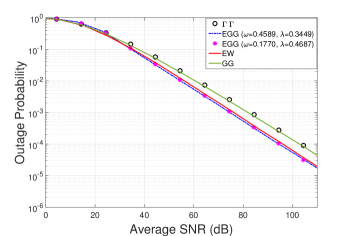
(a) Single-layer ($N=1$) with $\rho_{U}^{2}=1$.

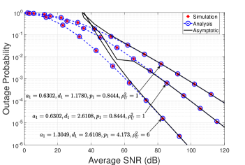
(b) Multi-layer ($N=5$) with GG oceaninc turbulence.

Figure 2: Outage probability performance.

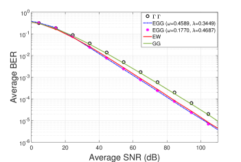
(a) Single-layer ($N=1$) for various oceaninc turbulence.

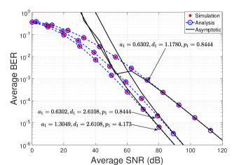
(b) Multi-layer ($N=5$) with GG oceaninc turbulence and $\rho_{U}^{2}=6$.

Figure 3: Average BER performance.

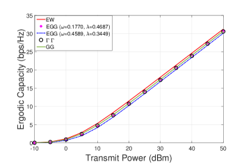
(a) Single-layer ($N=1$) for various oceaninc turbulence.

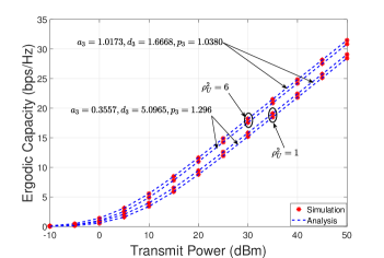
(b) Multi-layer ($N=5$) with GG oceaninc turbulence.

Figure 4: Ergodic capacity performance.

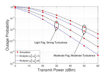
(a) Outage probability.

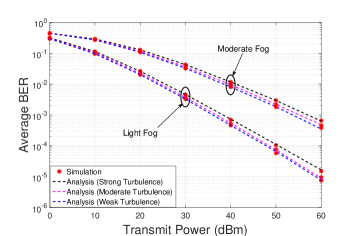
(b) Average BER with $\rho_{T}^{2}=6$, and $\rho_{U}^{2}=6$.

Figure 5: Outage and error performance of mixed TWOC and multi-layer UWOC with EGG oceanic turbulence.

Proof:

See Appendix C. ∎

There are standard routines to compute bivariate Fox-H function in MATLAB. Further, we can use the CDF in (2) to derive the outage probability of the mixed TWOC-UWOC system as $P_{\text{out}}=F_{\gamma}(\gamma_{\text{th}})$ given a threshold SNR $\gamma_{\rm th}$.

Finally, we use (2) in (19) to find the average BER of the mixed TWOC-UWOC system as

$$\overline{BER}=\frac{\delta}{2\Gamma(\phi)}\sum_{n=1}^{M^{\prime}}q_{n}^{\phi}\frac{z^{k}\rho_{T}^{2}A^{\rm{mg}}}{4}\sum_{m_{1}=1}^{\beta^{M}}b^{M}_{m_{1}}\bigg{(}\frac{1}{2\pi\jmath}\bigg{)}^{2}$$

$$\int_{\mathcal{L}_{1}}\int_{\mathcal{L}_{2}}\prod_{i=1}^{N}\frac{\rho_{U}^{2}\mathcal{A}_{i}}{2}\sum_{j=0}^{\mathcal{P}}\mathcal{B}_{i,j}\bigg{(}\frac{(g^{M}\beta^{M}+\Omega^{M})A_{T}\sqrt{\bar{\gamma}_{T}}}{\alpha^{M}\beta^{M}\sqrt{\gamma}}\bigg{)}^{-n_{1}}$$

$$\frac{\Gamma(\rho_{T}^{2}-n_{1})\Gamma(\alpha^{M}-n_{1})\Gamma(m_{1}-n_{1})[\Gamma(z-n_{1})]^{k}_{1}}{\Gamma(\rho_{T}^{2}+1-n_{1})[\Gamma(z+1-n_{1})]^{k}_{1}\Gamma(-\frac{n_{1}}{2})}$$

$$\bigg{(}\frac{\mathcal{E}_{i_{2},j}}{A_{U}}\sqrt{\frac{1}{\bar{\gamma}_{U}}}\bigg{)}^{-n_{2}}\frac{\prod_{j=1}^{m}[\Gamma(\mathcal{D}_{i,j})]^{N}_{i=1}\Gamma(\rho_{U}^{2}+n_{2})\Gamma(\frac{n_{2}}{2})}{\Gamma(\rho_{U}^{2}+1+n_{2})}$$

$$\Gamma\left(-\frac{n_{1}}{2}-\frac{n_{2}}{2}\right)\bigg{(}\int_{0}^{\infty}\gamma^{\phi-\frac{n_{1}}{2}-1}\exp(-q_{n}\gamma)\mathop{}\!d\gamma\bigg{)}\mathop{}\!dn_{1}\mathop{}\!dn_{2}$$ (38)

Solving the inner integral as $\int_{0}^{\infty}\gamma^{\phi-\frac{n_{1}}{2}-1}\exp(-q_{n}\gamma)\mathop{}\!d\gamma=\Gamma\left(\phi-\frac{n_{1}}{2}\right)q^{-\phi+\frac{n_{1}}{2}}_{n}$ and applying [48], we get average BER of the mixed TWOC-UWOC system involving the bivariate Fox-H function:

$$\overline{BER}=\frac{\delta}{2\Gamma(\phi)}\sum_{n=1}^{M^{\prime}}\frac{z^{k}\rho_{T}^{2}A^{\rm{mg}}}{4}\sum_{m_{1}=1}^{\beta^{M}}b^{M}_{m_{1}}\prod_{i=1}^{N}\frac{\rho_{U}^{2}\mathcal{A}_{i}}{2}\sum_{j=0}^{\mathcal{P}}\mathcal{B}_{i,j}$$

$$H_{1,0:5+k,3+k;1,2+m}^{0,1:0,5+k;2+m,0}\Bigg{[}\begin{array}[]{c}\frac{(g^{M}\beta^{M}+\Omega^{M})A_{T}\sqrt{\bar{\gamma}_{T}}}{\alpha^{M}\beta^{M}\sqrt{q_{n}}}\\ \frac{\mathcal{E}_{i_{2},j}}{A_{U}}\sqrt{\frac{1}{\bar{\gamma}_{U}}}\end{array}\big{|}\begin{array}[]{c}U_{3}\\ V_{3}\end{array}\Bigg{]}$$ (43)

where $U_{3}=\{(1:\frac{1}{2},\frac{1}{2}):(1-\rho_{T}^{2},1);(1-\alpha^{M},1);(1-m_{1},1);\{(1-z,1)\}^{k}_{1};(1,\frac{1}{2});\left(1-\phi,\frac{1}{2}\right);(1+\rho_{U}^{2},1)\}$ and $V_{3}=\{-:(-\rho_{T}^{2},1);(-z,1);(1,\frac{1}{2});(0,\frac{1}{2});\{\mathcal{D}_{i_{1},j}\}_{i_{1}=1}^{N};(\rho_{U}^{2},1);(0,\frac{1}{2})\}$ It should be mentioned that bivariate Fox-H function has been extensively analyzing the fixed-gain AF relaying over complicated fading models [27].

V Simulation and numerical analysis

In this section, we demonstrate the performance of multi-layer vertical UWOC system over-various oceanic turbulence conditions and the mixed TOWC-UOWC transmission. We also compare the performance of the multi-layer UWOC with the single-layer ($N=1$) approximation. We use Monte-Carlo (MC) simulation (averaged over $10^{7}$ channel realizations) to validate the derived analytical expressions. Further, the asymptotic expression of outage probability and average BER converges with analysis and simulation results in the high SNR regime. We use standard inbuilt MATLAB and Mathematica libraries to calculate Meijer’s G and Fox’s H-function, respectively. Since there is no measurement data to confirm the variation of distribution parameters with distance, we illustrate the performance by considering vertical underwater link length $l_{U}=50$ m with $N=5$ layers, and the thickness of each layer is assumed to be $10$ m. We use standard simulation parameters and measurement-based parametric data for EGG, GG, EW, and $\Gamma\Gamma$, as given in Table III.

First, we demonstrate the outage probability performance of the considered UWOC system in Fig. 2. It can be seen from Fig. 2(a) that the outage probability for a specific oceanic turbulence condition using different statistical models is similar for the single-layer ($N=1$) case validating the equivalence of different models using PDF plots, as demonstrated comprehensively in [9]. We used two different EGG turbulence since $\lambda$ and $\omega$ parameters is not available for the same experimental scenario. The figure shows that an acceptable operating outage probability of $10^{-3}$ can be achieved with an average SNR of $80$dB. To demonstrate the multi-layer performance, we consider the GG model (as depicted in Fig. 2(b) ), which excellently fits the experimental data for a wide range of oceanic turbulence, as observed in [9]. Comparing Fig. 2(a) and Fig. 2(b) with $\rho_{U}^{2}=1$ plots, it can be seen that the single-layer model underestimates the oceanic turbulence concerning the $N=5$ layers case justifying the use of multi-layer modeling for UWOC transmissions. Further, Fig. 2(b) shows that the outage performance of the system improves with an increase in the values of GG distribution parameters ($a$, $d$, and $p$) and a decrease in pointing errors (i.e., higher $\rho_{U}^{2}$). In the first plot of Fig. 2(b), we consider the pointing errors parameter ($\rho_{U}^{2}=1$) and the GG distribution parameters ($a$, $d$, and $p$) as given in Table III. The diversity order ${DO}_{\rm out}=\min\{\sum_{i=1}^{N}\frac{d_{i}}{2},\frac{\rho_{U}^{2}}{2}\}$ for the top and middle plots in Fig. 2(b) are given by $\min\{6.4658,0.5\}$ and $\min\{7.1822,0.5\}$, respectively. It can be clearly observed that the diversity order is dependent on the pointing error parameter ($\rho_{U}^{2}$) since the slope does not change with the oceanic channel parameter $d_{i}$. Further, in the third plot, the diversity order becomes $\min\{7.1822,3\}$, demonstrating a change of slope with $\rho_{U}^{2}$, thus confirming our diversity order analysis.

Next, we present the average BER performance of the single-layer system in Fig. 3(a) and multi-layer UWOC in Fig. 3(b). Similar to the outage probability, the average BER of the system provides similar observations with respect to the comparison of single-layer and multi-layer models and follows a similar trend with turbulent channel and pointing error parameters, as shown in Fig. 3(b). It is evident from the plots that the average BER of the system improves by almost ten times if we increase the channel parameter $d_{i}$ from $1.1780$ to $2.6108$ at average SNR of $80$ dB. The diversity order follows a similar analysis as that of the outage probability, which can be confirmed by observing the slope change among the plots.

In Fig. 4(a) and Fig. 4(b), we plot ergodic capacity performance for the single-layer ($N=1$) and multi-layer ($N=5$) UWOC systems, respectively. The ergodic capacity for different UWOC models is almost equal for the given oceanic conditions, as shown in Fig. 4(a). Further, the ergodic capacity is around $10$bits/sec/Hz at a nominal transmit power of $20$dBm. In Fig. 4(b), the effect of GG parameters is demonstrated for the multi-layer UWOC transmission. The figure shows that the ergodic capacity increases by almost $3{\rm{bits/sec/Hz}}$ if the pointing error parameter $\rho_{U}^{2}$ increases from $1$ to $6$ for the given turbulent parameters. It can also been seen that the ergodic capacity increases by almost $1{\rm{bits/sec/Hz}}$ if we change the oceanic turbulence parameters ($a_{3}=0.3557$, $d_{3}=5.0965$, and $p_{3}=1.296$) for the both $\rho_{U}^{2}=1$ and $\rho_{U}^{2}=6$.

Finally, we demonstrate the outage probability and average BER performance of the mixed TWOC and multi-layer ($N=5$) UWOC system in Fig. 5(a) and Fig. 5(b), respectively. We consider terrestrial link distance $l_{T}=400$ m, underwater link length $l_{U}=50$ m with $N=5$ layers each with EGG oceanic turbulence. In Fig. 5(a), we plot the outage probability considering light fog with weak turbulence and moderate fog with moderate turbulence for two different pointing errors parameters $\rho_{T}^{2}=\rho_{U}^{2}=\{1,6\}$. The effect of fog density, the intensity of atmospheric turbulence, and pointing errors are clearly visible. It can be seen from Fig. 5(a), that $20$ dBm more transmit power is required to achieve the same outage probability with moderate fog as compared with light fog. Further, the penalty for strong pointing errors is $10$dBm for the same foggy and atmospheric conditions. In Fig. 5(b), we demonstrate the effect of different (weak, moderate, and strong) atmospheric turbulence on the average BER performance for both light and moderate foggy conditions. The figure shows that the effect of atmospheric turbulence on the average BER performance is less as compared with performance degradation due to the fog.

VI Conclusions and Future Work

We presented unified performance analysis of the UWOC system considering the vertical underwater link as a multi-layer cascaded channel considering i.ni.d. GG, EGG, EW, and $\Gamma\Gamma$ oceanic turbulence channels. We analyzed the system performance by deriving analytical expressions of the PDF and CDF of the end-to-end SNR, and developed outage probability, average BER, and ergodic capacity under the combined effect of cascaded oceanic turbulence and pointing errors in terms of Meijer-G and Fox-H functions. We provided the asymptotic expressions using Gamma functions for the outage probability and average BER to determine the diversity order of the considered system. We also employed the fixed-gain AF relaying to integrate the terrestrial OWC transmission subjected to the combined effect of generalized Malága atmospheric turbulence, fog-induced random path gain, and pointing errors to communicate with the UWOC link. We analyzed the performance of the mixed link using outage probability and average BER involving bivariate Fox H-function. Simulation results showed a performance gap when the single-layer approximation was compared with the multi-layer model. The proposed analysis would be helpful for an efficient deployment for UWOC under various oceanic conditions. The existing measurement data and statistical model do not consider depth dependency for oceanic turbulence. It would be interesting to investigate the applicability of the proposed analysis using the channel measurement data considering ocean stratification for the UWOC system.

Appendix A: Proof of Theorem 1

First, we find the PDF of $h_{\rm GG}=\prod_{i=1}^{N}h_{i}$, where $h_{i}$, $i=1,2,\cdots,N$ denote i.ni.d GG random variables. Substituting (7) in (12) and applying the identity $\int_{0}^{\infty}t^{a}\exp(-bt^{c})dt=\frac{\Gamma\left(\frac{1+a}{c}\right)}{cb^{\frac{1+a}{c}}}$ [49, pp. $347$, eq. $3.381.10$], we get the $n$-th order moment of $h_{c}$ as:

$$\mathbb{E}[h_{\rm GG}^{n}]=\prod_{i=1}^{N}\frac{\Gamma\left(\frac{n+d_{i}}{p_{i}}\right)}{a_{i}^{-n}\Gamma\left(\frac{d_{i}}{p_{i}}\right)}$$ (44)

We use (44) in (11) and apply the definition of Fox H-function to get the PDF of $h_{c}$ for the generalized Gamma turbulent channel as

$$f_{h_{GG}}(x)=\prod_{i=1}^{N}\frac{1}{\Gamma\left(\frac{d_{i}}{p_{i}}\right)}$$

$$\frac{1}{x}H_{0,N}^{N,0}\left[\begin{matrix}-\\ \left\{\left(\frac{d_{i_{1}}}{p_{i_{1}}},\frac{1}{p_{i_{1}}}\right)\right\}_{i_{1}=1}^{N}\end{matrix}\bigg{|}\prod_{i_{2}=1}^{N}\left(\frac{x}{a_{i_{2}}}\right)\right]$$ (45)

Next, we find the PDF of $h_{\rm EGG}=\prod_{i=1}^{N}h_{i}$, where $h_{i}$, $i=1,2,\cdots,N$ denote i.ni.d EGG random variables. Substituting (8) in (12), we get the $n$-th order moment of $h_{\rm EGG}$ as:

$$\mathbb{E}[h_{\rm EGG}^{n}]=\prod_{i=1}^{N}\Bigg{(}\omega_{i}\lambda_{i}^{n}\Gamma(1+n)+\frac{(1-\omega_{i})\Gamma\left(\frac{n+d_{i}}{p_{i}}\right)}{a_{i}^{-n}\Gamma\left(\frac{d_{i}}{p_{i}}\right)}\Bigg{)}$$ (46)

Using (46) in (11) and applying the definition of Fox H-function to get the PDF of $h_{\rm EGG}$ for the EGG oceanic turbulent channel:

$$f_{h_{\rm EGG}}(x)=\prod_{i=1}^{N}\Bigg{(}\frac{\omega_{i}}{x}H_{0,N}^{N,0}\left[\begin{matrix}-\\ \{(1,1)\}_{i_{1}=1}^{N}\end{matrix}\bigg{|}\prod_{i_{2}=1}^{N}\frac{x}{\lambda_{i_{2}}}\right]+$$

$$\frac{(1-\omega_{i})}{\Gamma\left(\frac{d_{i}}{p_{i}}\right)x}H_{0,N}^{N,0}\left[\begin{matrix}-\\ \left\{\left(\frac{d_{i_{1}}}{p_{i_{1}}},\frac{1}{p_{i_{1}}}\right)\right\}_{i_{1}=1}^{N}\end{matrix}\bigg{|}\prod_{i_{2}=1}^{N}\left(\frac{x}{a_{i_{2}}}\right)\right]\Bigg{)}$$ (47)

To develop the PDF for the EW channel, we use the Newton’s generalized binomial theorem $(1+z)^{p}=\sum_{j=0}^{\infty}\frac{\Gamma(p+1)z^{j}}{j!\Gamma(p-j+1)}$ for the term $[1-(\exp(-x/\eta))^{\beta}]^{\alpha-1}$ in (9) to get

$$f_{h_{i}}(x)=\frac{\alpha^{E}_{i}\beta^{E}_{i}\Gamma(\alpha^{E}_{i})}{\eta^{E}_{i}}\sum_{j=0}^{\infty}\frac{(-1)^{j}}{j!\Gamma(\alpha^{E}_{i}-j)}\bigg{(}\frac{x}{\eta^{E}_{i}}\bigg{)}^{({\beta^{E}_{i}}-1)}$$

$$\exp\bigg{(}-(j+1)\big{(}\frac{x}{\eta^{E}_{i}}\big{)}^{\beta^{E}_{i}}\bigg{)}$$ (48)

Substituting (48) in (12) and applying the identity $\int_{0}^{\infty}t^{a}\exp(-bt^{c})dt=\frac{\Gamma\left(\frac{1+a}{c}\right)}{cb^{\frac{1+a}{c}}}$ [49, pp. $347$, eq. $3.381.10$], we get the $n$-th order moment of $h_{\rm EW}$ as:

$$\mathbb{E}(h_{\rm EW}^{n})=\prod_{i=1}^{N}\Gamma(\alpha_{i}+1)\sum_{j=0}^{\infty}\frac{(-1)^{j}}{j!\Gamma(\alpha_{i}-j)(j+1)}$$

$$\Gamma\left(1+\frac{n}{\beta_{i}}\right)\left(\frac{(j+1)^{\frac{1}{\beta_{i}}}}{\eta_{i}}\right)$$ (49)

Using (49) in (11) and applying the definition of Fox H-function to get the PDF of $h_{\rm EW}$ for the EW turbulence:

$$f_{h_{\rm EW}}(x)=\prod_{i=1}^{N}\Gamma(\alpha_{i}+1)\sum_{j=0}^{\infty}\frac{(-1)^{j}}{j!\Gamma(\alpha_{i}-j)(j+1)}$$

$$\frac{1}{x}H_{0,N}^{N,0}\left[\begin{matrix}-\\ \{(1,\frac{1}{\beta_{i_{1}}})\}_{i_{1}=1}^{N}\end{matrix}\bigg{|}\prod_{i_{2}=1}^{N}\frac{(j+1)^{\frac{1}{\beta_{i_{2}}}}x}{\eta_{i_{2}}}\right]$$ (50)

Finally, we find the PDF of $N$ cascaded $\Gamma\Gamma$ channel $h_{\rm GG}=\prod_{i=1}^{N}h_{i}$, where $h_{i}$, $i=1,2,\cdots,N$ denote i.ni.d GG random variables. Note that [9] used the method of induction to derive the PDF of cascaded channel for GG oceanic turbulence. Converting the $v$th-order modified Bessel’s function $K_{v}(\cdot)$ into Meijer G function equivalent, we represent (10) as

$$f_{h_{i}}(x)=\frac{(\alpha^{G}\beta^{G})^{(\alpha^{G}+\beta^{G})/2}}{\Gamma({\alpha^{G}})\Gamma({\beta^{G}})}x^{\frac{\alpha^{G}+\beta^{G}}{2}-1}$$

$${G^{2,0}_{0,2}\Bigg{(}\alpha\beta x\bigg{|}\begin{matrix}-\\ \ \frac{\alpha^{G}-\beta^{G}}{2},\frac{\beta^{G}-\alpha^{G}}{2}\end{matrix}\Bigg{)}}$$ (51)

Substituting (51) in (12) and applying the identity [50, eq. $07.34.21.0009.01$], we get the $n$-th order moment of $h_{\Gamma\Gamma}$ as:

$$\mathbb{E}(h_{\Gamma\Gamma}^{n})=\prod_{i=1}^{N}\frac{(\alpha_{i}\beta_{i})^{-n}}{\Gamma(\alpha_{i})\Gamma(\beta_{i})}\Gamma(\alpha_{i}+n)\Gamma(\beta_{i}+n)$$ (52)

We use (52) in (11) and apply the definition of Fox H-function to get the PDF of $h_{\Gamma\Gamma}$ as

$$f_{h_{\Gamma\Gamma}}(x)=\prod_{i=1}^{N}\frac{1}{\Gamma(\alpha_{i})\Gamma(\beta_{i})}\frac{1}{x}$$

$$H_{0,2N}^{2N,0}\left[\begin{matrix}-\\ \{(\alpha_{i_{1}},1)\}_{i_{1}=1}^{N},\{(\beta_{i_{1}},1)\}_{i_{1}=1}^{N}\end{matrix}\bigg{|}\prod_{i_{2}=1}^{N}\alpha_{i_{2}}\beta_{i_{2}}x\right]$$ (53)

Capitalizing (45), (47), (50), (53), we get an expression for the unified PDF in (13) with parameters as depicted Table II, which concludes the proof for Theorem 1.

Appendix B: Proof of Lemma 1

Using the product distribution [51], the PDF of the combined channel $h=h_{c}h_{p}$ can be expressed as

$$f_{h}(h)=\int_{0}^{A_{0}}\frac{1}{h_{p}}f_{h_{p}}(h_{p})f_{h_{c}}\left(\frac{h}{h_{p}}\right)dh_{p}$$ (54)

We substitute (6) and (13) in (54), solve the inner integral $\int_{0}^{A_{U}}h_{p}^{\rho_{U}^{2}+n-1}\mathop{}\!dh_{P}=\frac{A_{U}^{\rho_{U}^{2}+n}}{(\rho_{U}^{2}+n)}=\frac{A_{0}^{\rho_{U}^{2}+n}\Gamma(\rho_{U}^{2}+n)}{\Gamma(1+\rho_{U}^{2}+n)}$ and apply the definition of Fox H-function [52] to get

$$f_{h}(h)=\prod_{i=1}^{N}\rho_{U}^{2}\mathcal{A}_{i}\sum_{j=0}^{\mathcal{P}}\mathcal{B}_{i,j}$$

$$\frac{1}{h}H_{1,q+1}^{m+1,0}\left[\begin{matrix}(1+\rho_{U}^{2})\\ \{\mathcal{D}_{i_{1},j}\}_{i_{1}=1}^{N},(\rho_{U}^{2},1)\end{matrix}\bigg{|}\prod_{i_{2}=1}^{N}\frac{\mathcal{E}_{i_{2},j}h}{A_{U}}\right]$$ (55)

Thus, we use the transformation of random variable $\gamma={\gamma_{U}}h^{2}$ to get the PDF of SNR in (15). To find the CDF of SNR under the combined channel, we use (15) in $F_{\gamma}(\gamma)=\int_{0}^{\gamma}f(\gamma)d\gamma$ and apply the definition of Fox H-function with inner integral $\int_{0}^{\gamma}\gamma^{-\frac{n}{2}-1}d\gamma=\frac{\gamma^{-\frac{n}{2}}}{-\frac{n}{2}}=\frac{2\gamma^{-\frac{n}{2}}\Gamma(-n)}{\Gamma(1-n)}$ to get the CDF of the SNR in (16), which concludes the proof of Lemma 1.

Appendix C: Proof of Lemma 2

Using (4) and (15) in (27) results the PDF of the mixed link as

$$f_{\gamma}(\gamma)=\frac{z^{k}\rho_{T}^{2}A^{\rm{mg}}}{4\gamma}\sum_{m_{1}=1}^{\beta^{M}}b^{M}_{m_{1}}\bigg{(}\frac{1}{2\pi\jmath}\bigg{)}^{2}\int_{\mathcal{L}_{1}}\int_{\mathcal{L}_{2}}\prod_{i=1}^{N}\frac{\rho_{U}^{2}\mathcal{A}_{i}}{2}$$

$$\sum_{j=0}^{\mathcal{P}}\mathcal{B}_{i,j}\bigg{(}\frac{\alpha^{M}\beta^{M}\sqrt{\gamma}}{(g^{M}\beta^{M}+\Omega^{M})A_{T}\sqrt{\bar{\gamma}_{T}}}\bigg{)}^{n_{1}}$$

$$\frac{\Gamma(\rho_{T}^{2}-n_{1})\Gamma(\alpha^{M}-n_{1})\Gamma(m_{1}-n_{1})[\Gamma(z-n_{1})]^{k}_{1}}{\Gamma(\rho_{T}^{2}+1-n_{1})[\Gamma(z+1-n_{1})]^{k}_{1}}$$

$$\bigg{(}\frac{\mathcal{E}_{i_{2},j}}{A_{U}}\sqrt{\frac{1}{\bar{\gamma}_{U}}}\bigg{)}^{-n_{2}}\frac{\prod_{j=1}^{m}[\Gamma(\mathcal{D}_{i,j})]^{N}_{i=1}\Gamma(\rho_{U}^{2}+n_{2})}{\Gamma(\rho_{U}^{2}+1+n_{2})}$$

$$\bigg{(}\int_{0}^{\infty}x^{-1-\frac{n_{2}}{2}}\bigg{(}\frac{x+C}{x}\bigg{)}^{\frac{n_{1}}{2}}\mathop{}\!dx\bigg{)}\mathop{}\!dn_{1}\mathop{}\!dn_{2}$$ (56)

We use [49, (3.194.3)] and [49, (8.384.1)] to solve the inner integral in terms of Gamma functions:

$$\int_{0}^{\infty}x^{-1-\frac{n_{2}}{2}}\bigg{(}\frac{x+C}{x}\bigg{)}^{\frac{n_{1}}{2}}\mathop{}\!dx=\frac{C^{-\frac{n_{2}}{2}}\Gamma(\frac{n_{2}}{2})\Gamma(-\frac{n_{1}}{2}-\frac{n_{2}}{2})}{\Gamma(-\frac{n_{1}}{2})}$$ (57)

Substitute (57) in (Appendix C: Proof of Lemma 2), we get

$$f_{\gamma}(\gamma)=\frac{z^{k}\rho_{T}^{2}A^{\rm{mg}}}{4\gamma}\sum_{m_{1}=1}^{\beta^{M}}b^{M}_{m_{1}}\bigg{(}\frac{1}{2\pi\jmath}\bigg{)}^{2}\int_{\mathcal{L}_{1}}\int_{\mathcal{L}_{2}}\prod_{i=1}^{N}\frac{\rho_{U}^{2}\mathcal{A}_{i}}{2}$$

$$\sum_{j=0}^{\mathcal{P}}\mathcal{B}_{i,j}\bigg{(}\frac{(g^{M}\beta^{M}+\Omega^{M})A_{T}\sqrt{\bar{\gamma}_{T}}}{\alpha^{M}\beta^{M}\sqrt{\gamma}}\bigg{)}^{-n_{1}}$$

$$\frac{\Gamma(\rho_{T}^{2}-n_{1})\Gamma(\alpha^{M}-n_{1})\Gamma(m_{1}-n_{1})[\Gamma(z-n_{1})]^{k}_{1}}{\Gamma(\rho_{T}^{2}+1-n_{1})[\Gamma(z+1-n_{1})]^{k}_{1}\Gamma(-\frac{n_{1}}{2})}$$

$$\bigg{(}\frac{\mathcal{E}_{i_{2},j}}{A_{U}}\sqrt{\frac{1}{\bar{\gamma}_{U}}}\bigg{)}^{-n_{2}}\frac{\prod_{j=1}^{m}[\Gamma(\mathcal{D}_{i,j})]^{N}_{i=1}\Gamma(\rho_{U}^{2}+n_{2})\Gamma(\frac{n_{2}}{2})}{\Gamma(\rho_{U}^{2}+1+n_{2})}$$

$$\Gamma(-\frac{n_{1}}{2}-\frac{n_{2}}{2})\mathop{}\!dn_{1}\mathop{}\!dn_{2}$$ (58)

Thus, we apply the definition of bivariate Fox-H function [48] to get (2).

Similarly, we use (2) in $F(\gamma)=\int_{0}^{\gamma}f(\gamma)$ to derive the CDF to get

$$F_{\gamma}(\gamma)=\frac{z^{k}\rho_{T}^{2}A^{\rm{mg}}}{4}\sum_{m_{1}=1}^{\beta^{M}}b^{M}_{m_{1}}\bigg{(}\frac{1}{2\pi\jmath}\bigg{)}^{2}\int_{\mathcal{L}_{1}}\int_{\mathcal{L}_{2}}\prod_{i=1}^{N}\frac{\rho_{U}^{2}\mathcal{A}_{i}}{2}$$

$$\sum_{j=0}^{\mathcal{P}}\mathcal{B}_{i,j}\bigg{(}\frac{(g^{M}\beta^{M}+\Omega^{M})A_{T}\sqrt{\bar{\gamma}_{T}}}{\alpha^{M}\beta^{M}\sqrt{\gamma}}\bigg{)}^{-n_{1}}$$

$$\frac{\Gamma(\rho_{T}^{2}-n_{1})\Gamma(\alpha^{M}-n_{1})\Gamma(m_{1}-n_{1})[\Gamma(z-n_{1})]^{k}_{1}}{\Gamma(\rho_{T}^{2}+1-n_{1})[\Gamma(z+1-n_{1})]^{k}_{1}\Gamma(-\frac{n_{1}}{2})}$$

$$\bigg{(}\frac{\mathcal{E}_{i_{2},j}}{A_{U}}\sqrt{\frac{1}{\bar{\gamma}_{U}}}\bigg{)}^{-n_{2}}\frac{\prod_{j=1}^{m}[\Gamma(\mathcal{D}_{i,j})]^{N}_{i=1}\Gamma(\rho_{U}^{2}+n_{2})\Gamma(\frac{n_{2}}{2})}{\Gamma(\rho_{U}^{2}+1+n_{2})}$$

$$\Gamma\left(-\frac{n_{1}}{2}-\frac{n_{2}}{2}\right)\bigg{(}\int_{0}^{\gamma}\gamma^{-\frac{n_{1}}{2}-1}\mathop{}\!d\gamma\bigg{)}\mathop{}\!dn_{1}\mathop{}\!dn_{2}$$ (59)

The inner integral can be solved as

$$\int_{0}^{\gamma}\gamma^{-\frac{n_{1}}{2}-1}\mathop{}\!d\gamma=-\frac{\gamma^{-\frac{n_{1}}{2}}}{\frac{n_{1}}{2}}=\gamma^{-\frac{n_{1}}{2}}\frac{\Gamma(-\frac{n_{1}}{2})}{\Gamma(1-\frac{n_{1}}{2})}$$ (60)

Using (60) in (Appendix C: Proof of Lemma 2), we get (2), which completes the proof of Lemma 2.

References

• [1] S. Das, Z. Rahman, and S. M. Zafaruddin, “Optical wireless transmissions over multi-layer underwater channels with generalized gamma fading,” under review in the 2022 IEEE 95th Vehicular Technology Conference: VTC2022-Spring to be held in Helsinki, Finland 19-22 June 2022, arXiv preprint: 2203.14003, March 2022.
• [2] C. Gussen, P. Diniz, M. Campos, W. Martins, F. Costa, and J. Gois, “A survey of underwater wireless communication technologies,” Journal of Communication and Information Systems, vol. 31, no. 1, Oct. 2016.
• [3] H. Kaushal and G. Kaddoum, “Underwater optical wireless communication,” IEEE Access, vol. 4, pp. 1518–1547, 2016.
• [4] Z. Zeng, S. Fu, H. Zhang, Y. Dong, and J. Cheng, “A survey of underwater optical wireless communications,” IEEE Communications Surveys Tutorials, vol. 19, no. 1, pp. 204–238, 2017.
• [5] S. Tang, X. Zhang, and Y. Dong, “Temporal statistics of irradiance in moving turbulent ocean,” in 2013 MTS/IEEE OCEANS - Bergen, 2013, pp. 1–4.
• [6] X. Yi, Z. Li, and Z. Liu, “Underwater optical communication performance for laser beam propagation through weak oceanic turbulence,” Applied Optics, vol. 54, no. 6, pp. 1273–1278, Feb 2015.
• [7] M. V. Jamali, P. Nabavi, and J. A. Salehi, “MIMO underwater visible light communications: Comprehensive channel study, performance analysis, and multiple-symbol detection,” IEEE Transactions on Vehicular Technology, vol. 67, no. 9, pp. 8223–8237, 2018.
• [8] N. F. . E. S. O. Korotkova, “Light scintillation in oceanic turbulence,” Waves in Random and Complex Media, vol. 22, no. 2, pp. 260–266, 2012.
• [9] M. V. Jamali, A. Mirani, A. Parsay, B. Abolhassani, P. Nabavi, A. Chizari, P. Khorramshahi, S. Abdollahramezani, and J. A. Salehi, “Statistical studies of fading in underwater wireless optical channels in the presence of air bubble, temperature, and salinity random variations,” IEEE Transactions on Communications, vol. 66, no. 10, pp. 4706–4723, 2018.
• [10] H. M. Oubei, E. Zedini, R. T. ElAfandy, A. Kammoun, M. Abdallah, T. K. Ng, M. Hamdi, M.-S. Alouini, and B. S. Ooi, “Simple statistical channel model for weak temperature-induced turbulence in underwater wireless optical communication systems,” Optics Letters, vol. 42, no. 13, pp. 2455–2458, Jul 2017.
• [11] E. Zedini, H. M. Oubei, A. Kammoun, M. Hamdi, B. S. Ooi, and M.-S. Alouini, “Unified statistical channel model for turbulence-induced fading in underwater wireless optical communication systems,” IEEE Transactions on Communications, vol. 67, no. 4, pp. 2893–2907, 2019.
• [12] X. Sun, C. H. Kang, M. Kong, O. Alkhazragi, Y. Guo, M. Ouhssain, Y. Weng, B. H. Jones, T. K. Ng, and B. S. Ooi, “A review on practical considerations and solutions in underwater wireless optical communication,” Journal of Lightwave Technology, vol. 38, no. 2, pp. 421–431, 2020.
• [13] H. Gerçekcioğlu, “Bit error rate of focused gaussian beams in weak oceanic turbulence,” Journal of the Optical Society of America A, vol. 31, no. 9, pp. 1963–1968, Sep 2014.
• [14] M. V. Jamali, F. Akhoundi, and J. A. Salehi, “Performance characterization of relay-assisted wireless optical CDMA networks in turbulent underwater channel,” IEEE Transactions on Wireless Communications, vol. 15, no. 6, pp. 4104–4116, 2016.
• [15] M. Cheng, L. Guo, J. Li, and Y. Zhang, “Channel capacity of the OAM-based free-space optical communication links with bessel–gauss beams in turbulent ocean,” IEEE Photonics Journal, vol. 8, no. 1, pp. 1–11, 2016.
• [16] M. V. Jamali and J. A. Salehi, “On the BER of multiple-input multiple-output underwater wireless optical communication systems,” in 2015 4th International Workshop on Optical Wireless Communications (IWOW), 2015, pp. 26–30.
• [17] M. V. Jamali, J. A. Salehi, and F. Akhoundi, “Performance studies of underwater wireless optical communication systems with spatial diversity: MIMO scheme,” IEEE Transactions on Communications, vol. 65, no. 3, pp. 1176–1192, 2017.
• [18] M. V. Jamali, A. Chizari, and J. A. Salehi, “Performance analysis of multi-hop underwater wireless optical communication systems,” IEEE Photonics Technology Letters, vol. 29, no. 5, pp. 462–465, 2017.
• [19] A. Tabeshnezhad and M. A. Pourmina, “Outage analysis of relay-assisted underwater wireless optical communication systems,” Optics Communications, vol. 405, pp. 297–305, Dec. 2017.
• [20] M. Sharifzadeh and M. Ahmadirad, “Performance analysis of underwater wireless optical communication systems over a wide range of optical turbulence,” Optics Communications, vol. 427, pp. 609 – 616, 2018.
• [21] E. Zedini, A. Kammoun, H. Soury, M. Hamdi, and M.-S. Alouini, “Performance analysis of dual-hop underwater wireless optical communication systems over mixture exponential-generalized gamma turbulence channels,” IEEE Transactions on Communications, vol. 68, no. 9, pp. 5718–5731, 2020.
• [22] H. Lei, Y. Zhang, K.-H. Park, I. S. Ansari, G. Pan, and M.-S. Alouini, “Performance analysis of Dual-Hop RF-UWOC systems,” IEEE Photonics Journal, vol. 12, no. 2, pp. 1–15, 2020.
• [23] S. Anees and R. Deka, “On the performance of DF based dual-hop mixed RF/UWOC system,” in 2019 IEEE 89th Vehicular Technology Conference (VTC2019-Spring), 2019, pp. 1–5.
• [24] S. Li, L. Yang, D. B. da Costa, J. Zhang, and M.-S. Alouini, “Performance analysis of mixed RF-UWOC dual-hop transmission systems,” IEEE Transactions on Vehicular Technology, vol. 69, no. 11, pp. 14 043–14 048, 2020.
• [25] S. Li, L. Yang, D. B. da Costa, and S. Yu, “Performance analysis of UAV-based mixed RF-UWOC transmission systems,” IEEE Transactions on Communications, pp. 1–1, 2021.
• [26] C. Christopoulou, H. G. Sandalidis, and I. S. Ansari, “Outage probability of a multisensor mixed UOWC–FSO setup,” IEEE Sensors Letters, vol. 3, no. 8, pp. 1–4, 2019.
• [27] L. Yang, Q. Zhu, S. Li, I. S. Ansari, and S. Yu, “On the performance of mixed FSO-UWOC dual-hop transmission systems,” IEEE Wireless Communications Letters, pp. 1–1, 2021.
• [28] M. Elamassie, F. Miramirkhani, and M. Uysal, “Performance characterization of underwater visible light communication,” IEEE Transactions on Communications, vol. 67, no. 1, pp. 543–552, 2019.
• [29] M. Elamassie and M. Uysal, “Performance characterization of vertical underwater VLC links in the presence of turbulence,” in 2018 11th International Symposium on Communication Systems, Networks Digital Signal Processing (CSNDSP), 2018, pp. 1–6.
• [30] M. Elamassie, S. M. Sait, and M. Uysal, “Underwater visible light communications in cascaded gamma-gamma turbulence,” in 2018 IEEE Globecom Workshops (GC Wkshps), 2018, pp. 1–6.
• [31] M. Elamassie and M. Uysal, “Vertical underwater vlc links over cascaded gamma-gamma turbulence channels with pointing errors,” in 2019 IEEE International Black Sea Conference on Communications and Networking (BlackSeaCom), 2019, pp. 1–5.
• [32] Z. Rahman, T. N. Shah, S. M. Zafaruddin, and V. K. Chaubey, “Performance of dual-hop relaying for OWC system over foggy channel with pointing errors and atmospheric turbulence,” IEEE Transactions on Vehicular Technology, pp. 1–1, Early Access, Dec. 2021.
• [33] I. S. Ansari, L. Jan, Y. Tang, L. Yang, and M. H. Zafar, “Outage and error analysis of dual-hop tas/mrc mimo rf-uowc systems,” IEEE Transactions on Vehicular Technology, vol. 70, no. 10, pp. 10 093–10 104, 2021.
• [34] H. Melchior, M. Fisher, and F. Arams, “Photodetectors for optical communication systems,” Proceedings of the IEEE, vol. 58, no. 10, pp. 1466–1486, 1970.
• [35] V. K. Chapala and S. M. Zafaruddin, “Unified performance analysis of reconfigurable intelligent surface empowered free-space optical communications,” IEEE Transactions on Communications, pp. 1–1, 2021.
• [36] A. Jurado-Navas, J. M. Garrido-Balsells, J. F. Paris, and A. Puerta-Notario, “A unifying statistical model for atmospheric optical scintillation,” Numerical Simulations of Physical and Engineering Processes, Sep 2011.
• [37] A. A. Farid and S. Hranilovic, “Outage capacity optimization for free-space optical links with pointing errors,” Journal of Lightwave Technology, vol. 25, no. 7, pp. 1702–1710, 2007.
• [38] M. A. Esmail, H. Fathallah, and M.-S. Alouini, “On the performance of optical wireless links over random foggy channels,” IEEE Access, vol. 5, pp. 2894–2903, 2017.
• [39] R. Barrios and F. Dios, “Exponentiated Weibull distribution family under aperture averaging for Gaussian beam waves,” Optics Express, vol. 20, no. 12, pp. 13 055–13 064, Jun 2012.
• [40] L. C. Andrews and R. L. Phillips, Laser beam propagation through random media, vol. 1. Bellingham.   SPIE, 2005, vol. 1.
• [41] L. Kong, G. Kaddoum, and D. Costa, “Cascaded $\alpha$-$\mu$ fading channels: Reliability and security analysis,” IEEE Access, vol. PP, pp. 41 978 – 41 992, 05 2018.
• [42] V. K. Chapala and S. M. Zafaruddin, “Exact analysis of RIS-Aided THz wireless systems over $\alpha$-$\mu$ fading with pointing errors,” IEEE Communications Letters, vol. 25, no. 11, pp. 3508–3512, 2021.
• [43] P. Bhardwaj and S. M. Zafaruddin, “On the performance of multihop THz wireless system over mixed channel fading with shadowing and antenna misalignment,” 2021.
• [44] A. Kilbas, Analytical methods and special functions, H-Transforms: Theory and Applications.   New York, NY, USA: Taylor and Francis, 2004.
• [45] E. Zedini, H. Soury, and M.-S. Alouini, “Dual hop FSO transmission systems over Gamma Gamma turbulence with pointing errors,” IEEE Transactions on Wireless Communications, vol. 16, no. 2, pp. 784–796, Feb 2017.
• [46] H. E. Nistazakis, E. A. Karagianni, A. D. Tsigopoulos, M. E. Fafalios, and G. S. Tombras, “Average capacity of optical wireless communication systems over atmospheric turbulence channels,” Journal of Lightwave Technology, vol. 27, no. 8, pp. 974–979, 2009.
• [47] M. Hasna and M.-S. Alouini, “A performance study of dual-hop transmissions with fixed gain relays,” IEEE Transactions on Wireless Communications, vol. 3, no. 6, pp. 1963–1968, 2004.
• [48] P. Mittal and K. Gupta, “An integral involving generalized function of two variables,” Proceedings of the Indian Academy of Sciences, vol. 75, no. 9, pp. 117–123, 1972.
• [49] D. Zwillinger, Table of integrals, series, and products.   Elsevier, 2014.
• [50] Wolfram function, “https://functions.wolfram.com/hypergeometric-
functions/meijerg,” Accessed Feb. 10, 2022.
• [51] A. Papoulis and U. Pillai, Probability, random variables and stochastic processes, 4th ed.   McGraw-Hill, Nov. 2001.
• [52] A. Mathai, R. Saxena, and H. Haubold, The H-Function: Theory and Applications.   Springer New York, 2009.