OrphicX: A Causality-Inspired Latent Variable Model for Interpreting Graph Neural Networks

Abstract

This paper proposes a new eXplanation framework, called OrphicX, for generating causal explanations for any graph neural networks (GNNs) based on learned latent causal factors. Specifically, we construct a distinct generative model and design an objective function that encourages the generative model to produce causal, compact, and faithful explanations. This is achieved by isolating the causal factors in the latent space of graphs by maximizing the information flow measurements. We theoretically analyze the cause-effect relationships in the proposed causal graph, identify node attributes as confounders between graphs and GNN predictions, and circumvent such confounder effect by leveraging the backdoor adjustment formula. Our framework is compatible with any GNNs, and it does not require access to the process by which the target GNN produces its predictions. In addition, it does not rely on the linear-independence assumption of the explained features, nor require prior knowledge on the graph learning tasks. We show a proof-of-concept of OrphicX on canonical classification problems on graph data. In particular, we analyze the explanatory subgraphs obtained from explanations for molecular graphs (i.e., Mutag) and quantitatively evaluate the explanation performance with frequently occurring subgraph patterns. Empirically, we show that OrphicX can effectively identify the causal semantics for generating causal explanations, significantly outperforming its alternatives.

1 Introduction

Graph neural networks (GNNs) have found various applications in many scientific domains, including iamge classification [10], 3D-shape analysis [17], video analysis [36], speech recognition [6], and social information systems [12, 9]. The decisions of powerful GNNs for graph-structural data are difficult to interpret. In this paper, we focus on providing post-hoc explanations for any GNN by parameterizing the process of generating explanations. Specifically, given a pre-trained GNN of interest, an explanation model, or called explainer, is trained for generating compact subgraphs, leading to the model outcomes. However, learning the explanation process can be difficult as no ground-truth explanations exist. If an explanation highlights subjectively irrelevant subgraph patterns of the input instance, this may correctly reflect the target GNN’s unexpected way of processing the data, or the explanation may be inaccurate.

Recently, a few recent works have been proposed to explain GNNs via learning the explanation process. XGNN [34] was proposed to investigate the graph patterns that lead to a specific class by learning a policy network. PGExplainer [14] was proposed to learn a mask predictor to obtain the edge masks for providing explanations. However, XGNN fails to explain individual instances and therefore lacks local fidelity [22], while PGExplainer heavily relies on the learned embeddings of the target model, and has the restrictive assumption of having domain knowledge over the learning tasks (e.g., the explicit subgraph patterns are provided). The closest to ours is Gem [11], wherein an explainer is learned based on the concept of Granger causality. The distillation process of ground-truth explanation naturally implies the independent assumptions of the explained features, which might be problematic as the graph-structured data is inherently interdependent [31].

In this work, we define a distinct generative model as an explainer that can provide interpretable explanations for any GNNs through the lens of causality, in particular from the notion of the structural causal model (SCM) [19, 29]. In principle, generating causal explanations require reasoning about how changing different concepts of the input instance — which can be thought of as enforcing perturbations or interventions on the input — affects the decisions over the target model (or the response of the system) [15]. Different from prior works quantifying the causal influence from the data space (e.g., Gem [11]), we propose to identify the underlying causal factors from latent space. By doing so, we can avoid working with input spaces with complex interdependency. The intuition is that if the latent features can untwist the causal factors and the spurious factors between the input instance and the corresponding output of the target GNN, generating causal explanations is possible.

For this purpose, we first present a causal graph that models both causal features and spurious features to the GNN’s prediction. The causal features causing the prediction might be informative to generate a graph-structural mask for the explanation. Our causal analysis shows that there exists a confounder from the data space while considering the cause-effect relationships between the latent features and the GNN outcome [4, 28, 27]. Specifically, when interpreting graph-structural data, node features/attributes can be a confounder that affects both the generated graph structures and corresponding model outcomes. The existence of the confounder represents a barrier to causal quantification [19]. To this end, we adopt the concept of information flow [1], along with the backdoor adjustment formula [20], to bypass the confounder effect and measure the causal information transmission from the latent features to the predictions.

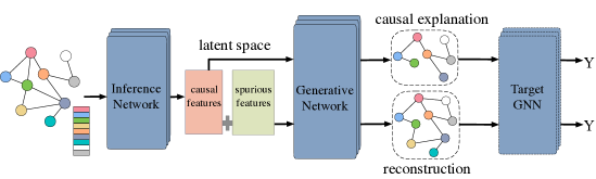
Figure 1: Illustration of OrphicX. We instantiate our explainer with a variational graph auto-encoder (VGAE), which consists of an inference network and a generative network. The causal features along with the spurious features can be used to reconstruct the graph structure within the data distribution, while the causal features are mapped to a graph-structured mask for the causal explanation. The target GNN is pre-trained, and the parameters would not be changed during the training of OrphicX.

Then we instantiate our explainer with a variational graph auto-encoder (VGAE) [8], which consists of an inference network and a generative network (shown in Figure 1). The inference network seeks a representation of the input, in which the representation is learned in such a way that a subset of the factors with large causal influence, i.e. the causal features, can be identified. The generative network is to map the causal features into an adjacency mask for the explanation. Importantly, the generative network ensures that the learned latent representations (the causal features and the spurious features together) are within the data distribution.

In a nutshell, our main contributions are highlighted as follows. We propose a new explanation technique, called OrphicX, that eXplains the predictions of any GNN by identifying the causal factors in the latent space. We utilize the notion of information flow measurements to quantify the causal information flowing from the latent features to the model predictions. We theoretically analyze the causal-effect relationships in the proposed causal model, identify a confounder, and circumvent it by leveraging the backdoor adjustment formula. We empirically demonstrate that the learned features with causal semantics are indeed informative for generating interpretable and faithful explanations for any GNNs. Our work improves model interpretability and increases trust in GNN model explanation results.

2 Method

2.1 Notations and Problem Setting

Notations. Given a pre-trained GNN (the target model to be explained), denoted as $f:\,\mathcal{G}\,\rightarrow\,\mathcal{Y}$, where $\mathcal{G}$ is the space of input graphs to the model and $\mathcal{Y}$ is the label space. Specifically, the input graph $G=(V,E)$ of the GNN includes the corresponding adjacency matrix (${\bf A}\in\mathbb{R}^{|V|\times|V|}$) and a node attribute matrix (${\bf X}\in\mathbb{R}^{|V|\times D}$). We use ${\bf Z}=[{\bf Z}_{c},{\bf Z}_{s}]\in\mathbb{R}^{|V|\times(D_{c}+D_{s})}$ to denote the latent feature matrix, where ${\bf Z}_{c}$ is the causal feature sub-matrix and ${\bf Z}_{s}$ is the spurious feature sub-matrix. Correspondingly for each node, we denote its node attribute vector by ${\bf x}$ (one row of ${\bf X}$), its causal latent features by ${\bf z}_{c}$, and its spurious latent features by ${\bf z}_{s}$.

The desiderata for GNN explanation methods. An essential criterion for explanations is fidelity [22]. A faithful explanation/subgraph should correspond to how the target GNN behaves in the vicinity of the given graph of interest. Stated differently, the outcome of feeding to the explanatory subgraph to the target GNN should be similar to that of the graph to be explained. Another essential criterion for explanations is human interpretability, which implies that the generated explanations should be sparse/compact in the context of graph-structured data [21]. In other words, a human-understandable explanation should highlight the most important part of the input while discarding the irrelevant part. In addition, an explainer should be able to explain any GNN model, commonly known as “model-agnostic” (i.e., treat the target GNN as a black box).

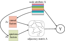
Figure 2: Illustration of the causal graph. The causal features are a set of factors in the latent space. The causal features and the spurious features together form the representation of the input graph. The graph structure is reconstructed based on the latent representation; it forms the input of the target GNN, along with the feature matrix. $y$ denotes the predicted label of the GNN target.

Problem setting. Therefore, our ultimate goal is to obtain a generative model as an explainer, denoted as $\mathcal{F}$, that can identify which part of the input causes the GNN prediction, while achieving the best possible performance under the above criteria. Consistent with prior works [34, 11, 14], we focus on explanations on graph structures. We consider the black-box setting where we do not have any information about the ground-truth labels of the input graphs and we specifically do not require access to, nor knowledge of, the process by which the target GNN produces its output. Nevertheless, we are allowed to retrieve different predictions by performing multiple queries, and we assume that the gradients of the target GNN are provided.

2.2 OrphicX

Overview. In this paper, we propose a generative model as an explainer, called OrphicX, that can generate causal explanations by identifying the causal features leading to the GNN outcome. In particular, we propose to isolate the causal features and the spurious features from the latent space. For this purpose, we first propose a causal graph to model the relationships among the causal features, the spurious features, the input graph, and the prediction of the target model. Then we show how to train OrphicX with a faithful causal-quantification mechanism based on the notion of information flow along with the backdoor adjustment formula. With the identified causal features, we are able to generate a graph-structured mask for the explanation.

Information flow for causal measurements. Recall that, our objective is to generate compact subgraphs as the explanations for the pre-trained GNN. The explanatory subgraph is causal in the sense that it tends to be independent of the spurious aspects of the input graph while holding the causal portions contributing to the prediction of the target GNN. One challenge, therefore, is how to quantify the causal influence of different data aspects in the latent space, so as to identify the portion with large causal influence, denoted by $\mathbf{Z}_{c}$. To address this issue, we leverage recent work on information-theoretic measures of causal influence [1]. Specifically, we measure the causal influence of ${\bf Z}_{c}$ on the model prediction $y$ using the information flow, denoted as $\mathbf{I}\left(\mathbf{Z}_{c}\rightarrow y\right)$, between them. Here information flow can be seen as the causal counterpart of mutual information $\mathbf{I}\left(\mathbf{Z}_{c};y\right)$.

Succinctly, our framework attempts to isolate a subset of the representation from the hidden space, denoted as $\mathbf{Z}_{c}$, such that the information flow from $\mathbf{Z}_{c}$ to $y$ is maximized. In what follows, we will show how to quantify this term corresponding to our causal model.

Causal analysis. Throughout this paper, we assume the causal model in Figure 2. Specifically, the causal features and the spurious features together form the representation of the input graph, which can be used to reconstruct the graph structure, denoted as ${\bf A}$. This ensures that the learned latent features still reflect the same data distribution as the one captured by the target GNN. The graph structure ${\bf A}$, along with the node attribute ${\bf X}$, contributes to the model prediction $y$. Stated differently, ${\bf X}$ is a confounder when we consider the cause-effect relationships between the latent features (i.e. causal features and spurious features) and the model prediction. Consequently, directly ignoring ${\bf X}$ can lead to inaccurate estimates of the causal features. To address this issue, we leverage the classic backdoor adjustment formula [20] and have:

$$P(y|do({\bf Z}_{c}))=\sum_{{\bf X}}P(y|{\bf Z}_{c},{\bf X})P({\bf X}).$$ (1)

Eqn. 1 is crucial to circumvent the confounder effect introduced by node attributes and compute the information flow $I({\bf Z}_{c}\rightarrow y)$, which is the causal counterpart of mutual information [1]. Intuitively, Eqn. 1 goes through different versions of ${\bf X}$ while keeping ${\bf Z}_{c}$ fixed to estimate the causal effect ${\bf Z}_{c}$ has on $y$. Note that $P(y|do({\bf Z}_{c}))=\sum_{{\bf X}}P(y|{\bf Z}_{c},{\bf X})P({\bf X})$ is different from $P(y|{\bf Z}_{c})=\sum_{{\bf X}}P(y|{\bf Z}_{c},{\bf X})P({\bf X}|{\bf Z}_{c})$; the former samples from the marginal distribution $P({\bf X})$, while the latter samples ${\bf X}$ from the conditional distribution $P({\bf X}|{\bf Z}_{c})$. In causal theory, $P(y|do({\bf Z}_{c}))=\sum_{{\bf X}}P(y|{\bf Z}_{c},{\bf X})P({\bf X})$ is referred to as the backdoor adjustment formula [20]. Our Theorem 2.1 below provides a way of computing the information flow $I({\bf Z}_{c}\rightarrow y)$.

Theorem 2.1 (Information flow between ${\bf Z}_{c}$ and $y$)

The information flow between the causal factors ${\bf Z}_{c}$ and the prediction $y$ can be computed as

$$I({\bf Z}_{c}\rightarrow y)$$

$$= \int_{{\bf Z}_{c}}P({\bf Z}_{c})\sum\limits_{y}P(y|do({\bf Z}_{c}))\log\frac{P(y|do({\bf Z}_{c}))}{\int_{{\bf Z}_{c}}P(y|do({\bf Z}_{c}))d{\bf Z}_{c}}d{\bf Z}_{c}$$

$$= \int_{{\bf Z}_{c}}P({\bf Z}_{c})\sum\limits_{y}\sum_{{\bf X}}P(y|{\bf Z}_{c},{\bf X})P({\bf X})\cdot$$

$$\quad\quad\log\frac{\sum_{{\bf X}}P(y|{\bf Z}_{c},{\bf X})P({\bf X})}{\int_{{\bf Z}_{c}}\sum_{{\bf X}}P(y|{\bf Z}_{c},{\bf X})P({\bf X})d{\bf Z}_{c}}d{\bf Z}_{c}$$

Note that due to the confounder ${\bf X}$, $I({\bf Z}_{c}\rightarrow y)$ is not equal to the mutual information $I({\bf Z}_{c};y)$. The term $\sum_{{\bf X}}P(y|{\bf Z}_{c},{\bf X})$ comes from Eqn. 1 and can be estimated efficiently. Specifically, we have

$$P(y|do({\bf Z}_{c}))=\sum_{{\bf X}}P(y|{\bf Z}_{c},{\bf X})P({\bf X})$$ (2)

$$=\sum_{{\bf X}}\sum_{{\bf A}}\int_{{\bf Z}_{s}}P(y|{\bf A},{\bf X})P({\bf A}|{\bf Z}_{s},{\bf Z}_{c})P({\bf Z}_{s}|{\bf Z}_{c},{\bf X})P({\bf X})d{\bf Z}_{s}$$

$$\approx\frac{1}{N_{x}N_{s}N_{z}}\sum\limits_{k=1}^{N_{x}}\sum\limits_{j=1}^{N_{s}}\sum\limits_{n=1}^{N_{z}}P(y|{\bf A}^{(kjn)},{\bf X}^{(k)}).$$ (3)

Here $k$ indexes the $N_{x}$ sampled node attribute matrices ${\bf X}^{(k)}$ from the dataset; $j$ indexes the $N_{s}$ samples for each ${\bf X}^{(k)}$, i.e., ${\bf Z}_{s}^{(kj)}\sim P({\bf Z}_{s}|{\bf Z}_{c},{\bf X}^{(k)})$; $n$ indexes the $N_{z}$ sampled graphs for each ${\bf Z}_{s}^{(kj)}$, i.e., ${\bf A}^{(kjn)}\sim p({\bf A}|{\bf Z}_{c},{\bf Z}_{s}^{(kj)})$. Note that in practice we use the variational distribution $q({\bf Z}_{s}|{\bf A},{\bf X}^{(k)})$ to approximate the true posterior distribution $P({\bf Z}_{s}|{\bf Z}_{c},{\bf X}^{(k)})$, and that in Eqn. 3, ${\bf X}$, ${\bf Z}_{c}$, and ${\bf Z}_{s}$ do not necessarily belong to the same graph in the original dataset. Intuitively this is to remove the confounding effect of ${\bf X}$ on ${\bf Z}_{c}$ and ${\bf Z}_{s}$. Consequently we have

$$\int_{{\bf Z}_{c}}P({\bf Z}_{c})P(y|do({\bf Z}_{c}))d{\bf Z}_{c}$$ (4)

$$=\int_{{\bf Z}_{c}}\sum_{{\bf X}}\sum_{{\bf A}}\int_{{\bf Z}_{s}}P(y|{\bf A},{\bf X})P({\bf A}|{\bf Z}_{s},{\bf Z}_{c})$$ (5)

$$\quad\quad\quad\quad\quad\quad\quad\quad P({\bf Z}_{s}|{\bf Z}_{c},{\bf X})P({\bf X})P({\bf Z}_{c})d{\bf Z}_{s}d{\bf Z}_{c}$$

$$\approx\frac{1}{N_{c}N_{x}N_{s}N_{z}}\sum\limits_{i=1}^{N_{c}}\sum\limits_{k=1}^{N_{x}}\sum\limits_{j=1}^{N_{s}}\sum\limits_{n=1}^{N_{z}}P(y|{\bf A}^{(ikjn)},{\bf X}^{(k)}),$$ (6)

Similarly, $i$ indexes the $N_{c}$ samples from ${\bf Z}_{c}$’s marginal distribution, i.e., ${\bf Z}_{c}^{(i)}\sim P({\bf Z}_{c})$; $k$ indexes the $N_{x}$ sampled node attribute matrices from ${\bf X}$’s marginal distribution ${\bf X}^{(k)}\sim P({\bf X})$; $j$ indexes the $N_{s}$ samples of ${\bf Z}_{s}$ for each pair $({\bf Z}_{c}^{(i)},{\bf X}^{(k)})$, i.e., ${\bf Z}_{s}^{(ikj)}\sim P({\bf Z}_{s}|{\bf Z}_{c}^{(i)},{\bf X}^{(k)})$; $n$ indexes the $N_{z}$ sampled graphs for each pair $({\bf Z}_{c}^{(i)},{\bf Z}_{s}^{(kj)})$, i.e., ${\bf A}^{(ikjn)}\sim p({\bf A}|{\bf Z}_{c}^{(i)},{\bf Z}_{s}^{(kj)})$. Note that in practice we use the variational distribution $q({\bf Z}_{s}|{\bf A},{\bf Z}_{c}^{(i)},{\bf X}^{(k)})$ to approximate the true posterior distribution $P({\bf Z}_{s}|{\bf Z}_{c}^{(i)},{\bf X}^{(k)})$.

Put together, we have

$$I({\bf Z}_{c}\rightarrow y)= \frac{1}{N_{c}N_{x}N_{s}N_{z}}\Big{[}\sum_{i=1}^{N_{c}}\sum_{y}\Big{(}\sum\limits_{k=1}^{N_{x}}\sum\limits_{j=1}^{N_{s}}\sum\limits_{n=1}^{N_{z}}P(y|{\bf A}^{(ikjn)},{\bf X}^{(k)})\Big{)}\cdot$$

$$\log\Big{(}\frac{1}{N_{x}N_{s}N_{z}}\sum\limits_{k=1}^{N_{x}}\sum\limits_{j=1}^{N_{s}}\sum\limits_{n=1}^{N_{z}}P(y|{\bf A}^{(ikjn)},{\bf X}^{(k)})\Big{)}$$

$$-\sum_{y}\Big{(}\sum\limits_{i=1}^{N_{c}}\sum\limits_{k=1}^{N_{x}}\sum\limits_{j=1}^{N_{s}}\sum\limits_{n=1}^{N_{z}}P(y|{\bf A}^{(ikjn)},{\bf X}^{(k)})\Big{)}\cdot$$

$$\log\Big{(}\frac{1}{N_{c}N_{x}N_{s}N_{z}}\sum\limits_{i=1}^{N_{c}}\sum\limits_{k=1}^{N_{x}}\sum\limits_{j=1}^{N_{s}}\sum\limits_{n=1}^{N_{z}}P(y|{\bf A}^{(ikjn)},{\bf X}^{(k)})\Big{)}\Big{]}.$$

Graph generative model as an explainer. Our framework, OrphicX, leverages the latent space of a variational graph auto-encoder (VGAE) to avoid working with input spaces with complex interdependency. Specifically, our VGAE-based framework (shown in Figure 1) consists of an inference network and a generative network. The former is instantiated with a graph convolutional encoder and the latter is a multi-layer perceptron equipped with an inner product decoder. More concretely, the inference network seeks a representation — a latent feature matrix ${\bf Z}$ of the input graph, of which the causal features ${\bf Z}_{c}$, a sub-matrix with large causal influence, can be isolated. The generative network serves two purposes: (1) it maps the causal sub-matrix into an adjacency mask, which is used as the causal explanation, and (2) it ensures that the causal features, merged with the spurious features, can reconstruct the graphs within the data distribution characterized by the target GNN.

Learning OrphicX. Learning of OrphicX can be cast as the following optimization problem:

$$\min\,\,-{I}\left(\mathbf{Z}_{c}\rightarrow y\right)+\lambda\mathcal{L}_{\mathbf{VGAE}},$$ (7)

where $\mathcal{L}_{\mathbf{VGAE}}$ is the negative evidence lower bound (ELBO) loss term that encourages the latent features ${\bf Z}$ to stay in the data manifold [8], and $\mathbf{Z}_{c}$ is the causal sub-matrix of ${\bf Z}$. A detailed description of the ELBO term of the VGAE is provided in Appendix. Our empirical results suggest that the ELBO term helps learn a sub-matrix that embeds more relevant information leading to the GNN prediction.

Recall that, our objective is to generate explanations that can provide insights into how the target GNN truly computes its predictions. An ideal explainer should fulfill the three desiderata presented in Section 2.1: high fidelity (faithful), high sparsity (compact), and model agnostic. Therefore, apart from the objective function Eqn. 7, we further enforce the fidelity and sparsity criteria through regularization specifically tailored to such explainers. Concretely, we denote the generated explanatory subgraph as $G_{c}$ and the corresponding adjacency matrix as ${\bf A}_{c}$. The sparsity criterion is measured by $\frac{||{\bf A}_{c}||_{1}}{||{\bf A}||_{1}}$, where $||\cdot||_{1}$ denotes the $l_{1}$ norm of the adjacency matrix. The fidelity criterion implies that the GNN outcome corresponding to the explanatory subgraph should be approximated to that of the target instance, i.e. $f(G_{c})\approx f(G)$, where $f(\cdot)$ is the probability distribution over the classes — the outcome of the target GNN. For this purpose, we introduce a Kullback–Leibler (KL) divergence term to measure how much the two outputs differ.

Therefore, the optimization problem can be reformulated as:

$$\min\,-I\left(\mathbf{Z}_{c}\rightarrow y\right)+\lambda_{1}\mathcal{L}_{\mathbf{VGAE}}+\lambda_{2}\frac{||{\bf A}_{c}||_{1}}{||{\bf A}||_{1}}$$

$$+\lambda_{3}\mathbf{KL}\left(f(G_{c}),f(G)\right),$$

where $\lambda_{i}$ ($i\in\{1,2,3\}$) controls the associated regularizer terms. To understand OrphicX comprehensively, a series of ablation studies for the loss function are performed. Note that, the parameters of the target GNN (shown in Figure 1) are pre-trained and would not be changed during the training of OrphicX. OrphicX only works with the model inputs and the outputs, rather than the internal structure of specific models. Therefore, our framework can be used to explain any GNN models as long as their gradients are admitted.

3 Experiments

3.1 Datasets and Settings

Datasets. We conducted experiments on benchmark datasets for interpreting GNNs: 1) For the node classification task, we evaluate different methods with synthetic datasets, including BA-shapes and Tree-cycles, where ground-truth explanations are available. We followed data processing in the literature [32]. 2) For the graph classification task, we use two datasets in bioinformatics, MUTAG [2] and NCI1 [26]. Note that the model architectures for node classification [5] and graph classification [30] tasks are different (more details of the dataset descriptions and corresponding model architectures are provided in Appendix A.2).

Comparison methods. We compare our approach against various powerful interpretability frameworks for GNNs. They are GNNExplainer [32], PGExplainer [14], and Gem [11]. Among others, PGExplainer and Gem explain the target GNN via learning an explainer. As for GNNExplainer, there is no training phase, as it is naturally designed for explaining a given instance at a time. Unless otherwise stated, we set all the hyperparameters of the baselines as reported in the corresponding papers.

Hyperparameters in OrphicX. For all datasets on different tasks, the explainers share the same model structure [8]. For the inference network, we applied a three-layer GCN with output dimensions $32$, $32$, and $16$. The generative model is equipped with a two-layer MLP and an inner product decoder. We trained the explainers using the Adam optimizer [7] with a learning rate of $0.003$ for $300$epochs. For all experiments, we set $N_{x}=5$, $N_{z}=2$, $N_{c}=25$, $N_{s}=100$, $D_{c}=3$, $\lambda_{1}=0.1$, $\lambda_{2}=0.1$, and $\lambda_{3}=0.2$. The results reported in the paper correspond to the best hyperparameter configurations. With this testing setup, our goal is to fairly compare best achievable explanation performance of the methods. Detailed implementations, including our hyperparameter search space are given in Appendix A.2.

Evaluation metrics. We evaluate our approach with two criteria. 1) Faithfulness/fidelity: are the explanations indicative of “true” model behaviors? 2) Sparsity: are the explanations compact and understandable? Below, we address these criteria, proposing quantitative metrics for evaluating fidelity and sparsity and qualitative assessment via visualizing the explanations.

To evaluate fidelity, we generate explanations for the test set according to OrphicX, Gem, PGExplainer, and GNNExplainer, respectively. We then evaluate the explanation accuracy of different methods by comparing the predicted labels of the explanatory subgraphs with the predicted labels of the input graphs using the pre-trained GNN [11]. An explanation is faithful only when the predicted label of the explanatory subgraph is the same as the corresponding input graph. To evaluate sparsity, we use different evaluation metrics. Specifically, in Mutag, the type and the size of explainable motifs are various. We measure the fraction of edges (i.e., edge ratio denoted as $R$) selected as “important” by different explanation methods for Mutag and NCI1. For the synthetic datasets, we use the number of edges (denoted as $K$), as did in prior works [11, 32]. A smaller fraction of edges or a smaller number of edges selected implies a more compact subgraph or higher sparsity.

To further check the interpretability, we use the visualized explanations to analyze the performance qualitatively. However, we do not know the ground-truth explanations for the real-world datasets. For Mutag, we ask an expert from Biochemical Engineering to label the explicit subgraph patterns as our explanation ground truth (i.e., carbon rings with chemical groups such as the azo N=N, $\textrm{NO}_{2}$ and $\textrm{NH}_{2}$ for the mutagenic class). Specifically, $739/933$ instances containing the subgraph patterns fall into the mutagenic class in the entire dataset, which corroborates that these patterns are sufficient for the ground-truth explanation. Figure 3 describes the detailed distribution of instances with various occurring subgraph patterns. With these occurring subgraph patterns, we can evaluate the explanation performance on Mutag with edge AUC. The evaluation intuition is elaborated in the  Section 3.2.

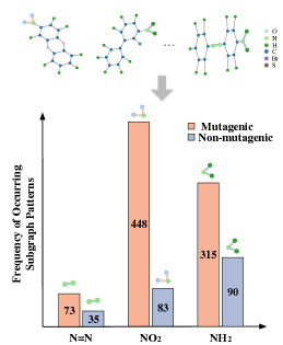
Figure 3: The frequency of occurring subgraph patterns indicates that it is reasonable to treat the labeled motifs/subgraph patterns as the explanation ground truth, i.e., carbon rings with chemical groups such as N=N, $\textrm{NO}_{2}$, and $\textrm{NH}_{2}$ for the mutagenic class.

Table 1: Explanation Accuracy on Synthetic Datasets ($\%$).

K BA-SHAPES TREE-CYCLES #of edges 5 6 7 8 9 6 7 8 9 10 OrphicX 82.4 97.1 97.1 97.1 100 85.7 91.4 100 100 100 Gem $64.7$ $94.1$ $91.2$ $91.2$ $91.2$ $74.3$ $88.6$ 100 100 100 GNNExp. $67.6$ $67.6$ $82.4$ $88.2$ $85.3$ $20.0$ $54.3$ $74.3$ $88.6$ $97.1$ PGExp. $59.5$ $59.5$ $59.5$ $59.5$ $64.3$ $76.2$ $81.5$ $91.3$ $95.4$ $97.1$

3.2 Empirical Results

Explanation performance. We first report the explanation performance for synthetic datasets and real-world datasets. In particular, we evaluate the explanation accuracy under various sparseness constraints (i.e., various $R$ for the real-world datasets and various $K$ for the synthetic datasets). Table 1 and Table 2 report the explanation accuracy of different methods specifically. A smaller number of edges (denoted as $K$) or a smaller value of edge ratio (denoted as $R$) indicates that the explanatory subgraphs are more compact. As observed, OrphicX consistently outperforms baselines across various sparseness constraints over all datasets. As the model architectures for node and graph classification [30] tasks are different, the performance corroborates that our framework is model architecture-agnostic (see the model architectures in the Appendix).

Following existing works [11, 18], we also evaluate the Log-odds difference to illustrate the fidelity of generated explanations in a more statistical view. Log-odds difference describes the resulting change in the pre-trained GNNs’ outcome by computing the difference (the initial graph and the explanation subgraph) in log odds. The detailed definition of Log-odds difference is elaborated in Appendix A.2. Figure 4 depicts the distributions of log-odds difference over the entire test set for synthetic datasets. We can observe that the log-odds difference of OrphicX is more concentrated around $0$, which indicates OrphicX can well capture the most relevant subgraphs towards the predictions by the pre-trained GNNs. As OrphicX exhibits a similar performance trend on other datasets, we present corresponding evaluation results in the Appendix.

Table 2: Explanation Accuracy on Real-World Datasets ($\%$).

R Mutag NCI1 edge ratio 0.5 0.6 0.7 0.8 0.9 0.5 0.6 0.7 0.8 0.9 OrphicX 71.4 71.2 77.2 78.8 83.2 66.9 72.7 77.1 81.3 85.4 Gem $66.4$ $67.7$ $71.4$ $76.5$ $81.8$ $61.8$ $68.6$ $70.6$ $74.9$ $83.9$ GNNExp. $65.0$ $66.6$ $66.4$ $71.0$ $78.3$ $64.2$ $65.7$ $68.6$ $75.2$ $81.8$ PGExp. $59.3$ $58.9$ $65.1$ $70.3$ $74.7$ $57.7$ $60.8$ $65.2$ $69.3$ $71.0$

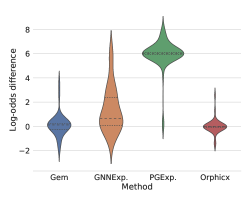
(a)

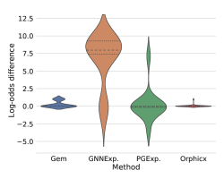
(b)

Figure 4: Explanation Performance with Log-Odds Difference. OrphicX consistently achieves the best performance overall (denser distribution around $0$ is better).

Table 3: Explanation Accuracy with Edge AUC (* means the rounded estimate of $0.9995\pm 0.0006$).

Datasets	OrphicX	Gem	GNNExp.	PGExp.	ATT
BA-SHAPES	$\mathbf{0.988\pm 0.008}$	$0.597\pm 0.001$	$0.956\pm 0.001$	$0.924\pm 0.042$	$0.815$
TREE-CYCLES	$\mathbf{0.988\pm 0.001}$	$0.761\pm 0.002$	$0.961\pm 0.003$	$0.952\pm 0.000$	$0.824$
Mutag	$\mathbf{1.000\pm 0.001}^{*}$	$0.988\pm 0.013$	$0.998\pm 0.001$	$0.998\pm 0.001$	$0.686\pm 0.098$

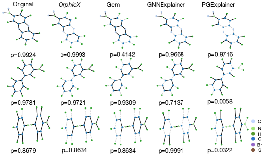
Figure 5: Explanation Visualization (MUTAG): $p$ is the corresponding probability of being classified as Mutagenic class by the pre-trained GNN. The graphs in the first column are the target instances to be explained. The solid edges in other columns are identified as ‘important’ by corresponding methods. The closer the probability to that of the target instance, the better the explanation is.

For fair comparisons, we also report the explanation fidelity of different methods in terms of edge AUC in Table 3. We follow the experimental settings of GNNExplainer and PGExplainer, where the explanation problem was formalized as a binary classification of edge. The mean and standard deviation are calculated over $5$ runs. This metric works for the datasets with ground-truth explanations (i.e., the “house”-structured pattern/motif of BA-shapes and the labeled subgraph patterns in Mutag). The intuition is that a good explanation method assigns higher weights to the edges within the ground-truth subgraphs/motifs. Regarding edge importance, one might naturally consider the self-attention mechanism as a feasible solution. Prior works have shown its performance for model explanations. For clarity, we also report the experimental results of the self-attention mechanism denoted as ATT in Table 3. The results of synthetic datasets are from GNNExplainer and PGExplainer. For Mutag, we evaluate the subgraph patterns labeled by the domain expert. As might be expected, OrphicX exhibits its superiority in identifying the most important edges captured by the pre-trained GNNs. We also observe that the prior causality-based approach, Gem, does not perform well evaluating with edge AUC. We conjecture that the explainable subgraph patterns are destroyed due to the distillation process [11]. Though the generated subgraphs with Gem can well reflect the classification pattern captured by the pre-trained GNN, it degrades the human interpretability of the generated explanations.

Explanation visualization. Figure 5 plots the visualized explanations of different methods. In particular, we focus on the visualization on Mutag, which can reflect the interpretability quantitatively and qualitatively. The first column shows the initial graphs and corresponding probabilities of being classified as “mutagenic” class by the pre-trained GNN, while the other columns report the explanation subgraphs. Associated probabilities belonging to the “mutagenic” class based on the pre-trained GNN are reported below the subgraphs. Specifically, in the first case (the first row), OrphicX can identify the essential subgraph pattern — a complete carbon ring with a $\textrm{NO}_{2}$ — leading to its label ( “mutagenic”). Nevertheless, prior works, particularly Gem, fail to recognize the explainable motif. In the second instance (the second row), OrphicX can well identify a complete carbon ring with a $\textrm{NH}_{2}$. At the same time, PGExplainer fails to recognize the $\textrm{NH}_{2}$, leading to a high probability of being classified into the wrong class — “non-mutagenic” — by the target GNN, with a probability of $0.9942$. In the third instance (the third row), a complete carbon ring with a N=N is the essential motif, consistent with the criterion from the domain expert. Overall, OrphicX can identify the explanatory subgraphs that best reflect the predictions of the pre-trained GNN. The visualization of synthetic datasets and more visualization plots on Mutag are provided in Appendix A.3.

Information flow measurements. To validate Theorem 2.1, we evaluate the information flow of the causal factors (${\bf Z}_{c}$) and the spurious factors (${\bf Z}_{s}$) corresponding to the model prediction, respectively. Figure 10(a) in Appendix A.3 shows that, as desired, the information flow from the causal factors to the model prediction is large while the information flow from the spurious factors to the prediction is small. We also evaluate the prediction performance while adding noise (mean is set as 0) to the causal factors and the spurious factors, respectively. From Table 4, we can observe that adding perturbations to the causal factors degrades the prediction performance of the pre-trained GNN significantly with the increase of the standard deviation of the noise (mean is set as 0) while adding the perturbations on the spurious counterparts does not. These insights, in turn, verify the efficacy of applying the concept of information flow for the causal influence measurements.

Table 4: Prediction Accuracy of the Pre-trained GNN on Mutag with Various Perturbation (mean is set as 0).

Perturbation std	0.0	0.3	0.5	0.8	1.0	1.3
Causal factors	$0.935$	$0.926$	$0.926$	$0.887$	$0.860$	$0.826$
Spurious factors	$0.935$	$0.936$	$0.936$	$0.935$	$0.934$	$0.926$

Ablation studies. An ablation study for the information flow in the hidden space was performed by removing the causal influence term. From Figure 10(b) in Appendix A.3, we can observe that without the causal influence term, the causal influence to the model prediction is distributed across all hidden factors. In addition, we also inspect the explanation performance for our framework as an ablation study for the loss function proposed. We empirically prove the need for different forms of regularization leveraged by the OrphicX loss function. Due to space constraints, the empirical results are provided in the Appendix.

4 Related Work

We focus on the discussions on causality-based interpretation methods. Other prior works, including GNNExplainer [32], PGExplainer [14], PGM-Explainer [25], SubgraphX [35], GraphMask [23], XGNN [34] and others [21] are provided in Appendix A.4.

Explanation essentially seeks the answers to the questions of “what if” and “why,” which are intrinsically causal. Causality, therefore, has been a plausible language for answering such questions [18, 11]. There are several viable formalisms of causality, such as structural causal models [19, 18], Granger causality [3, 11], and causal Bayesian networks [19]. While most existing works are designed for explaining conventional neural networks on image domain, Gem [11] falls into the research line of explaining graph-structural data. Specifically, Gem framed the explanation task for GNNs as a causal learning task and proposed a causal explanation model that can learn to generate compact subgraphs towards its prediction. Fundamentally, this approach monitored the response of the target GNN by perturbing the input aspects in the data space and naturally impelled the independent assumption of the explained features. Due to the interdependence property of graph-structured data and the non-linear transformation of GNNs, we argue that this assumption may reduce the efficacy and optimality of the explanation performance. Different from prior works, we quantify the causal attribution of the data aspects in the latent space, and we do not have the independent assumption of the explained features, as OrphicX is designed to generate the explanations as a whole.

Graph information bottleneck. Our work is somewhat related to the work of information bottleneck for subgraph recognition [33] but different in terms of the problem and the goals. GIB-SR [33] seeks to recognize maximally informative yet compressed subgraph given the input graph and its properties (e.g, ground truth label). On the contrary, our framework is about generating explanations to unveil the inner working of GNNs, which seeks to understand the behavior of the target model (the prediction results) rather than the ground truth labels. More concretely, the model explanation is to analyze models rather than data [16]. Moreover, our objective maximizes the causal information flowing from the latent features to the model predictions.

5 Conclusion

In this paper, we propose OrphicX, a framework for generating causal, compact, and faithful explanations for any graph neural networks. Our findings remain consistent across datasets and various graph learning tasks. Our analysis suggests that OrphicX can identify the causal semantics in the latent space of graphs via maximizing the information flow measurements. In addition, OrphicX enjoys several advantages over many powerful explanation methods: it is model-agnostic, and it does not require the knowledge of the internal structure of the target GNN, nor rely on the linear-independence assumption of the explained features. We show that causal interpretability via isolating the causal factors in the latent space offers a promising tool for explaining GNNs and mining patterns in subgraphs of graph inputs.

Explainability will promote transparency, trust, and fairness in society. It can be very helpful for graphs, including but not limited to molecular graphs, for example, visual scene graph — a graph-structured data where nodes are objects in the scene and edges are relationships between objects. Explainability can identify subgraphs relevant to a given classification, e.g., identify a scene as being indoor. In the future, additional user studies should confirm to what extent explanations in other domains (e.g., visual scene graph) provided by our OrphicX align with the needs and requirements of practitioners in real-world settings.

Potential negative impact. The privacy risks of model explanations have been empirically characterized for deep neural networks for non-relational data (with respect to graph-structured data) [24]. We conjecture that the generated explanation for GNNs may also expose private information of the training data. This will pose risks for deploying GNN-based AI systems across various domains that value model explainability and privacy the most, such as finance and healthcare.

6 Acknowledgement

The authors thank the reviewers/AC for the constructive comments to improve the paper. This project is supported by the Internal Research Fund at The Hong Kong Polytechnic University P0035763. HW is partially supported by NSF Grant IIS-2127918 and an Amazon Faculty Research Award.

Appendix A Appendix

A.1 Derivation of the Estimator in Theorem 2.1 and Eqn. 6

$$I({\bf Z}_{c}\rightarrow y) =\int_{{\bf Z}_{c}}P({\bf Z}_{c})\Big{(}\sum_{y}P(y|do({\bf Z}_{c}))\log P(y|do({\bf Z}_{c})))\Big{)}d{\bf Z}_{c}$$

$$-\sum_{y}\int_{{\bf Z}_{c}}P({\bf Z}_{c})P(y|do({\bf Z}_{c}))d{\bf Z}_{c}\cdot$$

$$\log\Big{(}\int_{{\bf Z}_{c}}P({\bf Z}_{c})P(y|do({\bf Z}_{c}))d{\bf Z}_{c}\Big{)}$$

$$= \frac{1}{N_{c}}\sum_{i=1}^{N_{c}}\sum_{y}\Big{(}\frac{1}{N_{x}N_{s}N_{z}}\sum\limits_{k=1}^{N_{x}}\sum\limits_{j=1}^{N_{s}}\sum\limits_{n=1}^{N_{z}}P(y|{\bf A}^{(ikjn)},{\bf X}^{(k)})\Big{)}\cdot$$

$$\log\Big{(}\frac{1}{N_{x}N_{s}N_{z}}\sum\limits_{k=1}^{N_{x}}\sum\limits_{j=1}^{N_{s}}\sum\limits_{n=1}^{N_{z}}P(y|{\bf A}^{(ikjn)},{\bf X}^{(k)})\Big{)}$$

$$-\sum_{y}\Big{(}\frac{1}{N_{c}N_{x}N_{s}N_{z}}\sum\limits_{i=1}^{N_{c}}\sum\limits_{k=1}^{N_{x}}\sum\limits_{j=1}^{N_{s}}\sum\limits_{n=1}^{N_{z}}P(y|{\bf A}^{(ikjn)},{\bf X}^{(k)})\Big{)}\cdot$$

$$\log\Big{(}\frac{1}{N_{c}N_{x}N_{s}N_{z}}\sum\limits_{i=1}^{N_{c}}\sum\limits_{k=1}^{N_{x}}\sum\limits_{j=1}^{N_{s}}\sum\limits_{n=1}^{N_{z}}P(y|{\bf A}^{(ikjn)},{\bf X}^{(k)})\Big{)}$$

$$= \frac{1}{N_{c}N_{x}N_{s}N_{z}}\Big{[}\sum_{i=1}^{N_{c}}\sum_{y}\Big{(}\sum\limits_{k=1}^{N_{x}}\sum\limits_{j=1}^{N_{s}}\sum\limits_{n=1}^{N_{z}}P(y|{\bf A}^{(ikjn)},{\bf X}^{(k)})\Big{)}\cdot$$

$$\log\Big{(}\frac{1}{N_{x}N_{s}N_{z}}\sum\limits_{k=1}^{N_{x}}\sum\limits_{j=1}^{N_{s}}\sum\limits_{n=1}^{N_{z}}P(y|{\bf A}^{(ikjn)},{\bf X}^{(k)})\Big{)}$$

$$-\sum_{y}\Big{(}\sum\limits_{i=1}^{N_{c}}\sum\limits_{k=1}^{N_{x}}\sum\limits_{j=1}^{N_{s}}\sum\limits_{n=1}^{N_{z}}P(y|{\bf A}^{(ikjn)},{\bf X}^{(k)})\Big{)}\cdot$$

$$\log\Big{(}\frac{1}{N_{c}N_{x}N_{s}N_{z}}\sum\limits_{i=1}^{N_{c}}\sum\limits_{k=1}^{N_{x}}\sum\limits_{j=1}^{N_{s}}\sum\limits_{n=1}^{N_{z}}P(y|{\bf A}^{(ikjn)},{\bf X}^{(k)})\Big{)}\Big{]}$$

A.2 Further Implementation Details

Datasets. BA-shapes was created with a base Barabasi-Albert (BA) graph containing $300$ nodes and $80$ five-node “house”-structured network motifs. Tree-cycles were built with a base $8$-level balanced binary tree and $80$ six-node cycle motifs. Mutag [2] and NCI1 [26] are for graph classification tasks. Specifically, Mutag contains 4337 molecule graphs, where nodes represent atoms, and edges denote chemical bonds. It contains the non-mutagenic and mutagenic class, indicating the mutagenic effects on Gram-negative bacterium Salmonella typhimurium. NCI1 consists of 4110 instances; each chemical compound screened for activity against non-small cell lung cancer or ovarian cancer cell lines. The statistics of four datasets are presented in Table 5. Note that, we report the average number of nodes and the average number of edges over all the graphs for the real-world datasets.

Table 5: Data Statistics of Four Datasets.

Datasets	BA-shapes	Tree-cycles	Mutag	NCI1
#graphs	$1$	$1$	$4,337$	$4,110$
#nodes	$700$	$871$	$29$	$30$
#edges	$4,110$	$1,950$	$30$	$32$
#labels	$4$	$2$	$2$	$2$

Table 6: Model Accuracy of Four Datasets ($\%$).

Datasets	BA-shapes	Tree-cycles	Mutag	NCI1
Accuracy	$94.1$	$97.1$	$88.5$	$78.6$

Model architectures. For classification architectures, we use the same setting as prior works [11, 32]. Specifically, for node classification, we apply three layers of GCNs with output dimensions equal to $20$ and perform concatenation to the output of three layers, followed by a linear transformation to obtain the node label. For graph classification, we employ three layers of GCNs with dimensions of $20$ and perform global max-pooling to obtain the graph representations. Then a linear transformation layer is applied to obtain the graph label. Figure 6 (a) and  6 (b) are the model architectures for node classification and graph classification, receptively.

Figure 6 (c) depicts the model architecture of OphicX for generating explanations. For the inference network, we applied a three-layer GCN with output dimensions $32$, $32$, and $16$. The generative model is equipped with a two-layer MLP and an inner product decoder. We trained the explainers using the Adam optimizer [7] with a learning rate of $0.003$ for $300$epochs. Table 7 shows the detailed data splitting for model training, testing, and validation. Note that both classification models and our explanation models use the same data splitting. See Table 8 for our hyperparameter search space. Table 6 reports the model accuracy on four datasets, which indicates that the models to be explained are performed reasonably well. Unless otherwise stated, all models, including GNN classification models and our explanation model, are implemented using PyTorch  and trained with Adam optimizer.

Table 7: Data Splitting for Four Datasets.

Datasets	#of Training	#of Testing	#of Validation
Ba-shapes	$300$	$50$	$50$
Tree-cycles	$270$	$45$	$45$
Mutag	$3,468$	$434$	$434$
NCI1	$3,031$	$410$	$411$

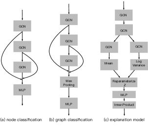
Figure 6: Model architectures.

Table 8: Hyperparameters and Ranges

Hyperparameter	Range
Causal dimension ${\bf D}_{c}$	$\{1,2,3,\cdots,8\}$
negative ELBO $\lambda_{1}$	$\{0,0.01,0.02,0.05,0.1,0.2,0.5,1\}$
Sparsity $\lambda_{2}$	$\{0,0.01,0.02,0.05,0.1,0.2,0.5,1\}$
fidelity $\lambda_{3}$	$\{0,0.01,0.02,0.05,0.1,0.2,0.5,1\}$

Negative ELBO term. The negative ELBO term is defined as Eqn. 8:

$$\mathcal{L}_{\mathbf{VGAE}}=\mathbb{E}_{q({\bf Z}|{\bf X},{\bf A})}[\log p({\bf A}|{\bf Z})]-\mathbf{KL}[q({\bf Z}|{\bf X},{\bf A})\parallel p({\bf Z})],$$ (8)

where $\mathbf{KL}[q(\cdot)\parallel p(\cdot)]$ is the Kullback-Leibler divergence between $q(\cdot)$ and $p(\cdot)$. The Gaussian prior is $p({\bf Z})=\prod_{i}p({\bf z}_{i})=\prod_{i}\mathcal{N}({\bf z}_{i}|0,\mathbf{1})$. We follow the reparameterization trick in [8] for training.

Log-odds difference. We measure the resulting change in the pre-trained GNNs’ outcome by computing the difference in log odds and investigate the distributions over the entire test set. The log-odds difference is formulated as:

$$\Delta\textrm{log-odds}=\textrm{log-odds}\left(f(G)\right)-\textrm{log-odds}\left(f(G_{c})\right)$$ (9)

where $\textrm{log-odds}(p)=\mathbf{log}\left(\frac{p}{1-p}\right)$, and $f(G)$ and $f(G_{c})$ are the outputs of the pre-trained GNN. Figure 7 depicts the distributions of log-odds difference over the entire test set for the real-world datasets.

A.3 More Experimental Results

Log-odds difference on the real-world datasets. Figure 7 depicts the distributions of log-odds difference over the entire test set for the real-world datasets. We can observe that the log-odds difference of OrphicX is more concentrated around $0$, which indicates OrphicX can well capture the most relevant subgraphs towards the predictions by the pre-trained GNNs.

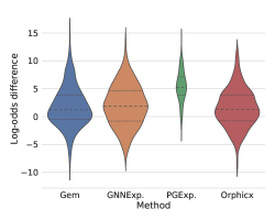
(a)

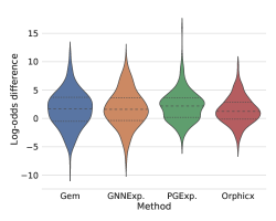
(b)

Figure 7: Explanation Performance with Log-Odds Difference. OrphicX consistently achieves the best performance overall (denser distribution around $0$ is better).

More visualization results. Figure 8 plots the visualized explanations of different methods on BA-shapes. The “house” in green is the ground-truth motif that determines the node labels. The red node is the target node to be explained. By looking at the explanations for a target node (the instance on the left side), shown in Figure 8, OrphicX can successfully identify the “house” motif that explains the node label (“middle-node” in red), when $K=6$, while GNNExplainer wrongly attributes the prediction to a node (in orange) that is out of the “house” motif. For the right one, OrphicX consistently performs well, while Gem and GNNExplainer both fail when $K=6$. Figure 9 plots more visualized explanations of different methods on Mutag.

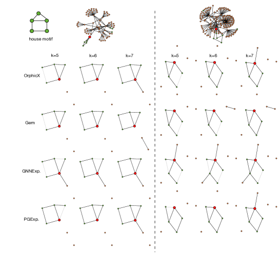
Figure 8: Explanation comparisons on BA-shapes. The “house” in green is the ground-truth motif that determines the node labels. The red node is the target node to be explained (better seen in color).

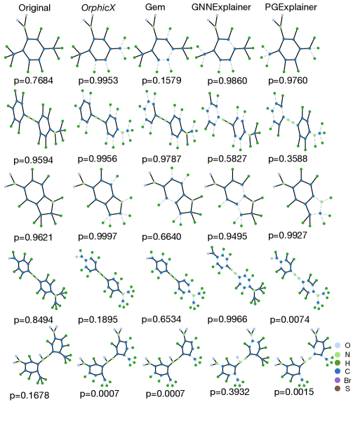
Figure 9: Explanation Visualization (MUTAG): $p$ is the corresponding probability of being classified as Mutagenic class by the pre-trained GNN. The graphs in the first column are the target instances to be explained. The solid edges in other columns are identified as ‘important’ by corresponding methods. The closer the probability to that of the target instance, the better the explanation is.

Table 9: Causal Evaluation ($\%$).

Mutag NCI1 R (edge ratio) 0.7 0.8 0.9 0.7 0.8 0.9 original $77.2$ $78.8$ $83.2$ $77.1$ $81.3$ $85.4$ deconfounder $67.1$ $71.5$ $81.5$ $71.6$ $79.2$ $87.3$

Causal evaluation. To further verify that the generated explanations are causal and therefore robust to distribution shift in the confounder (i.e., the node attributes ${\bf X}$), we construct harder versions of both datasets. Specifically, we use k-means (k=2) to split the dataset into two clusters according to the node attributes. In Mutag, we use the cluster with 3671 graph instances for explainer training and validation; we evaluate the explaining accuracy of the trained explainer on the other cluster with 665 instances. In NCI1, we use the cluster with 3197 graph instances to train an explainer, in which the training set contains 2558 instances and the validation set contains 639 instances; the explaining accuracy is evaluated with the other cluster with 906 instances. See Table 9 for details. We can observe that our approach is indeed robust to the distribution shift in the confounder.

Information flow measurements. To validate Theorem 2.1, we evaluate the information flow of the causal factors (${\bf Z}_{c}={\bf Z}[1:3]$) and the spurious factors (${\bf Z}_{s}={\bf Z}[4:16]$) corresponding to the model prediction, respectively. Figure 10(a) shows that, as desired, the information flow from the causal factors to the model prediction is large while the information flow from the spurious factors to the prediction is small.

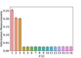
(a)

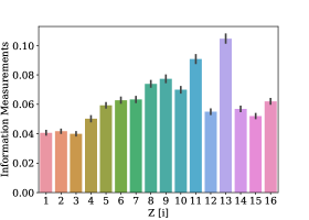
(b)

Figure 10: Information Flow Measurements. Figure 10(a) reports the information flow measurements in the hidden space, where $i$ denotes the $i$th dimension. Figure 10(b) reports the ones while the causal influence term was removed from the loss function.

Ablation study. We inspect the explanation performance for our framework as an ablation study for the loss function proposed. We empirically prove the need for different forms of regularization leveraged by the OrphicX loss function. In particular, we compute the average explanation accuracy of $3$ runs. Table 10 shows the explanation accuracy of removing a particular regularization term for Mutag and NCI1, respectively. We observe considerable performance gains from introducing the VGAE ELBO term, sparsity, and fidelity penalty. In summary, these results empirically motivate the need for different forms of regularization leveraged by the OrphicX loss function.

Table 10: Ablation Studies for Different Regularization Terms ($\%$).

Type	Causal	ELBO	Sparsity	Fidelity	Mutag	NCI1
	Influence
OrphicX	✓	✓	✓	✓	$\mathbf{0.854}$	$\mathbf{0.832}$
A	✓	✓	✓		$0.829$	$0.633$
B	✓	✓		✓	$0.804$	$0.824$
C	✓		✓	✓	$0.594$	$0.633$

Efficiency evaluation. OrphicX, Gem, and PGExplainer can explain unseen instances in the inductive setting. We measure the average inference time for these methods. As GNNExplainer explains an instance at a time, we measure its average time cost per explanation for comparisons. As reported in Table 11, we can conclude that the learning-based explainers such as OrphicX, Gem, and PGExplaienr are more efficient than GNNExplainer. These experiments were performed on an NVIDIA GTX 1080 Ti GPU with an Intel Core i7-8700K processor.

Table 11: Explanation Time of Different Methods (Per Instance (ms)).

Datasets	BA-shapes	Tree-cycles	Mutag	NCI1
OrphicX	$0.61$	$2.31$	$0.01$	$0.02$
Gem	$0.67$	$0.50$	$0.05$	$0.03$
GNNExplainer	$260.2$	$206.5$	$253.2$	$262.4$
PGExplainer	$6.9$	$6.5$	$5.5$	$5.4$

A.4 More related work on GNN interpretation

Several recent works have been proposed to provide explanations for GNNs, in which the most important features (e.g., nodes or edges or subgraphs) of an input graph are selected as the explanation to the model’s outcome. In essence, most of these methods are designed for generating input-dependent explanations. GNNExplainer [32] searches for soft masks for edges and node features to explain the predictions via mask optimization. [21] extended explainability methods designed for CNNs to GNNs. PGM-Explainer [25] adopts a probabilistic graphical model and explores the dependencies of the explained features in the form of conditional probability. SubgraphX explores the subgraphs with Monte Carlo tree search and evaluates the importance of the subgraphs with Shapley values [35]. In general, these methods explain each instance individually and can not generalize to the unseen graphs, thereby lacking a global view of the target model.

A recent study has shown that separate optimization for each instance induces hindsight bias and compromises faithfulness [23]. To this end, PGExplainer [14] was proposed to learn a mask predictor to obtain edge masks for providing instance explanations. XGNN [34] was proposed to investigate graph patterns that lead to a specific class. GraphMask [23] is specifically designed for GNN-based natural language processing tasks, where it learns an edge mask for each internal layer of the learning model. Both these approaches require access to the process by which the target model produces its predictions. As all the edges in the dataset share the same predictor, they might be able to provide a global understanding of the target GNNs. Our work falls into this line of research, as our objective is to learn an explainer that can generate compact subgraph structures contributing to the predictions for any input instances. Different from existing works, we seek faithful explanations from the language of causality [19].

References

- [1] Nihat Ay and Daniel Polani. Information Flows in Causal Networks. Advances in Complex Systems, 11(1):17–41, 2008.
- [2] Asim Kumar Debnath, Rosa L Lopez de Compadre, Gargi Debnath, Alan J Shusterman, and Corwin Hansch. Structure-Activity Relationship of Mutagenic Aromatic and Heteroaromatic Nitro Compounds. Correlation with Molecular Orbital Energies and Hydrophobicity. Journal of Medicinal Chemistry, 34(2):786–797, 1991.
- [3] Clive WJ Granger. Investigating Causal Relations by Econometric Models and Cross-Spectral Methods. Econometrica: Journal of the Econometric Society, pages 424–438, 1969.
- [4] Shantanu Gupta, Hao Wang, Zachary Lipton, and Yuyang Wang. Correcting exposure bias for link recommendation. In ICML, 2021.
- [5] Will Hamilton, Zhitao Ying, and Jure Leskovec. Inductive Representation Learning on Large Graphs. In Proc. Advances in Neural Information Processing Systems, 2017.
- [6] Hengguan Huang, Fuzhao Xue, Hao Wang, and Ye Wang. Deep Graph Random Process for Relational-Thinking-Based Speech Recognition. In ICML, 2020.
- [7] Diederik P Kingma and Jimmy Ba. Adam: A Method for Stochastic Optimization. In Proc. International Conference for Learning Representations, 2015.
- [8] Thomas N Kipf and Max Welling. Variational Graph Auto-Encoders. In Proc. NIPS Bayesian Deep Learning Workshop, 2016.
- [9] Wanyu Lin, Zhaolin Gao, and Baochun Li. Guardian: Evaluating Trust in Online Social Networks with Graph Convolutional Networks. In Proc. IEEE International Conference on Computer Communications, 2020.
- [10] Wanyu Lin, Zhaolin Gao, and Baochun Li. Shoestring: Graph-based Semi-Supervised Classification with Severely Limited Labeled Data. In Proceedings of the IEEE/CVF Conference on Computer Vision and Pattern Recognition, pages 4174–4182, 2020.
- [11] Wanyu Lin, Hao Lan, and Baochun Li. Generative Causal Explanations for Graph Neural Networks. In Proc. International Conference on Machine Learning, 2021.
- [12] Wanyu Lin and Baochun Li. Medley: Predicting Social Trust in Time-Varying Online Social Networks. In Proc. IEEE International Conference on Computer Communications, 2021.
- [13] Scott M Lundberg and Su-In Lee. A Unified Approach to Interpreting Model Predictions. In Proc. Advances in Neural Information Processing Systems, pages 4765–4774, 2017.
- [14] Dongsheng Luo, Wei Cheng, Dongkuan Xu, Wenchao Yu, Bo Zong, Haifeng Chen, and Xiang Zhang. Parameterized Explainer for Graph Neural Network. In Proc. Advances in Neural Information Processing Systems, 2020.
- [15] Chengzhi Mao, Amogh Gupta, Augustine Cha, Hao Wang, Junfeng Yang, and Carl Vondrick. Generative Interventions for Causal Learning. In CVPR, 2021.
- [16] Christoph Molnar. Interpretable Machine Learning. Lulu. com, 2020.
- [17] Federico Monti, Davide Boscaini, Jonathan Masci, Emanuele Rodola, Jan Svoboda, and Michael M Bronstein. Geometric Deep Learning on Graphs and Manifolds using Mixture Model CNNs. In Proc. IEEE Conference on Computer Vision and Pattern Recognition, pages 5115–5124, 2017.
- [18] Matthew O Shaughnessy, Gregory Canal, Marissa Connor, Mark Davenport, and Christopher Rozell. Generative Causal Explanations of Black-Box Classifiers. In Proc. Advances in Neural Information Processing Systems, 2020.
- [19] Judea Pearl. Causality. Cambridge University Press, 2009.
- [20] Judea Pearl, Madelyn Glymour, and Nicholas P Jewell. Causal Inference in Statistics: A Primer. John Wiley & Sons, 2016.
- [21] Phillip E Pope, Soheil Kolouri, Mohammad Rostami, Charles E Martin, and Heiko Hoffmann. Explainability Methods for Graph Convolutional Neural networks. In Proc. IEEE Conference on Computer Vision and Pattern Recognition, pages 10772–10781, 2019.
- [22] Marco Tulio Ribeiro, Sameer Singh, and Carlos Guestrin. “Why Should I Trust You?”: Explaining the Predictions of Any Classifier. In Proc. SIGKDD. ACM, 2016.
- [23] Michael Sejr Schlichtkrull, Nicola De Cao, and Ivan Titov. Interpreting Graph Neural Networks for {NLP} With Differentiable Edge Masking. In International Conference on Learning Representations, 2021.
- [24] Reza Shokri, Martin Strobel, and Yair Zick. On the Privacy Risks of Model Explanations. In Proc. AAAI/ACM Conference on AI, Ethics, and Society, pages 231–241, 2021.
- [25] Minh N Vu and My T Thai. PGM-Explainer: Probabilistic Graphical Model Explanations for Graph Neural Networks. In Proc. Advances in Neural Information Processing Systems, 2020.
- [26] Nikil Wale, Ian A Watson, and George Karypis. Comparison of Descriptor Spaces for Chemical Compound Retrieval and Classification. Knowledge and Information Systems, 14(3):347–375, 2008.
- [27] Hao Wang and Wu-Jun Li. Online Egocentric Models for Citation Networks. In IJCAI, 2013.
- [28] Hao Wang, Xingjian Shi, and Dit-Yan Yeung. Relational Deep Learning: A Deep Latent Variable Model for Link Prediction. In AAAI, pages 2688–2694, 2017.
- [29] Yuhao Wang, Vlado Menkovski, Hao Wang, Xin Du, and Mykola Pechenizkiy. Causal Discovery from Incomplete Data: A Deep Learning Approach. 2020.
- [30] Keyulu Xu, Weihua Hu, Jure Leskovec, and Stefanie Jegelka. How Powerful are Graph Neural Networks? In International Conference on Learning Representations, 2018.
- [31] Zihao Xu, Guang-He Lee, Yuyang Wang, Hao Wang, et al. Graph-Relational Domain Adaptation. ICLR, 2022.
- [32] Zhitao Ying, Dylan Bourgeois, Jiaxuan You, Marinka Zitnik, and Jure Leskovec. GNNExplainer: Generating Explanations for Graph Neural Networks. In Proc. Advances in Neural Information Processing Systems, pages 9244–9255, 2019.
- [33] Junchi Yu, Tingyang Xu, Yu Rong, Yatao Bian, Junzhou Huang, and Ran He. Graph Information Bottleneck for Subgraph Recognition. In International Conference on Learning Representations, 2021.
- [34] Hao Yuan, Jiliang Tang, Xia Hu, and Shuiwang Ji. XGNN: Towards Model-Level Explanations of Graph Neural Networks. In Proc. SIGKDD. ACM, 2020.
- [35] Hao Yuan, Haiyang Yu, Jie Wang, Kang Li, and Shuiwang Ji. On Explainability of Graph Neural Networks via Subgraph Explorations. In Proc. International Conference on Machine Learning, 2021.
- [36] Yuan Yuan, Xiaodan Liang, Xiaolong Wang, Dit-Yan Yeung, and Abhinav Gupta. Temporal Dynamic Graph LSTM for Action-driven Video Object Detection. In ICCV, 2017.