Noise assisted quantum coherence protection in hierarchical environment

Abstract

In this paper, we investigate coherence protection of a quantum system coupled to a hierarchical environment by utilizing noise. As an example, we solve the Jaynes-Cummings (J-C) model in presence of both a classical and a quantized noise. The master equation is derived beyond the Markov approximation, where the influence of memory effects from both noises is taken into account. More importantly, we find that the performance of the coherence protection sensitively depends on the non-Markovian properties of both noises. By analyzing the mathematical mechanism of the coherence protection, we show the decoherence caused by a non-Markovian noise with longer memory time can be suppressed by another Markovian noise with shorter memory time. Last but not least, as an outlook, we try to analyze the connection between the atom-cavity entanglement and the atomic coherence, then discuss the possible clue to search the required noise. The results presented in this paper show the possibility of protecting coherence by utilizing noise and may open a new path to design noise-assisted coherence protection schemes.

I Introduction

Quantum coherence is a unique feature that makes the quantum realm to be different from the classical world Zurek (2003). It is also a precious resource in quantum computation. Particularly, more research has focused on quantum coherence since the quantum computational advantage has been observed in experiments Arute et al. (2019); Zhong et al. (2020). However, quantum coherence is fragile when the quantum system inevitably interacts with its environment Zurek (1991); Yu and Eberly (2004, 2009). To protect quantum coherence, various smart schemes are proposed to eliminate the decoherence caused by noises. For example, quantum error correction codes Shor (1995); Steane (1996); Bennett et al. (1996); Webster (2020); Fowler et al. (2012) is a direct analog to the classical error correction, where auxiliary qubits are employed as redundancy. Besides, one can also cancel the decoherence by inserting control pulses periodically, which dates back to the spin-echo technique and extends to a family of dynamical decoupling schemes Hahn (1950); Uhrig (2007); Viola and Lloyd (1998); Viola et al. (1999); Khodjasteh and Lidar (2005). Another widely studied scheme is the quantum feedback control Wiseman and Milburn (1993); Wiseman (1994); Zhang et al. (2017); Geremia (2004), in which one can monitor the decoherence process and use feedback operations to compensate the loss of coherence. Certainly, there are several other ways to fight against noise, such as decoherence free space, quantum weak measurement reversal Koashi and Ueda (1999); Korotkov and Jordan (2006); Korotkov and Keane (2010); Ashhab and Nori (2010), environmental-assisted error correction Nagali et al. (2009); Trendelkamp-Schroer et al. (2011); Gregoratti and Werner (2003); Wang et al. (2014), etc. However, all these methods have their own limitations and the implementation of these schemes requires extra physical resources. Particularly, when multiple noises appear, more resources (more redundancy qubits, multiple layers of control pulses, extra feedback loops, or a larger decoherence-free space, etc.) are required to eliminate all noises.

In contrast to active coherence protection schemes discussed above, it is also valuable to investigate the properties of noise and its impact on decoherence Clerk et al. (2010). Particularly, in the presence of multiple noises, it is interesting to ask whether the decoherence caused by a noise can be eliminated by another noise. This may imply an alternative way to weaken the decoherence of quantum system purely by utilizing the properties of noises Corn and Yu (2009); Jing and Wu (2013), which is certainly beneficial for the potential error correction operations in the next step. A few successful examples have been shown in Refs. Jing and Wu (2013); Jing et al. (2014, 2018); Khodorkovsky et al. (2008), although the research in this direction is still limited. Two questions have to be answered. (i) In what configuration, adding a noise can weaken the decoherence caused by another noise, namely for a given noise, how to add a second noise to reduce the decoherence. (ii) What are the impacts of the properties (e.g., the memory time) of the two noises. Particularly, whether the non-Markovian properties are helpful to reduce the decoherence.

In this paper, we try to find some clues to answer these two questions by analyzing the decoherence of a particular physical model, a quantum system coupled to a hierarchical environment as shown in Fig. 1 (a). Besides the quantized noise from the bath $H_{{\rm B}}$, a second noise $\xi(t)$ or $\eta(t)$ is introduced to reduce the decoherence. First of all, we derive the master equation beyond the Markov approximation in presence of both noises, which ensures an accurate evolution taking non-Markovian memory effects into account. The derivation of time-convolutionless master equation (with both classical and quantized noises) itself is valuable in theoretical studies. This may provide a systematic way to derive master equations and study the mutual (indirect) interactions of two noises in the future. Second, as the central results of the paper, we show the decoherence sensitively depends on the properties of both noises (one is from the quantized bosonic bath, the other is the classical noise). In particular, the non-Markovian properties like the memory time of the two noises directly determine that adding a second noise leads to a positive or negative effect of coherence protection. This partially answers the question (ii) and emphasizes the importance of non-Markovian behaviors Zhao et al. (2011); Zhao (2019); Mu et al. (2016). Third, we also analyze the performance of the coherence protection for different noises, $\xi(t)$ or $\eta(t)$. In a brief summary, the mechanism of the coherence protection can be mathematically interpreted as the contribution of a slow-varying function can be eliminated by a fast-varying function in the time-integral. Therefore, it may imply the possibility of using a high-frequency noise to suppress a low-frequency noise. Last but not least, as an outlook, we briefly discuss the relation between decoherence and the entanglement generation between the system and the “pseudo-environment”. This may provide useful clues to answer the question (i). At least, it provides a possible direction to search what type of a second noise can protect the coherence.

The rest of the paper is organized as follows: In Sec. II, we illustrate our coherence protection scheme in an example model and solve the model beyond the Markov approximation. Non-Markovian master equations are derived in presence of both classical and quantized noises. In Sec. III, we show the coherence can be protected by adding another noise and analyze how the properties of the two noises affect the performance of the coherence protection. In Sec. IV, we draw a conclusion and discuss several valuable research topics in the future.

Figure 1: (a) Schematic diagram of a quantum system coupled to a hierarchical environment. (b) An example of pseudo-environment: J-C model coupled to an external bath. The atom can be regarded as the quantum system and the cavity plays the role of pseudo-environment. The coupling strength between atom and cavity (pseudo-environment) depends on the position of the atom in the cavity Natali and Ficek (2007); Wu and Yang (1997); Mabuchi et al. (1999); Duan et al. (2003); Hood et al. (2000).

II Model and solution

II.1 The model: hierarchical environment

In order to illustrate the feasibility of using noise to suppress decoherence caused by another noise, we focus on a common scenario that a quantum system is coupled to a hierarchical environment as shown in Fig. 1 (a). Similar to Ref. Qiao et al. (2019), an artificial quantum system $H_{{\rm E}}$ is introduced as a “pseudo-environment” to connect the system $H_{{\rm S}}$ and the bath $H_{{\rm B}}$. The reason to consider such a “pseudo-environment” is that the coupling between $H_{{\rm S}}$ and $H_{{\rm E}}$ is typically easier to be manipulated (e.g., adding a noise) than the direct coupling to $H_{{\rm B}}$. In this scenario, $H_{{\rm E}}+H_{{\rm int}}+H_{{\rm B}}$ is regarded as a hierarchical environment of $H_{{\rm S}}$. The randomness of the bath can be regarded as a quantum noise, resulting a coherence loss when taking the trace of environmental degrees of freedom Zurek (2003, 1991); Gardiner and Zoller (2004). Besides, we also consider a second noise originates from the fluctuation of the classical fields. Here, we focus on two types. On is noise $\xi(t)$ in the coupling $G$ between $H_{{\rm S}}$ and $H_{{\rm E}}$ and the other is noise $\eta(t)$ directely coupled to the system.

For different physical system the dominant noise could be very different. In the following sections, we will discuss the impacts of both types of noises. In Sec.III, we mainly focus on the noise $\xi(t)$ with a detailed discussion on the influence of its non-Markovian properties. In Sec.III.4, we make a brief discussion on the noise $\eta(t)$ and its difference from $\xi(t)$.

The hierarchical environment configuration in Fig. 1 (a) is very common in many physical systems. One example in cavity-QED Rempe et al. (1987); Eberly et al. (1980); Hood et al. (2000); Natali and Ficek (2007); Zheng and Guo (2000) system is given in Fig. 1 (b). It can be described by the Jaynes-Cummings (J-C) model Jaynes and Cummings (1963) coupled to an external environment. The Hamiltonian can be written as

$$H_{\mathrm{tot}}=H_{{\rm JC}}+H_{\mathrm{B}}+H_{\mathrm{int}},$$ (1)

where

$$H_{{\rm JC}}=\frac{\omega(t)}{2}\sigma_{z}+\Omega a^{\dagger}a+G(t)a\sigma_{+}+G(t)a^{\dagger}\sigma_{-},$$ (2)

$$H_{\mathrm{B}}=\sum_{i}\omega_{i}b^{\dagger}b_{i},$$ (3)

$$H_{\mathrm{int}}=\sum_{i}g_{i}(ab_{i}^{\dagger}+a^{\dagger}b_{i}).$$ (4)

In Eq. (2), $H_{{\rm JC}}$ is the J-C Hamiltonian Shore and Knight (1993); Jaynes and Cummings (1963); Rempe et al. (1987) describing the interaction between a two-level atom and a cavity, where $a$ is the annihilation operator of the cavity mode with frequency $\Omega$, $\sigma_{z}=|e\rangle\langle e|-|g\rangle\langle g|$, $\sigma_{+}=|e\rangle\langle g|$, and $\sigma_{-}=|g\rangle\langle e|$ are the atomic operators. The cavity leakage is described by an interaction $H_{\mathrm{int}}$ in Eq. (4) with the external bosonic bath $H_{\mathrm{B}}$ in Eq. (3), where $b_{i}$ are the annihilation operators of different modes in the bath. The cavity plus the external bath can be regarded as a hierarchical environment, and the cavity plays a role of pseudo-environment ($H_{{\rm S}}=\frac{\omega}{2}\sigma_{z}$, $H_{{\rm E}}=\Omega a^{\dagger}a$).

Besides the cavity-QED example shown in Fig. 1 (b), there may be other physical realizations of the Hamiltonian (2). For example, in the circuit-QED system Devoret and Schoelkopf (2013), such a Hamiltonian can be used to describe the interaction between artificial atoms You and Nori (2005, 2011); Kastner (1993) and quantum harmonic oscillators. Besides, when the semiconductor quantum dots are coupled to a cavity in recent the experimental progress Burkard et al. (2020), the system can be also described by the J-C model Burkard et al. (2020). A detailed discussion on alternative physical system of J-C models is given in Appendix A.

It is also worth to note that the J-C model is not the only example of a hierarchical environment. In solid state quantum dots Hanson et al. (2007), the electron spin degree of freedom is naturally coupled to the outside environment through the spin-orbit interaction Bychkov and Rashba (1984); Dresselhaus (1955), where the orbital degree of freedom naturally plays the role of the pseudo-environment. One particular example is also discussed in Appendix A.

The key point of achieving coherence protection by using noise is the time dependent coupling $G(t)$ and frequency $\omega(t)$, however, in different physical system, the realizations of the noises are also different. For example, in the cavity-QED system shown in Fig. 1 (b), the noise in $G(t)$ may originates from the motion of the atom in the cavity. If the atom is near the anti-node or the node of the standing wave in the cavity, the coupling strength may be quite different Natali and Ficek (2007); Wu and Yang (1997); Mabuchi et al. (1999); Duan et al. (2003); Hood et al. (2000). Only considering the $x$-component freedom, it can be written as Wu and Yang (1997); Mabuchi et al. (1999)

$$G(t)=G_{0}\sin\left\{k\left[x_{0}+\xi(t)\right]\right\},$$ (5)

where $k$ is the wave number of the standing wave and $x(t)=x_{0}+\xi(t)$ is the position of the atom in $x$-direction. Suppose the atom moves in the cavity randomly, the function $x(t)$ can be described by a stochastic process (e.g., vibration or Brownian motion of the atom). In contrast, in the circuit-QED system discussed in Appendix A, The tunable (time-dependent) coupling can be realized by electrical signals (through external flux of the coupler) Tian et al. (2008). Some other tunable coupling schemes such like flux qubit coupled to a resonator are also discussed in Refs. van den Brink et al. (2005); Averin and Bruder (2003); Plourde et al. (2004); Hime et al. (2006). Therefore, the noise introduced in the coupling can be either noise in natural world like the Brownian motion of an atom or some artificial noises like random electrical pulses.

The randomness in $\omega(t)$ is widely studied in circuit-QED system Kjaergaard et al. (2020); You and Nori (2005, 2011), and it often originates from the charge noise. In the example discussed in Appendix A, the fluctuation of magnetic field can also cause time-dependent $\omega(t)$ Burkard et al. (2020); Hanson et al. (2007). Here, we assume

$$\omega(t)=\omega_{0}+\eta(t),$$ (6)

where the stochastic function $\eta(t)$ represents the noise.

In this paper, we only assume there is one type of classical noise, either $\xi(t)$ or $\eta(t)$ is applied. By following the same procedure in Appendix B, one can certainly solve the case both $\xi(t)$ and $\eta(t)$ are non-zero, but it is left for the future studies.

II.2 Solution

Despite the coherence protection we will discuss in the following sections, the solution of this model itself is also valuable since the model attracts so much research interests in theoretical and experimental studies O’Connell et al. (2010); Mi et al. (2018); Chen et al. (2021, 2017a, 2020); Zhao et al. (2020); Xiong et al. (2019); Chen et al. (2017b). For instance, a better understanding of this model may contribute to solving the non-Markovian measurement problem which can be applied in gravitational wave detection Chen (2013); Yang et al. (2012). However, previous studies Breuer and Petruccione (2007) are often based on Markov approximation. In this paper, we employ the “non-Markovian quantum state diffusion” (NMQSD) approach to derive a fundamental dynamic equation of the system. Then, we obtain the master equation by taking the statistical mean over all noises. The master equation simultaneously contains the impacts from two noises, $\xi(t)$ [or $\eta(t)$] plus the noise from $H_{{\rm B}}$. It provides a powerful tool to investigate the non-Markovian dynamics under the influences of both the classical noise and the quantized noise.

By expanding the environmental degrees of freedom with the multi-mode Bargemann state $|z\rangle\equiv\prod_{i}|z_{i}\rangle$, one can define a stochastic state vector $|\psi_{t}\rangle\equiv\langle z|\psi_{{\rm tot}}\rangle$. Noticing the total state vector $|\psi_{{\rm tot}}\rangle$ satisfies the Schrödinger equation, one can obtain the dynamic equation for $|\psi_{t}\rangle$ as

$$\frac{\partial}{\partial t}|\psi_{t}\rangle=\left[-iH_{{\rm JC}}+az_{t}^{\ast}-a^{\dagger}\int\nolimits_{0}^{t}ds\alpha(t,s)\frac{\delta}{\delta z_{s}^{\ast}}\right]|\psi_{t}\rangle,$$ (7)

called the NMQSD equation Diosi et al. (1998); Strunz et al. (1999); Yu et al. (1999). Equation (7) is obviously a stochastic differential equation whose solution $|\psi_{t}\rangle$ depends on two stochastic variables. One is the classical noise represented by stochastic function $\xi(t)$ or $\eta(t)$ in $H_{{\rm JC}}$, the other is the noise from the quantized bath represented by the noise function $z_{t}^{\ast}=-i\sum_{i}g_{i}z_{i}^{\ast}e^{i\omega_{i}t}$. The statistical properties of these two types of noises can be characterized by their correlation functions

$$M\{z_{t}\} = M\{z_{t}z_{s}\}=0,$$

$$M\{z_{t}z_{s}^{*}\} = \langle\hat{B}^{\dagger}(t)B(s)\rangle=\alpha_{1}(t,s),$$ (8)

$$\langle\xi(t)\rangle=0 ,\quad\langle\xi(t)\xi(s)\rangle=\alpha_{2}(t,s),$$ (9)

$$\langle\eta(t)\rangle=0 ,\quad\langle\eta(t)\eta(s)\rangle=\alpha_{3}(t,s),$$ (10)

where $M\{\cdot\}\equiv\int\frac{dz^{2}}{\pi}e^{-|z|^{2}}\{\cdot\}$ denotes the statistical mean over the noise $z_{t}^{*}$ and $\langle\cdot\rangle$ denotes the statistical mean over the classical noises ($\xi$ or $\eta$). The bath operator $\hat{B}(t)$ is defined as $\hat{B}(t)=\sum_{i}g_{i}b_{i}e^{-i\omega_{i}t}$. Since the degrees of freedom of the bath is huge, the time dependent operator $\hat{B}(t)$ can be regarded as a source randomness and its statistical properties is governed by $\langle\hat{B}^{\dagger}(t)B(s)\rangle=\alpha_{1}(t,s)$. The properties of these two correlation functions $\alpha_{1}(t,s)$ and $\alpha_{2}(t,s)$ [or $\alpha_{3}(t,s)$] may substantially affect the decoherence process, we will discuss their impacts in Sec. III and Sec. III.4 in details.

It is worth to note that Eq. (7) is directly derived from the microscopic Hamiltonian without any approximation. All the effects (particularly the non-Markovian effects, measured by e.g., non-Markovianity Breuer et al. (2009)) in the dynamics will be captured by this equation.

The key point of solving Eq. (7) is replacing the functional derivative $\frac{\delta}{\delta z_{s}^{\ast}}$ by a time-dependent operator $O(t,s,z^{*})$ defined by $\frac{\delta}{\delta z_{s}^{\ast}}|\psi_{t}\rangle\equiv O(t,s,z^{*})|\psi_{t}\rangle$, so that Eq. (7) can be rewritten as

$$\frac{\partial}{\partial t}|\psi_{t}\rangle =H_{{\rm eff}}|\psi_{t}\rangle,$$ (11)

$$H_{{\rm eff}} =-iH_{\mathrm{JC}}+az_{t}^{\ast}-a^{\dagger}\bar{O}(t,z^{*}),$$ (12)

where $\bar{O}(t,z^{*})=\int_{0}^{t}\alpha(t,s)O(t,s,z^{*})ds$. The operator $O$ can be determined from the consistency condition $\frac{\delta}{\delta z_{s}^{\ast}}\frac{\partial}{\partial t}|\psi_{t}\rangle=\frac{\partial}{\partial t}\frac{\delta}{\delta z_{s}^{\ast}}|\psi_{t}\rangle$ (see Appendix B). Then, one can solve Eq. (11) with a single realization of the noises $\xi(t)$ [or $\eta(t)$] and $z_{t}^{*}$ to obtain a particular trajectory of the evolution. However, the density matrix of the atom-cavity system must be reconstructed by taking the two-fold ensemble average over many realizations of the stochastic state vector $|\psi_{t}\rangle$, i.e.,

$$\rho=\left\langle M\left\{|\psi_{t}\rangle\langle\psi_{t}|\right\}\right\rangle.$$ (13)

Here, the statistical mean $M\{\cdot\}$ (over $z_{t}^{*}$) and $\langle\cdot\rangle$ [over $\eta(t)$ or $\xi(t)]$ can be numerically obtained by averaging over thousands of trajectories. Alternatively, one can also derive a master equation by using the Novikov theorem Yu et al. (1999). For example, in the case $\xi(t)=0$ is a constant, i.e., only the classical noise $\eta(t)$ is applied, the master equation can be derived as (for details, see Appendix B),

$$\frac{d}{dt}\rho=-i\left[H_{{\rm 0}},\rho\right]+\left\{\left[a,\rho\bar{O}^{\dagger}\right]+\left[\sigma_{z},\rho\bar{D}^{\dagger}\right]+{\rm h.c.}\right\},$$ (14)

where $H_{0}=\frac{\omega_{0}}{2}\sigma_{z}+\Omega a^{\dagger}a+G_{0}\sin(kx_{0})(a\sigma_{+}+a^{\dagger}\sigma_{-})$, the operator $\bar{D}$ is defined as $\bar{D}=i\int_{0}^{t}ds\alpha_{3}(t,s)\frac{\delta}{\delta\eta(s)}\equiv i\int_{0}^{t}ds\alpha_{3}(t,s)D(t,s,\eta)$ with the boundary condition $D(t,s=t,\eta)=\sigma_{z}$.

According to the consistency conditions $\frac{\delta}{\delta z_{s}^{\ast}}\frac{\partial}{\partial t}|\psi_{t}\rangle=\frac{\partial}{\partial t}\frac{\delta}{\delta z_{s}^{\ast}}|\psi_{t}\rangle$ and $\frac{\delta}{\delta\eta(s)}\frac{\partial}{\partial t}|\psi_{t}\rangle=\frac{\partial}{\partial t}\frac{\delta}{\delta\eta(s)}|\psi_{t}\rangle$, one can obtain the operators $O$ and $D$ will satisfy the equations

$$\frac{d}{dt}D=\left[H_{{\rm eff}},D\right]+\frac{\delta}{\delta\eta(s)}H_{{\rm eff}},$$ (15)

$$\frac{d}{dt}O=\left[H_{{\rm eff}},O\right]+a^{\dagger}\frac{\delta}{\delta z_{s}^{*}}\bar{O},$$ (16)

with the boundary conditions $D(t=s,s,\eta)=-i\frac{1}{2}\sigma_{z}$ and $O(t=s,s,z^{*})=a$. From Eqs. (15) and (16), the operator $D$, representing the impact from noise $\eta(t)$, depends on the $z_{t}^{*}$ term in $H_{{\rm eff}}$. In the same way, the operator $O$, representing the impact from noise $z_{t}^{*}$ also depends on the $\eta(t)$ term. As a result, although the master equation (14) is formally written as the summation of two Lindblad super-operators, it does not mean the combined effect of two noises is simply the summation of the impacts from two individual noises. Physically, although the two noises are not correlated, they can still affect each other through quantum system $H_{{\rm S}}$ if non-Markovian feedback effects exist. Therefore, the master equation (14) provides a powerful tool to study the influence of one noise on the other noise. However, it is not the central topic of this paper and will be left for a future study.

Equations (15) and (16) can be numerically solved with iteration method Suess et al. (2014), or the operators $O$ and $D$ can be analytically expend into series by the order of noises up to on-demand accuracy Yu et al. (1999); Li et al. (2014); Xu et al. (2014). Here, we use a simple example to show how the master equation is reduced to the standard Lindblad master equation with constant rate of decoherence. In the Markovian case, the correlation functions become $\delta$-functions as $\alpha_{1}(t,s)=\Gamma_{1}\delta(t,s)$ and $\alpha_{3}(t,s)=\Gamma_{3}\delta(t,s)$. Then, one can obtain $\bar{O}^{\dagger}=\frac{\Gamma_{1}}{2}a^{\dagger}$ and $\bar{D}=\frac{\Gamma_{3}}{2}\sigma_{z}$ from the boundary conditions (boundary values of $O$ and $D$ are selected by the $\delta$-functions). Therefore, the master equation in Eq. (14) will be reduced to the Markovian master equation in the standard Lindblad form as

$$\frac{d}{dt}\rho=-i\left[H_{{\rm 0}},\rho\right]+\left\{\frac{\Gamma_{1}}{2}\left[a,\rho a^{\dagger}\right]+\frac{\Gamma_{3}}{2}\left[\sigma_{z},\rho\sigma_{z}\right]+{\rm h.c.}\right\},$$ (17)

The first and second Lindblad terms represent the amplitude and phase damping of the atom respectively Gardiner and Zoller (2004).

In a more general case with arbitrary correlation functions, the operators $O$ and $D$ are in more complicated forms Zhao et al. (2017, 2011); Yu et al. (1999); Zhao (2019); Zhao et al. (2013). It is worth to note that in order to obtain a compact form of the master equation (14), we have assumed that both $\bar{O}$ and $\bar{D}$ are noise-independent operators. The general form of the master equation is derived in Appendix B. Nevertheless, it is verified in Appendix B.3 that the noise term is indeed much smaller than other terms. So, it is reasonable to approximately neglect the noise-dependent part in operators $\bar{O}$ and $\bar{D}$ to obtain a master equation in the from of Eq. (14).

Similarly, in the case $\eta(t)=0$, i.e., only the classical noise $\xi(t)$ is applied, one can also derive a master equation as

$$\frac{d}{dt}\rho=-i\left[H_{{\rm 0}}^{\prime},\rho\right]+\left\{\left[a,\rho\bar{O}^{\dagger}\right]+\left[V,\rho\bar{D}_{G}^{\dagger}\right]+{\rm h.c.}\right\},$$ (18)

where $H_{0}^{\prime}=\frac{\omega_{0}}{2}\sigma_{z}+\Omega a^{\dagger}a$, $V=a\sigma_{+}+a^{\dagger}\sigma_{-}$, and $\bar{D}_{G}=i\int_{0}^{t}ds\left\langle G(t)G(s)\right\rangle D_{G}(t,s,G)=i\int_{0}^{t}ds\left\langle G(t)G(s)\right\rangle\frac{\delta}{\delta G(s)}$ with the boundary condition $D_{G}(t,s=t,G)=V$. The detailed derivation is shown in Appendix B. Equations (14) and (18) formally contain no convolution terms, but the operators $O$, $D$, and $D_{G}$ include the time integration over time, which represents the impacts from the history (non-Markovian effects). These master equations are derived beyond the Markovian approximation, thus applicable to either non-Markovian case or Markovian case. When taking the Markov-limit, our equation is reduced to Markovian equation as shown in Eq. (17). However, in non-Markovian case, they are still valid.

For computational purpose, Eq. (11) requires the two-fold statistical mean over many trajectories. However, the resource to store the pure state $|\psi_{t}\rangle$ ($\propto N$, $N$ is the dimension of the Hilbert space) is less than the resource to store the density operator $\rho$ ($\propto N^{2}$). Therefore, when $N$ is large, the NMQSD equation has a computational advantage comparing to the master equation Eq. (14) or Eq. (18). In this paper, we average the quantum noise $z_{t}^{*}$ by using the Novikov theorem Yu et al. (1999), and obtain a statistical master equation as

$$\frac{d}{dt}\rho^{\prime}=-i\left[H_{{\rm JC}},\rho^{\prime}\right]+\left\{\left[a,\rho^{\prime}\bar{O}^{\dagger}\right]+\mbox{H.c.}\right\}.$$ (19)

where $\rho^{\prime}=M\left\{|\psi_{t}\rangle\langle\psi_{t}|\right\}$ is still a stochastic density operator only contains the classical noise ($\eta$ or $\xi$ in $H_{{\rm JC}}$). In order to obtain the density operator $\rho$, one also need to numerically take the statistical mean over the classical noise $\eta(t)$ or $\xi(t)$ as $\rho=\langle\rho^{\prime}\rangle$. Equation (19) has a unified format for the two types of classical noises $\eta(t)$ or $\xi(t)$. Meanwhile, it only requires taking a single-fold average. Therefore, it is a balanced choice between Eq. (11) and Eq. (14) [or Eq. (18)]. The former one requires two-fold average and the latter ones do not in a unified format for different noises $\eta(t)$ or $\xi(t)$.

III Coherence protection by noisy

The fundamental dynamical equations are derived as Eqs. (11, 14, 18, 19) in the last section. Based on these equations, we will focus on the protection of coherence in this section. From the derivation of Eq. (7), $\alpha_{1}(t,s)=\sum_{i}|g_{i}|^{2}e^{-i\omega_{i}(t-s)}=\int_{0}^{\infty}g(\omega)e^{-i\omega(t-s)}d\omega$ can be interpreted as a Fourier transformation of the spectrum density $g(\omega)$. In the numerical simulation, we choose the Ornstein-Uhlenbeck (O-U) correlation function for all the three noises

$$\alpha_{i}(t,s)=\frac{\Gamma_{i}\gamma_{i}}{2}e^{-\gamma_{i}|t-s|},\quad(i=1,2,3),$$ (20)

corresponding to a spectrum density in the Lorentzian form Breuer et al. (2009); Tu and Zhang (2008)

$$g_{i}(\omega)=\frac{1}{2\pi}\frac{\Gamma_{i}\gamma_{i}^{2}}{\omega^{2}+\gamma_{i}^{2}},\quad(i=1,2,3).$$ (21)

The reason to choose such a correlation function is to clearly observe the transition from Markovian regime to non-Markovian regime, since the memory time of the noise is explicitly indicated by the parameter $1/\gamma_{i}$. When $\gamma_{i}\rightarrow\infty$, $\alpha_{i}(t,s)\rightarrow\Gamma_{i}\delta(t,s)$, it is reduced to the Markovian correlation function. Besides, other types of correlation functions can be also decomposed into combinations of several O-U correlation functions due to the fact that an arbitrary function can be expanded into exponential Fourier series. Examples of using arbitrary correlation functions are shown in Appendix C, where the widely used $1/f$ noise is decomposed into many O-U noises and an example of telegraph noise is also given.

In this section, we will investigate how the properties of both the classical noise $\xi(t)$ [or $\eta(t)$] and the quantum noise $z_{t}^{*}$ affect the performance of the protection. Particularly, we find several interesting phenomena caused by the memory effects of the two noises. The numerical studies show the performance of the coherence protection sensitively depends on the properties of both noises, particularly the memory effects of the two noises.

III.1 Mechanism of coherence protection

In order to understand the mechanism of the coherence protection, we analyze the dynamics of the atomic coherence in a simplified case that the total excitation in the atom and the cavity is limited to 1. In this case, a general total state vector can be written in a subspace as

$$|\psi_{{\rm tot}}(t)\rangle = A(t)|e,0,0_{{\rm B}}\rangle+B(t)|g,1,0_{{\rm B}}\rangle+C(t)|g,0,0_{{\rm B}}\rangle$$ (22)

$$+ \sum_{k}D_{k}(t)|g,0,1_{k}\rangle,$$

where $|0\rangle$ and $|1\rangle$ are the Fock states of the cavity, $|0_{B}\rangle$ is the collective vacuum state of the bath, and $|1_{k}\rangle$ is the first excited state of $k^{{\rm th}}$ mode. Substituting the state $|\psi_{{\rm tot}}(t)\rangle$ into the Schrödinger equation $-i\frac{d}{dt}|\psi_{{\rm tot}}(t)\rangle=H_{{\rm tot}}|\psi_{{\rm tot}}(t)\rangle$, one can obtain the a set of dynamical equations

$$\frac{d}{dt}A(t) = -iG(t)B(t),$$ (23)

$$\frac{d}{dt}B(t) = -iG(t)A(t)-I(t),$$ (24)

$$\frac{d}{dt}I(t) = \frac{\Gamma_{1}\gamma_{1}}{2}B(t)-\gamma_{1}I(t),$$ (25)

where $I(t)=\int_{0}^{t}\frac{\Gamma_{1}\gamma_{1}}{d}e^{-\gamma_{1}(t-s)}B(s)ds$, $A(0)=\frac{1}{\sqrt{2}}$ is finite, and $B(0)=0$, and the coefficient $C(t)=C(0)$ will not change during the evolution. The atomic coherence (off-diagonal elements of the reduced density matrix) can be expressed as

$$|\rho_{a}(1,2)|=|AC^{*}|.$$ (26)

Integrating Eq. (23), one can obtain

$$A(t)=A(0)-i\int_{0}^{t}G(s)B(s)ds.$$ (27)

Assuming $G(t)$ is varying much faster than $B(t)$, the time-dependent function $B(t)$ can be treated as time-independent in the integration. Then, $A(t)$ is determined by the integration $\int_{0}^{t}G(s)ds=\int_{0}^{t}G_{0}\sin\left\{k\left[x_{0}+\xi(t)\right]\right\}ds.$ The average effect will be zero when the standard deviation of $k\xi(t)\sim\pi$, and $A(t)$ is frozen to $A(0)$. So, the quantum state will be “freeze” to the initial with quantum coherence being protected.

The varying speed of $B(t)$ is actually determined by $I(t)$ from Eq. (24), because the contribution of $A(t)$ is also zero in the integration for the same reason if $G(t)$ is a fast varying function. According to Eq. (23-25), $I(t)$ is directly determined by the properties of the noise $z_{t}^{*}$, because $\gamma_{1}$ and $\Gamma_{1}$ appear in the differential equation (25). Therefore, the mathematical condition $G(t)$ is varying much faster than $B(t)$ can be somehow interpreted as a physical condition that the noise $\xi(t)$ is much choppier than the noise $z_{t}^{*}$. Although the discussion above is based on a simplified example, it capture the main picture of the coherence protection. It is worth to note the that a general case should be subjected to Eqs. (11, 14, 18, 19), where the mechanism should be different but similar (see Ref. Jing and Wu (2013) as an example).

In the analysis above, we have shown the mechanism of the coherence protection from the mathematical perspective. In a brief summary, in order to eliminate the negative impact from a low-frequency noise, one can appropriately introduce another high-frequency noise, eliminating the contribution of the low-frequency part in the time-integral. Interestingly, the trouble caused by a noise is suppressed by another choppier noise. Actually, the well known coherence protection schemes such as dynamical decoupling Vedral et al. (1997); Viola and Lloyd (1998); Viola et al. (1999) or Zeno effect Facchi et al. (2004); Misra and Sudarshan (1977); Ai et al. (2010) are based on the similar mathematical reasons. A stochastic coupling may randomly reverse the coupling, this may isolate the quantum system to its environment. Here, we replace the artificially designed operations (pulses or measurements) by noise and obtain the similar effect of coherence protection.

III.2 Non-Markovian noise $\xi(t)$ in the coupling

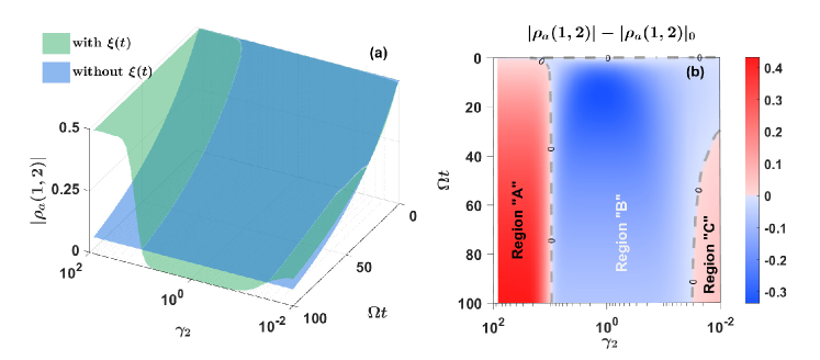
Figure 2: (a) Time evolution of the atomic coherence ($|\rho_{a}(1,2)|$, $\rho_{a}=\mbox{Tr}_{c}\{\rho_{ac}\}$) under different memory time $1/\gamma_{2}$ with noise and without noise of $\xi(t)$. The parameters are $\omega=\Omega=1$, $kx_{0}=0.08$, $\gamma_{1}=1$, and $\Gamma_{1}=\Gamma_{2}=1$. (b) Difference of the coherence between the cases with and without $\xi(t)$. $|\rho_{a}(1,2)|$ indicates the coherence with noise and $|\rho_{a}(1,2)|_{0}$ indicates the coherence without noise.

In this subsection, we will use numerical results to illustrate the mechanism proposed in Sec. III.1 and show how to use non-Markovian behaviors to protect coherence. We start from the noise $\xi(t)$ with a finite memory time $1/\gamma_{2}$. The time evolution of the atomic coherence with and without the noise $\xi(t)$ is plotted in Fig. 2 (a). The green surface indicates the coherence evolution in presence of the noise $\xi(t)$ with various $\gamma_{2}$, while the blue surface indicating the coherence evolution without noise. In order to show the effect of protection clearly, we also plot the difference of these two surfaces in Fig. 2 (b), where the red color indicates the noise $\xi(t)$ has a positive effect on coherence protection and the blue color indicates a negative effect. One can also check the purity $P={\rm Tr}(\rho_{a}^{2})$ (characterize the state is pure or not) follows the similar pattern at the early stage of the evolution (not shown). It is shown in Fig. 2 that the coherence protection highly depends on the memory time $1/\gamma_{2}$ of the noise $\xi(t)$. When $\gamma_{2}$ is above a threshold (region “A”), one can observe very strong protection of the atomic coherence. In contrast, below this threshold, the coherence loss is even faster (region “B”). However, at the right-bottom corner, there is a smaller region “C” with a small but positive effect of coherence protection.

Recall the mechanism proposed in Sec. III.1, since the coherence protection requires a fast varying speed of $G(t)$, the noise $\xi(t)$ should contain high-frequency components. The spectrum density in Eq. (21) shows that $g_{2}(\omega)$ has a finite high-frequency distribution only if $\gamma_{2}$ is large enough. Otherwise, when $\gamma_{2}\rightarrow 0$, $g_{2}(\omega)\propto\omega^{-2}$, the high-frequency components will quickly decrease to zero when $\omega$ is increasing. Physically, a Markovian noise $\xi(t)$ with $\gamma_{2}\rightarrow\infty$ has a uniform distribution on all the frequencies (white noise), corresponding to a $\delta(t,s)$ correlation function. Those high-frequency noises will be benefit to the coherence protection. Therefore, in Fig. 2, the Markovian noise ($\gamma_{2}\rightarrow\infty$) with more high-frequency components is more useful to the coherence protection, reflected by positive effect in region “A”. In contrast, in non-Markovian case, the frequency distribution of $\xi(t)$ is mainly concentrated in the low-frequency regime [see Eq. (21)]. The coupling $G(t)$ in Eq. (23) is not varying faster than $B(t)$, then $B(t)$ can not be treated as constant in the integral and its impact can not be eliminated. Even worse it may introduce extra loss of coherence as shown in the region “B” in Fig. 2 (b). However, we also notice there is another positive region “C” when $\gamma_{2}\rightarrow 0$, this is a different mechanism of averaging $\xi(t)$.

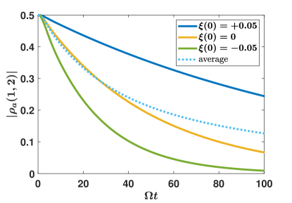
Figure 3: Coherence protection by super-long memory time of $\xi(t)$. The parameter is the same as Fig. 2.

When $\gamma_{2}\rightarrow 0$, the memory time of the noise $\xi(t)$ is even longer than the evolution time. During the evolution, $\xi(t)$ can be approximately treated as “not varying”, namely $\xi(t)=\xi(0)$. Therefore, for a particular trajectory, the time evolution is only determined by the initial value $\xi(0)$. For a particular realization, if $\xi(0)$ is randomly chosen as a positive number $\xi(0)=+c$, it will accelerate the dissipation. On the contrary, if $\xi(0)=-c$, it will decrease the dissipation. The average over the noise $\xi(t)$ is actually an average of these two effects. An example is shown in Fig. 3, where the dotted curve labeled with “average” is the average of the two curves $\xi(0)=+0.05$ and $\xi(0)=-0.05$. The curve $\xi(0)=0$ can be regarded as the case without noise $\xi(t)$. When adding the noise $\xi(t)$, the average effect lead to a higher residue coherence at $\Omega t=100$. At the early stage of the evolution (approximately $\Omega t<30$), the average causes a negative effect. This is in accordance with the results shown in Fig. 2, where the coherence protection has a negative effect at the early stage of the evolution at $\gamma_{2}\rightarrow 0$.

III.3 Combined effects of two noises

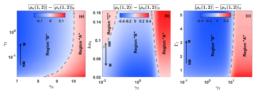
Figure 4: Coherence protection: impacts from two noises. The performance is characterized by the difference of average coherence of $\overline{|\rho_{a}(1,2)|}=\frac{1}{\Omega T}\int_{0}^{\Omega T=100}|\rho_{a}(1,2)|(t)dt$ [with $\xi(t)$] and $\overline{|\rho_{a}(1,2)|_{0}}$ [without $\xi(t)$]. With the change of the factors indicated by the $y$-axis of each sub-plot, the arrows show the direction of transition from non-Markovian (NM) to Markovian (M) regime for the quantized noise $z_{t}^{*}$. The parameters are $\omega_{0}=\Omega=1$, $\gamma_{1}=0.5$, $kx_{0}=0.08$, $G_{0}=1$, and $\Gamma_{1}=\Gamma_{2}=1$, unless specified explicitly in each sub-plot.

In the last subsection, we focus on the non-Markovian effect of $\xi(t)$ and analyze the mechanism of the coherence protection. Besides the noise $\xi(t)$, there is also another quantized noise $z_{t}^{*}$ from the bosonic bath $H_{\mathrm{B}}=\sum_{i}\omega_{i}b^{\dagger}b_{i}$. From the view of the atom, the cavity plus the bath is a hierarchical environment, whose effective correlation function is complicated Mazzola et al. (2009). Here, we only make a simple qualitative analysis. The non-Markovianity of the hierarchical environment is determined by several factors.

First, a longer memory time $1/\gamma_{1}$ certainly leads to a non-Markovian effect, although such an impact is indirectly transmitted to the atom through the cavity. In Fig. 4 (a), when $\gamma_{1}$ is small, the hierarchical environment is in the non-Markovian regime. Typically, high-frequency components is weak in non-Markovian noise, and Markovian noise contains more high-frequency components. Taking the O-U noise in Eq. (20) as an example, when $\gamma_{1}$ is small, the high-frequency part in the spectrum density is suppressed as shown in Eq. (21). As we have analyzed, the mechanism of coherence protection is the low-frequency noise can be controlled by another high-frequency noise. If a non-Markovian noise $z_{t}^{*}$ (long memory time) causes a slow evolution of the system, we only need to use a moderately high-frequency $\xi(t)$ to cancel the impact of $z_{t}^{*}$. It is reflected in Fig. 4 (a) as the threshold of $\gamma_{2}$ to achieve positive effect of protection is relatively low when $\gamma_{1}$ is small. On the contrary, when $\gamma_{1}$ is large, $z_{t}^{*}$ is a Morkov noise, containing more high-frequency components. Then, we need to use a much higher frequency noise to suppress it. Reflected in Fig. 4 (a), the threshold becomes larger when $\gamma_{1}$ is increased.

Second, the coupling strength $G$ is also crucial to the non-Markovianity of the noise $z_{t}^{*}$. One one hand, taking the cavity plus the bath as combined environment, a stronger coupling to the system certainly causes stronger non-Markovian feedback effect. On the other hand, the cavity (pseudo-environment) can be regarded as a tiny reservoir, the “water level” in the reservoir is determined by both the injection rate $G$ and the leakage rate $\Gamma_{1}$. For a fixed $\Gamma_{1}$, a smaller $G$ will cause all the “water” is drained. Certainly, there will be no feedback effect (backflow). In our case, although the coupling $G(t)$ is a stochastic function, the balanced position $x_{0}$ still indicates an average effect. Without the second noise $\xi(t)$, a larger $x_{0}$ ($kx_{0}<\pi/2$) means a stronger coupling, namely a stronger non-Markovian effect of $z_{t}^{*}$. Then, as we have analyzed above, a moderately Markovian (high-frequency) noise $\xi(t)$ can successfully suppress $z_{t}^{*}$. On the contrary, a small $x_{0}$ corresponds to a Markovian evolution. Thus, one need a noise $\xi(t)$ with a higher frequency (more Markovian) with a larger $\gamma_{2}$. This is illustrated by the numerical result in Fig. 4 (b). When $kx_{0}$ is decreased (noise $z_{t}^{*}$ is changing from non-Markovian to Markovian), the threshold to achieve positive effect of coherence protection is increased. As for the anomalous region “C”, the reason for a positive effect is the same as we have discussed in Fig. 3.

Third, the dissipation rate to the bath $\Gamma_{1}$ can also determine the non-Markovianity of $z_{t}^{*}$. When the cavity is treated as the “reservoir”, the a small dissipation rate leads to a strong backflow to the system. In the limiting case, if $\Gamma_{1}\rightarrow 0$, the total environment becomes a single cavity with a single mode. This is definitely a very strong non-Markovian environment. Therefore, it is shown in Fig. 4 (c) that with the increase of $\Gamma_{1}$, the threshold of achieving positive effect is also increased.

In a brief summary, we use the numerical results to illustrate that a low-frequency noise can be suppressed by a high-frequency noise. This provides a clue to engineer the environment Liu et al. (2011) so that making the combined decoherence effect of two noises is reduced. The question (ii) raised in Sec. I is partially answered from the perspective of non-Markovian properties of the noises.

III.4 Non-Markovian noise $\eta(t)$

As we have mentioned in Sec. I, in the topic of coherence protection by noise, one important question is how to add the second noise to make the effect of protection is positive. Besides the noise $\xi(t)$ in coupling, another noise is often appear as the dephasing noise for the atom. Particularly, in the cases discussed Appendix A, the noise the external field often caused a fluctuation in the energy gap of the qubit, represented by $\eta(t)$ in Eq. (6). In this subsection, we will mainly focus on this type of noise.

In order to compare with the case of $\xi(t)$, we rotate the Hamiltonian with respect to $S=\frac{\Phi(t)}{2}\sigma_{z}$, where $\Phi(t)=\int_{0}^{t}\eta(s)ds$. The Hamiltonian in this rotating frame becomes

$$H_{{\rm JC}}^{\prime} =e^{iS}H_{{\rm JC}}e^{-iS}-\frac{\partial S}{\partial t}$$

$$=\frac{\omega_{0}}{2}\sigma_{z}+\Omega a^{\dagger}a+G_{0}e^{i\Phi(t)}a\sigma_{+}+G_{0}e^{-i\Phi(t)}a^{\dagger}\sigma_{-}.$$ (28)

The original noise in $\omega(t)=\omega_{0}+\eta(t)$ has been transformed into a phase noise $\Phi(t)$ in the coupling. Moreover, different from the stochastic coupling $G(t)=G_{0}\sin\left\{k\left[x_{0}+\xi(t)\right]\right\}$, the stochastic coupling $G_{0}e^{i\Phi(t)}$ has a fixed amplitude, but a random phase factor. This will cause slightly difference on the coherence protection as shown below.

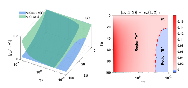
Figure 5: Time evolution of the atomic coherence ($|\rho_{a}(1,2)|$) under different memory time $1/\gamma_{3}$ with and without noise of $\eta(t)$. The parameters are $\omega_{0}=\Omega=1$, $G_{0}=0.1$, $\gamma_{1}=1$, and $\Gamma_{1}=\Gamma_{2}=1$. (b) Difference of the coherence between the cases with and without $\eta(t)$. $|\rho_{a}(1,2)|_{0}$ indicates the coherence without noise.

In Fig. 5, we investigate the impact of the memory time $\eta(t)$. Similar to the case of $\xi(t)$, the coherence protection has a positive effect in the Markovian regime. According to the mechanism of coherence protection discussed in Sec. III.1, a high-frequency noise is more welcome, so that region “A” is positive. However, different from the special region “C” in Fig. 2 (b), the positive region at $\gamma_{3}\rightarrow 0$ does not appear in Fig. 5. This is because the average mechanism shown in Fig. 3 is not applicable to the Hamiltonian (28). The noise $\xi(t)$ causes a fluctuation around the balanced value $G_{0}\sin(kx_{0})$, so the amplitude of $G$ is fluctuating. As comparison, the noise $\eta(t)$ only changes the phase of the coupling $G$ without changing its amplitude. Mathematically, $\gamma_{3}\rightarrow 0$ leads to $G(t)\rightarrow G_{0}e^{\pm i\phi_{c}}$ ($\phi_{c}$ is a constant phase factor due to super-long memory time) in Eq. (23-25). Then, it is straightforward to check that adding a constant phase factor only results in a phase factor $e^{\pm i\phi_{c}}$ on the solution $A(t)$ as $A(t)\rightarrow A(t)e^{\pm i\phi_{c}}$. This has no contribution to the coherence in Eq. (26). Therefore, in the limit of $\gamma_{3}\rightarrow 0$, we see $|\rho_{a}(1,2)|$ is asymptotically approaching $|\rho_{a}(1,2)|_{0}$. The positive region like region “C” in Fig. 2 (b) at $\gamma_{3}\rightarrow 0$ does not appear in Fig. 5.

From this example, we see the form of the second noise is also crucial to the coherence protection. We would like to emphasize that all the results shown in this section only imply that the quantized noise $z_{t}^{*}$ can be suppressed by $\eta(t)$ or $\xi(t)$. It is also possible to show the opposite case that by comparing the coherence with and without $z_{t}^{*}$, the impacts of a classical noise can be weaken, too. Certainly, the condition to achieve that goal must be different (maybe the coupling form is different from $\eta(t),$or the required spectrum density is different). Certainly, all of these topics are valuable in another study elsewhere.

III.5 Outlook: Alternative perspective of coherence protection

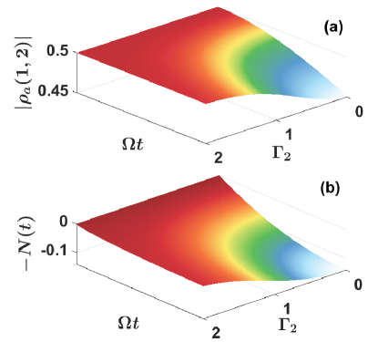
Figure 6: Time evolution of the atomic coherence $|\rho_{a}(1,2)|$ vs. the atom-cavity entanglement $N(t)$ Vidal and Werner (2002); Vidal (2000). To compare with the coherence, a minus sign is added artificially as [$-N(t)$], lower values represent stronger entanglement. The parameters for all the sub-plots are $\omega=\Omega=1$, $\Gamma_{1}=0.5$, $\gamma_{1}=1$, and $x_{0}=0.1$.

In the previous subsections, we have made an extensive investigation on coherence protection by noise. At last, we would like to analyze the coherence protection in a different perspective and it is our hope that it may shed new light on answering the question (i) raised in Sec. I.

Besides the mathematical picture, we would also analyze the coherence protection from a physical perspective. Physically, there are mainly three reasons causing the loss of coherence in our model, (1) atom-cavity entanglement, (2) atom-bath entanglement, and (3) energy dissipation to the bath. These three processes happen at the same time in the evolution and the coherence loss is a combined effect. First, the decay rate to the bath $H_{{\rm B}}$ is proportional to the photon number $|B(t)|^{2}$ as

$$\frac{d}{dt}|D_{k}(t)|^{2}=-|g_{k}|^{2}|B(t)|^{2}.$$ (29)

In order to reduce the decay rate to the bath, one need to suppress the photon number $|B(t)|^{2}$ in the cavity. However, in this particular model, reducing the photon number $|B|^{2}$ happens to also reduce the entanglement between the atom and the cavity, since the atom-cavity entanglement can be measured by the concurrence Wootters (1998) as

$$C(\rho_{ac})=4|A|^{2}|B|^{2}.$$ (30)

In Eq. (24), the changing of $B(t)$ at the early stage of the evolution mainly comes from the contribution of $-iG(t)A(t)$, because $I(t)$ is a slow varying term. We have already shown that the average of a noisy $G(t)$ is close to zero in the time integral. Therefore, a slow increasing of the photon number $|B(t)|^{2}$ at the early stage of the evolution can prevent not only the decay to the bath but also the entanglement generation.

In this particular model, the atom-cavity entanglement generation is directly related the coherence protection [see Eq. (26) and Eq. (30)]. In Fig. 6, we numerically show the connection between coherence protection and the atom-cavity entanglement generation. Roughly, the patterns of the dynamics are almost identical. For more details of the numerical simulation, see Appendix D.

In a more general picture shown in Fig. 1, the cavity here can be regarded as part of hierarchical environment. It is known that a quantum system will lose its coherence when taking the trace of the environmental degrees of freedom, if the quantum system is entangled with the environment. For this particular example, we see that using a noise to destroy the entanglement generation can protect the coherence. In a more general case with a hierarchical environment, this might be a clue to find what types of the second noise has a positive effect on coherence protection and partially answer the question (i) raised in Sec. I.

Interestingly, From the perspective of destroying the atom-cavity entanglement, the anomalous pattern in Fig. 2 can be also explained by non-Markovian effect on entanglement generation. Markovian noise corresponding to a larger $\gamma_{2}$ is more powerful to destroy the atom-cavity entanglement generation thus the coherence is protected (region “A”). In contrast, non-Markovian noise corresponding to a smaller $\gamma_{2}$ is often considered to be good to the entanglement generation Ding et al. (2021); Zhao (2019); Zhao et al. (2011, 2012); Shen et al. (2017, 2018a, 2018b, 2018c), so that the coherence is destroyed (region “B”). The interesting phenomenon arises in region “C” in Fig. 2 (b) can be also explained by the entanglement generation in non-Markovian dynamics, which has been widely studied in several references Zhao et al. (2011, 2012); Zhao (2019); Zhao et al. (2017). For example, recall the results in Refs. Zhao et al. (2011); Zhao (2019), the entanglement generated in a non-Markovian environment characterized by O-U correlation function reaches the maximum value when the memory time is neither too big nor too small. Therefore, the minimum coherence should appear when $\gamma_{2}$ is neither too big nor too small. Reflected in Fig. 2 (b), there is a “negative effect” window opened between two “positive effect” regions.

Certainly, all the analysis above is only based on a very special case, and the connection between entanglement generation and coherence protection is far more complicated than we discussed here. But, we would like to emphasize that a future research on this topic may open a new path to design more coherence protection schemes by using noise.

IV Discussion and Conclusion

In this paper, we show how to protect the quantum coherence by using noise. As an example, we solve the J-C model coupled to an external environment and derive the master equation incorporating the non-Markovian behaviors from both the classical noise and the quantized bath. The master equation itself is valuable in theoretical study on the joint non-Markovian effect of two noises. It may also become a powerful tool to investigate the indirectly interaction of the two noises in future researches. Beyond the theoretical significance, we also show that the atomic coherence can be protected by adding another noise. By analyzing the non-Markovian properties of the two noises, we draw a conclusion that the decoherence caused by a low-frequency noise can be eliminated by another noise containing higher-frequency components. The results show that the non-Markovian properties (particularly the memory time) of the two noises are crucial to the performance of the coherence protection. At last, as an outlook, we also discuss the relation between the atom-cavity entanglement and the atomic coherence.

This work may provide a deeper understanding of noise. In most cases, noise is often supposed to be harmful to quantum coherence. However, the example discussed in this paper illustrates that noise can be helpful to maintain quantum coherence in certain cases. Similar to several other studies Yi et al. (2003); Jing and Wu (2013); Jing et al. (2014, 2018); Khodorkovsky et al. (2008); Chen et al. (2017a), the results presented in this paper provide an example once again that noise can lead not only troubles but also benefits. This may shed more light on the understanding of noise. Besides, it is very interesting that the trouble caused by one noise ($z_{t}^{*}$) happens to be eliminated by another noise ($\eta$ or $\xi$). Similar results have been observed in several other theoretical studies of different models Jing and Wu (2013); Jing et al. (2018); Qiao et al. (2019). Here, we analyze the reason for the coherence protection from two aspects. Mathematically, a slow-varying function can be eliminating in the time integral by a fast varying function. Physically, the relation between entangling to the environment and the loss of coherence inspire us to search a possible way to protect coherence by preventing it to be entangled with the environment. This may open a new path to design new coherence protection schemes by using noise.

Appendix A Alternative examples of hierarchical environment

In Fig. 1, we discuss a scenario that quantum system is indirectly coupled to the bath through “pseudo-environment” illustrated by J-C model coupled to an external bath. Besides the example in cavity-QED system discussed in the main text, we also present an alternative realization in circuit-QED system You and Nori (2005, 2011). As shown in Fig. 7 (a), one of the resonator can be defined as the quibt when the gap between the ground state and the excited state is huge. Then, the other resonator can be modeled as a harmonic oscillator. The tunable (time-dependent) coupling is realized by the external flux $\phi_{x}(t)$, which is discussed in Ref. Tian et al. (2008). Finally, the model can be described by the Hamiltonian in Eq. (2), and some other tunable coupling schemes such like flux qubit coupled to a resonator are also discussed in Refs. van den Brink et al. (2005); Averin and Bruder (2003); Plourde et al. (2004); Hime et al. (2006).

Besides the cavity-QED system and the circuit-QED system, a huge category of physical models of hierarchical environment is often studied in the semiconductor quantum dot system. In quantum dots, the spin degree of freedom is rarely coupled to external noises resulting in their super-long coherence time Burkard et al. (2020). Particularly, with the help of isotopic purification that suppresses magnetic noise from surrounding nuclear spins, the coherence time of spin qubit can exceed one second Tyryshkin et al. (2012), making it to be hopeful candidate of the quantum processor. However, through the spin-orbit interaction, spin states can indirectly coupled to noisy environments, which causes spin relaxation/dephasing Zhao et al. (2016); Zhao and Hu (2018). Here, we analyze a double quantum dot model which is used to realize spin-photon interface Mi et al. (2018), where a single electron tunneling in double quantum dots, forming two charge (orbital) states $|L\rangle$ and $|R\rangle$. The applied magnetic field $B_{0}$ along $z$-direction produces two spin states $|\uparrow\rangle$ and $|\downarrow\rangle$. A nano-magnet produces a field gradient $B_{x}$ in $x$-direction, making the magnetic field in left dot and right are different. The schematic diagram is plotted in Fig. 7 (b). In the basis $\{|L,\uparrow\rangle,|L,\downarrow\rangle,|R,\uparrow\rangle,|R,\downarrow\rangle\}$, the Hamiltonian can be written as

$$H_{DQD}=\epsilon_{0}\tau_{z}+t_{C}\tau_{x}+B_{0}\sigma_{z}+B_{x}\sigma_{x}\tau_{x},$$ (31)

where $\tau_{i}$ and $\sigma_{i}$ are the Pauli matrices in orbital space and spin space respectively, $\epsilon_{0}$ is the detuning between left and right dot and $t_{C}$ is the tunneling barrier.

In this example the charge (orbital) degrees of freedom plays the role of “pseudo-environment” $H_{E}$ shown in Fig. 1, connecting electron spin to the “bath” such as charge fluctuation or phonon noise. Practically, a fluctuation in magnetic field $B_{0}\rightarrow B_{0}+\delta B(t)$ causing a dephasing, similar to the case discussed in Eq. (6). Alternatively, a charge noise in the detuning $\epsilon_{0}\rightarrow\epsilon_{0}+\delta\epsilon(t)$ can drive the electron continuously jumping between two dots thus suffering different $x$-direction magnetic field. This is quite similar to the example we discussed in Sec. III, which is a time-dependent interaction between the system and the pseudo-environment.

Some other examples can be also found in recent the experimental progress Burkard et al. (2020). For example, when the semiconductor quantum dots are coupled to a cavity, the system can be just roughly described by a simplified J-C model Burkard et al. (2020). The mathematical description of the dynamics of the system would be quite similar to the results presented in this paper.

Anyway, in semiconductor quantum dots, the electron spin is typically indirectly coupled to the environment through spin-orbit interaction, which naturally provides a huge category of examples of hierarchical environment. It is worth to note that in quantum dot systems, the charge noise mainly plays the role of the classical noise. For example, the fluctuation of the magnetic field often causes the dephasing of the qubit. In this case, the classical noise is in the form of $\eta(t)$ as shown in Eq. (6).

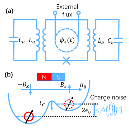
Figure 7: Alternative examples of hierarchical environment. (a) Another possible realization of J-C model Eq.  in circuit-QED systems You and Nori (2005, 2011). Two micro-resonators are coupled by a radio frequency SQUID coupler Tian et al. (2008). (b) Single electron in double quantum dot. A nano-magnet produces the gradient of the magnetic field to enhance the spin-orbit interaction.

Appendix B Derivation of master equation

B.1 noise in $\eta(t)$

In this section, we show how to derive the master equation from the NMQSD equation (11). Taking the $\eta(t)$ noise as an example and assuming the coupling $G(t)=G_{0}\sin(kx_{0})$ is a constant, the time derivative of the density matrix can be written as

$$\frac{d}{dt}\rho_{ac} = \frac{d}{dt}\left\langle M\left\{|\psi_{t}\rangle\langle\psi_{t}|\right\}\right\rangle,$$ (32)

$$= \left\langle M\left\{\frac{d}{dt}|\psi_{t}\rangle\langle\psi_{t}|+|\psi_{t}\rangle\frac{d}{dt}\langle\psi_{t}|\right\}\right\rangle,$$

$$= \langle M\{[-iH_{{\rm 0}}-i\frac{\eta(t)}{2}\sigma_{z}+az_{t}^{\ast}-a^{\dagger}\bar{O}]|\psi_{t}\rangle\langle\psi_{t}|$$

$$+ |\psi_{t}\rangle\langle\psi_{t}|[iH_{{\rm 0}}+i\frac{\eta(t)}{2}\sigma_{z}+a^{\dagger}z_{t}-\bar{O}^{\dagger}a]\}\rangle,$$

where $H_{0}=\frac{\omega_{0}}{2}\sigma_{z}+\Omega a^{\dagger}a+G_{0}\sin(kx_{0})(a\sigma_{+}+a^{\dagger}\sigma_{-})$, and the time derivative of the stochastic state vector $\frac{d}{dt}|\psi_{t}\rangle$ is substituted by the NMQSD Eq. (11). Noticing that the statistical mean $M_{1}\{\cdot\}$ and $\langle\cdot\rangle$ are averaging over noises, if the kernel functions are independent of noise variables, the mean values will be the kernel functions themselves.

In order to compute the right-hand-side of Eq. (32), we introduce two lemmas and prove them by using the Novikov theorem and the chain rule of the functional derivative.

Lemma 1.1

$$\left\langle M\left\{-i\eta(t)|\psi_{t}\rangle\langle\psi_{t}|\right\}\right\rangle$$

$$=\left\langle M\left\{|\psi_{t}\rangle\langle\psi_{t}|\bar{D}^{\dagger}-\bar{D}|\psi_{t}\rangle\langle\psi_{t}|\right\}\right\rangle,$$ (33)

where $\bar{D}=i\int_{0}^{t}ds\left\langle\eta(t)\eta(s)\right\rangle D(t,s,\eta)=i\int_{0}^{t}ds\alpha_{3}(t,s)\frac{\delta}{\delta\xi(s)}$ is a functional derivative operator.

Proof: According to the chain rule for functional derivative the term $\left\langle M\left\{-i\eta(t)|\psi_{t}\rangle\langle\psi_{t}|\right\}\right\rangle$ can be expanded as

$$\left\langle M\left\{-i\eta(t)|\psi_{t}\rangle\langle\psi_{t}|\right\}\right\rangle=-iM\left\{\left\langle\eta(t)|\psi_{t}\rangle\langle\psi_{t}|\right\rangle\right\},$$

$$=-iM\left\{\int_{0}^{t}ds\left\langle\eta(t)\eta(s)\right\rangle\left\langle\frac{\delta(|\psi_{t}\rangle\langle\psi_{t}|)}{\delta\eta(s)}\right\rangle\right\},$$

$$=-iM\left\{\int_{0}^{t}ds\left\langle\eta(t)\eta(s)\right\rangle\left\langle\frac{\delta|\psi_{t}\rangle}{\delta\eta(s)}\langle\psi_{t}|+|\psi_{t}\rangle\frac{\delta\langle\psi_{t}|}{\delta\eta(s)}\right\rangle\right\},$$

$$=\left\langle M\left\{|\psi_{t}\rangle\langle\psi_{t}|\bar{D}^{\dagger}-\bar{D}|\psi_{t}\rangle\langle\psi_{t}|\right\}\right\rangle,$$ (34)

where the functional derivative $\frac{\delta}{\delta\eta(s)}$ is replaced by a time-dependent (maybe also noise dependent) operator $D(t,s,\eta)$ defined as

$$\frac{\delta}{\delta\eta(s)}|\psi_{t}\rangle=D(t,s,\eta)|\psi_{t}\rangle.$$ (35)

Since the stochastic state vector can be obtained by a stochastic evolution operator acting on the initial state $|\psi_{t}\rangle=U(t,\eta)|\psi_{0}\rangle$, then the existence of such an operator $D$ can be proved as

$$\frac{\delta}{\delta\eta(s)}|\psi_{t}\rangle =\left[\frac{\delta}{\delta\eta(s)}U(t,\eta)\right]|\psi(0)\rangle,$$

$$=\left[\frac{\delta}{\delta\eta(s)}U(t,\eta)\right]U^{-1}(t,\eta)|\psi_{t}\rangle.$$ (36)

As a result, the operator $D$ can be formally defined as $D(t,s,\eta)=\left[\frac{\delta}{\delta\eta(s)}U(t,\eta)\right]U^{-1}(t,\eta)$. According to Eq. (35) and noticing that the order of the averaging operation $M_{1}\{\cdot\}$ and $\langle\cdot\rangle$ can be swapped, lemma 1.1 is proved.

Lemma 1.2

$$\left\langle M_{1}\left\{z_{t}^{*}|\psi_{t}\rangle\langle\psi_{t}|\right\}\right\rangle=\left\langle M_{1}\left\{\bar{O}|\psi_{t}\rangle\langle\psi_{t}|\right\}\right\rangle.$$ (37)

The proof of this lemma for the quantized noise is different from classical noise. It can be also found in Refs. Yu et al. (1999).

With lemma 1.1 and 1.2, one can substitute the results into Eq. (32) to obtain a master equation as

$$\frac{d}{dt}\rho=-i\left[H_{0},\rho\right]$$

$$+\left[a,\left\langle M\left\{|\psi_{t}\rangle\langle\psi_{t}|\bar{O}^{\dagger}\right\}\right\rangle\right]+\left[\left\langle M\left\{\bar{O}|\psi_{t}\rangle\langle\psi_{t}|\right\}\right\rangle,a^{\dagger}\right]$$

$$+\left[\sigma_{z},\left\langle M\left\{|\psi_{t}\rangle\langle\psi_{t}|\bar{D}^{\dagger}\right\}\right\rangle\right]+\left[\left\langle M\left\{\bar{D}|\psi_{t}\rangle\langle\psi_{t}|\right\}\right\rangle,\sigma_{z}\right].$$ (38)

The operator $\bar{D}$ can be determined by the consistency condition $\frac{\delta}{\delta\eta(s)}\frac{d}{dt}|\psi_{t}\rangle=\frac{d}{dt}\frac{\delta}{\delta\eta(s)}|\psi_{t}\rangle$. The left-hand-side can be written as

$$\frac{\delta}{\delta\eta(s)}\frac{d}{dt}|\psi_{t}\rangle =\frac{\delta}{\delta\eta(s)}\left(H_{{\rm eff}}|\psi_{t}\rangle\right)$$

$$=\frac{\delta}{\delta\eta(s)}H_{{\rm eff}}|\psi_{t}\rangle+H_{{\rm eff}}\frac{\delta}{\delta\eta(s)}|\psi_{t}\rangle$$

$$=\frac{\delta}{\delta\eta(s)}H_{{\rm eff}}|\psi_{t}\rangle+H_{{\rm eff}}D|\psi_{t}\rangle,$$ (39)

while the right-hand-side can be written as

$$\frac{d}{dt}\frac{\delta}{\delta\eta(s)}|\psi_{t}\rangle =\frac{d}{dt}\left[D(t,s,\eta)|\psi_{t}\rangle\right]$$

$$=\frac{d}{dt}D|\psi_{t}\rangle+D\frac{d}{dt}|\psi_{t}\rangle$$

$$=\frac{d}{dt}D|\psi_{t}\rangle+DH_{{\rm eff}}|\psi_{t}\rangle.$$ (40)

Equating left-hand-side and right-hand-side, one can obtain

$$\frac{d}{dt}D=\left[H_{{\rm eff}},D\right]+\frac{\delta}{\delta\eta(s)}H_{{\rm eff}}.$$ (41)

Integrating over an infinitesimal time interval $s_{-}<t<s_{+}$ around $t=s$,

$$D(t=s_{+},s,\eta)-D(t=s_{+},s,\eta)$$

$$=\int_{s_{-}}^{s_{+}}dt\left\{-i\frac{1}{2}\delta(t,s)\sigma_{z}+\left[H_{{\rm eff}},D\right]\right\},$$ (42)

since the functional derivative $\frac{\delta}{\delta\eta(s)}$ is only non-zero on the term $\frac{\eta(t)}{2}\sigma_{z}$ in $H_{{\rm eff}}$. In the integral, the contribution from the second term is zero since $\left[H_{{\rm eff}},D\right]$ is finite and the integration interval is close to zero, $s_{+}-s_{-}\rightarrow 0$. Therefore, at the boundary $s=t$, the boundary condition reads $D(t=s,s,\eta)=-i\frac{1}{2}\sigma_{z}$.

Similarly, one can also use the consistency condition $\frac{\delta}{\delta z_{t}^{*}}\frac{d}{dt}|\psi_{t}\rangle=\frac{d}{dt}\frac{\delta}{\delta z_{t}^{*}}|\psi_{t}\rangle$ to obtain

$$\frac{d}{dt}O=\left[H_{{\rm eff}},D\right]+a^{\dagger}\frac{\delta}{\delta z_{s}^{*}}\bar{O},$$ (43)

with the boundary condition $O(t=s,s,z^{*})=a$.

In most cases, we can approximately assume the operators $D$ and $O$ are all noise-independent Xu et al. (2014). Then, the master equation can be further simplified as

$$\frac{d}{dt}\rho=-i\left[H_{{\rm 0}},\rho\right]+\left\{\left[a,\rho\bar{O}^{\dagger}\right]+\left[\sigma_{z},\rho\bar{D}^{\dagger}\right]+{\rm h.c.}\right\},$$ (44)

Here, the master equation does not formally contain a cross-term combining the impact from both $z_{t}^{*}$ and $\eta(t)$, this is because the two noises are independent (not correlated noise). More details on the discussion of correlated noise can be found in Corn and Yu (2009); Jing et al. (2015). However, if we compute the exact solution of operators $D$ and $O$, one may find that $O$ has an impact on $D$ and $D$ also has an impact on $O$. Therefore, interference effect between two noises may exist. One example can be found in Ref. Zhao et al. (2017).

B.2 noise in $\xi(t)$

In the above subsection, we have shown the detailed derivation of the master equation in the presence of $\eta(t)$ noise, now, we will briefly show the case of $\xi(t)$ noise discuss the difference between them. When, $\eta(t)=0$ and $\xi(t)\neq 0$, the time derivative of $|\psi_{t}\rangle$ is

$$\frac{d}{dt}\rho = \langle M\{[-iH_{{\rm 0}}^{\prime}-i\frac{G(t)}{2}V+az_{t}^{\ast}-a^{\dagger}\bar{O}]|\psi_{t}\rangle\langle\psi_{t}|$$ (45)

$$+ |\psi_{t}\rangle\langle\psi_{t}|[iH_{{\rm 0}}^{\prime}+i\frac{G(t)}{2}V+a^{\dagger}z_{t}-\bar{O}^{\dagger}a]\}\rangle,$$

where $H_{0}^{\prime}=\frac{\omega_{0}}{2}\sigma_{z}+\Omega a^{\dagger}a$, $V=a\sigma_{+}+a^{\dagger}\sigma_{-}$. Now, the noise is included in the coupling $G(t)$. Similar to Eq. (33), one can prove

$$\left\langle M\left\{-iG(t)|\psi_{t}\rangle\langle\psi_{t}|\right\}\right\rangle$$

$$=\left\langle M\left\{|\psi_{t}\rangle\langle\psi_{t}|\bar{D}_{G}^{\dagger}-\bar{D}_{G}|\psi_{t}\rangle\langle\psi_{t}|\right\}\right\rangle,$$ (46)

where $\bar{D}=i\int_{0}^{t}ds\left\langle G(t)G(s)\right\rangle D_{G}(t,s,G)=i\int_{0}^{t}ds\left\langle G(t)G(s)\right\rangle\frac{\delta}{\delta G(s)}$ is a functional derivative operator with the boundary condition $D_{G}(t,s=t,G)=V$. Because we take the functional derivative with respect to $G(t)$ here, the correlation is in the form of $\left\langle G(t)G(s)\right\rangle$. However, if $\langle\xi(t)\xi(s)\rangle=\alpha_{2}(t,s)$ is known, it is straightforward to compute $\left\langle G(t)G(s)\right\rangle$. Eventually, the master equation can be written as

$$\frac{d}{dt}\rho=-i\left[H_{{\rm 0}}^{\prime},\rho\right]+\left\{\left[a,\rho\bar{O}^{\dagger}\right]+\left[V,\rho\bar{D}_{G}^{\dagger}\right]+{\rm h.c.}\right\}.$$ (47)

B.3 Equation for operator $O$

According to the consistency condition (43), we find the solution of $O$ operator in Eq. (19) is

$$O(t,s,z^{*})=\sum_{i=1}^{4}f_{i}(t,s)O_{i}+\int_{0}^{t}f_{5}(t,s,s^{\prime})z_{s^{\prime}}^{*}ds^{\prime}O_{5},$$ (48)

with the basis operators $O_{1}=a$, $O_{2}=\sigma_{-}aa^{\dagger}$, $O_{3}=\sigma_{-}a^{\dagger}a$, $O_{4}=\sigma_{z}a$, and $O_{5}=\sigma_{-}a$. The coefficients satisfy the following equations

$$\partial_{t}f_{1}(t,s) = i\Omega f_{1}+i\frac{G}{2}f_{2}-i\frac{G}{2}f_{3}-f_{1}F_{1}-f_{4}F_{4},$$ (49)

$$\partial_{t}f_{2}(t,s) = i\omega f_{2}+iGf_{1}-iGf_{4}-f_{1}F_{2}+f_{4}F_{2},$$ (50)

$$\partial_{t}f_{3}(t,s) = i\omega f_{3}-iGf_{1}-iGf_{4}+f_{1}F_{2}+f_{4}F_{2}-2f_{3}F_{4}-F_{5}^{\prime}(t,s),$$ (51)

$$\partial_{t}f_{4}(t,s) = i\Omega f_{4}-i\frac{G}{2}f_{2}-i\frac{G}{2}f_{3}-f_{4}F_{1}-f_{1}F_{4},$$ (52)

$$\partial_{t}f_{5}(t,s,s^{\prime}) = i\omega f_{5}+i\Omega f_{5}-f_{5}F_{1}-f_{5}F_{4}-f_{1}F_{5}^{\prime}+f_{4}F_{5}^{\prime},$$ (53)

where $F_{i}(t)=\int_{0}^{t}\alpha(t,s)f_{i}(t,s)ds$ ($i=1,2,3,4$) and $F_{5}^{\prime}(t,s^{\prime})=\int_{0}^{t}\alpha(t,s)f_{5}(t,s,s^{\prime})ds$, and the initial conditions are

$$f_{1}(t,t)=1,\quad f_{i}(t,t)=0,\quad(i=2,3,4)$$ (54)

$$f_{5}(t,t,s^{\prime})=0,\quad f_{5}(t,s,t)=f_{3}-f_{2}.$$ (55)

As we have discussed in Sec. II, both Eqs. (18) and (14) are reduced to Markovian form when $\alpha_{1}(t,s)=\Gamma_{1}\delta(t,s)$ leading to a simplified $\bar{O}$ with only the $O_{1}$ term, because $F_{1}(t)=\int_{0}^{t}\Gamma_{1}\delta(t,s)f_{1}(t,s)ds=\frac{\Gamma_{1}}{2}$ and all the other coefficients $F_{i}=0$ ($i=2,3,4,5$), where $F_{5}=\int_{0}^{t}\alpha(t,s)F_{5}^{\prime}(t,s)ds$. Therefore, the other terms can be regarded as the non-Markovian corrections to the $O_{1}$ term. Typically these correction terms are quite small, particularly the noise-dependent term $O_{5}$ is much smaller than the other terms (Detailed study about the impact of noise-dependent term can be found in Ref. Xu et al. (2014) with a two-qubit dissipative model. Here we simply use numerical simulation to show $\frac{|F_{5}|}{|F_{1}|}\approx 10^{-4}$ in Fig. 8. Thus, it is safe to neglect the $O_{5}$ term and Eq. (48) is reduced to

$$O(t,s)=\sum_{i=1}^{4}f_{i}(t,s)O_{i},$$ (56)

where $O(t,s)$ becomes independent of $z_{t}^{*}$. Besides, it is more important to note that the memory time used to generate Fig. 8 is $\gamma_{1}=0.5$, corresponding to a relative non-Markovian value. When we have a shorter memory time $1/\gamma_{1}$ ($\gamma_{1}$ is larger), the correlation function will even close to a delta-function. Then, the delta-like correlation function leads to $F_{5}\rightarrow 0$ as we have discussed. In that case, it is even more reasonable to neglect $F_{5}$ in Eq. (56).

In the most general case, there is a systematic way to expand $O$ operator up to certain orders Yu et al. (1999); Li et al. (2014). With a noise dependent $O$ operator, the master equation (38) can be also simplified to a Lindblad form by following the procedure developed in Ref. Chen et al. (2014). In the derivation of the master equation, we also assume the temperature of the bath is zero. The master equation of the finite temperature case can be obtained by using the technique in Ref. Yu (2004). Several examples can be found in Refs. Zhao et al. (2009, 2017); Zhao (2019); Shi et al. (2013).

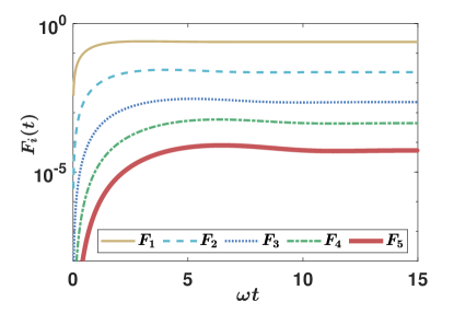
Figure 8: Time evolution of the coefficients in operator $\bar{O}$. The parameters are $\omega_{0}=\Omega=1,\Gamma_{1}=1$, and $\gamma_{1}=0.5$.

Appendix C Arbitrary correlation function

In the main text, we choose the O-U correlation function in Eq. (20), which, by definition, should be the correlation in Eq. (7) $\alpha_{1}(t,s)=\sum_{i}|g_{i}|^{2}e^{-i\omega_{i}(t-s)}$. We would like to emphasize that the NMQSD equation as well as the master equations we derived do not depend on the choice of correlation functions. The dynamical equations are applicable to all types of correlation functions. The choice of O-U correlation function is based on the need of showing transition from Markovian to non-Markovian regime and the impact of the memory time of the bath. Here, we show an example that the widely used $1/f$ noise can be obtained by summation of Lorentzian spectrum density in Eq. (21). Consider a set of Lorentzian spectrum density with different memory time $\gamma_{1}$ and statistical weight $W(\gamma_{1})=\frac{1}{\gamma_{1}^{2}}d\gamma_{1}$, then the summation of these Lorentzian spectrum leads to

$$\tilde{g}(\omega) = \int_{\gamma_{1L}}^{\gamma_{1H}}\frac{1}{\gamma_{1}^{2}}g(\omega)d\gamma_{1}$$ (57)

$$= \frac{\Gamma_{1}}{2\pi}\frac{1}{\omega}\arctan\left(\frac{\gamma_{1}}{\omega}\right)|_{\gamma_{1L}/\omega}^{\gamma_{1H}/\omega}\approx\frac{\Gamma_{1}}{4}\frac{1}{\omega},$$

which is proportional to $1/\omega$, thus called $1/f$ noise. The cut-off frequencies are labeled as $\gamma_{1H}$ and $\gamma_{1L}$.

In the numerical simulation, a noise $z(t)$ satisfying an arbitrary correlation function $M[z(t)z(s)^{*}]=\alpha(t-s)$ can be generated by two independent real Gaussian noises $z_{1}(t)$ and $z_{2}(t)$ satisfying $M[z_{1}(t)]=M[z_{2}(t)]=0$, and $M[z_{1}(t)z_{1}(s)]=M[z_{2}(t)z_{2}(s)]=\delta(t-s)$. One can first transform the correlation function into frequency domain as $|G(\omega)|^{2}=\int_{-\infty}^{\infty}\frac{1}{2\pi}\alpha(\tau)e^{-i\omega\tau}d\tau$, then taking the inverse Fourier transformation of the square root $G(\omega)=\sqrt{|G(\omega)|^{2}}$ as $R(t)=\int_{-\infty}^{\infty}\frac{1}{2\pi}G(\omega)e^{i\omega t}d\omega$. Finally the noise $z(t)$ can be constructed by

$$z(t)=\int_{-\infty}^{\infty}dsR(s)\frac{z_{1}(t-s)+iz_{2}(t-s)}{\sqrt{2}}.$$ (58)

Here, we also provide an example of applying other types of noises. According to Ref. Cheng et al. (2008), the so-called telegraph noise is generated as follows. The total evolution time period is separated into $N$ small intervals $\{t_{0},t_{1},t_{2}\ldots t_{N}\}$, in each interval $(t_{i}<t<t_{i+1})$, $x(t)=\pm 1$, as shown in Fig. 9 (inset-plot). At time $t_{i}$ the variable $\xi(t)$ may change its sign as $\xi(t_{i})=-\xi(t_{i-1})$ with probability $p$, and according to the normalization, the possibility that $\xi(t)$ keeps its value unchanged is $(1-p)$. Fig. 9 shows how does the jumping probability $p$ affect the decoherence. When the random variable $\xi(t)$ changes its sign more frequently (larger $p$), the coherence protection is better. According to the discussion in Sec. III.1, a larger $p$ implies a choppier noise, thus results in a better protection. This is reflected in Fig. 9, small $p$ typically results in a bad coherence protection.

Figure 9: Decoherence process of the atom with different $p$. The inset-plot is a schematic diagram of a single random realization of the telegraph noise $\xi(t)$.

Appendix D Coherence and entanglement

In Fig. 6, we use the negativity Vidal and Werner (2002) $N[\rho_{ac}(t)]$ to quantify the entanglement instead of $C(\rho_{ac})$ in Eq. (30). This is because it is relatively easy to derive the analytical expression of $C(\rho_{ac})$, but it is only applicable to $2\times 2$ system. In the numerical analysis, we are aiming at characterizing the general case in which the cavity may have more than one photon number. Thus, we choose $N(\rho_{ac})$ which is applicable to $2\times 3$ or even $2\times N$ cases. However, both $C(\rho_{ac})$ and $N(\rho_{ac})$ are entanglement monotones Vidal (2000), so that they have one-to-one correspondence and describe the same physical picture in this model.

The numerical results in Fig. 6 (a) show that a stronger noise $\xi(t)$ (reflected by a larger $\Gamma_{2}$) leads to a better performance of the coherence protection. To illustrate our hypothesis that the coherence is protected because the noise can weaken the entanglement generation between the atom and its environment, the time evolution of atom-cavity entanglement $N(t)$ is also plotted with the same parameters in Fig. 6 (b). The coherence and the entanglement evolution almost follow the identical pattern, which implies the atomic coherence and atom-cavity entanglement are highly correlated. Here, in order to present this correlation clearly, we intentionally plot the quantity “$-N(t)$”, which is always negative and a smaller value corresponds to a stronger entanglement.

It is worth to note that the system plus environment is actually a tripartite system consists the atom (S), the cavity (E), and the bath (B). The results shown in Fig. 6 only proves the correlation between the atomic coherence and the atom-cavity entanglement. From the view of the atom, both the cavity and the bath are its “environments”. Since the total state (living in the Hilbert space of S-E-B) is always a pure state, the Von Neumann entropy Vedral et al. (1997) defined based on the reduced density matrix of the atom $\rho_{a}$ is also a measure of the entanglement between the atom and its “environment”. The coherence loss itself indicates the atom is already entangled with its “environment”. Theoretically, both atom-cavity (S-E) entanglement and atom-bath (S-B) entanglement can lead to atomic coherence loss. Or, the coherence is not related to entanglement García-Pérez et al. (2020); Ai et al. (2010); Linke et al. (2018). Here, we highlight the atom-cavity entanglement presented in Fig. 6 to emphasize the coherence can be protected by just cutting off the entanglement generation between the atom and cavity (S-E). This is because only the cavity (E) is directly coupled to the atom (S) and the effective coupling to the external bath is indirect (through the cavity). Eventually, the atom will inevitably decay to ground state and loss the coherence for this dissipative model (in long-time limit, dissipation to the bath will be the main reason for atomic coherence loss), but cutting off the atom-cavity entanglement generation at the early stage can dramatically slow down this process because the bath can be only coupled to the atom through the cavity.

References

- Zurek (2003) W. H. Zurek, Rev. Mod. Phys. 75, 715 (2003), URL https://link.aps.org/doi/10.1103/RevModPhys.75.715.
- Arute et al. (2019) F. Arute, K. Arya, R. Babbush, D. Bacon, J. C. Bardin, R. Barends, R. Biswas, S. Boixo, F. G. Brandao, D. A. Buell, et al., Nature 574, 505 (2019).
- Zhong et al. (2020) H.-S. Zhong, H. Wang, Y.-H. Deng, M.-C. Chen, L.-C. Peng, Y.-H. Luo, J. Qin, D. Wu, X. Ding, Y. Hu, et al., Science 370, 1460 (2020).
- Zurek (1991) W. H. Zurek, Phys. Today 44, 36 (1991).
- Yu and Eberly (2004) T. Yu and J. H. Eberly, Phys. Rev. Lett. 93, 140404 (2004), URL https://link.aps.org/doi/10.1103/PhysRevLett.93.140404.
- Yu and Eberly (2009) T. Yu and J. H. Eberly, Science 323, 598 (2009).
- Shor (1995) P. W. Shor, Phys. Rev. A 52, R2493 (1995), URL https://link.aps.org/doi/10.1103/PhysRevA.52.R2493.
- Steane (1996) A. M. Steane, Phys. Rev. Lett. 77, 793 (1996), URL https://link.aps.org/doi/10.1103/PhysRevLett.77.793.
- Bennett et al. (1996) C. H. Bennett, D. P. DiVincenzo, J. A. Smolin, and W. K. Wootters, Phys. Rev. A 54, 3824 (1996), URL https://link.aps.org/doi/10.1103/PhysRevA.54.3824.
- Webster (2020) P. Webster, Quantum Views 4, 34 (2020), URL https://doi.org/10.22331/qv-2020-04-06-34.
- Fowler et al. (2012) A. G. Fowler, M. Mariantoni, J. M. Martinis, and A. N. Cleland, Phys. Rev. A 86, 032324 (2012), URL https://link.aps.org/doi/10.1103/PhysRevA.86.032324.
- Hahn (1950) E. L. Hahn, Phys. Rev. 80, 580 (1950), URL https://link.aps.org/doi/10.1103/PhysRev.80.580.
- Uhrig (2007) G. S. Uhrig, Phys. Rev. Lett. 98, 100504 (2007), URL https://link.aps.org/doi/10.1103/PhysRevLett.98.100504.
- Viola and Lloyd (1998) L. Viola and S. Lloyd, Phys. Rev. A 58, 2733 (1998), URL https://link.aps.org/doi/10.1103/PhysRevA.58.2733.
- Viola et al. (1999) L. Viola, E. Knill, and S. Lloyd, Phys. Rev. Lett. 82, 2417 (1999), URL https://link.aps.org/doi/10.1103/PhysRevLett.82.2417.
- Khodjasteh and Lidar (2005) K. Khodjasteh and D. A. Lidar, Phys. Rev. Lett. 95, 180501 (2005), URL https://link.aps.org/doi/10.1103/PhysRevLett.95.180501.
- Wiseman and Milburn (1993) H. M. Wiseman and G. J. Milburn, Phys. Rev. Lett. 70, 548 (1993), URL https://link.aps.org/doi/10.1103/PhysRevLett.70.548.
- Wiseman (1994) H. M. Wiseman, Phys. Rev. A 49, 2133 (1994), URL https://link.aps.org/doi/10.1103/PhysRevA.49.2133.
- Zhang et al. (2017) J. Zhang, Y.-X. Liu, R.-B. Wu, K. Jacobs, and F. Nori, Phys. Rep. 679, 1 (2017).
- Geremia (2004) J. Geremia, Science 304, 270 (2004).
- Koashi and Ueda (1999) M. Koashi and M. Ueda, Phys. Rev. Lett. 82, 2598 (1999), URL https://link.aps.org/doi/10.1103/PhysRevLett.82.2598.
- Korotkov and Jordan (2006) A. N. Korotkov and A. N. Jordan, Phys. Rev. Lett. 97, 166805 (2006), URL https://link.aps.org/doi/10.1103/PhysRevLett.97.166805.
- Korotkov and Keane (2010) A. N. Korotkov and K. Keane, Phys. Rev. A 81, 040103 (2010), URL https://link.aps.org/doi/10.1103/PhysRevA.81.040103.
- Ashhab and Nori (2010) S. Ashhab and F. Nori, Phys. Rev. A 82, 062103 (2010), URL https://link.aps.org/doi/10.1103/PhysRevA.82.062103.
- Nagali et al. (2009) E. Nagali, F. Sciarrino, F. De Martini, M. Gavenda, and R. Filip, Int. J. Quantum Inf. 7, 1 (2009).
- Trendelkamp-Schroer et al. (2011) B. Trendelkamp-Schroer, J. Helm, and W. T. Strunz, Phys. Rev. A 84, 062314 (2011), URL https://link.aps.org/doi/10.1103/PhysRevA.84.062314.
- Gregoratti and Werner (2003) M. Gregoratti and R. F. Werner, J. Modern Opt. 50, 915 (2003).
- Wang et al. (2014) K. Wang, X. Zhao, and T. Yu, Phys. Rev. A 89, 042320 (2014), URL https://link.aps.org/doi/10.1103/PhysRevA.89.042320.
- Clerk et al. (2010) A. A. Clerk, M. H. Devoret, S. M. Girvin, F. Marquardt, and R. J. Schoelkopf, Rev. Modern Phys. 82, 1155 (2010).
- Corn and Yu (2009) B. Corn and T. Yu, Quantum Inf. Process. 8, 565 (2009).
- Jing and Wu (2013) J. Jing and L.-A. Wu, Sci. Rep. 3, 1 (2013).
- Jing et al. (2014) J. Jing, L.-A. Wu, T. Yu, J. Q. You, Z.-M. Wang, and L. Garcia, Phys. Rev. A 89, 032110 (2014), URL https://link.aps.org/doi/10.1103/PhysRevA.89.032110.
- Jing et al. (2018) J. Jing, T. Yu, C.-H. Lam, J. Q. You, and L.-A. Wu, Phys. Rev. A 97, 012104 (2018), URL https://link.aps.org/doi/10.1103/PhysRevA.97.012104.
- Khodorkovsky et al. (2008) Y. Khodorkovsky, G. Kurizki, and A. Vardi, Phys. Rev. Lett. 100, 220403 (2008), URL https://link.aps.org/doi/10.1103/PhysRevLett.100.220403.
- Zhao et al. (2011) X. Zhao, J. Jing, B. Corn, and T. Yu, Phys. Rev. A 84, 032101 (2011).
- Zhao (2019) X. Zhao, Opt. Express 27, 29082 (2019).
- Mu et al. (2016) Q. Mu, X. Zhao, and T. Yu, Phys. Rev. A 94, 012334 (2016).
- Natali and Ficek (2007) S. Natali and Z. Ficek, Phys. Rev. A 75, 042307 (2007).
- Wu and Yang (1997) Y. Wu and X. Yang, Phys. Rev. Lett. 78, 3086 (1997), URL https://link.aps.org/doi/10.1103/PhysRevLett.78.3086.
- Mabuchi et al. (1999) H. Mabuchi, J. Ye, and H. Kimble, Appl. Phys. B: Lasers Opt. 68, 1095 (1999).
- Duan et al. (2003) L.-M. Duan, A. Kuzmich, and H. J. Kimble, Phys. Rev. A 67, 032305 (2003), URL https://link.aps.org/doi/10.1103/PhysRevA.67.032305.
- Hood et al. (2000) C. J. Hood, T. Lynn, A. Doherty, A. Parkins, and H. Kimble, Science 287, 1447 (2000).
- Qiao et al. (2019) Y. Qiao, J. Zhang, Y. Chen, J. Jing, and S. Zhu, Science China Physics, Mechanics & Astronomy 63 (2019).
- Gardiner and Zoller (2004) C. Gardiner and P. Zoller, Quantum Noise (Springer Berlin Heidelberg, 2004), ISBN 3540223010.
- Rempe et al. (1987) G. Rempe, H. Walther, and N. Klein, Phys. Rev. Lett. 58, 353 (1987).
- Eberly et al. (1980) J. H. Eberly, N. Narozhny, and J. Sanchez-Mondragon, Phys. Rev. Lett. 44, 1323 (1980).
- Zheng and Guo (2000) S.-B. Zheng and G.-C. Guo, Phys. Rev. Lett. 85, 2392 (2000), URL https://link.aps.org/doi/10.1103/PhysRevLett.85.2392.
- Jaynes and Cummings (1963) E. Jaynes and F. Cummings, Proc. IEEE 51, 89 (1963).
- Shore and Knight (1993) B. W. Shore and P. L. Knight, J. Modern Opt. 40, 1195 (1993).
- Devoret and Schoelkopf (2013) M. H. Devoret and R. J. Schoelkopf, Science 339, 1169 (2013).
- You and Nori (2005) J. Q. You and F. Nori, Phys. Today 58, 42 (2005).
- You and Nori (2011) J. Q. You and F. Nori, Nature 474, 589 (2011).
- Kastner (1993) M. A. Kastner, Phys. Today 46, 24 (1993).
- Burkard et al. (2020) G. Burkard, M. J. Gullans, X. Mi, and J. R. Petta, Nat. Rev. Phys. 2, 129 (2020).
- Hanson et al. (2007) R. Hanson, L. P. Kouwenhoven, J. R. Petta, S. Tarucha, and L. M. K. Vandersypen, Rev. Mod. Phys. 79, 1217 (2007), URL https://link.aps.org/doi/10.1103/RevModPhys.79.1217.
- Bychkov and Rashba (1984) Y. A. Bychkov and E. I. Rashba, J. Phys. C: Solid State Phys. 17, 6039 (1984).
- Dresselhaus (1955) G. Dresselhaus, Phys. Rev. 100, 580 (1955).
- Tian et al. (2008) L. Tian, M. S. Allman, and R. W. Simmonds, New J. Phys. 10, 115001 (2008).
- van den Brink et al. (2005) A. M. van den Brink, A. J. Berkley, and M. Yalowsky, New J. Phys. 7, 230 (2005).
- Averin and Bruder (2003) D. V. Averin and C. Bruder, Phys. Rev. Lett. 91, 057003 (2003).
- Plourde et al. (2004) B. L. T. Plourde, J. Zhang, K. B. Whaley, F. K. Wilhelm, T. L. Robertson, T. Hime, S. Linzen, P. A. Reichardt, C.-E. Wu, and J. Clarke, Phys. Rev. B 70, 140501(R) (2004), URL https://link.aps.org/doi/10.1103/PhysRevB.70.140501.
- Hime et al. (2006) T. Hime, P. A. Reichardt, B. L. T. Plourde, T. L. Robertson, C.-E. Wu, A. V. Ustinov, and J. Clarke, Science 314, 1427 (2006).
- Kjaergaard et al. (2020) M. Kjaergaard, M. E. Schwartz, J. BraumÃŒller, P. Krantz, J. I.-J. Wang, S. Gustavsson, and W. D. Oliver, Annu. Rev. Condens. Matter Phys. 11, 369 (2020).
- O’Connell et al. (2010) A. D. O’Connell, M. Hofheinz, M. Ansmann, R. C. Bialczak, M. Lenander, E. Lucero, M. Neeley, D. Sank, H. Wang, M. Weides, et al., Nature 464, 697 (2010).
- Mi et al. (2018) X. Mi, M. Benito, S. Putz, D. M. Zajac, J. M. Taylor, G. Burkard, and J. R. Petta, Nature 555, 599 (2018).
- Chen et al. (2021) Y.-H. Chen, W. Qin, X. Wang, A. Miranowicz, and F. Nori, Phys. Rev. Lett. 126, 023602 (2021), URL https://link.aps.org/doi/10.1103/PhysRevLett.126.023602.
- Chen et al. (2017a) Y.-H. Chen, Z.-C. Shi, J. Song, Y. Xia, and S.-B. Zheng, Phys. Rev. A 96, 043853 (2017a), URL https://link.aps.org/doi/10.1103/PhysRevA.96.043853.
- Chen et al. (2020) Y.-H. Chen, W. Qin, R. Stassi, X. Wang, and F. Nori, arXiv:2012.06090 (2020).
- Zhao et al. (2020) C. Zhao, X. Li, S. Chao, R. Peng, C. Li, and L. Zhou, Phys. Rev. A 101, 063838 (2020), URL https://link.aps.org/doi/10.1103/PhysRevA.101.063838.
- Xiong et al. (2019) B. Xiong, X. Li, S.-L. Chao, Z. Yang, W.-Z. Zhang, and L. Zhou, Optics Express 27, 13547 (2019).
- Chen et al. (2017b) T.-Y. Chen, W.-Z. Zhang, R.-Z. Fang, C.-Z. Hang, and L. Zhou, Optics Express 25, 10779 (2017b).
- Chen (2013) Y. Chen, J Phys B: At Mol Opt Phys 46, 104001 (2013).
- Yang et al. (2012) H. Yang, H. Miao, and Y. Chen, Phys. Rev. A 85, 040101(R) (2012), URL https://link.aps.org/doi/10.1103/PhysRevA.85.040101.
- Breuer and Petruccione (2007) H.-P. Breuer and F. Petruccione, The Theory of Open Quantum Systems (Oxford University Press, 2007), ISBN 0199213909.
- Diosi et al. (1998) L. Diosi, N. Gisin, and W. T. Strunz, Phys. Rev. A 58, 1699 (1998).
- Strunz et al. (1999) W. T. Strunz, L. Diosi, and N. Gisin, Phys. Rev. Lett. 82, 1801 (1999).
- Yu et al. (1999) T. Yu, L. Diosi, N. Gisin, and W. T. Strunz, Phys. Rev. A 60, 91 (1999).
- Breuer et al. (2009) H.-P. Breuer, E.-M. Laine, and J. Piilo, Phys. Rev. Lett. 103, 210401 (2009), URL https://link.aps.org/doi/10.1103/PhysRevLett.103.210401.
- Suess et al. (2014) D. Suess, A. Eisfeld, and W. Strunz, Phys. Rev. Lett. 113, 150403 (2014).
- Li et al. (2014) Z.-Z. Li, C.-T. Yip, H.-Y. Deng, M. Chen, T. Yu, J. Q. You, and C.-H. Lam, Phys. Rev. A 90, 022122 (2014).
- Xu et al. (2014) J. Xu, X. Zhao, J. Jing, L.-A. Wu, and T. Yu, J. Phys. A: Math. Theor. 47, 435301 (2014).
- Zhao et al. (2017) X. Zhao, W. Shi, J. Q. You, and T. Yu, Ann. Physics 381, 121 (2017).
- Zhao et al. (2013) X. Zhao, S. R. Hedemann, and T. Yu, Phys. Rev. A 88, 022321 (2013).
- Tu and Zhang (2008) M. W. Y. Tu and W.-M. Zhang, Phys. Rev. B 78, 235311 (2008).
- Vedral et al. (1997) V. Vedral, M. B. Plenio, M. A. Rippin, and P. L. Knight, Phys. Rev. Lett. 78, 2275 (1997), URL https://link.aps.org/doi/10.1103/PhysRevLett.78.2275.
- Facchi et al. (2004) P. Facchi, D. A. Lidar, and S. Pascazio, Phys. Rev. A 69, 032314 (2004).
- Misra and Sudarshan (1977) B. Misra and E. C. G. Sudarshan, J. Math. Phys. 18, 756 (1977).
- Ai et al. (2010) Q. Ai, Y. Li, H. Zheng, and C. P. Sun, Phys. Rev. A 81, 042116 (2010), URL https://link.aps.org/doi/10.1103/PhysRevA.81.042116.
- Mazzola et al. (2009) L. Mazzola, S. Maniscalco, J. Piilo, K.-A. Suominen, and B. M. Garraway, Phys. Rev. A 80, 012104 (2009), URL https://link.aps.org/doi/10.1103/PhysRevA.80.012104.
- Liu et al. (2011) B.-H. Liu, L. Li, Y.-F. Huang, C.-F. Li, G.-C. Guo, E.-M. Laine, H.-P. Breuer, and J. Piilo, Nat. Phys. 7, 931 (2011).
- Vidal and Werner (2002) G. Vidal and R. F. Werner, Phys. Rev. A 65, 032314 (2002), URL https://link.aps.org/doi/10.1103/PhysRevA.65.032314.
- Vidal (2000) G. Vidal, J. Modern Opt. 47, 355 (2000).
- Wootters (1998) W. K. Wootters, Phys. Rev. Lett. 80, 2245 (1998), URL https://link.aps.org/doi/10.1103/PhysRevLett.80.2245.
- Ding et al. (2021) Q. Ding, P. Zhao, Y. Ma, and Y. Chen, Sci. Rep. 11, 1 (2021).
- Zhao et al. (2012) X. Zhao, W. Shi, L.-A. Wu, and T. Yu, Phys. Rev. A 86, 032116 (2012).
- Shen et al. (2017) H. Z. Shen, D. X. Li, S.-L. Su, Y. H. Zhou, and X. X. Yi, Phys. Rev. A 96, 033805 (2017), URL https://link.aps.org/doi/10.1103/PhysRevA.96.033805.
- Shen et al. (2018a) H. Z. Shen, S. L. Su, Y. H. Zhou, and X. X. Yi, Phys. Rev. A 97, 042121 (2018a), URL https://link.aps.org/doi/10.1103/PhysRevA.97.042121.
- Shen et al. (2018b) H. Z. Shen, S. Xu, H. Li, S. L. Wu, and X. X. Yi, Optics Letters 43, 2852 (2018b).
- Shen et al. (2018c) H. Z. Shen, C. Shang, Y. H. Zhou, and X. X. Yi, Phys. Rev. A 98, 023856 (2018c), URL https://link.aps.org/doi/10.1103/PhysRevA.98.023856.
- Yi et al. (2003) X. X. Yi, C. S. Yu, L. Zhou, and H. S. Song, Phys. Rev. A 68, 052304 (2003), URL https://link.aps.org/doi/10.1103/PhysRevA.68.052304.
- Tyryshkin et al. (2012) A. M. Tyryshkin, S. Tojo, J. J. L. Morton, H. Riemann, N. V. Abrosimov, P. Becker, H.-J. Pohl, T. Schenkel, M. L. W. Thewalt, K. M. Itoh, et al., Nat. Mater. 11, 143 (2012).
- Zhao et al. (2016) X. Zhao, P. Huang, and X. Hu, Sci. Rep. 6, 23169 (2016).
- Zhao and Hu (2018) X. Zhao and X. Hu, Sci. Rep. 8, 13968 (2018).
- Jing et al. (2015) J. Jing, R. Li, J. Q. You, and T. Yu, Phys. Rev. A 91, 022109 (2015).
- Chen et al. (2014) Y. Chen, J. Q. You, and T. Yu, Phys. Rev. A 90, 052104 (2014), URL https://link.aps.org/doi/10.1103/PhysRevA.90.052104.
- Yu (2004) T. Yu, Phys. Rev. A 69, 062107 (2004).
- Zhao et al. (2009) X.-Y. Zhao, Y.-H. Ma, and L. Zhou, Opt. Commun. 282, 1593 (2009).
- Shi et al. (2013) W. Shi, X. Zhao, and T. Yu, Phys. Rev. A 87, 052127 (2013).
- Cheng et al. (2008) B. Cheng, Q.-H. Wang, and R. Joynt, Phys. Rev. A 78, 022313 (2008), URL https://link.aps.org/doi/10.1103/PhysRevA.78.022313.
- García-Pérez et al. (2020) G. García-Pérez, D. A. Chisholm, M. A. C. Rossi, G. M. Palma, and S. Maniscalco, Phys. Rev. Research 2, 012061 (2020), URL https://link.aps.org/doi/10.1103/PhysRevResearch.2.012061.
- Linke et al. (2018) N. M. Linke, S. Johri, C. Figgatt, K. A. Landsman, A. Y. Matsuura, and C. Monroe, Phys. Rev. A 98, 052334 (2018), URL https://link.aps.org/doi/10.1103/PhysRevA.98.052334.