Rethinking Semantic Segmentation: A Prototype View

Abstract

Prevalent${}_{\!}$ semantic${}_{\!}$ segmentation${}_{\!}$ solutions,${}_{\!}$ despite${}_{\!}$ their different network designs (FCN based or attention based) and${}_{\!}$ mask${}_{\!}$ decoding${}_{\!}$ strategies${}_{\!}$ (parametric${}_{\!}$ softmax${}_{\!}$ based${}_{\!}$ or pixel-query based), can be placed in one category, by con- sidering the softmax weights or query vectors as learnable
class${}_{\!}$ prototypes.${}_{\!}$ In${}_{\!}$ light${}_{\!}$ of${}_{\!}$ this${}_{\!}$ prototype${}_{\!}$ view,${}_{\!}$ this${}_{\!}$ study${}_{\!}$ un- covers several limitations of such parametric segmentation
regime, and proposes a nonparametric alternative based on
non-learnable${}_{\!}$ prototypes.${}_{\!}$ Instead${}_{\!}$ of${}_{\!}$ prior${}_{\!}$ methods${}_{\!}$ learning a single weight/query vector for each class in a fully parametric manner, our model represents each class as a set of
non-learnable prototypes, relying solely on the mean fea- tures of several training pixels within that class. The dense
prediction is thus achieved by nonparametric nearest prototype retrieving. This allows our model to directly shape the pixel embedding space, by optimizing the arrangement be- tween${}_{\!}$ embedded${}_{\!}$ pixels${}_{\!}$ and${}_{\!}$ anchored${}_{\!}$ prototypes.${}_{\!}$ It${}_{\!}$ is${}_{\!}$ able${}_{\!}$ to handle arbitrary number of classes with a constant amount of${}_{\!}$ learnable${}_{\!}$ parameters.${}_{\!\!}$ We${}_{\!}$ empirically${}_{\!}$ show${}_{\!}$ that,${}_{\!}$ with${}_{\!}$ FCN${}_{\!}$ based and attention based segmentation models (i.e., HR- Net, Swin, SegFormer) and backbones (i.e., ResNet, HRNet, Swin, MiT), our nonparametric framework yields compel- ling results over several datasets (i.e., ADE20K, Cityscapes,

COCO-Stuff), and performs well in the large-vocabulary situation. We expect this work will provoke a rethink of the current de facto semantic segmentation model design.

1 Introduction

With the renaissance of connectionism, rapid progress has been made in semantic segmentation. Till now, most of state-of-the-art segmentation models [15, 137, 50, 35] were built upon Fully Convolutional Networks (FCNs)${}_{\!}$ [80]. Despite their diversified model designs and impressive results, existing FCN based methods commonly apply parametric softmax () over pixel-wise features for dense prediction (Fig.${}_{\!}$ 1(a)).${}_{\!}$ Very${}_{\!}$ recently,${}_{\!}$ the${}_{\!}$ vast success of Transformer [107] stimulates the emergence of attention based segmentation solutions. Many${}_{\!}$ of${}_{\!}$ these${}_{\!}$ ‘non-FCN’${}_{\!}$ models,${}_{\!}$ like [141, 120], directly follow the standard mask decoding regime,${}_{\!}$ i.e.,${}_{\!}$ estimate${}_{\!}$ softmax${}_{\!}$ distributions${}_{\!}$ over${}_{\!}$ dense${}_{\!}$ visual${}_{\!}$ embeddings (extracted from patch token sequences). Interestingly, the others [102, 20] follow the good practice of Transformer in other fields [11, 115, 83] and adopt a pixel-query strategy (Fig.${}_{\!}$ 1(b)): utilize a set of learnable vectors () to query the dense embeddings for mask prediction. They speculate the learned query vectors can capture class-wise properties, however, lacking in-depth analysis.

Noticing there exist two different mask decoding strategies, the following questions naturally arise: ❶ What are the relation and difference between them? and ❷ If the learnable query vectors indeed implicitly capture some intrinsic properties of data, is there any better way to achieve this?

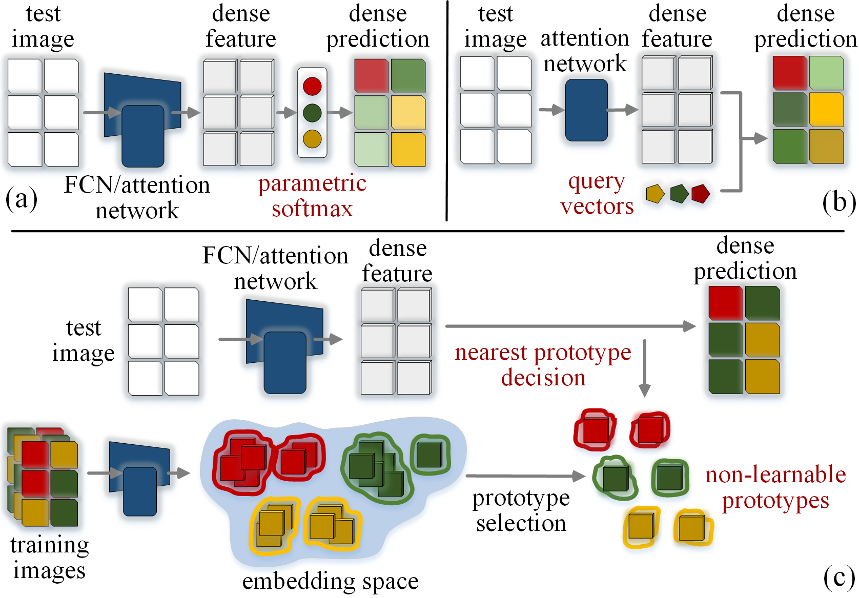
Figure 1: ​Different sematic segmentation paradigms: (a-b) parametric${}_{\!}$ vs${}_{\!}$ (c)${}_{\!}$ nonparametric.${}_{\!}$ Modern${}_{\!}$ segmentation${}_{\!}$ solutions,${}_{\!}$ no matter using (a) parametric softmax or (b) query vectors for mask decoding, can be viewed as learnable prototype based methods that learn class-wise prototypes in a fully parametric manner. We in- stead propose a nonparametric scheme (c) that directly selects subcluster centers of embedded pixels as prototypes, and achieves per-pixel prediction via nonparametric nearest prototype retrieving.

Tackling these two issues can provide insights into modern segmentation model design, and motivate us to rethink the task from a prototype view. The idea of prototype based classification${}_{\!}$ [32] is classical and intuitive (which can date back to the${}_{\!}$ nearest${}_{\!}$ neighbors${}_{\!}$ algorithm${}_{\!}$ [24]${}_{\!}$ and${}_{\!}$ find${}_{\!}$ evi-dence in cognitive science${}_{\!}$ [92, 61]):${}_{\!}$ data samples are classi- fied based on their proximity to representative prototypes of classes. With this perspective, in §2, we first answer question ❶ by pointing out most modern segmentation methods, from softmax based to pixel-query based, from FCN based to attention based, fall into one grand category: parametric models${}_{\!}$ based${}_{\!}$ on learnable${}_{\!}$ prototypes.${}_{\!}$ Consider${}_{\!}$ a${}_{\!}$ segmenta-${}_{\!}$ tion${}_{\!}$ task${}_{\!}$ with${}_{\!}$ $C$${}_{\!}$ semantic${}_{\!}$ classes.${}_{\!}$ Most${}_{\!}$ existing${}_{\!}$ efforts seek to directly learn $C$ class-wise prototypes – softmax weights or query vectors – for parametric, pixel-wise classification. Hence question ❷ becomes more fundamental:${}_{\!}$ ❸${}_{\!}$ What are the limitations of this learnable prototype based parametric paradigm? and ❹${}_{\!}$ How to address these limitations?

${}_{\!}$Driven${}_{\!}$ by${}_{\!}$ question${}_{\!}$ ❸,${}_{\!}$ we${}_{\!}$ find${}_{\!}$ there${}_{\!}$ are${}_{\!}$ three${}_{\!}$ critical${}_{\!}$ limi-
tations:${}_{\!}$ First,${}_{\!}$ usually${}_{\!}$ only${}_{\!}$ one${}_{\!}$ single${}_{\!}$ prototype${}_{\!}$ is${}_{\!}$ learned${}_{\!}$ per class, insufficient to describe rich intra-class variance. The prototypes are simply learned in a fully parametric manner, without considering their representative ability. Second, to map a $H\!\times\!W_{\!}\times_{\!}D_{\!}$ image feature tensor into a $H\!\times\!W_{\!}\times_{\!}C_{\!}$ semantic mask, at${}_{\!}$ least $D\!\times\!C$ parameters${}_{\!}$ are needed for prototype
learning.${}_{\!}$ This${}_{\!}$ hurts${}_{\!}$ generalizability${}_{\!}$ [117],${}_{\!}$ especially${}_{\!}$ in${}_{\!}$ the large-vocabulary case; for instance, if there are $800$ classes and${}_{\!}$ $D_{\!}\!=_{\!}\!512$,${}_{\!}$ we${}_{\!}$ need 0.4M${}_{\!}$ learnable${}_{\!}$ prototype${}_{\!}$ parameters alone.${}_{\!}$ Third,${}_{\!}$ with${}_{\!}$ the${}_{\!}$ cross-entropy${}_{\!}$ loss,${}_{\!}$ only the relative relations between${}_{\!}$ intra-class${}_{\!}$ and${}_{\!}$ inter-class${}_{\!}$ distances${}_{\!}$ are${}_{\!}$ optimized [136, 90, 113]; the actual distances between pixels and prototypes, i.e., intra-class compactness, are ignored${}_{\!}$.

As${}_{\!}$ a${}_{\!}$ response${}_{\!}$ to${}_{\!}$ question${}_{\!}$ ❹,${}_{\!}$ in${}_{\!}$ §3,${}_{\!}$ we${}_{\!}$ develop${}_{\!}$ a${}_{\!}$ nonpa- rametric segmentation framework, based on non-learnable prototypes.${}_{\!\!}$ Specifically,${}_{\!}$ building${}_{\!}$ upon${}_{\!}$ the${}_{\!}$ ideas${}_{\!}$ of${}_{\!}$ prototype
learning${}_{\!}$ [135, 118]${}_{\!}$ and${}_{\!}$ metric${}_{\!}$ learning${}_{\!}$ [41, 65],${}_{\!}$ it${}_{\!}$ is${}_{\!}$ fully aware of the limitations of its parametric counterpart. Inde- pendent${}_{\!}$ of${}_{\!}$ specific${}_{\!}$ backbone${}_{\!}$ architectures${}_{\!}$ (FCN based or attention based), our method is general and brings insights into segmentation model design and training. For model design, our method explicitly sets sub-class centers, in the pixel embedding space, as the prototypes. Each pixel data is predicted${}_{\!}$ to${}_{\!}$ be${}_{\!}$ in${}_{\!}$ the${}_{\!}$ same${}_{\!}$ class${}_{\!}$ as${}_{\!}$ the${}_{\!}$ nearest${}_{\!}$ prototype, without relying on extra learnable parameters. For training, as the prototypes are representative of the dataset, we can directly pose known inductive biases (e.g., intra-class compactness, inter-class separation) as extra optimization criteria and efficiently shape the whole embedding space, instead${}_{\!}$ of${}_{\!}$ optimizing${}_{\!}$ the${}_{\!}$ prediction${}_{\!}$ accuracy${}_{\!}$ only.${}_{\!}$ Our model has three${}_{\!}$ appealing${}_{\!}$ advantages:${}_{\!}$ First,${}_{\!}$ each${}_{\!}$ class${}_{\!}$ is${}_{\!}$ abstracted${}_{\!}$ by${}_{\!}$ a set of prototypes, well capturing class-wise characteristics and intra-class variance. With the clear meaning of the prototypes, the interpretability is also enhanced – the prediction of each pixel can be intuitively understood as the reference of its closest class center in the embedding space [7, 3]. Second, due to the nonparametric nature, the generalizability is improved. Large-vocabulary semantic segmentation can also be handled efficiently, as the amount of learnable prototype parameters is no longer constrained to the number of classes (i.e., 0 vs $D\!\times\!C$). Third, via prototype-anchored metric${}_{\!}$ learning,${}_{\!}$ the${}_{\!}$ pixel${}_{\!}$ embedding${}_{\!}$ space${}_{\!}$ is${}_{\!}$ shaped${}_{\!}$ as${}_{\!}$ well-structured, benefiting segmentation prediction eventually.

${}_{\!}$By${}_{\!}$ answering${}_{\!}$ questions${}_{\!}$ ❶-❹,${}_{\!}$ we${}_{\!}$ formalize${}_{\!}$ prior${}_{\!}$ methods
within a learnable prototype based, parametric framework, and link this field to prototype learning and metric learning. We${}_{\!}$ provide${}_{\!}$ literature${}_{\!}$ review${}_{\!}$ and${}_{\!}$ related${}_{\!}$ discussions${}_{\!}$ in${}_{\!}$ §4.

${}_{\!}$In${}_{\!}$ §5.2,${}_{\!}$ we${}_{\!}$ show${}_{\!}$ our${}_{\!}$ method${}_{\!}$ achieves${}_{\!}$ impressive${}_{\!}$ results${}_{\!}$ over${}_{\!}$ famous${}_{\!}$ datasets${}_{\!}$ (i.e.,${}_{\!}$ ADE20K${}_{\!}$ [142],${}_{\!}$ Cityscapes${}_{\!}$ [23],${}_{\!}$ COCO-Stuff${}_{\!}$ [10])${}_{\!}$ with${}_{\!}$ top-leading${}_{\!}$ FCN based${}_{\!}$ and${}_{\!}$ attention ${}_{\!\!\!}$ based${}_{\!}$ segmentation${}_{\!}$ models${}_{\!}$ (i.e.,${}_{\!}$ HRNet${}_{\!}$ [110], Swin [79],${}_{\!}$ SegFormer${}_{\!}$ [120])${}_{\!}$ and${}_{\!}$ backbones${}_{\!}$ (i.e.,${}_{\!}$ ResNet${}_{\!}$ [46],${}_{\!}$ HRNet [110], Swin${}_{\!}$ [79], MiT${}_{\!}$ [120]). Compared with the paramet-
ric counterparts, our method does not cause any extra computational overhead during testing while reduces the amount${}_{\!}$ of${}_{\!}$ learnable${}_{\!}$ parameters.${}_{\!}$ In${}_{\!}$ §5.3,${}_{\!}$ we${}_{\!}$ demonstrate${}_{\!}$ our${}_{\!}$ method${}_{\!}$ consistently performs well when increasing the number of semantic classes from 150 to 847. Accompanied with a set of ablative studies in §5.4, our extensive experiments verify the power of our idea and the efficacy of our algorithm.

Finally, we draw conclusions in §6. This work is expec- ted to open a new venue for future research in${}_{\!}$ this${}_{\!}$ field.

2 Existing Semantic Segmentation Models as Parametric Prototype Learning

Next we first formalize the existing two mask decoding strategies mentioned in §1, and then answer question ❶ from a unified view of parametric prototype learning.

Parametric Softmax Projection. Almost all FCN-like and many attention-based segmentation models adopt this strategy. Their models comprise two learnable parts: i) an encoder $\phi$ for dense visual feature extraction, and ii) a classifier $\rho$ (i.e., projection head) that projects pixel features into the semantic label space. For each pixel example $i$, its embedding $\bm{i}\!\in\!\mathbb{R}^{D}$, extracted from $\phi$, is fed into $\rho$ for $C$-way classification:

$$p(c|\bm{i})=\frac{\exp(\bm{w}_{c}^{\top}\bm{i})}{\textstyle\sum^{C}_{c^{\prime}=1}\exp(\bm{w}_{c^{\prime}}^{\top}\bm{i})},$$ (1)

where $p(c|\bm{i})\!\in_{\!}\![0,1]$ is the probability that $i$ being assigned to class $c$. $\rho$ is a pixel-wise linear layer, parameterized by $\bm{W}_{\!}\!=\![\bm{w}_{1},\cdots_{\!},\bm{w}_{C}]\!\in\!\mathbb{R}^{C\!\times_{\!}D\!}$; $\bm{w}_{c}\!\in\!\mathbb{R}^{D}$ is a learnable projection vector for $c$-th class; the bias term is omitted for brevity.

Parametric Pixel-Query. A few attention-based segmentation networks [141, 120] work in a more ‘Transformer-like’ manner: given the pixel embedding $\bm{i}\!\in\!\mathbb{R}^{D}$, a set of $C$ query vectors, i.e., $\bm{E}_{\!}\!=\![\bm{e}_{1},\cdots_{\!},\bm{e}_{C}]\!\in\!\mathbb{R}^{C_{\!}\times_{\!}D\!}$, are learned to generate a probability distribution over the $C$ classes:

$$p(c|\bm{i})=\frac{\exp(\bm{e}_{c\!}\ast\bm{i})}{\textstyle\sum^{C}_{c^{\prime}=1}\exp(\bm{e}_{c^{\prime}\!}\ast\bm{i})},$$ (2)

where ‘$\ast$’ is inner product between $\ell_{2}$-normalized inputs.

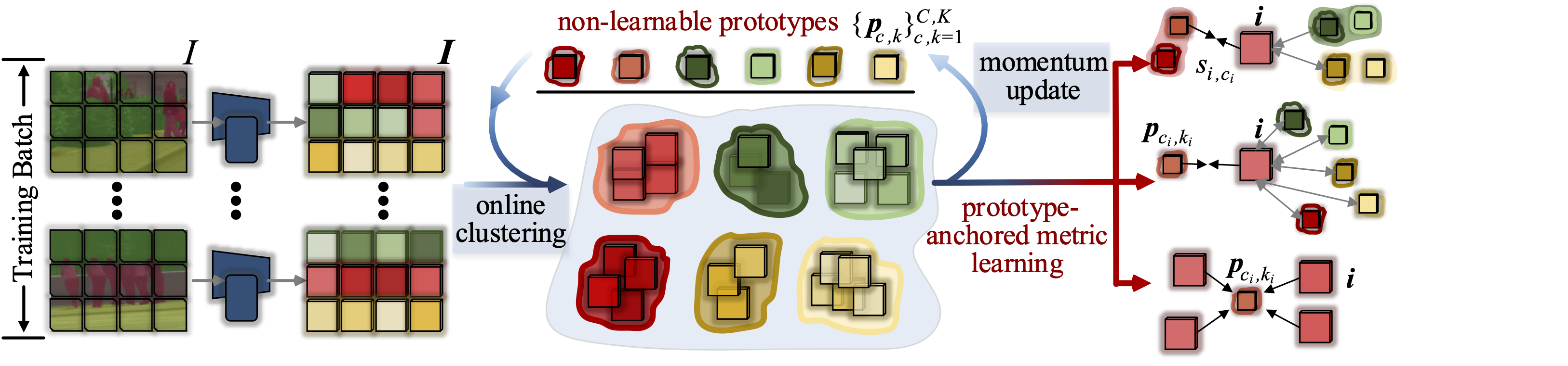
Figure 2: Architecture illustration of our non-learnable prototype based nonparametric segmentation model during the training phase.

Prototype-based Classification. Prototype-based classification [32, 34] has been studied for a long time, dating back to the nearest neighbors algorithm${}_{\!}$ [24] in machine learning and prototype theory${}_{\!}$ [92, 61] in cognitive science. Its prevalence stems from its intuitive idea: represent classes by prototypes, and refer to prototypes for classification. Let $\{p_{m}\}_{m=1\!}^{M}$ be a set of prototypes that are representative of their corresponding classes $\{c_{p_{m}\!\!}\!\in_{\!}\!\{1,\cdots_{\!},C\}\}_{m}$. For a data sample $i$, prediction is made by comparing $i$ with $\{p_{m}\}_{m}$, and taking the class of the winning prototype as response:

$$\hat{c}_{i}=c_{p_{m^{\!*}}},~{}~{}~{}\text{with}~{}~{}~{}m^{*}=\mathop{\arg\min}\limits_{m}\{\langle\bm{i},\bm{p}_{m}\rangle\}_{m=1}^{M},$$ (3)

where $\bm{i}$ and $\{\bm{p}_{m}\}_{m\!}$ are embeddings of the data sample and prototypes in a feature space, and $\langle\cdot,\cdot\rangle$ stands for the distance measure, which is typically set as $\ell_{2}$ distance (i.e., $||\bm{i}\!-\!\bm{p}_{m}||$) [125], yet other proximities can be applied.

Further, Eqs.${}_{\!}$ 1-2 can be formulated in a unified form:

$$p(c|\bm{i})=\frac{\exp(-\langle\bm{i},\bm{g}_{c}\rangle)}{\sum^{C}_{c^{\prime}=1}\exp(-\langle\bm{i},\bm{g}_{c^{\prime}}\rangle)},$$ (4)

where $\bm{g}_{c}\!\in\!\mathbb{R}^{D}$ can be either $\bm{w}_{c}$ in Eq. 1 or $\bm{e}_{c}$ in Eq. 2.

${}_{\!}$With${}_{\!}$ Eqs.${}_{\!}$ 3-4,${}_{\!}$ we${}_{\!}$ are${}_{\!}$ ready${}_{\!}$ to${}_{\!}$ answer${}_{\!}$ questions${}_{\!}$ ❶❷.${}_{\!}$ Both the two types of methods are based on learnable prototypes; they are parametric models in the sense that they learn one prototype $\bm{g}_{c}$, i.e., linear weight $\bm{w}_{c}$ or query vector $\bm{e}_{c}$, for each${}_{\!}$ class${}_{\!}$ $c$${}_{\!}$ (i.e.,${}_{\!}$ $M_{\!}\!=_{\!}\!C\!~{}$).${}_{\!}$ Thus${}_{\!}$ one${}_{\!}$ can${}_{\!}$ consider${}_{\!}$ softmax${}_{\!}$ pro- jection based methods ‘secretly’ learn the query vectors. As
for the difference, in addition to different distance measures (i.e., inner product vs cosine similarity), pixel-query based methods [141, 120] can feed the queries into cross-attention decoder layers for cross-class context exchanging, rather than softmax projection based counterparts only leveraging the learned class weights within the softmax layer.

With the unified view of parametric prototype learning, a few intrinsic yet long ignored issues in this field unfold:

First, prototype selection [37] is a vital aspect in the design of a prototype based learner – prototypes should be typical for their classes. Nevertheless, existing semantic segmentation algorithms often describe each class by only one prototype, bearing no intra-class variation. Moreover, the prototypes are directly learned in a fully parametric manner, without accounting for their representative ability.

${}_{\!}$Second,${}_{\!}$ the${}_{\!}$ amount${}_{\!}$ of${}_{\!}$ the${}_{\!}$ learnable${}_{\!}$ prototype${}_{\!}$ parameters, i.e.,${}_{\!}$ $\{\bm{g}_{c\!}\!\in_{\!}\!\mathbb{R}^{D}\}_{c=1}^{C}$, grows with the number of classes. This may hinder the scalability, especially when a large number of classes are present. For example, if there are 800 classes and the pixel feature dimensionality is 512, at least 0.4M parameters are needed for prototype learning alone, making large-vocabulary segmentation a hard task. Moreover, if we want to represent each class by ten prototypes, instead of only one, we need to learn 4M prototype parameters.

${}_{\!}$Third,${}_{\!}$ Eq.${}_{\!}$ 3${}_{\!}$ intuitively${}_{\!}$ shows${}_{\!}$ that${}_{\!}$ prototype based${}_{\!}$ learners make metric comparisons of data${}_{\!}$ [8]. However, existing algorithms often supervise dense segmentation representation by directly optimizing the accuracy of pixel-wise prediction (e.g., cross-entropy loss), ignoring known inductive biases${}_{\!}$ [85, 84], e.g., intra-class compactness, about the feature distribution. This will hinder the discrimination potential of the learned segmentation features, as suggested by many literature in representation learning ${}_{\!}$ [77, 97, 116].

${}_{\!}$After${}_{\!}$ tackling${}_{\!}$ question${}_{\!}$ ❸,${}_{\!}$ in${}_{\!}$ the${}_{\!}$ next${}_{\!}$ section${}_{\!}$ we${}_{\!}$ will${}_{\!}$ detail${}_{\!}$
our${}_{\!}$ non-learnable${}_{\!}$ prototype${}_{\!}$ based${}_{\!}$ nonparametric${}_{\!}$ segmenta- tion method, which serves as a solid response to question${}_{\!}$ ❹.

3 Non-Learnable Prototype based Nonparametric Semantic Segmentation

We build a nonparametric segmentation framework that${}_{\!}$ conducts${}_{\!}$ dense${}_{\!}$ prediction${}_{\!}$ by${}_{\!}$ a${}_{\!}$ set${}_{\!}$ of${}_{\!}$ non-learnable${}_{\!}$ class${}_{\!}$ pro- totypes,${}_{\!}$ and${}_{\!}$ directly${}_{\!}$ supervises${}_{\!}$ the${}_{\!}$ pixel${}_{\!}$ embedding${}_{\!}$ space${}_{\!}$ via a prototype-anchored${}_{\!}$ metric${}_{\!}$ learning scheme (Fig.${}_{\!}$ 2).

Non-Learnable${}_{\!}$ Prototype${}_{\!}$ based${}_{\!}$ Pixel${}_{\!}$ Classification.${}_{\!}$ As normal,${}_{\!}$ an${}_{\!}$ encoder${}_{\!}$ network${}_{\!}$ (FCN${}_{\!}$ based${}_{\!}$ or${}_{\!}$ attention based), i.e., $\phi$, is first adopted to map the input image $I_{\!}\!\in_{\!}\!\mathbb{R}^{h_{\!}\times_{\!}w_{\!}\times_{\!}3\!}$, to a 3D feature tensor $\bm{I}_{\!}\!\in_{\!}\!\mathbb{R}^{H_{\!}\times_{\!}W_{\!}\times_{\!}D\!}$. For pixel-wise $C$-way classification, rather than prior semantic segmentation models that automatically learn $C$ class weights $\{\bm{w}_{c\!}\!\in_{\!}\!\mathbb{R}^{D\!}\}_{c=1\!}^{C}$ (cf.${}_{\!}$ Eq.${}_{\!}$ 1) or $C$ queries vectors $\{\bm{e}_{c\!}\!\in_{\!}\!\mathbb{R}^{D\!}\}_{c=1\!}^{C}$ (cf.${}_{\!}$ Eq.${}_{\!}$ 2), we refer to a group of $CK$ non-learnable prototypes, i.e., $\{\bm{p}_{c,k\!}\!\in\!\mathbb{R}^{D\!}\}_{c,k=1}^{C,K}$, which${}_{\!}$ are${}_{\!}$ based${}_{\!}$ solely${}_{\!}$ on class data sub-centers. More specifically, each class $c\!\in\!\{1,\cdots_{\!},C\}$ is represented by a total of $K$ prototypes $\{\bm{p}_{c,k\!}\}_{k=1}^{K}$, and prototype $\bm{p}_{c,k}$ is determined as the center of $k$-th sub-cluster of training pixel samples belonging to class $c$, in the embedding space $\phi$. In this way, the prototypes can comprehensively capture characteristic properties of the corresponding classes, without introducing extra learnable parameters outside $\phi$. Analogous to Eq.${}_{\!}$ 3, the category prediction of each pixel $i\!\in\!I$ is achieved by a winner-take-all classification:

$$\hat{c}_{i}=c^{*},~{}~{}\text{with}~{}~{}(c^{*},k^{*})=\mathop{\arg\min}\limits_{(c,k)}\{\langle\bm{i},\bm{p}_{c,k}\rangle\}_{c,k=1}^{C,K},$$ (5)

where $\bm{i}\!\in\!\mathbb{R}^{D\!}$ stands for the $\ell_{2}$-normalized embedding of pixel $i$, i.e., $\bm{i}\!\in_{\!}\!\bm{I}$, and the distance measure${}_{\!}$ $\langle\cdot,\cdot\rangle$${}_{\!}$ is defined as the negative cosine similarity, i.e.,${}_{\!}$ $\langle\bm{i},\bm{p}\rangle\!=\!-\bm{i}^{\top\!}\bm{p}$.

With this exemplar-based reasoning mode, we first define the probability distribution of pixel $i$ over the $C$ classes:

$$\!\!\!\!\!p(c|\bm{i})\!=\!\frac{\exp(-s_{i,c})}{\sum^{C}_{c^{\prime}=1\!}\exp(-s_{i,c^{\prime}\!})},~{}~{}\text{with}~{}~{}s_{i,c}\!=\!\min\{\langle\bm{i},\bm{p}_{c,k}\rangle\}_{k=1}^{K},$$ (6)

where the pixel-class distance $s_{i,c}\!\in_{\!}\![-1,1]$ is computed as the distance to the closest prototype of class $c$. Given the groundtruth class of each pixel $i$, i.e., $c_{i}\!\in\!\{1,\cdots_{\!},C\}$, the cross-entropy loss can be therefore used for training:

$$\mathcal{L}_{\text{CE}} =-\log p(c_{i}|\bm{i})$$ (7)

$$=-\log\frac{\exp(-s_{i,c_{i}})}{\exp(-s_{i,c_{i}})\!+\!\sum_{c^{\prime}\!\neq c_{i}\!}\exp(-s_{i,c^{\prime}})}.\!\!$$

In our case, Eq.${}_{\!}$ 7 can be viewed as pushing pixel $i$ closer to the nearest prototype of its corresponding class, i.e., $c_{i}$, and further from other close prototypes of irrelevant classes, i.e., $c^{\prime}\!\neq c_{i}$. However, only adopting such training objective is not enough, due to two reasons. First, Eq.${}_{\!}$ 7 only considers

pixel-class distances, e.g., $s_{i,c}$, without addressing within-class pixel-prototype relations, e.g., $\langle\bm{i},\bm{p}_{c_{i},k}\rangle$. For example,

for discriminative representation learning, pixel $i$ is expec- ted to be pushed further close to a certain prototype (i.e., a particularly suitable pattern) of class $c_{i}$, and, distant from other prototypes (i.e., other irrelevant but within-class patterns) of class $c_{i}$. Eq.${}_{\!}$ 7 cannot capture this nature. Second,

as the pixel-class distances are normalized across all classes

(cf.${}_{\!}$ Eq.${}_{\!}$ 6),${}_{\!}$ Eq.${}_{\!}$ 7${}_{\!}$ only${}_{\!}$ optimizes${}_{\!}$ the${}_{\!}$ relative${}_{\!}$ relations${}_{\!}$ between${}_{\!}$

intra-class (i.e., $s_{i,c_{i}}$) and inter-class (i.e., $\{s_{i,c^{\prime}\!}\}_{c^{\prime}\!\neq c_{i}}$) distances, instead of directly regularizing the cosine distances between pixels and classes. For example, when the intra-class distance $s_{i,c_{i}}$ of pixel $i$ is relatively smaller than other inter-class distances $\{s_{i,c^{\prime}}\}_{c^{\prime}\!\neq c_{i}}$, the penalty from Eq.${}_{\!}$ 7 will be small, but the intra-class distance $s_{i,c_{i}\!}$ might still be large [136, 90]. Next we first elaborate on our within-class online clustering strategy and then detail our two extra training objectives which rely on prototype assignments (i.e., clustering results) and address the above two issues respectively.

Within-Class Online Clustering. We approach online clu- stering for prototype selection and assignment: pixel samples within the same class are assigned to the prototypes belonging to that class, and the prototypes are then updated according to the assignments. Clustering imposes a natural bottleneck [56] that forces the model to discover intra-class discriminative patterns yet discard instance-specific details. Thus the prototypes, selected as the sub-cluster centers, are typical of the corresponding classes. Conducting clustering online makes our method scalable to large amounts of data, instead of offline clustering requiring multiple passes over the entire dataset for feature computation [13].

Formally, given pixels $\mathcal{I}^{c}\!=\!\{i_{n}\}_{n=1\!}^{N}$ in a training batch that belong to class $c$ (i.e.,${}_{\!}$ $c_{i_{n}\!}\!=\!c$), our goal is to map the pixels $\mathcal{I}^{c}$ to the $K$ prototypes $\{\bm{p}_{c,k\!}\}_{k=1\!}^{K}$ of class $c$. We denote this pixel-to-prototype mapping as $\bm{L}^{c\!}\!=\![\bm{l}_{i_{n}}]_{n=1\!}^{N}\!\in\!\{0,1\}^{K\times N}$, where $\bm{l}_{i_{n}\!}\!=\![l_{i_{n},k}]_{k=1\!}^{K}\!\in\!\{0,1\}^{K}$ is the one-hot assignment vector of pixel $i_{n}$ over the $K$ prototypes. The optimization of $\bm{L}^{c\!}$ is achieved by maximizing the similarity between pixel embeddings, i.e., $\bm{X}^{c\!}\!=\![\bm{i}_{n}]_{n=1\!}^{N}\!\in\!\mathbb{R}^{D\times N}$, and the prototypes, i.e., $\bm{P}^{c\!}\!=\![\bm{p}_{c,k}]_{k=1\!}^{K}\!\in\!\mathbb{R}^{D\times K}$:

$$\!\!\!\!\!\!\!\!\max_{\bm{L}^{c}}\texttt{Tr}(\bm{L}^{c\top\!}\bm{P}^{c\top\!}\bm{X}^{c}),$$ (8)

$$\textit{s.t.}~{}~{}~{}~{}\bm{L}^{c\!}\!\in\!\{0,1\}^{K\times N}, ~{}\bm{L}^{c\top}\bm{1}^{K}=\bm{1}^{N},\bm{L}^{c}\bm{1}^{N}=\frac{N}{K}\bm{1}^{K},$$

where $\bm{1}^{K\!}$ denotes the vector of all ones of $K$ dimensions. The unique assignment constraint, i.e., $\bm{L}^{c\top}\bm{1}^{K\!}\!=_{\!}\!\bm{1}^{N}$, ensures that each pixel is assigned to one and only one prototype. The equipartition constraint, i.e., $\bm{L}^{c}\bm{1}^{N\!}\!=\!\frac{N}{K}\bm{1}^{K}$, enforces that on average each prototype is selected at least $\frac{N}{K}$ times in the batch${}_{\!}$ [13]. This prevents the trivial solution: all pixel samples are assigned to a single prototype, and eventually benefits the representative ability of the prototypes. To solve Eq.${}_{\!}$ LABEL:eq:nc1, one can relax $\bm{L}^{c}$ to be an element of the transportation polytope${}_{\!}$ [25, 2]:

$$\!\!\!\!\!\!\!\!\!\!\!\!\!\!\!\!\max_{{\bm{L}}^{c}}\texttt{Tr}({\bm{L}}^{c\top\!}\bm{P}^{c\top\!}\bm{X}^{c})+\kappa\!~{}h(\bm{L}^{c}),$$ (9)

$$\textit{s.t.}~{}~{}~{}~{}{\bm{L}}^{c\!}\!\in\!\mathbb{R}^{K\times N}_{+} ,~{}{\bm{L}}^{c\top}\bm{1}^{K}=\bm{1}^{N},{\bm{L}}^{c}\bm{1}^{N}=\frac{N}{K}\bm{1}^{K},$$

where $h(\bm{L}^{c})_{\!}\!=_{\!}\!\sum_{n,k\!}-l_{i_{n},k}\log l_{i_{n},k\!}$ is an entropy, and $\kappa\!>\!0$ is a parameter that controls the smoothness of distribution. With the soft assignment relaxation and the extra regularization term $h(\bm{L}^{c})$, the solver of Eq. LABEL:eq:nc2 can be given as${}_{\!}$ [25]:

$${\bm{L}}^{c}=\texttt{diag}(\bm{u})\exp\big{(}\frac{\bm{P}^{c\top\!}\bm{X}^{c}}{\kappa}\big{)}\texttt{diag}(\bm{v}),$$ (10)

where $\bm{u}\!\in\!\mathbb{R}^{K\!}$ and $\bm{v}\!\in\!\mathbb{R}^{N\!}$ are renormalization vectors, computed by few steps of Sinkhorn-Knopp iteration [25]. Our online clustering is highly efficient on GPU, as it only involves a couple of matrix multiplications; in practice, clustering $10$K pixels into $10$ prototypes takes only $2.5$ ms.

Pixel-Prototype Contrastive Learning. With the assign- ment probability matrix ${\bm{L}}^{c\!}\!=\![{\bm{l}}_{i_{n}}]_{n=1\!}^{N}\!\in\![0,1]^{K\times N}$, we online group the training pixels $\mathcal{I}^{c\!}\!=\!\{i_{n}\}_{n=1\!}^{N}$ into $K$ prototypes $\{\bm{p}_{c,k\!}\}_{k=1\!}^{K}$ within class $c$. After all the samples in current batch are processed, each pixel $i$ is assigned to $k_{i}$-th prototype of class $c_{i}$, where $k_{i}\!=\!\arg\max_{k}\{{l}_{i,k}\}_{k=1}^{K}$ and ${l}_{i,k}\!\in\!{\bm{l}}_{i}$. It is natural to derive a training objective for prototype assignment prediction, i.e., maximize the prototype assignment posterior probability. This can be viewed as a pixel-prototype contrastive learning strategy, and addresses

the first limitation of Eq. 7:

$$\!\!\!\mathcal{L}_{\text{PPC}}\!=\!-\!\log\frac{\exp(\bm{i}^{\top}\!\bm{p}_{c_{i},k_{i}}/\tau)}{\exp(\bm{i}^{\top}\!\bm{p}_{c_{i},k_{i}\!}/\tau)\!+\!\sum_{\bm{p}^{-}\in\mathcal{P}^{-}\!}\exp(\bm{i}^{\top}\!\bm{p}^{-}/\tau)},$$ (11)

where $\mathcal{P}^{-\!}\!=\!\{\bm{p}_{c,k}\}_{c,k=1}^{C,K}\big{/}\bm{p}_{c_{i},k_{i}}$, and the temperature $\tau$ controls the concentration level of representations. Intuitively, Eq. 11 enforces each pixel embedding $\bm{i}$ to be similar with its${}_{\!}$ assigned${}_{\!}$ (‘positive’)${}_{\!}$ prototype${}_{\!}$ $\bm{p}_{c_{i},k_{i}}$,${}_{\!}$ and${}_{\!}$ dissimilar${}_{\!}$ with other $CK\!-\!1$ irrelevant (‘negative’) prototypes $\mathcal{P}^{-}$. Compared with prior pixel-wise metric learning based segmentation models [113], which consume numerous negative pixel samples, our method only needs $CK$ prototypes for pixel-prototype contrast computation, neither causing large memory cost nor requiring heavy pixel pair-wise comparison.

Pixel-Prototype${}_{\!}$ Distance${}_{\!}$ Optimization.${}_{\!}$ Building${}_{\!}$ upon${}_{\!}$ the relative comparison over pixel-class/-prototype distances, Eq.${}_{\!}$ 7${}_{\!}$ and Eq.${}_{\!}$ 11 inspire inter-class/-cluster discrinimitive- ness, but less consider reducing the intra-cluster variation, i.e., making pixel features of the same prototype compact. Thus a compactness-aware loss is used for further regulari- zing representations by directly minimizing the distance be- tween${}_{\!}$ each${}_{\!}$ embedded${}_{\!}$ pixel${}_{\!}$ and${}_{\!}$ its${}_{\!}$ assigned${}_{\!}$ prototype:

$$\!\!\!\mathcal{L}_{\text{PPD}}\!=\!(1-\bm{i}^{\top\!}\bm{p}_{c_{i},k_{i}})^{2}.$$ (12)

Note that both $\bm{i}$ and $\bm{p}_{c_{i},k_{i}\!}$ are $\ell_{2}$-normalized. This training objective minimizes intra-cluster variations while maintaining separation between features with different prototype assignments, making our model more robust against outliers.

Network Learning and Prototype Update. Our model is a nonparametric approach that learns semantic segmentation by directly optimizing the pixel embedding space $\phi$. It is called nonparametric because it constructs prototype hypotheses directly from the training pixel samples themselves. Thus the parameters of the feature extractor $\phi$ are learned through stochastic gradient descent, by minimizing the combinatorial loss over all the training pixel samples:

$$\mathcal{L}_{\text{SEG}}=\mathcal{L}_{\text{CE}}+\lambda_{1}\mathcal{L}_{\text{PPC}}+\lambda_{2}\mathcal{L}_{\text{PPD}}.$$ (13)

Meanwhile, the non-learnable prototypes $\{\bm{p}_{c,k}\}_{c,k=1\!}^{C,K}$ are not learned by stochastic gradient descent, but are computed as the centers of the corresponding embedded pixel samples. To do so, we let the prototypes evolve continuously by accounting for the online clustering results. Particularly, after each training iteration, each prototype is updated as:

$$\bm{p}_{c,k}\leftarrow\mu\bm{p}_{c,k}+(1-\mu)\bar{\bm{i}}_{c,k},$$ (14)

where $\mu\!\in\![0,1]$ is a momentum coefficient, and $\bar{\bm{i}}_{c,k}$ indicates the $\ell_{2}$-normalized, mean vector of the embedded training pixels, which are assigned to prototype $\bm{p}_{c,k}$ by online clustering. With the clear meaning of the prototypes, our segmentation procedure can be intuitively understood as retrieving the most similar prototypes (sub-class centers). Fig. 3 provides prototype retrieval results for person and car with $K\!=\!3$ prototypes for each. The prototypes are associ-

ated with different colors (i.e., red, green, and blue). For each pixel, its distance to the closest prototype is visualized using the corresponding prototype color. As can be seen, the prototypes well correspond to meaningful patterns within classes, validating their representativeness.

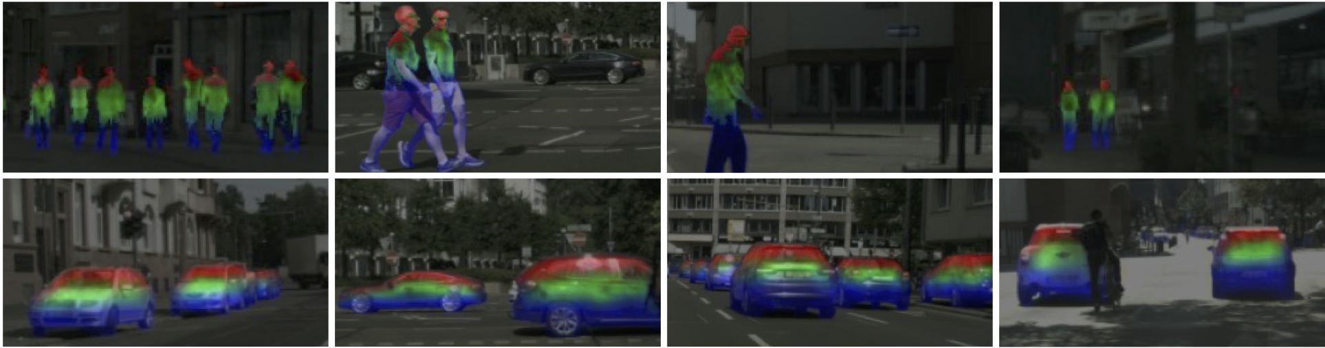
Figure 3: Visualization of pixel-prototype similarity for person (top) and car (bottom) classes. Please refer to §3 for details.

4 Related Work

In this section, we review representative work in semantic segmentation, prototype learning and metric learning.

Semantic Segmentation. Recent years have witnessed remarkable progress in semantic segmentation, due to${}_{\!}$ the${}_{\!}$ fast evolution of backbone architectures ${}_{\!}$–${}_{\!}$ from${}_{\!}$ CNN-based${}_{\!}$ (e.g.,${}_{\!}$ VGG${}_{\!}$ [99],${}_{\!}$ ResNet${}_{\!}$ [46])${}_{\!}$ to${}_{\!}$ Transformer-like${}_{\!}$ [107]${}_{\!}$ (e.g.,${}_{\!}$ ViT
[31], Swin${}_{\!}$ [79]), and${}_{\!}$ segmentation${}_{\!}$ models ${}_{\!}$–${}_{\!}$ from FCNs [80] to attention networks (e.g.,${}_{\!}$ SegFormer${}_{\!}$ [120]).${}_{\!}$ Specifically,${}_{\!}$ FCN${}_{\!}$ [80]${}_{\!}$ is${}_{\!}$ a${}_{\!}$ milestone;${}_{\!}$ it learns dense prediction efficiently.
Since it was proposed, numerous efforts have been devoted
to improving FCN, by, for example, enlarging the receptive${}_{\!}$ field [137, 26, 126, 130, 15, 16]; strengthening context cues [91, 140, 130, 4, 78, 71, 82, 134, 44, 49, 131, 128, 76, 48, 58, 57, 143]; leveraging boundary information [14, 129, 28, 6, 67, 133, 139];${}_{\!}$ incorporating${}_{\!}$ neural${}_{\!}$ attention [42, 114, 64, 138, 50, 112, 43, 69, 35, 51, 103]; or automating network engineering [18, 73, 86, 70]. Lately,${}_{\!}$ Transfor- mer based${}_{\!}$ solutions${}_{\!}$ [120, 102, 141, 20] attained growing attention; enjoying the flexibility in long-range dependency modeling, fully attentive solutions yield impressive results.

Different from current approaches that are typically built upon${}_{\!}$ learnable${}_{\!}$ prototypes,${}_{\!}$ in${}_{\!}$ pre-deep${}_{\!}$ era,${}_{\!}$ many${}_{\!}$ segmenta- tion systems are nonparametric [81, 104, 105, 74, 75, 33]. By absorbing their case-based reasoning ideas, we build a nonparametric segmentation network, which explicitly derives prototypes from sample clusters and hence directly optimizes the embedding space with distance metric constraints. In [63, 113], while cluster-/pixel-level metric loss is adopted to regularize representation, the pixel class is still inferred via parametric softmax. [54] purely relies on class
embeddings,${}_{\!}$ which,${}_{\!}$ however,${}_{\!}$ are${}_{\!}$ fully${}_{\!}$ trainable.${}_{\!}$ Thus${}_{\!}$ [63, 113, 54] are all parametric methods. As far as we know, [53]
is${}_{\!}$ the${}_{\!}$ only${}_{\!}$ non-learnable${}_{\!}$ prototype,${}_{\!}$ deep${}_{\!}$ learning${}_{\!}$ based${}_{\!}$ se- mantic${}_{\!}$ segmentation${}_{\!}$ model.${}_{\!}$ But${}_{\!}$ [53] treats image regions as prototypes, incurring huge memory and computational demand. Besides, [53] only considers the relative difference between inter-and intra-class sample-prototype distances like the parametric counterparts. Our method is more principled with fewer heuristic${}_{\!}$ designs.${}_{\!}$ Unlike${}_{\!}$ [53],${}_{\!}$ we represent prototypes as sub-cluster centers and obtain online assignments, allowing our method to scale gracefully to any
dataset size. We encourage a sparse distance distribution with compactness-awareness, reinforcing the embedding discrimination.${}_{\!}$ With${}_{\!}$ a${}_{\!}$ broader${}_{\!}$ view,${}_{\!}$ a${}_{\!}$ few${}_{\!}$ embedding based instance segmentation approaches [27, 87] can be viewed as nonparametric, i.e., treat instance centroids as prototypes.

Prototype Learning. Cognitive psychological studies evi- dence that people use past cases as models when learning to
solve problems${}_{\!}$ [88, 1, 127]. Among various machine learning algorithms, ranging from classical statistics based methods to Support Vector Machine to Multilayer Perceptrons${}_{\!}$ [32, 98, 34, 9], prototype based classification gains particular interest, due to its exemplar-driven nature and intuitive interpretation:${}_{\!}$ observations${}_{\!}$ are${}_{\!}$ directly${}_{\!}$ compared${}_{\!}$ with re- presentative examples. Based on the nearest neighbors rule – the earliest prototype learning method${}_{\!}$ [24], many famous, nonparametric classifiers are proposed${}_{\!}$ [37], such as Learning Vector Quantization (LVQ) [62], generalized LVQ${}_{\!}$ [96], and Neighborhood Component Analysis${}_{\!}$ [38, 94]. There has been${}_{\!}$ a${}_{\!}$ recent${}_{\!}$ surge${}_{\!}$ of${}_{\!}$ interest${}_{\!}$ to${}_{\!}$ integrate${}_{\!}$ deep${}_{\!}$ learning${}_{\!}$ into prototype${}_{\!}$ learning,${}_{\!}$ showing${}_{\!}$ good${}_{\!}$ potential${}_{\!}$ in${}_{\!}$ few-shot [100], zero-shot${}_{\!}$ [55],${}_{\!}$ and${}_{\!}$ unsupervised${}_{\!}$ learning${}_{\!}$ [118, 122],${}_{\!}$ as${}_{\!}$ well${}_{\!}$ as${}_{\!}$ supervised${}_{\!}$ classification${}_{\!}$ [117, 125, 39, 84]${}_{\!}$ and${}_{\!}$ interpretable${}_{\!}$ networks${}_{\!}$ [66].${}_{\!}$ Remarkably,${}_{\!}$ as${}_{\!}$ many${}_{\!}$ few-shot segmentation models can be viewed as prototype-based networks [108, 30, 111], our work sheds light on the possibility of closer collaboration between the two segmentation fields.

Metric Learning. The selection of proper distance measure${}_{\!}$ impacts${}_{\!}$ the${}_{\!}$ success of prototype based learners${}_{\!}$ [8]; metric learning and prototype learning are naturally related. As the literature on metric learning is vast [59], only the most relevant ones are discussed. The goal of metric learning is to learn a distance metric/embedding such that similar samples are pulled together and dissimilar samples are pushed away. It has shown a significant benefit by learning deep representation using metric loss functions (e.g., contrastive loss [41], triplet loss [97], $n$-pair loss${}_{\!}$ [101]) for applications (e.g., image retrieval [109], face recognition [97]). Recently, metric
learning showed good potential in unsupervised representa- tion learning.${}_{\!}$ Specifically,${}_{\!}$ many${}_{\!}$ instance-based${}_{\!}$ approaches use the contrastive loss [40, 89] to explicitly compare pairs of image representations, so as to push away features from different images while pulling together those from transformations of the same image [89, 47, 19, 17, 45]. Since computing all the pairwise comparisons on a large dataset is challenging, some clustering-based methods turn to discriminate between groups of images with similar features instead of individual images [5, 121, 12, 124, 13, 65, 2, 106, 123]. Our prototype-anchored metric learning strategy shares a similar spirit of posing metric constraints over prototype (cluster) assignments, but it is to reshape the pixel segmentation embedding space with explicit supervision.

5 Experiment

5.1 Experimental Setup

Datasets. Our experiments are conducted on three datasets:​​

• ADE20K [142] is a large-scale scene parsing benchmark that covers $150$ stuff/object categories. The dataset is divided into 20k/2k/3k images for train/val/test.

• Cityscapes [23] has 5k finely annotated urban scene images, with $2,\!975/500/1,\!524$ for train/val/test. The segmentation performance is evaluated over $19$ challenging categories, such as rider, bicycle, and traffic light.

• COCO-Stuff [10] has 10k images gathered from COCO [72], with 9k and 1k for train and test, respectively. There are 172 semantic categories in total, including 80 objects, 91 stuffs and 1 unlabeled.

Training. Our method is implemented on MMSegmentation [22], following default training settings. In particular, all backbones are initialized using corresponding weights pre-trained on ImageNet-1K [93], while remaining layers are randomly initialized. We use standard data augmentation techniques, including random scale jittering with a factor in $[0.5,2]$, random horizontal flipping, random cropping as well as random color jittering. We train models using SGD/AdamW for FCN-/attention-based models, respectively. The learning rate is scheduled following the polynomial annealing policy. In addition, for Cityscapes, we use a batch size of $8$, and a training crop size of $768\!\times\!768$. For ADE20K and COCO-Stuff, we use a crop size of $512\!\times\!512$ and train the models with batch size $16$. The models are trained for $160$k, $160$k, and $80$k iterations on Cityscapes, ADE20K and COCO-Stuff, respectively. Exceptionally, for ablation study, we train models for 40K iterations. The hyper-parameters are empirically set to: $K\!=\!10$, $m\!=\!0.999$, $\tau\!=\!0.1$, $\kappa\!=\!0.05$, $\lambda_{1}\!=\!0.01$, $\lambda_{2}\!=\!0.01$.

Testing. For ADE20K and COCO-Stuff, we rescale the short scale of the image to training crop size, with the aspect ratio kept unchanged. For Cityscapes, we adopt sliding window inference with the window size $768\times 768$. For simplicity, we do not apply any test-time data augmentation. Our model is implemented in PyTorch and trained on eight Tesla V100 GPUs with a 32GB memory per-card. Testing is conducted on the same machine.

Baselines. We mainly compare with four widely recognized segmentation models, i.e., two FCN based (i.e., FCN [80], HRNet [110]) and two attention based (i.e., Swin [79] and SegFormer [120]). For fair comparison, all the models are based on our reproduction, following the hyper-parameter and augmentation recipes used in MMSegmentation [22].

Evaluation Metric. Following conventions [80, 15], mean intersection-over-union (mIoU) is adopted for evaluation.

Method				Backbone	# Param (M)	mIoU (%)
DeepLabV3+ [ECCV18] [16]	ResNet-101 [46]	62.7	44.1
OCR [ECCV20] [131]	HRNetV2-W48 [110]	70.3	45.6
MaskFormer [NeurIPS21] [20]	ResNet-101 [46]	60.0	46.0
UperNet [ECCV20] [119]	Swin-Base [79]	121.0	48.4
OCR [ECCV20] [131]	HRFormer-B [132]	70.3	48.7
SETR [CVPR21] [141]	ViT-Large [31]	318.3	50.2
Segmenter [ICCV21] [102]	ViT-Large [31]	334.0	51.8
†MaskFormer [NeurIPS21] [20]	Swin-Base [79]	102.0	52.7
FCN [CVPR15] [80]		68.6	39.9
Ours	ResNet-101 [46]	68.5	41.1 $\uparrow$ 1.2
HRNet [PAMI20] [110]		65.9	42.0
Ours	HRNetV2-W48 [110]	65.8	43.0 $\uparrow$ 1.0
Swin [ICCV21] [79]		90.6	48.0
Ours	Swin-Base [79]	90.5	48.6 $\uparrow$ 0.6
SegFormer [NeurIPS21] [120]		64.1	50.9
Ours	MiT-B4 [120]	64.0	51.7 $\uparrow$ 0.8

 ^†: backbone is pre-trained on ImageNet-22K.

Table 1: Quantitative results (§5.2) on ADE20K${}_{\!}$ [142] val.

Method				Backbone	# Param (M)	mIoU (%)
PSPNet [CVPR17] [137]	ResNet-101 [46]	65.9	78.4
PSANet [ECCV18] [138]	ResNet-101 [46]	-	78.6
AAF [ECCV18] [60]	ResNet-101 [46]	-	79.1
Segmenter [ICCV21] [102]	ViT-Large [31]	322.0	79.1
ContrastiveSeg [ICCV21] [113]	ResNet-101 [46]	58.0	79.2
MaskFormer [NeurIPS21] [20]	ResNet-101 [46]	60.0	80.3
DeepLabV3+ [ECCV18] [16]	ResNet-101 [46]	62.7	80.9
OCR [ECCV20] [131]	HRNetV2-W48 [110]	70.3	81.1
FCN [CVPR15] [80]		68.6	78.1
Ours	ResNet-101 [46]	68.5	79.1 $\uparrow$ 1.0
HRNet [PAMI20] [110]		65.9	80.4
Ours	HRNetV2-W48 [110]	65.8	81.1 $\uparrow$ 0.7
Swin [ICCV21] [79]		90.6	79.8
Ours	Swin-Base [79]	90.5	80.6 $\uparrow$ 0.8
SegFormer [NeurIPS21] [120]		64.1	80.7
Ours	MiT-B4 [120]	64.0	81.3 $\uparrow$ 0.6

Table 2: Quantitative results (§5.2) on Cityscapes [23] val.

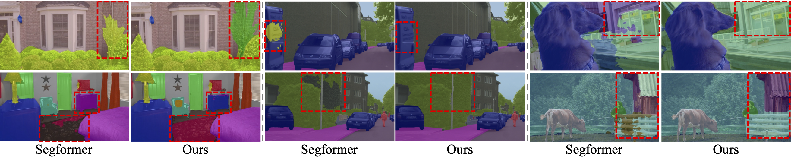
Figure 4: Qualitative results of Segformer [120] and our approach (from left to right: ADE20K [142], Cityscapes [23], COCO-Stuff [10]).

5.2 Comparison to State-of-the-Arts

ADE20K [142] val. Table 1 reports comparisons with representative models on ADE20K val. Our nonparametric scheme obtains consistent improvements over the baselines, with fewer learnable parameters. In particular, it yields 1.2% and 1.0% mIoU improvements over the FCN-based counterparts, i.e., FCN [80] and HRNet [110]. Similar performance gains (0.6% and 0.8%) are obtained over recent attention-based models, i.e., Swin [79] and SegFormer [120], manifesting the high versatility of our approach.

Cityscapes [23] val. Table 6 shows again our compelling performance on Cityscapes val. Specifically, our approach surpasses all the competitors, i.e., 1.0% over FCN, 0.7% over HRNet, 0.8% over Swin, and 0.6% over Segformer.

COCO-Stuff [10] test. As listed in Table 3, our approach also demonstrates promising performance on COCO-Stuff test. It outperforms all the baselines. Notably, with MiT-B4 [120] as the network backbone, our approach earns an mIoU score of 43.3%, establishing a new state-of-the-art.

Qualitative Results. Fig. 4 provides qualitative comparison of Ours against Segformer [120] on representative examples in the three datasets. We observe that our approach is able to handle diverse challenging scenarios and produce more accurate results (as highlighted in red dashed boxes).

Method				Backbone	# Param (M)	mIoU (%)
SVCNet [CVPR19] [29]	ResNet-101 [46]	-	39.6
DANet [CVPR19] [35]	ResNet-101 [46]	69.1	39.7
SpyGR [CVPR20] [68]	ResNet-101 [46]	-	39.9
MaskFormer [NeurIPS21] [20]	ResNet-101 [46]	60.0	39.8
ACNet [ICCV19] [36]	ResNet-101 [46]	-	40.1
OCR [ECCV20] [131]	HRNetV2-W48 [110]	70.3	40.5
FCN [CVPR15] [80]		68.6	32.5
Ours	ResNet-101 [46]	68.5	34.0 $\uparrow$ 1.5
HRNet [PAMI21] [110]		65.9	38.7
Ours	HRNetV2-W48 [110]	65.8	39.9 $\uparrow$ 1.2
Swin [ICCV21] [79]		90.6	41.5
Ours	Swin-Base [79]	90.5	42.4 $\uparrow$ 0.9
SegFormer [NeurIPS21] [120]		64.1	42.5
Ours	MiT-B4 [120]	64.0	43.3 $\uparrow$ 0.8

Table 3: Quantitative results (§5.2)${}_{\!}$ on COCO-Stuff [10] test.

		150 classes		300 classes		500 classes		700 classes		847 classes
Method	# Proto	mIoU (%)	# Param (M)	mIoU (%)	# Param (M)	mIoU (%)	# Param (M)	mIoU (%)	# Param (M)	mIoU (%)	# Param (M)
parametric	1	45.1	27.48 (0.12)	36.5	27.62 (0.23)	25.7	27.80 (0.39)	19.8	27.98 (0.54)	16.5	28.11 (0.65)
nonparametric (Ours)	1	45.5 $\uparrow$ 0.4	27.37 (0)	37.2 $\uparrow$ 0.7	27.37 (0)	26.8 $\uparrow$ 1.1	27.37 (0)	21.2 $\uparrow$ 1.4	27.37 (0)	18.1 $\uparrow$ 1.6	27.37 (0)
parametric	10	45.7	28.56 (1.2)	37.0	29.66 (2.3)	26.6	31.26 (3.9)	20.8	32.86 (5.4)	17.7	33.96 (6.5)
nonparametric (Ours)	10	46.4 $\uparrow$ 0.7	27.37 (0)	37.8 $\uparrow$ 0.8	27.37 (0)	27.9 $\uparrow$ 1.3	27.37 (0)	22.1 $\uparrow$ 1.3	27.37 (0)	19.4 $\uparrow$ 1.7	27.37 (0)

Table 4: Scalability study (§5.3) of our nonparametric model against the parametric baseline (i.e., SegFormer [120]) on ADE20K [142]. For each model variant, we report its segmentation mIoU, parameter numbers of the entire model as well as the prototypes (in the bracket).

$\mathcal{L}_{\text{CE}}$	$\mathcal{L}_{\text{PPC}}$	$\mathcal{L}_{\text{PPD}}$	mIoU
(Eq. 7)	(Eq. 11)	(Eq. 12)	(%)
✓			45.0
✓	✓		45.9
✓		✓	45.4
✓	✓	✓	46.4

(a)

# Prototype	mIoU (%)
$K=1$	45.5
$K=5$	46.0
$K=10$	46.4
$K=20$	46.5
$K=50$	46.4

(b)

Coefficient $\mu$	mIoU (%)
$\mu=0$	44.9
$\mu=0.9$	45.9
$\mu=0.99$	46.0
$\mu=0.999$	46.4
$\mu=0.9999$	46.3

(c)

Distance Measure	mIoU (%)
Standard	45.7
Huberized	45.2
Cosine	46.4

(d)

Table 5: A set of ablative studies (§5.4) on ADE20K [142] val. All model variants use MiT-B2 [120] as the backbone.

5.3 Scalability to Large-Vocabulary Semantic Segmentation

Today, rigorous evaluation of semantic segmentation models is mostly performed in a few category regime (e.g., 19/150/172 classes for Cityscapes/ADE20K/COCO-Stuff), while the generalization to more natural large-vocabulary setting is ignored. In this section, we demonstrate the remarkable superiority of our method in large-vocabulary setting. We start with the default setting in ADE20K [142] which includes 150 semantic concepts. Then, we gradually increase the number of concepts based on their visibility frequency, and train/test models on the selected number of classes. In this experiment, we use MiT-V2 [120] as the backbone and train models for 40k iterations.

The results are summarized in Table 4, from which we find that: i) For the parametric scheme, the amount of prototype parameters increases with vocabulary size. For the extreme case of $10$ prototypes and $847$ classes, the number of prototype parameters is $6.5$ M, accounting for $\sim\!20\%$ of total parameters (i.e., $33.96$ M). In sharp contrast, our scheme requires no any learnable prototype parameters. ii) Our method achieves consistent performance elevations against the parametric counterpart under all settings. These results well demonstrate the utility of our nonparametric scheme for unrestricted open-vocabulary semantic segmentation.

5.4 Diagnostic Experiment

To investigate the effect of our core designs, we conduct ablative studies on ADE20K${}_{\!}$ [142] val. We use MiT-B2 [120] as the backbone and train models for 40K iterations.

Training Objective. We first investigate our overall training objective (cf.${}_{\!}$ Eq.${}_{\!}$ 13). As shown in Table LABEL:table:loss, the model with $\mathcal{L}_{\text{CE}}$ alone achieves an mIoU score of $45.0\%$. Adding $\mathcal{L}_{\text{PPC}}$ or $\mathcal{L}_{\text{PPD}}$ individually brings gains (i.e., 0.9%/0.4%), revealing the value to explicitly learn pixel-prototype relations. Combing all the losses together leads to the best performance, yielding an mIoU score of 46.4%.

Prototype Number Per Class $K$. Table LABEL:table:prototypenumber reports the performance of our approach with regard to the number of prototype per class. For $K\!=\!1$, we directly represent each class as the mean embedding of its pixel samples. The pixel assignment is based simply on ground-truth labels, without using online clustering (Eqs. LABEL:eq:nc1-LABEL:eq:nc2). This baseline obtains a score of $45.5\%$. Further, when using more prototypes (i.e., $K\!=\!3$), we see a clear performance boost (i.e., $45.5\%\!\rightarrow\!46.0\%$). The score further improves when allowing $5$ or $10$ prototypes; however, increasing $K$ beyond $10$ gives marginal returns in performance. As a result, we set $K\!=\!10$ for a better trade-off between accuracy and computation cost. This study confirms our motivation to use multiple prototypes for capturing intra-class variations.

Coefficient $\mu$. Table LABEL:table:momentum quantifies the effect of momentum coefficient ($\mu$ in Eq. 14) which controls the speed of prototype updating. The model performs reasonably well using a relatively large coefficient (i.e., $\mu\!\in[0.999,0.9999]$), showing that a slow updating is beneficial. When $\mu$ is $0.9$ or $0.99$, the performance decreases, and drops considerably at the extreme case of $\mu\!=\!0$.

Distance Measure. By default, we use cosine distance (refer to as ‘Cosine’) to measure pixel-prototype similarity as denoted in Eq. 6, Eq. 11 and Eq. 12. However, other choices are also applicable. Here we study two alternatives. The first is the standard Euclidean distance (i.e., ‘Standard’), i.e., $\langle\bm{x},\bm{y}\rangle\!=\!\|\bm{x}\!-\!\bm{y}\|_{2}$. In contrast to ‘Cosine’, here $\bm{x}$ and $\bm{y}$ are un-normalized real-valued vectors. To handle the non-differentiability in ‘Standard’, we further study an approximated Huber-like function [52] (‘Huberized’), i.e., $\langle\bm{x},\bm{y}\rangle\!=\!\delta(\sqrt{\|\bm{x}-\bm{y}\|^{2}/\delta^{2}+1}-1)$. The hyper-parameter $\delta$ is empirically set to $0.1$. As we find from Table LABEL:table:distance that ‘Cosine’ performs much better than other un-normalized Euclidean measurements. The Huberized norm does not show any advantage over ‘Standard’.

6 Conclusion and Discussion

${}_{\!}$The${}_{\!}$ vast${}_{\!}$ majority${}_{\!}$ of${}_{\!}$ recent${}_{\!}$ effort${}_{\!}$ in${}_{\!}$ this${}_{\!}$ field${}_{\!}$ seek${}_{\!}$ to${}_{\!}$ learn parametric class representations for pixel-wise recognition. In contrast, this paper explores an exemplar-based regime. This leads to a nonparametric segmentation${}_{\!}$ framework,${}_{\!}$ where${}_{\!}$ several${}_{\!}$ typical${}_{\!}$ points${}_{\!}$ in${}_{\!}$ the embedding space are selected as class prototypical representation, and distance to the prototypes determines how a pixel sample is classified. It enjoys several advantages: i) explicit prototypical representation for class-level statistics modeling; ii) better generalization with nonparametric pixel-category prediction; and iii) direct optimization of the feature embedding space. Our framework is elegant, general, and yields outstanding performance. It also comes with some intriguing questions. For example, to pursue better interpretability, one can optimize the prototypes to directly resemble pixel- or region-level observations [66, 53]. Overall, we feel the results in this paper warrant further exploration in this direction.

Appendix A Large-Vocabulary Dataset Description

First, we present the details of the datasets used for the study of large-vocabulary semantic segmentation (§5.3). In particular, the study is based on ADE20K-Full [142], which contains 25K and 2K images for train and val, respectively. It is elaborately annotated in an open-vocabulary setting with more than $3,\!000$ semantic concepts. Following [20], we only keep the $847$ concepts that are appearing in both train and val sets. Then, for each variant ADE20K-$x$ in Table 4, we choose the top-$x$ ($x\!\in\!\{300,500,700,847\}$) classes based on their appearing frequencies. Note that for ADE20K-150, we follow the default setting in the SceneParse150 challenge to use the specified $150$ classes for evaluation.

Appendix B Online Clustering Algorithm

Algorithm 1 provides a pseudo-code for our online clustering algorithm to solve Eq. 9. The algorithm only includes a small number of matrix-matrix products, and can run efficiently on a GPU card.

Appendix C More Experimental Result

C.1 Quantitative Result on Cityscapes test

Table 6 reports the results on Cityscapes test. All the models are trained on train$+$val sets. Note that we do not include any coarsely labeled Cityscapes data for training. For fair comparison with [120], we train our model with a cropping size of $1024\!\times\!1024$, and adopt sliding window inference with a window size of $1024\!\times\!1024$. As seen, our approach reaches 83.0% mIoU, which is 0.8% higher than SegFormer [120]. In addition, it greatly outperforms many famous segmentation models, such as HANet [21], HRNetV2 [110], SETR [141].

C.2 Quantitative Result with Lightweight Backbones

In Table 7, we compare our approach against four competitors using lightweight backbones (i.e., MobileNet-V2 [95], MiT-B0 [120]) on ADE20K [142] val. With MiT-B0, our model achieves the best performance (i.e., 38.5% mIoU) with the smallest number of parameters (i.e., 3.7 M).

C.3 Hyper-parameter Analysis of $\lambda_{1}$ and $\lambda_{2}$

Table 8 summarizes the influence of hyper-parameters $\lambda_{1}$ and $\lambda_{2}$ to model performance on ADE20K [142] val. We observe that our model is robust to the two coefficients, and achieves the best performance at $\lambda_{1}\!=\!0.01,\lambda_{2}\!=\!0.01$.

Algorithm 1 Pseudo-code of Online Clustering Algorithm in the PyTorch-like style.

⬇

# P: non-learnable prototypes (D x K)

# X: pixel embeddings (D x N)

# iters: sinhorn-knopp iteration number

# kappa: hyper-parameter (Eq.9)

# L: pixel-to-prototype assignment (K x N, Eq.9)

def online_clustering(P, X, iters=3, kappa=0.05)

L = mm(P.transpose(), X)

L = torch.exp(L / kappa)

L /= torch.sum(L)

for _ in range(iters):

# normalize each row

L /= torch.sum(L, dim=1, keepdim=True)

L /= K

# normalize each column

L /= torch.sum(L, dim=0, keepdim=True)

L /= N

# make sure the sum of each column to be 1

L *= N

return L

 mm: matrix multiplication.

Method				Backbone	# Param (M)	mIoU (%)
PSPNet [CVPR17] [137]	ResNet-101 [46]	65.9	78.4
PSANet [ECCV18] [138]	ResNet-101 [46]	-	80.1
ContrastiveSeg [ICCV21] [113]	ResNet-101 [46]	58.0	80.3
†SETR [ICCV19] [141]	ViT [31]	318.3	81.0
HRNetV2 [PAMI20] [110]	HRNetV2-W48 [110]	65.9	81.6
CCNet [ICCV19] [51]	ResNet-101 [46]	-	81.9
HANet [CVPR20] [21]	ResNet-101 [46]	-	82.1
SegFormer [NeurIPS21] [120]		84.7	82.2
Ours	MiT-B5 [120]	84.6	83.0 $\uparrow$ 0.8

 ^†: backbone is pre-trained on ImageNet-22K.

Table 6: Quantitative results (§C.1) on Cityscapes [23] test.

Method				Backbone	# Param (M)	mIoU (%)
FCN [CVPR15] [80]	MobileNet-V2 [95]	9.8	19.7
PSPNet [CVPR17] [137]	MobileNet-V2 [95]	13.7	29.6
DeepLabV3+ [ECCV18] [16]	MobileNet-V2 [95]	15.4	34.0
SegFormer [NeurIPS21] [120]	MiT-B0 [120]	3.8	37.4
Ours	MiT-B0 [120]	3.7	38.5 $\uparrow$ 1.1

Table 7: Quantitative results on ADE20K [142] val with lightweight backbones. See §C.2 for details.

$\lambda_{1}$	0.001	0.005	0.01	0.02	0.03	0.05
mIoU (%)	46.1	46.3	46.4	46.4	46.2	46.3
$\lambda_{2}$	0.001	0.005	0.01	0.02	0.03	0.05
mIoU (%)	46.2	46.2	46.4	46.3	46.3	46.1

Table 8: Analysis of $\lambda_{1}$ and $\lambda_{2}$ on ADE20K [142] val.

C.4 Embedding Structure Visualization

Fig. 6 visualizes the embedding learned by (left) parametric [120], and (right) our nonparametric segmentation model. As seen, in our algorithm, the pixel embeddings belonging to the same prototypes are well separated. This is because that our model is essentially based on a distance-based point-wise classifier and its embedding is directly supervised by the metric learning losses, which help reshape the feature space by encoding latent data structure into the embedding space.

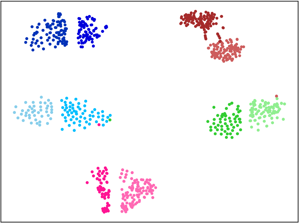
Figure 6: Embedding spaces learned by (left) parametric model [120], and (right) our nonparametric model. For better visualization, we show five classes of Cityscapes [23] with two prototypes per class.

C.5 Additional Qualitative Result

We show more qualitative results on ADE20K [142] (Fig. 7), Cityscapes [23] (Fig. 8) and COCO-Stuff [10] (Fig. 9). As observed, our approach generally gives more accurate predictions than SegFormer [120].

Appendix D Discussion

Limitation Analysis. One limitation of our approach is that it needs a clustering procedure during training, which increases the time complexity. However, in practice, the clustering algorithm imposes a minor computational burden, only taking about 2.5 ms to cluster 10K pixels into 10 prototypes. Additionally, like many other semantic segmentation models, our approach is subject to some factors such as domain gaps, label quality and fairness. We will put more efforts on improving the “in the wild” robustness of our model in the future research.

Broader Impact. This work provides a prototype perspective to unify existing mask decoding strategies, and accordingly introduces a novel non-learnable prototype based nonparametric segmentation scheme. On the positive side, the approach pushes the boundary of segmentation algorithms in terms of model efficiency and accuracy, and shows great potentials in unrestricted segmentation scenarios with thousands of semantic categories. Thus, the research could find diverse real-world applications such as self-driving cars and robot navigation. On the negative side, our model can be misused to segment the minority groups for malicious purposes. In addition, the problematic segmentation may cause inaccurate decision or planning of systems based on the results.

Future Work. This work also comes with new challenges, certainly worth further exploration:

• Closer Ties to Unsupervised Representation Learning. Our segmentation model directly learns the pixel embedding space with non-learnable prototypes. A critical success factor of recent unsupervised representation learning methods lies on the direct comparison of embeddings. By sharing such regime, our nonparametric model has good potential to make full use of unsupervised representations.

• Further Enhancing Interpretability. Our model only uses the mean of several embedded ‘support’ pixel samples as the prototype for each (sub-)class. To pursue better interpretability, one can optimize the prototypes to directly resemble actual pixels, or region-level observations [66, 53].

• Unifying Image-Wise and Pixel-Wise Classification. A common practice of building segmentation models is to remove the classification head from a pretrained classifier and leave the encoder. This is not optimal as lots of ‘knowledge’ are directly dropped. However, with prototype learning, one can transfer the ‘knowledge’ of a nonparametric classier to a nonparametric segmenter intactly, and formulate image-wise and pixel-wise classification in a unified paradigm.

Figure 7: Qualitative results of Segformer [120] and our approach on ADE20K [142] val.

Figure 8: Qualitative results of Segformer [120] and our approach on Cityscapes [23] val.

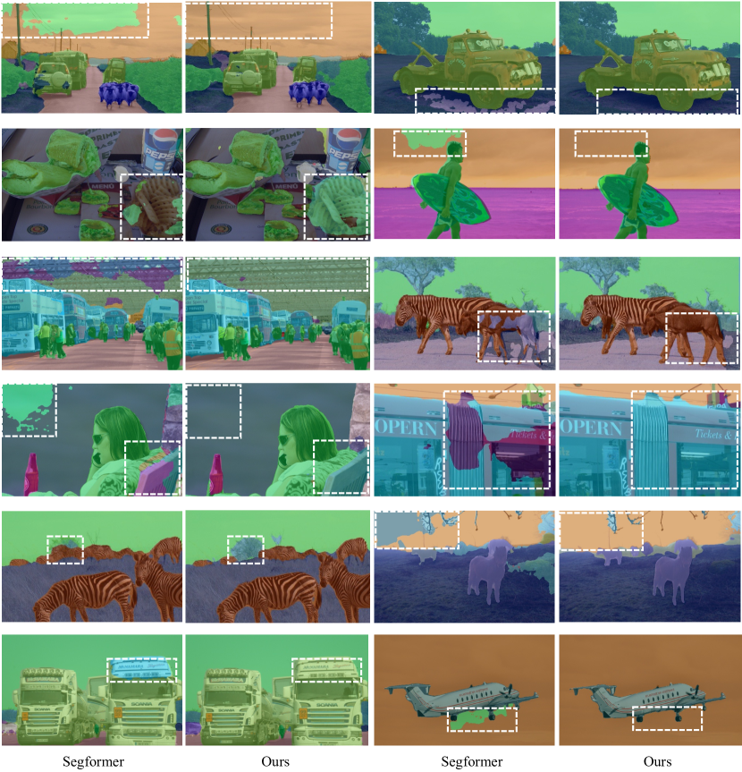
Figure 9: Qualitative results of Segformer [120] and our approach on COCO-Stuff [10] test.

References

- [1] Agnar Aamodt and Enric Plaza. Case-based reasoning: Foundational issues, methodological variations, and system approaches. AI Communications, 7(1):39–59, 1994.
- [2] Yuki Markus Asano, Christian Rupprecht, and Andrea Vedaldi. Self-labelling via simultaneous clustering and representation learning. In ICLR, 2020.
- [3] Andreas Backhaus and Udo Seiffert. Classification in high-dimensional spectral data: Accuracy vs. interpretability vs. model size. Neurocomputing, 131:15–22, 2014.
- [4] Vijay Badrinarayanan, Alex Kendall, and Roberto Cipolla. Segnet: A deep convolutional encoder-decoder architecture for image segmentation. IEEE TPAMI, 39(12):2481–2495, 2017.
- [5] Miguel A Bautista, Artsiom Sanakoyeu, Ekaterina Tikhoncheva, and Björn Ommer. Cliquecnn: Deep unsupervised exemplar learning. In NeurIPS, 2016.
- [6] Gedas Bertasius, Jianbo Shi, and Lorenzo Torresani. Semantic segmentation with boundary neural fields. In CVPR, 2016.
- [7] Michael Biehl, Barbara Hammer, Petra Schneider, and Thomas Villmann. Metric learning for prototype-based classification. In Innovations in Neural Information Paradigms and Applications, pages 183–199. 2009.
- [8] Michael Biehl, Barbara Hammer, and Thomas Villmann. Distance measures for prototype based classification. In International Workshop on Brain-Inspired Computing, 2013.
- [9] Christopher M Bishop. Pattern recognition. Machine learning, 128(9), 2006.
- [10] Holger Caesar, Jasper Uijlings, and Vittorio Ferrari. Coco-stuff: Thing and stuff classes in context. In CVPR, 2018.
- [11] Nicolas Carion, Francisco Massa, Gabriel Synnaeve, Nicolas Usunier, Alexander Kirillov, and Sergey Zagoruyko. End-to-end object detection with transformers. In ECCV, 2020.
- [12] Mathilde Caron, Piotr Bojanowski, Armand Joulin, and Matthijs Douze. Deep clustering for unsupervised learning of visual features. In ECCV, 2018.
- [13] Mathilde Caron, Ishan Misra, Julien Mairal, Priya Goyal, Piotr Bojanowski, and Armand Joulin. Unsupervised learning of visual features by contrasting cluster assignments. In NeurIPS, 2020.
- [14] Liang-Chieh Chen, Jonathan T Barron, George Papandreou, Kevin Murphy, and Alan L Yuille. Semantic image segmentation with task-specific edge detection using cnns and a discriminatively trained domain transform. In CVPR, 2016.
- [15] Liang-Chieh Chen, George Papandreou, Iasonas Kokkinos, Kevin Murphy, and Alan L Yuille. Deeplab: Semantic image segmentation with deep convolutional nets, atrous convolution, and fully connected crfs. IEEE TPAMI, 40(4):834–848, 2017.
- [16] Liang-Chieh Chen, Yukun Zhu, George Papandreou, Florian Schroff, and Hartwig Adam. Encoder-decoder with atrous separable convolution for semantic image segmentation. In ECCV, 2018.
- [17] Ting Chen, Simon Kornblith, Mohammad Norouzi, and Geoffrey Hinton. A simple framework for contrastive learning of visual representations. In ICML, 2020.
- [18] Wuyang Chen, Xinyu Gong, Xianming Liu, Qian Zhang, Yuan Li, and Zhangyang Wang. Fasterseg: Searching for faster real-time semantic segmentation. In ICLR, 2019.
- [19] Xinlei Chen, Haoqi Fan, Ross Girshick, and Kaiming He. Improved baselines with momentum contrastive learning. arXiv preprint arXiv:2003.04297, 2020.
- [20] Bowen Cheng, Alexander G. Schwing, and Alexander Kirillov. Per-pixel classification is not all you need for semantic segmentation. In NeurIPS, 2021.
- [21] Sungha Choi, Joanne T Kim, and Jaegul Choo. Cars can’t fly up in the sky: Improving urban-scene segmentation via height-driven attention networks. In CVPR, 2020.
- [22] MMSegmentation Contributors. MMSegmentation: Openmmlab semantic segmentation toolbox and benchmark. https://github.com/open-mmlab/mmsegmentation, 2020.
- [23] Marius Cordts, Mohamed Omran, Sebastian Ramos, Timo Rehfeld, Markus Enzweiler, Rodrigo Benenson, Uwe Franke, Stefan Roth, and Bernt Schiele. The cityscapes dataset for semantic urban scene understanding. In CVPR, 2016.
- [24] Thomas Cover and Peter Hart. Nearest neighbor pattern classification. IEEE TIT, 13(1):21–27, 1967.
- [25] Marco Cuturi. Sinkhorn distances: Lightspeed computation of optimal transport. In NeurIPS, 2013.
- [26] Jifeng Dai, Haozhi Qi, Yuwen Xiong, Yi Li, Guodong Zhang, Han Hu, and Yichen Wei. Deformable convolutional networks. In CVPR, 2017.
- [27] Bert De Brabandere, Davy Neven, and Luc Van Gool. Semantic instance segmentation for autonomous driving. In CVPR Workshop, 2017.
- [28] Henghui Ding, Xudong Jiang, Ai Qun Liu, Nadia Magnenat Thalmann, and Gang Wang. Boundary-aware feature propagation for scene segmentation. In CVPR, 2019.
- [29] Henghui Ding, Xudong Jiang, Bing Shuai, Ai Qun Liu, and Gang Wang. Semantic correlation promoted shape-variant context for segmentation. In CVPR, 2019.
- [30] Nanqing Dong and Eric P Xing. Few-shot semantic segmentation with prototype learning. In BMVC, 2018.
- [31] Alexey Dosovitskiy, Lucas Beyer, Alexander Kolesnikov, Dirk Weissenborn, Xiaohua Zhai, Thomas Unterthiner, Mostafa Dehghani, Matthias Minderer, Georg Heigold, Sylvain Gelly, et al. An image is worth 16x16 words: Transformers for image recognition at scale. In ICLR, 2020.
- [32] Richard O Duda, Peter E Hart, et al. Pattern classification and scene analysis, volume 3. Wiley New York, 1973.
- [33] David Eigen and Rob Fergus. Nonparametric image parsing using adaptive neighbor sets. In CVPR, 2012.
- [34] Jerome H Friedman. The elements of statistical learning: Data mining, inference, and prediction. Springer, 2009.
- [35] Jun Fu, Jing Liu, Haijie Tian, Yong Li, Yongjun Bao, Zhiwei Fang, and Hanqing Lu. Dual attention network for scene segmentation. In CVPR, 2019.
- [36] Jun Fu, Jing Liu, Yuhang Wang, Yong Li, Yongjun Bao, Jinhui Tang, and Hanqing Lu. Adaptive context network for scene parsing. In ICCV, 2019.
- [37] Salvador Garcia, Joaquin Derrac, Jose Cano, and Francisco Herrera. Prototype selection for nearest neighbor classification: Taxonomy and empirical study. IEEE TPAMI, 34(3):417–435, 2012.
- [38] Jacob Goldberger, Geoffrey E Hinton, Sam Roweis, and Russ R Salakhutdinov. Neighbourhood components analysis. In NeurIPS, 2004.
- [39] Samantha Guerriero, Barbara Caputo, and Thomas Mensink. Deepncm: Deep nearest class mean classifiers. In ICLR workshop, 2018.
- [40] Michael Gutmann and Aapo Hyvärinen. Noise-contrastive estimation: A new estimation principle for unnormalized statistical models. In AISTATS, 2010.
- [41] Raia Hadsell, Sumit Chopra, and Yann LeCun. Dimensionality reduction by learning an invariant mapping. In CVPR, 2006.
- [42] Adam W Harley, Konstantinos G Derpanis, and Iasonas Kokkinos. Segmentation-aware convolutional networks using local attention masks. In ICCV, 2017.
- [43] Junjun He, Zhongying Deng, and Yu Qiao. Dynamic multi-scale filters for semantic segmentation. In ICCV, 2019.
- [44] Junjun He, Zhongying Deng, Lei Zhou, Yali Wang, and Yu Qiao. Adaptive pyramid context network for semantic segmentation. In CVPR, 2019.
- [45] Kaiming He, Haoqi Fan, Yuxin Wu, Saining Xie, and Ross Girshick. Momentum contrast for unsupervised visual representation learning. In CVPR, 2020.
- [46] Kaiming He, Xiangyu Zhang, Shaoqing Ren, and Jian Sun. Deep residual learning for image recognition. In CVPR, 2016.
- [47] R Devon Hjelm, Alex Fedorov, Samuel Lavoie-Marchildon, Karan Grewal, Phil Bachman, Adam Trischler, and Yoshua Bengio. Learning deep representations by mutual information estimation and maximization. In ICLR, 2019.
- [48] Chi-Wei Hsiao, Cheng Sun, Hwann-Tzong Chen, and Min Sun. Specialize and fuse: Pyramidal output representation for semantic segmentation. In ICCV, 2021.
- [49] Hanzhe Hu, Deyi Ji, Weihao Gan, Shuai Bai, Wei Wu, and Junjie Yan. Class-wise dynamic graph convolution for semantic segmentation. In ECCV, 2020.
- [50] Jie Hu, Li Shen, and Gang Sun. Squeeze-and-excitation networks. In CVPR, 2018.
- [51] Zilong Huang, Xinggang Wang, Lichao Huang, Chang Huang, Yunchao Wei, and Wenyu Liu. Ccnet: Criss-cross attention for semantic segmentation. In ICCV, 2019.
- [52] Peter J Huber. Robust regression: asymptotics, conjectures and monte carlo. The annals of statistics, pages 799–821, 1973.
- [53] Jyh-Jing Hwang, Stella X Yu, Jianbo Shi, Maxwell D Collins, Tien-Ju Yang, Xiao Zhang, and Liang-Chieh Chen. Segsort: Segmentation by discriminative sorting of segments. In ICCV, 2019.
- [54] Shipra Jain, Danda Pani Paudel, Martin Danelljan, and Luc Van Gool. Scaling semantic segmentation beyond 1k classes on a single gpu. In ICCV, 2021.
- [55] Saumya Jetley, Bernardino Romera-Paredes, Sadeep Jayasumana, and Philip Torr. Prototypical priors: From improving classification to zero-shot learning. arXiv preprint arXiv:1512.01192, 2015.
- [56] Xu Ji, Joao F Henriques, and Andrea Vedaldi. Invariant information clustering for unsupervised image classification and segmentation. In ICCV, 2019.
- [57] Zhenchao Jin, Tao Gong, Dongdong Yu, Qi Chu, Jian Wang, Changhu Wang, and Jie Shao. Mining contextual information beyond image for semantic segmentation. In ICCV, 2021.
- [58] Zhenchao Jin, Bin Liu, Qi Chu, and Nenghai Yu. Isnet: Integrate image-level and semantic-level context for semantic segmentation. In ICCV, 2021.
- [59] Mahmut Kaya and Hasan Şakir Bilge. Deep metric learning: A survey. Symmetry, 11(9):1066, 2019.
- [60] Tsung-Wei Ke, Jyh-Jing Hwang, Ziwei Liu, and Stella X Yu. Adaptive affinity fields for semantic segmentation. In ECCV, 2018.
- [61] Barbara J Knowlton and Larry R Squire. The learning of categories: Parallel brain systems for item memory and category knowledge. Science, 262(5140):1747–1749, 1993.
- [62] Teuvo Kohonen. The self-organizing map. Neurocomputing, 21(1-3):1–6, 1998.
- [63] Shu Kong and Charless C Fowlkes. Recurrent pixel embedding for instance grouping. In CVPR, 2018.
- [64] Hanchao Li, Pengfei Xiong, Jie An, and Lingxue Wang. Pyramid attention network for semantic segmentation. arXiv preprint arXiv:1805.10180, 2018.
- [65] Junnan Li, Pan Zhou, Caiming Xiong, and Steven CH Hoi. Prototypical contrastive learning of unsupervised representations. In ICLR, 2020.
- [66] Oscar Li, Hao Liu, Chaofan Chen, and Cynthia Rudin. Deep learning for case-based reasoning through prototypes: A neural network that explains its predictions. In AAAI, 2018.
- [67] Xiangtai Li, Xia Li, Li Zhang, Guangliang Cheng, Jianping Shi, Zhouchen Lin, Shaohua Tan, and Yunhai Tong. Improving semantic segmentation via decoupled body and edge supervision. In ECCV, 2020.
- [68] Xia Li, Yibo Yang, Qijie Zhao, Tiancheng Shen, Zhouchen Lin, and Hong Liu. Spatial pyramid based graph reasoning for semantic segmentation. In CVPR, 2020.
- [69] Xia Li, Zhisheng Zhong, Jianlong Wu, Yibo Yang, Zhouchen Lin, and Hong Liu. Expectation-maximization attention networks for semantic segmentation. In ICCV, 2019.
- [70] Yanwei Li, Lin Song, Yukang Chen, Zeming Li, Xiangyu Zhang, Xingang Wang, and Jian Sun. Learning dynamic routing for semantic segmentation. In CVPR, 2020.
- [71] Guosheng Lin, Anton Milan, Chunhua Shen, and Ian Reid. Refinenet: Multi-path refinement networks for high-resolution semantic segmentation. In CVPR, 2017.
- [72] Tsung-Yi Lin, Michael Maire, Serge Belongie, James Hays, Pietro Perona, Deva Ramanan, Piotr Dollár, and C Lawrence Zitnick. Microsoft coco: Common objects in context. In ECCV, 2014.
- [73] Chenxi Liu, Liang-Chieh Chen, Florian Schroff, Hartwig Adam, Wei Hua, Alan L Yuille, and Li Fei-Fei. Auto-deeplab: Hierarchical neural architecture search for semantic image segmentation. In CVPR, 2019.
- [74] Ce Liu, Jenny Yuen, and Antonio Torralba. Sift flow: Dense correspondence across scenes and its applications. IEEE TPAMI, 33(5):978–994, 2010.
- [75] Ce Liu, Jenny Yuen, and Antonio Torralba. Nonparametric scene parsing via label transfer. IEEE TPAMI, 33(12):2368–2382, 2011.
- [76] Mingyuan Liu, Dan Schonfeld, and Wei Tang. Exploit visual dependency relations for semantic segmentation. In CVPR, 2021.
- [77] Weiyang Liu, Yandong Wen, Zhiding Yu, and Meng Yang. Large-margin softmax loss for convolutional neural networks. In ICML, 2016.
- [78] Ziwei Liu, Xiaoxiao Li, Ping Luo, Chen Change Loy, and Xiaoou Tang. Deep learning markov random field for semantic segmentation. IEEE TPAMI, 40(8):1814–1828, 2017.
- [79] Ze Liu, Yutong Lin, Yue Cao, Han Hu, Yixuan Wei, Zheng Zhang, Stephen Lin, and Baining Guo. Swin transformer: Hierarchical vision transformer using shifted windows. In ICCV, 2021.
- [80] Jonathan Long, Evan Shelhamer, and Trevor Darrell. Fully convolutional networks for semantic segmentation. In CVPR, 2015.
- [81] Tomasz Malisiewicz and Alexei A Efros. Recognition by association via learning per-exemplar distances. In CVPR, 2008.
- [82] Sachin Mehta, Mohammad Rastegari, Anat Caspi, Linda Shapiro, and Hannaneh Hajishirzi. Espnet: Efficient spatial pyramid of dilated convolutions for semantic segmentation. In ECCV, 2018.
- [83] Tim Meinhardt, Alexander Kirillov, Laura Leal-Taixe, and Christoph Feichtenhofer. Trackformer: Multi-object tracking with transformers. arXiv preprint arXiv:2101.02702, 2021.
- [84] Pascal Mettes, Elise van der Pol, and Cees Snoek. Hyperspherical prototype networks. In NeurIPS, 2019.
- [85] Tom M Mitchell. The need for biases in learning generalizations. Department of Computer Science, Laboratory for Computer Science Research, 1980.
- [86] Vladimir Nekrasov, Hao Chen, Chunhua Shen, and Ian Reid. Fast neural architecture search of compact semantic segmentation models via auxiliary cells. In CVPR, 2019.
- [87] Davy Neven, Bert De Brabandere, Marc Proesmans, and Luc Van Gool. Instance segmentation by jointly optimizing spatial embeddings and clustering bandwidth. In CVPR, 2019.
- [88] Allen Newell, Herbert Alexander Simon, et al. Human problem solving, volume 104. 1972.
- [89] Aaron van den Oord, Yazhe Li, and Oriol Vinyals. Representation learning with contrastive predictive coding. arXiv preprint arXiv:1807.03748, 2018.
- [90] Tianyu Pang, Kun Xu, Yinpeng Dong, Chao Du, Ning Chen, and Jun Zhu. Rethinking softmax cross-entropy loss for adversarial robustness. In ICLR, 2020.
- [91] Olaf Ronneberger, Philipp Fischer, and Thomas Brox. U-net: Convolutional networks for biomedical image segmentation. In MICCAI, 2015.
- [92] Eleanor H Rosch. Natural categories. Cognitive psychology, 4(3):328–350, 1973.
- [93] Olga Russakovsky, Jia Deng, Hao Su, Jonathan Krause, Sanjeev Satheesh, Sean Ma, Zhiheng Huang, Andrej Karpathy, Aditya Khosla, Michael S. Bernstein, Alexander C. Berg, and Fei-Fei Li. Imagenet large scale visual recognition challenge. IJCV, 115(3):211–252, 2015.
- [94] Ruslan Salakhutdinov and Geoff Hinton. Learning a nonlinear embedding by preserving class neighbourhood structure. In Artificial Intelligence and Statistics, pages 412–419, 2007.
- [95] Mark Sandler, Andrew Howard, Menglong Zhu, Andrey Zhmoginov, and Liang-Chieh Chen. Mobilenetv2: Inverted residuals and linear bottlenecks. In CVPR, 2018.
- [96] Atsushi Sato and Keiji Yamada. Generalized learning vector quantization. In NeurIPS, 1995.
- [97] Florian Schroff, Dmitry Kalenichenko, and James Philbin. Facenet: A unified embedding for face recognition and clustering. In CVPR, 2015.
- [98] John Shawe-Taylor, Nello Cristianini, et al. Kernel methods for pattern analysis. Cambridge university press, 2004.
- [99] Karen Simonyan and Andrew Zisserman. Very deep convolutional networks for large-scale image recognition. In ICLR, 2015.
- [100] Jake Snell, Kevin Swersky, and Richard S Zemel. Prototypical networks for few-shot learning. In NeurIPS, 2017.
- [101] Kihyuk Sohn. Improved deep metric learning with multi-class n-pair loss objective. In NeurIPS, 2016.
- [102] Robin Strudel, Ricardo Garcia, Ivan Laptev, and Cordelia Schmid. Segmenter: Transformer for semantic segmentation. In ICCV, 2021.
- [103] Guolei Sun, Wenguan Wang, Jifeng Dai, and Luc Van Gool. Mining cross-image semantics for weakly supervised semantic segmentation. In ECCV, 2020.
- [104] Joseph Tighe and Svetlana Lazebnik. Superparsing: scalable nonparametric image parsing with superpixels. In ECCV, 2010.
- [105] Antonio Torralba, Rob Fergus, and William T Freeman. 80 million tiny images: A large data set for nonparametric object and scene recognition. IEEE TPAMI, 30(11):1958–1970, 2008.
- [106] Wouter Van Gansbeke, Simon Vandenhende, Stamatios Georgoulis, Marc Proesmans, and Luc Van Gool. Scan: Learning to classify images without labels. In ECCV, 2020.
- [107] Ashish Vaswani, Noam Shazeer, Niki Parmar, Jakob Uszkoreit, Llion Jones, Aidan N Gomez, Lukasz Kaiser, and Illia Polosukhin. Attention is all you need. In NeurIPS, 2017.
- [108] Oriol Vinyals, Charles Blundell, Timothy Lillicrap, Daan Wierstra, et al. Matching networks for one shot learning. In NeurIPS, 2016.
- [109] Jiang Wang, Yang Song, Thomas Leung, Chuck Rosenberg, Jingbin Wang, James Philbin, Bo Chen, and Ying Wu. Learning fine-grained image similarity with deep ranking. In CVPR, 2014.
- [110] Jingdong Wang, Ke Sun, Tianheng Cheng, Borui Jiang, Chaorui Deng, Yang Zhao, Dong Liu, Yadong Mu, Mingkui Tan, Xinggang Wang, et al. Deep high-resolution representation learning for visual recognition. IEEE TPAMI, 2020.
- [111] Kaixin Wang, Jun Hao Liew, Yingtian Zou, Daquan Zhou, and Jiashi Feng. Panet: Few-shot image semantic segmentation with prototype alignment. In ICCV, 2019.
- [112] Wenguan Wang, Tianfei Zhou, Siyuan Qi, Jianbing Shen, and Song-Chun Zhu. Hierarchical human semantic parsing with comprehensive part-relation modeling. IEEE TPAMI, 2021.
- [113] Wenguan Wang, Tianfei Zhou, Fisher Yu, Jifeng Dai, Ender Konukoglu, and Luc Van Gool. Exploring cross-image pixel contrast for semantic segmentation. In ICCV, 2021.
- [114] Xiaolong Wang, Ross Girshick, Abhinav Gupta, and Kaiming He. Non-local neural networks. In CVPR, 2018.
- [115] Yuqing Wang, Zhaoliang Xu, Xinlong Wang, Chunhua Shen, Baoshan Cheng, Hao Shen, and Huaxia Xia. End-to-end video instance segmentation with transformers. In CVPR, 2021.
- [116] Yandong Wen, Kaipeng Zhang, Zhifeng Li, and Yu Qiao. A discriminative feature learning approach for deep face recognition. In ECCV, 2016.
- [117] Zhirong Wu, Alexei A Efros, and Stella X Yu. Improving generalization via scalable neighborhood component analysis. In ECCV, 2018.
- [118] Zhirong Wu, Yuanjun Xiong, Stella X Yu, and Dahua Lin. Unsupervised feature learning via non-parametric instance discrimination. In CVPR, 2018.
- [119] Tete Xiao, Yingcheng Liu, Bolei Zhou, Yuning Jiang, and Jian Sun. Unified perceptual parsing for scene understanding. In ECCV, 2018.
- [120] Enze Xie, Wenhai Wang, Zhiding Yu, Anima Anandkumar, Jose M Alvarez, and Ping Luo. Segformer: Simple and efficient design for semantic segmentation with transformers. In NeurIPS, 2021.
- [121] Junyuan Xie, Ross Girshick, and Ali Farhadi. Unsupervised deep embedding for clustering analysis. In ICML, 2016.
- [122] Wenjia Xu, Yongqin Xian, Jiuniu Wang, Bernt Schiele, and Zeynep Akata. Attribute prototype network for zero-shot learning. In NeurIPS, 2020.
- [123] Kouta Nakata Yaling Tao, Kentaro Takagi. Clustering-friendly representation learning via instance discrimination and feature decorrelation. In ICLR, 2021.
- [124] Xueting Yan, Ishan Misra, Abhinav Gupta, Deepti Ghadiyaram, and Dhruv Mahajan. Clusterfit: Improving generalization of visual representations. In CVPR, 2020.
- [125] Hong-Ming Yang, Xu-Yao Zhang, Fei Yin, and Cheng-Lin Liu. Robust classification with convolutional prototype learning. In CVPR, 2018.
- [126] Maoke Yang, Kun Yu, Chi Zhang, Zhiwei Li, and Kuiyuan Yang. Denseaspp for semantic segmentation in street scenes. In CVPR, 2018.
- [127] Yi Yang, Yueting Zhuang, and Yunhe Pan. Multiple knowledge representation for big data artificial intelligence: framework, applications, and case studies. Frontiers of Information Technology & Electronic Engineering, 22(12):1551–1558, 2021.
- [128] Changqian Yu, Jingbo Wang, Changxin Gao, Gang Yu, Chunhua Shen, and Nong Sang. Context prior for scene segmentation. In CVPR, 2020.
- [129] Changqian Yu, Jingbo Wang, Chao Peng, Changxin Gao, Gang Yu, and Nong Sang. Learning a discriminative feature network for semantic segmentation. In CVPR, 2018.
- [130] Fisher Yu and Vladlen Koltun. Multi-scale context aggregation by dilated convolutions. In ICLR, 2016.
- [131] Yuhui Yuan, Xilin Chen, and Jingdong Wang. Object-contextual representations for semantic segmentation. In ECCV, 2020.
- [132] Yuhui Yuan, Rao Fu, Lang Huang, Weihong Lin, Chao Zhang, Xilin Chen, and Jingdong Wang. Hrformer: High-resolution transformer for dense prediction. In NeurIPS, 2021.
- [133] Yuhui Yuan, Jingyi Xie, Xilin Chen, and Jingdong Wang. Segfix: Model-agnostic boundary refinement for segmentation. In ECCV, 2020.
- [134] Hang Zhang, Kristin Dana, Jianping Shi, Zhongyue Zhang, Xiaogang Wang, Ambrish Tyagi, and Amit Agrawal. Context encoding for semantic segmentation. In CVPR, 2018.
- [135] Kai Zhang, James T Kwok, and Bahram Parvin. Prototype vector machine for large scale semi-supervised learning. In ICML, 2009.
- [136] Xiao Zhang, Rui Zhao, Yu Qiao, and Hongsheng Li. Rbf-softmax: Learning deep representative prototypes with radial basis function softmax. In ECCV, 2020.
- [137] Hengshuang Zhao, Jianping Shi, Xiaojuan Qi, Xiaogang Wang, and Jiaya Jia. Pyramid scene parsing network. In CVPR, 2017.
- [138] Hengshuang Zhao, Yi Zhang, Shu Liu, Jianping Shi, Chen Change Loy, Dahua Lin, and Jiaya Jia. Psanet: Point-wise spatial attention network for scene parsing. In ECCV, 2018.
- [139] Mingmin Zhen, Jinglu Wang, Lei Zhou, Shiwei Li, Tianwei Shen, Jiaxiang Shang, Tian Fang, and Long Quan. Joint semantic segmentation and boundary detection using iterative pyramid contexts. In CVPR, 2020.
- [140] Shuai Zheng, Sadeep Jayasumana, Bernardino Romera-Paredes, Vibhav Vineet, Zhizhong Su, Dalong Du, Chang Huang, and Philip HS Torr. Conditional random fields as recurrent neural networks. In ICCV, 2015.
- [141] Sixiao Zheng, Jiachen Lu, Hengshuang Zhao, Xiatian Zhu, Zekun Luo, Yabiao Wang, Yanwei Fu, Jianfeng Feng, Tao Xiang, Philip HS Torr, et al. Rethinking semantic segmentation from a sequence-to-sequence perspective with transformers. In CVPR, 2021.
- [142] Bolei Zhou, Hang Zhao, Xavier Puig, Sanja Fidler, Adela Barriuso, and Antonio Torralba. Scene parsing through ade20k dataset. In CVPR, 2017.
- [143] Tianfei Zhou, Liulei Li, Xueyi Li, Chun-Mei Feng, Jianwu Li, and Ling Shao. Group-wise learning for weakly supervised semantic segmentation. IEEE TIP, 31:799–811, 2021.