DeepShadow: Neural Shape from Shadow

Abstract

This paper presents ‘DeepShadow’, a one-shot method for recovering the depth map and surface normals from photometric stereo shadow maps. Previous works that try to recover the surface normals from photometric stereo images treat cast shadows as a disturbance. We show that the self and cast shadows not only do not disturb 3D reconstruction, but can be used alone, as a strong learning signal, to recover the depth map and surface normals. We demonstrate that 3D reconstruction from shadows can even outperform shape-from-shading in certain cases. To the best of our knowledge, our method is the first to reconstruct 3D shape-from-shadows using neural networks. The method does not require any pre-training or expensive labeled data, and is optimized during inference time.

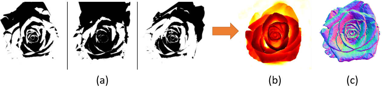
Figure 1: Results on the rose object. (a) Input shadow maps, which were used for supervision (b) Depth produced by the algorithm. (c) Surface normals extracted from the depth map.

1 Introduction

The photometric stereo setting was first defined in [29]. The setting includes a single camera viewpoint, and multiple varying illumination sources. Most works try to extract the underlying per-pixel normal map from the input images. The original problem assumed Lambertian objects, which only have a diffuse reflectance component. More recent works solve a more general setting, with various light and material properties, including specular components.

To date, most works extract the required information from the local illumination effect, defined by the bidirectional reflectance distribution function (BRDF), and either ignored the global cast shadow effect, or model it in a statistical way. Almost all recent works use Conv Nets to recover the 3D structure from photometric stereo. Since Conv Nets have limited receptive fields, global information can only be aggregated in the deeper layers where accurate spatial resolution is limited.

In our work, we extract the depth information directly from the cast shadows. As far as we know, this is the first attempt to do so using neural networks. In the photometric stereo setting, cast and attached shadow detection is a relatively easy learning task. The shadow maps are binary inputs, i.e., have a 0 or 1 value. To extract depth, we initially predict per-pixel depth information in 2D and thereafter produce a point-cloud in 3D from this prediction. The 3D points are then used to calculate global cast shadows, by tracing the light source to all destination pixels. The input images are used as supervision for the produced shadow maps. The entire process is differentiable, and the predicted depth can be learned using optimization. Our process is physics based and can aggregate global information while keeping the full resolution of the image.

Most previous works assume directional lights due to its simplicity, although this is usually not the case. Many scenes consist of point light sources, thus depth information should be extracted using a point light shading model. In this work, we assume images generated by point light sources, but we can easily extend our method to handle directional lights. Although the inputs in this work are only shadow maps, our method can be integrated with existing shape-from-shading models, in order to improve their results in complex shadowed scenes. Our code and data are available at https://asafkar.github.io/deepshadow/.

2 Related Work

Shape Reconstruction from Shadows Extracting shape information from shadows has been attempted in various works. This was mostly done before the deep learning era. An early attempt was performed in [9], which initializes a shadow map and sets lower and upper bounds on expected illuminated or shadowed pixels, which are then optimized until reaching a predicted height map. In [32], a graph-based representation is used to incorporate constraints induced by the shadow maps. This work also optimizes the height map using iteration based on low and high bounds. The ShadowCuts [2] work performs Lambertian photometric stereo with shadows present. It initially uses a graph-cut method for estimating light source visibility for every pixel. Then it uses the produced shadow maps along with shading information to perform surface normal integration, to produce the final predicted surface. In [30], the authors use 1D shadow graphs to speed up the 3D reconstruction process. 1D slices (i.e., rows or columns of the shadow images) are used, assuming the light source moves in two independent circular orbits. Each such slice can be solved independently, to retrieve the corresponding 1D slice of the underlying height map. This method only handles light sources that are on a unit sphere, and the trajectories of the light sources must be perpendicular to each other. All the above works extract the shadow maps from the images using a hand-picked threshold. A recent method [19] uses an initial approximation of the 3D geometry as input to optimize object deformations by using soft shadow information. In contrary, our method does not require an initial approximation of the geometry. The method uses spherical harmonics to approximate the surface occlusion whereas we use implicit representations along with a linear-time tracing method.

Implicit Representations Implicit representations have recently been used to replace voxel grids or meshes with continues parameterization using neural networks. These are used in [20] to query the color and opacity of a certain point in space, to produce the pixel color of an image acquired from a specific viewing position. Lately, implicit representations have also been used in works such as [1, 27, 34] to recover various underlying geometric and photometric properties such as albedo, normals, etc. These have all been done in multi-view settings and take many hours and days to optimize.

Viewshed Analysis Viewshed analysis solves the problem of which areas are visible from a specific viewpoint, and solved in [7, 13] using a line-of-sight (LOS) algorithm. This algorithm tracks along a ray from the viewpoint to the target point, while verifying that the target point is not occluded by the height points along the ray. Shapira [25] proposed the R3 method for viewshed computation, by generating LOS rays from the viewpoint to all other cells (pixels) in a height map. Franklin et al. [12] introduced the R2 algorithm, which optimizes the R3 method by launching LOS rays only to the outer cells (boundary pixels), while computing and storing the intermediate results of all cells on the way. This method is considered an approximation since some rays will encounter the same cells during the process.

Photometric Stereo In the past few years, various learning-based methods have been proposed to solve calibrated and uncalibrated photometric stereo problems [15, 5, 4, 31, 18]. Most existing methods solve the problem in a supervised manner, i.e., given inputs of N images and their associated light directions and intensities, the methods predict the surface normals as an output. The ground-truth normals are needed as supervision in order to train the network. In the uncalibrated scenarios, the light intensities and directions are not required. Works such as [5, 6] first regress the light direction and light intensities, and then solve the calibrated photometric stereo problem using the predicted lights. Methods such as [15, 28] solve the problem in an unsupervised manner, using a reconstruction loss. These methods only require the input images, which are used as self-supervision in the reconstruction loss.

Most of the above-mentioned methods use the pixelwise information to solve the problem. No inter-pixel relations are taken into account, besides the obvious local dependencies resulting from the local filtering. There are also methods such as [31, 18] that use local neighborhood pixels as well by feature aggregation. In [31], the authors use a graph-based neural network to unify all-pixel and per-pixel information, while in [18] the authors use each pixel as a data-point to learn interactions between pixels. Although the latter method does handle cast shadows, it does so within a bound area of the observation map and in a statistical manner. Apart from this method, the previous methods ignore the cast shadows as a source of information, and treat them as a disturbance.

Some work solve the near-field photometric stereo problem, which assumes that the lights are close to the object, and thus cannot use directional lights. In [23], the authors use a hybrid approach that utilizes both distant and near-field models. The surface normals of a local area are computed by assuming they are illuminated by a distant light source, and the reconstruction error is based on the near field model. This method yields good results for close range lights, although it requires knowing the mean depth for initialization. It also requires the location of the point lights as well as the ambient lighting. The work in [17] also uses a far and near hybrid method, by first predicting the surface normals assuming far light sources, and then computing the depth by integrating the normal fields. The normal fields are then used to estimate light directions and attenuation that are used to compute the reflectance.

We also mention [22, 14], which produce high resolution depth maps by using low resolution depth maps and photometric stereo images. Since few photometric stereo-based methods target depth outputs, we will compare our work with [22].

In summary, most previous shape-from-shading methods need a large amount of data for training. Also, they ignore the cast shadow instead of using it as a source of information. The main contributions of our method are:

• We propose the first deep-learning based method for recovering depth and surface normals from shadow maps.

• Our method includes a shadow calculation component, which globally aggregates information in the spatial space.

• Our method uses linear-time calculation rather than quadratic complexity in [20] and its follow-up works. We also use 2D parameterization for depth maps, avoiding the expensive 3D parameterization in NeRF like works.

• In contrast to most shape-from-shading methods, which use photometric stereo data, our method is insensitive to non-diffuse reflectance (specular highlights) or varying intensity lights, which also enables it to generate good results in both from the near-field and far-light photometric stereo settings.

• Lastly, our method estimates the depth-map in a one-shot manner, avoiding costly data collection and supervised training.

3 Shape-from-Shadow Method

DeepShadow is a technique that estimates the shape of an object or a scene from cast and attached shadows. The input data are multiple shadow maps and the location of their associated point light sources. In our work, these can later be relaxed to input images alone. Similarly to photometric stereo, the data are generated or captured with a single viewpoint and multiple illuminations. We assume each input shadow map is a byproduct of a single image taken under a single light source. In contrast to other methods that use directional lights, we do not enforce the location of the point light to be on a unit sphere. Our algorithm can also work with directional light, which models a light source at infinity.

Figure 2 shows our framework. First, a multi-layer perceptron (MLP) predicts the depth at each given location $\mathbf{u}=(u,v)$ in the image. Positional encoding $\gamma(\mathbf{u})$ is used at the input of the MLP. Then, the predicted depth $\hat{d}$ along with an input light location $L^{j}$ are used to estimate a shadow map $\hat{S^{j}}$. This is a physics based component which is differentiable but not trainable. The associated ground-truth shadow map $S^{j}$ is used for supervision to optimize the MLP.

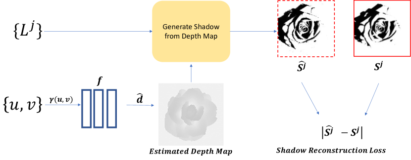
Figure 2: Algorithm Overview. DeepShadow takes the light source location $L^{j}$ and pixel coordinates $({u,v)}$ as inputs, along with the estimated depth $\hat{d}$ from the MLP, and outputs an estimate of the shadow map $\hat{S^{j}}$ at each pixel location. The ground-truth shadow map $S^{j}$ is then used as a supervision to optimize the learned depth map.

3.1 Shadow Map Estimation

To calculate the shadow of a pixel with respect to a specific light source $L^{j}$, the ‘shadow line scan’ algorithm is used. This algorithm traces a light ray from the light source to the destination pixel, and determines whether the pixel is illuminated or shadowed. More details are provided in Section 3.2.

To produce a shadow map from an estimated depth map, we use both world coordinates $\mathbf{X}=\{x,y,z\}$ and image coordinates $\mathbf{u}=\{u,v\}$ on the image plane. We assume the calibrated camera model is known. During the process, we use perspective projection and unprojection to go from one coordinate system to the other. Thus for a certain pixel location $\mathbf{u}_{i}$, $\mathbf{u}_{i}=P\mathbf{X}_{i}$, where $P$ is the projection matrix $P=K\cdot[R|\mathbf{t}]$, $K$ is the intrinsic matrix and $[R|\mathbf{t}]$ is the extrinsic matrix.

For a given light source $L^{j}=(L_{x}^{j},L_{y}^{j},L_{z}^{j})$ in world coordinates, we initially map the light source to a point $\boldsymbol{\ell}^{j}=P\cdot L^{j}$ on the image plane. To estimate the shadow for a chosen pixel $\mathbf{u}_{i}=(u_{i},v_{i})$ in the image, a line $\mathbf{r}_{i}^{j}$ of points in the image plane is generated between $\boldsymbol{\ell}^{j}$ and $\mathbf{u}_{i}$:

$$\mathbf{r}_{i}^{j}(\alpha)=(1-\alpha)\boldsymbol{\ell}^{j}+\alpha\mathbf{u}_{i},~{}~{}\alpha\in[0,1]$$ (1)

Points on $\mathbf{r}^{j}_{i}$ that are outside the image frame are excluded. For each pixel in $\mathbf{r}_{i}^{j}(\alpha)$, we estimate the depth $\hat{d}_{i}^{j}(\alpha)$ by querying the MLP model at the pixel’s coordinates. Each such triplet $(\mathbf{r}_{i}^{j}(\alpha)[x],\mathbf{r}_{i}^{j}(\alpha)[y],\hat{d}_{i}^{j}(\alpha))$ is then unprojected to world coordinates to receive its 3D location $R_{i}^{j}(\alpha)$ as described in Equation 2 and illustrated in Figure 3a.

$$R_{i}^{j}(\alpha)=P^{-1}\mathbf{r}_{i}^{j}(\alpha)\cdot\hat{d}_{i}^{j}(\alpha)~{},~{}\alpha\in[0,1]$$ (2)

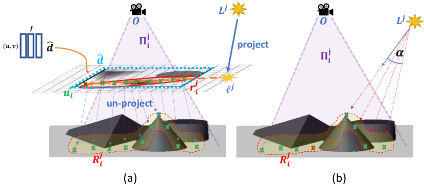
Figure 3: Flow of shape-from-shadow. (a) The light source $L^{j}$ is projected onto the image plane to receive $\boldsymbol{\ell}^{j}$. A ray $\mathbf{r}_{i}^{j}$ of $(u,v)$ points is created between $\boldsymbol{\ell}^{j}$ and $\mathbf{u}_{i}$. Then, each point with its estimated depth $\hat{d}$ is unprojected to world coordinates. (b) The shadow line scan algorithm is used on points in 3D space to calculate shadowed pixels. Red points are shadowed, since their angle to the light source is smaller than $\alpha$.

Once the 3D coordinates for each pixel in $R^{j}_{i}$ are obtained, we can solve this as a 1D line-of-sight problem, as illustrated in Figure 3b. Note, that this process will determine, for each point in $R^{j}_{i}$, whether it is shadowed or illuminated (and not only for the point $\mathbf{u}_{i}$). We use the image plane coordinates for parameterization of the depth, thus avoiding a costly full 3D parameterization (as in [20] and follow up works). This process assumes the object’s depth is a function of $(u,v)$, which is a justifiable assumption since we are solving for the case of a single viewpoint.

Note that the light source $L^{j}$, viewer location $O$ and a given point $\mathbf{u}_{i}$ create a plane $\Pi_{i}^{j}$ in 3D, as can be seen in Figure 3b. $\boldsymbol{\ell}^{j}$ is also located on $\Pi_{i}^{j}$, as are all the points in $\mathbf{r}_{i}^{j}$ and all the points in $R_{j}^{j}$. This enables us to use a 1D line-of-sight algorithm between $L^{j}$ and all points in $R_{i}^{j}$ (elaborated in Section 3.2).

We emphasize that the shadow calculation depends only on the locations of the light source and the depth map. The camera’s center of projection (COP) $O$ is used to generate the scan order for points along a 1D ray, and to expedite calculations as will be described in the next section.

3.2 Shadow Line Scan Algorithm

Given a height map and a viewer location, one can analyze all points visible to the viewer using a ‘line-of-sight’ calculation. This process identifies which areas are visible from a given point. It can be naively achieved by sending 1D rays to every direction from the viewer, and calculating the line-of-sight visibility for each ray. This is analogous to producing shade maps – the viewer is replaced with a light source $L^{j}$, and every pixel is analyzed to determine whether it is shadowed (visible from $L^{j}$) or not, in the same manner. We refer to this process as ‘shadow line scan’.

Calculating the visibility of each pixel point is time consuming and may take many hours to train. Instead, we propose to calculate the visibility of entire lines in the image. Each line $R^{j}_{i}$ is calculated using a single scan. Each line includes the projections of all the points in 3D that are in the plane $\Pi^{j}_{i}$ that is formed by the COP $O$, $L^{j}$ and $\mathbf{u}_{i}$.

As is illustrated in Figure 4, we define a vector from the light source $L^{j}$ to each point in $R^{j}_{i}$, as

$$V_{i}^{j}(\alpha)=L^{j}-R_{i}^{j}(a).$$ (3)

Since we use the shadow maps as supervision and the shadow maps are composed of discrete pixels, we use discrete alpha values $\alpha\rightarrow{}\{\alpha_{i}\}^{T}_{i=0}$. We calculate all the angles between $V_{i}^{j}[a_{0}]$ and each of the points. The angle for the $i^{th}$ point is defined as

$$ang[i]=\arccos{\left(\frac{V_{i}^{j}[\alpha_{0}]\cdot V_{i}^{j}[\alpha_{i}]}{\|V_{i}^{j}[\alpha_{0}]\|\cdot\|V_{i}^{j}[\alpha_{i}]\|+\epsilon}\right)}$$ (4)

For numerical stability, $\epsilon$ is added to the denominator. $ang[i]$ is then compared to all previous angles $\{ang[k]~{}\mid~{}k\leq i\}$. If the current angle is larger than all previous angles, the current point is visible from the light source location and thus has no shadow. Otherwise, the point (pixel) is shadowed. A visualization of the process can be seen in Fig. 4.

This process can be reduced to a cumulative maximum function as defined in Equation 5. To achieve the final shadow estimate in Equation 6 we use a Sigmoid function to keep the final values between 0 and 1.

$$s_{L}[\alpha_{i}]=\max\big{(}ang[\alpha_{i}],s_{L}[\alpha_{i-1}]\big{)}$$ (5)

$$s[\alpha_{i}]=2\sigma{\Big{(}ang[\alpha_{i}]-s_{L}[\alpha_{i}]\Big{)}}$$ (6)

The cumulative maximum function was chosen since it is differentiable, similar to the well-known ReLU function. The rest of the process is also differentiable, and can be used to learn the depth map similar to what is done in inverse rendering methods.

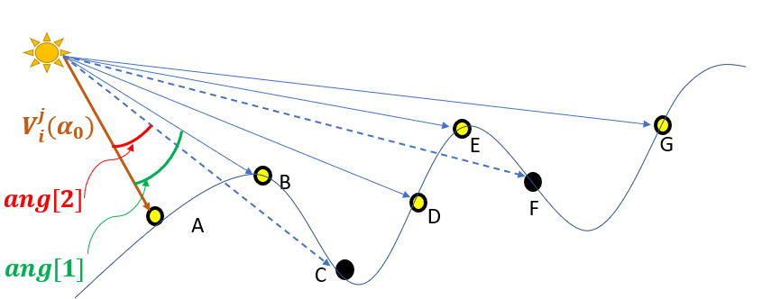
Figure 4: 1D Shadow Line Scan Algorithm for Shadow Calculation. Points A–B are visible to the viewer, thus have no shadows. The angle $ang[2]$ between A and C (red) is smaller than the angle $ang[1]$ between A and B (green), thus C is not visible. Similarly, the angle between A and F is smaller than the last encountered largest angle, A–E, making F shadowed as well.

3.3 Learning Depth from Shadows

For a given light source $L^{j}$, a dense estimated shadow map is produced by generating the shadow prediction for each pixel. The shadow line scan algorithm is applied for many lines in the image, covering the entire set of pixels, in order to generate a dense shadow map $\hat{S}^{j}$. The ground-truth shadow map can then be used for supervision, to learn the depth. Once finished, the optimized MLP can be used to generate a dense predicted depth map.

3.4 Computational Aspects

In [20] and similar follow-up works, to predict the pixel color, an integral must be calculated along a ray of samples. This requires quadratic computation complexity relative to the image size. In our work, the calculation takes linear time, since shadow predictions for all pixels along a shadow line scan can be calculated in a cumulative manner. The intermediate shadow results for a particular pixel and the maximum angle thus far are stored and used in the next pixel calculation along the line. We used the boundary sampling method (R2) [12], which sends LOS rays from the light source to the boundary of image only, instead of sending rays to all pixels. Although this method is considered less accurate than the R3 [25] method which calculates results for all pixels, it requiring an order of magnitude fewer calculations. The R2 method can also be sub-sampled using a coarse-to-fine sampling scheme. In the early iterations, rather than taking all pixels in the boundary, one can take every $k_{th}$ pixel. Since the light locations vary, we will most likely use all pixels in the depth map at least once.

3.5 Loss Function

We used a loss composed of the reconstruction loss and a depth-guided regularization loss. The general loss is:

$$\mathcal{L}=\frac{1}{N}\sum_{j}\mathcal{L}_{rec}^{j}+\lambda\mathcal{L}_{d}$$ (7)

where $\mathcal{L}_{rec}^{j}$ is the reconstruction loss:

$$\mathcal{L}_{rec}^{j}=\frac{1}{HW}|S^{j}-\hat{S^{j}}|.$$ (8)

$\mathcal{L}_{d}$ is a depth regularization term:

$$\mathcal{L}_{d}=\sum_{ij}\left|\partial_{x}\hat{d}_{ij}\right|e^{-\left\|\partial_{x}\overline{I}_{ij}\right\|}+\left|\partial_{y}\hat{d}_{ij}\right|e^{-\left\|\partial_{y}\overline{I}_{ij}\right\|},$$ (9)

where $\hat{d}_{ij}=\hat{d}(u_{i},v_{j})$ is the estimated depth at pixel $(u_{i},v_{j})$, $\partial_{x}$ and $\partial_{y}$ are gradients in the horizontal and vertical directions, and $\overline{I}$ is the average color over all input images. Similar to [33], we assume that the average image edges provide a signal for the object discontinuity. This regularization term helps the depth map to converge faster.

4 Experimental Results

We compare our method to several shape-from-shading methods. While these methods require illuminated images as input (and we only require binary shadow maps) we find that this comparison illustrates the complementary nature of our method to shape-from-shading. As we will show, results depend on the statistics of the input objects, and for several classes of objects we achieve superior results to shape-from-shading even though we use less data.

4.1 Implementation details

We represent the continuous 2D depth map as a function of $\mathbf{u}=(u,v)$. Similar to [20], we approximate this function with an MLP $F_{w}(\mathbf{u})=\hat{d}$. We used six-layer MLP with a latent dimension of 128, along with sine activation functions, similar to [26]. The MLP was initialized according to [26].

We implemented this using PyTorch [21]. We optimized the neural network using the Adam optimizer [16] with an initial learning rate of 5 x $10^{-5}$, which was decreased every 15 epochs by a factor of 0.9. We reduce the temperature of the Sigmoid function 3 times during the optimization process, using a specific schedule. We run the optimization until the loss plateaus, which typically takes an hour on an input of 16 images with spatial resolution of 256x256, using an Intel i9-10900X CPU and an NVIDIA GeForce RTX 2080 Ti. The current implementation uses a single-process and contains many occurrences of native Python indexing, thus is sub-optimal and can be further optimized.

Photometric-stereo data is not usually accompanied by labeled shadow masks. Thus, for datasets which have no ground-truth shadows or light directions, we implement a model to estimate these. We use the Blobby and Sculptures datasets from [3] along with our own shadow dataset in order to train the model. Details can be found in the supplementary material.

4.2 Datasets

We show results on nine synthetic objects: 3 from previous work [15] and 6 curated and rendered by us from Sketchfab. The objects we selected span various shapes and sizes, and they also possess one key property: many 3D features that cast shadows. As we will show, when this property holds, our method outperforms shape-from-shading methods and thus complements them. Our objects were each rendered with 16 different illumination conditions. Scenes are illuminated by a single point-light source.

Since shadow maps are not available in the dataset of Kaya et al. [15], we have our previously mentioned shadow-extraction model to estimate these. For our rendered objects, we use the ground-truth shadow maps as inputs. Qualitative results on real objects (without ground-truth) are available in the supplementary material.

Relief Sculptures Cactus Surface Bread    Rose     Ground Truth

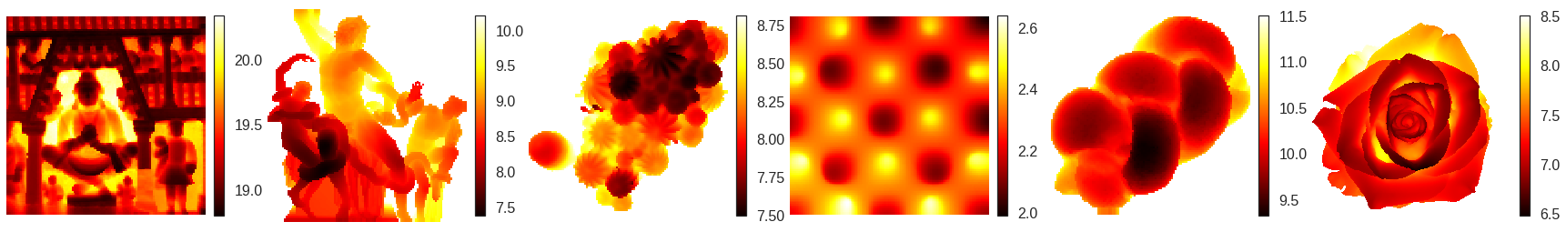
Santo et al.

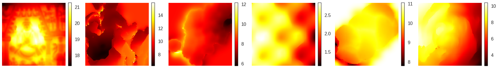
Peng et al.

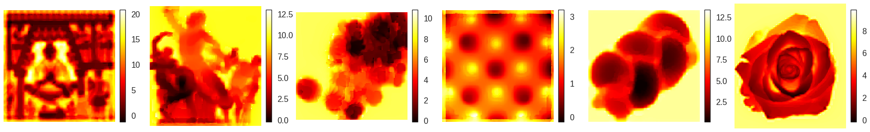
Ours

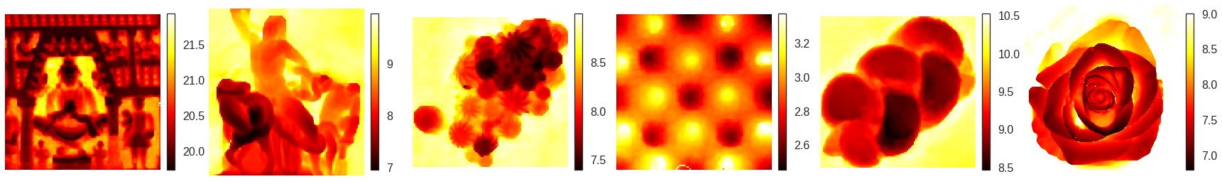
Figure 5: Comparison of depth maps. Each row refers to a specific method.

Relief Sculptures   Cactus Surface Bread Rose
Ground Truth
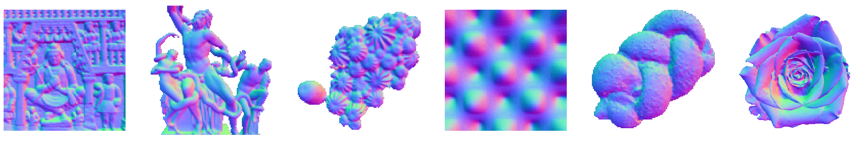
Santo et al.
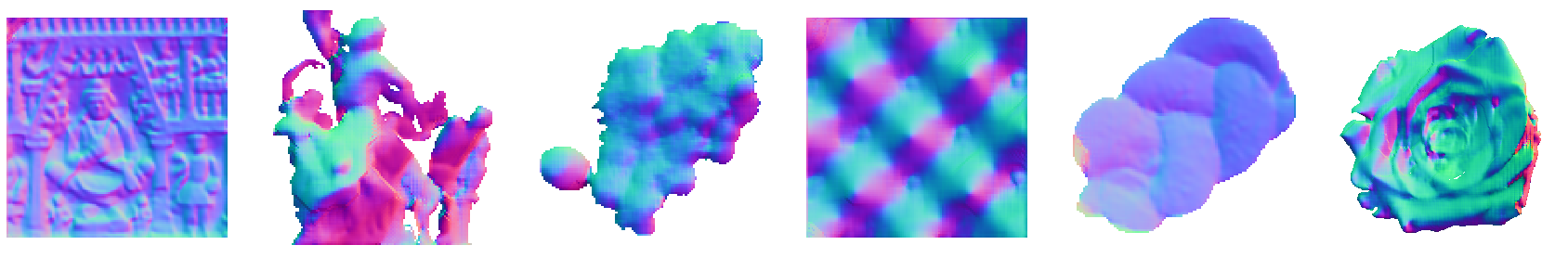
Chen et al.
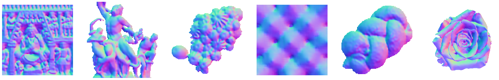
Ours

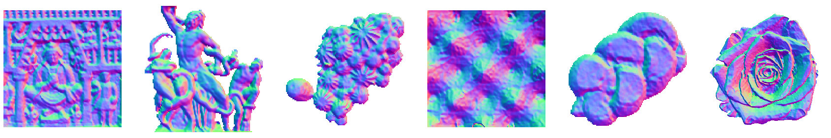
Figure 6: Comparison of surface normals estimated by each of the compared methods. Each row represents a different method.

4.3 Comparisons

We compare to the state-of-the-art methods of Chen et al. [5], Santo et al. [23], and Peng et al. [22], that use photometric stereo inputs, with the latter requiring a down-sampled depth map as an additional input. We compare both depth maps [22, 23] and normals [5, 23] (according to the generated outputs of each method).

Figure 5 shows a qualitative evaluation of depth map result quality. The method of Santo et al. produces a low frequency estimation of depth, but does not contain any high frequency details. The method of Peng et al. produces results which are closer to the ground truth, but still lacking in sharpness (e.g., in Relief and Cactus). Our method is overall closest to the ground truth depth. Quantitatively, we measure normalized mean depth error (nMZE) in Table 1. We achieve lower nMZE on 5 out of the 6 objects, with an overall average nMZE which is 1.7 times [22] and 4.9 times [23] lower than the alternative.

Figure 6 shows a qualitative evaluation of surface normal result quality. The method of Santo et al. produces overly smooth normals, with some examples relatively close to the ground truth (e.g., Relief) but others farther away (e.g., Rose). The method of Chen et al. is comparable to ours, with generally good results that resemble the ground truth normals, but lack sharp transitions. Quantitatively, we measure mean angle error (MAE in degrees) in Table 1. Our results are comparable to (albeit slightly better than) those of Chen et al., and 1.6 times better than those of Santo et al.

Table 1: Quantitative evaluation. The top three rows are depth map results, and the bottom rows are surface normal results. All methods but Peng et al. were given ground-truth light location, and Peng et al. was given a down-scaled depth map.

Method	Metric	Cactus	Rose	Bread	Sculptures	Surface	Relief	Avg
Santo et al. [23]	nMZE	0.96	1.16	0.77	0.81	0.75	0.75	0.87
Peng et al. [22]	nMZE	0.43	0.05	0.40	0.20	0.33	0.42	0.31
Chen et al. [5]	nMZE	N/A	N/A	N/A	N/A	N/A	N/A	N/A
Ours	nMZE	0.33	0.11	0.16	0.19	0.10	0.18	0.18
Santo et al. [23]	MAE	32.79	50.23	33.95	54.49	22.21	21.93	35.93
Peng et al. [22]	MAE	N/A	N/A	N/A	N/A	N/A	N/A	N/A
Chen et al. [5]	MAE	24.61	25.12	18.31	26.43	18.91	25.46	23.14
Ours	MAE	22.60	26.27	20.43	27.50	17.16	21.80	22.63

Table 2: Comparison of surface normal estimation on the dome dataset in [15] using calibrated methods (known light locations). Compared results were used from the original paper.

Method	Metric	Vase	Golf Ball	Face
Chen et al. [3]	MAE	27.11	15.99	16.17.81
Kaya et al. [15]	MAE	16.40	14.23	14.24
Ours	MAE	11.24	16.51	18.70

Table 3: Average shadow pixels in image analysis. We measure MAE of estimated surface normals for increasing amount of average shadows. These are calculated by taking the average amount of shadowed pixels in each rendered object.

Avg. Shadow	A(48%)	B(60%)	C(66%)	D(69%)	E(60%)*	Avg
Chen et al. [5]	18.63	18.71	20.43	21.44	22.99	20.44
Santo et al. [23]	16.18	17.25	17.19	18.25	42.70	22.31
Ours	20.43	18.53	17.95	17.53	18.68	18.62

Note that [15] refers to a rose object as an object with ‘complex geometry and high amount of surface discontinuity’, where their method fails due to their assumption of a continuous surface and due to a high amount of cast shadows. We render a similar object and show that our method does not require such assumptions. Visual results can be seen in Figure 1.

Besides our own generated dataset, we compare our results to three different shape-from-shading results reported in [15] which can be seen in Table 2. Since the vase object is concave, it has a strong cast shadow affect, which is a strong learning signal. We can also see that the shape-from-shading methods fail to deal with this. The golf and face objects have sparse cast shadows, which is likely the reason why our method does not perform well there.

4.4 Analysis & Ablation

Performance on various shadow amounts To further test our method, we generated the surface object using 16 lights placed at different incidence angles, thus creating inputs with increasing amount of shadows. We rendered this by placing the object at a constant location, and increasing the distance of the lights from the object at each different scene. We observe in Table 3 that DeepShadow’s accuracy improves as the amount of shadow present in the image increases, as opposed to the other tested methods, in which the accuracy degrades as the amount of shadowed pixels increases. Note that objects A–D were rendered with lights at a constant distance, and object E was rendered with lights at varying distances. We observe that [23] does not handle this scenario well.

Cactus Surface Bread
Depth map error
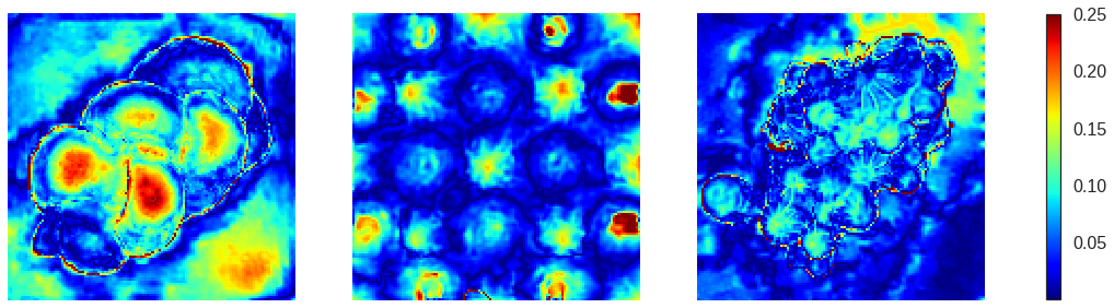
Sum of shadowed pixels

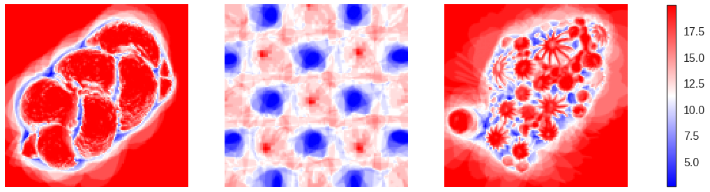
Figure 7: Comparison of Depth Estimation Error (top) vs. Number of Shadowed Pixels (bottom). In the bottom row, we can observe pixels that are mostly shadowed (blue) or mostly illuminated (red) in all renderings. These pixels have higher depth estimation errors (top row). Pixels that are balanced, i.e., shadowed and illuminated in roughly equal proportions (white, bottom row) have a smaller depth estimation error.

Shadowed and illuminated pixels. We analyze the effects of the number of shadowed and illuminated pixels on the final depth estimation. In Figure 7 we compare the error map (top) to the number of illuminated pixels across all lighting conditions (bottom). Our method works best if this sum is balanced, i.e., if pixels are illuminated in some samples and shadowed in other samples. If pixels are always shadowed or always illuminated, reconstruction is ill-posed and our method does not perform well.

4.5 Failure Cases

Our algorithm is based on the line of sight algorithm, thus it relies on shadow gradients to reconstruct the underlying depth map. In objects such as the face in Table 2, the algorithm fails in flat areas, e.g., as the forehead, since the latter is relatively smooth and convex - and thus has no shadow from which to learn from. This is also true for the bread object in Table 1, which has large areas that are flat, as can be seen in Figure 7. In contrast, the vase in Table 2 is relatively smooth yet also concave, and has many cast shadows, which enables our method to succeed.

5 Conclusions

In this work we proposed DeepShadow, a deep-learning based method for recovering shape from shadows. We show that in various scenarios, the shadow maps serve as good learning signals that enable the underlying depth and surface normals to be recovered. Experiments have shown that this method achieves results equal to or better than those generated by the various shape-from-shading algorithms, for severely shadowed objects, while using fewer or no data — since we are not using any training data besides the shadow maps. An additional benefit of our method is that we do not require knowing the light intensity, since the shadow maps are of binary values. Even though previous works have shown this can be estimated, the estimation may be erroneous, which affects the final result.

Our method fails on convex objects or objects with sparse shadows. In future work, this method should be combined with shape-from-shading methods in order for both methods to benefit from each other. Another possible research direction is producing super-resolution depth maps using the shadow clues, which would combine our work and [22]. Since we are using implicit representations, this may work well.

5.0.1 Acknowledgements

This work was supported by the Israeli Ministry of Science and Technology under The National Foundation for Applied Science (MIA), and by the Israel Science Foundation (grant No. 1574/21).

Appendix 0.A Shadow and light extraction network

Since shadow maps are not always available, we train a network to estimate them from input photometric stereo images. This network runs as a pre-processing step on the photometric stereo data, to produce shadow maps that DeepShadow can use as inputs. Our model also estimates the light direction, since this is also not always available. We use both a publicly available photometric stereo dataset, as well as our own renders — which are needed since there is no public dataset that has photometric stereo shadow ground-truth.

Please note that our goal is estimating depth from shadow maps. As we have shown, in certain cases DeepShadow with shadow maps as inputs may result in better shape estimation than shape-from-shading techniques. We trained the shadow and light extraction model solely to be able to use our method on datasets which do not have ground-truth shadow maps or light directions, so that we are able to test our method on more types of objects and scenes. Using the light extraction model, we estimate the direction of lights (located at infinity), and then convert these to point-lights by projecting onto the unit sphere and multiplying by a constant, empirically set to twice the distance between camera and object.

0.A.1 Network Architecture

The shadow estimation model is illustrated in Figure A1. It is used for estimating light directions and shadow maps given photometric stereo image inputs. Although the model also outputs normal maps, these are only used during the training and are discarded during the inference. The input images have dimensions of $S\times C\times W\times H$, $S$ being the number of input images (sequence dimension), $C$ is the image color channel, and $H\times W$ is the spatial image size.

The complete model is composed of four hybrid Transformer-Convolution layers (ConvTransformers): the first block is a ConvTransformer for extracting features from the input images, and the second and third blocks are two ConvTransformers for estimating shadows and for estimating light directions. The last custom block is used for estimating the normals from the features (not illustrated in Figure A1).

The feature-extraction ConvTransformer splits each input image into an 8x8 patch, as applied in Vision Transformer (ViT) [11]. In contrast to the regular ViT, we group all patches along the sequence dimension, since the main target of the model is predicting per-pixel output for each patch. Since predicting shadows from photometric stereo images is essentially a threshold-based problem, we choose to use an attention-based model and compare all spatially co-located patches, instead of comparing all patches in a single image. These patches are then used as a sequence of inputs to the transformer. Each sequence is passed separately through a ConvTransformer (sequences can be batched together) to produce a sequence of intermediate features extracted from the relevant patches. Once all the patches have passed through the transformer, they are reshaped back to the original image dimensions, and then passed through a convolution layer to output the features. The feature-extraction ConvTransformer is composed of 4 Transformer-Convolution pairs, with 16 attention heads and latent MLP dimension of 1024.

The light direction block uses 2 ConvTransformer blocks, with a 128 dim MLP and 4 attention heads. The shadow estimation block uses 3 ConvTransformer blocks with 6 attention heads and an MLP dimension of 128. It utilizes a Sigmoid function for outputting values between 0 and 1. We also estimate the surface normals from the features, using a linear projection layer and two convolution layers. This is done in order to be able to learn from datasets which have photometric stereo data and ground-truth normals.

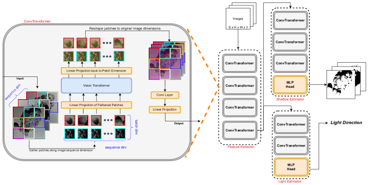
Figure A1: Shadow Estimation Model. The model receives as inputs a sequence of photometric stereo images and outputs the estimated light directions and shadow maps. Each image is split to patches, and patches are gathered by the sequence index. Each such sequence is fed separately to the ConvTransformer. The model is composed of a four layer ConvTransformer which outputs intermediate features. These features are used to generate the final outputs, using 2 smaller ConvTransformers. The ConvTransformer can be viewed in detail in the bottom of the figure.

0.A.2 Training Details

We use the Blobby and Sculptures datasets [3], which contain photometric stereo images, light directions and surface normals. We also render a shadow dataset composed of 10 objects downloaded from Sketchfab. Each object was rendered in 32 different view angles and with 32 light angles for each view. We use Blender [8] to render our datasets. We use all three datasets during training in a ratio of 1:1:10, i.e., for every 10 iterations over the shadow dataset, we iterate once over the Blobby and Sculptures datasets.

During training, we randomly crop each input images to $64\times 64$. We use random noise and color jitter augmentations, as well as randomize the sequence length between 16 and 32 inputs, in order to make the transformer agnostic to the number of input images.

We use the following loss function:

$$\mathcal{L}=\frac{1}{M}\sum_{m}\left(\mathcal{L}_{N}^{m}+\mathcal{L}_{S}^{m}+\mathcal{L}_{L}^{m}\right)$$ (A1)

where $\mathcal{L}_{N}^{m}$ is the normal loss, $\mathcal{L}_{S}^{m}$ is the shadow reconstruction loss and $\mathcal{L}_{L}^{m}$ is the light direction loss. The sum is performed over all $m\in[0,M]$ sets of photometric images in the dataset. Each such set has $k\in[0,K]$ images of size $H\times W$ along with the associated light directions $\ell_{k}$ and a ground-truth normal map $N$. Our rendered dataset also has ground-truth shadow maps $S_{k}$. The complete loss combines between the loss of the ground-truth normals $N$ and the predicted normals $\hat{N}$,

$$\mathcal{L}_{N}^{m}=\frac{1}{HW}(1-N^{m}\cdot\hat{N}^{m}),$$ (A2)

the L1 loss of the ground-truth and predicted shadow maps

$$\mathcal{L}_{S}^{m}=\frac{1}{KHW}\sum_{k}|S^{m}_{k}-\hat{S}^{m}_{k}|,$$ (A3)

and the cosine embedding loss between the ground-truth light direction $\ell^{m}_{k}$ and the estimated direction $\hat{\ell}^{m}_{k}$

$$\mathcal{L}_{L}^{m}=\frac{1}{K}\sum_{k}(1-cos(\ell^{m}_{k},\hat{\ell}^{m}_{k})).$$ (A4)

We omit the supervision on the lights when using our dataset, and omit the shadow supervision when using Blobby and Scupltures datasets. We train using the Adam optimizer [16] for 1000 epochs with an initial learning rate of $1\times 10^{-4}$ which is decreased by a factor of 0.8 every 15 epochs.

The results of the shadow estimation can be seen in Figure A2.

Input Images

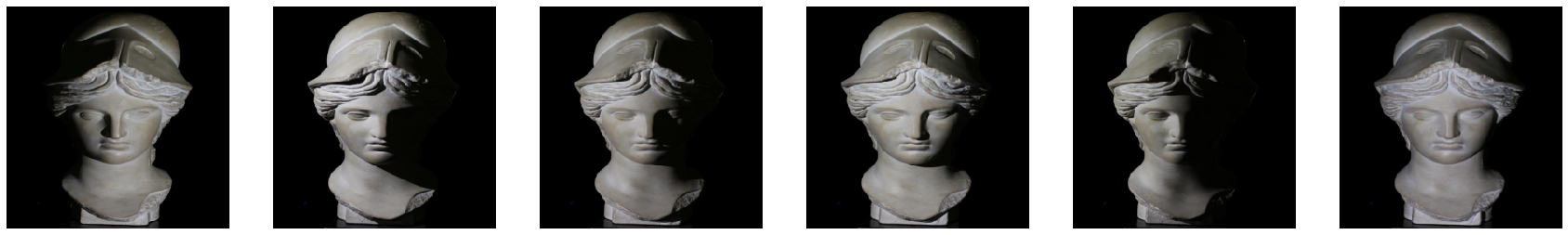
Est. Shadows

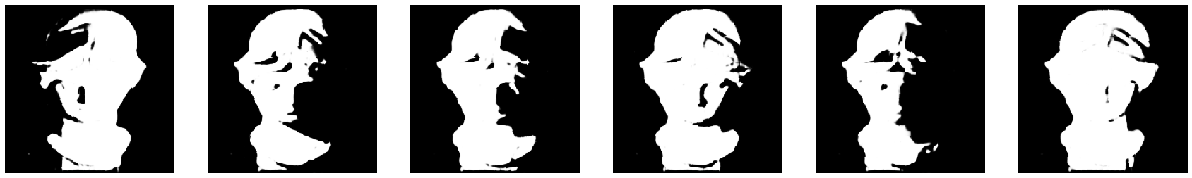
Figure A2: Sculpture head object shadow estimation results.

Appendix 0.B Additional Results

In this section, we present more results of the DeepShadow method. We also examine the performance of the shadow estimation network on data which lacks ground-truth shadows.

0.B.1 Normal map errors

Figure A3 shows the previously shown objects’ normal map errors. Our method produces less normal errors on the Relief, Cactus, Surface and Rose objects compared to other methods.

	Relief	Sculptures	Cactus	Surface	Bread	Rose
Santo et al.
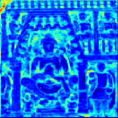
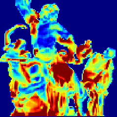
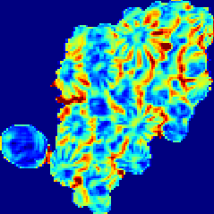
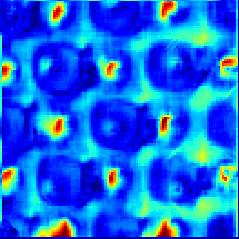
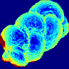
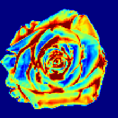
Chen et al.
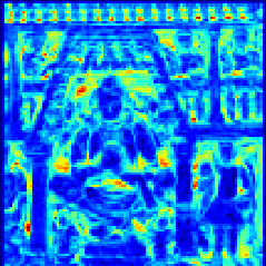
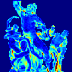
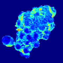
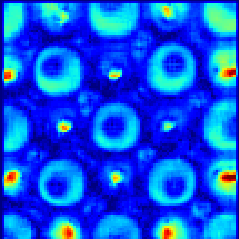
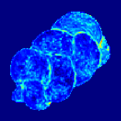
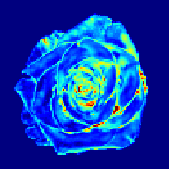
A.Ours

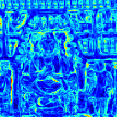
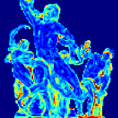
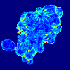
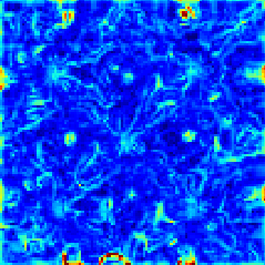
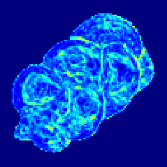
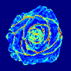
Figure A3: Normal error maps comparing our method to [5] and [23].

0.B.2 Specular and diffuse objects

We test our method’s resiliency to specular inputs and compare to that of a shape-from-shading method. We rendered a modified version of our rose object, with two different materials; highly specular and diffuse (Figure A4).

Diffuse Obj.	Specular Obj.	SDPS Diff.	SDPS Spec.	Ours Diff.	Our Spec.

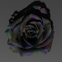
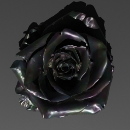
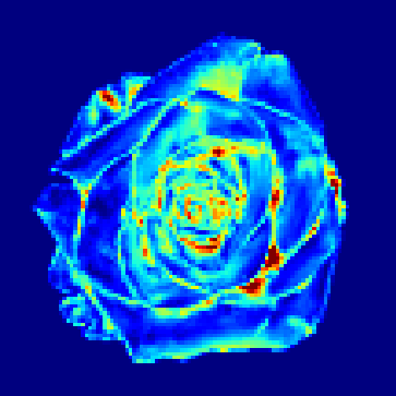
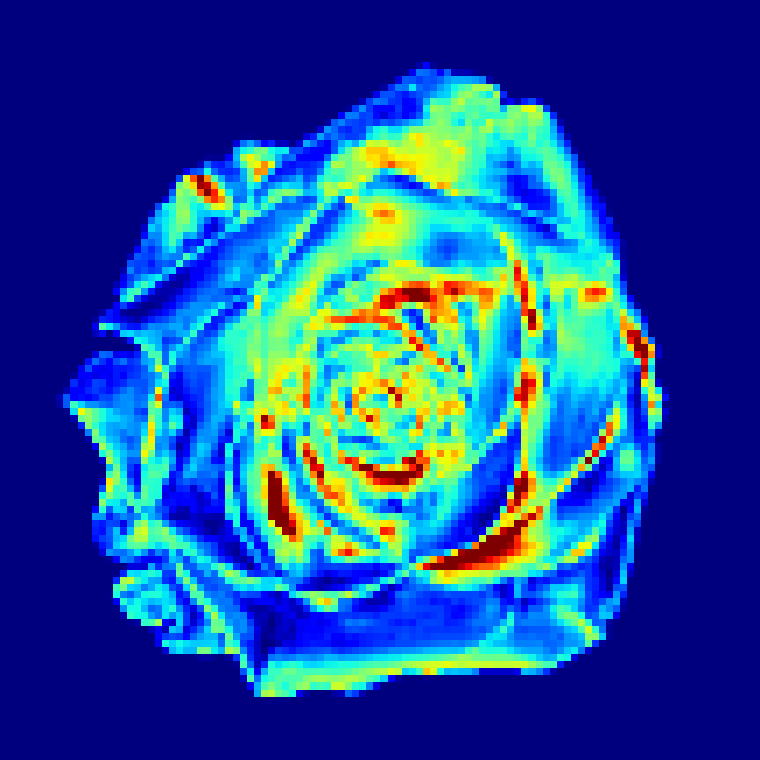
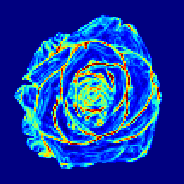
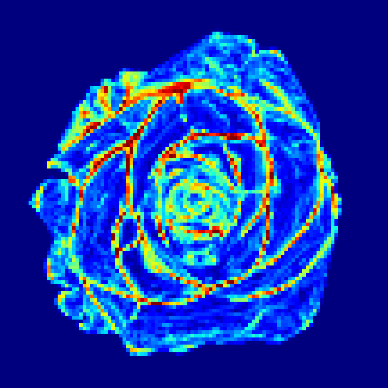
Figure A4: Effect of specularities on angle error of output normals.

We evaluated our algorithm (including the shadow extraction model) on these objects, and compared the surface normal results to SDPS [5]. The diffuse object produces 25.02 MAE and the metallic object produces 34.35 MAE using SDPS, while our method achieves 26.50 MAE and 27.76 MAE, respectively. With specularity added, we can see a big drop in accuracy using SDPS, while our method achieves a smaller drop.

0.B.3 Shadow maps reconstruction error

We present the shadow reconstruction error on two objects from our rendered dataset. The reconstruction has two types of errors. The first is due to the nearest neighbor rounding used for the boundary sampling in the R2 method, and can be seen clearly in the third row cactus’ shadow error, in the upper area, and in the surface’s second, third and sixth rows. The second error can mostly be seen in the edges of the objects (e.g., last row in Figure A5). The source of the error are edges in the depth map. Recall we generate a shadow line scan from the light source to each boundary pixel, and estimate the depth map value for every pixel in the image. The error can be minimized by sampling each line in a denser fashion rather than sampling a coordinate for every pixel, although it would come at a cost of computational cost.

GT Shadows

Est. Shadows

Shadow Error

GT Shadows

Est. Shadows

Shadow Error

Figure A5: Shadow reconstruction error. The top 3 rows are from the cactus object and the bottom 3 rows are from the surface object. Ground-truth and estimated shadows are shown, along with the L1 error between them. Each column represents a different illumination direction.

0.B.4 Results on objects from Dome dataset

We present our results on vase, face and golf ball objects from the Dome dataset [15]. The vase results can be seen in Figure A6. Previous shape-from-shadow methods [10, 24, 32] have used a threshold on gray-scale images to estimate shadows from images. As can be seen in Figure A6, simple thresholds fail on an object such as the vase, which has specular highlights. We show the results for 3 different thresholds by taking values of 0.4, 0.5 and 0.6. Each threshold fails to produce accurate shadow maps in specific areas.

We also show our depth and normal estimation results in Figure A7, which have been discussed in the main paper.

Light 1 Light 2 Light 3 Light 4 Light 5 Light 6
Input Images

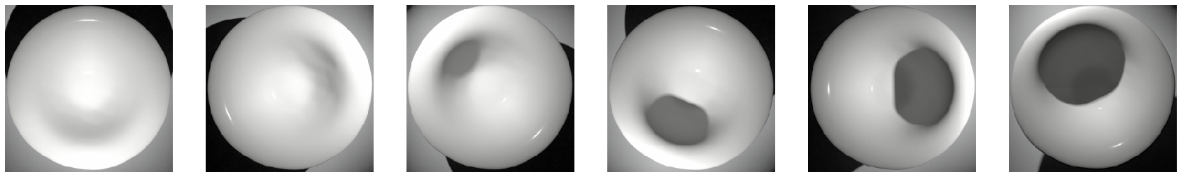
Est. Shadows

Threshold=0.4

Threshold=0.5

Threshold=0.6

Figure A6: Vase object shadow estimations. The top row contains the input images, the second row is our estimated shadow results using the model described in Appendix 0.A. The three bottom rows are a baseline result by taking thresholds of 0.4, 0.5 and 0.6 over the grayscale levels. Each column is a different light direction. A threshold of 0.4 fails on light directions 2, 3, and 4; a threshold of 0.5 fails on light directions 2 and 6 (external region); a threshold of 0.6 fails on light directions 4, 5, and 6.

GT normals      Estimated normals     Normal error map     Estimated Depth
Vase

Golf ball

Face

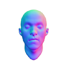
Figure A7: Results on objects from [15]. Each row (from left to right) consists of ground-truth normals, estimated normals, normal error map and estimated depth. As described in the paper, the results of DeepShadow on the vase object outperform other attempted methods. The normal map produced from the golf ball has errors around the edges. The face’s estimated normal map has errors mostly around the forehead area, since that area is smooth and sparse in shadows.

0.B.5 Results on real object

We present qualitative results on the hand and statue in Figure A8. The objects were acquired in a half-dome setting with 34 different illuminations. Ground truth normals and depth are not available on this dataset, as well as light directions, which were estimated using the model described in Appendix 0.A. Our method requires the intrinsic camera parameters which were not known, thus had to be roughly estimated by guessing the object’s size, and assuming a typical 50mm focal length.

Hand Images

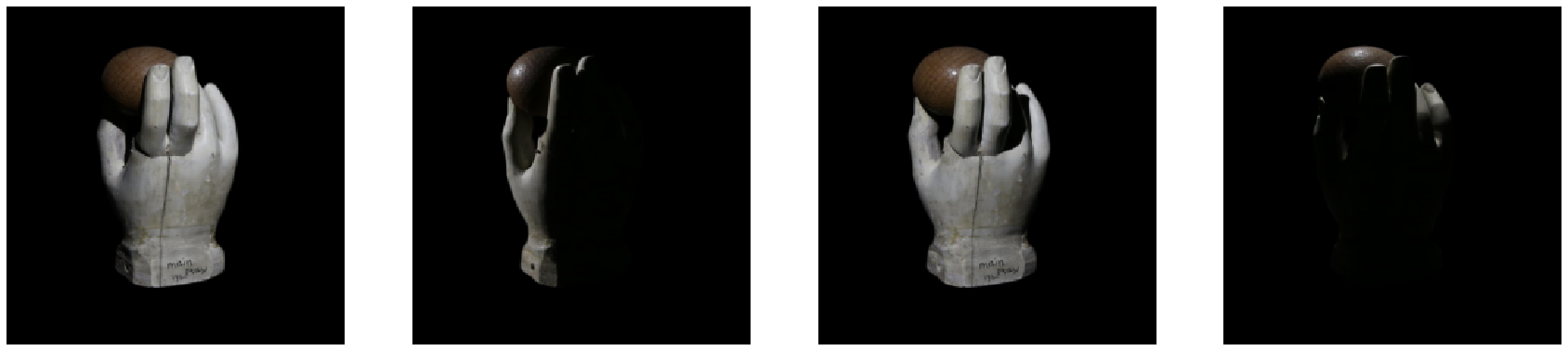
Hand Shadows

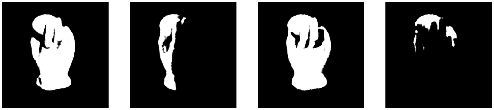
Estimated Results

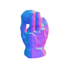
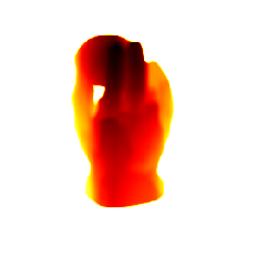
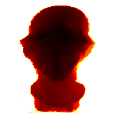
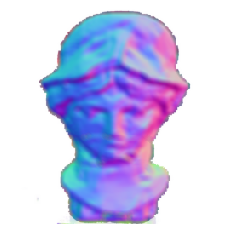
Statue Shadows

Statue Images

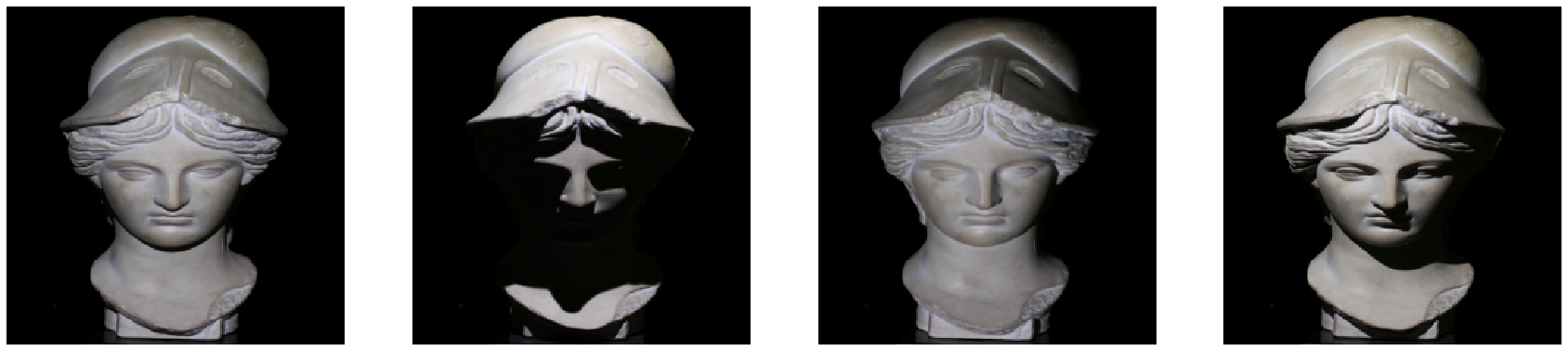
Figure A8: Input images, shadows, estimated depth and normals. The upper row includes the hand object images, and the second row their estimated shadows. The third row contains the estimated depth and surface normals of both objects. The fifth row includes the statue image inputs and the forth row their estimated shadow maps. We can observe DeepShadow is able to extract fine detail in areas such as the helmet and hair of the statue, and fails in smooth areas such as its neck.

References

- [1] Mark Boss et al. “NeRD: Neural Reflectance Decomposition from Image Collections” In IEEE International Conference on Computer Vision (ICCV), 2021
- [2] Manmohan Chandraker, Sameer Agarwal and David Kriegman “ShadowCuts: Photometric Stereo with Shadows” In 2007 IEEE Conference on Computer Vision and Pattern Recognition, 2007, pp. 1–8 DOI: 10.1109/CVPR.2007.383288
- [3] Guanying Chen, Kai Han and Kwan-Yee K. Wong “PS-FCN: A Flexible Learning Framework for Photometric Stereo” In ECCV, 2018
- [4] Guanying Chen et al. “Deep Photometric Stereo for Non-Lambertian Surfaces”, 2020 arXiv:2007.13145 [cs.CV]
- [5] Guanying Chen et al. “Self-calibrating Deep Photometric Stereo Networks”, 2019 arXiv:1903.07366 [cs.CV]
- [6] Guanying Chen et al. “What Is Learned in Deep Uncalibrated Photometric Stereo?” In Computer Vision – ECCV 2020 Cham: Springer International Publishing, 2020, pp. 745–762
- [7] Richard Cole and Micha Sharir “Visibility problems for polyhedral terrains” In Journal of symbolic Computation 7.1 Elsevier, 1989, pp. 11–30
- [8] Blender Online Community “Blender - a 3D modelling and rendering package”, 2018 Blender Foundation URL: http://www.blender.org
- [9] M. Daum and G. Dudek “On 3-D surface reconstruction using shape from shadows” In Proceedings. 1998 IEEE Computer Society Conference on Computer Vision and Pattern Recognition (Cat. No.98CB36231), 1998, pp. 461–468 DOI: 10.1109/CVPR.1998.698646
- [10] M. Daum and G. Dudek “On 3-D surface reconstruction using shape from shadows” In Proceedings. 1998 IEEE Computer Society Conference on Computer Vision and Pattern Recognition (Cat. No.98CB36231), 1998, pp. 461–468 DOI: 10.1109/CVPR.1998.698646
- [11] Alexey Dosovitskiy et al. “An Image is Worth 16x16 Words: Transformers for Image Recognition at Scale” In CoRR abs/2010.11929, 2020 arXiv: https://arxiv.org/abs/2010.11929
- [12] Wm Randolph Franklin and Clark Ray “Higher isn’t necessarily better: Visibility algorithms and experiments” In Advances in GIS research: sixth international symposium on spatial data handling 2, 1994, pp. 751–770 Taylor & Francis Edinburgh
- [13] Michael F Goodchild and Jay Lee “Coverage problems and visibility regions on topographic surfaces” In Annals of Operations Research 18.1 Springer, 1989, pp. 175–186
- [14] Bjoern Haefner et al. “Photometic Depth Super-Resolution” In IEEE Transactions on Pattern Analysis and Machine Intelligence, 2019
- [15] Berk Kaya et al. “Uncalibrated Neural Inverse Rendering for Photometric Stereo of General Surfaces”, 2021 arXiv:2012.06777 [cs.CV]
- [16] Diederik P. Kingma and Jimmy Ba “Adam: A Method for Stochastic Optimization”, 2017 arXiv:1412.6980 [cs.LG]
- [17] Fotios Logothetis, Ignas Budvytis, Roberto Mecca and Roberto Cipolla “A CNN Based Approach for the Near-Field Photometric Stereo Problem”, 2020 arXiv:2009.05792 [cs.CV]
- [18] Fotios Logothetis, Ignas Budvytis, Roberto Mecca and Roberto Cipolla “PX-NET: Simple and Efficient Pixel-Wise Training of Photometric Stereo Networks”, 2021 arXiv:2008.04933 [cs.CV]
- [19] Linjie Lyu et al. “Efficient and Differentiable Shadow Computation for Inverse Problems” In Proceedings of the IEEE/CVF International Conference on Computer Vision (ICCV), 2021, pp. 13107–13116
- [20] Ben Mildenhall et al. “NeRF: Representing Scenes as Neural Radiance Fields for View Synthesis” In ECCV, 2020
- [21] Adam Paszke et al. “PyTorch: An Imperative Style, High-Performance Deep Learning Library” In Advances in Neural Information Processing Systems 32 Curran Associates, Inc., 2019, pp. 8024–8035 URL: http://papers.neurips.cc/paper/9015-pytorch-an-imperative-style-high-performance-deep-learning-library.pdf
- [22] Songyou Peng, Bjoern Haefner, Yvain Quéau and Daniel Cremers “Depth Super-Resolution Meets Uncalibrated Photometric Stereo” In IEEE International Conference on Computer Vision (ICCV) Workshop, 2017
- [23] Hiroaki Santo, Michael Waechter and Yasuyuki Matsushita “Deep Near-Light Photometric Stereo for Spatially Varying Reflectances” In Computer Vision – ECCV 2020 Cham: Springer International Publishing, 2020, pp. 137–152
- [24] Silvio Savarese et al. “3D Reconstruction by Shadow Carving: Theory and Practical Evaluation” In International Journal of Computer Vision 71, 2007, pp. 305–336 DOI: 10.1007/s11263-006-8323-9
- [25] Andrew Shapira “Visibility and terrain labeling”, 1990
- [26] Vincent Sitzmann et al. “Implicit Neural Representations with Periodic Activation Functions” In Proc. NeurIPS, 2020
- [27] Pratul P. Srinivasan et al. “NeRV: Neural Reflectance and Visibility Fields for Relighting and View Synthesis”, 2020 arXiv:2012.03927 [cs.CV]
- [28] Tatsunori Taniai and Takanori Maehara “Neural Inverse Rendering for General Reflectance Photometric Stereo”, 2018 arXiv:1802.10328 [cs.CV]
- [29] Robert J. Woodham “Photometric Method For Determining Surface Orientation From Multiple Images” In Optical Engineering 19.1 SPIE, 1980, pp. 139–144 DOI: 10.1117/12.7972479
- [30] Yukihiro Yamashita, Fumihiko Sakaue and Jun Sato “Recovering 3D Shape and Light Source Positions from Non-planar Shadows” In 2010 20th International Conference on Pattern Recognition, 2010, pp. 1775–1778 DOI: 10.1109/ICPR.2010.1153
- [31] Zhuokun Yao et al. “Gps-net: Graph-based photometric stereo network” In Advances in Neural Information Processing Systems 33, 2020
- [32] Yizhou Yu and Johnny Chang “Shadow Graphs and 3D Texture Reconstruction” In International Journal of Computer Vision 62, 2005, pp. 35–60 DOI: 10.1023/B:VISI.0000046588.02227.3b
- [33] Huangying Zhan, Chamara Saroj Weerasekera, Ravi Garg and Ian D. Reid “Self-supervised Learning for Single View Depth and Surface Normal Estimation” In CoRR abs/1903.00112, 2019 arXiv: http://arxiv.org/abs/1903.00112
- [34] Xiuming Zhang et al. “NeRFactor” In ACM Transactions on Graphics 40.6 Association for Computing Machinery (ACM), 2021, pp. 1–18 DOI: 10.1145/3478513.3480496