are or etc Online Algorithms for Matching Platforms with Multi-Channel Traffic MS-RMA-22-00910.R1

Manshadi et al.

Algorithms for Multi-Channel Traffic

Vahideh Manshadi Yale School of Management, New Haven, CT, vahideh.manshadi@yale.edu Scott Rodilitz University of California - Los Angeles, Los Angeles, CA, scott.rodilitz@anderson.ucla.edu Daniela Saban Stanford Graduate School of Business, Stanford, CA, dsaban@stanford.edu Akshaya Suresh Yale School of Management, New Haven, CT, akshaya.suresh@yale.edu

Two-sided platforms rely on their recommendation algorithms to help visitors successfully find a match. However, on platforms such as VolunteerMatch – which has facilitated millions of connections between volunteers and nonprofits – a sizable fraction of website traffic arrives directly to a nonprofit’s volunteering page via an external link, thus bypassing the platform’s recommendation algorithm. We study how such platforms should account for this external traffic in the design of their recommendation algorithms, given the goal of maximizing successful matches. We model the platform’s problem as a special case of online matching, where (using VolunteerMatch terminology) volunteers arrive sequentially and probabilistically match with one opportunity, each of which has finite need for volunteers. In our framework, external traffic is interested only in their targeted opportunity; by contrast, internal traffic may be interested in many opportunities, and the platform’s online algorithm selects which opportunity to recommend. In evaluating the performance of different algorithms, we refine the notion of competitive ratio by parameterizing it based on the amount of external traffic. After demonstrating the shortcomings of a commonly-used algorithm that is optimal in the absence of external traffic, we propose a new algorithm – Adaptive Capacity (AC) – which accounts for matches differently based on whether they originate from internal or external traffic. We provide a lower bound on AC’s competitive ratio that is increasing in the amount of external traffic and that is close to (and, in some regimes, exactly matches) the parameterized upper bound we establish on the competitive ratio of any online algorithm. We complement our theoretical results with a numerical study motivated by VolunteerMatch data where we demonstrate the strong performance of AC relative to current practice and further our understanding of the difference between AC and other commonly-used algorithms.

matching platforms, online algorithms, competitive analysis, multi-channel traffic

1 Introduction

Online platforms have become increasingly prominent in facilitating social and economic connections in both the private and nonprofit sectors. In the private sector, the e-commerce platform Etsy has empowered over 2 million small-scale sellers to showcase their products to over 40 million buyers and has facilitated transactions on the scale of $4 billion. In the nonprofit sector, the crowdfunding platform DonorsChoose has helped public school teachers to successfully solicit $314 million in donations for 1.7 million classroom projects. Similarly, VolunteerMatch has enabled over 18 million connections between organizations and individuals looking for volunteering opportunities.

These platforms attract traffic through multiple channels. Some users organically visit the platform and rely on its recommendation algorithm to find a desired product or volunteering opportunity—we refer to these users as internal traffic. Other users, which we refer to as external traffic, follow an external direct link to a particular page. This external traffic is generated through a variety of off-platform outreach mechanisms, such as posting on social media or sending customized notifications. For example, an artist who sells their handmade products on Etsy may tweet about them, or an NGO may publicize their volunteering/donation opportunities on their Facebook page. In this paper, we aim to understand how these matching platforms can efficiently leverage traffic from all sources in order to maximize the number of successful transactions/connections.

This work is partly motivated by our collaboration with VolunteerMatch (VM), the largest nationwide platform that connects nonprofits with volunteers. More than 130,000 organizations—supporting a variety of social causes, ranging from human rights and literacy to helping seniors—have posted their volunteering opportunities on the VM website. Most of these organizations rely on volunteers who sign-up after browsing the VM website. Some of these organizations also generate sign-ups by publicizing their opportunities on other websites, such as LinkedIn or Facebook. Our analysis of VM data reveals two key facts. First, a significant portion of volunteer sign-ups come from external traffic: for example, 30% of all sign-ups made by NYC-based volunteers between August 1, 2020 and March 1, 2021 came from external traffic. Second, there is a significant disparity across opportunities in terms of both the total number of sign-ups and the source of those sign-ups.

Figure 1: Distribution of sign-ups on VM across a subset of opportunities requesting 5 volunteer sign-ups.

To illustrate these two facts, in Figure 1 we plot the distribution of the number of sign-ups for a subset of opportunities that all requested 5 volunteer sign-ups. Partitioning the sign-ups into two groups based on their source, we observe that the volume of sign-ups from external traffic (in purple) and from internal traffic (in green) varies substantially across opportunities. From the platform’s perspective, a key difference between external and internal traffic comes from whether or not the user’s choice can be influenced: the platform cannot control the “landing page” for external traffic, but it can impact what internal traffic views (and thus the decisions made) via its recommendation algorithm. Through its search design, the platform can (potentially) re-distribute “excessive” sign-ups from internal traffic (i.e., sign-ups that exceed an opportunity’s need) to opportunities with insufficient sign-ups, thereby helping VM achieve its strategic goal of maximizing the total number of “useful” sign-ups across opportunities. For instance, for the subset of opportunities presented in Figure 1, in hindsight, $49\%$ of sign-ups from internal traffic (the dashed green portions of the bars) could potentially have been re-directed to opportunities with insufficient sign-ups.

The above observations motivate our main research question: how can matching platforms, such as VM, integrate external and internal traffic to maximize the number of useful sign-ups? As the traffic pattern is generally unknown a priori and there is heterogeneity in the level of external traffic, making better real-time recommendations to internal traffic may be challenging.

1.1 Our Contributions

To study the above question, we introduce a framework for online matching with multi-channel traffic. Taking a competitive analysis approach, we show that existing algorithms—that are optimal in the absence of external traffic—fail to integrate such traffic efficiently; thus, we develop a new algorithm that effectively incorporates external traffic, resulting in near-optimal guarantees in certain regimes. Beyond worst-case guarantees, we illustrate the effectiveness of our algorithm in a simulation study calibrated on VM data. We describe each contribution in more detail next.

A model for online matching with multi-channel traffic: For concreteness, we utilize terminology from the context of VM and refer to the two sides of the matching platform as “opportunities” and “volunteers.” In our setting, a fixed set of opportunities are posted on the platform, each requiring a certain number of volunteers which we refer to as its “capacity.” Volunteers arrive sequentially (in an arbitrary order) and are either external or internal traffic. External traffic directly views a specific opportunity’s page and signs up for it. By contrast, internal traffic can be influenced by the platform’s recommendation algorithm as follows. When an internal traffic volunteer arrives, the platform observes their conversion probability for each opportunity (i.e., the probability that the volunteer signs up for that opportunity conditional on viewing it), and then must immediately and irrevocably recommend one such opportunity. The goal of the platform is to maximize the total number of “useful” sign-ups, i.e., the total number of sign-ups that don’t exceed an opportunity’s capacity.

In the absence of external traffic, the above problem can be viewed as an instance of the online bipartite B-matching problem with stochastic rewards and an adversarial arrival sequence. In this general framework, it has been shown that a simple myopic algorithm commonly-referred to as MSVV achieves the best-possible competitive ratio of $1-1/e$ (Mehta et al. 2007). We augment this framework by modeling external traffic as arrivals with only one possible edge (e.g., volunteers that only consider one opportunity). The presence of external traffic reduces the complexity of making real-time decisions: the platform cannot change what external traffic volunteers will view, as they are only interested in one opportunity. Thus, in the extreme case where all capacity can be filled by external traffic, the platform trivially maximizes the number of useful sign-ups.

In light of the above observation, we parameterize problem instances based on the fraction of total capacity that can be filled by external traffic, which we call the effective fraction of external traffic (EFET), as formalized in Definition 2. For a given EFET, we define the competitive ratio of an algorithm to be the worst-case ratio between its outcome and that of a benchmark, among all instances with that EFET (see Definition 3). Our benchmark (denoted OPT) is a clairvoyant solution that a priori knows the sequence of arrivals, but only observes the sign-up realizations of internal traffic after recommending an opportunity (see Definition 1). We study how the addition of external traffic improves the achievable competitive ratio.

Failure of channel-agnostic algorithms: To gain intuition, we first focus on a thought experiment where all of the external traffic arrives before any of the internal traffic. In such a setting, after the sign-ups from external traffic realize, the platform is faced with a standard instance of the online matching problem. Thus, by making recommendations in the remaining problem according to an optimal algorithm like MSVV, we would hope to achieve a competitive ratio that is a convex combination of $1$ and $1-1/e$. Indeed, in Proposition 1, we prove that this convex combination is an upper bound on any online algorithm. However, somewhat surprisingly, applying MSVV to the entire problem instance does not achieve this intuitive bound (Proposition 2). The suboptimality of this algorithm stems precisely from a lack of differentiation between external and internal traffic.

Adaptive Capacity (AC) algorithm: Building on the intuition developed in the thought experiment above, we introduce a new algorithm called Adaptive Capacity (AC) which reduces an opportunity’s capacity by one whenever that opportunity receives a sign-up from external traffic. If all external traffic arrives before any internal traffic, AC achieves the upper bound in Proposition 2. However, in a general setting where external traffic can arrive at arbitrary times, AC does not have the information needed to reduce capacities up-front; instead, it adaptively reduces capacity after each sign-up from external traffic (see Algorithm 2).

To shed light on the inherent difficulty of making real-time decisions under arbitrary arrival sequences, we first establish an upper-bound (as a function of the EFET) on the competitive ratio of any online algorithm (Theorem 1). Our main theoretical results establish performance guarantees (also as a function of the EFET) on the competitive ratio of AC that depend on the conversion probabilities (see Figures 2(b) and 2(c) for an illustration). In the special case with deterministic conversion, i.e., where conversion probabilities are either $0$ or $1$, we use combinatorial arguments inspired by the ideas of Mehta et al. (2007) to establish a lower bound on the performance of AC that converges to our upper bound as capacities increase (Theorem 2).

For more general settings, Theorem 3 parameterizes AC’s achievable competitive ratios by the maximum conversion probability ratio (MCPR), which we formally introduce in Definition 4. Fixing any MCPR and focusing on the large-capacity regime, our lower bound curve starts at $1-1/e$ (when there is no external traffic) but weakly increases with the EFET and eventually breaks the barrier of $1-1/e$. As the MCPR approaches $1$, our lower bound nearly matches our upper bound on AC for any EFET. The lower bounds that we establish on the competitive ratio of AC compare favorably to the competitive ratio of MSVV, which we show is strictly worse in some regimes. Beyond worst-case guarantees, in Section 4.3 we provide insight into instance characteristics that favor one algorithm over the other.

Our theoretical results are particularly intriguing because our algorithm does not require a priori knowledge of the volume of external traffic; yet by adaptively reducing capacities, AC achieves a near-optimal (and in some settings, exactly optimal) competitive ratio. This is an appealing quality for practitioners, as it is often infeasible to know the volume of external traffic in advance. Moreover, for high-information settings where practitioners have advance knowledge about the volume of external traffic per opportunity, we describe how a variant of AC can attain stronger performance guarantees (see Remark 1).

To analyze the competitive ratio of AC in the general case, we build on the LP-free approach in Goyal et al. (2020), which establishes a system of inequalities involving path-based “pseudo-rewards.” To break the barrier of $1-1/e$ we leverage the observation that an algorithm cannot make a bad decision for external traffic, and thus we define pseudo-rewards based on the source of the traffic. Moreover, as the volume of external traffic varies across opportunities, we move beyond an opportunity-level analysis, and instead bound the “global” value of AC relative to OPT.

Case study based on VM: To explore the performance of our algorithm beyond worst-case settings, we evaluate it on problem instances constructed using data from the VM platform. We show that our AC algorithm significantly outperforms its worst-case guarantee and performs similar to or better than several benchmarks (Table 2). In particular, we show that our AC algorithm compares favorably against a proxy for current practice on VM by reducing the number of excessive sign-ups, thereby utilizing internal traffic more efficiently (Figure 4). Furthermore, we explore how instance characteristics such as the EFET and the arrival sequence impact the relative performance of AC and MSVV (Figure 5).

2 Related Work

Our work relates to and contributes to several streams of literature.

Generalized Online Matching: The rich literature on online matching started with the seminal work of Karp et al. (1990); given the scope of this literature, we discuss only a few papers and kindly refer the reader to Mehta et al. (2013) for a comprehensive survey. We model the platform’s problem as a generalized instance of online B-matching (Kalyanasundaram and Pruhs 2000), which has been extensively studied in the context of online advertising (Mehta et al. 2007, Buchbinder et al. 2007, Balseiro et al. 2020, Udwani 2021). Variants of online B-matching problems have been recently proposed to study a variety of problems arising in online platforms, including real-time assortment decisions (Golrezaei et al. 2014, Ma and Simchi-Levi 2020, Aouad and Saban 2020, Désir et al. 2021) and online allocation of reusable resources (Feng et al. 2019, Goyal et al. 2020, Rusmevichientong et al. 2020, Gong et al. 2021). We contribute to this line of work by introducing a variant of online matching motivated by platforms with multi-channel traffic.

In our model, each external traffic volunteer corresponds to a degree-one arriving node. Our AC algorithm effectively incorporates these degree-one nodes, and not only breaks the barrier of $1-1/e$ given a sufficient amount of external traffic, but also achieves a near-optimal competitive ratio in certain parameter regimes. In a similar vein, the work of Buchbinder et al. (2007) and Naor and Wajc (2018) impose a bound on the degree of all nodes in one or both sides and show that one can improve upon a competitive ratio of $1-1/e$ for such structured instances. We emphasize that our work differs from these papers, as we make no assumption on the degree of internal traffic.

Our algorithm builds on ideas in Mehta et al. (2007) and introduces a different notion for an opportunity’s fill rate, leading to an improved competitive ratio; in a different context (where arrivals are batched), Feng and Niazadeh (2022) likewise adapts the notion of a fill rate to establish improved performance guarantees. Our proof technique builds on the flexible LP-free approach of Goyal and Udwani (2019) and Goyal et al. (2020), which we use to distinguish between external and internal traffic in our analysis.

The flexibility of this approach is further displayed in Udwani (2021), which studies a “capacity-oblivious” variant of the AdWords problem (i.e., a setting in which the algorithm does not know the capacity of the offline side until its capacity has been filled); for this setting, it introduces and analyzes a randomized algorithm called Generalized Perturbed Greedy. In addition to establishing intriguing results in the AdWords setting, Udwani (2021) extends the analysis of their algorithm to a special case of our setting where sign-ups are deterministic. Even for arbitrary opportunity capacities, the competitive ratio of Generalized Perturbed Greedy matches the upper bound we establish on any online algorithm (see Theorem 1).

Hybrid Traffic Models: The challenge of integrating different channels of traffic arises in other application domains as well, such as retail and e-commerce. Dzyabura and Jagabathula (2018) study a retail setting where the firm offers products through both offline and online channels. Consumers are a mixture of three types: those who visit only online or only offline, and those who visit the store before making a purchasing decision online (and thus their preference may be impacted by the products showcased in the offline store). They study assortment problems for this mixture of consumers. In the context of e-commerce, Esfandiari et al. (2015), Kumar et al. (2018), and Hwang et al. (2021) consider online allocation problems where the traffic is composed of a predictable component (i.e., deterministic or from a known distribution) as well as an unpredictable component (i.e., adversarial). We contribute to this line of work by introducing a new hybrid traffic model that consists of external and internal traffic.

Design of Matching Platforms: Motivated by the rapid growth of online matching platforms, recent work has shed light on how platform design can influence matching outcomes, e.g., in the context of labor markets (Aouad and Saban 2020), crowdsourcing (Manshadi and Rodilitz 2022), affordable housing (Arnosti and Shi 2020), ridesharing (Besbes et al. 2021), and dating markets (Ríos et al. 2020). Among other insights, this line of research analyzes the relative merits of different pricing/compensation policies (Alaei et al. 2022, Elmachtoub et al. 2022), demonstrates the value of limiting user choice (Immorlica et al. 2021, Kanoria and Saban 2021), and provides guidance on which assortments to show users of two-sided platforms (Ashlagi et al. 2019, Aouad and Saban 2020, Feldman and Segev 2022). We add to the platform design literature by studying how online matching platforms should adjust their recommendations to account for external traffic.

3 Model

In this section, we formally introduce our model for the problem that a platform faces when providing recommendations in the presence of multi-channel traffic, which is a variant of online matching. (For ease of exposition, we will use terminology from the context of a volunteer matching platform to describe the model.) We then describe the platform’s objective and the metric of a competitive ratio, which we will use to evaluate any online algorithm.

Each problem instance $\mathcal{I}$ consists of a static set of opportunities on the platform (denoted $\mathcal{S}$), a finite horizon of $T$ periods, and a sequence of $T$ volunteers who arrive to the platform (denoted $\vec{\mathbf{A}}$). We index opportunities with $i$ from $i=1$ to $n=|\mathcal{S}|$. Each opportunity $i$ has capacity $c_{i}$, which represents the total number of volunteer sign-ups needed by opportunity $i$. In each period $t$, the $t^{th}$ volunteer in sequence $\vec{\mathbf{A}}$ arrives to the platform. As each period corresponds a volunteer arrival, we index volunteers according to their arrival time, i.e., volunteer $t$ arrives at time $t$ for $t\in[T]$.

Volunteer dynamics: When volunteer $t$ arrives, the platform observes its type, which consists of two components. The first component of a volunteer’s type is its source, either ext or int, which indicates whether the volunteer arrives to the platform as external or internal traffic, respectively. This is our way of modeling the multi-channel nature of the platform’s traffic. We use $\mathcal{V}^{\textsc{ext}}$ (resp. $\mathcal{V}^{\textsc{int}}$) to denote the set of volunteers who arrive as external traffic (resp. internal traffic).

The second component of a volunteer’s type is a vector $\bm{\mu}_{t}=\{\mu_{i,t}:i\in\mathcal{S}\}$, where $\mu_{i,t}\in[0,1]$ is the pair-specific conversion probability with which volunteer $t$ will sign-up for opportunity $i$ if the volunteer views opportunity $i$. As motivated in the introduction, we assume that whenever external traffic arrives, they cannot be influenced by the platform and instead automatically view their targeted opportunity, denoted $i^{*}_{t}$. To simplify exposition, we assume that each external traffic volunteer deterministically signs up, i.e., the conversion probability for their targeted opportunity is $1$. (In Appendix 8.3.5, we discuss how our model and results generalize to account for settings where external traffic volunteers probabilistically sign up for their targeted opportunity.) By contrast, the platform chooses the opportunity that internal traffic views (as formalized below). After viewing an opportunity and making a sign-up decision, the internal volunteer leaves the platform.

Platform’s Decisions and Objective: Upon each arrival, the platform observes the volunteer’s type, i.e., their source as well as their pair-specific conversion probabilities. The platform then must immediately and irrevocably recommend a single opportunity to volunteer $t$, denoted $S_{t}\in\mathcal{S}\cup\{0\}$. (In Appendix 10, we discuss how our model and results generalize to settings where the platform provides a ranked set of recommendations.) For external traffic, even though the platform plays no role in the volunteer’s decision, we adopt the convention that the platform recommends $S_{t}=i^{*}_{t}$. The platform’s recommendation for internal traffic can depend on the current volunteer’s type, opportunity capacities, and the full history of volunteer arrivals and decisions. The volunteer then (deterministically) views the recommended opportunity, and signs up according to their pair specific conversion probability. We use the random variable $\xi_{t}(S_{t})\in\{S_{t},0\}$ to denote the volunteer’s sign-up decision when presented with the recommendation $S_{t}$.

The platform’s objective is to maximize the amount of capacity filled by all volunteers (either internal or external traffic). We assume that all the sign-ups for an opportunity beyond its capacity provide no value. In the context of volunteer matching, these “excessive” sign-ups represent an ineffective use of volunteers, but can also have significant negative side effects, such as overwhelming the volunteer-management staff for that opportunity due to costly screening and reducing volunteer engagement due to under-utilization (Sampson 2006). (In other contexts such as e-commerce, the platform may be naturally constrained based on capacities.)

In pursuit of this objective, the platform follows an online recommendation algorithm $\pi\in\Pi$. For a volunteer arriving at time $t$, let opportunity $S^{\pi}_{t}$ denote the (possibly random) opportunity recommended by algorithm $\pi$. Then, the expected amount of filled capacity generated by $\pi$ (henceforth referred to as the expected value of $\pi$) on instance $\mathcal{I}$ is given by

$$\pi(\mathcal{I})\quad=\quad\mathbb{E}\bigg{[}\sum_{i\in\mathcal{S}}\min\Big{\{}c_{i},\sum_{t\in[T]}\mathbbm{1}[\xi_{t}(S^{\pi}_{t})=i]\Big{\}}\bigg{]},$$

where the expectation is taken with respect to the volunteers’ sign-up realizations and, possibly, the randomized decisions by the algorithm.

Performance metric: To assess the quality of any proposed online algorithm $\pi$, we compare its expected value to that of an optimal clairvoyant algorithm OPT on the same instance, denoted by $\textnormal{{OPT}}(\mathcal{I})$. Consistent with the literature, we assume that OPT operates with a priori knowledge of the exact sequence of volunteer arrivals $\vec{\mathbf{A}}$ but without a priori knowledge of the realizations of their sign-up decisions. We formalize our notion of the benchmark OPT in the following definition.

Definition 1 (Optimal Clairvoyant Algorithm)

The optimal clairvoyant algorithm is the solution to a dynamic program (of exponential size) which takes as input the instance $\mathcal{I}$. Upon the arrival of each volunteer $t$, the optimal clairvoyant algorithm recommends an opportunity $S^{\textnormal{{OPT}}}_{t}\in\mathcal{S}\cup\{0\}$ that maximizes the total amount of filled capacity, given the instance and the sign-up history up to that point.

The performance of an algorithm relative to that of OPT can depend significantly on the amount of capacity that can be filled by external traffic. For instance, if external traffic can fill the entire capacity of each opportunity, then we can easily design an algorithm that achieves the same value as OPT. In this case, it would not matter how internal traffic was allocated, since external traffic alone will suffice to fill all capacity. Based on this observation, our performance metric will be a function of both the online algorithm $\pi$ as well as the fraction of capacity which can be filled by external traffic, as formalized below.

Definition 2 (Effective Fraction of External Traffic)

For a fixed instance $\mathcal{I}$, the effective fraction of external traffic (EFET) is the fraction of capacity which can be filled by external traffic. We use $\beta$ to denote the EFET, where

$$\beta(\mathcal{I})=\frac{\sum_{i\in\mathcal{S}}\min\{c_{i},\sum_{t\in\mathcal{V}^{\textsc{ext}}}\mathbbm{1}[i^{*}_{t}=i]\}}{\sum_{i\in\mathcal{S}}c_{i}}.$$ (1)

For a given $\beta\in[0,1]$, we let $\mathcal{I}_{\beta}$ be the set of all possible instances where the EFET is $\beta$. Having defined our benchmark OPT and the parameter $\beta$, we now define our performance metric. We will evaluate the performance of any online algorithm via the competitive ratio parameterized by $\beta$.

Definition 3 (Competitive Ratio)

The competitive ratio of an algorithm $\pi$ for any given effective fraction of external traffic $\beta\in[0,1]$ is defined as:

$$\text{CompRatio}(\pi,\beta)\quad=\quad\min_{\mathcal{I}\in\mathcal{I}_{\beta}}\frac{\pi(\mathcal{I})}{\textnormal{{OPT}}(\mathcal{I})}$$ (2)

By taking the minimum value of this ratio over all instances in $\mathcal{I}_{\beta}$, the competitive ratio provides a guarantee against even an adversarially-chosen instance. To conclude this section, we revisit the connection with the online matching problems discussed in Section 2. The competitive ratio is a standard metric in this literature (see, e.g., Mehta et al. 2007), though the competitive ratio is commonly taken with respect to all possible instances. (In our setting, the domain of all possible instances is equivalent to the union over domains $\mathcal{I}_{\beta}$ for all $\beta\in[0,1]$.) In this work, motivated by the nature of external traffic that constitutes a considerable portion of traffic on some matching platforms, we explore how imposing structure on the problem (in the form of the EFET $\beta$) impacts the achievable competitive ratio.

4 Results

We now investigate different settings which together paint a clear picture of the impact of external traffic on the design of online algorithms. We start in Section 4.1 by considering a setting where all external traffic arrives before any internal traffic. This special case provides intuition behind the shortcomings of known algorithms and motivates the need for our Adaptive Capacity (AC) algorithm. Building on this intuition, in Section 4.2 we turn our focus to a setting with general arrivals. We establish an upper bound on the competitive ratio of any online algorithm, and for the case where sign-ups are deterministic, we establish an asymptotically matching lower bound on the competitive ratio of AC (i.e., as capacities increase). We then characterize a family of lower bounds on the competitive ratio of AC in a general setting with probabilistic sign-ups. Finally, we elaborate on implications and insights from these results in Section 4.3.

4.1 Warm-up: External Traffic Arrives First

Let us first consider a setting where the platform observes all the external traffic before the arrival of any internal traffic. Any recommendation algorithm would use the same amount of external traffic as OPT, as we assume that the platform cannot influence external traffic. However, an online algorithm may make sub-optimal recommendations to internal traffic, as it does not know which opportunities can be filled by future volunteers and which opportunities cannot. In settings without external traffic, this leads to a “barrier” of $1-1/e$. Building on this intuition, the following proposition establishes an upper bound on the competitive ratio of any online algorithm.

Proposition 1 (Upper Bound when All External Traffic Arrives First)

Suppose that all external traffic arrives before internal traffic. Then, for any effective fraction of external traffic $\beta$ and any minimum capacity, no online algorithm can achieve a competitive ratio greater than $\beta+(1-\beta)(1-1/e)$.

The proof of Proposition 1 (which is presented in Appendix 8.4) adjusts the hard instance presented in Mehta et al. (2007) by appending external traffic at the beginning of the arrival sequence, such that the EFET is equal to $\beta$.

Based on Proposition 1, one may ask: is it possible to design an online algorithm that achieves this upper bound, at least asymptotically as the minimum capacity $\underline{c}=\min_{i\in[n]}c_{i}$ tends to infinity? Intuitively, the answer should be yes. In the absence of external traffic, it is possible to design algorithms that asymptotically achieve a competitive ratio of $1-1/e$ (Mehta et al. 2007). Building on such results, we should be able to design an algorithm that first fills a $\beta$ fraction of capacity with external traffic, and then — based on the capacities that remain — treats the internal traffic portion of the problem as a typical instance of online matching, for which we can achieve a $1-1/e$ fraction of the offline solution OPT. Overall, this would lead to an asymptotic competitive ratio of at least $\beta+(1-\beta)(1-\frac{1}{e})$, as desired. However, a naive approach that only relies on existing algorithms does not achieve such a competitive ratio.

4.1.1 The failure of MSVV.

A prime candidate to achieve this level of performance is the well-known algorithm introduced in Mehta et al. (2007), commonly referred to as MSVV. This algorithm achieves, asymptotically, the best-possible competitive ratio of $1-1/e$ for our online matching problem in the absence of external traffic, i.e., when $\beta=0$.

The idea behind the MSVV algorithm is very simple. To balance the trade-off between the upside of recommending the opportunity with the highest conversion probability and the downside of reaching an opportunity’s capacity before the end of the horizon, MSVV weighs each opportunity’s conversion probability with the following decreasing trade-off function of the opportunity’s fill rate:

$$\psi(\textsc{FR})=1-\text{exp}(\textsc{FR}-1).$$ (3)

Opportunity $i$’s fill rate under MSVV after the arrival of volunteer $t$ (denoted $\textsc{FR}_{i,t}^{\textnormal{{MSVV}}}$) is the fraction of opportunity $i$’s capacity ($c_{i}$) that is filled at that time. We formally present MSVV in Algorithm 1.

Algorithm 1 MSVV Algorithm (Mehta et al. 2007)

  Initialize $\textnormal{{MSVV}}_{i,0}=0$, $\textsc{FR}_{i,0}^{\textnormal{{MSVV}}}=0$ for all $i\in[n]$.

  for $t\in[T]$ do

     if volunteer $t\in\mathcal{V}^{\textsc{ext}}$ then

        Recommend $S^{\textnormal{{MSVV}}}_{t}=i^{*}_{t}$ (i.e., recommend the unique targeted opportunity).

     else

        Recommend $S^{\textnormal{{MSVV}}}_{t}\in\text{argmax}_{S\in[n]\cup\{0\}}\mu_{S,t}\cdot\psi(\textsc{FR}_{S,t-1}^{\textnormal{{MSVV}}})$, where $\psi$ is defined in (3).

     for $i\in[n]$ do

        $\textnormal{{MSVV}}_{i,t}=\min\{c_{i},\textnormal{{MSVV}}_{i,t-1}+\mathbbm{1}[\xi_{t}(S^{\textnormal{{MSVV}}}_{t})=i]\}$;     $\textsc{FR}_{i,t}^{\textnormal{{MSVV}}}=\textnormal{{MSVV}}_{i,t}/c_{i}$

Surprisingly, MSVV does not achieve the desired competitive ratio of $\beta+(1-\beta)(1-\frac{1}{e})$ in the setting where all external traffic comes first, as established by the following proposition.

Proposition 2 (Upper Bound on MSVV when All External Traffic Arrives First)

Suppose external traffic arrives before internal traffic. Then for any effective fraction of external traffic $\beta$ and any minimum capacity, the competitive ratio of MSVV is at most

$$1-\frac{1-\hat{\alpha}_{1}}{\text{\emph{exp}}\left(\text{\emph{exp}}(-\hat{\alpha}_{1}/(1-\hat{\alpha}_{1}))\right)}$$ (4)

where $\hat{\alpha}_{1}$ is the unique solution in $[0,1]$ to $\beta=\hat{\alpha}_{1}+(1-\hat{\alpha}_{1})\Big{(}\text{\emph{exp}}\big{(}-\hat{\alpha}_{1}/(1-\hat{\alpha}_{1})\big{)}-1\Big{)}$.

In Figure 2(a), we illustrate the upper bound on the competitive ratio of MSVV given by (4). There is a significant gap between the upper bound on the competitive ratio of MSVV (dashed red curve) and the potentially-achievable frontier characterized in Proposition 1 (solid blue line). The shortcomings of MSVV stem from its definition of an opportunity’s fill rate, i.e., $\textsc{FR}^{\textnormal{{MSVV}}}_{i,t}=\textnormal{{MSVV}}_{i,t}/c_{i}$, which accounts for internal and external traffic in an identical fashion. Under MSVV, the opportunities that receive sign-ups from external traffic will have strictly positive fill rates when internal traffic arrives, and thus will be de-prioritized. The proof of Proposition 2 (presented in Appendix 8.5) builds on this intuition: we design a family of instances in which MSVV (sub-optimally) withholds internal traffic from opportunities that initially receive external traffic. In these instances, for $\beta\in(0,1)$, the amount of capacity filled by internal traffic under MSVV is less than a $1-1/e$ factor of the amount of capacity filled by internal traffic under OPT. Consequently, it would appear that in order to achieve a competitive ratio of $\beta+(1-\beta)(1-\frac{1}{e})$, we must design an algorithm that incorporates the source of traffic into its decision-making. To that end, we next introduce our Adaptive Capacity (AC) algorithm, which accounts for the amount of filled capacity separately based on source.

4.1.2 Accounting for the source of traffic: the Adaptive Capacity algorithm.

Similar to MSVV, the AC algorithm uses the exponential trade-off function $\psi$, as defined in (3), and it recommends the opportunity with the greatest weighted conversion probability, i.e., the opportunity $i$ that maximizes $\mu_{i,t}\cdot\psi(\textsc{FR}_{i,t-1})$. However, AC crucially differs from MSVV in its definition of an opportunity’s fill rate. The fill rate definition used by MSVV aggregates all sign-ups in the numerator; that is, it defines an opportunity’s fill rate as $\textsc{FR}_{i,t}^{\textnormal{{MSVV}}}=\left(\textnormal{{MSVV}}_{i,t}\right)/c_{i}$. By contrast, AC aggregates sign-ups separately based on source, using counters $\textnormal{{AC}}_{i,t}^{\textsc{ext}}$ and $\textnormal{{AC}}_{i,t}^{\textsc{int}}$. It then removes any external traffic sign-ups from the total capacity (the denominator), i.e., $\textsc{FR}_{i,t}=\textnormal{{AC}}_{i,t}^{\textsc{int}}/\left(c_{i}-\textnormal{{AC}}_{i,t}^{\textsc{ext}}\right)$. In other words, every time capacity is filled by external traffic, we adaptively reduce the capacity of that opportunity by one. We formally describe AC in Algorithm 2.

Algorithm 2 AC Algorithm

  Initialize $\textnormal{{AC}}_{i,0}^{\textsc{ext}}=0$, $\textnormal{{AC}}_{i,0}^{\textsc{int}}=0$, and $\textsc{FR}_{i,0}=0$ for all $i$ in $[n]$.

  for $t\text{ in }[T]$ do

     if volunteer $t\text{ in }\mathcal{V}^{\textsc{ext}}$ then

        Recommend $S^{\textnormal{{AC}}}_{t}:=j$, where $j=i^{*}_{t}$ (i.e., recommend the unique targeted opportunity).

        $\textnormal{{AC}}_{j,t}^{\textsc{ext}}=\min\{c_{j}-\textnormal{{AC}}_{j,t}^{\textsc{int}},\textnormal{{AC}}_{j,t-1}^{\textsc{ext}}+\mathbbm{1}[\xi_{t}(j)=j]\}$; $\quad\textnormal{{AC}}_{j,t}^{\textsc{int}}=\textnormal{{AC}}_{j,t-1}^{\textsc{int}}$

     else

        Recommend $S^{\textnormal{{AC}}}_{t}:=j$, where $j\in\text{argmax}_{S\in[n]\cup\{0\}}\mu_{S,t}\cdot\psi(\textsc{FR}_{S,t-1})$, where $\psi$ is defined in (3).

        $\textnormal{{AC}}_{j,t}^{\textsc{int}}=\min\{c_{j}-\textnormal{{AC}}_{j,t}^{\textsc{ext}},\textnormal{{AC}}_{j,t-1}^{\textsc{int}}+\mathbbm{1}[\xi_{t}(j)=j]\}$; $\quad\textnormal{{AC}}_{j,t}^{\textsc{ext}}=\textnormal{{AC}}_{j,t-1}^{\textsc{ext}}$

     $\textsc{FR}_{j,t}=\textnormal{{AC}}_{j,t}^{\textsc{int}}/(c_{j}-\textnormal{{AC}}_{j,t}^{\textsc{ext}})$

     for $i\text{ in }[n]\setminus\{j\}$ do

        $\textnormal{{AC}}_{i,t}^{\textsc{ext}}=\textnormal{{AC}}_{i,t-1}^{\textsc{ext}}$; $\quad\textnormal{{AC}}_{i,t}^{\textsc{int}}=\textnormal{{AC}}_{i,t-1}^{\textsc{int}}$; $\quad\textsc{FR}_{i,t}=\textsc{FR}_{i,t-1}$

In the following, we establish that the competitive ratio of AC is asymptotically optimal when external traffic arrives before internal traffic. Intuitively, in this warm-up setting, AC implements the solution discussed in the beginning of this section: it reduces capacities based on the number of sign-ups from external traffic and then, for internal traffic, it runs MSVV on the remaining capacities. Building on this intuition, the following proposition lower-bounds the competitive ratio of AC.

Proposition 3 (Lower Bound on AC when All External Traffic Arrives First)

Suppose all external traffic arrives before internal traffic. Then for any effective fraction of external traffic $\beta$ and any minimum capacity $\underline{c}$, the competitive ratio of AC is at least $\beta+(1-\beta)(1-1/e)-\underline{c}^{-1}$.

The lower bound given in Proposition 3 (which we prove in Appendix 8.6) asymptotically achieves the upper bound established in Proposition 1 (shown by Figure 2(a)). To conclude this section, we note that even though this warm-up setting is unrealistic and studied solely to develop intuition, it is roughly equivalent to the more realistic setting described in the following remark.

Remark 1 (Attainable Performance when External Traffic is Predictable)

Suppose the amount of external traffic for each opportunity can be predicted in advance with perfect accuracy, but the arrival order of the external and internal traffic can be arbitrarily mixed. In such a setting, a variant of AC that reduces capacities up front based on the predicted number of external traffic arrivals for each opportunity (and then for internal traffic, runs MSVV on the remaining capacities) will asymptotically obtain the guarantee in Proposition 3.

Intuitively, this is akin to the AC algorithm in our warm-up setting, which reduces capacities by the observed amount of sign-ups from external traffic. We now move beyond the case where external traffic arrives first and analyze AC in more general settings.

4.2 General arrivals

When external traffic arrives to the platform first, we observed that the competitive ratio of AC is asymptotically optimal and significantly improves upon the fundamental barrier of $1-1/e$ (which we remind is the upper-bound in the absence of external traffic). We now investigate the competitive ratio of AC when the arrival sequence of volunteer types is completely unknown. In contrast with the setting previously described, the AC algorithm cannot always observe the sign-ups from external traffic before making recommendations for internal traffic. As a consequence, when internal traffic arrives, the AC algorithm may inadvertently recommend an opportunity which could be filled entirely by later-arriving external traffic.

This is not only a limitation of the AC algorithm: no online algorithm has access to information about future external traffic. However, the information available to OPT is unchanged: it still has a priori knowledge of entire arrival sequence, including the capacity that can be filled by external traffic. We should intuitively expect the achievable competitive ratio will decrease in this setting (compared to the previous setting), as one could construct hard examples where valuable information about external traffic is not revealed until the end of the arrival sequence (e.g., if all external traffic arrives after all internal traffic).

Building on this intuition, we modify the hard instance of Mehta et al. (2007) by replacing the tail end of the arrival sequence with carefully-designed external traffic. This modification allows us to establish the following family of upper bounds on the competitive ratio of any online algorithm.

Theorem 1 (Upper Bound on Competitive Ratio)

For any effective fraction of external traffic $\beta$ and any minimum capacity, no online algorithm can achieve a competitive ratio better than $\big{(}1-1/e\big{)}\mathbbm{1}_{\beta\leq 1/e}+\big{(}1+\beta\log(\beta)\big{)}\mathbbm{1}_{\beta>1/e}$.

In contrast to the linear upper bound established in the warm-up setting (see Proposition 1), the upper bound of Theorem 1 does not exceed $1-1/e$ until $\beta>1/e$ (as shown in Figure 2(b)). We defer a discussion of this upper bound to Section 4.3, and we formally prove this result in Appendix 8.1.

Naturally, one wonders whether the AC algorithm can attain this upper bound. We find that the answer depends on the conversion probabilities. Specifically, we first show in Theorem 2 that if conversion probabilities are either $0$ or $1$ (i.e., if sign-ups are deterministic), then AC’s competitive ratio asymptotically matches the upper bound. However, in Example 1, a tight analysis of AC shows that it cannot attain this upper bound for arbitrary conversion probabilities.

Theorem 2 (Lower Bound on AC when Sign-ups are Deterministic)

Let the smallest capacity be given by $\underline{c}$ and let $\bm{\mu}_{t}\in\{0,1\}^{n}$ for all $t\in[T]$. Then, for any effective fraction of external traffic $\beta$, the competitive ratio of the AC algorithm defined in Algorithm 2 (with $\psi$ as defined in Eq. (3)) is at least $\big{(}1-1/e\big{)}\mathbbm{1}_{\beta\leq 1/e}+\big{(}1+\beta\log(\beta)\big{)}\mathbbm{1}_{\beta>1/e}-2/\underline{c}$.

This setting corresponds to the online B-matching problem introduced in Kalyanasundaram and Pruhs (2000) and commonly studied in the online matching literature. The proof of Theorem 2 builds on the approach from Mehta et al. (2007), with several modifications and additional analysis needed to account for the presence of external traffic. While this proof technique enables us to achieve asymptotically matching bounds for AC, it does not easily generalize to other settings (e.g., with probabilistic sign-ups); hence, we defer the details of the proof to Appendix 8.2.

Though the AC algorithm obtains the optimal asymptotic guarantee when sign-ups are deterministic, its optimal performance does not necessarily extend to the setting where conversion probabilities are general, as illustrated by the following example.

Example 1 (Limitation of AC when Conversion Probabilities are Arbitrary)

Consider an instance with two opportunities ($1$ and $2$) with capacities $c_{1}=N$ and $c_{2}=\frac{1}{e-1}N$ for sufficiently large $N$. There are $2N$ volunteers, and the first N volunteers are internal traffic with conversion probabilities given by

$$\mu_{1,t}=1,\qquad\mu_{2,t}=\frac{1-\text{\emph{exp}}\Big{(}\frac{t-1}{N}-1\Big{)}}{1-\text{\emph{exp}}(-1)}-\frac{1}{2N}.$$

The remaining $N$ volunteers are external traffic with conversion probabilities of $1$ for opportunity $1$ and $0$ for opportunity $2$.

In Example 1, the EFET $\beta=1-1/e$, as the capacity of opportunity $1$ can be entirely filled with external traffic, and the minimum capacity $\underline{c}$ is arbitrarily large. In this instance, OPT will recommend opportunity $2$ to all internal traffic, and in expectation opportunity $2$ will receive $\frac{1}{e-1}N-o(N)$ sign-ups. Then, external traffic arrives and fills opportunity $1$, which means the amount of filled capacity under OPT is $\frac{e}{e-1}N-o(N)$.

In sharp contrast, AC will recommend opportunity $1$ to all internal traffic volunteers, because the conversion probabilities in Example 1 are constructed such that $\mu_{1,t}\psi(\textsc{FR}_{1,t})>\mu_{2,t}\psi(0)$ for all $t\in[N]$. These internal traffic volunteers completely fill opportunity $1$. Consequently, even though the EFET is $1-1/e$, no capacity is filled by external traffic under AC. In total, the amount of filled capacity under AC is $N$. Thus, in this example, the ratio between the expected value of AC and the expected value of OPT approaches $1-1/e$, despite the fact that the EFET $\beta=1-1/e$.

In this example, note that a volunteer’s conversion probabilities vary unboundedly across opportunities: we have $\mu_{1,N}=1$ while $\mu_{2,N}=o(1)$. As we discuss further in Section 4.3, any improvement in AC’s competitive ratio over $1-1/e$ stems from guaranteeing that AC uses some amount of external traffic to fill remaining capacity. However, in instances such as Example 1, the differences in conversion probabilities lead AC to waste all external traffic, thereby limiting its competitive ratio to $1-1/e$. Based on this intuition, we expect the performance of AC to depend on the maximum conversion probability ratio, a quantity we formally define below.

Definition 4 (Maximum Conversion Probability Ratio)

For each volunteer $t$, let $\mathcal{S}_{t}$ denote the subset of opportunities $i$ for which $\mu_{i,t}>0$. The conversion probability ratio (CPR) for volunteer $t$ is given by $\frac{\max_{i\in\mathcal{S}_{t}}\mu_{i,t}}{\min_{i\in\mathcal{S}_{t}}\mu_{i,t}}$. The maximum conversion probability ratio (MCPR), denoted by $\sigma$, is the maximum CPR across all volunteers, i.e.

$$\sigma=\max_{t\in[T]}\left(\frac{\max_{i\in\mathcal{S}_{t}}\mu_{i,t}}{\min_{i\in\mathcal{S}_{t}}\mu_{i,t}}\right)$$ (5)

(a)

(b)

(c)

Figure 2: In the asymptotic regime, we present bounds for settings where (a) all external traffic arrives first, (b) arrivals are general and sign-ups are deterministic, and (c) arrivals and conversion probabilities are general.

We now present the main result of this section, which is a family of lower bounds on the competitive ratio of the AC algorithm. These bounds are parameterized by the EFET $\beta$, the minimum capacity $\underline{c}$, and the MCPR $\sigma$.

Theorem 3 (Lower Bound on AC’s Competitive Ratio)

Let the smallest capacity be given by $\underline{c}$ and let the maximum conversion probability ratio be at most $\sigma$. Then, for any effective fraction of external traffic $\beta$, the competitive ratio of the AC algorithm defined in Algorithm 2 (with $\psi$ as defined in Eq. (3)) is at least $f(\beta,\underline{c},\sigma)=\max\{\beta,z^{*}\}$, where

$$z^{*}\quad=\quad\min_{z\in[0,1]}\ z$$ (6)

subject to $$\qquad z\quad\geq\quad e^{-1/\underline{c}}(1-1/e)$$

$$\qquad z\quad\geq\quad e^{-1/\underline{c}}\breve{g}\left(\max\{0,\beta-\sigma+z\},z-\max\{0,\beta-\sigma+z\}\right),$$

and $\breve{g}(x_{1},x_{2})$ denotes the lower convex envelope of $g(x_{1},x_{2})$ over the domain $\mathcal{D}=\{(x_{1},x_{2})\in\mathbb{R}^{2}_{\geq 0}:x_{1}+x_{2}\leq 1\}$, where

$$g(x_{1},x_{2})=1-\frac{1}{e}+x_{1}+(1-x_{1})\psi\left(\frac{x_{2}}{1-x_{1}}\right)-\psi\left(x_{2}\right).$$ (7)

We defer a proof sketch of Theorem 3 to Section 5, with the remaining details provided in Appendix 8.3. We highlight that the technique used to prove Theorem 3 is flexible enough to not only account for arbitrary conversion probabilities but also can incorporate other practical considerations such as probabilistic sign-ups from external traffic (as discussed in Appendix 8.3.5) or settings where the platform presents a ranked set of recommendations (as discussed in Appendix 10).

4.3 Discussion of Results and Managerial Implications

Throughout this section, we restrict our attention to the asymptotic regime where $\underline{c}$ approaches infinity. In Figure 2(b), we plot the lower bound on the competitive ratio of the AC algorithm when sign-ups are deterministic, as well as the matching upper bound on the competitive ratio of any online algorithm (solid blue line). The existence of matching bounds is particularly intriguing because our AC algorithm does not need to know the value of $\beta$ in order to achieve the best-possible guarantee for that EFET. In other words, knowing the aggregate amount of external traffic in advance cannot improve the attainable guarantee (at least, for the deterministic sign-up setting). In contrast, knowing the amount of external traffic for each opportunity in advance leads to an improved competitive ratio, as stated in Remark 1. These observations can guide practitioners in settings where it may be feasible to acquire a priori information about external traffic for each opportunity.

We next aim to better understand the relationship between the EFET $\beta$ and our tight bound on the competitive ratio of AC in the setting where conversion probabilities are either $0$ or $1$. Similar to our bound in the setting where external traffic arrives first (as given by Propositions 1 and 3 in Section 4.1), the lower bound on the competitive ratio of the AC algorithm is non-decreasing in $\beta$. However, in the previous setting, the competitive ratio was linearly increasing in $\beta$. In contrast, in this setting, no online algorithm can break the barrier of $1-1/e$ unless $\beta$ exceeds $\beta^{*}=1/e$.

As the dependence on $e$ might suggest, there is a nice relationship between the fundamental barrier of $1-1/e$ (which we remind is the upper-bound in the absence of external traffic) and the threshold $\beta^{*}$ on the EFET. Whenever AC generates a sign-up from external traffic, we know that OPT could not have made a “better” decision because external traffic (by definition) targets that particular opportunity. By leveraging the value of AC’s “correct” decisions, we can demonstrate that AC has a competitive ratio strictly above $1-1/e$ if it fills a strictly positive amount of capacity with external traffic, and the competitive ratio is increasing in that amount. Unfortunately, when the EFET is less than $\beta^{*}$, we cannot guarantee that AC fills any capacity with external traffic.

To see why, consider the following informal argument: suppose OPT allocates all volunteers and exactly fills all capacities. Even though AC attains the best-possible competitive ratio of $1-1/e$ in the absence of external traffic, there exists at least one instance where it “wastes” a $\beta^{*}=1/e$ fraction of volunteers. In other words, as we are currently assuming that all sign-ups are deterministic, in that instance it must be the case that AC cannot fill capacity with those volunteers. For any EFET $\beta\leq\beta^{*}$, we can construct a nearly-identical instance where the set of “wasted” volunteers includes all the external traffic. Indeed, under the AC algorithm, all external traffic is wasted on the instances which establish the upper bound of Theorem 1 for $\beta\in[0,\beta^{*}]$. However, when the EFET $\beta$ strictly exceeds $\beta^{*}$, AC must fill a strictly positive amount of capacity with external traffic, which enables us to prove that AC’s competitive ratio breaks the $1-1/e$ barrier.

The informal argument of the prior paragraph falls apart, however, when applied to settings where conversion probabilities can be general. In such settings, achieving a competitive ratio of $1-1/e$ is no longer a sufficient condition to ensure that the fraction of wasted volunteers is at most $\beta^{*}$, as shown by Example 1 in Section 4.2. As a consequence, we can no longer guarantee that the AC algorithm will break the $1-1/e$ barrier for every EFET greater than $\beta^{*}$. We now turn our attention to this more general setting.

In Figure 2(c), we illustrate AC’s guarantee for various values of the MCPR $\sigma$, as given by Theorem 3. We first note that the lower bound is decreasing in the MCPR $\sigma$. In one extreme where $\sigma=1$, AC asymptotically provides a near-optimal guarantee (as shown in Figure 2(c)), which suggests that stochasticity by itself (i.e., in the absence of heterogeneous conversion probabilities) does not substantially impact the performance of AC. However, when the MCPR is sufficiently large (i.e., when $\sigma\geq e-1$), the lower bound on the competitive ratio of AC does not exceed $1-1/e$ until the EFET $\beta$ exceeds $1-1/e$, in which case at least that fraction of capacity must be filled by external traffic. In the other extreme where $\sigma\rightarrow\infty$, Example 1 demonstrates that our analysis of the AC algorithm is tight for that set of parameters: it establishes an upper bound on the competitive ratio of the AC algorithm that matches the lower bound of Theorem 3 when $\beta=1-1/e$.

Having discussed the relationship between EFET $\beta$ and the competitive ratio of AC, as well as the comparative statics of our main result with respect to the MCPR $\sigma$, we refer the interested reader to Section 5 for an overview of our proof technique.

Comparison between AC and MSVV.

Although we have demonstrated the superior competitive ratio of AC compared to MSVV when external traffic comes first (Propositions 2 and 3), it is natural to wonder if AC continues to outperform MSVV in more general settings. To shed light on this question, in Proposition 4 (presented in Appendix 8.7) we provide an upper bound on the competitive ratio of MSVV in the deterministic sign-ups setting (shown by the dashed red curve in Figure 2(b)). This upper bound on MSVV is strictly below the corresponding lower bound on AC for all $\beta\in[0.40,1.00)$ (by a multiplicative factor up to $5.2\%$). Consequently, in terms of robustness to arbitrary arrival sequences (i.e., worst-case guarantees), the degree to which one should prefer AC depends on the setting: if $\beta<0.4$ or if conversion probabilities are stochastic and sufficiently heterogeneous, our results do not establish a separation between the worst-case guarantees of AC and MSVV.

Moving beyond a comparison of worst-case guarantees, it is illuminating to consider the settings in which MSVV performs poorly relative to AC. Each of the examples generating our upper bounds on MSVV has a similar structure: some opportunities receive external traffic at the beginning of the horizon, causing MSVV to mistakenly withhold internal traffic from those same opportunities. These examples rely on the fact that MSVV applies a harsher “punishment” than AC for capacity filled by external traffic (as determined by the respective fill rates under each algorithm). Said another way, MSVV performs relatively poorly in settings where opportunities with early-arriving external traffic should not be harshly penalized (e.g., if opportunities with early-arriving external traffic have fewer compatible arrivals in the future). Such non-stationary arrival patterns can naturally arise, for example, if attention from outside sources is fickle and fades quickly, perhaps due to a celebrity tweeting once about a particular opportunity before moving on to other topics. In contrast, MSVV performs relatively well when past external traffic is positively correlated with future compatible arrivals, which would be the case if, e.g., external traffic for each opportunity is reasonably spread throughout the arrival sequence.

The above discussion focuses on furthering our theoretical understanding of the differences between AC and MSVV. In Section 6.3, we complement these results by numerically studying the performance of these algorithms under different types of arrival patterns.

5 Proof Sketch of Theorem 3

In this section, we present the proof sketch of Theorem 3. We note that this section is self-contained and can be safely skipped.

The lower bound on the competitive ratio of AC given by Theorem 3 is the maximum of two terms, meaning that each term lower-bounds the competitive ratio. The first term, $\beta$, is clearly a lower bound: based on the definition of the EFET (Definition 2), any algorithm will fill at least a $\beta$ fraction of capacity. In the following, we provide an overview of our proof that the second term, $z^{*}$, is also a lower bound on the competitive ratio. The formal proof can be found in Appendix 8.3.

Our analysis leverages the LP-free approach developed in Goyal and Udwani (2019) and Goyal et al. (2020). This approach has proven useful in accounting for post-allocation stochasticity, e.g., stochastic rewards (as in Goyal and Udwani 2019) or stochastic usage duration (as in Goyal et al. 2020); in our setting, the volunteers’ conversion probabilities for internal traffic can be viewed as stochastic rewards. However, the novel part of our analysis is to crucially use the flexibility of this method to separately account for sign-ups based on their source, as the amount of sign-ups from external traffic crucially impacts the guarantee that can be provided by the AC algorithm.

Central to this approach is the concept of path-based pseudo-rewards, i.e., values that are defined so as to keep track of the rewards that accrue during a particular run of an online algorithm relative to OPT. It is important to highlight that pseudo-rewards are defined purely for accounting purposes; in other words, they are not necessarily equivalent to the rewards of the algorithm on that particular run. (Nor are the pseudo-rewards equivalent to the dual solution of the underlying linear program, which is another commonly-used approach in the literature. See, e.g., Buchbinder et al. 2009.) These pseudo-rewards assist in the comparison between the online algorithm and OPT and ultimately allow us to establish a lower bound of $z^{*}$ on the competitive ratio.

Implementing this approach in our setting requires three steps. In Step (1), we define appropriate pseudo-rewards for our setting. Our construction of pseudo-rewards departs from the approach of Goyal et al. (2020), as we define pseudo-rewards that are source-dependent. In Step (2), we use these pseudo-rewards to establish a lower bound on the expected value of AC that depends (in part) on the expected value of OPT (Lemmas 1 and 2). In contrast to the approach taken in Goyal et al. (2020), we cannot formulate a lower bound on the pseudo-rewards for each opportunity, as the amount of external traffic can be heterogeneous across opportunities. Instead, our more complex lower bound (on the expected sum of all pseudo-rewards) eventually enables us to break the competitive ratio barrier of $1-1/e$, but doing so requires an additional step. In this final step, Step (3), we construct a factor-revealing mathematical program (see Table 1) based, in part, on the lemmas of the previous step. Through analysis of this program, we place a lower bound of $z^{*}$ on the competitive ratio of the AC algorithm (Lemmas 9 and 10).

Step 1: Defining Pseudo-Rewards

We begin by fixing a problem instance $\mathcal{I}$. We then define a sample path $\bm{\omega}=\{\bm{\omega}_{1},\dots,\bm{\omega}_{T}\}$, as the realizations of random variables that govern volunteer choices in this instance. Formally, we interpret $\bm{\omega}_{t}$ as a vector of length $n$, where the $i$^th component of $\bm{\omega}_{t}$ (denoted $\omega_{i,t}$) indicates volunteer $t$’s sign-up decision if the platform were to recommend opportunity $i$. For the fixed instance $\mathcal{I}$ and for any fixed sample path $\bm{\omega}$, we will define pseudo-rewards $L_{t}(\mathcal{I},\bm{\omega})$ for each volunteer $t\in[T]$, along with pseudo-rewards $K_{i}(\mathcal{I},\bm{\omega})$ for each opportunity $i\in[n]$. Henceforth, to ease exposition, we suppress the dependence on the instance and the sample path.

Our pseudo-rewards $L_{t}$ and $K_{i}$ will depend on an opportunity’s fill rate under AC along this fixed sample path, i.e., $\textsc{FR}_{i,t}=\frac{\textnormal{{AC}}_{i,t}^{\textsc{int}}}{c_{i}-\textnormal{{AC}}_{i,t}^{\textsc{ext}}}$, as well as on the realizations of volunteers’ sign-up decisions under both AC (denoted $\xi_{t}(S^{\textnormal{{AC}}}_{t})$) and OPT (denoted $\xi_{t}(S^{\textnormal{{OPT}}}_{t})$). Recall our convention that any algorithm (including AC) always recommends the targeted opportunity to external traffic. To ensure that we do not count sign-ups that exceed the capacity of an opportunity, we define $\tilde{\xi}_{t}(S^{\textnormal{{AC}}}_{t})$ as the opportunity that volunteer $t$ fills capacity of under AC. To be precise, if opportunity $\xi_{t}(S^{\textnormal{{AC}}}_{t})$ has remaining capacity at time $t$, then $\tilde{\xi}_{t}(S^{\textnormal{{AC}}}_{t})=\xi_{t}(S^{\textnormal{{AC}}}_{t})$; otherwise, $\tilde{\xi}_{t}(S^{\textnormal{{AC}}}_{t})=0$.

Although one would expect that in “hard” instances, OPT will not waste any arriving volunteers, for full rigor we must account for this possibility. To that end, for this fixed instance $\mathcal{I}$ and along this fixed sample path $\bm{\omega}$, let $\mathcal{V}^{0}$ represent the subset of internal traffic for which OPT recommends opportunity $0$, i.e., OPT does not recommend any opportunity. Based on our convention that OPT is an optimal solution that maximizes the amount of capacity filled by external traffic (as stated in Footnote 12), any capacity that will eventually be filled by external traffic is effectively reserved. If an internal traffic arrival cannot fill any of the remaining capacity, OPT will recommend opportunity $0$ and this arrival will be in the set $\mathcal{V}^{0}$.

With the above definitions, we are now ready to define the pseudo-rewards $L_{t}$ and $K_{i}$.

$$L_{t} =\begin{cases}\sum_{i\in[n]}\psi(\textsc{FR}_{i,t-1})\mathbbm{1}[\tilde{\xi}_{t}(S^{\textnormal{{AC}}}_{t})=i],&t\in\mathcal{V}^{\textsc{ext}}\cup\mathcal{V}^{0}\\ \sum_{i\in[n]}\psi(\textsc{FR}_{i,t-1})\mathbbm{1}[\xi_{t}(S^{\textnormal{{OPT}}}_{t})=i],&t\in\mathcal{V}^{\textsc{int}}\setminus\mathcal{V}^{0}\\ \end{cases}$$ (8)

$$K_{i} =\sum_{t\in[T]}\left(1-\psi(\textsc{FR}_{i,t-1})\right)\mathbbm{1}[\tilde{\xi}_{t}(S^{\textnormal{{AC}}}_{t})=i]$$ (9)

For intuition behind our design of the volunteers’ pseudo-rewards (i.e., the two cases in (8)), recall that our goal is to bound the difference between the values of AC and OPT, which depends on the number of times OPT makes a “better” recommendation than AC. Whenever external traffic arrives, OPT will recommend the targeted opportunity, which cannot be better than the recommendation made by AC. Similarly, for internal traffic where OPT does not recommend an opportunity (i.e., for $t\in\mathcal{V}^{0}$), then the recommendation made by OPT cannot be better, in the sense that the objective is (weakly) increasing in the total number of sign-ups. In contrast, when internal traffic arrives and OPT does make a recommendation, then this recommendation can be “better” than the recommendation made by AC. Hence, we define different pseudo-rewards for these arriving volunteers. We note that if we defined pseudo-rewards identically for all volunteers (i.e., $L_{t}=\sum_{i\in[n]}\psi(\textsc{FR}_{i,t-1})\mathbbm{1}[\xi_{t}(S^{\textnormal{{OPT}}}_{t})=i]$ for all $t$), a simpler proof would suffice to establish an asymptotic lower bound of $1-1/e$, e.g., building on Lemma 1 in Udwani (2021). However, to break the barrier of $1-1/e$, we crucially rely on differentiating the pseudo-rewards based on a volunteer’s source.

Step 2: Lower-bounding the Value of AC

This step of the proof involves two lemmas. First, in Lemma 1, we use the optimality criteria for the recommendations provided by the AC algorithm to show that the expected sum of the $L_{t}$ and $K_{i}$ pseudo-rewards is a lower bound on the expected value of AC. (We use AC to denote the value of the AC algorithm along a fixed sample path for a fixed instance, again suppressing the dependence for ease of exposition.) Then, in Lemma 2, we use properties of the function $\psi$ (as defined in (3)) to lower bound the expected sum of these pseudo-rewards with a function that depends on the quantity and the source of sign-ups under both OPT and AC. By combining these lemmas, we establish a (non-linear) relationship between the expected value of AC and that of OPT.

Lemma 1 (Lower Bound on AC via Pseudo-rewards)

For any instance $\mathcal{I}$, the expected sum of all of the pseudo-rewards is a lower bound on the expected value of AC, i.e.,

$$\mathbbm{E}_{\bm{\omega}}[\textnormal{{AC}}]\quad\geq\quad\mathbbm{E}_{\bm{\omega}}\Big{[}\sum_{t\in[T]}L_{t}+\sum_{i\in[n]}K_{i}\Big{]},$$ (10)

where $L_{t}$ and $K_{i}$ are defined in (8) and (9), respectively.

The proof of Lemma 1 crucially relies on the fact that whenever internal traffic arrives, AC recommends the opportunity which maximizes $\mu_{i,t}\psi(\textsc{FR}_{i,t-1})$. Due to stochasticity in volunteers’ realized sign-up decisions, this inequality holds only in expectation over all sample paths. We present the full proof in Appendix 8.3.1.

In the subsequent lemma, we establish a lower bound on the expected sum of the pseudo-rewards. Recall that, for a fixed instance and sample path, we use counters such as $\textnormal{{AC}}_{i,T}^{\textsc{int}}$ to indicate the number of sign-ups for opportunity $i$ made by volunteers $t\in\mathcal{V}^{\textsc{int}}$ under the AC algorithm. Similarly, we will use $\textnormal{{AC}}^{0}_{i,T}$ to represent the amount of opportunity $i$’s capacity filled by volunteers $t\in\mathcal{V}^{0}$ under the AC algorithm. Mathematically, we have $\textnormal{{AC}}^{0}_{i,T}=\sum_{t\in\mathcal{V}^{0}}\mathbbm{1}[\tilde{\xi}_{t}(S^{\textnormal{{AC}}}_{t})=i]$. Furthermore, to mirror our notation for the AC algorithm, we define $\textnormal{{OPT}}_{i,T}^{\textsc{int}}$ (resp. $\textnormal{{OPT}}_{i,T}^{\textsc{ext}}$) as the amount of opportunity $i$’s capacity filled by internal traffic (resp. external traffic) under OPT at the end of the horizon.

Lemma 2 (Lower Bound on Pseudo-Rewards)

For any instance $\mathcal{I}$, we have the following lower bound on the expected sum of all of the pseudo-rewards:

$$\mathbbm{E}_{\bm{\omega}}\left[\sum_{t\in[T]}L_{t}+\sum_{i\in[n]}K_{i}\right]\quad\geq\quad e^{-1/\underline{c}}\mathbbm{E}_{\bm{\omega}}\left[\sum_{i\in[n]}\right. \textnormal{{AC}}_{i,T}^{\textsc{ext}}+\textnormal{{AC}}^{0}_{i,T}+\textnormal{{OPT}}_{i,T}^{\textsc{int}}\cdot\psi\left(\frac{\textnormal{{AC}}_{i,T}^{\textsc{int}}}{c_{i}-\textnormal{{AC}}_{i,T}^{\textsc{ext}}}\right)$$

$$\left.+c_{i}\left(1-\psi\left(\frac{\textnormal{{AC}}_{i,T}^{\textsc{int}}-\textnormal{{AC}}^{0}_{i,T}}{c_{i}}\right)-1/e\right)\right],$$ (11)

where $L_{t}$ and $K_{i}$ are defined in (8) and (9), respectively.

Though we present (11) in expectation over all sample paths, in the proof of Lemma 2 we show that the inequality holds along each sample path by separately bounding the sum of the $L_{t}$ pseudo-rewards and the sum of the $K_{i}$ pseudo-rewards. The proof relies on properties of the function $\psi$, and the full proof details can be found in Appendix 8.3.2.

Step 3: Bounding the Competitive Ratio of AC

The final step involves the creation of an instance-specific, factor-revealing mathematical program $(\textsc{MP})$ that serves as a lower bound on the ratio between $\mathbb{E}_{\bm{\omega}}[\textnormal{{AC}}]$ and $\mathbb{E}_{\bm{\omega}}[\textnormal{{OPT}}]$ on that instance. The program $(\textsc{MP})$ for instance $\mathcal{I}$ is designed such that we can construct a feasible solution using the outputs of AC and OPT on that instance.

Table 1: Definition of the mathematical program (MP).

$\begin{array}[]{|cllll|}\hline\cr&&&&\\[-4.5pt] \vrule\lx@intercol\hfil\text{Given an instance $\mathcal{I}$, the inputs to $(\textsc{MP})$ are the set of opportunities\ $\mathcal{S}$, the {EFET}\ $\beta$, the MCPR\ $\sigma$, }\hfil\lx@intercol\vrule\lx@intercol\\ \vrule\lx@intercol\hfil\text{and the set of feasible sample paths $\Omega$, along with its associated probability measure.}\hfil\lx@intercol\vrule\lx@intercol\\[4.5pt] \vrule\lx@intercol\hfil\text{$(\textsc{MP})$ uses the set of variables }\ \vec{x}\in\mathbb{R}_{\geq 0}^{3\times n\times|\Omega|}\text{ and }\ \vec{y}\in\mathbb{R}_{\geq 0}^{2\times n\times|\Omega|}\setminus\vec{\bf{0}}\text{, along with }z\in[0,1]\hfil\lx@intercol\vrule\lx@intercol\\ &&&&\\[-4.5pt] \hline\cr&&&&\\[-4.5pt] \ \underset{\displaystyle\vec{x},\vec{y},z}{\textrm{min}}&\lx@intercol\displaystyle z\hfil\lx@intercol&\quad\quad\textbf{$(\textsc{MP})$ \ }\\[22.50003pt] \text{s.t.}&\ \forall i,\bm{\omega},\ \quad c_{i}\geq y_{1,i,\bm{\omega}}+y_{2,i,\bm{\omega}}\quad\ \ \text{\bf(i)}&\qquad c_{i}\geq x_{1,i,\bm{\omega}}+x_{2,i,\bm{\omega}}\quad\ \ \text{\bf(ii)}\qquad x_{2,i,\bm{\omega}}\geq x_{3,i,\bm{\omega}}&&\quad\text{\bf(iii)}\\[6.29997pt] &\lx@intercol\qquad\qquad\ \ c_{i}=x_{1,i,\bm{\omega}}+x_{2,i,\bm{\omega}}\qquad\text{\bf OR}\qquad x_{1,i,\bm{\omega}}=y_{1,i,\bm{\omega}}\hfil\lx@intercol&\quad\text{\bf(iv)}\\[6.29997pt] &\lx@intercol\mathbb{E}_{\bm{\omega}}\left[\sum_{i\in[n]}x_{1,i,\bm{\omega}}+x_{2,i,\bm{\omega}}\right]\quad\leq\quad z\sum_{i\in[n]}c_{i}\hfil\lx@intercol&\quad\text{\bf(v)}\\[6.29997pt] &\lx@intercol\mathbb{E}_{\bm{\omega}}\left[\sum_{i\in[n]}x_{1,i,\bm{\omega}}+x_{3,i,\bm{\omega}}\right]\quad\geq\quad(\beta-\sigma+z)\sum_{i\in[n]}c_{i}\hfil\lx@intercol&\quad\text{\bf(vi)}\\[6.29997pt] &\lx@intercol\mathbb{E}_{\bm{\omega}}\left[\sum_{i\in[n]}x_{1,i,\bm{\omega}}+x_{3,i,\bm{\omega}}+y_{2,i,\bm{\omega}}\cdot\psi\left(\frac{x_{2,i,\bm{\omega}}}{c_{i}-x_{1,i,\bm{\omega}}}\right)+c_{i}\left(1-\psi\left(\frac{x_{2,i,\bm{\omega}}-x_{3,i,\bm{\omega}}}{c_{i}}\right)-1/e\right)\right]\hfil\lx@intercol&\\[6.29997pt] &\lx@intercol\qquad\qquad\qquad\qquad\qquad\qquad\qquad\leq e^{1/\underline{c}}z\mathbb{E}_{\bm{\omega}}\left[\sum_{i\in[n]}y_{1,i,\bm{\omega}}+y_{2,i,\bm{\omega}}\right]\hfil\lx@intercol&\quad\text{\bf(vii)}\\[6.29997pt] \hline\cr\end{array}$

The constraints are inspired by the results from Step 2 as well as the physical constraints of the problem. In particular, the seventh constraint should be thought of as a bound on the ratio between AC and OPT that builds on Lemmas 1 and 2. In addition, the sixth constraint should be thought of as a lower bound on the capacity filled by volunteers in $\mathcal{V}^{\textsc{ext}}$ and $\mathcal{V}^{0}$, which we remind are the two sets of volunteers for which OPT could not have made a better decision than AC (see Eq. (8) and the following discussion). As the MCPR $\sigma$ increases, this constraint becomes looser, meaning that (all else equal) the value of the program weakly decreases. Consequently, the lower bound on the competitive ratio of AC is decreasing in $\sigma$, as shown in Figure 2(c).

We analyze $(\textsc{MP})$ via two additional lemmas, whose statements and proofs we defer to Appendix 8.3. First, in Lemma 9, we show that the optimal value of $(\textsc{MP})$ is a lower bound on the ratio between the expected value of AC and the expected value of OPT in instance $\mathcal{I}$. Then, in Lemma 10, we place a lower bound of $z^{*}$ on the value of $(\textsc{MP})$, where we remind that $z^{*}$ only depends on three properties of the instance $\mathcal{I}$: the EFET $\beta$, the minimum capacity $\underline{c}$, and the MCPR $\sigma$. Together, these lemmas prove that $z^{*}$ is a lower bound on the competitive ratio of the AC algorithm.

6 Evaluating Algorithm Performance on VM Data

In this section, we go beyond a worst-case analysis and use data from VM to numerically evaluate the performance of the AC algorithm in more realistic problem instances. In Section 6.1, we describe how we use VM data to construct instances of our model. In Section 6.2 we compare the performance of AC on those instances to the performance of relevant benchmarks. We conclude in Section 6.3 with a more in-depth comparison of AC and MSVV on modified instances to provide insight into the key features that influence the relative performance of those two algorithms.

6.1 Instance Construction

As introduced in Section 1, VM is the world’s largest online platform for connecting volunteers and opportunities. To carry out our case study, we draw upon VM’s database (which provides us with information on opportunity characteristics such as capacities) as well as VM’s Google Analytics (GA) dataset (which consists of a sample of around 20% of session-level activity on the platform). For the sessions included in the GA data, we know the number of views and sign-ups for each opportunity as well as the source of the volunteer (internal or external). We use data from August 1, 2020 through March 1, 2021 and provide more details about the available data in Appendix 9.1.

Constructing an instance of our model requires (i) a set of opportunities and their capacities; (ii) a set of external traffic volunteers, including their targeted opportunities and arrival times; and (iii) a set of internal traffic volunteers, including their conversion probabilities and arrival times. The overall arrival sequence is then determined by the arrival times of both external and internal traffic. We now describe how we draw upon the available data to specify each of these three components.

Opportunities.

We will only consider the 10,737 virtual opportunities appearing in GA data between August 2020 and March 2021 for which we have precise data on capacity, i.e., the number of volunteers needed. The results we present in this section are based on an instance constructed using a random sample of 100 opportunities from this set of 10,737; among this subset of 100 opportunities, the average capacity is 4.49 and the minimum capacity is 1. We have performed several relevant robustness checks (sampling different opportunities, varying the number of opportunities sampled, etc.) which show qualitatively similar results and are omitted for the sake of brevity.

External Traffic.

Consistent with our base model, we will assume each view from external traffic deterministically results in a sign-up for its targeted opportunity. For each external traffic arrival, we sample a view uniformly at random from the pool of external views in the GA data for the aforementioned $100$ opportunities. We preserve the time stamp and the targeted opportunity of this external view. To estimate the total volume of external traffic, we compute the number of sign-ups from external traffic for this subset of 100 opportunities in GA data. As this GA data represents roughly 20% of all traffic, we scale this number by a factor of 5 to arrive at $T^{\textsc{ext}}=225$ arrivals (equivalently, sign-ups) from external traffic

We note that only 49 of the 100 opportunities receive any views from external traffic in the GA data, and a majority of the views go to only 4 opportunities. Consequently, even though we have 225 external traffic arrivals (which deterministically lead to sign-ups) in this constructed instance, only 86 of them can be “useful,” leading to an EFET of $\beta=0.19$. The remaining sign-ups from external traffic exceed the capacity of the targeted opportunity.

Internal Traffic.

In order to keep the relative number of expected sign-ups from internal and external traffic approximately consistent with what we observe in GA data, we assume that there are $T^{\textsc{int}}=3,539$ internal traffic volunteers for our subset of 100 opportunities. For each such volunteer, we sample a view uniformly at random from the GA data on internal views, and we preserve the time stamp of this view. The overall arrival sequence is obtained by interleaving the arrival times of external traffic and internal traffic: each arrival is associated with a time stamp, and we order the arrivals based on those time stamps.

Moving beyond the arrival time of an internal volunteer, specifying their sign-up behavior is more involved, as there are many potential opportunities that they can sign up for, each with a possibly different conversion probability. Unfortunately, the available data does not allow for precise counterfactual estimates of conversion probabilities. We only observe that, conditional on viewing an opportunity, an internal traffic volunteer signs up roughly 10% of the time, which does not vary predictably across opportunities. Based on this limitation, to approximate volunteers’ conversion probabilities, we leverage data on causes. When an opportunity is created, it selects up to three associated causes, out of a list of 29 (e.g., seniors, hunger, etc.). Volunteers also select an arbitrary-sized subset of the different causes when creating an account on VM. In Figure 3, we display the percentage of opportunities and volunteers that are associated with each cause.

We preserve the cause profile of the opportunities; however, we cannot do the same for volunteers because our data does not connect each view to a particular volunteer profile. As a result, we resort to sampling from the aggregate data on volunteer preferences. In particular, whenever an internal traffic volunteer $t$ arrives, we determine their associated causes by independently drawing one Bernoulli random variable for each cause with probability equal to the proportion of volunteers associated with that cause. We use the data on causes to construct the following three instances:

• Base Instance. We say that volunteer $t$ and opportunity $i$ are compatible if they share at least one common cause, and we set their conversion probability to $\mu_{i,t}=0.1$. On the other hand, if they share no causes, then we say they are incompatible, i.e., $\mu_{i,t}=0$. Roughly speaking, this captures an improved version of the VM platform that has visibility into the cause profile of every searching volunteer.

Though this base instance reflects aggregate volunteering preferences, it cannot capture time-varying aspects of preferences. For example, volunteers may be drawn to certain opportunities for short periods of time (e.g., due to real-world events), and some opportunities may not be available for the entire time horizon. As an illustration of temporal variation in compatibility, we construct two additional instances.

• Auxiliary Instance I (minimal time-varying compatibility). For each opportunity $i$, we restrict its compatibility to a sub-interval of the arrival sequence of internal traffic, i.e., $[\underline{t}_{i},\underline{t}_{i}+\tau_{i}]\subseteq[1,T^{\textsc{int}}]$. For the $t\textsuperscript{th}$ arriving internal traffic volunteer, if $t\in[\underline{t}_{i},\underline{t}_{i}+\tau_{i}]$, we leave $\mu_{i,t}$ the same as it was in the base instance, but if $t\notin[\underline{t}_{i},\bar{t}_{i}]$, we set $\mu_{i,t}=0$, representing that opportunity $i$ is unavailable or unappealing to volunteers arriving outside of this compatibility interval. (For simplicity and to keep the EFET the same across instances, we assume that external traffic always signs-up for its targeted opportunity, regardless of its arrival time.) To specify each opportunity’s sub-interval, we first randomly draw the length of the interval (i.e., $\tau_{i}$) in proportion to the number of volunteers opportunity $i$ needs (and truncated such that $\tau_{i}<T^{\textsc{int}}$). In this instance, opportunities’ average interval length is approximately 75% of the arrival sequence of internal traffic, i.e., $\frac{1}{100}\sum_{i=1}^{100}\tau_{i}\approx 0.75\cdot T^{\textsc{int}}$. The start point of the interval (i.e., $\underline{t}_{i}$) is drawn uniformly at random from the set $\{1,\dots,T^{\textsc{int}}-\tau_{i}\}$. This implies that the interval $[\underline{t}_{i},\underline{t}_{i}+\tau_{i}]$ occurs uniformly at random throughout the arrival sequence of internal traffic.

• Auxiliary Instance II (significant time-varying compatibility). The construction of this instance is identical to the previous instance except that we further restrict opportunities’ compatibility to a shorter sub-interval. In this instance, opportunities’ average interval length is approximately 25% of the arrival sequence of internal traffic, i.e., $\frac{1}{100}\sum_{i=1}^{100}\tau_{i}\approx 0.25\cdot T^{\textsc{int}}$.

These three instances all correspond to a setting with stochastic rewards where the MCPR $\sigma=1$.

Figure 3: Percentage of volunteers and opportunities associated with each cause. These percentages need not sum to $100\%$, as opportunities and volunteers can be associated with multiple causes.

6.2 Policy Evaluation

We now aim to understand how well AC performs — both in comparison to its theoretical guarantee and also in comparison to other reasonable alternatives — in the instances that we constructed based on VM data. To that end, we consider the following benchmarks:

• Upper bound on OPT ($\mathbf{\overline{\textnormal{{OPT}}}}$): Our benchmark OPT (see Definition 1) is a dynamic program, which can be of exponential size given the stochastic nature of volunteer sign-ups. Therefore, instead of using OPT, we follow the standard approach of using an LP relaxation (see, e.g., Alaei et al. 2013), denoted $\overline{\textnormal{{OPT}}}$ as our normalization factor when evaluating the performance of AC and the other benchmarks. We formally define $\overline{\textnormal{{OPT}}}$ in Appendix 9.2, and we show that it is an upper bound on OPT.

• Current Practice (CP): When a volunteer arrives, CP recommends the compatible opportunity that has been most recently updated (based on data for the 100 opportunities in our sample), regardless of its remaining capacity. This benchmark serves as a stylized proxy for VM’s actual recommendation algorithm for virtual opportunities, which provides a ranked list of opportunities based on the “recency” of an opportunity’s actions. Importantly, this benchmark (similar to the actual algorithm on VM) does not account for opportunities’ current fill rates or the traffic source (i.e., internal or external).

• Smart Current Practice (SCP): We next consider a more sophisticated version of CP that only considers compatible opportunities with remaining capacity, and among those recommends the most recently updated one.

• Remaining Capacity Heuristic (RC): We also consider a simple heuristic that recommends the compatible opportunity with the largest remaining capacity.

• Generalized Perturbed Greedy (GPG): Here we consider a randomized algorithm from Udwani (2021) which is shown to obtain the best-possible competitive ratio in the special case where sign-ups are deterministic, even if capacities are small. This algorithm can also be applied in our constructed instances where sign-ups are stochastic. Specifically, for each opportunity $i$, GPG independently generates a random value $y_{i}$ uniformly from $[0,1]$. When a volunteer arrives, it considers the opportunities with remaining capacity and recommends the one with the largest value of $\mu_{i,t}\Big{(}1-e^{(y_{i}-1)}\Big{)}$.

• MSVV: Our final benchmark is the algorithm introduced in Mehta et al. (2007), which we previously described in Algorithm 1.

Table 2: Performance of AC and benchmarks on the three instances constructed in Section 6.1, averaged over 10,000 simulations and normalized by $\overline{\textnormal{{OPT}}}$. The standard errors are negligible.

	AC	CP	SCP	RC	GPG	MSVV
Base Instance	$0.945$	$0.302$	$0.898$	$0.984$	$0.933$	$0.952$
Auxiliary Instance I	$0.946$	$0.316$	$0.862$	$0.942$	$0.929$	$0.952$
Auxiliary Instance II	$0.876$	$0.421$	$0.802$	$0.834$	$0.845$	$0.877$

Performance of AC and Benchmarks:

For each of the three constructed instances, in Table 2 we present the value of AC and the benchmarks introduced above (CP, SCP, RC, GPG, and MSVV), normalized by $\overline{\textnormal{{OPT}}}$ and averaged over $10,000$ simulations. (In each simulation, the randomness only comes from the sign-up decisions of internal traffic, as well as any randomness within the algorithm itself.) In the first column of Table 2, we observe that in all three instances AC performs quite close to $\overline{\textnormal{{OPT}}}$ and far above its competitive ratio in this finite-capacity regime. We note the relative performance of AC is worst in the third instance, when compatibility varies significantly over time, which is aligned with our intuition that foreknowledge of the arrival sequence is more valuable when the sequence is non-stationary (i.e., when compatibility varies over time).

We next observe that AC dramatically outperforms CP across all instances. To further explore the differences between AC and CP, in Figure 4 we focus on a single simulation of the base instance and plot the quantity and source of sign-ups for each opportunity, normalized by that opportunity’s capacity. We emphasize that the total number of sign-ups is identical under the two algorithms. (This may not be obvious from the figure, given that we normalize each vertical bar based on that opportunity’s capacity.) However, many of the sign-ups under CP are not “useful” because it may continue to recommend an opportunity even after it has filled its capacity. This observation partially explains why the performance of CP actually improves in the third instance: the time-varying compatibility leads to additional variation in CP’s recommendations.

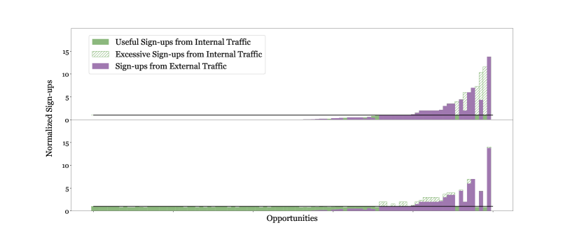
Figure 4: Distribution of sign-ups for each opportunity (normalized by its capacity) as well as the source of sign-ups in one simulation of CP (top) and AC (bottom) on the base instance constructed in Section 6.1.

A simple adjustment of CP that accounts for capacity (i.e., SCP) bridges a large portion of the gap, though AC continues to outperform SCP by 5-10%, depending on the instance. Our other simple heuristic, RC, actually performs the best out of all the considered algorithms in the base instance ($0.984$). However, its performance suffers when compatibility varies over time: in the third instance, AC outperforms RC by 5%.

We conclude this discussion by comparing AC to two other algorithms with strong theoretical guarantees in certain special cases: GPG (which obtains the optimal guarantee when sign-ups are deterministic) and MSVV (which is asymptotically optimal in the absence of external traffic). Potentially because it does not adapt based on the current fill rate of opportunities, GPG performs worse than AC in all three instances, by up to $3.7\%$. In contrast, the performance of AC and MSVV is quite similar, as one might expect given the relatively low EFET. Their relative performance is always within $0.7\%$ across the three instances, with MSVV performing slightly better in all three instances. Due to the similarities in performance between these two algorithms in the constructed instances, we next dig a bit deeper into instance features that drive performance gaps between AC and MSVV.

Figure 5: Relative performance of AC and MSVV (averaged over 10,000 simulations) for two different arrival patterns as a function of the EFET $\beta$. The standard errors are negligible.

6.3 Comparison Between AC and MSVV:

As discussed in Section 4.3 and illustrated in Figure 2(b), the competitive ratio of AC is only strictly better than the competitive ratio of MSVV when the EFET $\beta$ is sufficiently large. In the instances we constructed in Section 6.1, we have $\beta=0.19$. To obtain instances with a larger EFET, we scale up the number of external traffic arrivals while continuing to sample from the view distribution of external traffic to determine their targeted opportunity. This enables us to construct instances where the EFET varies from 0.19 to 0.45. (Even large numbers of external traffic arrivals cannot meaningfully exceed this EFET given our sampling approach, as only 49 of the 100 opportunities in our subset receive any views from external traffic.) To keep the achievable performance as similar as possible in each of these instances, we correspondingly reduce the number of internal traffic arrivals such that our benchmark $\overline{\textnormal{{OPT}}}$ remains the same. We determine compatibility for these internal traffic arrivals using the same procedure described in our base instance.

For a sufficient amount of external traffic, the key factor that separates the performance of AC and MSVV lies in how they account for external traffic in their definition of an opportunity’s fill rate. In particular, AC imposes a weaker penalty than MSVV when capacity is filled by external traffic. Based on this observation, as discussed at the end of Section 4.3, we would expect AC to perform better in instances where opportunities with external traffic should not be harshly penalized (e.g., if opportunities with early-arriving external traffic have fewer compatible arrivals in the future), whereas MSVV should perform better when opportunities with external traffic can safely be penalized (e.g., if some external traffic is predictive of more external traffic in the future).

Fixing an EFET $\beta$, we numerically assess this hypothesis by considering two different modifications of the arrival sequence. First, we consider an arrival sequence where external traffic arrives in bursts. Specifically, building on the intuition developed in our hardness examples for MSVV (see Propositions 2 and 4), we partition the external traffic into two groups. If an external traffic volunteer $t$ targets an opportunity that can be entirely filled with external traffic, then $t$ arrives at the end of the arrival sequence (i.e., after all internal traffic). Otherwise, if $t$ targets an opportunity that can only be partially filled with external traffic, then $t$ arrives at the beginning of the arrival sequence (i.e., before all internal traffic). Roughly speaking, in this arrival sequence, it is better to minimally penalize opportunities for external traffic arrivals; hence, AC should outperform MSVV.

To complement this arrival sequence, we considered an arrival sequence where external traffic is spread out. For this arrival sequence, we assume external traffic arrives in a random order, which means each external traffic arrival is predictive of future external traffic arrivals. Roughly speaking, larger penalties for external traffic should be better in this setting, which means MSVV should perform better than AC.

For each of these modified instances, we simulate both algorithms 10,000 times and we report the results in Figure 5 as a function of the EFET $\beta$. Here, the ratio of AC to MSVV for the arrival sequence where external traffic arrives in bursts (resp. where external traffic is spread out) is shown by the blue line with squares (resp. red line with triangles). Consistent with our intuition, AC does better than MSVV when external traffic arrives in bursts because it appropriately limits the penalty for sign-ups from external traffic, and its relative improvement grows as a function of $\beta$. In contrast, MSVV performs better when external traffic is spread out over time.

This can guide practitioners in determining which algorithm is most suitable for their setting: if external traffic represents a significant portion of traffic and arrives in unpredictable bursts, AC may be preferable due to its superior worst-case performance. However, if external traffic arrives consistently and spread over time, then the platform should either implement MSVV or account for this in the design of AC (i.e., by continuously predicting the amount of future external traffic for each opportunity and reducing capacities accordingly).

7 Conclusion

In this paper, we introduce a framework for making online recommendations to maximize matches in the presence of external traffic, motivated by platforms such as VolunteerMatch (the largest online volunteer engagement network in the US, and our industry partner). Our recommendation algorithm, Adaptive Capacity (AC), does not know the amount of external traffic a priori, yet it nevertheless provides strong parameterized guarantees (relative to both the commonly-used MSVV algorithm and the upper bound we establish on any online algorithm).

Beyond theoretical guarantees, we demonstrate AC’s practical effectiveness in simulations based on VM data. We are currently collaborating with VM to implement a version of our algorithm.

More generally, our work shows the importance of accounting for the source of traffic in decision-making on platforms with multi-channel traffic, which opens up opportunities for further research. For instance, while we have focused on settings where the platform cannot influence external traffic, some platforms may have some degree of control over the timing or the destination of this traffic (e.g., via marketing campaigns or curated email recommendations). Also, platforms with external traffic may have objectives beyond maximizing the number of matches (e.g., platforms such as DonorsChoose may aim to maximize the number of donation campaigns that reach a certain threshold). Studying the platform design in such settings is an interesting direction for future work.

8 Omitted Proofs of Section 4

We first present the proofs of the three theorems from Section 4, in order of their appearance in the text. We then proceed to the proofs of the propositions, also in order of appearance.

8.1 Proof of Theorem 1 (Section 4.2)

This proof is an adaptation of the proof of Theorem 7.1 in Mehta et al. [2007], which we have generalized to apply in our setting. We aim to prove that no online algorithm (deterministic or randomized) can provide a competitive ratio greater than $\big{(}1-1/e\big{)}\mathbbm{1}_{\beta\leq 1/e}+\big{(}1+\beta\log(\beta)\big{)}\mathbbm{1}_{\beta>1/e}$. By Yao’s Lemma [Yao, 1977], it is sufficient to show that there exists a distribution over a set of instances for which no deterministic algorithm can provide an expected value greater than $\Big{(}\big{(}1-1/e\big{)}\mathbbm{1}_{\beta\leq 1/e}+\big{(}1+\beta\log(\beta)\big{)}\mathbbm{1}_{\beta>1/e}\Big{)}\textnormal{{OPT}}$.

We begin by fixing an EFET $\beta$ and describing an instance $\mathcal{I}_{1}(\beta)$. In this instance, the set of opportunities is of size $N$, each with identical large capacity $C$. The arrival sequence consists of $NC$ volunteers. The first $(1-\beta)NC$ of these volunteers are internal traffic, and the remaining $\beta NC$ are external traffic. All volunteers have conversion probabilities of $1$ or $0$, and if $\mu_{i,t}=1$ (resp. 0), we will refer to opportunity $i$ and volunteer $t$ as compatible (resp. incompatible).

The arrival sequence of $\mathcal{I}_{1}(\beta)$ can be broken down into $N$ batches of $C$ sequentially-arriving identical volunteers. For each $j\in\{1,\ldots,(1-\beta)N\}$, the $j$^th batch of volunteers consists of internal traffic that is compatible with all opportunities $i\geq j$. For each $j\in\{(1-\beta)N+1,\ldots,N\}$, the $j$^th batch of volunteers consists of external traffic which views (and is compatible with) opportunity $i^{*}_{j}=j$. This external traffic can fill the entire capacity of each of these $\beta N$ opportunities, which implies that the EFET is equal to $\beta$ in such an instance.

We first establish the value of OPT on instance $\mathcal{I}_{1}(\beta)$.

Claim 1

For any EFET $\beta$, OPT achieves a value of $NC$ on $\mathcal{I}_{1}(\beta)$.

Proof.

Proof of Claim 1: Consider a solution which matches each of the $C$ volunteers in the $j$^th batch to opportunity $j$, for all $j\in[N]$. These volunteer-opportunity pairs are all compatible based on the compatibility structure previously described, and (since the conversion probabilities are exactly equal to $1$) each opportunity will exactly reach its capacity of $C$. As this solution fills all capacity, OPT must also fill all capacity, thereby achieving a total value of $NC$, regardless of the EFET $\beta$. ∎

We now consider the set of instances which can be obtained from $\mathcal{I}_{1}(\beta)$ by permuting the indices of the opportunities. Specifically, we apply a permutation $\mathcal{P}$ to the set of opportunities such that any algorithm sees opportunities with indices $\{\mathcal{P}(1),\ldots,\mathcal{P}(N)\}$. We highlight that a priori the opportunities appear identical to an online algorithm, aside from their indices. We augment our previous notation and describe such an instance as $\mathcal{I}_{1}(\beta,\mathcal{P})$.

Suppose that the permutation $\mathcal{P}$ is drawn uniformly at random from the set of all permutations of $N$ indices. For the set of instances generated by this distribution over permutations, in the following lemma, we place an upper-bound on the expected value of any deterministic online algorithm.

Claim 2

Consider any deterministic online algorithm $\pi$. For any EFET $\beta$,

$$\mathbb{E}_{\mathcal{P}}[\pi(\mathcal{I}_{1}(\beta,\mathcal{P}))]\leq\sum_{i\in[(1-\beta)N]}\min\left\{C,\sum_{j=1}^{i}\frac{C}{N-j+1}\right\}+\sum_{i\in[N]\setminus[(1-\beta)N]}C,$$ (12)

where the expectation is taken with respect to the uniform distribution over permutations $\mathcal{P}$.

Proof.

Proof of Claim 2: To aid in this proof, let us define $d_{i,j}$ as the amount of volunteers allocated to opportunity $i$ from the $j$^th batch of arriving volunteers. Recall that for $j\in\{1,\ldots,(1-\beta)N\}$, volunteers in the $j$^th batch of arrivals are compatible with all opportunities $i\geq j$. Thus, we have:

$$E_{\mathcal{P}}[d_{i,j}]\leq\begin{dcases}\frac{C}{N-j+1},&\text{if }i\geq j\\ 0&\text{if }i<j\end{dcases}$$

To see why this must be the case, note that for each volunteer in the $j$^th batch of volunteers, there are a total of $N-j+1$ compatible opportunities. The online algorithm cannot distinguish between these compatible opportunities, as it only observes the indices $\{\mathcal{P}(j),\ldots,\mathcal{P}(N)\}$. Specifically, if $i$ is one such compatible opportunity, the online algorithm does not know which index in the set $\{\mathcal{P}(j),\ldots,\mathcal{P}(N)\}$ is equal to $\mathcal{P}(i)$. Hence, the expected amount of volunteers allocated to opportunity $i$ cannot exceed $\frac{C}{N-j+1}$, when taking expectation with respect to the uniform distribution over permutations $\mathcal{P}$.

More simply, for batches $j\in\{(1-\beta)N+1,N\}$, the volunteers are only compatible with opportunity $i$ if $i=j$. Hence,

$$E_{\mathcal{P}}[d_{i,j}]\leq\begin{dcases}C&\text{if }i=j\\ 0&\text{if }i\neq j\end{dcases}$$

After the arrival of all volunteers, the expected fill of opportunity $i$ is upper-bounded by $\sum_{j\in[N]}E_{\mathcal{P}}[d_{i,j}]$. This quantity is either $C$ (if $i>(1-\beta)N$) or $\min\{C,\sum_{j=1}^{i}\frac{C}{N-j+1}\}$ (if $i\leq(1-\beta)N$). Summing over all opportunities, we have the following upper bound on the value of any online algorithm:

$$\sum_{i\in[(1-\beta)N]}\min\left\{C,\sum_{j=1}^{i}\frac{C}{N-j+1}\right\}+\sum_{i\in[N]\setminus[(1-\beta)N]}C$$ (13)

This completes the proof of Claim 2.∎

Together, and in combination with Yao’s lemma, these claims establish an upper-bound on the achievable competitive ratio of any online algorithm of

$$\frac{1}{NC}\left(\sum_{i\in[(1-\beta)N]}\min\left\{C,\sum_{j=1}^{i}\frac{C}{N-j+1}\right\}+\sum_{i\in[N]\setminus[(1-\beta)N]}C\right)\quad\rightarrow\quad\big{(}1-1/e\big{)}\mathbbm{1}_{\beta\leq 1/e}+\big{(}1+\beta\log(\beta)\big{)}\mathbbm{1}_{\beta>1/e},$$ (14)

where the limit holds as $C$ and $N$ approach infinity.

8.2 Proof of Theorem 2 (Section 4.2)

The proof builds on proof ideas in Mehta et al. [2007], with additional intricacies to account for external traffic. As in Mehta et al. [2007], our analysis relies on a partition of opportunities into a sufficiently large number of types, where an opportunity’s type is determined by its fill rate after a run of our algorithm. We begin by presenting the outline of our proof; we then present the omitted proofs of intermediate results in Appendices 8.2.1 through 8.2.4.

Recall that the fill rate of opportunity $u$ under AC at the end of the arrival sequence is given by $\textsc{FR}_{u,T}=\textnormal{{AC}}_{u,T}^{\textsc{int}}/(c_{u}-\textnormal{{AC}}_{u,T}^{\textsc{ext}})$. This fill rate definition represents a crucial difference between AC and MSVV, and our analysis relies on AC’s fill rate definition to establish an improved competitive ratio. Fixing $k\in\mathbb{N}$ (we will think of $k$ as a large number), an opportunity $u$ belongs to type $i$ if its fill rate under AC at the end of the arrival sequence is in the interval $[(i-1)/k,i/k)$.

Notation:

Throughout the proof, we will fix an instance and we fix the number of opportunity types $k$, where we assume $k\geq 4\underline{c}/\beta$. Let $O_{i}$ denote the set of opportunities of type $i$. We will use $n_{i}$ to denote the aggregate capacity of type $i$ opportunities (i.e., $n_{i}=\sum_{u\in O_{i}}c_{u}$), and the total capacity is given by $N=\sum_{i=1}^{k}n_{i}$. We will use $b_{i}$ to denote the total capacity of type $i$ opportunities that can be filled by external traffic, which implies that $\sum_{i=1}^{k}b_{i}=\beta N$ based on our definition of the EFET. Furthermore, let $a_{j}$ denote the total capacity of type $j$ opportunities that OPT fills with internal traffic.

Using the partition of opportunities into types, we prove Theorem 2 in four steps. (i) First, in Lemma 3, we lower-bound the value of AC as a function of $n_{i}$ and $b_{i}$. (ii) Then, in Lemma 4, we introduce an important constraint that relates the performance of OPT to the value of each $n_{i}$. (iii) We combine these two lemmas with other natural constraints to formulate an LP that lower-bounds the value of AC, as formally established in Lemma 5. (iv) We conclude in Lemma 6 by establishing that the value of this LP is at least $\textnormal{{OPT}}\bigg{(}\big{(}1-1/e\big{)}\mathbbm{1}_{\beta\leq 1/e}+\big{(}1+\beta\log(\beta)\big{)}\mathbbm{1}_{\beta>1/e}-2/\underline{c}\bigg{)}$.

Lemma 3

The value of AC is at least

$$\sum_{i=1}^{k}\Big{(}\frac{i}{k}n_{i}+\frac{k-i}{k}b_{i}\Big{)}-\frac{1}{k}N$$ (15)

The proof of Lemma 3 is algebraic and follows from the fact that $\textnormal{{AC}}_{u,T}^{\textsc{int}}/(c_{u}-\textnormal{{AC}}_{u,T}^{\textsc{ext}})\geq(i-1)/k$ for any opportunity of type $i$, based on AC’s fill rate definition. We formally prove Lemma 3 in Appendix 8.2.1.

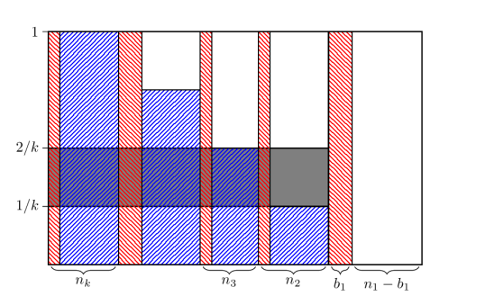
Figure 6: Visualization of the outcome of AC where opportunities are grouped by type. The area of red down-sloping rectangles represent the capacity that can be filled by external traffic, and the area of the blue up-sloping rectangles is a lower bound on the capacity filled by internal traffic under AC. The shaded region corresponds to an upper bound on the total capacity in slab 2 filled under AC.

We can also establish this result via a proof-by-picture, using Figure 6 as our visual aid. The overall length of Figure 6 is equal to the total capacity $N$, and we organize the opportunities from right to left in increasing order of their type. Each type $i\in\{1,\dots,k\}$ corresponds to a segment of length $n_{i}$ (i.e., the total capacity of opportunities of type $i$). Within each segment, there are two rectangles, one filled with red down-sloping diagonals and another filled with blue up-sloping diagonals. The former rectangles have width $b_{i}$ and height $1$; their area represents the total amount of capacity of type $i$ opportunities that can filled by external traffic. The latter rectangles have width $n_{i}-b_{i}$ and height $(i-1)/k$; their area represents a lower bound on the total amount of capacity of type $i$ opportunities that AC fills with internal traffic. Due to the fact that AC uses all external traffic for an opportunity unless the opportunity is full, the total area of the red and blue rectangles represents a lower bound on the value of AC. This total area is equivalent to the bound in Lemma 3. We next relate this area to the value of OPT.

Lemma 4

Let $a_{j}$ denote the total capacity of type $j$ opportunities that OPT fills with internal traffic. Then for all $i\in\{1,\dots,k-1\}$,

$$\sum_{j=1}^{i}a_{j}\quad\leq\quad\frac{i}{k}N-\sum_{j=1}^{i}\frac{i-j}{k}n_{j}+\sum_{j=i+1}^{k}\frac{1}{\underline{c}}n_{j}$$ (16)

We formally prove Lemma 4 in Appendix 8.2.2, but the proof idea can likewise be visualized in Figure 6. To see this, suppose we discretize each opportunity’s capacity into $k$ equally sized slabs, numbered from $1$ to $k$, where slab $j$ consists of the $(j-1)/k$ to $j/k$ percentile of each opportunity’s capacity. Based on AC’s optimality condition, in a setting with unweighted deterministic rewards, every internal traffic arrival $t$ assigned by OPT to opportunities of type (at most) $i$ must fill capacity in slab $j\leq i$ under AC. (Such an assignment can span multiple slabs, which we rigorously account for in the formal proof of Lemma 16.) We emphasize that this crucial observation no longer holds when rewards are weighted: in that case, an assignment by OPT to an opportunity of type (at most) $i$ may fill (less) capacity in slab $j>i$ under AC. This highlights the difficulty of extending such a result to settings with weighted rewards.

Note that under AC, opportunities with type at most $i$ have a fill rate of at most $i/k$. Hence, for these opportunities, we know that capacity in slab $j>i$ is not filled by internal traffic (e.g., capacity in slab 2 is not filled by internal traffic under AC for opportunities of type 1). In Figure 6, we use a shaded rectangle to represent an upper bound on the total capacity in slab 2 filled under AC. The total capacity of slabs $j\leq i$ filled by AC is upper-bounded by the first two terms in Equation (16). The final term in the upper bound incorporates the minimum capacity to account for the fact that a sign-up can span multiple slabs when capacities are small.

Based on Lemmas 3 and 4 as well as other natural constraints, we introduce an instance-specific LP whose solution serves as a lower bound on the value of AC, as established in Lemma 5.

$$\begin{array}[]{|llll|}\hline\cr&&&\\ \min_{\mathbf{a_{,}b_{,}n_{missing}}}&\displaystyle\sum_{i=1}^{k}\Big{(}\frac{i}{k}n_{i}+\frac{k-i}{k}b_{i}\Big{)}-\frac{1}{k}N&&(\textsc{LP})\\[11.19997pt] \text{s.t.}&\displaystyle\sum_{j=1}^{i}a_{j}\quad\leq\quad\frac{i}{k}N-\sum_{j=1}^{i}\frac{i-j}{k}n_{j}+\sum_{j=i+1}^{k}\frac{1}{\underline{c}}n_{j}&i\leq k-1&(\alpha_{i})\\[14.40004pt] &\displaystyle b_{i}+a_{i}\quad\leq\quad n_{i}&i\leq k&(\gamma_{i})\\[8.00002pt] &\displaystyle\beta N\quad\leq\quad\sum_{i=1}^{k}n_{i}&&({\color[rgb]{0,0,0}\lambda})\\[11.19997pt] &\displaystyle\textnormal{{OPT}}\quad\leq\quad\beta N+\sum_{i=1}^{k}a_{i}&&({\color[rgb]{0,0,0}\theta})\\[11.19997pt] &\displaystyle N\quad\leq\quad\sum_{i=1}^{k}n_{i}&&({\color[rgb]{0,0,0}\mu})\\[11.19997pt] \hline\cr\end{array}$$

Lemma 5

For any problem instance, the value of LP is a lower bound on the value of AC on that instance.

We prove Lemma 5 in Appendix 8.2.3. Based on this lemma, to establish a bound on the competitive ratio of AC it suffices to bound the value of LP, which we do in the following lemma.

Lemma 6

The value of LP is at least $\textnormal{{OPT}}\Big{(}\big{(}1-1/e\big{)}\mathbbm{1}_{\beta\leq 1/e}+\big{(}1+\beta\log(\beta)\big{)}\mathbbm{1}_{\beta>1/e}-2/\underline{c}\Big{)}$.

To prove Lemma 6, we find a feasible solution to the dual of LP which obtains a value of $\textnormal{{OPT}}\Big{(}\big{(}1-1/e\big{)}\mathbbm{1}_{\beta\leq 1/e}+\big{(}1+\beta\log(\beta)\big{)}\mathbbm{1}_{\beta>1/e}-2/\underline{c}\Big{)}$. We provide the full details in Appendix 8.2.1. Because the value of LP provides a lower bound on the value of AC for any problem instance (by Lemma 5), it immediately follows from Lemma 6 that the competitive ratio of AC is lower-bounded by $\big{(}1-1/e\big{)}\mathbbm{1}_{\beta\leq 1/e}+\big{(}1+\beta\log(\beta)\big{)}\mathbbm{1}_{\beta>1/e}-2/\underline{c}$. This completes the proof of Theorem 2.

8.2.1 Proof of Lemma 3

Let $O_{i}$ denote the set of opportunities of type $i$. By definition, for all $u\in O_{i}$ we have $\textnormal{{AC}}_{u,T}^{\textsc{int}}/(c_{u}-\textnormal{{AC}}_{u,T}^{\textsc{ext}})\geq(i-1)/k$. This implies $\textnormal{{AC}}_{u,T}^{\textsc{int}}\geq(c_{u}-\textnormal{{AC}}_{u,T}^{\textsc{ext}})\cdot(i-1)/k$.

We now aggregate the total filled capacity for each opportunity under AC:

AC $$=\sum_{i=1}^{k}\sum_{u\in O_{i}}\textnormal{{AC}}_{u,T}^{\textsc{int}}+\textnormal{{AC}}_{u,T}^{\textsc{ext}}$$

$$\geq\sum_{i=1}^{k}\sum_{u\in O_{i}}\frac{i-1}{k}(c_{u}-\textnormal{{AC}}_{u,T}^{\textsc{ext}})+\textnormal{{AC}}_{u,T}^{\textsc{ext}}$$

$$=\sum_{i=1}^{k}\sum_{u\in O_{i}}\frac{i-1}{k}c_{u}+\frac{k-i+1}{k}\textnormal{{AC}}_{u,T}^{\textsc{ext}}$$

$$\geq\sum_{i=1}^{k}\sum_{u\in O_{i}}\frac{i-1}{k}c_{u}+\frac{k-i}{k}\textnormal{{AC}}_{u,T}^{\textsc{ext}}$$

$$=\sum_{i=1}^{k}\frac{i-1}{k}n_{i}+\frac{k-i}{k}b_{i}$$

To see why the final step holds with equality, note that the first terms are identical by definition of $n_{i}$. For the second term, if $u$ is not of type $k$ (i.e., if the opportunity has remaining capacity after a run of AC), then AC must use all external traffic for $u$. In that case, $\sum_{u\in O_{i}}\textnormal{{AC}}_{u,T}^{\textsc{ext}}=b_{i}$ by the definition of $b_{i}$. If $u$ is of type $k$, then AC may not use all external traffic for $u$; however, the coefficient is $0$.

8.2.2 Proof of Lemma 4

Suppose OPT uses internal traffic arrival $t$ to fill one unit of capacity of $v\in O_{i}$. We want to understand what AC did with that arrival. If $i<k$, then there must have been at least one compatible opportunity for $t$ under AC that had capacity left, and hence it must have been matched. Suppose it was matched to $u$. The definition of AC ensures that $u\in\text{argmin}_{u^{\prime}}\textnormal{{AC}}_{u^{\prime},t-1}^{\textsc{int}}/(c_{u^{\prime}}-\textnormal{{AC}}_{u^{\prime},t-1}^{\textsc{ext}})$. Based on this optimality condition and the fact that this fill rate is non-decreasing in $t$ and $v\in O_{i}$,

$$\frac{\textnormal{{AC}}_{u,t-1}^{\textsc{int}}}{c_{u}-\textnormal{{AC}}_{u,t-1}^{\textsc{ext}}}\quad\leq\quad\frac{\textnormal{{AC}}_{v,t-1}^{\textsc{int}}}{c_{v}-\textnormal{{AC}}_{v,t-1}^{\textsc{ext}}}\quad\leq\quad\frac{\textnormal{{AC}}_{v,T}^{\textsc{int}}}{c_{v}-\textnormal{{AC}}_{v,T}^{\textsc{ext}}}\quad\leq\quad\frac{i}{k}$$ (17)

In other words, every time OPT assigns an internal arrival to an opportunity of type $i$ (where $i\leq k$), AC must assign that arrival to an opportunity with a bounded amount of internal traffic. How many of these assignments can AC make?

Suppose the opportunity $u$ that this internal traffic is matched with under AC is of type $j$, i.s., $u\in O_{j}$. Then,

$$\frac{\textnormal{{AC}}_{u,t-1}^{\textsc{int}}}{c_{u}-\textnormal{{AC}}_{u,t-1}^{\textsc{ext}}}\quad\leq\quad\frac{\textnormal{{AC}}_{u,T}^{\textsc{int}}}{c_{u}-\textnormal{{AC}}_{u,T}^{\textsc{ext}}}\quad\leq\quad\frac{j}{k}$$ (18)

If $j\leq i$, then $u$ receives at most $(j/k)c_{u}$ sign-ups from internal traffic under AC (based on equation (18)). Otherwise, AC may only assign this arrival to $u$ if $\textnormal{{AC}}_{u,t-1}^{\textsc{int}}\leq\frac{i}{k}c_{u}$ (based on Equation (17)), so there can be at most $\frac{i}{k}c_{u}+1$ such assignments.

Putting these facts together, we can bound the total amount of internal traffic that OPT assigns to opportunities of type $1$:

$$\sum_{v\in O_{1}}\textnormal{{OPT}}_{v,T}^{\textsc{int}}\quad\leq\quad\sum_{u\in O_{1}}\frac{1}{k}c_{u}+\sum_{j=2}^{k}\sum_{u\in O_{j}}\left(\frac{1}{k}c_{u}+1\right)$$

By the same logic, we can bound the total amount of internal traffic that OPT assigns to opportunities with type at most $i$:

$$\sum_{j=1}^{i}\sum_{v\in O_{j}}\textnormal{{OPT}}_{v,T}^{\textsc{int}}\quad\leq\quad\sum_{j=1}^{i}\sum_{u\in O_{j}}\frac{j}{k}c_{u}+\sum_{j=i+1}^{k}\sum_{u\in O_{j}}\left(\frac{i}{k}c_{u}+1\right)$$

We now re-write this bound, recalling that $a_{j}$ denotes the total capacity of type $j$ opportunities that OPT fills with internal traffic, and that $n_{j}$ denotes the total capacity of type $j$ opportunities.

$$\sum_{j=1}^{i}a_{j}\quad \leq\quad\sum_{j=1}^{i}\frac{j}{k}n_{j}+\sum_{j=i+1}^{k}\frac{i}{k}n_{j}+\sum_{j=i+1}^{k}\sum_{u\in O_{j}}\frac{c_{u}}{c_{u}}$$

$$\leq\quad\sum_{j=1}^{i}\Big{(}\frac{i}{k}-\frac{i-j}{k}\Big{)}n_{j}+\sum_{j=i+1}^{k}\frac{i}{k}n_{j}+\sum_{j=i+1}^{k}\sum_{u\in O_{j}}\frac{c_{u}}{\underline{c}}$$

$$\leq\quad\frac{i}{k}N-\sum_{j=1}^{i}\frac{i-j}{k}n_{j}+\sum_{j=i+1}^{k}\frac{1}{\underline{c}}n_{j}$$

The first inequality follows by the definition of $n_{j}$, i.e., $n_{j}=\sum_{u\in O_{j}}c_{u}$, and the last inequality follows by the definition of $N$, i.e., $N=\sum_{j=1}^{k}n_{j}$. This completes the proof of Lemma 4.

8.2.3 Proof of Lemma 5

We reproduce LP here for ease of reference. By Lemma 4, the first set of constraints must hold. The second set of constraints holds because OPT cannot fill an opportunity beyond its capacity. The third constraint holds by definition of the EFET $\beta$ (see Definition 2). The fourth constraint holds because OPT cannot use more external traffic than what exists. The final constraint holds because the sum of capacities across all types is equal to the total capacity.

$$\begin{array}[]{|llll|}\hline\cr&&&\\ \min_{\mathbf{a_{,}b_{,}n_{missing}}}&\displaystyle\sum_{i=1}^{k}\Big{(}\frac{i}{k}n_{i}+\frac{k-i}{k}b_{i}\Big{)}-\frac{1}{k}N&&(\textsc{LP})\\[11.19997pt] \text{s.t.}&\displaystyle\sum_{j=1}^{i}a_{j}\quad\leq\quad\frac{i}{k}N-\sum_{j=1}^{i}\frac{i-j}{k}n_{j}+\sum_{j=i+1}^{k}\frac{1}{\underline{c}}n_{j}&i\leq k-1&(\alpha_{i})\\[14.40004pt] &\displaystyle b_{i}+a_{i}\quad\leq\quad n_{i}&i\leq k&(\gamma_{i})\\[8.00002pt] &\displaystyle\beta N\quad\leq\quad\sum_{i=1}^{k}n_{i}&&({\color[rgb]{0,0,0}\lambda})\\[11.19997pt] &\displaystyle\textnormal{{OPT}}\quad\leq\quad\beta N+\sum_{i=1}^{k}a_{i}&&({\color[rgb]{0,0,0}\theta})\\[11.19997pt] &\displaystyle N\quad\leq\quad\sum_{i=1}^{k}n_{i}&&({\color[rgb]{0,0,0}\mu})\\[11.19997pt] \hline\cr\end{array}$$

8.2.4 Proof of Lemma 6

To prove Lemma 6, it is sufficient to find a feasible solution to the dual of LP (reproduced above) which obtains a value of at least $\textnormal{{OPT}}\Big{(}\big{(}1-1/e\big{)}\mathbbm{1}_{\beta\leq 1/e}+\big{(}1+\beta\log(\beta)\big{)}\mathbbm{1}_{\beta>1/e}-2/\underline{c}\Big{)}$. For now, we will assume that $\underline{c}\geq 3$. At the end of the proof, we will briefly revisit the case where $\underline{c}<3$ and show that the lemma holds. We present the dual of LP below.

The dual of LP.

$$\begin{array}[]{llll}\max_{\mathbf{\alpha,\gamma},{\color[rgb]{0,0,0}\lambda},{\color[rgb]{0,0,0}\theta},{\color[rgb]{0,0,0}\mu}}&\displaystyle{\color[rgb]{0,0,0}\theta}\textnormal{{OPT}}+({\color[rgb]{0,0,0}\lambda}-{\color[rgb]{0,0,0}\theta})\beta N+{\color[rgb]{0,0,0}\mu}N-\sum_{j=1}^{k-1}\Big{(}\frac{j}{k}\alpha_{j}N\Big{)}-\frac{1}{k}N&&(\textsc{DUAL})\\[13.99995pt] \text{s.t.}&\displaystyle 0\quad\leq\quad\gamma_{i}-{\color[rgb]{0,0,0}\lambda}+\frac{k-i}{k}&i\leq k&(b_{i})\\[13.99995pt] &\displaystyle 0\quad\leq\quad\frac{i}{k}-\gamma_{i}-{\color[rgb]{0,0,0}\mu}+\sum_{j=i}^{k-1}\Big{(}\frac{j-i}{k}\Big{)}\alpha_{j}-\sum_{j=k-i+1}^{k-1}\Big{(}\frac{1}{\underline{c}}\Big{)}\alpha_{j}&i\leq k&(n_{i})\\[13.99995pt] &\displaystyle 0\quad\leq\quad\gamma_{i}-{\color[rgb]{0,0,0}\theta}+\sum_{j=i}^{k-1}\alpha_{j}&i\leq k&(a_{i})\\[13.99995pt] \end{array}$$

Candidate solution.

Our candidate solution, presented below, will depend on the EFET $\beta$ via an index $\hat{i}:=\min\{k-1,\lfloor-k\log(\beta)\rfloor\}$.

$$\alpha_{i}\quad =\quad\begin{cases}\frac{\Big{(}1+\frac{1}{k}\Big{)}^{i}}{k\Big{(}1+\frac{1}{k}\Big{)}^{\hat{i}+1}},&i\leq\hat{i}\\ 0,&i>\hat{i}\end{cases}$$ (19)

$$\gamma_{i}\quad =\quad\frac{i}{k}\Big{(}1-\sum_{j=i}^{k-1}\alpha_{j}\Big{)}-\sum_{j=1}^{i-1}\Big{(}\frac{j}{k}\Big{)}\alpha_{j}-\sum_{j=k-i+1}^{k-1}\Big{(}\frac{1}{\underline{c}}\Big{)}\alpha_{j}$$ (20)

$${\color[rgb]{0,0,0}\lambda}\quad =\quad 1-\sum_{j=1}^{k-1}\Big{(}\frac{j}{k}+\frac{1}{\underline{c}}\Big{)}\alpha_{j}$$ (21)

$${\color[rgb]{0,0,0}\mu}\quad =\quad\sum_{j=1}^{k-1}\Big{(}\frac{j}{k}\Big{)}\alpha_{j}$$ (22)

$${\color[rgb]{0,0,0}\theta}\quad =\quad\sum_{j=1}^{k-1}\Big{(}1-\frac{1}{\underline{c}}\Big{)}\alpha_{j}$$ (23)

We prove Lemma 6 in three steps: (i) we show that this candidate solution satisfies the three dual constraints, (ii) we show that the dual variables are non-negative, and (iii) we bound the objective value of this candidate solution.

In these three steps, we will leverage the following two properties of the $\alpha_{i}$ terms.

$$\sum_{j=i}^{k-1}\alpha_{j}\quad =\quad\begin{cases}1-\frac{\Big{(}1+\frac{1}{k}\Big{)}^{i}}{\Big{(}1+\frac{1}{k}\Big{)}^{\hat{i}+1}},&i\leq\hat{i}\\ 0,&i>\hat{i}\end{cases}$$ (24)

$$\sum_{j=1}^{i-1}\Big{(}\frac{k+j}{k}\Big{)}\alpha_{j}\quad =\quad\begin{cases}\Big{(}\frac{i-1}{k}\Big{)}\frac{\Big{(}1+\frac{1}{k}\Big{)}^{i}}{\Big{(}1+\frac{1}{k}\Big{)}^{\hat{i}+1}},&i\leq\hat{i}\\ \hat{i}/k,&i>\hat{i}\end{cases}$$ (25)

To establish the first property, we use the fact that for any $m\in\mathbb{N}$, $\sum_{j=i}^{m}r^{j}=\frac{r^{m+1}-r^{\min\{i,m+1\}}}{r-1}$:

$$\sum_{j=i}^{k-1}\alpha_{j}\quad =\quad\left(\frac{1}{k\Big{(}1+\frac{1}{k}\Big{)}^{\hat{i}+1}}\right)\sum_{j=i}^{\hat{i}}\Big{(}1+\frac{1}{k}\Big{)}^{j}$$

$$=\quad\left(\frac{1}{k\Big{(}1+\frac{1}{k}\Big{)}^{\hat{i}+1}}\right)\frac{\Big{(}1+\frac{1}{k}\Big{)}^{\hat{i}+1}-\Big{(}1+\frac{1}{k}\Big{)}^{\min\{i,\hat{i}+1\}}}{\Big{(}1+\frac{1}{k}\Big{)}-1}$$

$$=\quad\begin{cases}1-\frac{\Big{(}1+\frac{1}{k}\Big{)}^{i}}{\Big{(}1+\frac{1}{k}\Big{)}^{\hat{i}+1}},&i\leq\hat{i}\\ 0,&i>\hat{i}\end{cases}$$

The second property also uses the fact that for any $m\in\mathbb{N}\cup\{0\}$, $\sum_{j=1}^{m}j\cdot r^{j}=\frac{m\cdot r^{m+2}-(m+1)r^{m+1}+r}{(r-1)^{2}}$. For now, let us assume that $i\leq\hat{i}+1$, thereby ensuring that each term in the summation is strictly positive.

$$\sum_{j=1}^{i-1}\Big{(}\frac{k+j}{k}\Big{)}\alpha_{j}\quad =\quad\left(\frac{1}{k\Big{(}1+\frac{1}{k}\Big{)}^{\hat{i}+1}}\right)\sum_{j=1}^{i-1}\Big{(}1+\frac{j}{k}\Big{)}\Big{(}1+\frac{1}{k}\Big{)}^{j}$$

$$=\quad\left(\frac{1}{k\Big{(}1+\frac{1}{k}\Big{)}^{\hat{i}+1}}\right)\left(\frac{\Big{(}1+\frac{1}{k}\Big{)}^{i}-\Big{(}1+\frac{1}{k}\Big{)}}{\Big{(}1+\frac{1}{k}\Big{)}-1}\right.$$

$$\qquad\qquad\left.+\frac{1}{k}\Bigg{(}\frac{(i-1)\big{(}1+\frac{1}{k}\big{)}^{i+1}-i\cdot\big{(}1+\frac{1}{k}\big{)}^{i}+\big{(}1+\frac{1}{k}\big{)}}{\Big{(}\big{(}1+\frac{1}{k}\big{)}-1\Big{)}^{2}}\Bigg{)}\right)$$

$$=\quad\left(\frac{1}{k\Big{(}1+\frac{1}{k}\Big{)}^{\hat{i}+1}}\right)\left(\frac{(i-1)\Big{(}1+\frac{1}{k}\Big{)}^{i+1}-(i-1)\Big{(}1+\frac{1}{k}\Big{)}^{i}}{1/k}\right)$$

$$=\quad\Big{(}\frac{i-1}{k}\Big{)}\frac{\Big{(}1+\frac{1}{k}\Big{)}^{i}}{\Big{(}1+\frac{1}{k}\Big{)}^{\hat{i}+1}}$$

This corresponds to the first case of Equation (25). If $i>\hat{i}+1$, all additional terms in the summation are $0$; hence the value of the summation remains constant and equal to the case where $i=\hat{i}+1$, which is captured by the second case of Equation (25)

Step (i): The candidate solution satisfies constraints $(b_{i})$, $(n_{i})$, and $(a_{i})$

We begin with the first set of constraints, corresponding to $b_{i}$:

$$\gamma_{i}-{\color[rgb]{0,0,0}\lambda}+\frac{k-i}{k}\quad =\quad\frac{i}{k}\Big{(}1-\sum_{j=i}^{k-1}\alpha_{j}\Big{)}-\sum_{j=1}^{i-1}\Big{(}\frac{j}{k}\Big{)}\alpha_{j}-\sum_{j=k-i+1}^{k-1}\frac{1}{\underline{c}}\alpha_{j}-{\color[rgb]{0,0,0}\Big{(}1-\sum_{j=1}^{k-1}\Big{(}\frac{j}{k}+\frac{1}{\underline{c}}\Big{)}\alpha_{i}\Big{)}}+\frac{k-i}{k}$$

$$\geq\quad{\color[rgb]{0,0,0}\sum_{j=1}^{k-1}\Big{(}\frac{j}{k}\Big{)}\alpha_{j}}-\sum_{j=i}^{k-1}\Big{(}\frac{i}{k}\Big{)}\alpha_{j}-\sum_{j=1}^{i-1}\Big{(}\frac{j}{k}\Big{)}\alpha_{j}$$

$$=\quad\sum_{j=i}^{k-1}\Big{(}\frac{j-i}{k}\Big{)}\alpha_{j}\quad\geq\quad 0$$ (26)

For the second set of constraints, corresponding to $n_{i}$:

$$\frac{i}{k}-\gamma_{i}-{\color[rgb]{0,0,0}\mu}+\sum_{j=i}^{k-1}\Big{(}\frac{j-i}{k}\Big{)}\alpha_{j} -\sum_{j=k-i+1}^{k-1}\Big{(}\frac{1}{\underline{c}}\Big{)}\alpha_{j}$$

$$=\quad\frac{i}{k}-\Big{(}\frac{i}{k}\Big{(}1-\sum_{j=i}^{k-1}\alpha_{j}\Big{)}-\sum_{j=1}^{i-1}\Big{(}\frac{j}{k}\Big{)}\alpha_{j}-\sum_{j=k-i+1}^{k-1}\Big{(}\frac{1}{\underline{c}}\Big{)}\alpha_{j}\Big{)}$$

$$\qquad-{\color[rgb]{0,0,0}\sum_{j=1}^{k-1}\Big{(}\frac{j}{k}\Big{)}\alpha_{j}}+\sum_{j=i}^{k-1}\Big{(}\frac{j-i}{k}\Big{)}\alpha_{j}-\sum_{j=k-i+1}^{k-1}\Big{(}\frac{1}{\underline{c}}\Big{)}\alpha_{j}$$

$$=\quad\sum_{j=i}^{k-1}\Big{(}\frac{i}{k}\Big{)}\alpha_{j}+\sum_{j=1}^{i-1}\Big{(}\frac{j}{k}\Big{)}\alpha_{j}-{\color[rgb]{0,0,0}\sum_{j=1}^{k-1}\Big{(}\frac{j}{k}\Big{)}\alpha_{j}}+\sum_{j=i}^{k-1}\Big{(}\frac{j-i}{k}\Big{)}\alpha_{j}$$

$$=\quad 0$$ (27)

For the third set of constraints, corresponding to $a_{i}$:

$$\gamma_{i}-{\color[rgb]{0,0,0}\theta}+\sum_{j=i}^{k-1}\alpha_{j}\quad =\quad\frac{i}{k}\Big{(}1-\sum_{j=i}^{k-1}\alpha_{j}\Big{)}-\sum_{j=1}^{i-1}\Big{(}\frac{j}{k}\Big{)}\alpha_{j}-\sum_{j=k-i+1}^{k-1}\frac{1}{\underline{c}}\alpha_{j}-{\color[rgb]{0,0,0}\sum_{j=1}^{k-1}\Big{(}1-\frac{1}{\underline{c}}\Big{)}\alpha_{j}}+\sum_{j=i}^{k-1}\alpha_{j}$$

$$\geq\quad\frac{i}{k}\Big{(}1-\sum_{j=i}^{k-1}\alpha_{j}\Big{)}-\sum_{j=1}^{i-1}\Big{(}{\color[rgb]{0,0,0}1}+\frac{j}{k}\Big{)}\alpha_{j}$$

$$=\quad\begin{cases}\Big{(}\frac{1}{k}\Big{)}\frac{\Big{(}1+\frac{1}{k}\Big{)}^{i}}{\Big{(}1+\frac{1}{k}\Big{)}^{\hat{i}+1}},&i\leq\hat{i}\\ \frac{i-\hat{i}}{k},&i>\hat{i}\end{cases}$$ (28)

The final step follows by applying the two properties of $\alpha$ given in Equations (24) and (25). In either case, the value is positive, hence the constraint holds.

Step (ii): Verifying the non-negativity of the Dual Variables

By construction, each $\alpha_{i}$ is weakly positive. It immediately follows that ${\color[rgb]{0,0,0}\mu}$ and ${\color[rgb]{0,0,0}\theta}$ are also weakly positive. For ${\color[rgb]{0,0,0}\lambda}$, we have

$${\color[rgb]{0,0,0}\lambda}\quad=\quad 1-\sum_{j=1}^{k-1}\Big{(}\frac{j}{k}+\frac{1}{\underline{c}}\Big{)}\alpha_{j}\quad\geq\quad 1-\sum_{j=1}^{k-1}\Big{(}\frac{j}{k}+1\Big{)}\alpha_{j}\quad\geq\quad 1-\frac{k-1}{k}\quad\geq\quad 0$$

Note that we bound the summation by applying Equation (25). All that remains is to show that $\gamma_{i}$ is non-negative for all $i\in\{1,\dots,k\}$. For $\underline{c}=1$ or $\underline{c}=2$, the $\gamma$ variables may in fact be negative. Therefore, we prove non-negativity for $\underline{c}\geq 3$, and we revisit the case of $\underline{c}<3$ at the end of the proof. We partition these variables into two groups based on their indices, and we will consider the two groups separately. We will once again leverage the properties of the $\alpha$ variables established in Equations (24) and (25).

Case (i): $i>\hat{i}$

$$\gamma_{i}\quad =\quad\frac{i}{k}\Big{(}1-\sum_{j=i}^{k-1}\alpha_{j}\Big{)}-\sum_{j=1}^{i-1}\Big{(}\frac{j}{k}\Big{)}\alpha_{j}-\sum_{j=k-i+1}^{k-1}\Big{(}\frac{1}{\underline{c}}\Big{)}\alpha_{j}$$

$$\geq\quad\frac{i}{k}\Big{(}1-\sum_{j=i}^{k-1}\alpha_{j}\Big{)}-\sum_{j=1}^{i-1}\Big{(}1+\frac{j}{k}\Big{)}\alpha_{j}+\sum_{j=1}^{i-1}\alpha_{j}-\sum_{j=k-i+1}^{k-1}\alpha_{j}$$

$$=\quad\frac{i}{k}\Big{(}1-0\Big{)}-\frac{\hat{i}}{k}+\sum_{j=1}^{k-1}\alpha_{j}-\sum_{j=k-i+1}^{k-1}\alpha_{j}$$

$$=\quad\frac{i-\hat{i}}{k}+\sum_{j=1}^{k-i}\alpha_{j}$$

$$\geq\quad 0$$

Case (ii): $i\leq\hat{i}$

$$\gamma_{i}\quad =\quad\frac{i}{k}\Big{(}1-\sum_{j=i}^{k-1}\alpha_{j}\Big{)}-\sum_{j=1}^{i-1}\Big{(}\frac{j}{k}\Big{)}\alpha_{j}-\sum_{j=k-i+1}^{k-1}\Big{(}\frac{1}{\underline{c}}\Big{)}\alpha_{j}$$

$$=\quad\frac{i}{k}\Big{(}1-\sum_{j=i}^{k-1}\alpha_{j}\Big{)}-\sum_{j=1}^{i-1}\Big{(}1+\frac{j}{k}\Big{)}\alpha_{j}+\sum_{j=1}^{k-1}\alpha_{j}-\sum_{j=i}^{k-1}\alpha_{j}-\sum_{j=k-i+1}^{k-1}\Big{(}\frac{1}{\underline{c}}\Big{)}\alpha_{j}$$

$$=\quad\Big{(}\frac{i}{k}\Big{)}\frac{\Big{(}1+\frac{1}{k}\Big{)}^{i}}{\Big{(}1+\frac{1}{k}\Big{)}^{\hat{i}+1}}-\Big{(}\frac{i-1}{k}\Big{)}\frac{\Big{(}1+\frac{1}{k}\Big{)}^{i}}{\Big{(}1+\frac{1}{k}\Big{)}^{\hat{i}+1}}+\sum_{j=1}^{k-1}\alpha_{j}-\sum_{j=i}^{k-1}\alpha_{j}-\sum_{j=k-i+1}^{k-1}\Big{(}\frac{1}{\underline{c}}\Big{)}\alpha_{j}$$

$$\geq\quad\sum_{j=1}^{k-1}\alpha_{j}-\sum_{j=i}^{k-1}\alpha_{j}-\sum_{j=k-i+1}^{k-1}\Big{(}\frac{1}{\underline{c}}\Big{)}\alpha_{j}$$

$$=\quad\left(1-\frac{\Big{(}1+\frac{1}{k}\Big{)}}{\Big{(}1+\frac{1}{k}\Big{)}^{\hat{i}+1}}\right)-\left(1-\frac{\Big{(}1+\frac{1}{k}\Big{)}^{i}}{\Big{(}1+\frac{1}{k}\Big{)}^{\hat{i}+1}}\right)-\frac{1}{\underline{c}}\left(1-\frac{\Big{(}1+\frac{1}{k}\Big{)}^{\min\{\hat{i}+1,k-i+1\}}}{\Big{(}1+\frac{1}{k}\Big{)}^{\hat{i}+1}}\right)$$

$$=\quad\Big{(}1+\frac{1}{k}\Big{)}^{-\hat{i}}\Bigg{(}-1+\Big{(}1+\frac{1}{k}\Big{)}^{i-1}-\frac{1}{\underline{c}}\Big{(}1+\frac{1}{k}\Big{)}^{\hat{i}}+\frac{1}{\underline{c}}\Big{(}1+\frac{1}{k}\Big{)}^{\min\{\hat{i},k-i\}}\Bigg{)}$$

It is straightforward to verify that this expression is non-negative when $\hat{i}$ is the minimum, i.e., when $\hat{i}\leq k-i$. Therefore, it is sufficient to show that this expression is also non-negative when $\hat{i}>k-i$. In the following, we establish that this holds as long as $\underline{c}\geq 3$.

$$\Big{(}1+\frac{1}{k}\Big{)}^{i-1}-1-\frac{1}{\underline{c}}\Big{(}1+\frac{1}{k}\Big{)}^{\hat{i}}+\frac{1}{\underline{c}}\Big{(}1+\frac{1}{k}\Big{)}^{k-i}\ \geq\quad\Big{(}1+\frac{1}{k}\Big{)}^{i-1}-1-\frac{1}{\underline{c}}\Big{(}1+\frac{1}{k}\Big{)}^{k-1}+\frac{1}{\underline{c}}\Big{(}1+\frac{1}{k}\Big{)}^{k-i}$$

$$=\Bigg{(}\Big{(}1+\frac{1}{k}\Big{)}^{i-1}-1\Bigg{)}-\frac{1}{\underline{c}}\Big{(}1+\frac{1}{k}\Big{)}^{k-i}\Bigg{(}\Big{(}1+\frac{1}{k}\Big{)}^{i-1}-1\Bigg{)}$$

$$=\Bigg{(}1-\frac{1}{\underline{c}}\Big{(}1+\frac{1}{k}\Big{)}^{k-i}\Bigg{)}\Bigg{(}\Big{(}1+\frac{1}{k}\Big{)}^{i-1}-1\Bigg{)}$$

$$\geq\Bigg{(}1-\frac{e}{\underline{c}}\Bigg{)}\Bigg{(}\Big{(}1+\frac{1}{k}\Big{)}^{i-1}-1\Bigg{)}$$

$$\geq 0$$

Step (iii): Bounding the Objective Value

We now plug this candidate solution into the objective of the dual:

$${\color[rgb]{0,0,0}\theta}\textnormal{{OPT}}+({\color[rgb]{0,0,0}\lambda}-{\color[rgb]{0,0,0}\theta})\beta N+{\color[rgb]{0,0,0}\mu}N-\sum_{i=1}^{k-1}\Big{(}\frac{j}{k}\alpha_{j}N\Big{)}-\frac{1}{k}N$$

$$\qquad=\quad\Bigg{(}{\color[rgb]{0,0,0}\sum_{j=1}^{k-1}\Big{(}1-\frac{1}{\underline{c}}\Big{)}\alpha_{j}}\Bigg{)}\textnormal{{OPT}}+\Bigg{(}{\color[rgb]{0,0,0}1-\sum_{j=1}^{k-1}\Big{(}\frac{j}{k}+\frac{1}{\underline{c}}\Big{)}\alpha_{j}}-{\color[rgb]{0,0,0}\sum_{j=1}^{k-1}\Big{(}1-\frac{1}{\underline{c}}\Big{)}\alpha_{j}}\Bigg{)}\beta N$$

$$\qquad\qquad+{\color[rgb]{0,0,0}\sum_{j=1}^{k-1}\Big{(}\frac{j}{k}\Big{)}\alpha_{j}}N-\sum_{i=1}^{k-1}\Big{(}\frac{j}{k}\alpha_{j}N\Big{)}-\frac{1}{k}N$$

$$\qquad=\quad{\color[rgb]{0,0,0}\Bigg{(}\sum_{j=1}^{k-1}\Big{(}1-\frac{1}{\underline{c}}\Big{)}\alpha_{j}\Bigg{)}}\textnormal{{OPT}}+\Bigg{(}{\color[rgb]{0,0,0}1}-\sum_{j=1}^{k-1}\Big{(}{\color[rgb]{0,0,0}\frac{j}{k}}+{\color[rgb]{0,0,0}1}\Big{)}\alpha_{j}\Bigg{)}\beta N-\frac{1}{k}N$$

$$\qquad=\quad{\color[rgb]{0,0,0}\Big{(}1-\frac{1}{\underline{c}}\Big{)}\Bigg{(}1-\frac{1}{\Big{(}1+\frac{1}{k}\Big{)}^{\hat{i}}}\Bigg{)}}\textnormal{{OPT}}+\Bigg{(}{\color[rgb]{0,0,0}1}-\frac{\hat{i}}{k}\Bigg{)}\beta N-\frac{1}{k}N$$

There are now two cases to consider, depending on the value of $\beta$. Recall our assumption that $k\geq 4\underline{c}/\beta$, which implies that $k\geq 4\underline{c}N/\textnormal{{OPT}}$ since OPT must fill at least a $\beta$ fraction of capacity (with external traffic). In addition, we will make use of the fact that $(1+1/x)^{yx-1}\geq e^{y}(1+1/x)^{-2}$ for all $x\geq 1$ and $y\in[0,1]$.

Case (i): $\beta\leq e^{-1}\ \implies\ \hat{i}=k-1$

$$\Bigg{(}1-\frac{1}{\underline{c}}\Big{)}\Bigg{(}1-\frac{1}{\Big{(}1+\frac{1}{k}\Big{)}^{k-1}}\Bigg{)}\textnormal{{OPT}}+\Bigg{(}1-\frac{k-1}{k}\Bigg{)}\beta N-\frac{1}{k}N\quad \geq\quad\Bigg{(}1-\frac{1}{\underline{c}}-\Big{(}1+\frac{1}{k}\Big{)}^{2}e^{-1}\Bigg{)}\textnormal{{OPT}}-\frac{1}{k}N$$

$$\geq\quad\Bigg{(}1-e^{-1}-\frac{2}{\underline{c}}\Bigg{)}\textnormal{{OPT}}$$

We note that as long as $\beta\leq e^{-1}$, this expression is equal to $\textnormal{{OPT}}\Big{(}\big{(}1-1/e\big{)}\mathbbm{1}_{\beta\leq 1/e}+\big{(}1+\beta\log(\beta)\big{)}\mathbbm{1}_{\beta>1/e}-2/\underline{c}\Big{)}$. Hence, we have proved Lemma 6 for $\beta\leq e^{-1}$ and $\underline{c}\geq 3$.

Case (ii): $\beta>e^{-1}\ \implies\ \hat{i}\in[-k\log(\beta)-1,-k\log(\beta)]$

$$\Big{(}1-\frac{1}{\underline{c}}\Big{)}\Bigg{(}1-\frac{1}{\Big{(}1+\frac{1}{k}\Big{)}^{\hat{i}}}\Bigg{)}\textnormal{{OPT}}+\Bigg{(}1-\frac{\hat{i}}{k}\Bigg{)}\beta N-\frac{1}{k}N$$

$$\qquad\qquad\geq\quad\Big{(}1-\frac{1}{\underline{c}}\Big{)}\Bigg{(}1-\frac{1}{\Big{(}1+\frac{1}{k}\Big{)}^{-k\log(\beta)-1}}\Bigg{)}\textnormal{{OPT}}+\Bigg{(}1+\log(\beta)\Bigg{)}\beta N-\frac{1}{k}N$$

$$\qquad\qquad\geq\quad\Bigg{(}1-\frac{1}{\underline{c}}-\Big{(}1+\frac{1}{k}\Big{)}^{2}e^{\log(\beta)}\Bigg{)}\textnormal{{OPT}}+\Bigg{(}1+\log(\beta)\Bigg{)}\beta\textnormal{{OPT}}-\frac{1}{k}N$$

$$\qquad\qquad\geq\quad\Bigg{(}1+\beta\log(\beta)-\frac{2}{\underline{c}}\Bigg{)}\textnormal{{OPT}}$$

We note that when $\beta>e^{-1}$, this expression is equal to $\textnormal{{OPT}}\Big{(}\big{(}1-1/e\big{)}\mathbbm{1}_{\beta\leq 1/e}+\big{(}1+\beta\log(\beta)\big{)}\mathbbm{1}_{\beta>1/e}-2/\underline{c}\Big{)}$. This completes the proof of Lemma 6 for $\underline{c}\geq 3$.

If $\underline{c}<3$, then the bound in Lemma 6 is weakly negative for all $\beta\in[0,1]$. Hence, it is sufficient to show that the value of LP is weakly positive. To see this, consider the objective of LP:

$$\sum_{i=1}^{k}\Big{(}\frac{i}{k}n_{i}+\frac{k-i}{k}b_{i}\Big{)}-\frac{1}{k}N$$

The first term of the objective, $\sum_{i=1}^{k}(i/k)n_{i}$, must be at least $(1/k)N$ due to the fact that $\sum_{i=1}^{k}n_{i}=N$ (i.e., the final constraint of LP). Furthermore, the second term of the objective must be weakly positive because $k\geq i$ and $b_{i}\geq 0$. Therefore, the value of LP must be weakly positive, which completes the proof of Lemma 6 for $\underline{c}<3$.

8.3 Proof of Theorem 3

We first formalize the proof sketch provided in Section 5. We first establish that the first term in the maximum of $f(\beta,\underline{c},\sigma)$ (i.e., $\beta$) is a lower bound on the competitive ratio (Lemma 7); then, we prove that the second term, $z^{*}$, is also a lower bound on the competitive ratio (Lemma 8). After providing the full proof outline, we then present the omitted proofs of intermediate results in Appendices 8.3.1 through 8.3.4. We conclude in Appendix 8.3.5 by describing how this proof can extend to settings where sign-ups from external traffic are stochastic.

Lemma 7 (Lower Bound of $\beta$ on $f(\beta,\underline{c},\sigma)$)

Let the smallest capacity be given by $\underline{c}$ and let the maximum conversion probability ratio be at most $\sigma$. Then, for any effective fraction of external traffic $\beta$, the competitive ratio of the AC algorithm defined in Algorithm 2 (with $\psi$ as defined in (3)) is at least $\beta$.

Proof.

Proof: The proof of Lemma 7 is immediate: we simply note that AC always recommends the targeted opportunity to external traffic. Applying the definition of the EFET (Definition 2) then ensures that at least a $\beta$ fraction of capacity is filled in expectation. ∎

Lemma 8 (Lower Bound of $z^{*}$ on $f(\beta,\underline{c},\sigma)$)

Let the smallest capacity be given by $\underline{c}$ and let the maximum conversion probability ratio be at most $\sigma$. Then, for any effective fraction of external traffic $\beta$, the competitive ratio of the AC algorithm defined in Algorithm 2 (with $\psi$ as defined in (3)) is at least $z^{*}$ (with $z^{*}$ as defined in (6)).

Proof.

Proof of Lemma 8: This proof follows the three steps described in Section 5 and relies on the construction of an instance-specific mathematical program $(\textsc{MP})$.

We use the following two lemmas to go from the formulation of $(\textsc{MP})$ to a bound on the competitive ratio of AC.

Lemma 9 (Lower-Bound on Ratio of Expected Values via $(\textsc{MP})$)

For any instance $\mathcal{I}$, the ratio between the expected value of AC (i.e., $\mathbb{E}_{\bm{\omega}}[\textnormal{{AC}}]$) and the expected value of OPT (i.e., $\mathbb{E}_{\bm{\omega}}[\textnormal{{OPT}}]$) on instance $\mathcal{I}$ is at least the optimal value of $(\textsc{MP})$.

The proof of Lemma 9 uses the values of AC and OPT along each sample path to construct a feasible solution for the instance-specific $(\textsc{MP})$. We defer the details to Appendix 8.3.4.

In general, $(\textsc{MP})$ is non-convex. Despite this, we are able to bound the optimal value of $(\textsc{MP})$ for any instance with $z^{*}$, which we remind is only a function of the instance’s EFET $\beta$, its minimum capacity $\underline{c}$, and its MCPR $\sigma$.

Lemma 10 (Lower Bound on the Optimal Value of $(\textsc{MP})$)

For any instance $\mathcal{I}$, the optimal value of $(\textsc{MP})$ is at least $z^{*}$, where $z^{*}$ is defined in (6) in the statement of Theorem 3.

The proof of Lemma 10 is mainly algebraic and relies on repeatedly relaxing the program’s constraints and restricting its domain (without loss of optimality) until we can ultimately establish a lower bound of $z^{*}$. We defer the details to Appendix 8.3.4. Together, Lemmas 9 and 10 prove Lemma 8, namely, that $z^{*}$ is a lower bound on the competitive ratio of the AC algorithm. ∎

In combination with Lemma 7, we have shown that the competitive ratio of the AC algorithm is at least $f(\beta,\underline{c},\sigma)$, as defined in the statement of Theorem 3. 

8.3.1 Proof of Lemma 1

The proof of Lemma 1 follows from the definition of the pseudo-rewards $L_{t}$ and $K_{i}$ (which we replicate below for ease of reference) as well as the definition of the AC algorithm.

$$L_{t} =\begin{cases}\sum_{i\in[n]}\psi(\textsc{FR}_{i,t-1})\mathbbm{1}[\tilde{\xi}_{t}(S^{\textnormal{{AC}}}_{t})=i],&t\in\mathcal{V}^{\textsc{ext}}\cup\mathcal{V}^{0}\\ \sum_{i\in[n]}\psi(\textsc{FR}_{i,t-1})\mathbbm{1}[\xi_{t}(S^{\textnormal{{OPT}}}_{t})=i],&t\in\mathcal{V}^{\textsc{int}}\setminus\mathcal{V}^{0}\\ \end{cases}$$

$$K_{i} =\sum_{t\in[T]}\left(1-\psi(\textsc{FR}_{i,t-1})\right)\mathbbm{1}[\tilde{\xi}_{t}(S^{\textnormal{{AC}}}_{t})=i]$$

Recall that $\tilde{\xi}_{t}(S^{\textnormal{{AC}}}_{t})$ represents the opportunity that volunteer $t$ contributes to under AC. To be precise, if opportunity $\xi_{t}(S^{\textnormal{{AC}}}_{t})$ has remaining capacity at time $t$, then $\tilde{\xi}_{t}(S^{\textnormal{{AC}}}_{t})=\xi_{t}(S^{\textnormal{{AC}}}_{t})$. Otherwise, $\tilde{\xi}_{t}(S^{\textnormal{{AC}}}_{t})=0$. In addition, recall that $\mathcal{V}^{0}$ represents the set of arriving internal traffic for which OPT recommends opportunity $0$.

Based on these definitions,

$$\mathbbm{E}_{\bm{\omega}}[\textnormal{{AC}}] =\mathbb{E}_{\bm{\omega}}\left[\sum_{t\in\mathcal{V}^{\textsc{int}}\setminus\mathcal{V}^{0}}\sum_{i\in[n]}\mathbbm{1}[\tilde{\xi}_{t}(S^{\textnormal{{AC}}}_{t})=i]+\sum_{t\in\mathcal{V}^{\textsc{ext}}\cup\mathcal{V}^{0}}\sum_{i\in[n]}\mathbbm{1}[\tilde{\xi}_{t}(S^{\textnormal{{AC}}}_{t})=i]\right]$$ (29)

$$=\mathbb{E}_{\bm{\omega}}\left[\sum_{i\in[n]}\left(\sum_{t\in\mathcal{V}^{\textsc{int}}\setminus\mathcal{V}^{0}}\psi(\textsc{FR}_{i,t-1})\mathbbm{1}[\tilde{\xi}_{t}(S^{\textnormal{{AC}}}_{t})=i]+\sum_{t\in\mathcal{V}^{\textsc{int}}\setminus\mathcal{V}^{0}}(1-\psi(\textsc{FR}_{i,t-1}))\mathbbm{1}[\tilde{\xi}_{t}(S^{\textnormal{{AC}}}_{t})=i]\right.\right.$$

$$\qquad\qquad\left.\left.+\sum_{t\in\mathcal{V}^{\textsc{ext}}\cup\mathcal{V}^{0}}\psi(\textsc{FR}_{i,t-1})\mathbbm{1}[\tilde{\xi}_{t}(S^{\textnormal{{AC}}}_{t})=i]+\sum_{t\in\mathcal{V}^{\textsc{ext}}\cup\mathcal{V}^{0}}(1-\psi(\textsc{FR}_{i,t-1}))\mathbbm{1}[\tilde{\xi}_{t}(S^{\textnormal{{AC}}}_{t})=i]\right)\right]$$ (30)

$$=\mathbb{E}_{\bm{\omega}}\left[\sum_{i\in[n]}\sum_{t\in\mathcal{V}^{\textsc{int}}\setminus\mathcal{V}^{0}}\psi(\textsc{FR}_{i,t-1})\mathbbm{1}[\tilde{\xi}_{t}(S^{\textnormal{{AC}}}_{t})=i]\right]+\mathbb{E}_{\bm{\omega}}\left[\sum_{t\in\mathcal{V}^{\textsc{ext}}\cup\mathcal{V}^{0}}L_{t}+\sum_{i\in[n]}K_{i}\right]$$ (31)

$$=\mathbb{E}_{\bm{\omega}}\left[\sum_{i\in[n]}\sum_{t\in\mathcal{V}^{\textsc{int}}\setminus\mathcal{V}^{0}}\psi(\textsc{FR}_{i,t-1})\mathbbm{1}[\xi_{t}(S^{\textnormal{{AC}}}_{t})=i]\right]+\mathbb{E}_{\bm{\omega}}\left[\sum_{t\in\mathcal{V}^{\textsc{ext}}\cup\mathcal{V}^{0}}L_{t}+\sum_{i\in[n]}K_{i}\right]$$ (32)

$$\geq\mathbb{E}_{\bm{\omega}}\left[\sum_{i\in[n]}\sum_{t\in\mathcal{V}^{\textsc{int}}\setminus\mathcal{V}^{0}}\psi(\textsc{FR}_{i,t-1})\mathbbm{1}[\xi_{t}(S^{\textnormal{{OPT}}}_{t})=i]\right]+\mathbb{E}_{\bm{\omega}}\left[\sum_{t\in\mathcal{V}^{\textsc{ext}}\cup\mathcal{V}^{0}}L_{t}+\sum_{i\in[n]}K_{i}\right]$$ (33)

$$=\mathbbm{E}_{\bm{\omega}}\left[\sum_{t\in[T]}L_{t}+\sum_{i\in[n]}K_{i}\right]$$ (34)

All steps are algebraic except for (32) and (33). To establish the former, we will show that $\sum_{i\in[n]}\psi(\textsc{FR}_{i,t-1})\mathbbm{1}[\xi_{t}(S^{\textnormal{{AC}}}_{t})=i]=\sum_{i\in[n]}\psi(\textsc{FR}_{i,t-1})\mathbbm{1}[\tilde{\xi}_{t}(S^{\textnormal{{AC}}}_{t})=i]$. We consider two cases. First, if $\textsc{FR}_{\xi_{t}(S^{\textnormal{{AC}}}_{t}),t-1}<1$, then $\xi_{t}(S^{\textnormal{{AC}}}_{t})=\tilde{\xi}_{t}(S^{\textnormal{{AC}}}_{t})$ and the equality holds. Alternatively, if $\textsc{FR}_{\xi_{t}(S^{\textnormal{{AC}}}_{t}),t-1}=1$, then $\tilde{\xi}_{t}(S^{\textnormal{{AC}}}_{t})=0$ and $\psi(\textsc{FR}_{\xi_{t}(S^{\textnormal{{AC}}}_{t}),t-1})=0$. Thus, both summations equal $0$, and the equality holds.

Inequality (33) follows from the AC algorithm’s optimality condition (see Algorithm 2), which ensures that it recommends the opportunity that maximizes the weighted probability of generating a sign-up (where the weight for opportunity $i$ at time $t$ is given by $\psi(\textsc{FR}_{i,t-1})$). Since the recommendation provided by OPT to any volunteer must be independent of their sign-up realization, the inequality holds. Applying the definition of the pseudo-rewards $L_{t}$ for $t\in\mathcal{V}^{\textsc{int}}\setminus\mathcal{V}^{0}$ completes the proof of Lemma 1.

8.3.2 Proof of Lemma 2

We will prove a stronger version of this lemma by establishing the following inequality along any fixed sample path $\bm{\omega}$:

$$\sum_{t\in[T]}L_{t}+\sum_{i\in[n]}K_{i}\quad\geq\quad e^{-1/\underline{c}}\sum_{i\in[n]} \left(\textnormal{{AC}}_{i,T}^{\textsc{ext}}+\textnormal{{AC}}^{0}_{i,T}+\textnormal{{OPT}}_{i,T}^{\textsc{int}}\cdot\psi\left(\frac{\textnormal{{AC}}_{i,T}^{\textsc{int}}}{c_{i}-\textnormal{{AC}}_{i,T}^{\textsc{ext}}}\right)\right.$$

$$\left.+c_{i}\left(1-\psi\left(\frac{\textnormal{{AC}}_{i,T}^{\textsc{int}}-\textnormal{{AC}}^{0}_{i,T}}{c_{i}}\right)-1/e\right)\right),$$

We proceed by separately deriving lower bounds on the $L_{t}$ pseudo-rewards and the $K_{i}$ pseudo-rewards. For the former,

$$\sum_{t\in[T]}L_{t}\quad =\quad\sum_{t\in\mathcal{V}^{\textsc{ext}}\cup\mathcal{V}^{0}}L_{t}+\sum_{t\in\mathcal{V}^{\textsc{int}}\setminus\mathcal{V}^{0}}L_{t}$$ (35)

$$=\quad\sum_{t\in\mathcal{V}^{\textsc{ext}}\cup\mathcal{V}^{0}}L_{t}+\sum_{t\in\mathcal{V}^{\textsc{int}}\setminus\mathcal{V}^{0}}\sum_{i\in[n]}\psi(\textsc{FR}_{i,t-1})\mathbbm{1}[\xi_{t}(S^{\textnormal{{OPT}}}_{t})=i]$$ (36)

$$\geq\quad\sum_{t\in\mathcal{V}^{\textsc{ext}}\cup\mathcal{V}^{0}}L_{t}+\sum_{t\in\mathcal{V}^{\textsc{int}}\setminus\mathcal{V}^{0}}\sum_{i\in[n]}\psi(\textsc{FR}_{i,T})\mathbbm{1}[\xi_{t}(S^{\textnormal{{OPT}}}_{t})=i]$$ (37)

$$=\quad\sum_{t\in\mathcal{V}^{\textsc{ext}}\cup\mathcal{V}^{0}}L_{t}+\sum_{i\in[n]}\psi\left(\frac{\textnormal{{AC}}_{i,T}^{\textsc{int}}}{c_{i}-\textnormal{{AC}}_{i,T}^{\textsc{ext}}}\right)\textnormal{{OPT}}_{i,T}^{\textsc{int}}$$ (38)

Equality in (36) follows from the definition of $L_{t}$. Inequality in (37) holds because $\psi$ is a decreasing function in its argument, and $\textsc{FR}_{i,T}\geq\textsc{FR}_{i,t-1}$ for all $t\in[T]$. Equality in (38) comes from applying the definition of the fill rate as well as the fact that $\textnormal{{OPT}}_{i,T}^{\textsc{int}}=\sum_{t\in\mathcal{V}^{\textsc{int}}\setminus\mathcal{V}^{0}}\mathbbm{1}[\xi_{t}(S^{\textnormal{{OPT}}}_{t})=i]$.

We next turn our attention to the $K_{i}$ pseudo-rewards, which we further separate into two summations:

$$\sum_{i\in[n]}K_{i}\quad= \quad\sum_{i\in[n]}\sum_{t\in\mathcal{V}^{\textsc{ext}}\cup\mathcal{V}^{0}}\left(1-\psi(\textsc{FR}_{i,t-1})\right)\mathbbm{1}[\tilde{\xi}_{t}(S^{\textnormal{{AC}}}_{t})=i]+\sum_{i\in[n]}\sum_{t\in\mathcal{V}^{\textsc{int}}\setminus\mathcal{V}^{0}}\left(1-\psi(\textsc{FR}_{i,t-1})\right)\mathbbm{1}[\tilde{\xi}_{t}(S^{\textnormal{{AC}}}_{t})=i]$$ (39)

We note that the first summation has a nice relationship with the first term in (38). To see this, recall that we define $\textnormal{{AC}}^{0}_{i,T}=\sum_{t\in\mathcal{V}^{0}}\mathbbm{1}[\tilde{\xi}_{t}(S^{\textnormal{{AC}}}_{t})=i]$ as the sum of sign-ups under AC for opportunity $i$ by volunteers who did not receive a recommendation under OPT. Then,

$$\sum_{i\in[n]}\sum_{t\in\mathcal{V}^{\textsc{ext}}\cup\mathcal{V}^{0}}\left(1-\psi(\textsc{FR}_{i,t-1})\right)\mathbbm{1}[\tilde{\xi}_{t}(S^{\textnormal{{AC}}}_{t})=i]\quad =\sum_{i\in[n]}\left(\sum_{t\in\mathcal{V}^{\textsc{ext}}\cup\mathcal{V}^{0}}\mathbbm{1}[\tilde{\xi}_{t}(S^{\textnormal{{AC}}}_{t})=i]-\psi(\textsc{FR}_{i,t-1})\mathbbm{1}[\tilde{\xi}_{t}(S^{\textnormal{{AC}}}_{t})=i]\right)$$ (40)

$$=\quad\sum_{i\in[n]}\textnormal{{AC}}_{i,T}^{\textsc{ext}}+\textnormal{{AC}}^{0}_{i,T}-\sum_{t\in\mathcal{V}^{\textsc{ext}}\cup\mathcal{V}^{0}}L_{t}$$ (41)

Now focusing on the second summation, which deals with internal traffic for which OPT provides a recommendation:

$$\sum_{i\in[n]}\sum_{t\in\mathcal{V}^{\textsc{int}}\setminus\mathcal{V}^{0}}\left(1-\psi(\textsc{FR}_{i,t-1})\right)\mathbbm{1}[\tilde{\xi}_{t}(S^{\textnormal{{AC}}}_{t})=i]\quad\geq \quad\sum_{i\in[n]}\sum_{t\in\mathcal{V}^{\textsc{int}}\setminus\mathcal{V}^{0}}\left(1-\psi\left(\frac{\textnormal{{AC}}_{i,t-1}^{\textsc{int}}}{c_{i}}\right)\right)\mathbbm{1}[\tilde{\xi}_{t}(S^{\textnormal{{AC}}}_{t})=i]$$ (42)

$$\quad\geq \quad\sum_{i\in[n]}\sum_{\in[\textnormal{{AC}}_{i,T}^{\textsc{int}}-\textnormal{{AC}}^{0}_{i,T}]}\left(1-\psi\left(\frac{}{c_{i}}\right)\right)$$ (43)

$$\quad\geq \quad\sum_{i\in[n]}e^{-1/c_{i}}\sum_{\in[\textnormal{{AC}}_{i,T}^{\textsc{int}}-\textnormal{{AC}}^{0}_{i,T}]}\left(1-\psi\left(\frac{}{c_{i}}\right)\right)$$ (44)

$$\quad\geq \quad e^{-1/\underline{c}}\sum_{i\in[n]}\int_{0}^{\textnormal{{AC}}_{i,T}^{\textsc{int}}-\textnormal{{AC}}^{0}_{i,T}}1-\psi(x/c_{i})\ \partial x$$ (45)

$$\quad= \quad e^{-1/\underline{c}}\sum_{i\in[n]}c_{i}\left(1-\psi\left(\frac{\textnormal{{AC}}_{i,T}^{\textsc{int}}-\textnormal{{AC}}^{0}_{i,T}}{c_{i}}\right)-1/e\right)$$ (46)

In (42), we use the fact that $\psi$ is decreasing and $\frac{\textnormal{{AC}}_{i,t-1}^{\textsc{int}}}{c_{i}}\leq\frac{\textnormal{{AC}}_{i,t-1}^{\textsc{int}}}{c_{i}-\textnormal{{AC}}_{i,t-1}^{\textsc{ext}}}=\textsc{FR}_{i,t-1}$. We then further reduce the argument in $\psi$ in (43) by noting that the lowest possible values of $\textnormal{{AC}}_{i,t}^{\textsc{int}}$ are $\{1,\dots,\textnormal{{AC}}_{i,T}^{\textsc{int}}-\textnormal{{AC}}^{0}_{i,T}\}$, since $\textnormal{{AC}}_{i,t}^{\textsc{int}}$ increases by $1$ for any $t\in\mathcal{V}^{\textsc{int}}$ where $\tilde{\xi}_{t}(S^{\textnormal{{AC}}}_{t})=i$.

The summation in (43) represents a left Riemann sum of an increasing function. In (44), we utilize the fact that for any , $1-\psi(()/c_{i})\geq e^{1/\underline{c}}(1-\psi(/c_{i}))$. As the summation in (44) is now a right Riemann sum of an increasing function, we bound the sum with an appropriate integral in (45). We evaluate the integral to arrive at (46).

Combining (38), (41), and (46) along with the observation that $e^{-1/\underline{c}}<1$, we see that for any sample path $\bm{\omega}$,

$$\sum_{t\in[T]}L_{t}+\sum_{i\in[n]}K_{i}\quad\geq\quad e^{-1/\underline{c}}\sum_{i\in[n]} \left(\textnormal{{AC}}_{i,T}^{\textsc{ext}}+\textnormal{{AC}}^{0}_{i,T}+\textnormal{{OPT}}_{i,T}^{\textsc{int}}\psi\left(\frac{\textnormal{{AC}}_{i,T}^{\textsc{int}}}{c_{i}-\textnormal{{AC}}_{i,T}^{\textsc{ext}}}\right)\right.$$

$$\left.+c_{i}\left(1-\psi\left(\frac{\textnormal{{AC}}_{i,T}^{\textsc{int}}-\textnormal{{AC}}^{0}_{i,T}}{c_{i}}\right)-1/e\right)\right)$$

Taking expectations over all sample paths completes the proof of Lemma 2

8.3.3 Proof of Lemma 9:

To prove Lemma 9, it is sufficient to show that for any instance $\mathcal{I}$, we can construct a feasible solution to $(\textsc{MP})$ which has a value of $\frac{\mathbb{E}_{\bm{\omega}}[\textnormal{{AC}}]}{\mathbb{E}_{\bm{\omega}}[\textnormal{{OPT}}]}$. (We remind that AC and OPT depend on both the instance $\mathcal{I}$ and the sample path $\bm{\omega}$, but we suppress that dependence to ease exposition).

To construct such a feasible solution, we define the values of $\vec{x}$ based on the value of AC along a particular sample path. Specifically, $x_{1,i,\bm{\omega}}$ (resp. $x_{2,i,\bm{\omega}}$) represents the amount of external traffic (resp. internal traffic) that contributes to opportunity $i$ under AC, given by $\textnormal{{AC}}_{i,T}^{\textsc{ext}}$ (resp. $\textnormal{{AC}}_{i,T}^{\textsc{int}}$). The third component, $x_{3,i,\bm{\omega}}$, accounts for the value of AC on the volunteers for which OPT recommends opportunity $0$, which we denote as $\textnormal{{AC}}^{0}_{i,T}:=\sum_{t\in\mathcal{V}^{0}}\mathbbm{1}[\tilde{\xi}_{t}(S^{\textnormal{{AC}}}_{t})=i]$. In a similar fashion, we define the values of $\vec{y}$ based on the value of OPT along a particular sample path. Specifically, $y_{1,i,\bm{\omega}}$ (resp. $y_{2,i,\bm{\omega}}$) represents the amount of external traffic (resp. internal traffic) that contributes to opportunity $i$ under OPT, given by $\textnormal{{OPT}}_{i,T}^{\textsc{ext}}$ (resp. $\textnormal{{OPT}}_{i,T}^{\textsc{int}}$). Finally, we define $z$ as the ratio between the expected value of AC and the expected value of OPT on this instance.

To summarize, we consider the following feasible solution:

$$x_{1,i,\bm{\omega}}=\textnormal{{AC}}_{i,T}^{\textsc{ext}},\qquad x_{2,i,\bm{\omega}}=\textnormal{{AC}}_{i,T}^{\textsc{int}},\qquad x_{3,i,\bm{\omega}}=\textnormal{{AC}}^{0}_{i,T},$$

$$y_{1,i,\bm{\omega}}=\textnormal{{OPT}}_{i,T}^{\textsc{ext}},\qquad y_{2,i,\bm{\omega}}=\textnormal{{OPT}}_{i,T}^{\textsc{int}},\qquad z=\frac{\mathbb{E}_{\bm{\omega}}[\textnormal{{AC}}]}{\mathbb{E}_{\bm{\omega}}[\textnormal{{OPT}}]}$$

If such a solution is feasible, then the optimal value of $(\textsc{MP})$ is at most $\frac{\mathbb{E}_{\bm{\omega}}[\textnormal{{AC}}]}{\mathbb{E}_{\bm{\omega}}[\textnormal{{OPT}}]}$, since the optimal value of $(\textsc{MP})$ is less than or equal to the value of any feasible solution. We proceed by sequentially showing that each constraint is met under this candidate solution.

First, observe that neither AC nor OPT can exceed the capacity of the opportunity along any sample path $\bm{\omega}$. Hence, constraints (i) and (ii) are never violated. Similarly, $\textnormal{{AC}}_{i,T}^{\textsc{int}}$ is the sum of sign-ups from internal traffic under AC, while $\textnormal{{AC}}^{0}_{i,T}$ is the sum of sign-ups from a subset of internal traffic under AC. Thus, constraint (iii) must hold.

For constraint (iv), we first fix an opportunity $i$. Based on Definition 1, OPT will never use internal traffic to fill capacity that would otherwise be filled by external traffic. As a consequence, OPT uses all external traffic for $i$ (or fills opportunity $i$ with external traffic) along each sample path. In contrast, AC may use internal traffic to fill capacity that could otherwise have been filled by external traffic. In other words, if an opportunity reaches full capacity under AC, then some external traffic may be excessive. Thus, along a fixed sample path, either AC uses the same amount of external traffic as OPT for opportunity $i$, or opportunity $i$ reaches capacity under AC. These two possibilities give rise to constraint (iv).

Constraint (v) holds based on the definitions of $\vec{x},\vec{y},$ and $z$:

$$z\quad=\quad\frac{\mathbb{E}_{\bm{\omega}}[\textnormal{{AC}}]}{\mathbb{E}_{\bm{\omega}}[\textnormal{{OPT}}]}\quad=\quad\frac{\mathbb{E}_{\bm{\omega}}[\sum_{i\in[n]}x_{1,i,\bm{\omega}}+x_{2,i,\bm{\omega}}]}{\mathbb{E}_{\bm{\omega}}[\sum_{i\in[n]}y_{1,i,\bm{\omega}}+y_{2,i,\bm{\omega}}]}\quad\geq\quad\frac{\mathbb{E}_{\bm{\omega}}[\sum_{i\in[n]}x_{1,i,\bm{\omega}}+x_{2,i,\bm{\omega}}]}{\sum_{i\in[n]}c_{i}}.$$

We now consider constraint (vi), which crucially provides a lower bound on the number of sign-ups generated by AC where OPT either generates a sign-up to the same opportunity or does not generate a sign-up at all. Fixing a sample path and an opportunity, note that the total amount of opportunity $i$’s capacity filled by AC in periods $t\in\mathcal{V}^{\textsc{int}}\setminus\mathcal{V}^{0}$ is given by $x_{2,i,\bm{\omega}}-x_{3,i,\bm{\omega}}$, while the total amount of opportunity $i$’s capacity filled by OPT in periods $t\in\mathcal{V}^{\textsc{int}}\setminus\mathcal{V}^{0}$ is given by $y_{2,i,\bm{\omega}}$. Furthermore, for all $t\in\mathcal{V}^{\textsc{int}}\setminus\mathcal{V}^{0}$, OPT provides a recommendation, which means it fills a unit of capacity with probability at least $\min_{i\in\mathcal{S}_{t}}\mu_{i,t}$, while AC will fill a unit of capacity with probability at most $\max_{i\in\mathcal{S}_{t}}\mu_{i,t}$. (We remind that $\mathcal{S}_{t}$ represents the subset of opportunities $i$ for which $\mu_{i,t}>0$.) As a consequence, we can apply the definition of the MCPR (Definition 4) to show that $x_{2,i,\bm{\omega}}-x_{3,i,\bm{\omega}}\leq\sigma y_{2,i,\bm{\omega}}$, or equivalently, $x_{2,i,\bm{\omega}}\leq\sigma y_{2,i,\bm{\omega}}+x_{3,i,\bm{\omega}}$

Based on the constructed values of $\vec{x},\vec{y},$ and $z$, as well as the upper bound on $x_{2,i,\bm{\omega}}$ identified above,

$$\mathbb{E}_{\bm{\omega}}\left[\sum_{i\in[n]}x_{1,i,\bm{\omega}}\right] =z\cdot\mathbb{E}_{\bm{\omega}}\left[\sum_{i\in[n]}y_{1,i,\bm{\omega}}+y_{2,i,\bm{\omega}}\right]-\mathbb{E}_{\bm{\omega}}\left[\sum_{i\in[n]}x_{2,i,\bm{\omega}}\right]$$ (47)

$$\geq z\cdot\mathbb{E}_{\bm{\omega}}\left[\sum_{i\in[n]}y_{1,i,\bm{\omega}}+y_{2,i,\bm{\omega}}\right]-\mathbb{E}_{\bm{\omega}}\left[\sum_{i\in[n]}\sigma\cdot y_{2,i,\bm{\omega}}+x_{3,i,\bm{\omega}}\right]$$ (48)

$$=\mathbb{E}_{\bm{\omega}}\left[\sum_{i\in[n]}y_{1,i,\bm{\omega}}\right]-\mathbb{E}_{\bm{\omega}}\left[\sum_{i\in[n]}(1-z)\cdot y_{1,i,\bm{\omega}}+(\sigma-z)\cdot y_{2,i,\bm{\omega}}\right]-\mathbb{E}_{\bm{\omega}}\left[\sum_{i\in[n]}x_{3,i,\bm{\omega}}\right]$$ (49)

$$\geq\mathbb{E}_{\bm{\omega}}\left[\sum_{i\in[n]}y_{1,i,\bm{\omega}}\right]-(\sigma-z)\cdot\mathbb{E}_{\bm{\omega}}\left[\sum_{i\in[n]}y_{1,i,\bm{\omega}}+y_{2,i,\bm{\omega}}\right]-\mathbb{E}_{\bm{\omega}}\left[\sum_{i\in[n]}x_{3,i,\bm{\omega}}\right]$$ (50)

$$\geq\beta\sum_{i\in[n]}c_{i}-(\sigma-z)\sum_{i\in[n]}c_{i}-\mathbb{E}_{\bm{\omega}}\left[\sum_{i\in[n]}x_{3,i,\bm{\omega}}\right].$$ (51)

Inequality (50) uses the fact that $\sigma\geq 1$. The final inequality uses the fact that $\mathbb{E}_{\bm{\omega}}\left[\sum_{i\in[n]}y_{1,i,\bm{\omega}}\right]=\beta\sum_{i\in[n]}c_{i}$ based on the definitions of the optimal clairvoyant algorithm OPT and the EFET $\beta$ (see Definitions 1 and 2). This final inequality establishes that our proposed solution respects constraint (vi).

Finally, we turn our attention to constraint (vii). Given the constructed values of $\vec{x},\vec{y},$ and $z$,

$$e^{1/\underline{c}}z\mathbb{E}_{\bm{\omega}}\left[\sum_{i\in[n]}y_{1,i,\bm{\omega}}+y_{2,i,\bm{\omega}}\right] =e^{1/\underline{c}}\mathbb{E}_{\bm{\omega}}\left[\sum_{i\in[n]}x_{1,i,\bm{\omega}}+x_{2,i,\bm{\omega}}\right]$$ (52)

$$\geq e^{1/\underline{c}}\mathbb{E}_{\bm{\omega}}\left[\sum_{t\in[T]}L_{t}+\sum_{i\in[n]}K_{i}\right]$$ (53)

$$\geq\mathbb{E}_{\bm{\omega}}\left[\sum_{i\in[n]}x_{1,i,\bm{\omega}}+x_{3,i,\bm{\omega}}+y_{2,i,\bm{\omega}}\psi\left(\frac{x_{2,i,\bm{\omega}}}{c_{i}-x_{1,i,\bm{\omega}}}\right)\right.$$

$$\qquad\qquad\left.+c_{i}\left(1-\psi\left(\frac{x_{2,i,\bm{\omega}}-x_{3,i,\bm{\omega}}}{c_{i}}\right)-1/e\right)\right]$$ (54)

Inequality (53) comes from applying Lemma 1, while (54) comes from applying Lemma 2. This establishes that constraint (vii) is met under our proposed solution.

In aggregate, we have shown that the proposed solution of $\vec{x},\vec{y},$ and $z$ are feasible in $(\textsc{MP})$. This solution attains a value of $z=\frac{\mathbb{E}_{\bm{\omega}}[\textnormal{{AC}}(\mathcal{I},\bm{\omega})]}{\mathbb{E}_{\bm{\omega}}[\textnormal{{OPT}}(\mathcal{I},\bm{\omega})]}$, which completes the proof of Lemma 9.

8.3.4 Proof of Lemma 10

To prove Lemma 10, we will derive a valid lower bound on the value of $(\textsc{MP})$ (for a fixed instance $\mathcal{I}$) that is parameterized by the EFET $\beta$, the minimum capacity $\underline{c}$, and the MCPR $\sigma$. We then argue that our lower bound is uniform given $\beta$, $\underline{c}$, and $\sigma$, in that it is valid for any given instance $\mathcal{I}$ with those parameters.

To derive the lower bound on the value of $(\textsc{MP})$, we propose a series of transformations to the optimization problem that will ultimately result in a solvable program. The solution to that transformed program serves as a lower bound on $(\textsc{MP})$, and its value can be characterized as a function that depends only on the EFET $\beta$, the minimum capacity $\underline{c}$, and the MCPR $\sigma$. We divide this process into five (algebraic) steps, each of which results in a new formulation for the optimization problem.

First, in Step (a) we show there is no feasible solution for $z<e^{-1/\underline{c}}(1-1/e)$. Thus, we create a new program ($(\textsc{MP}_{a})$) where we restrict the feasible domain. The value of this new program serves as a lower bound on the value of $(\textsc{MP})$. In Step (b), we show that in $(\textsc{MP}_{a})$, it is without loss of generality to consider only feasible solutions where constraint (i) binds for all $i$ and $\bm{\omega}$ pairs. Based on this, we constuct a new program $(\textsc{MP}_{b})$ which replaces the inequality in constraint (i) with an equality. In Step (c), we relax $(\textsc{MP}_{b})$ by replacing constraints (i), (iv), and (vii) with a unified constraint (viii). We define this new program as $(\textsc{MP}_{c})$. In Step (d), we transform $(\textsc{MP}_{c})$ by replacing the inequalities in constraints (iii), (v), and (vi) with three equalities, thereby creating the program $(\textsc{MP}_{d})$. Finally, in Step (e), we convexify the simplified program from the previous step, to arrive at the (solvable) $(\textsc{MP}_{e})$. We highlight that the value of each new program serves as a lower bound on the value of the previous program; i.e., the value of $(\textsc{MP}_{b})$ is a lower bound on the value of $(\textsc{MP}_{a})$, which is a lower bound on the value of $(\textsc{MP})$.

Step (a): Suppose for a moment that there is a feasible solution where $z<e^{-1/\underline{c}}(1-1/e)$. We will show a contradiction by demonstrating that if such a solution satisfies constraints (ii) and (iv), it cannot satisfy constraint (vii). We begin by fixing a particular opportunity $i$ and a particular sample path $\bm{\omega}$. If constraint (iv) holds, there are two cases to consider: either $x_{1,i,\bm{\omega}}+x_{2,i,\bm{\omega}}=c_{i}$ or $x_{1,i,\bm{\omega}}=y_{1,i,\bm{\omega}}$. In the first case, we have that $\psi\left(\frac{x_{2,i,\bm{\omega}}}{c_{i}-x_{1,i,\bm{\omega}}}\right)=0$, as $\psi(1)=0$ by definition. Note that the left hand side of constraint (vii) is a weighted summation over opportunities and sample paths, where the weights depend on the probability of the sample path. Let us consider the term in that summation which corresponds to the fixed opportunity $i$ and the fixed sample path $\bm{\omega}$. This term is bounded by

$$x_{1,i,\bm{\omega}}+x_{3,i,\bm{\omega}}+c_{i}(1-\psi\left(\frac{x_{2,i,\bm{\omega}}-x_{3,i,\bm{\omega}}}{c_{i}}\right)-1/e) =x_{1,i,\bm{\omega}}+x_{3,i,\bm{\omega}}+c_{i}\text{exp}\left(\frac{x_{2,i,\bm{\omega}}-x_{3,i,\bm{\omega}}}{c_{i}}-1\right)-\frac{c_{i}}{e}$$ (55)

$$=x_{1,i,\bm{\omega}}+x_{3,i,\bm{\omega}}+c_{i}\text{exp}\left(\frac{-x_{1,i,\bm{\omega}}-x_{3,i,\bm{\omega}}}{c_{i}}\right)-\frac{c_{i}}{e}$$ (56)

$$\geq x_{1,i,\bm{\omega}}+x_{3,i,\bm{\omega}}+c_{i}\left(1-\frac{x_{1,i,\bm{\omega}}}{c_{i}}-\frac{x_{3,i,\bm{\omega}}}{c_{i}}\right)-\frac{c_{i}}{e}$$ (57)

$$\geq(1-1/e)c_{i}$$ (58)

$$\geq(1-1/e)(y_{1,i,\bm{\omega}}+y_{2,i,\bm{\omega}})$$ (59)

Inequality (57) comes from the fact that $\text{exp}(-x)\geq 1-x$ for all $x$, and the remaining steps are algebraic.

We now address the second case, where $x_{1,i\bm{\omega}}=y_{1,i,\bm{\omega}}$ for this particular $i$ and $\bm{\omega}$. Let us again consider the term in the summation on the left hand side of constraint (vii) which corresponds to the fixed opportunity $i$ and the fixed sample path $\bm{\omega}$. This term is bounded by

$$x_{1,i,\bm{\omega}}+x_{3,i,\bm{\omega}}+y_{2,i,\bm{\omega}}\psi\left(\frac{x_{2,i,\bm{\omega}}}{c_{i}-x_{1,i,\bm{\omega}}}\right)+c_{i}\left(1-\psi\left(\frac{x_{2,i,\bm{\omega}}-x_{3,i,\bm{\omega}}}{c_{i}}\right)-1/e\right)$$

$$\qquad\qquad=\quad y_{1,i,\bm{\omega}}+x_{3,i,\bm{\omega}}+y_{2,i,\bm{\omega}}-y_{2,i,\bm{\omega}}\text{exp}\left(\frac{x_{2,i,\bm{\omega}}}{c_{i}-y_{1,i,\bm{\omega}}}-1\right)+c_{i}\text{exp}\left(\frac{x_{2,i,\bm{\omega}}-x_{3,i,\bm{\omega}}}{c_{i}}-1\right)-c_{i}/e$$ (60)

$$\qquad\qquad\geq\quad y_{1,i,\bm{\omega}}+y_{2,i,\bm{\omega}}-y_{2,i,\bm{\omega}}\text{exp}\left(\frac{x_{2,i,\bm{\omega}}}{c_{i}-y_{1,i,\bm{\omega}}}-1\right)+c_{i}\text{exp}\left(\frac{x_{2,i,\bm{\omega}}}{c_{i}}-1\right)-c_{i}/e$$ (61)

The second inequality holds because the expression is increasing in $x_{3,i,\bm{\omega}}$. Note that the right hand side of (61) is quasi-concave in $x_{2,i,\bm{\omega}}$. We demonstrate quasi-concavity by first noting that the expression is a continuously differentiable function of $x_{2,i,\bm{\omega}}$, and then by establishing that this function cannot have a local minimum. To prove the latter, we begin by calculating the derivative of the right hand side (RHS) with respect to $x_{2,i,\bm{\omega}}$.

$$\frac{\partial}{\partial x_{2,i,\bm{\omega}}}\text{RHS}=\frac{-y_{2,i,\bm{\omega}}}{c_{i}-y_{1,i,\bm{\omega}}}\text{exp}\left(\frac{x_{2,i,\bm{\omega}}}{c_{i}-y_{1,i,\bm{\omega}}}-1\right)+\text{exp}\left(\frac{x_{2,i,\bm{\omega}}}{c_{i}}-1\right),$$

which is equal to $0$ only when $\frac{y_{2,i,\bm{\omega}}}{c_{i}-y_{1,i,\bm{\omega}}}\text{exp}\left(x_{2,i,\bm{\omega}}/(c_{i}-y_{1,i,\bm{\omega}})-1\right)=\text{exp}(x_{2,i,\bm{\omega}}/c_{i}-1)$. When this first-order condition holds, we see that the second derivative of the right hand side with respect to $x_{2,i,\bm{\omega}}$ must be strictly negative:

$$\frac{\partial^{2}}{\partial x_{2,i,\bm{\omega}}^{2}}\text{RHS}=\frac{-y_{2,i,\bm{\omega}}}{(c_{i}-y_{1,i,\bm{\omega}})^{2}}\text{exp}\left(\frac{x_{2,i,\bm{\omega}}}{c_{i}-y_{1,i,\bm{\omega}}}-1\right)+\frac{1}{c_{i}}\text{exp}\left(\frac{x_{2,i,\bm{\omega}}}{c_{i}}-1\right)=\frac{-y_{1,i,\bm{\omega}}}{c_{i}(c_{i}-y_{1,i,\bm{\omega}})}\text{exp}\left(\frac{x_{2,i,\bm{\omega}}}{c_{i}}\right)$$

Hence, this expression is quasi-concave in $x_{2,i,\bm{\omega}}$, and as a consequence is minimized at one of the extreme points of $x_{2,i,\bm{\omega}}$.

The two extreme points for $x_{2,i,\bm{\omega}}$ are $0$ and $c_{i}-x_{1,i,\bm{\omega}}$ (based on constraint (ii)). If $x_{2,i,\bm{\omega}}=0$, the RHS of (61) is equal to $y_{1,i,\bm{\omega}}+(1-1/e)y_{2,i,\bm{\omega}}$. If $x_{2,i,\bm{\omega}}=c_{i}-x_{1,i,\bm{\omega}}$, we have returned to the first case for constraint (iv), where we established a lower bound of $(1-1/e)(y_{1,i,\bm{\omega}}+y_{2,i,\bm{\omega}})$ in (59).

Therefore, we have shown that for any particular $i$ and $\bm{\omega}$, if constraints (ii) and (iv) are satisfied,

$$x_{1,i,\bm{\omega}}+(y_{2,i,\bm{\omega}}+x_{3,i,\bm{\omega}})\psi\left(\frac{x_{2,i,\bm{\omega}}}{c_{i}-x_{1,i,\bm{\omega}}}\right)+c_{i}\left(1-\psi\left(\frac{x_{2,i,\bm{\omega}}}{c_{i}}\right)-1/e\right)\ \geq\ (1-1/e)(y_{1,i,\bm{\omega}}+y_{2,i,\bm{\omega}})$$

Summing this up over all opportunities and taking expectations over all sample paths, we see that constraint (vii) must be violated for any $z<e^{-1/\underline{c}}(1-1/e)$. This completes Step (a).

In the subsequent step, we will work with a modified version of $(\textsc{MP})$, which we refer to as $(\textsc{MP}_{a})$ (shown below), that restricts the domain by imposing that $z\geq e^{-1/\underline{c}}(1-1/e)$. Any feasible solution to $(\textsc{MP})$ remains feasible in $(\textsc{MP}_{a})$, and thus the value of $(\textsc{MP}_{a})$ is a valid lower bound on the value of $(\textsc{MP})$.

$$\begin{array}[]{|cllll|}\hline\cr&&&&\\[-4.5pt] \vrule\lx@intercol\hfil\text{Given an instance $\mathcal{I}$, the inputs to $(\textsc{MP}_{a})$ are the set of opportunities\ $\mathcal{S}$, the {EFET}\ $\beta$, the MCPR\ $\sigma$, }\hfil\lx@intercol\vrule\lx@intercol\\ \vrule\lx@intercol\hfil\text{and the set of feasible sample paths $\Omega$, along with its associated probability measure.}\hfil\lx@intercol\vrule\lx@intercol\\[4.5pt] \vrule\lx@intercol\hfil\text{$(\textsc{MP}_{a})$ uses the set of variables }\ \vec{x}\in\mathbb{R}_{\geq 0}^{3\times n\times|\Omega|}\text{ and }\ \vec{y}\in\mathbb{R}_{\geq 0}^{2\times n\times|\Omega|}\setminus\vec{\bf{0}}\text{, along with }z\in[e^{-1/\underline{c}}(1-1/e),1]\hfil\lx@intercol\vrule\lx@intercol\\ &&&&\\[-4.5pt] \hline\cr&&&&\\[-4.5pt] \ \underset{\displaystyle\vec{x},\vec{y},z}{\textrm{min}}&\lx@intercol\displaystyle z\hfil\lx@intercol&\quad\textbf{$(\textsc{MP}_{a})$ \ }\\[22.50003pt] \text{s.t.}&\ \forall i,\bm{\omega},\ \quad c_{i}\geq y_{1,i,\bm{\omega}}+y_{2,i,\bm{\omega}}\quad\ \ \text{\bf(i)}&\qquad c_{i}\geq x_{1,i,\bm{\omega}}+x_{2,i,\bm{\omega}}\quad\ \ \text{\bf(ii)}\qquad x_{2,i,\bm{\omega}}\geq x_{3,i,\bm{\omega}}&&\quad\text{\bf(iii)}\\[6.29997pt] &\lx@intercol\qquad\qquad\ \ c_{i}=x_{1,i,\bm{\omega}}+x_{2,i,\bm{\omega}}\qquad\text{\bf OR}\qquad x_{1,i,\bm{\omega}}=y_{1,i,\bm{\omega}}\hfil\lx@intercol&\quad\text{\bf(iv)}\\[6.29997pt] &\lx@intercol\mathbb{E}_{\bm{\omega}}\left[\sum_{i\in[n]}x_{1,i,\bm{\omega}}+x_{2,i,\bm{\omega}}\right]\quad\leq\quad z\sum_{i\in[n]}c_{i}\hfil\lx@intercol&\quad\text{\bf(v)}\\[6.29997pt] &\lx@intercol\mathbb{E}_{\bm{\omega}}\left[\sum_{i\in[n]}x_{1,i,\bm{\omega}}+x_{3,i,\bm{\omega}}\right]\quad\geq\quad(\beta-\sigma+z)\sum_{i\in[n]}c_{i}\hfil\lx@intercol&\quad\text{\bf(vi)}\\[6.29997pt] &\lx@intercol\mathbb{E}_{\bm{\omega}}\left[\sum_{i\in[n]}x_{1,i,\bm{\omega}}+x_{3,i,\bm{\omega}}+y_{2,i,\bm{\omega}}\cdot\psi\left(\frac{x_{2,i,\bm{\omega}}}{c_{i}-x_{1,i,\bm{\omega}}}\right)+c_{i}\left(1-\psi\left(\frac{x_{2,i,\bm{\omega}}-x_{3,i,\bm{\omega}}}{c_{i}}\right)-1/e\right)\right]\hfil\lx@intercol&\\[6.29997pt] &\lx@intercol\qquad\qquad\qquad\qquad\qquad\qquad\qquad\leq e^{1/\underline{c}}z\mathbb{E}_{\bm{\omega}}\left[\sum_{i\in[n]}y_{1,i,\bm{\omega}}+y_{2,i,\bm{\omega}}\right]\hfil\lx@intercol&\quad\text{\bf(vii)}\\[6.29997pt] \hline\cr\end{array}$$

Step (b): In this step, we will show that we can restrict our attention to feasible solutions of $(\textsc{MP}_{a})$ where constraint (i) is tight for all $i$ and $\bm{\omega}$ without loss of optimality. Consider any feasible solution $\{\vec{x},\vec{y},z\}$ where constraint (i) is loose for some $i,\bm{\omega}$ pair. We will construct a new solution $\{\vec{x}^{\prime},\vec{y}^{\prime},z^{\prime}\}$ which is feasible and has the same objective value. Let $y_{2,i,\bm{\omega}}^{\prime}=c_{i}-y_{1,i,\bm{\omega}}$. The other decision variables are unchanged: $y_{1,i,\bm{\omega}}^{\prime}=y_{1,i,\bm{\omega}}$, $\vec{x}^{\prime}=\vec{x}$, and $z^{\prime}=z$.

The objective value is identical in both solutions, and only constraints (i) and (vii) are impacted by (weakly) increasing $y_{2,i,\bm{\omega}}$ to $y_{2,i,\bm{\omega}}^{\prime}$. Constraint (i) is satisfied by construction, and constraint (vii) remains satisfied because for all $x\in[0,1]$, $\psi(x)\leq 1-1/e\leq e^{1/\underline{c}}z$, where the second inequality holds as a result of the restricted domain on $z$ imposed in $(\textsc{MP}_{a})$. This completes Step (b).

In the subsequent step, we will work with a modified version of $(\textsc{MP}_{a})$, which we refer to as $(\textsc{MP}_{b})$ (shown below), that replaces the inequality in constraint (i) with equality. As demonstrated in this step, the tightening of constraint (i) is without loss of optimality; thus, the value of $(\textsc{MP}_{b})$ is a valid lower bound on the value of $(\textsc{MP}_{a})$.

$$\begin{array}[]{|cllll|}\hline\cr&&&&\\[-4.5pt] \vrule\lx@intercol\hfil\text{Given an instance $\mathcal{I}$, the inputs to $(\textsc{MP}_{b})$ are the set of opportunities\ $\mathcal{S}$, the {EFET}\ $\beta$, the MCPR\ $\sigma$, }\hfil\lx@intercol\vrule\lx@intercol\\ \vrule\lx@intercol\hfil\text{and the set of feasible sample paths $\Omega$, along with its associated probability measure.}\hfil\lx@intercol\vrule\lx@intercol\\[4.5pt] \vrule\lx@intercol\hfil\text{$(\textsc{MP}_{b})$ uses the set of variables }\ \vec{x}\in\mathbb{R}_{\geq 0}^{3\times n\times|\Omega|}\text{ and }\ \vec{y}\in\mathbb{R}_{\geq 0}^{2\times n\times|\Omega|}\setminus\vec{\bf{0}}\text{, along with }z\in[e^{-1/\underline{c}}(1-1/e),1]\hfil\lx@intercol\vrule\lx@intercol\\ &&&&\\[-4.5pt] \hline\cr&&&&\\[-4.5pt] \ \underset{\displaystyle\vec{x},\vec{y},z}{\textrm{min}}&\lx@intercol\displaystyle z\hfil\lx@intercol&\quad\textbf{$(\textsc{MP}_{b})$ \ }\\[22.50003pt] \text{s.t.}&\ \forall i,\bm{\omega},\ \quad c_{i}=y_{1,i,\bm{\omega}}+y_{2,i,\bm{\omega}}\quad\ \ \text{\bf(i)}&\qquad c_{i}\geq x_{1,i,\bm{\omega}}+x_{2,i,\bm{\omega}}\quad\ \ \text{\bf(ii)}\qquad x_{2,i,\bm{\omega}}\geq x_{3,i,\bm{\omega}}&&\quad\text{\bf(iii)}\\[6.29997pt] &\lx@intercol\qquad\qquad\ \ c_{i}=x_{1,i,\bm{\omega}}+x_{2,i,\bm{\omega}}\qquad\text{\bf OR}\qquad x_{1,i,\bm{\omega}}=y_{1,i,\bm{\omega}}\hfil\lx@intercol&\quad\text{\bf(iv)}\\[6.29997pt] &\lx@intercol\mathbb{E}_{\bm{\omega}}\left[\sum_{i\in[n]}x_{1,i,\bm{\omega}}+x_{2,i,\bm{\omega}}\right]\quad\leq\quad z\sum_{i\in[n]}c_{i}\hfil\lx@intercol&\quad\text{\bf(v)}\\[6.29997pt] &\lx@intercol\mathbb{E}_{\bm{\omega}}\left[\sum_{i\in[n]}x_{1,i,\bm{\omega}}+x_{3,i,\bm{\omega}}\right]\quad\geq\quad(\beta-\sigma+z)\sum_{i\in[n]}c_{i}\hfil\lx@intercol&\quad\text{\bf(vi)}\\[6.29997pt] &\lx@intercol\mathbb{E}_{\bm{\omega}}\left[\sum_{i\in[n]}x_{1,i,\bm{\omega}}+x_{3,i,\bm{\omega}}+y_{2,i,\bm{\omega}}\cdot\psi\left(\frac{x_{2,i,\bm{\omega}}}{c_{i}-x_{1,i,\bm{\omega}}}\right)+c_{i}\left(1-\psi\left(\frac{x_{2,i,\bm{\omega}}-x_{3,i,\bm{\omega}}}{c_{i}}\right)-1/e\right)\right]\hfil\lx@intercol&\\[6.29997pt] &\lx@intercol\qquad\qquad\qquad\qquad\qquad\qquad\qquad\leq e^{1/\underline{c}}z\mathbb{E}_{\bm{\omega}}\left[\sum_{i\in[n]}y_{1,i,\bm{\omega}}+y_{2,i,\bm{\omega}}\right]\hfil\lx@intercol&\quad\text{\bf(vii)}\\[6.29997pt] \hline\cr\end{array}$$

Step (c): We will show that we can relax $(\textsc{MP}_{b})$ by replacing constraints (i), (iv), and (vii) with the following constraint:

$$\mathbb{E}_{\bm{\omega}}\left[\sum_{i\in[n]}c_{i}\hat{g}\left(\frac{x_{1,i,\bm{\omega}}}{c_{i}},\frac{x_{2,i,\bm{\omega}}}{c_{i}},\frac{x_{3,i,\bm{\omega}}}{c_{i}}\right)\right]\leq e^{1/\underline{c}}z\sum_{i\in[n]}c_{i},$$ (viii)

where

$$\hat{g}(x_{1},x_{2},x_{3})=x_{1}+x_{3}+(1-x_{1})\cdot\psi\left(\frac{x_{2}}{1-x_{1}}\right)+1-\psi\left(x_{2}-x_{3}\right)-1/e.$$ (62)

This relaxation results in a new program, which we refer to as $(\textsc{MP}_{c})$. We now prove that the value of $(\textsc{MP}_{c})$ provides a lower bound on the value of $(\textsc{MP}_{b})$ by showing that any solution which satisfies constraints (i), (iv), and (vii) must necessarily satisfy constraint (viii). In $(\textsc{MP}_{b})$, constraint (i) binds, which means that the right hand sides of constraints (vii) and (viii) are identical. The difference between the left hand sides of constraints (vii) and (viii) is simply the expected sum of $(y_{2,i,\bm{\omega}}-c_{i}+x_{1,i,\bm{\omega}})\cdot\psi\left(\frac{x_{2,i,\bm{\omega}}}{c_{i}-x_{1,i,\bm{\omega}}}\right)$. Given a solution where constraint (iv) is satisfied for every $i,\bm{\omega}$ pair, we must have either $\psi\left(\frac{x_{2,i,\bm{\omega}}}{c_{i}-x_{1,i,\bm{\omega}}}\right)=0$, or $c_{i}-x_{1,i,\bm{\omega}}=c_{i}-y_{1,i,\bm{\omega}}=y_{2,i,\bm{\omega}}$. (The second equality comes from the fact that constraint (i) binds.) As a consequence, the difference between the left hand sides of constraints (vii) and (viii) is $0$. Thus, any solution satisfying constraints (i), (iv), and (vii) must also satisfy constraint (viii). This completes step (c), and in the subsequent step, we will work with $(\textsc{MP}_{c})$ (shown below). We note that the variables $\vec{y}$ do not appear in either the objective or the constraints of $(\textsc{MP}_{c})$. As a result, we remove these variables from the program.

$$\begin{array}[]{|cllll|}\hline\cr&&&&\\[-4.5pt] \vrule\lx@intercol\hfil\text{Given an instance $\mathcal{I}$, the inputs to $(\textsc{MP}_{c})$ are the set of opportunities\ $\mathcal{S}$, the {EFET}\ $\beta$, the MCPR\ $\sigma$, }\hfil\lx@intercol\vrule\lx@intercol\\ \vrule\lx@intercol\hfil\text{and the set of feasible sample paths $\Omega$, along with its associated probability measure.}\hfil\lx@intercol\vrule\lx@intercol\\[4.5pt] \vrule\lx@intercol\hfil\text{$(\textsc{MP}_{c})$ uses the set of variables }\ \vec{x}\in\mathbb{R}_{\geq 0}^{3\times n\times|\Omega|}\text{ and }\ z\in[e^{-1/\underline{c}}(1-1/e),1]\hfil\lx@intercol\vrule\lx@intercol\\ &&&&\\[-4.5pt] \hline\cr&&&&\\[-4.5pt] \ \underset{\displaystyle\vec{x},z}{\textrm{min}}&\lx@intercol\displaystyle z\hfil\lx@intercol&\quad\textbf{$(\textsc{MP}_{c})$ \ }\\[22.50003pt] \text{s.t.}&\ \forall i,\bm{\omega},\ \qquad c_{i}\geq x_{1,i,\bm{\omega}}+x_{2,i,\bm{\omega}}\quad\quad\ \ \text{\bf(ii)}\qquad\qquad\qquad x_{2,i,\bm{\omega}}\geq x_{3,i,\bm{\omega}}&&&\quad\quad\text{\bf(iii)}\\[6.29997pt] &\lx@intercol\mathbb{E}_{\bm{\omega}}\left[\sum_{i\in[n]}x_{1,i,\bm{\omega}}+x_{2,i,\bm{\omega}}\right]\quad\leq\quad z\sum_{i\in[n]}c_{i}\hfil\lx@intercol&\quad\quad\text{\bf(v)}\\[6.29997pt] &\lx@intercol\mathbb{E}_{\bm{\omega}}\left[\sum_{i\in[n]}x_{1,i,\bm{\omega}}+x_{3,i,\bm{\omega}}\right]\quad\geq\quad(\beta-\sigma+z)\sum_{i\in[n]}c_{i}\hfil\lx@intercol&\quad\quad\text{\bf(vi)}\\[6.29997pt] &\lx@intercol\mathbb{E}_{\bm{\omega}}\left[\sum_{i\in[n]}c_{i}\hat{g}\left(\frac{x_{1,i,\bm{\omega}}}{c_{i}},\frac{x_{2,i,\bm{\omega}}}{c_{i}},\frac{x_{3,i,\bm{\omega}}}{c_{i}}\right)\right]\leq e^{1/\underline{c}}z\sum_{i\in[n]}c_{i}\hfil\lx@intercol&\quad\quad\text{\bf(viii)}\\[6.29997pt] \hline\cr\end{array}$$

Step (d): In this step, we transform $(\textsc{MP}_{c})$ by replacing constraints (iii), (v), and (vi) with equalities for $\mathbb{E}_{\bm{\omega}}\left[\sum_{i\in[n]}x_{1,i,\bm{\omega}}\right]$, $\mathbb{E}_{\bm{\omega}}\left[\sum_{i\in[n]}x_{2,i,\bm{\omega}}\right]$, and $\mathbb{E}_{\bm{\omega}}\left[\sum_{i\in[n]}x_{3,i,\bm{\omega}}\right]$. We will show that such a transformation is without loss of optimality, and we will refer to the resulting program as $(\textsc{MP}_{d})$. To aid in this step, below we compute the derivatives of $\hat{g}(x_{1},x_{2},x_{3})$, as defined in (62).

$$\frac{\partial\hat{g}}{\partial x_{1}}\quad =\quad\text{exp}\left(\frac{x_{2}}{1-x_{1}}-1\right)\left(1-\frac{x_{2}}{1-x_{1}}\right)$$ (63)

$$\frac{\partial\hat{g}}{\partial x_{2}}\quad =\quad-\text{exp}\left(\frac{x_{2}}{1-x_{1}}-1\right)+\text{exp}\left(x_{2}-x_{3}-1\right)$$ (64)

$$\frac{\partial\hat{g}}{\partial x_{3}}\quad =\quad 1-\text{exp}\left(x_{2}-x_{3}-1\right)$$ (65)

Based on these derivatives, we can replace constraints (iii), (v), and (vi) with the following constraints:

$$\mathbb{E}_{\bm{\omega}}\left[\sum_{i\in[n]}x_{1,i,\bm{\omega}}\right]\quad =\quad\max\{0,\beta-\sigma+z\}\sum_{i\in[n]}c_{i}$$ (ix)

$$\mathbb{E}_{\bm{\omega}}\left[\sum_{i\in[n]}x_{2,i,\bm{\omega}}\right]\quad =\quad\left(z-\max\{0,\beta-\sigma+z\}\right)\sum_{i\in[n]}c_{i}$$ (x)

$$\mathbb{E}_{\bm{\omega}}\left[\sum_{i\in[n]}x_{3,i,\bm{\omega}}\right]\quad =\quad 0$$ (xi)

To see why, first consider any feasible solution for $(\textsc{MP}_{c})$, $\{\vec{x},z\}$, such that $x_{3,i,\bm{\omega}}>0$ for some $i,\bm{\omega}$ pair. We construct a new solution $\{\vec{x}^{\prime},z^{\prime}\}$, where $x_{1,i,\bm{\omega}}^{\prime}=x_{1,i,\bm{\omega}}+x_{3,i,\bm{\omega}},\ x_{2,i,\bm{\omega}}^{\prime}=x_{2,i,\bm{\omega}}-x_{3,i,\bm{\omega}},\ x_{3,i,\bm{\omega}}^{\prime}=0$ and all other variables remain the same, including $z^{\prime}=z$. Clearly, this solution has an equivalent objective value, and we can show that such a solution remains feasible.

For constraint (ii) and constraint (v), note that $x_{1,i,\bm{\omega}}^{\prime}+x_{2,i,\bm{\omega}}^{\prime}=x_{1,i,\bm{\omega}}+x_{2,i,\bm{\omega}}$. Similarly, for constraint (iii), note that $x_{2,i,\bm{\omega}}^{\prime}-x_{3,i,\bm{\omega}}^{\prime}=x_{2,i,\bm{\omega}}-x_{3,i,\bm{\omega}}$, and for constraint (vi), we have $x_{1,i,\bm{\omega}}^{\prime}+x_{3,i,\bm{\omega}}^{\prime}=x_{1,i,\bm{\omega}}+x_{3,i,\bm{\omega}}$. Finally, note that based on the derivatives calculated above, any increase in $x_{1}$ and proportional decrease in $x_{2}$ and $x_{3}$ must (weakly) decrease the left hand side of constraint (viii):

$$\frac{\partial\hat{g}}{\partial x_{1}}-\frac{\partial\hat{g}}{\partial x_{2}}-\frac{\partial\hat{g}}{\partial x_{3}} =\text{exp}\left(\frac{x_{2}}{1-x_{1}}-1\right)\left(2-\frac{x_{2}}{1-x_{1}}\right)-1$$ (66)

$$=\text{exp}\left(\frac{x_{2}}{1-x_{1}}-1\right)\left(2-\frac{x_{2}}{1-x_{1}}-\text{exp}\left(1-\frac{x_{2}}{1-x_{1}}\right)\right)$$ (67)

$$\leq\text{exp}\left(\frac{x_{2}}{1-x_{1}}-1\right)\left(2-\frac{x_{2}}{1-x_{1}}-2+\frac{x_{2}}{1-x_{1}}\right)$$ (68)

$$\leq 0$$ (69)

Note that the second-to-last inequality uses the fact that $e^{x}\geq 1+x$ for any $x$. This proves that the constructed solution remains feasible, and thus it is without loss of optimality to impose the constraint that $\mathbb{E}_{\bm{\omega}}\left[\sum_{i\in[n]}x_{3,i,\bm{\omega}}\right]=0$.

Using a similar approach that relies on the fact that $\frac{\partial\hat{g}}{\partial x_{1}}\geq 0$, we can show that it is without loss of generality to assume that either constraint (vi) binds or (if the right hand side of constraint (vi) is negative) every $x_{1,i,\bm{\omega}}=0$. Otherwise, we can simply reduce any non-zero $x_{1,i,\bm{\omega}}$ and remain feasible. Coupled with the constraint $\mathbb{E}_{\bm{\omega}}\left[\sum_{i\in[n]}x_{3,i,\bm{\omega}}\right]=0$, this establishes the equality for $\mathbb{E}_{\bm{\omega}}\left[\sum_{i\in[n]}x_{1,i,\bm{\omega}}\right]$.

Again using a similar approach, this time relying on the fact that $\frac{\partial\hat{g}}{\partial x_{2}}\leq 0$, we can show that it is without loss of generality to assume that constraint (v) binds. Otherwise, we can simply increase any $x_{2,i,\bm{\omega}}$ where constraint (ii) is loose (such an $i,\bm{\omega}$ pair must exist if constraint (v) is loose). Coupled with the constraint on $\mathbb{E}_{\bm{\omega}}\left[\sum_{i\in[n]}x_{1,i,\bm{\omega}}\right]$, this establishes the equality for $\mathbb{E}_{\bm{\omega}}\left[\sum_{i\in[n]}x_{2,i,\bm{\omega}}\right]$.

Therefore, we can impose the three equality constraints without loss of optimality, and we can then relax the program by dropping constraints (iii), (v), and (vi). This transforms $(\textsc{MP}_{c})$ into a new program $(\textsc{MP}_{d})$ (shown below), where the value of $(\textsc{MP}_{d})$ is a lower bound on the value of $(\textsc{MP}_{c})$. This completes step (d), and for the next and final step, we will use $(\textsc{MP}_{d})$ as the starting point.

$$\begin{array}[]{|cllll|}\hline\cr&&&&\\[-4.5pt] \vrule\lx@intercol\hfil\text{Given an instance $\mathcal{I}$, the inputs to $(\textsc{MP}_{d})$ are the set of opportunities\ $\mathcal{S}$, the {EFET}\ $\beta$, the MCPR\ $\sigma$, }\hfil\lx@intercol\vrule\lx@intercol\\ \vrule\lx@intercol\hfil\text{and the set of feasible sample paths $\Omega$, along with its associated probability measure.}\hfil\lx@intercol\vrule\lx@intercol\\[4.5pt] \vrule\lx@intercol\hfil\text{$(\textsc{MP}_{d})$ uses the set of variables }\ \vec{x}\in\mathbb{R}_{\geq 0}^{3\times n\times|\Omega|}\text{ and }\ z\in[e^{-1/\underline{c}}(1-1/e),1]\hfil\lx@intercol\vrule\lx@intercol\\ &&&&\\[-4.5pt] \hline\cr&&&&\\[-4.5pt] \ \underset{\displaystyle\vec{x},z}{\textrm{min}}&\lx@intercol\displaystyle z\hfil\lx@intercol&\quad\textbf{$(\textsc{MP}_{d})$ \ }\\[22.50003pt] \text{s.t.}&\ \forall i,\bm{\omega},\qquad x_{2,i,\bm{\omega}}\quad\geq\quad x_{3,i,\bm{\omega}}&&&\quad\text{\bf(iii)}\\[6.29997pt] &\lx@intercol\mathbb{E}_{\bm{\omega}}\left[\sum_{i\in[n]}c_{i}\hat{g}\left(\frac{x_{1,i,\bm{\omega}}}{c_{i}},\frac{x_{2,i,\bm{\omega}}}{c_{i}},\frac{x_{3,i,\bm{\omega}}}{c_{i}}\right)\right]\quad\leq\quad e^{1/\underline{c}}z\sum_{i\in[n]}c_{i}\hfil\lx@intercol&\quad\text{\bf(viii)}\\[6.29997pt] &\lx@intercol\mathbb{E}_{\bm{\omega}}\left[\sum_{i\in[n]}x_{1,i,\bm{\omega}}\right]\quad=\quad\max\{0,\beta-\sigma+z\}\sum_{i\in[n]}c_{i}\hfil\lx@intercol&\quad\text{\bf(ix)}\\[6.29997pt] &\lx@intercol\mathbb{E}_{\bm{\omega}}\left[\sum_{i\in[n]}x_{2,i,\bm{\omega}}\right]\quad=\quad\left(z-\max\{0,\beta-\sigma+z\}\right)\sum_{i\in[n]}c_{i}\hfil\lx@intercol&\quad\text{\bf(x)}\\[6.29997pt] &\lx@intercol\mathbb{E}_{\bm{\omega}}\left[\sum_{i\in[n]}x_{3,i,\bm{\omega}}\right]\quad=\quad 0\hfil\lx@intercol&\quad\text{\bf(xi)}\\[6.29997pt] \hline\cr\end{array}$$

Step (e): In the final step, we relax $(\textsc{MP}_{d})$ by replacing $\hat{g}(x_{1},x_{2},0):=g(x_{1},x_{2})$ with its lower convex envelope over the domain $\mathcal{D}=\{(x_{1},x_{2})\in\mathbb{R}^{2}_{\geq 0}:x_{1}+x_{2}\leq 1\}$. We denote this lower convex envelope by $\breve{g}(x_{1},x_{2})$. Any solution which satisfies constraint (viii) in $(\textsc{MP}_{d})$ will continue to satisfy constraint (viii) after this change, due to the lower convex envelope being a lower bound (by definition) on the original function $g$.

Furthermore, as the function $\breve{g}$ is convex, we can require constraints (ix), (x), and (xi) to hold pointwise (i.e., for any $i,\bm{\omega}$ pair) without loss of optimality. To see why, note that any feasible solution in $(\textsc{MP}_{d})$ will remain feasible when averaging over opportunities and sample paths such that $\frac{x_{1,i,\bm{\omega}}}{c_{i}}$ is the same for all $i,\bm{\omega}$ pairs. (This averaging would not impact the value of the solution, $z$). Similarly, any feasible solution in $(\textsc{MP}_{d})$ will remain feasible when averaging over opportunities and sample paths such that $\frac{x_{2,i,\bm{\omega}}}{c_{i}}$ is the same for all $i,\bm{\omega}$ pairs. Additionally, constraint (xi) ensures that $x_{3,i,\bm{\omega}}=0$ for all $i,\bm{\omega}$ pairs, which eliminates the need for constraint (iii).

Based on these observations, we can construct a new program, which we denote by $(\textsc{MP}_{e})$, where $x_{1,i,\bm{\omega}}=\max\{0,\beta-\sigma+z\}$, $x_{2,i,\bm{\omega}}=z-\max\{0,\beta-\sigma+z\}$, and $x_{3,i,\bm{\omega}}=0$ for all $i,\bm{\omega}$ pairs. We then plug these values into constraint (viii), the only remaining constraint, to arrive at $(\textsc{MP}_{e})$ (shown below). As this transformation was without loss of optimality, we note that $(\textsc{MP}_{e})$ (shown below) represents a lower bound on $(\textsc{MP}_{d})$.

$$\begin{array}[]{|cllll|}\hline\cr&&&&\\[-4.5pt] \vrule\lx@intercol\hfil\text{Given an instance $\mathcal{I}$, the inputs to $(\textsc{MP}_{e})$ are the {EFET}\ $\beta$, the minimum capacity $\underline{c}$, }\hfil\lx@intercol\vrule\lx@intercol\\ \vrule\lx@intercol\hfil\text{and the MCPR\ $\sigma$.}\hfil\lx@intercol\vrule\lx@intercol\\[4.5pt] \vrule\lx@intercol\hfil\text{$(\textsc{MP}_{e})$ uses the variable }\ z\in[e^{-1/\underline{c}}(1-1/e),1]\hfil\lx@intercol\vrule\lx@intercol\\ &&&&\\[-4.5pt] \hline\cr&&&&\\[-4.5pt] \ \underset{\displaystyle z}{\textrm{min}}&\lx@intercol\displaystyle z\hfil\lx@intercol&\quad\textbf{$(\textsc{MP}_{e})$ \ }\\[22.50003pt] \text{s.t.}&\lx@intercol\breve{g}\left(\max\{0,\beta-\sigma+z\},z-\max\{0,\beta-\sigma+z\}\right)\quad\leq\quad e^{1/\underline{c}}z\hfil\lx@intercol&\quad\text{\bf(viii)}\\[6.29997pt] \hline\cr\end{array}$$

We note that the value of $(\textsc{MP}_{e})$ is equivalent to $z^{*}$, as defined in (6) (see Theorem 3). Furthermore, by steps (a) through (e) and the transitivity property, we have shown that the value of $(\textsc{MP}_{e})$ represents a lower bound on the value of $(\textsc{MP})$ for any instance $\mathcal{I}$. We emphasize that this lower bound depends only on the EFET $\beta$ of the instance, the minimum capacity $\underline{c}$ of the instance, and the MCPR $\sigma$ of the instance. This completes the proof of Lemma 10.

8.3.5 Extension to Settings where External Sign-ups are Stochastic

We now discuss how to extend the proof of Theorem 3 to settings where sign-ups from external traffic are stochastic, which is often the case in practical settings. In fact, the proof of Theorem 3 never relies on the assumption that sign-ups from external traffic are deterministic — instead, the proof only assumes that OPT will never use internal traffic to fill capacity that would otherwise be filled by external traffic. (This assumption is used to show that Constraint (iv) is satisfied by our feasible solution in the proof of Lemma 9.) This assumption about OPT is without loss of optimality when sign-ups from external traffic are deterministic, as OPT knows the arrival sequence in advance and can “reserve” the precise amount of capacity for each opportunity that can be filled by external traffic; however, this is not necessarily the case when sign-ups from external traffic are stochastic. To sidestep this issue, we can strengthen our definition of OPT by assuming that it not only knows that arrival sequence in advance but also the realized sign-up decisions of all external traffic. Based on this information, it always knows the precise amount of capacity for each opportunity that can be filled by external traffic. We denote this stronger benchmark $\widehat{\textnormal{{OPT}}}$ and formalize it in the following definition:

Definition 5 (Benchmark when Sign-ups from External Traffic are Stochastic ($\widehat{\textnormal{{OPT}}}$))

This benchmark is the solution to a dynamic program (of exponential size) which takes as input the instance $\mathcal{I}$ as well as the sign-up decisions of all external traffic throughout the time horizon. Upon the arrival of each internal traffic volunteer, $\widehat{\textnormal{{OPT}}}$ recommends an opportunity $S^{\widehat{\textnormal{{OPT}}}}_{t}\in\mathcal{S}\cup\{0\}$ that maximizes the total expected amount of filled capacity, given the sign-up history up to that point and the inputs to the program. Whenever there is more than one opportunity in this set of optimal opportunities, we use the convention (without loss of optimality) that $\widehat{\textnormal{{OPT}}}$ deterministically recommends the opportunity in this set with lowest index.

We highlight that this definition of $\widehat{\textnormal{{OPT}}}$ ensures that it fills as much capacity as possible with external traffic. To see this, first note that $\widehat{\textnormal{{OPT}}}$ knows in advance how much capacity can be filled by external traffic. Furthermore, if capacity can be filled by external traffic, then $\widehat{\textnormal{{OPT}}}$ will never fill it with internal traffic instead: our convention for breaking ties in favor of opportunities with the lowest index implies that $\widehat{\textnormal{{OPT}}}$ will recommend opportunity $0$ (i.e., no opportunity) rather than wasting the sign-up from external traffic that will realize later.

We note that $\widehat{\textnormal{{OPT}}}$ is a stronger benchmark than one that does not have foreknowledge of the sign-up decisions of any arrivals (i.e., OPT), as it can always choose to ignore this knowledge. Nevertheless, one can prove that Theorem 3 holds even against this stronger benchmark by simply replacing OPT with $\widehat{\textnormal{{OPT}}}$ in each step of the proof.

8.4 Proof of Proposition 1 (Section 4.1)

The proof of Proposition 1 follows from the more general hardness result of Theorem 1, which establishes an upper bound of $1-1/e$ on the competitive ratio of any online algorithm in the special case where there is no external traffic (i.e., when $\beta=0$).

We start from the instance that establishes this result ($\mathcal{I}_{1}(0)$, described in Appendix 8.1), which consists of a total capacity of $NC$ and an equal number of internal traffic volunteers. Fixing a particular $\beta\in[0,1)$, we add one opportunity to that instance with capacity $\frac{\beta}{1-\beta}NC$. To exactly fill this opportunity, we append $\frac{\beta}{1-\beta}NC$ external traffic volunteers to the start of the arrival sequence, where each of these arriving volunteers has a conversion probability of $1$ for the newly-added opportunity.

By design, (i) all external traffic arrives first, (ii) the EFET is exactly equal to $\beta$, (iii) the new opportunity will be entirely filled with external traffic under any algorithm, as this traffic directly views the opportunity, but (iv) by Theorem 1, no online algorithm can achieve a competitive ratio better than $1-1/e$ on the remaining opportunities (none of the added volunteers are compatible with the remaining opportunities). Putting these four observations together, we have established an upper bound of $\beta+(1-\beta)(1-1/e)$ on the competitive ratio of any online algorithm when the external traffic arrives first.

8.5 Proof of Proposition 2 (Section 4.1)

Consider a family of instances $\mathcal{I}_{2}(\beta)$ parameterized by the EFET $\beta$. In each instance, there are a large number of opportunities $N$, each with identical large capacity $C$. The arrival sequence consists of $NC$ volunteers, and for a given effective fraction of external traffic $\beta$, the first $\beta NC$ of these volunteers are external traffic. All volunteers have conversion probabilities of $1$ or $0$, and if $\mu_{i,t}=1$ (resp. 0), we will refer to opportunity $i$ and volunteer $t$ as compatible (resp. incompatible).

To help describe the compatibility structure of the arriving volunteers, we first define constants $\hat{\alpha}_{1}$ and $\hat{\alpha}_{2}$, where the former is the unique solution in $[0,1]$ to

$$\beta=\hat{\alpha}_{1}+(1-\hat{\alpha}_{1})\Big{(}\text{{exp}}\big{(}-\hat{\alpha}_{1}/(1-\hat{\alpha}_{1})\big{)}-1\Big{)},$$

and the latter is defined as

$$\hat{\alpha}_{2}=1-\frac{1-\hat{\alpha}_{1}}{\text{{exp}}\left(\text{{exp}}(-\hat{\alpha}_{1}/(1-\hat{\alpha}_{1}))\right)}.$$

We illustrate the arrival sequence (and its associated compatibility structure) for this family of instances in Figure 7. To be precise, the $\beta NC$ external traffic volunteers arrive first, and for each opportunity $i\in\{1,\dots,\hat{\alpha}_{1}N\}$, there are $C\left(1-\left(\frac{(1-\hat{\alpha}_{1})N}{(1-\hat{\alpha}_{1})N+1}\right)^{i}\right)$ compatible external traffic arrivals for that opportunity. After the arrival of the last external traffic, the internal traffic arrives, according to the following compatibility structure: for each opportunity $i\in[N]$, there is a batch of $\Delta_{i}$ sequentially-arriving homogeneous volunteers. For each $i\in\{1,\dots,\hat{\alpha}_{1}N\}$, there are $\Delta_{i}=C\left(\frac{(1-\hat{\alpha}_{1})N}{(1-\hat{\alpha}_{1})N+1}\right)^{i}$ volunteers who are compatible with all opportunities $j\geq i$. In addition, for each $i\in\{\hat{\alpha}_{1}N+1,\dots,N\}$, there are $\Delta_{i}=C$ volunteers who are again compatible with all opportunities $j\geq i$.

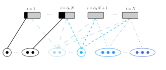
Figure 7: The family of instances generating the upper bound on MSVV when all external traffic arrives first.

First, we verify that the EFET is equal to $\beta$ in the limit as $N$ gets large.

$$\frac{1}{NC}\sum_{i=1}^{\hat{\alpha}_{1}N}C\left(1-\left(\frac{(1-\hat{\alpha}_{1})N}{(1-\hat{\alpha}_{1})N+1}\right)^{i}\right) =\frac{1}{NC}\sum_{i=1}^{\hat{\alpha}_{1}N}\left[C\left(1-\left(1-\frac{1}{(1-\hat{\alpha}_{1})N+1}\right)^{i}\right)\right]$$

$$\xrightarrow{N\rightarrow\infty}\int_{0}^{\hat{\alpha}_{1}}\left[1-\text{exp}\left(\frac{-x}{1-\hat{\alpha}_{1}}\right)\ \partial x\right]$$ (70)

$$=\left(\hat{\alpha}_{1}+(1-\hat{\alpha}_{1})\left(\text{exp}\left(\frac{-\hat{\alpha}_{1}}{1-\hat{\alpha}_{1}}\right)-1\right)\right)$$

$$=\beta$$ (71)

In (70), we use the fact that $(1-1/n)^{nx}$ approaches $\text{exp}^{-x}$ as $n$ approaches infinity. Furthermore, (71) follows by applying the definition of $\hat{\alpha}_{1}$. Next, we analyze the value of MSVV and OPT on the above family of instances via the following two claims.

Claim 3

For any ${EFET}$ $\beta$, the fraction of total capacity filled under MSVV on $\mathcal{I}_{2}(\beta)$ is at most $\hat{\alpha}_{2}$.

Proof.

Proof of Claim 3 To prove this claim, we will bound the amount of filled capacity for each opportunity under MSVV. First, we will show that the $\hat{\alpha}_{1}N$ opportunities that receive external traffic do not receive any matches from internal traffic; i.e., for each $i\in[\hat{\alpha}_{1}N]$, we will show that $\textnormal{{MSVV}}_{i,T}=C\left(1-\left(\frac{(1-\hat{\alpha}_{1})N}{(1-\hat{\alpha}_{1})N+1}\right)^{i}\right)$. Suppose towards a contradiction that there exists some opportunity $j\in[\hat{\alpha}_{1}N]$ which receives a match from internal traffic under MSVV. Due to restrictions on compatibility, this match must have come from one of the first $j$ batches of internal traffic, which in total represents

$$\sum_{i=1}^{j}\Delta_{i}=\sum_{i=1}^{j}C\left(\frac{(1-\hat{\alpha}_{1})N}{(1-\hat{\alpha}_{1})N+1}\right)^{i}=C\left((1-\hat{\alpha}_{1})N\right)\left(1-\left(\frac{(1-\hat{\alpha}_{1})N}{(1-\hat{\alpha}_{1})N+1}\right)^{j}\right)$$ (72)

internal traffic volunteers. We are supposing that one of these volunteers was allocated to opportunity $j$. In that case, due to the pigeonhole principle, there must be at least one opportunity $j^{\prime}$ – from among the $(1-\hat{\alpha}_{1})N$ opportunities that did not receive external traffic – with a filled capacity strictly less than $C\left(1-\left(\frac{(1-\hat{\alpha}_{1})N}{(1-\hat{\alpha}_{1})N+1}\right)^{j}\right)$ upon the arrival of the last volunteer in batch $j$. By definition, MSVV should never have recommended $j$ ahead of $j^{\prime}$, giving us a contradiction.

Next, we show that each opportunity $i\in\{\hat{\alpha}_{1}N+1,\dots,N\}$ has a filled capacity of

$$\textnormal{{MSVV}}_{i,T}=\min\left\{C,C\left(1-\left(\frac{(1-\hat{\alpha}_{1})N}{(1-\hat{\alpha}_{1})N+1}\right)^{\hat{\alpha}_{1}N}+\sum_{j=\hat{\alpha}_{1}N+1}^{i}\frac{1}{N-j+1}\right)\right\}.$$

Note that in this matching setting, MSVV recommends opportunities to equalize their fill rate. Thus, after the arrival of the ${\hat{\alpha}_{1}N}$^th batch of volunteers, all opportunities $j\in\{\hat{\alpha}_{1}N+1,\dots,N\}$ have an equal amount of filled capacity of $C\left(1-\left(\frac{(1-\hat{\alpha}_{1})N}{(1-\hat{\alpha}_{1})N+1}\right)^{\hat{\alpha}_{1}N}\right)$, based on the analysis in the above paragraph (i.e., Equation (72)). For the subsequent batches of volunteers, i.e., for $j\in\{\hat{\alpha}_{1}N+1,\dots,\hat{\alpha}_{2}N\}$, MSVV will maintain an equal fill rate among all compatible opportunities by evenly distributing the $\Delta_{j}=C$ arriving volunteers in batch $j$ among the $N-j+1$ compatible opportunities. After the final arrival in batch $\hat{\alpha}_{2}N$, all remaining compatible opportunities will have reached their capacity. Consequently, after the final arrival in batch $j$ (which is the last volunteer compatible with opportunity $j$), opportunity $j$ will either have reached capacity or will have a filled capacity of

$$C\left(1-\left(\frac{(1-\hat{\alpha}_{1})N}{(1-\hat{\alpha}_{1})N+1}\right)^{\hat{\alpha}_{1}N}\right)+\sum_{j=\hat{\alpha}_{1}N+1}^{i}\frac{C}{N-j+1}.$$

To compute the fraction of total capacity filled under MSVV on $\mathcal{I}_{2}(\beta)$, we then take an average over the fill rate of all opportunities. To that end, we first compute the fill rate for each opportunity in the limit as the number of opportunities approaches infinity.

For $i\in[\hat{\alpha}_{1}N]$,

$$\textsc{FR}_{i,T}\quad=\quad 1-\left(\frac{(1-\hat{\alpha}_{1})N}{(1-\hat{\alpha}_{1})N+1}\right)^{i}$$

Each opportunity $i\in\{\hat{\alpha}_{1}N+1,\dots,\hat{\alpha}_{2}N\}$ will not reach capacity, and thus its fill rate approaches:

$$\textsc{FR}_{i,T}\quad =\quad 1-\left(\frac{(1-\hat{\alpha}_{1})N}{(1-\hat{\alpha}_{1})N+1}\right)^{\hat{\alpha}_{1}N}+\sum_{j=\hat{\alpha}_{1}N+1}^{i}\frac{1}{N-j+1}$$

$$=\quad 1-\left(\frac{(1-\hat{\alpha}_{1})N}{(1-\hat{\alpha}_{1})N+1}\right)^{\hat{\alpha}_{1}N}+\sum_{k=N-i+1}^{(1-\hat{\alpha}_{1})N}\frac{1}{k}$$

It is easy to verify algebraically that for $i=\hat{\alpha}_{2}N$, the fill rate of opportunity $i$, $\textsc{FR}_{i,T}$, asymptotically approaches $1$. The remaining opportunities reach capacity.

With this in mind, the fraction of filled capacity under MSVV can be computed as follows:

$$\frac{1}{N}\sum_{i\in[N]}\textsc{FR}_{i,T}= \frac{1}{N}\left(\sum_{i=1}^{\hat{\alpha}_{1}N}\left(1-\left(\frac{(1-\hat{\alpha}_{1})N}{(1-\hat{\alpha}_{1})N+1}\right)^{i}\right)\right.$$

$$\left.\qquad\quad\quad+\sum_{i=\hat{\alpha}_{1}N+1}^{\hat{\alpha}_{2}N}\left(1-\left(\frac{(1-\hat{\alpha}_{1})N}{(1-\hat{\alpha}_{1})N+1}\right)^{\hat{\alpha}_{1}N}+\sum_{k=N-i+1}^{(1-\hat{\alpha}_{1})N}\frac{1}{k}\right)+\sum_{i=\hat{\alpha}_{2}N+1}^{N}1\right)$$

$$\xrightarrow{N\rightarrow\infty} \int_{0}^{\hat{\alpha}_{1}}1-\text{exp}\left(\frac{-x}{1-\hat{\alpha}_{1}}\right)\ \partial x+\int_{\hat{\alpha}_{1}}^{\hat{\alpha}_{2}}1-\text{exp}\left(\frac{-\hat{\alpha}_{1}}{1-\hat{\alpha}_{1}}\right)+\log\left(\frac{1-\hat{\alpha}_{1}}{1-x}\right)\ \partial x+(1-\hat{\alpha}_{2})$$ (73)

$$= \hat{\alpha}_{1}-(1-\hat{\alpha}_{1})\left(1-\text{exp}\left(\frac{-\hat{\alpha}_{1}}{1-\hat{\alpha}_{1}}\right)\right)+(\hat{\alpha}_{2}-\hat{\alpha}_{1})\left[1-\text{exp}\left(\frac{-\hat{\alpha}_{1}}{1-\hat{\alpha}_{1}}\right)\right]$$

$$\qquad\quad\quad+\int_{\hat{\alpha}_{1}}^{\hat{\alpha}_{2}}\log\left(\frac{1-\hat{\alpha}_{1}}{1-x}\right)\ \partial x+(1-\hat{\alpha}_{2})$$

$$= (1-\hat{\alpha}_{2})\Big{(}\text{{exp}}\big{(}-\hat{\alpha}_{1}/(1-\hat{\alpha}_{1})\big{)}+\log\big{(}(1-\hat{\alpha}_{2})/(1-\hat{\alpha}_{1})\big{)}\Big{)}+\hat{\alpha}_{2}$$

$$= \hat{\alpha}_{2}$$

In (73), we again use the fact that $(1-1/n)^{nx}$ approaches $e^{-x}$ as $n$ approaches infinity. Furthermore, we use the fact that $\sum_{k=yn}^{xn}1/k$ approaches $\log(x/y)$ as $n$ approaches infinity. The last equality comes from applying the definition of $\hat{\alpha}_{2}$ to see that $\log\big{(}(1-\hat{\alpha}_{2})/(1-\hat{\alpha}_{1})\big{)}=-\text{{exp}}\big{(}-\hat{\alpha}_{1}/(1-\hat{\alpha}_{1})\big{)}$. This completes the proof of Claim 3. ∎

Claim 4

For any EFET $\beta$, OPT fills all capacity on $\mathcal{I}_{2}(\beta)$.

Proof.

Proof of Claim 4 Consider a solution which matches all external traffic and then matches each of the $\Delta_{i}$ internal traffic volunteers in batch $i$ to opportunity $i$. To see why such a solution gives a perfect matching, note that each opportunity $i\in\{1,\dots,\hat{\alpha}_{1}N\}$ will receive $C\left(1-\left(\frac{(1-\hat{\alpha}_{1})N}{(1-\hat{\alpha}_{1})N+1}\right)^{i}\right)$ matches from external traffic and $\Delta_{i}=C\left(\frac{(1-\hat{\alpha}_{1})N}{(1-\hat{\alpha}_{1})N+1}\right)^{i}$ matches from internal traffic, leading to a total of $C$ matches. Each opportunity $i\in\{\hat{\alpha}_{1}N+1,\dots,N\}$ will receive $\Delta_{i}=C$ matches (all from internal traffic). Thus, each opportunity is filled to capacity under this solution, which implies that the optimal solution must also fill all capacity. ∎

Combining Claims 3 and 4, we see that MSVV only fills a fraction $\hat{\alpha}_{2}$ of the capacity filled by OPT on this family of instances, which provides a parameterized upper bound on the competitive ratio of MSVV in this setting.

8.6 Proof of Proposition 3 (Section 4.1)

We prove Proposition 3 in two steps. In Step (a), fixing an instance $\mathcal{I}\in\mathcal{I}_{\beta}$, we show that the expected fraction of capacity filled by external traffic is $\beta$ under both AC and OPT. Then, in Step (b) we establish a lower bound on the amount of capacity filled by internal traffic under AC, which depends on the amount of capacity filled by internal traffic under OPT. Together, these steps enable us to place a lower bound on the competitive ratio of AC, where the bound is parameterized by the EFET $\beta$.

Step (a): Both OPT and AC always recommend the targeted opportunity $i^{*}_{t}$ to external traffic. Since external traffic is assumed to arrive before all internal traffic, this external traffic will fill a fraction of capacity given by

$$\beta(\mathcal{I})=\frac{\sum_{i\in[n]}\mathbb{E}\left[\min\{c_{i},\sum_{t\in\mathcal{V}^{\textsc{ext}}}\mathbbm{1}[\xi_{t}(S^{i^{*}_{t}}_{t})=i]\}\right]}{\sum_{i\in[n]}c_{i}}.$$

We note that this fraction of capacity is exactly equivalent to the definition of the EFET (see Definition 2), which is equal to $\beta$ for any instance $\mathcal{I}\in\mathcal{I}_{\beta}$.

Step (b): Fixing an instance $\mathcal{I}$, we now turn our attention to lower-bounding the expected amount of capacity filled by internal traffic under the AC algorithm, where the expectation is taken over sample paths $\bm{\omega}=\{\bm{\omega}_{1},\dots,\bm{\omega}_{T}\}$, i.e., realizations of random variables that govern volunteer choices in this instance. Formally, we interpret $\bm{\omega}_{t}$ as a vector of length $n+1$, where the $i$^th component of $\bm{\omega}_{t}$ (denoted $\omega_{i,t}$) indicates volunteer $t$’s sign-up decision if the platform were to recommend opportunity $i$. For a fixed instance $\mathcal{I}$ and a fixed sample path $\bm{\omega}$, we use $\widehat{\textnormal{{AC}}}$ to denote the amount of capacity filled by internal traffic under the AC algorithm.

Our lower bound on $\mathbb{E}_{\bm{\omega}}\big{[}\widehat{\textnormal{{AC}}}\big{]}$ will depend on the expected amount of capacity filled by internal traffic under OPT, which we likewise denote with $\mathbb{E}_{\bm{\omega}}\big{[}\widehat{\textnormal{{OPT}}}\big{]}$ (We note that the expectations are taken with respect to all possible realizations of volunteer sign-up decisions, i.e., all sample paths $\bm{\omega}$.) Note that in this step of the proof, we are concerned only with the remaining capacities for each opportunity $i$ after the arrival of external traffic (denoted $\hat{c}_{i}$), which depends on the realizations of sign-ups made by external traffic. As such, $\hat{c}_{i}$ depends not only on the instance $\mathcal{I}$, but also on the sample path $\bm{\omega}$.

To provide such a lower bound, we leverage the LP-free approach developed in Goyal and Udwani [2019] and Goyal et al. [2020], which involves the creation of path-based pseudo-rewards. (For a more complete discussion of the intuition behind this approach, we kindly refer to the proof sketch of Theorem 3 in Section 5.) For a fixed instance $\mathcal{I}$ and a fixed sample path $\bm{\omega}$, we define the pseudo-rewards $\hat{L}_{t}$ for all $t\in\mathcal{V}^{\textsc{int}}$ and $\hat{K}_{i}$ for all $i\in[n]$ according to the following:

$$\hat{L}_{t} =\sum_{i\in[n]}\psi(\textsc{FR}_{i,t-1})\mathbbm{1}[\xi_{t}(S^{\textnormal{{OPT}}}_{t})=i]$$ (74)

$$\hat{K}_{i} =\sum_{t\in\mathcal{V}^{\textsc{int}}}\left(1-\psi(\textsc{FR}_{i,t-1})\right)\mathbbm{1}[\xi_{t}(S^{\textnormal{{AC}}}_{t})=i],$$ (75)

where we remind that under the AC algorithm, $\textsc{FR}_{i,t-1}=\textnormal{{AC}}_{i,t}^{\textsc{int}}/(c_{i}-\textnormal{{AC}}_{i,t}^{\textsc{ext}})$. This is equivalent to $\textnormal{{AC}}_{i,t}^{\textsc{int}}/\hat{c}_{i}$ in our warm-up setting where external traffic arrives first and the remaining capacity for opportunity $i$ is given by $\hat{c}_{i}$. We now prove that the expected sum of these pseudo-rewards serves as a lower bound on the expected value of $\widehat{\textnormal{{AC}}}$.

Lemma 11

For any instance $\mathcal{I}$,

$$\mathbbm{E}_{\bm{\omega}}\big{[}\widehat{\textnormal{{AC}}}\big{]}\quad\geq\quad\mathbbm{E}_{\bm{\omega}}\left[\sum_{t\in\mathcal{V}^{\textsc{int}}}\hat{L}_{t}+\sum_{i\in[n]}\hat{K}_{i}\right],$$ (76)

where $\hat{L}_{t}$ and $\hat{K}_{i}$ are defined in (74) and (75), respectively.

Proof.

Proof of Lemma 11: The proof follows from the definition of $\hat{L}_{t}$ and $\hat{K}_{i}$ as well as the design of the AC algorithm:

$$\mathbbm{E}_{\bm{\omega}}\big{[}\widehat{\textnormal{{AC}}}\big{]} =\mathbb{E}_{\bm{\omega}}\left[\sum_{t\in\mathcal{V}^{\textsc{int}}}\sum_{i\in[n]}\mathbbm{1}[\xi_{t}(S^{\textnormal{{AC}}}_{t})=i]\right]$$ (77)

$$=\mathbb{E}_{\bm{\omega}}\left[\sum_{t\in\mathcal{V}^{\textsc{int}}}\sum_{i\in[n]}\psi(\textsc{FR}_{i,t-1})\mathbbm{1}[\xi_{t}(S^{\textnormal{{AC}}}_{t})=i]+\sum_{t\in\mathcal{V}^{\textsc{int}}}\sum_{i\in[n]}\Big{(}1-\psi(\textsc{FR}_{i,t-1})\Big{)}\mathbbm{1}[\xi_{t}(S^{\textnormal{{AC}}}_{t})=i]\right]$$ (78)

$$\geq\mathbb{E}_{\bm{\omega}}\left[\sum_{t\in\mathcal{V}^{\textsc{int}}}\sum_{i\in[n]}\psi(\textsc{FR}_{i,t-1})\mathbbm{1}[\xi_{t}(S^{\textnormal{{OPT}}}_{t})=i]+\sum_{i\in[n]}\hat{K}_{i}\right]$$ (79)

$$=\mathbbm{E}_{\bm{\omega}}\left[\sum_{t\in\mathcal{V}^{\textsc{int}}}\hat{L}_{t}+\sum_{i\in[n]}\hat{K}_{i}\right]$$ (80)

Equality (77) holds because the AC algorithm will never recommend an opportunity that has already reached capacity to internal traffic. Consequently, the amount of capacity filled by internal traffic under the AC algorithm is exactly equal to the numbers of sign-ups from internal traffic.

Inequality (79) follows from the AC algorithm’s optimality condition (see Algorithm 2), which ensures that it recommends the opportunity that maximizes the weighted probability of generating a sign-up (where the weight for opportunity $i$ at time $t$ is given by $\psi(\textsc{FR}_{i,t-1})$). As OPT does not have foreknowledge of the realization of the sign-up decisions of internal traffic, the recommendation provided by OPT to any volunteer must be independent of their sign-up realization. Hence, the inequality holds. Applying the definition of the pseudo-rewards $\hat{L}_{t}$ for $t\in\mathcal{V}^{\textsc{int}}\setminus\mathcal{V}^{0}$ completes the proof of Lemma 11.

∎

Next, we place a lower bound on the expected sum of the pseudo-rewards, which depends on the amount of capacity of each opportunity $i$ filled by internal traffic under OPT along a fixed sample path, which we denote by $\widehat{\textnormal{{OPT}}}_{i}$.

Lemma 12

For any instance $\mathcal{I}$,

$$\mathbbm{E}_{\bm{\omega}}\left[\sum_{t\in\mathcal{V}^{\textsc{int}}}\hat{L}_{t}+\sum_{i\in[n]}\hat{K}_{i}\right]\quad\geq\quad(1-1/e)\mathbbm{E}_{\bm{\omega}}\left[\widehat{\textnormal{{OPT}}}\right]-\sum_{i\in[n]}\mathbbm{E}_{\bm{\omega}}\left[\mathbbm{1}\big{[}\widehat{\textnormal{{OPT}}}_{i}=\hat{c}_{i}\big{]}\right]$$ (81)

Proof.

Proof of Lemma 12: We will prove this claim along each sample path $\bm{\omega}$ by separately placing lower bounds on the $\hat{L}_{t}$ pseudo-rewards and the $\hat{K}_{i}$ pseudo-rewards. For the former,

$$\sum_{t\in\mathcal{V}^{\textsc{int}}}\hat{L}_{t}\quad =\quad\sum_{t\in\mathcal{V}^{\textsc{int}}}\sum_{i\in[n]}\psi(\textsc{FR}_{i,t-1})\mathbbm{1}[\xi_{t}(S^{\textnormal{{OPT}}}_{t})=i]$$ (82)

$$\geq\quad\sum_{t\in\mathcal{V}^{\textsc{int}}}\sum_{i\in[n]}\psi(\textsc{FR}_{i,T})\mathbbm{1}[\xi_{t}(S^{\textnormal{{OPT}}}_{t})=i]$$ (83)

$$=\quad\sum_{i\in[n]}\widehat{\textnormal{{OPT}}}_{i}\psi\left(\textsc{FR}_{i,T}\right)$$ (84)

Equality in (82) follows from the definition of $\hat{L}_{t}$. Inequality in (83) holds because $\psi$ is a decreasing function in its argument, and $\textsc{FR}_{i,T}\geq\textsc{FR}_{i,t-1}$ for all $t\in[T]$. All other steps are algebraic.

We now turn our attention to the $\hat{K}_{i}$ pseudo-rewards:

$$\hat{K}_{i}\quad= \quad\sum_{t\in\mathcal{V}^{\textsc{int}}}\left(1-\psi(\textsc{FR}_{i,t-1})\right)\mathbbm{1}[\xi_{t}(S^{\textnormal{{AC}}}_{t})=i]$$ (85)

$$= \quad\sum_{t\in\mathcal{V}^{\textsc{int}}}\left(1-\psi\left(\frac{\textnormal{{AC}}_{i,t-1}^{\textsc{int}}}{\hat{c}_{i}}\right)\right)\mathbbm{1}[\xi_{t}(S^{\textnormal{{AC}}}_{t})=i]$$ (86)

$$\quad= \quad\sum_{\in[\textnormal{{AC}}_{i,T}^{\textsc{int}}]}\left(1-\psi\left(\frac{}{\hat{c}_{i}}\right)\right)$$ (87)

$$\quad= \quad e^{\frac{-1}{\hat{c}_{i}}}\sum_{\in[\textnormal{{AC}}_{i,T}^{\textsc{int}}]}\left(1-\psi\left(\frac{}{\hat{c}_{i}}\right)\right)$$ (88)

$$\quad\geq \quad e^{\frac{-1}{\hat{c}_{i}}}\int_{0}^{\textnormal{{AC}}_{i,T}^{\textsc{int}}}1-\psi(x/\hat{c}_{i})\ \partial x$$ (89)

$$\quad= \quad e^{\frac{-1}{\hat{c}_{i}}}\hat{c}_{i}\left(1-\psi\left(\textsc{FR}_{i,T}\right)-1/e\right)$$ (90)

$$\quad\geq \quad(\hat{c}_{i}-1)\left(1-\psi\left(\textsc{FR}_{i,T}\right)-1/e\right)$$ (91)

Equality in (87) holds because the counter $\textnormal{{AC}}_{i,t}^{\textsc{int}}$ will increase by $1$ for any $t\in\mathcal{V}^{\textsc{int}}$ where $\xi_{t}(S^{\textnormal{{AC}}}_{t})=i$. The summation in (87) represents a left Riemann sum of an increasing function. In (88), we utilize the fact that for any , $1-\psi(()/\hat{c}_{i})=e^{-1/\hat{c}_{i}}(1-\psi(/\hat{c}_{i}))$. As the summation in (88) is now a right Riemann sum of an increasing function, we bound the sum with an appropriate integral in (89). Finally, (91) holds because $e^{-x}\geq 1-x$ for any $x$.

Combining (84) and (91), we see that for each sample path $\bm{\omega}$,

$$\sum_{t\in\mathcal{V}^{\textsc{int}}}\hat{L}_{t}+\sum_{i\in[n]}\hat{K}_{i} \geq\sum_{i\in[n]}\widehat{\textnormal{{OPT}}}_{i}\psi\left(\textsc{FR}_{i,T}\right)+(\hat{c}_{i}-1)\left(1-\psi\left(\textsc{FR}_{i,T}\right)-1/e\right)$$ (92)

$$\geq\sum_{i\in[n]}\left(\widehat{\textnormal{{OPT}}}_{i}-\mathbbm{1}[\widehat{\textnormal{{OPT}}}_{i}=\hat{c}_{i}]\right)\psi\left(\textsc{FR}_{i,T}\right)+\left(\widehat{\textnormal{{OPT}}}_{i}-\mathbbm{1}[\widehat{\textnormal{{OPT}}}_{i}=\hat{c}_{i}]\right)\left(1-\psi\left(\textsc{FR}_{i,T}\right)-1/e\right)$$ (93)

$$=(1-1/e)\sum_{i\in[n]}\left(\widehat{\textnormal{{OPT}}}_{i}-\mathbbm{1}\big{[}\widehat{\textnormal{{OPT}}}_{i}=\hat{c}_{i}\big{]}\right)$$ (94)

$$\geq(1-1/e)\cdot\widehat{\textnormal{{OPT}}}-\sum_{i\in[n]}\mathbbm{1}\big{[}\widehat{\textnormal{{OPT}}}_{i}=\hat{c}_{i}\big{]}$$ (95)

Inequality in (93) comes from noting that $\left(\widehat{\textnormal{{OPT}}}_{i}-\mathbbm{1}\big{[}\widehat{\textnormal{{OPT}}}_{i}=\hat{c}_{i}\big{]}\right)$ cannot exceed either $\widehat{\textnormal{{OPT}}}_{i}$ or $\hat{c}_{i}-1$. (We note that the binary indicator $\mathbbm{1}\big{[}\widehat{\textnormal{{OPT}}}_{i}=\hat{c}_{i}\big{]}$ is equal to $1$ if and only if opportunity $i$ reaches capacity under OPT along the fixed sample path $\bm{\omega}$.) Taking expectation across all sample paths completes the proof of Lemma 12. ∎

Combining Lemmas 11 and 12, we see that we can bound the expected amount of capacity filled by internal traffic under AC via the following inequality:

$$\mathbbm{E}_{\bm{\omega}}\big{[}\widehat{\textnormal{{AC}}}\big{]}\quad\geq\quad(1-1/e)\mathbbm{E}_{\bm{\omega}}\big{[}\widehat{\textnormal{{OPT}}}\big{]}-\sum_{i\in[n]}\mathbbm{E}_{\bm{\omega}}\left[\mathbbm{1}\big{[}\widehat{\textnormal{{OPT}}}_{i}=\hat{c}_{i}\big{]}\right]$$ (96)

Together with Step (a), we have shown that for any instance $\mathcal{I}\in\mathcal{I}_{\beta}$,

$$\frac{\mathbbm{E}_{\bm{\omega}}\left[\textnormal{{AC}}\right]}{\mathbbm{E}_{\bm{\omega}}\left[\textnormal{{OPT}}\right]}\quad =\quad\frac{\beta\cdot\sum_{i\in[n]}c_{i}+\mathbbm{E}_{\bm{\omega}}\left[\widehat{\textnormal{{AC}}}\right]}{\beta\cdot\sum_{i\in[n]}c_{i}+\mathbbm{E}_{\bm{\omega}}\left[\widehat{\textnormal{{OPT}}}\right]}$$ (97)

$$\geq\quad\frac{\beta\cdot\sum_{i\in[n]}c_{i}+(1-1/e)\mathbbm{E}_{\bm{\omega}}\left[\widehat{\textnormal{{OPT}}}\right]-\sum_{i\in[n]}\mathbbm{E}_{\bm{\omega}}\left[\mathbbm{1}\big{[}\widehat{\textnormal{{OPT}}}_{i}=\hat{c}_{i}\big{]}\right]}{\beta\cdot\sum_{i\in[n]}c_{i}+\mathbbm{E}_{\bm{\omega}}\left[\widehat{\textnormal{{OPT}}}\right]}$$ (98)

$$=\quad\frac{\beta\cdot\sum_{i\in[n]}c_{i}+(1-1/e)\mathbbm{E}_{\bm{\omega}}\left[\widehat{\textnormal{{OPT}}}\right]}{\beta\cdot\sum_{i\in[n]}c_{i}+\mathbbm{E}_{\bm{\omega}}\left[\widehat{\textnormal{{OPT}}}\right]}-\frac{\sum_{i\in[n]}\mathbbm{E}_{\bm{\omega}}\left[\mathbbm{1}\big{[}\widehat{\textnormal{{OPT}}}_{i}=\hat{c}_{i}\big{]}\right]}{\mathbbm{E}_{\bm{\omega}}\left[\textnormal{{OPT}}\right]}$$ (99)

$$\geq\quad\frac{\beta\cdot\sum_{i\in[n]}c_{i}+(1-1/e)\mathbbm{E}_{\bm{\omega}}\left[\widehat{\textnormal{{OPT}}}\right]}{\beta\cdot\sum_{i\in[n]}c_{i}+\mathbbm{E}_{\bm{\omega}}\left[\widehat{\textnormal{{OPT}}}\right]}-\underline{c}^{-1}$$ (100)

$$\geq\quad\beta+(1-\beta)(1-1/e)-\underline{c}^{-1}$$ (101)

Equality in (97) comes from applying the result of Step (a), while inequality in (98) comes from applying the result of Step (b). Equality in (98) follows from the definition of OPT. To see that (100) holds, we first fix a sample path. Along that sample path, if $\widehat{\textnormal{{OPT}}}_{i}=\hat{c}_{i}$, then opportunity $i$ must have reached capacity under OPT. The capacity of opportunity $i$ is at least $\underline{c}$. Thus, along every sample path, $\textnormal{{OPT}}\geq\underline{c}\sum_{i\in[n]}\mathbbm{E}_{\bm{\omega}}\left[\mathbbm{1}\big{[}\widehat{\textnormal{{OPT}}}_{i}=\hat{c}_{i}\big{]}\right]$. This is a sufficient condition to establish (100).

Finally, (101) comes from noting that the expression in (100) is decreasing in $\mathbbm{E}_{\bm{\omega}}\left[\widehat{\textnormal{{OPT}}}\right]$, which can be at most $\mathbbm{E}_{\bm{\omega}}\left[\sum_{i\in[n]}\hat{c}_{i}\right]$. Furthermore, $\mathbbm{E}_{\bm{\omega}}\left[\sum_{i\in[n]}\hat{c}_{i}\right]=(1-\beta)\sum_{i\in[n]}c_{i}$. We then plug in this upper bound for $\mathbbm{E}_{\bm{\omega}}\left[\widehat{\textnormal{{OPT}}}\right]$. This final inequality establishes a lower bound for any instance $\mathcal{I}\in\mathcal{I}_{\beta}$. Thus, it represents a lower bound on the competitive ratio parameterized by the EFET $\beta$, as desired. This completes the proof of Proposition 3.

8.7 Upper Bound on MSVV in General Settings (Section 4.3)

In the following proposition, we provide an upper bound on the competitive ratio of MSVV as a function of the EFET $\beta$.

Proposition 4 (Upper Bound on MSVV)

For any effective fraction of external traffic $\beta$ and any minimum capacity, MSVV cannot achieve a competitive ratio better than

$$\begin{cases}1-1/e,&\beta\leq 1/e\\ \min\left\{\alpha_{2},\alpha_{3}\right\},&\beta>1/e\end{cases}$$

where, for $\beta>1/e$, $\alpha_{2}$ is given by

$$\alpha_{2}=1-\frac{1-\alpha_{1}}{\text{\emph{exp}}\left(\text{\emph{exp}}(-\alpha_{1}/(1-\alpha_{1}))\right)}$$

and $\alpha_{1}$ and is the unique solution in $[0,1]$ to $\beta=\alpha_{1}+(1-\alpha_{1})\Big{(}\text{\emph{exp}}\big{(}-\alpha_{1}/(1-\alpha_{1})\big{)}-1\Big{)}+\frac{1-\alpha_{1}}{\text{\emph{exp}}\left(\text{\emph{exp}}(-\alpha_{1}/(1-\alpha_{1}))\right)}$. In addition,

$$\alpha_{3}=\min_{\alpha_{4}\in[0,\beta]}1-\frac{1-\beta}{1-\alpha_{4}}\left(\alpha_{5}+(1-\alpha_{6})\log\left(\frac{1-\alpha_{5}}{1-\alpha_{6}}\right)\right),$$

where $\alpha_{5}=\min\{1-\alpha_{4},\frac{\alpha_{4}(\beta-\alpha_{4})}{1-\beta}\}$ and $\alpha_{6}=\min\{1-\alpha_{4},1-(1-\alpha_{5})/e\}$.

Proof.

Proof of Proposition 4 The first part of Proposition 4 – which establishes an upper bound of $1-1/e$ when $\beta\leq 1/e$ – follows immediately from Theorem 1, in which we prove such an upper bound on the competitive ratio of any online algorithm.

We prove the remainder of this proposition in two claims by showing two different upper bounds ($\alpha_{2}$ and $\alpha_{3}$) on the competitive ratio of MSVV parameterized by the effective fraction of external traffic $\beta$. Proposition 4 follows by taking the minimum of the two upper bounds for a given $\beta$.

To prove each claim, we construct a family of instances parameterized by $\beta$. We then evaluate the value of MSVV on that family of instances relative to the value of OPT. Both of the instances that we design leverage the fact that the notion of a fill rate under MSVV does not distinguish between internal and external traffic. As a result, MSVV may mistakenly withhold internal traffic from opportunities that have previously received external traffic. Furthermore, all instances leverage the triangular structure of our general hardness result (see Appendix 8.1).

Claim 5

For any effective fraction of external traffic $\beta\in(1/e,1]$, the competitive ratio of MSVV is at most

$$1-\frac{1-\alpha_{1}}{\text{\emph{exp}}\left(\text{\emph{exp}}(-\alpha_{1}/(1-\alpha_{1}))\right)}$$ (102)

where $\alpha_{1}$ is the unique solution in $[0,1]$ to $\beta=\alpha_{1}+(1-\alpha_{1})\Big{(}\text{\emph{exp}}\big{(}-\alpha_{1}/(1-\alpha_{1})\big{)}-1\Big{)}+\frac{1-\alpha_{1}}{\text{\emph{exp}}\left(\text{\emph{exp}}(-\alpha_{1}/(1-\alpha_{1}))\right)}$.

Proof.

Proof of Claim 5 To prove this claim, we construct a family of instances $\mathcal{I}_{3}(\beta)$ parameterized by the EFET $\beta$. (As we will highlight below, this family of instances will have a close relationship to the family of instances $\mathcal{I}_{2}(\beta)$, introduced in the proof of Proposition 2.) In each instance, there are a large number of opportunities $N$, each with identical large capacity $C$. The arrival sequence consists of $NC$ volunteers, and for a given effective fraction of external traffic $\beta$, the first $\beta NC$ of these volunteers are external traffic. All volunteers have conversion probabilities of $1$ or $0$, and if $\mu_{i,t}=1$ (resp. 0), we will refer to opportunity $i$ and volunteer $t$ as compatible (resp. incompatible).

To help describe the compatibility structure of the arriving volunteers, we first define constants ${\alpha}_{1}$ and ${\alpha}_{2}$. For $\beta\leq 1/e$, we define $\alpha_{1}=0$, while for $\beta>1/e$, we define $\alpha_{1}$ as the unique solution in $[0,1]$ to

$$\beta={\alpha}_{1}+(1-{\alpha}_{1})\Big{(}\text{{exp}}\big{(}-{\alpha}_{1}/(1-{\alpha}_{1})\big{)}-1\Big{)}+\frac{1-\alpha_{1}}{\text{{exp}}\left(\text{{exp}}(-\alpha_{1}/(1-\alpha_{1}))\right)},$$

and $\alpha_{2}$ is defined as

$${\alpha}_{2}=1-\frac{1-{\alpha}_{1}}{\text{{exp}}\left(\text{{exp}}(-{\alpha}_{1}/(1-{\alpha}_{1}))\right)}.$$

The arrival sequence begins with external traffic volunteers for the first $\alpha_{1}N$ opportunities. Specifically, for each opportunity $i\in\{1,\dots,{\alpha}_{1}N\}$, there are $C\left(1-\left(\frac{(1-{\alpha}_{1})N}{(1-{\alpha}_{1})N+1}\right)^{i}\right)$ compatible external traffic arrivals for that opportunity. After the arrival of these volunteers, the internal traffic arrives, according to the following compatibility structure: for each opportunity $i\in\{1,\dots,{\alpha}_{2}N\}$, there is a batch of $\Delta_{i}$ sequentially-arriving homogeneous volunteers. The batches consist of $\Delta_{i}=C\left(\frac{(1-{\alpha}_{1})N}{(1-{\alpha}_{1})N+1}\right)^{i}$ volunteers for each $i\in\{1,\dots,{\alpha}_{1}N\}$, and they consist of $\Delta_{i}=C$ volunteers  for each $i\in\{\alpha_{1}N+1,\dots,{\alpha}_{2}N\}$. Volunteers in batch $i$ are compatible with all opportunities $j\geq i$. Finally, the arrival sequence concludes with $(1-\alpha_{2})N$ batches of $C$ external traffic volunteers, where each batch views (and is compatible with) one opportunity $i\in\{{\alpha}_{2}N+1,\dots,N\}$.

Before analyzing this family of instances, we make two observations. First, this arrival sequence is quite similar to the arrival sequence in the family of instances $\mathcal{I}_{2}(\beta)$, which are visualized in Figure 7 and which provide our upper bound on MSVV in the setting where all external traffic arrives first (see Proposition 2). The only difference comes from the last batches of arrivals, which are external traffic in this family of instances (as opposed to internal traffic with broader compatibility, as in $\mathcal{I}_{2}(\beta)$). In both cases, these volunteers are unable to be allocated under MSVV as their compatible opportunities have already reached capacity, whereas these volunteers are allocated under OPT. Hence, the value of MSVV and the value of OPT are both unchanged. Crucially, though, the EFET is different in these two instances, due to the change in source of the last-arriving volunteers. As a result, for a fixed $\beta$, the instance $\mathcal{I}_{2}(\beta)$ and $\mathcal{I}_{3}(\beta)$ differ significantly. Instead, $\mathcal{I}_{2}(\beta)$ and $\mathcal{I}_{3}(\beta+\hat{\alpha}_{2})$ are nearly identical (where $\hat{\alpha}_{2}$ is a function of $\beta$, as defined in the proof of Proposition 2). This relationship means the upper bound provided by the family of instances $\mathcal{I}_{3}(\beta)$ is a non-linear transformation of the upper bound provided by the family of instances $\mathcal{I}_{2}(\beta)$. Furthermore, we remark that in the limit as $\beta$ approaches $1/e$, $\mathcal{I}_{3}(\beta)$ approaches the instance $\mathcal{I}_{1}(1/e)$, which provides our general hardness result presented in Theorem 1.

We now verify that the EFET is equal to $\beta$ in the limit as $N$ gets large.

$$\frac{1}{NC}\left(\sum_{i=1}^{{\alpha}_{1}N}C\left(1-\left(\frac{(1-{\alpha}_{1})N}{(1-{\alpha}_{1})N+1}\right)^{i}\right)+(1-\alpha_{2})NC\right)= \frac{1}{N}\left[\sum_{i=1}^{{\alpha}_{1}N}\left(1-\left(1-\frac{1}{(1-{\alpha}_{1})N+1}\right)^{i}\right)+(1-\alpha_{2})N\right]$$

$$\xrightarrow{N\rightarrow\infty} \int_{0}^{{\alpha}_{1}}\left[1-\text{exp}\left(\frac{-x}{1-{\alpha}_{1}}\right)\ \partial x\right]+(1-\alpha_{2})$$ (103)

$$= \left({\alpha}_{1}+(1-{\alpha}_{1})\left(\text{exp}\left(\frac{-{\alpha}_{1}}{1-{\alpha}_{1}}\right)-1\right)\right)+(1-\alpha_{2})$$

$$= \beta$$ (104)

In (103), we use the fact that $(1-1/n)^{nx}$ approaches $e^{-x}$ as $n$ approaches infinity. Furthermore, (104) follows by applying the definitions of ${\alpha}_{2}$ and ${\alpha}_{1}$. Next, we analyze the value of MSVV and OPT on the above family of instances.

Value of MSVV on Instance $\mathcal{I}_{3}(\beta)$: We will show that for any ${EFET}$ $\beta$, the fraction of total capacity filled under MSVV on $\mathcal{I}_{3}(\beta)$ is at most ${\alpha}_{2}$. To that end, we will first bound the amount of filled capacity for each opportunity under MSVV. First, we will show that the ${\alpha}_{1}N$ opportunities that initially receive external traffic do not receive any matches from internal traffic; i.e., for each $i\in[{\alpha}_{1}N]$, we will show that $\textnormal{{MSVV}}_{i,T}=C\left(1-\left(\frac{(1-{\alpha}_{1})N}{(1-{\alpha}_{1})N+1}\right)^{i}\right)$. Suppose towards a contradiction that there exists some opportunity $j\in[{\alpha}_{1}N]$ which receives a match from internal traffic under MSVV. Due to restrictions on compatibility, this match must have come from one of the first $j$ batches of internal traffic, which in total represents

$$\sum_{i=1}^{j}\Delta_{i}=\sum_{i=1}^{j}C\left(\frac{(1-{\alpha}_{1})N}{(1-{\alpha}_{1})N+1}\right)^{i}=C\left((1-{\alpha}_{1})N\right)\left(1-\left(\frac{(1-{\alpha}_{1})N}{(1-{\alpha}_{1})N+1}\right)^{j}\right)$$

internal traffic volunteers. We are supposing that one of these volunteers was allocated to opportunity $j$. In that case, due to the pigeonhole principle, there must be at least one opportunity $j^{\prime}$ – from among the $(1-{\alpha}_{1})N$ opportunities that did not initially receive external traffic – with a filled capacity strictly less than $C\left(1-\left(\frac{(1-{\alpha}_{1})N}{(1-{\alpha}_{1})N+1}\right)^{j}\right)$ upon the arrival of the last volunteer in batch $j$. By definition, MSVV should never have recommended $j$ ahead of $j^{\prime}$, giving us a contradiction.

Next, we show that each opportunity $i\in\{{\alpha}_{1}N+1,\dots,{\alpha}_{2}N\}$ has a filled capacity of

$$\textnormal{{MSVV}}_{i,T}\leq C\left(1-\left(\frac{(1-{\alpha}_{1})N}{(1-{\alpha}_{1})N+1}\right)^{{\alpha}_{1}N}+\sum_{j={\alpha}_{1}N+1}^{i}\frac{1}{N-j+1}\right).$$ (105)

Note that in this matching setting, MSVV recommends opportunities to equalize their fill rate. Thus, after the arrival of the ${{\alpha}_{1}N}$^th batch of volunteers, all opportunities $j\in\{{\alpha}_{1}N+1,\dots,\alpha_{2}N\}$ have an equal amount of filled capacity of $C\left(1-\left(\frac{(1-{\alpha}_{1})N}{(1-{\alpha}_{1})N+1}\right)^{{\alpha}_{1}N}\right)$, based on the analysis in the above paragraph (i.e., (105)). For the subsequent batches of internal traffic volunteers, i.e., for $j\in\{{\alpha}_{1}N+1,\dots,{\alpha}_{2}N\}$, MSVV will maintain an equal fill rate among all compatible opportunities by evenly distributing the $\Delta_{j}=C$ arriving volunteers in batch $j$ among the $N-j+1$ compatible opportunities. Thus, after the final arrival in batch $j$ (which is the last volunteer compatible with opportunity $j$), opportunity $j$ will have a filled capacity of at most

$$C\left(1-\left(\frac{(1-{\alpha}_{1})N}{(1-{\alpha}_{1})N+1}\right)^{{\alpha}_{1}N}\right)+\sum_{j={\alpha}_{1}N+1}^{i}\frac{C}{N-j+1}.$$

The remaining opportunities (i.e., opportunities $i$ for $i>\alpha_{2}N$) will all have reached capacity following the last arrival in batch $\alpha_{2}N$.

To compute the fraction of total capacity filled under MSVV on $\mathcal{I}_{3}(\beta)$, we then take an average over the fill rate of all opportunities. To that end, we first compute the fill rate for each opportunity in the limit as the number of opportunities approaches infinity.

For $i\in[{\alpha}_{1}N]$,

$$\textsc{FR}_{i,T}\quad=\quad 1-\left(\frac{(1-{\alpha}_{1})N}{(1-{\alpha}_{1})N+1}\right)^{i}$$

Each opportunity $i\in\{{\alpha}_{1}N+1,\dots,{\alpha}_{2}N\}$ has a fill rate which is bounded by:

$$\textsc{FR}_{i,T}\quad =\quad 1-\left(\frac{(1-{\alpha}_{1})N}{(1-{\alpha}_{1})N+1}\right)^{{\alpha}_{1}N}+\sum_{j={\alpha}_{1}N+1}^{i}\frac{1}{N-j+1}$$

$$=\quad 1-\left(\frac{(1-{\alpha}_{1})N}{(1-{\alpha}_{1})N+1}\right)^{{\alpha}_{1}N}+\sum_{k=N-i+1}^{(1-{\alpha}_{1})N}\frac{1}{k}$$

It is easy to verify algebraically that for $i={\alpha}_{2}N$, the fill rate of opportunity $i$, $\textsc{FR}_{i,T}$, asymptotically approaches $1$. The remaining opportunities reach capacity.

With this in mind, the fraction of filled capacity under MSVV can be computed as follows:

$$\frac{1}{N}\sum_{i\in[N]}\textsc{FR}_{i,T}= \ \frac{1}{N}\left(\sum_{i=1}^{{\alpha}_{1}N}\left(1-\left(\frac{(1-{\alpha}_{1})N}{(1-{\alpha}_{1})N+1}\right)^{i}\right)\right.$$

$$\left.\qquad\quad\quad+\sum_{i={\alpha}_{1}N+1}^{{\alpha}_{2}N}\left(1-\left(\frac{(1-{\alpha}_{1})N}{(1-{\alpha}_{1})N+1}\right)^{{\alpha}_{1}N}+\sum_{k=N-i+1}^{(1-{\alpha}_{1})N}\frac{1}{k}\right)+\sum_{i={\alpha}_{2}N+1}^{N}1\right)$$

$$\xrightarrow{N\rightarrow\infty} \int_{0}^{{\alpha}_{1}}1-\text{exp}\left(\frac{-x}{1-{\alpha}_{1}}\right)\ \partial x+\int_{{\alpha}_{1}}^{{\alpha}_{2}}1-\text{exp}\left(\frac{-{\alpha}_{1}}{1-{\alpha}_{1}}\right)+\log\left(\frac{1-{\alpha}_{1}}{1-x}\right)\ \partial x+(1-{\alpha}_{2})$$ (106)

$$= \ {\alpha}_{1}-(1-{\alpha}_{1})\left(1-\text{exp}\left(\frac{-{\alpha}_{1}}{1-{\alpha}_{1}}\right)\right)+({\alpha}_{2}-{\alpha}_{1})\left[1-\text{exp}\left(\frac{-{\alpha}_{1}}{1-{\alpha}_{1}}\right)\right]$$

$$\qquad\quad\quad+\int_{{\alpha}_{1}}^{{\alpha}_{2}}\log\left(\frac{1-{\alpha}_{1}}{1-x}\right)\ \partial x+(1-{\alpha}_{2})$$

$$= \ (1-{\alpha}_{2})\Big{(}\text{{exp}}\big{(}-{\alpha}_{1}/(1-{\alpha}_{1})\big{)}+\log\big{(}(1-{\alpha}_{2})/(1-{\alpha}_{1})\big{)}\Big{)}+{\alpha}_{2}$$

$$= \ {\alpha}_{2}$$

In (106), we again use the fact that $(1-1/n)^{nx}$ approaches $e^{-x}$ as $n$ approaches infinity. Furthermore, we use the fact that $\sum_{k=yn}^{xn}1/k$ approaches $\log(x/y)$ as $n$ approaches infinity. The last equality comes from applying the definition of ${\alpha}_{2}$ to see that $\log\big{(}(1-{\alpha}_{2})/(1-{\alpha}_{1})\big{)}=-\text{{exp}}\big{(}-{\alpha}_{1}/(1-{\alpha}_{1})\big{)}$.

Value of OPT on Instance $\mathcal{I}_{3}(\beta)$: We next show that for any EFET $\beta\in[1/e,1]$, OPT fills all capacity on $\mathcal{I}_{3}(\beta)$. To see this, consider a solution which matches all external traffic and matches each of the $\Delta_{i}$ internal traffic volunteers in batch $i$ to opportunity $i$. To see why such a solution gives a perfect matching, note that each opportunity $i\in\{1,\dots,{\alpha}_{1}N\}$ will receive $C\left(1-\left(\frac{(1-{\alpha}_{1})N}{(1-{\alpha}_{1})N+1}\right)^{i}\right)$ matches from external traffic and $\Delta_{i}=C\left(\frac{(1-{\alpha}_{1})N}{(1-{\alpha}_{1})N+1}\right)^{i}$ matches from internal traffic, leading to a total of $C$ matches. Each opportunity $i\in\{{\alpha}_{1}N+1,\dots,N\}$ will receive $\Delta_{i}=C$ matches (either all from internal traffic or all from external traffic). Thus, each opportunity is filled to capacity under this solution, which implies that the optimal algorithm must also fill all capacity.

Combining the upper bound on the fraction of capacity filled by MSVV with the fact that OPT fills all capacity, we see that MSVV only fills a fraction ${\alpha}_{2}$ of the capacity filled by OPT on this family of instances. This provides a parameterized upper bound on the competitive ratio of MSVV, and thereby completes the proof of Claim 5. ∎

Claim 6

For any effective fraction of external traffic $\beta\in[0,1]$, the competitive ratio of MSVV is at most

$$\min_{\alpha_{4}\in[0,\beta]}1-\frac{1-\beta}{1-\alpha_{4}}\left(\alpha_{5}+(1-\alpha_{6})\log\left(\frac{1-\alpha_{5}}{1-\alpha_{6}}\right)\right)$$ (107)

where $\alpha_{5}=\min\{1-\alpha_{4},\frac{\alpha_{4}(\beta-\alpha_{4})}{1-\beta}\}$ and $\alpha_{6}=\min\{1-\alpha_{4},1-(1-\alpha_{5})/e\}$.

Proof.

Proof of Claim 6: Consider a family of instances $\mathcal{I}_{4}(\beta)$, parameterized by the EFET $\beta$. Each instance has $N$ opportunities, each with identical large capacity $C$. Each instance in this family is also parameterized by $\alpha_{4}\in[0,\beta]$, which separates the $N$ into subsets of size $(1-\alpha_{4})N$ and $\alpha_{4}N$. These two subsets will receive external traffic at different times: the former subset will receive external traffic at the beginning of the arrival sequence, while the latter will receive external traffic at the end of the arrival sequence. The full arrival sequence consists of $NC$ volunteers, all of whom have conversion probabilities of $1$ or $0$. If $\mu_{i,t}=1$ (resp. 0), we will refer to opportunity $i$ and volunteer $t$ as compatible (resp. incompatible).

Fixing an EFET $\beta$ and a parameter $\alpha_{4}$, the arrival sequence begins with $\frac{\beta-\alpha_{4}}{1-\alpha_{4}}\cdot C$ external traffic volunteers for each opportunity $i\in\{1,\dots,(1-\alpha_{4})N\}$ (who are compatible with their targeted opportunity). In total, this comprises $(\beta-\alpha_{4})NC$ external traffic volunteers. Next, the internal traffic arrives, which consists of $(1-\beta)NC$ volunteers. These volunteers can be separated into $(1-\alpha_{4})N$ batches of size $\frac{1-\beta}{1-\alpha_{4}}\cdot C$ sequentially-arriving homogeneous volunteers, such that the volunteers in the $i$^th batch are compatible with all opportunities $j\geq i$. Finally, additional external traffic arrives, with $C$ compatible volunteers for each opportunity $i\in\{(1-\alpha_{4})N+1,\dots,N\}$.

We first note that the EFET in such instances is equal to $\beta$. To see that this is indeed the case, note that the opportunities in the first subset (those that initially receive external traffic) receive a total filled capacity of $(\beta-\alpha_{4})NC$, while the opportunities in the other subset (those that receive external traffic at the end of the arrival sequence) receive a total filled capacity of $\alpha_{4}NC$. In sum, this represents a fraction $\beta$ of total capacity. We now proceed to assessing the value of MSVV and OPT on this family of instances.

Value of MSVV on Instance $\mathcal{I}_{4}(\beta)$: We now analyze the value of MSVV on this instance. All the initial external traffic will be allocated to the appropriate opportunity. At the conclusion of this process, each opportunity $i\in\{1,\dots,(1-\alpha_{4})N\}$ will have a filled capacity of $\frac{\beta-\alpha_{4}}{1-\alpha_{4}}\cdot C$. Based on the allocation rule of MSVV, at first all the internal traffic will be exclusively allocated (evenly) across the other $\alpha_{4}$ compatible opportunities, i.e., opportunities $i\in\{(1-\alpha_{4})N+1,\dots,N\}$, since those opportunities will have less filled capacity. (Recall that MSVV defines an opportunity’s fill rate as the ratio of filled capacity to total capacity, regardless of the source of the volunteers.) If there is enough internal traffic to fill all opportunities to an equal fill rate of $\frac{\beta-\alpha_{4}}{1-\alpha_{4}}$, then the remaining internal traffic will be evenly split among compatible opportunities, until the internal traffic runs out or the remaining compatible opportunities have all reached capacity. Finally, the external traffic fills opportunities $i\in\{(1-\alpha_{4})N+1,\dots,N\}$ to capacity.

This allocation corresponds to two different cases, based on the amount of internal traffic relative to the parameter $\alpha_{3}$. To help define these cases, we introduce $\alpha_{5}:=\min\{1-\alpha_{4},\frac{\alpha_{4}(\beta-\alpha_{4})}{1-\beta}\}$. As we will later show, $\alpha_{5}N$ represents the highest-indexed opportunity that does not receive internal traffic under MSVV, and as such, it will appear in the limits of the summations below that we use to calculate the total amount of filled capacity. In each case, we will demonstrate that the total amount of filled capacity is given by

$$\sum_{i=1}^{\alpha_{5}N}\frac{\beta-\alpha_{4}}{1-\alpha_{4}}\cdot C+\sum_{i=\alpha_{5}N+1}^{(1-\alpha_{4})N}\min\left\{\left(\frac{\beta-\alpha_{4}}{1-\alpha_{4}}\cdot C+\sum_{j=\alpha_{5}N+1}^{i}\frac{1-\beta}{1-\alpha_{4}}\cdot\frac{C}{N-j+1}\right),C\right\}+\sum_{i=(1-\alpha_{4})N+1}^{N}C.$$

In case (i), the amount of internal traffic is insufficient to equalize the fill rate of all opportunities, i.e., $(1-\beta)C\leq\alpha_{4}\left(\frac{\beta-\alpha_{4}}{1-\alpha_{4}}\cdot C\right)$. Consequently, MSVV will simply divide all internal traffic equally among opportunities $i\in\{(1-\alpha_{4})N+1,\dots,N\}$. These opportunities will then be filled to capacity by external traffic. We note that $\alpha_{5}=1-\alpha_{4}$, since in this case, $1-\alpha_{4}$ cannot exceed $\frac{\alpha_{4}(\beta-\alpha_{4})}{1-\beta}$. Therefore, the total filled capacity in this case is given by

$$\sum_{i=1}^{\alpha_{5}N}\frac{\beta-\alpha_{4}}{1-\alpha_{4}}\cdot C+\sum_{i=\alpha_{5}N+1}^{(1-\alpha_{4})N}\min\left\{\left(\frac{\beta-\alpha_{4}}{1-\alpha_{4}}\cdot C+\sum_{j=\alpha_{5}N+1}^{i}\frac{1-\beta}{1-\alpha_{4}}\cdot\frac{C}{N-j+1}\right),C\right\}+\sum_{i=(1-\alpha_{4})N+1}^{N}C,$$

as desired. We note that in this case, the middle sum is empty, as $\alpha_{5}=1-\alpha_{4}$.

In case (ii), the amount of internal traffic is sufficient to equalize all fill rates, i.e., if $(1-\beta)C>\alpha_{4}\left(\frac{\beta-\alpha_{4}}{1-\alpha_{4}}\cdot C\right)$ (which implies $\alpha_{5}=\frac{\alpha_{4}(\beta-\alpha_{4})}{1-\beta}$). In this case, the opportunities will all reach an equal fill rate after the arrival of the $\alpha_{5}N$^th batch of internal traffic. From this point forward, internal traffic will be split among the compatible opportunities, but none of the first $\alpha_{5}N$ opportunities are compatible with remaining arrivals. As such, the total filled capacity is given by

$$\sum_{i=1}^{\alpha_{5}N}\frac{\beta-\alpha_{4}}{1-\alpha_{4}}\cdot C+\sum_{i=\alpha_{5}N+1}^{(1-\alpha_{4})N}\min\left\{\left(\frac{\beta-\alpha_{4}}{1-\alpha_{4}}\cdot C+\sum_{j=\alpha_{5}N+1}^{i}\frac{1-\beta}{1-\alpha_{4}}\cdot\frac{C}{N-j+1}\right),C\right\}+\sum_{i=(1-\alpha_{4})N+1}^{N}C.$$

We now compute the fraction of total capacity that is filled under MSVV. To help in this calculation, we define $\alpha_{6}:=\min\{1-\alpha_{4},1-(1-\alpha_{5})/e\}$, which (asymptotically) represents the fraction of opportunities that are not filled to capacity under MSVV.

$$\frac{\textnormal{{MSVV}}(\mathcal{I}_{4}(\beta))}{NC}= \frac{1}{NC}\left[\sum_{i=1}^{\alpha_{5}N}\frac{\beta-\alpha_{4}}{1-\alpha_{4}}\cdot C+\sum_{i=\alpha_{5}N+1}^{(1-\alpha_{4})N}\min\left\{\left(\frac{\beta-\alpha_{4}}{1-\alpha_{4}}\cdot C+\sum_{j=\alpha_{5}N+1}^{i}\frac{1-\beta}{1-\alpha_{4}}\cdot\frac{C}{N-j+1}\right),C\right\}\right.$$

$$\left.\qquad\qquad+\sum_{i=(1-\alpha_{4})N+1}^{N}C\right]$$ (108)

$$\xrightarrow{N\rightarrow\infty} \left(\frac{\beta-\alpha_{4}}{1-\alpha_{4}}\right)\alpha_{5}+\int_{\alpha_{5}}^{1-\alpha_{4}}\min\left\{\frac{\beta-\alpha_{4}}{1-\alpha_{4}}+\frac{1-\beta}{1-\alpha_{4}}\log\left(\frac{1-\alpha_{5}}{1-x}\right),1\right\}\ \partial x+\alpha_{4}$$ (109)

$$= \left(\frac{\beta-\alpha_{4}}{1-\alpha_{4}}\right)\alpha_{5}+\int_{\alpha_{5}}^{\alpha_{6}}\frac{\beta-\alpha_{4}}{1-\alpha_{4}}+\frac{1-\beta}{1-\alpha_{4}}\log\left(\frac{1-\alpha_{5}}{1-x}\right)\ \partial x+\int_{\alpha_{6}}^{1-\alpha_{4}}1\ \partial x+\alpha_{4}$$ (110)

$$= \left(\frac{\beta-\alpha_{4}}{1-\alpha_{4}}\right)\alpha_{6}+\frac{1-\beta}{1-\alpha_{4}}\int_{\alpha_{5}}^{\alpha_{6}}\log\left(\frac{1-\alpha_{5}}{1-x}\right)\ \partial x+(1-\alpha_{6})$$ (111)

$$= \frac{\beta-\alpha_{4}}{1-\alpha_{4}}\alpha_{6}+\frac{1-\beta}{1-\alpha_{4}}\left(\alpha_{6}-\alpha_{5}-(1-\alpha_{6})\log\left(\frac{1-\alpha_{5}}{1-\alpha_{6}}\right)\right)+(1-\alpha_{6})$$ (112)

$$= 1-\frac{1-\beta}{1-\alpha_{4}}\left(\alpha_{5}+(1-\alpha_{6})\log\left(\frac{1-\alpha_{5}}{1-\alpha_{6}}\right)\right)$$ (113)

Equality (109) uses the fact that $\sum_{k=yn}^{xn}1/k$ approaches $\log(x/y)$ as $n$ approaches infinity. Equality (110) comes from applying the definition of $\alpha_{6}$ and noting that for $x\geq\alpha_{6}$, $1\leq\frac{\beta-\alpha_{4}}{1-\alpha_{4}}+\frac{1-\beta}{1-\alpha_{4}}\log\left(\frac{1-\alpha_{5}}{1-x}\right)$. Taking the integrals and simplifying, we arrive at the final expression, which represents the fraction of total capacity that is filled under MSVV.

Value of OPT on Instance $\mathcal{I}_{4}(\beta)$: We now show that OPT fills all capacity on this instance. Consider a solution that allocates all external traffic to its targeted opportunity, and allocates the $i$^th batch of internal traffic to opportunity $i$. Under this solution, each opportunity $i\in\{1,\dots,(1-\alpha_{4})N\}$ receives $\frac{\beta-\alpha_{4}}{1-\alpha_{4}}\cdot C$ matches from external traffic and $\frac{1-\beta}{1-\alpha_{4}}\cdot C$ matches from internal traffic, thereby reaching its capacity of $C$. Furthermore, each opportunity $i\in\{(1-\alpha_{4})N+1,\dots,N\}$ receives $C$ matches from external traffic. Thus, under this solution, all capacity is filled, which means that OPT must also fill all capacity on this instance.

This establishes a competitive ratio of $1-\frac{1-\beta}{1-\alpha_{4}}\left(\alpha_{5}+(1-\alpha_{6})\log\left(\frac{1-\alpha_{5}}{1-\alpha_{6}}\right)\right)$, as desired. Taking the minimum over all $\alpha_{4}\in[0,\beta]$ completes the proof of the claim. ∎

Both claims establish an upper bound on the competitive ratio of MSVV. In Figure 2(b) of Section 4, we illustrate the piecewise-defined upper bound on MSVV that results from taking the minimum for any particular EFET $\beta>1/e$, along with the universal upper bound of $1-1/e$ for $\beta\leq 1/e$.

∎

9 Omitted Details from Section 6

9.1 Data Availability and Set of Opportunities

Through our partnership with VolunteerMatch, we have access to the following sources of detailed data on their platform:

1. Volunteer Match’s back-end database that provides opportunity-level data on characteristics such as their posting dates, locations (in-person or virtual), timings (specific dates/times or a flexible schedule), capacities (i.e., the number of volunteers needed), and the cause(s) the organization supports (out of a list of 29 including LGBTQ, seniors, hunger, etc.). To ensure consistent data quality and accuracy, we limit our analysis to the virtual opportunities active between August 2020 and March 2021 for which we have precise data on capacity (i.e., those that request a number of volunteers between 1 and 20). We focus on virtual opportunities, as these opportunities do not have compatibility that depends on the proximity of a volunteer to an opportunity.

2. Google Analytics (GA) data that details user behavior on the site. GA provides session-level information for all devices accessing the website, allowing us to understand the different ways users access the site. We have access to data for activity between August 2020 and March 2021 for devices from New York City, Miami, Austin, Alaska, Maine, Montana, Vermont, and West Virginia. Opportunities appearing in our GA dataset are those that were viewed at least once by one or more of these devices.

While the GA data is quite rich, it is also only a sample representing around 20% of the overall traffic on VM and thus incomplete in the sense that we cannot perfectly connect the sign-up data to the views that generated them nor reconstruct the ranking that any volunteer might have seen. For the window between August 2020 and March 2021, we use the GA data to approximate the arrival order of internal and external traffic. In Section 6, we focus on a simple random sample of 100 opportunities from the 10,737 virtual opportunities that appear in our GA dataset between August 2020 and March 2021 for which we have precise data on capacity.

9.2 Formal Definition of $\overline{\textnormal{{OPT}}}$

Here we present our definition of $\overline{\textnormal{{OPT}}}$, which is the optimal solution to the following LP, denoted by D-LP:

$$\begin{array}[]{ll@{}ll}\underset{\displaystyle\vec{x}}{\textrm{max}}&\displaystyle\sum\limits_{i\in[n]}\displaystyle\sum\limits_{t\in\mathcal{V}^{\textsc{int}}}\mu_{i,t}x_{i,t}+\displaystyle\sum\limits_{i\in[n]}\displaystyle\sum\limits_{t\in\mathcal{V}^{\textsc{ext}}}\mathbbm{1}_{i=i_{t}^{*}}x_{i,t}&&\qquad\qquad\quad\qquad\text{(D-LP)}\\ &&&\\ \text{subject to}&\displaystyle\sum\limits_{t\in\mathcal{V}^{\textsc{int}}}\mu_{i,t}x_{i,t}+\displaystyle\sum\limits_{t\in\mathcal{V}^{\textsc{ext}}}\mathbbm{1}_{i=i_{t}^{*}}x_{i,t}\leq c_{i}&\forall i\in[n]&\ \ (\text{D-LP}-1)\\ &\displaystyle\sum\limits_{i\in[n]}x_{i,t}\leq 1\ \ \ \ \ \forall t\in[T]&&\ \ (\text{D-LP}-2)\\ \end{array}$$

This program uses the set of variables $\mathbf{x}\in\mathbbm{R}^{n\times T}$. This linear program is a deterministic fractional matching. As formalized in the proposition below, the optimal value of $\overline{\textnormal{{OPT}}}$ is thus an upper bound on the expected value of OPT.

Proposition 5

The optimal value of $\overline{\textnormal{{OPT}}}$ is an upper bound on the expected value of OPT.

Proof.

Proof of Proposition 5: To prove this, we will show that there exists a feasible solution to D-LP that achieves the expected value of OPT. Let $\hat{x}_{i,t}$ be the ex-ante probability that opportunity $i$ is recommended to volunteer $t\in[T]$ under OPT. To see that $\mathbf{\hat{x}}$ is a feasible solution in D-LP, note that (i) by convention, OPT is an optimal solution that only fills each opportunity to capacity (see Definition 1), and (ii) each volunteer $t\in[T]$ can receive at most one recommendation. By linearity of expectation, the expected value of OPT is the same as the objective value of D-LP when we plug in $\mathbf{\hat{x}}$. Since any feasible solution to D-LP must be less than or equal to the optimal value of D-LP, we see that the expected value of OPT must be less than or equal to $\overline{\textnormal{{OPT}}}$. ∎

10 Model Extensions

In many practical settings, platforms can provide more than one recommendation to internal traffic, often in the form of a ranking. Here, we discuss the ways in which our model and results can generalize to such settings, which we henceforth refer to as the ranking setting.

We begin this section by describing how we augment the model of Section 3. Upon the arrival of an internal traffic volunteer, we now allow the platform to present a ranking of opportunities $\vec{S}\in\mathcal{S}^{\mathcal{R}}$, instead of a single recommendation. The volunteer views (at most) one opportunity from this ranked subset. As before, the volunteer will sign up for the viewed opportunity with their pair-specific conversion probability. We use $\phi_{i,t}(\vec{S})$ to denote the probability that volunteer $t$ signs up for opportunity $i$ when presented with the ranking $\vec{S}$. (We augment each volunteer’s type to include any parameters necessary to fully specify these probabilities for every possible ranking.) We use the random variable $\xi_{t}(\vec{S})$ to denote the volunteer’s sign-up decision when presented with the ranking $\vec{S}$, which is either $0$ or the opportunity viewed by the volunteer.

Our benchmark OPT (see Definition 1) generalizes to the ranking setting by simply recommending the optimal ranked subset of opportunities to arriving internal traffic, which can again be found by solving a dynamic program of exponential size. Likewise, the AC algorithm naturally generalizes to an algorithm that we denote by AC-R. The AC-R algorithm follows exactly the same steps as the AC algorithm (see Algorithm 2), except instead of recommending the single opportunity $i$ that maximizes $\mu_{i,t}\psi(\textsc{FR}_{i,t-1})$, the AC-R algorithm recommends the ranking $\vec{S}^{\textnormal{{AC-R}}}_{t}$ that satisfies

$$\vec{S}^{\textnormal{{AC-R}}}_{t}\in\text{argmax}_{\vec{S}\in\mathcal{S}^{\mathcal{R}}}\sum_{i\in[n]}\phi_{i,t}(\vec{S})\cdot\psi(\textsc{FR}_{i,t-1}).$$ (114)

Henceforth, we assume that the platform can efficiently solve (114), which is a common assumption in the literature [Golrezaei et al., 2014, Gong et al., 2021]. Given this assumption, we are able to establish results that are similar to Theorem 3, as formalized in the following proposition.

Proposition 6 (Lower Bound on the Competitive Ratio of AC-R)

Let the smallest capacity be given by $\underline{c}$. Then, for any effective fraction of external traffic $\beta$, the competitive ratio of AC-R algorithm is at least $\max\{\beta,e^{-1/\underline{c}}(1-1/e)\}$.

This lower bound on the competitive ratio of the AC-R algorithm is numerically equivalent to the lower bound established in Theorem 3 when the MCPR $\sigma$ exceeds $e-1$ (beyond which the lower bound is constant in $\sigma$). The intuition developed in Section 4.3 applies in this setting, too: we cannot guarantee that the AC-R algorithm fills any capacity with external traffic unless the EFET is sufficiently large. In fact, the instance of Example 1 is a special case of the ranking setting (where the platform recommends one opportunity which the volunteer deterministically views). Thus, the lower bound of Proposition 6 cannot be improved, at least for that set of parameters ($\beta=1-1/e,\ \underline{c}\rightarrow\infty,\ \sigma\rightarrow\infty$). Furthermore, in the ranking setting, we cannot necessarily improve our result even when the MCPR is bounded. In our base model, an MCPR of $\sigma$ is a sufficient condition to ensure that the “relative value” of two different (non-empty) recommendations (i.e., the ratio of their expected number of sign-ups) is bounded by $\sigma$. However, in the ranking setting, the “relative value” of two different recommendations can be quite large, regardless of the MCPR. We defer the proof of Proposition 6 to Appendix 10.1.

Though the result of Proposition 6 holds for arbitrary choice functions, our proof technique is flexible enough to (potentially) provide stronger results when tailored to a particular choice function. For example, consider a special case of the cascade (or sequential search) model for volunteer choice, which has been used to model search on online platforms (see, e.g., Aggarwal et al. 2008 and Kempe and Mahdian 2008).

Definition 6 (Opportunity-Agnostic Cascade Model)

The opportunity-agnostic cascade model is parameterized by a volunteer-specific view probability $\nu_{t}>0$ and a volunteer-specific exit probability $q_{t}\geq 0$. Given a ranked subset of opportunities (of length at most $K$), the volunteer sequentially “examines” the opportunities starting from the top (i.e., position $1$). The volunteer views the top-ranked opportunity independently with probability $\nu_{t}$. Conditional on not viewing the opportunity, the volunteer exits the platform independently with probability $q_{t}$. If the volunteer does not exit, they repeat the same process for the second-ranked opportunity, and so on. If the volunteer reaches the end of the ranked list without viewing an opportunity, they exit the platform.

The opportunity-agnostic cascade model is a special case of the cascade model in which the view probabilities depend only on the ranked position of an opportunity, and are “agnostic” to the identity of the opportunity itself. This property leads to the following observation: under the opportunity-agnostic cascade model, ranking opportunities in descending order of $\mu_{i,t}\cdot\psi(\textsc{FR}_{i,t-1})$ satisfies AC-R’s optimality condition (as given in (114)). Using this critical observation (formalized in Claim 8 of Appendix 10.2), we are able to strengthen Proposition 6 under this choice model.

Proposition 7 (AC-R Under the Opportunity-Agnostic Cascade Model)

Let the smallest capacity be given by $\underline{c}$, let the maximum conversion probability ratio (given by Definition 4) be at most $\sigma$, and suppose each volunteer choice follows the opportunity-agnostic cascade model (specified in Definition 6). Then, for any effective fraction of external traffic $\beta$, the competitive ratio of the AC-R algorithm is at least $f(\beta,\underline{c},\sigma)$, as defined in the statement of Theorem 3.

The proof of Proposition 7 (deferred to Appendix 10.2) crucially relies on the fact that the probability of viewing an opportunity depends only on its position in the ranking. Therefore, different rankings can only have different “relative values” if either (a) there are differences in conversion probabilities conditional on a view, or (b) the rankings are of different length. The former influences our bound via the MCPR $\sigma$, while we account for the latter by leveraging the observation that the AC-R algorithm ranks opportunities in descending order of $\mu_{i,t}\cdot\psi(\textsc{FR}_{i,t-1})$.

10.1 Proof of Proposition 6

The proof of Proposition 6 follows an identical approach to the proof of Theorem 3. However, it does not require the machinery of Step 3 in the proof of Lemma 8, as we do not intend to break the barrier of $1-1/e$ except in trivial cases where the EFET exceeds $1-1/e$. Up to that point (i.e., Step 3), this proof follows the exact steps of the proof of Theorem 3. From that point, we complete the proof of Proposition 6 by placing a further lower bound on the value of the AC-R algorithm that no longer depends on the amount of capacity filled by external traffic (see Lemma 17).

To begin, we note that even in this ranking setting, if the EFET is $\beta$, then the AC-R algorithm will fill at least a $\beta$ fraction of capacity.

Lemma 13

Let the smallest capacity be given by $\underline{c}$. Then, for any effective fraction of external traffic $\beta$, the competitive ratio of the AC-R algorithm is at least $\beta$.

Proof.

Proof of Lemma 13: The proof of Lemma 13 is immediate and is identical to the proof of Lemma 7. We simply note that the AC-R algorithm always recommends the targeted opportunity to external traffic. Applying the definition of the EFET (see Definition 2), this feature of the AC-R algorithm ensures that at least a $\beta$ fraction of capacity is filled in expectation. ∎

Next, we establish a lower bound of $e^{-1/\underline{c}}(1-1/e)$ on the competitive ratio of the AC-R algorithm, which requires more intricate analysis.

Lemma 14

Let the smallest capacity be given by $\underline{c}$. Then, for any effective fraction of external traffic $\beta$, the competitive ratio of the AC-R algorithm is at least $e^{-1/\underline{c}}(1-1/e)$.

Proof.

Proof of Lemma 14: Fixing an instance $\mathcal{I}$, we aim to lower-bound the expected amount of capacity filled under the AC-R algorithm, where the expectation is taken over sample paths. In the ranking setting, we extend our definition of a sample path such that $\bm{\omega}=\{\bm{\omega}_{1},\dots,\bm{\omega}_{T}\}$ represents the realizations of random variables that govern volunteer sign-up decisions. More specifically, we define $\bm{\omega}_{t}$ as a vector of length $|\mathcal{S}^{\mathcal{R}}|$ (i.e., $\bm{\omega}_{t}$ has one component for every possible ranked set of recommendations). The component of $\bm{\omega}_{t}$ corresponding to the ranking $\vec{S}\in\mathcal{S}^{\mathcal{R}}$ indicates the opportunity $i\in\mathcal{S}\cup\{0\}$ that volunteer $t$ signs up for, conditional on the platform recommending the ranked subset $\vec{S}$.

For a fixed instance $\mathcal{I}$ and a fixed sample path $\bm{\omega}$, we use AC-R to denote the amount of capacity filled under the AC-R algorithm. To provide a lower bound on $\mathbb{E}_{\bm{\omega}}[\textnormal{{AC-R}}]$, we leverage the LP-free approach developed in Goyal and Udwani [2019] and Goyal et al. [2020], which involves the creation of path-based pseudo-rewards. (For a more complete discussion of the intuition behind this approach, we kindly refer to the proof sketch of Theorem 3 in Section 5.)

Before defining our pseudo-rewards in this setting, recall our convention that any algorithm (including OPT and the AC-R algorithm) always recommends the targeted opportunity to external traffic. As before, to ensure that we do not count sign-ups that exceed the capacity of an opportunity, we define $\tilde{\xi}_{t}(\vec{S}^{\textnormal{{AC-R}}}_{t})$ as the opportunity that volunteer $t$ fills capacity of under AC-R.

Furthermore, recall that for a fixed instance $\mathcal{I}$ and along a fixed sample path $\bm{\omega}$, we denote by $\mathcal{V}^{0}$ the subset of internal traffic for which OPT recommends the dummy ranking $\{0\}$; i.e., OPT does not recommend any opportunity. (Recall that OPT knows a priori how much capacity will be filled by external traffic as it knows the realizations of those volunteers’ sign-up decisions. This capacity is effectively reserved for external traffic, and internal traffic will be used only if it can fill the remaining capacity. See Definition 1 and its following discussion.)

For the fixed instance $\mathcal{I}$ and the fixed sample path $\bm{\omega}$, we define the pseudo-rewards $L^{\mathcal{R}}_{t}$ for all $t\in[T]$ and $K^{\mathcal{R}}_{i}$ for all $i\in[n]$ according to the following:

$$L^{\mathcal{R}}_{t}(\bm{\omega}) =\begin{cases}\sum_{i\in[n]}\psi(\textsc{FR}_{i,t-1})\mathbbm{1}[\tilde{\xi}_{t}(\vec{S}^{\textnormal{{AC-R}}}_{t})=i],&t\in\mathcal{V}^{\textsc{ext}}\cup\mathcal{V}^{0}\\ \sum_{i\in[n]}\psi(\textsc{FR}_{i,t-1})\mathbbm{1}[\xi_{t}(\vec{S}^{\textnormal{{OPT}}}_{t})=i],&t\in\mathcal{V}^{\textsc{int}}\setminus\mathcal{V}^{0}\\ \end{cases}$$ (115)

$$K^{\mathcal{R}}_{i}(\bm{\omega}) =\sum_{t\in[T]}\left(1-\psi(\textsc{FR}_{i,t-1})\right)\mathbbm{1}[\tilde{\xi}_{t}(\vec{S}^{\textnormal{{AC-R}}}_{t})=i]$$ (116)

We now prove that the expected sum of these pseudo-rewards serves as a lower bound on the expected value of AC-R.

Lemma 15

For any instance $\mathcal{I}$,

$$\mathbbm{E}_{\bm{\omega}}\big{[}\textnormal{{AC-R}}\big{]}\quad\geq\quad\mathbbm{E}_{\bm{\omega}}\left[\sum_{t\in[T]}L^{\mathcal{R}}_{t}+\sum_{i\in[n]}K^{\mathcal{R}}_{i}\right],$$ (117)

where $L^{\mathcal{R}}_{t}$ and $K^{\mathcal{R}}_{i}$ are defined in (115) and (116), respectively.

Proof.

Proof of Lemma 15: The proof follows from the definition of $L^{\mathcal{R}}_{t}$ and $K^{\mathcal{R}}_{i}$, as well as the design of the AC-R algorithm:

$$\mathbbm{E}_{\bm{\omega}}[\textnormal{{AC-R}}] =\mathbb{E}_{\bm{\omega}}\left[\sum_{t\in\mathcal{V}^{\textsc{int}}\setminus\mathcal{V}^{0}}\sum_{i\in[n]}\mathbbm{1}[\tilde{\xi}_{t}(\vec{S}^{\textnormal{{AC-R}}}_{t})=i]+\sum_{t\in\mathcal{V}^{\textsc{ext}}\cup\mathcal{V}^{0}}\sum_{i\in[n]}\mathbbm{1}[\tilde{\xi}_{t}(\vec{S}^{\textnormal{{AC-R}}}_{t})=i]\right]$$ (118)

$$=\mathbb{E}_{\bm{\omega}}\left[\sum_{i\in[n]}\left(\sum_{t\in\mathcal{V}^{\textsc{int}}\setminus\mathcal{V}^{0}}\psi(\textsc{FR}_{i,t-1})\mathbbm{1}[\tilde{\xi}_{t}(\vec{S}^{\textnormal{{AC-R}}}_{t})=i]+\sum_{t\in\mathcal{V}^{\textsc{int}}\setminus\mathcal{V}^{0}}(1-\psi(\textsc{FR}_{i,t-1}))\mathbbm{1}[\tilde{\xi}_{t}(\vec{S}^{\textnormal{{AC-R}}}_{t})=i]\right.\right.$$

$$\qquad\qquad\left.\left.+\sum_{t\in\mathcal{V}^{\textsc{ext}}\cup\mathcal{V}^{0}}\psi(\textsc{FR}_{i,t-1})\mathbbm{1}[\tilde{\xi}_{t}(\vec{S}^{\textnormal{{AC-R}}}_{t})=i]+\sum_{t\in\mathcal{V}^{\textsc{ext}}\cup\mathcal{V}^{0}}(1-\psi(\textsc{FR}_{i,t-1}))\mathbbm{1}[\tilde{\xi}_{t}(\vec{S}^{\textnormal{{AC-R}}}_{t})=i]\right)\right]$$ (119)

$$=\mathbb{E}_{\bm{\omega}}\left[\sum_{i\in[n]}\sum_{t\in\mathcal{V}^{\textsc{int}}\setminus\mathcal{V}^{0}}\psi(\textsc{FR}_{i,t-1})\mathbbm{1}[\tilde{\xi}_{t}(\vec{S}^{\textnormal{{AC-R}}}_{t})=i]\right]+\mathbb{E}_{\bm{\omega}}\left[\sum_{t\in\mathcal{V}^{\textsc{ext}}\cup\mathcal{V}^{0}}L^{\mathcal{R}}_{t}+\sum_{i\in[n]}K^{\mathcal{R}}_{i}\right]$$ (120)

$$=\mathbb{E}_{\bm{\omega}}\left[\sum_{i\in[n]}\sum_{t\in\mathcal{V}^{\textsc{int}}\setminus\mathcal{V}^{0}}\psi(\textsc{FR}_{i,t-1})\mathbbm{1}[\xi_{t}(\vec{S}^{\textnormal{{AC-R}}}_{t})=i]\right]+\mathbb{E}_{\bm{\omega}}\left[\sum_{t\in\mathcal{V}^{\textsc{ext}}\cup\mathcal{V}^{0}}L^{\mathcal{R}}_{t}+\sum_{i\in[n]}K^{\mathcal{R}}_{i}\right]$$ (121)

$$\geq\mathbb{E}_{\bm{\omega}}\left[\sum_{i\in[n]}\sum_{t\in\mathcal{V}^{\textsc{int}}\setminus\mathcal{V}^{0}}\psi(\textsc{FR}_{i,t-1})\mathbbm{1}[\xi_{t}(\vec{S}^{\textnormal{{OPT}}}_{t})=i]\right]+\mathbb{E}_{\bm{\omega}}\left[\sum_{t\in\mathcal{V}^{\textsc{ext}}\cup\mathcal{V}^{0}}L^{\mathcal{R}}_{t}+\sum_{i\in[n]}K^{\mathcal{R}}_{i}\right]$$ (122)

$$=\mathbbm{E}_{\bm{\omega}}\left[\sum_{t\in[T]}L^{\mathcal{R}}_{t}+\sum_{i\in[n]}K^{\mathcal{R}}_{i}\right]$$ (123)

All steps are algebraic except for (121) and Line (122). To establish the former, we will show that $\sum_{i\in[n]}\psi(\textsc{FR}_{i,t-1})\mathbbm{1}[\xi_{t}(\vec{S}^{\textnormal{{AC-R}}}_{t})=i]=\sum_{i\in[n]}\psi(\textsc{FR}_{i,t-1})\mathbbm{1}[\tilde{\xi}_{t}(\vec{S}^{\textnormal{{AC-R}}}_{t})=i]$ for $t\in\mathcal{V}^{\textsc{int}}\cup\mathcal{V}^{0}$. We consider two cases. First, if $\textsc{FR}_{\xi_{t}(\vec{S}^{\textnormal{{AC-R}}}_{t}),t-1}<1$, then $\xi_{t}(\vec{S}^{\textnormal{{AC-R}}}_{t})=\tilde{\xi}_{t}(\vec{S}^{\textnormal{{AC-R}}}_{t})$ and the equality holds. Alternatively, if $\textsc{FR}_{\xi_{t}(\vec{S}^{\textnormal{{AC-R}}}_{t}),t-1}=1$, then $\tilde{\xi}_{t}(\vec{S}^{\textnormal{{AC-R}}}_{t})=0$ and $\psi(\textsc{FR}_{\xi_{t}(\vec{S}^{\textnormal{{AC-R}}}_{t}),t-1})=0$. Thus, both summations equal $0$, and the equality holds.

Inequality (122) follows from the AC-R algorithm’s optimality condition (see Equation 114), which ensures that it recommends the ranking that maximizes the weighted probability of generating a sign-up (where the weight for opportunity $i$ at time $t$ is given by $\psi(\textsc{FR}_{i,t-1})$). As OPT does not have foreknowledge of the realization of the sign-up decisions of internal traffic, the recommendation provided by OPT to any volunteer must be independent of their sign-up realization. Hence, the inequality holds. Applying the definition of the pseudo-rewards $L^{\mathcal{R}}_{t}$ for $t\in\mathcal{V}^{\textsc{int}}\setminus\mathcal{V}^{0}$ completes the proof of Lemma 15. ∎

Next, we place a lower bound on the expected sum of the pseudo-rewards, which depends on the amount of capacity filled under OPT along a fixed sample path. As part of this lower bound, we define $\textnormal{{AC-R}}_{i,t}^{\textsc{int}}$ (as well as $\textnormal{{AC-R}}_{i,t}^{\textsc{ext}}$ and $\textnormal{{OPT}}_{i,t}^{\textsc{int}}$) in exactly the same way as its counterpart in our base model, i.e., as the amount of opportunity $i$’s capacity filled at time $t$ by internal traffic under AC-R.

Lemma 16

For any instance $\mathcal{I}$,

$$\mathbbm{E}_{\bm{\omega}}\left[\sum_{t\in[T]}L^{\mathcal{R}}_{t}+\sum_{i\in[n]}K^{\mathcal{R}}_{i}\right]\quad\geq\quad e^{-1/\underline{c}}\mathbbm{E}_{\bm{\omega}}\left[\sum_{i\in[n]}\right. \textnormal{{AC-R}}_{i,T}^{\textsc{ext}}+\textnormal{{AC-R}}^{0}_{i,T}+\textnormal{{OPT}}_{i,T}^{\textsc{int}}\cdot\psi\left(\frac{\textnormal{{AC-R}}_{i,T}^{\textsc{int}}}{c_{i}-\textnormal{{AC-R}}_{i,T}^{\textsc{ext}}}\right)$$

$$\left.+c_{i}\left(1-\psi\left(\frac{\textnormal{{AC-R}}_{i,T}^{\textsc{int}}-\textnormal{{AC-R}}^{0}_{i,T}}{c_{i}}\right)-1/e\right)\right],$$ (124)

where $L^{\mathcal{R}}_{t}$ and $K^{\mathcal{R}}_{i}$ are defined in (115) and (116), respectively.

Proof.

Proof of Lemma 16: We proceed by separately deriving lower bounds on the $L^{\mathcal{R}}_{t}$ pseudo-rewards and the $K^{\mathcal{R}}_{i}$ pseudo-rewards. For the former,

$$\sum_{t\in[T]}L^{\mathcal{R}}_{t}\quad =\quad\sum_{t\in\mathcal{V}^{\textsc{ext}}\cup\mathcal{V}^{0}}L^{\mathcal{R}}_{t}+\sum_{t\in\mathcal{V}^{\textsc{int}}\setminus\mathcal{V}^{0}}L^{\mathcal{R}}_{t}$$ (125)

$$=\quad\sum_{t\in\mathcal{V}^{\textsc{ext}}\cup\mathcal{V}^{0}}L^{\mathcal{R}}_{t}+\sum_{t\in\mathcal{V}^{\textsc{int}}\setminus\mathcal{V}^{0}}\sum_{i\in[n]}\psi(\textsc{FR}_{i,t-1})\mathbbm{1}[\xi_{t}(\vec{S}^{\textnormal{{OPT}}}_{t})=i]$$ (126)

$$\geq\quad\sum_{t\in\mathcal{V}^{\textsc{ext}}\cup\mathcal{V}^{0}}L^{\mathcal{R}}_{t}+\sum_{t\in\mathcal{V}^{\textsc{int}}\setminus\mathcal{V}^{0}}\sum_{i\in[n]}\psi(\textsc{FR}_{i,T})\mathbbm{1}[\xi_{t}(\vec{S}^{\textnormal{{OPT}}}_{t})=i]$$ (127)

$$=\quad\sum_{t\in\mathcal{V}^{\textsc{ext}}\cup\mathcal{V}^{0}}L^{\mathcal{R}}_{t}+\sum_{i\in[n]}\psi\left(\frac{\textnormal{{AC-R}}_{i,T}^{\textsc{int}}}{c_{i}-\textnormal{{AC-R}}_{i,T}^{\textsc{ext}}}\right)\textnormal{{OPT}}_{i,T}^{\textsc{int}}$$ (128)

Equality in (126) follows from the definition of $L^{\mathcal{R}}_{t}$. Inequality in (127) holds because $\psi$ is a decreasing function in its argument and $\textsc{FR}_{i,T}\geq\textsc{FR}_{i,t-1}$ for all $t\in[T]$. Equality in (128) comes from applying the definition of the fill rate as well as the fact that $\sum_{t\in\mathcal{V}^{\textsc{int}}\setminus\mathcal{V}^{0}}\mathbbm{1}[\xi_{t}(\vec{S}^{\textnormal{{OPT}}}_{t})=i]=\textnormal{{OPT}}_{i,T}^{\textsc{int}}$.

We next turn our attention to the $K^{\mathcal{R}}_{i}$ pseudo-rewards, which we further separate into two summations:

$$\sum_{i\in[n]}K^{\mathcal{R}}_{i}\quad= \quad\sum_{i\in[n]}\sum_{t\in\mathcal{V}^{\textsc{ext}}\cup\mathcal{V}^{0}}\left(1-\psi(\textsc{FR}_{i,t-1})\right)\mathbbm{1}[\tilde{\xi}_{t}(\vec{S}^{\textnormal{{AC-R}}}_{t})=i]+\sum_{i\in[n]}\sum_{t\in\mathcal{V}^{\textsc{int}}\setminus\mathcal{V}^{0}}\left(1-\psi(\textsc{FR}_{i,t-1})\right)\mathbbm{1}[\tilde{\xi}_{t}(\vec{S}^{\textnormal{{AC-R}}}_{t})=i]$$ (129)

We note that the first summation has a nice relationship with the first term in (128). To see this, let us define $\textnormal{{AC-R}}^{0}_{i,T}=\sum_{t\in\mathcal{V}^{0}}\mathbbm{1}[\tilde{\xi}_{t}(\vec{S}^{\textnormal{{AC-R}}}_{t})=i]$ as the sum of sign-ups under AC-R by volunteers who did not receive a ranking under OPT. Then,

$$\sum_{i\in[n]}\sum_{t\in\mathcal{V}^{\textsc{ext}}\cup\mathcal{V}^{0}}\left(1-\psi(\textsc{FR}_{i,t-1})\right)\mathbbm{1}[\tilde{\xi}_{t}(\vec{S}^{\textnormal{{AC-R}}}_{t})=i]\quad =\sum_{i\in[n]}\left(\sum_{t\in\mathcal{V}^{\textsc{ext}}\cup\mathcal{V}^{0}}\mathbbm{1}[\tilde{\xi}_{t}(\vec{S}^{\textnormal{{AC-R}}}_{t})=i]-\psi(\textsc{FR}_{i,t-1})\mathbbm{1}[\tilde{\xi}_{t}(\vec{S}^{\textnormal{{AC-R}}}_{t})=i]\right)$$ (130)

$$=\quad\sum_{i\in[n]}\textnormal{{AC-R}}_{i,T}^{\textsc{ext}}+\textnormal{{AC-R}}^{0}_{i,T}-\sum_{t\in\mathcal{V}^{\textsc{ext}}\cup\mathcal{V}^{0}}L^{\mathcal{R}}_{t}$$ (131)

Now focusing on the second summation, which deals with internal traffic for which OPT provides a ranking:

$$\sum_{i\in[n]}\sum_{t\in\mathcal{V}^{\textsc{int}}\setminus\mathcal{V}^{0}}\left(1-\psi(\textsc{FR}_{i,t-1})\right)\mathbbm{1}[\tilde{\xi}_{t}(\vec{S}^{\textnormal{{AC-R}}}_{t})=i]\quad\geq \quad\sum_{i\in[n]}\sum_{t\in\mathcal{V}^{\textsc{int}}\setminus\mathcal{V}^{0}}\left(1-\psi\left(\frac{\textnormal{{AC-R}}_{i,t-1}^{\textsc{int}}}{c_{i}}\right)\right)\mathbbm{1}[\tilde{\xi}_{t}(\vec{S}^{\textnormal{{AC-R}}}_{t})=i]$$ (132)

$$\quad\geq \quad\sum_{i\in[n]}\sum_{\in[\textnormal{{AC-R}}_{i,T}^{\textsc{int}}-\textnormal{{AC-R}}^{0}_{i,T}]}\left(1-\psi\left(\frac{}{c_{i}}\right)\right)$$ (133)

$$\quad\geq \quad\sum_{i\in[n]}e^{-1/c_{i}}\sum_{\in[\textnormal{{AC-R}}_{i,T}^{\textsc{int}}-\textnormal{{AC-R}}^{0}_{i,T}]}\left(1-\psi\left(\frac{}{c_{i}}\right)\right)$$ (134)

$$\quad\geq \quad e^{-1/\underline{c}}\sum_{i\in[n]}\int_{0}^{\textnormal{{AC-R}}_{i,T}^{\textsc{int}}-\textnormal{{AC-R}}^{0}_{i,T}}1-\psi(x/c_{i})\ \partial x$$ (135)

$$\quad= \quad e^{-1/\underline{c}}\sum_{i\in[n]}c_{i}\left(1-\psi\left(\frac{\textnormal{{AC-R}}_{i,T}^{\textsc{int}}-\textnormal{{AC-R}}^{0}_{i,T}}{c_{i}}\right)-1/e\right)$$ (136)

In (132), we use the fact that $\psi$ is decreasing and $\frac{\textnormal{{AC-R}}_{i,t-1}^{\textsc{int}}}{c_{i}}\leq\frac{\textnormal{{AC-R}}_{i,t-1}^{\textsc{int}}}{c_{i}-\textnormal{{AC-R}}_{i,t-1}^{\textsc{ext}}}=\textsc{FR}_{i,t-1}$. We then further reduce the argument in $\psi$ in (133) by noting that the lowest possible values of $\textnormal{{AC-R}}_{i,t}^{\textsc{int}}$ are $\{1,\dots,\textnormal{{AC-R}}_{i,T}^{\textsc{int}}-\textnormal{{AC-R}}^{0}_{i,T}\}$, since $\textnormal{{AC-R}}_{i,t}^{\textsc{int}}$ increases by $1$ for any $t\in\mathcal{V}^{\textsc{int}}$ where $\tilde{\xi}_{t}(\vec{S}^{\textnormal{{AC-R}}}_{t})=i$.

The summation in (133) represents a left Riemann sum of an increasing function. In (134), we utilize the fact that for any , $1-\psi(()/c_{i})\geq e^{1/\underline{c}}(1-\psi(/c_{i}))$. As the summation in (134) is now a right Riemann sum of an increasing function, we bound the sum with an appropriate integral in (135). We evaluate the integral to arrive at (136).

Combining (128), (131), and (136) along with the observation that $e^{-1/\underline{c}}<1$, we see that for any sample path $\bm{\omega}$,

$$\sum_{t\in[T]}L^{\mathcal{R}}_{t}+\sum_{i\in[n]}K^{\mathcal{R}}_{i}\quad\geq\quad e^{-1/\underline{c}}\sum_{i\in[n]} \left(\textnormal{{AC-R}}_{i,T}^{\textsc{ext}}+\textnormal{{AC-R}}^{0}_{i,T}+\textnormal{{OPT}}_{i,T}^{\textsc{int}}\cdot\psi\left(\frac{\textnormal{{AC-R}}_{i,T}^{\textsc{int}}}{c_{i}-\textnormal{{AC-R}}_{i,T}^{\textsc{ext}}}\right)\right.$$

$$\left.+c_{i}\left(1-\psi\left(\frac{\textnormal{{AC-R}}_{i,T}^{\textsc{int}}-\textnormal{{AC-R}}^{0}_{i,T}}{c_{i}}\right)-1/e\right)\right)$$

Taking expectations over all sample paths completes the proof of Lemma 16. ∎

We now depart from the steps of Theorem 3 and derive a lower bound on the right hand side of (124) (and thus a lower bound on the sum of the pseudo-rewards) that no longer depends on $\textnormal{{AC-R}}_{i,T}^{\textsc{ext}}$ and $\textnormal{{AC-R}}^{0}_{i,t}$.

Lemma 17

For any instance $\mathcal{I}$, any sample path $\bm{\omega}$, and any opportunity $i$,

$$\textnormal{{AC-R}}_{i,T}^{\textsc{ext}}+\textnormal{{AC-R}}^{0}_{i,T}+\textnormal{{OPT}}_{i,T}^{\textsc{int}}\cdot\psi\left(\frac{\textnormal{{AC-R}}_{i,T}^{\textsc{int}}}{c_{i}-\textnormal{{AC-R}}_{i,T}^{\textsc{ext}}}\right)+c_{i}\left(1-\psi\left(\frac{\textnormal{{AC-R}}_{i,T}^{\textsc{int}}-\textnormal{{AC-R}}^{0}_{i,T}}{c_{i}}\right)-1/e\right)\geq(1-1/e)\textnormal{{OPT}}_{i,T},$$ (137)

where $\textnormal{{OPT}}_{i,T}=\textnormal{{OPT}}_{i,T}^{\textsc{ext}}+\textnormal{{OPT}}_{i,T}^{\textsc{int}}$.

Proof.

Proof of Lemma 17: We first note that the left hand side (LHS) of (137) is increasing in $\textnormal{{AC-R}}^{0}_{i,T}$.

$$\frac{\partial\ \text{LHS}}{\partial\ \textnormal{{AC-R}}^{0}_{i,T}} =1+\psi^{\prime}\left(\frac{\textnormal{{AC-R}}_{i,T}^{\textsc{int}}-\textnormal{{AC-R}}^{0}_{i,T}}{c_{i}}\right)$$ (138)

$$=1-\text{exp}\left(\frac{\textnormal{{AC-R}}_{i,T}^{\textsc{int}}-\textnormal{{AC-R}}^{0}_{i,T}}{c_{i}}-1\right)$$ (139)

$$\geq 0$$ (140)

The final inequality comes from noting that $\textnormal{{AC-R}}_{i,T}^{\textsc{int}}-\textnormal{{AC-R}}^{0}_{i,T}$ cannot exceed the capacity $c_{i}$. Therefore, we can lower-bound the LHS by plugging in $\textnormal{{AC-R}}^{0}_{i,T}=0$ to yield

$$\text{LHS}\quad\geq\quad\textnormal{{AC-R}}_{i,T}^{\textsc{ext}}+\textnormal{{OPT}}_{i,T}^{\textsc{int}}\cdot\psi\left(\frac{\textnormal{{AC-R}}_{i,T}^{\textsc{int}}}{c_{i}-\textnormal{{AC-R}}_{i,T}^{\textsc{ext}}}\right)+c_{i}\left(1-\psi\left(\frac{\textnormal{{AC-R}}_{i,T}^{\textsc{int}}}{c_{i}}\right)-1/e\right)$$ (141)

There are now two cases to consider: (i) either AC-R uses the same amount of external traffic as OPT for opportunity $i$, or (ii) opportunity $i$ reaches capacity under AC-R.

In Case (i), we have

LHS $$\geq\textnormal{{OPT}}_{i,T}^{\textsc{ext}}+\textnormal{{OPT}}_{i,T}^{\textsc{int}}\cdot\psi\left(\frac{\textnormal{{AC-R}}_{i,T}^{\textsc{int}}}{c_{i}-\textnormal{{OPT}}_{i,T}^{\textsc{ext}}}\right)+c_{i}\left(1-\psi\left(\frac{\textnormal{{AC-R}}_{i,T}^{\textsc{int}}}{c_{i}}\right)-1/e\right)$$ (142)

$$\geq\textnormal{{OPT}}_{i,T}^{\textsc{ext}}+\textnormal{{OPT}}_{i,T}^{\textsc{int}}\cdot\psi\left(\frac{\textnormal{{AC-R}}_{i,T}^{\textsc{int}}}{c_{i}-\textnormal{{OPT}}_{i,T}^{\textsc{ext}}}\right)+\textnormal{{OPT}}_{i,T}\left(1-\psi\left(\frac{\textnormal{{AC-R}}_{i,T}^{\textsc{int}}}{c_{i}}\right)-1/e\right)$$ (143)

$$=\textnormal{{OPT}}_{i,T}^{\textsc{ext}}+\textnormal{{OPT}}_{i,T}^{\textsc{int}}\cdot\psi\left(\frac{\textnormal{{AC-R}}_{i,T}^{\textsc{int}}}{c_{i}-\textnormal{{OPT}}_{i,T}^{\textsc{ext}}}\right)-(\textnormal{{OPT}}_{i,T}^{\textsc{ext}}+\textnormal{{OPT}}_{i,T}^{\textsc{int}})\cdot\psi\left(\frac{\textnormal{{AC-R}}_{i,T}^{\textsc{int}}}{c_{i}}\right)+\textnormal{{OPT}}_{i,T}\left(1-1/e\right)$$ (144)

$$=(\textnormal{{OPT}}_{i,T}^{\textsc{ext}}+\textnormal{{OPT}}_{i,T}^{\textsc{int}})\cdot\exp\left(\frac{\textnormal{{AC-R}}_{i,T}^{\textsc{int}}}{c_{i}}-1\right)-\textnormal{{OPT}}_{i,T}^{\textsc{int}}\cdot\text{exp}\left(\frac{\textnormal{{AC-R}}_{i,T}^{\textsc{int}}}{c_{i}-\textnormal{{OPT}}_{i,T}^{\textsc{ext}}}-1\right)+\textnormal{{OPT}}_{i,T}\left(1-1/e\right)$$ (145)

$$=\text{exp}\left(\frac{\textnormal{{AC-R}}_{i,T}^{\textsc{int}}}{c_{i}-\textnormal{{OPT}}_{i,T}^{\textsc{ext}}}-1\right)\left((\textnormal{{OPT}}_{i,T}^{\textsc{ext}}+\textnormal{{OPT}}_{i,T}^{\textsc{int}})\cdot\exp\left(\frac{-\textnormal{{AC-R}}_{i,T}^{\textsc{int}}\cdot\textnormal{{OPT}}_{i,T}^{\textsc{ext}}}{c_{i}(c_{i}-\textnormal{{OPT}}_{i,T}^{\textsc{ext}})}\right)-\textnormal{{OPT}}_{i,T}^{\textsc{int}}\right)+\textnormal{{OPT}}_{i,T}\left(1-1/e\right)$$ (146)

$$\geq\text{exp}\left(\frac{\textnormal{{AC-R}}_{i,T}^{\textsc{int}}}{c_{i}-\textnormal{{OPT}}_{i,T}^{\textsc{ext}}}-1\right)\left((\textnormal{{OPT}}_{i,T}^{\textsc{ext}}+\textnormal{{OPT}}_{i,T}^{\textsc{int}})\left(1-\frac{\textnormal{{AC-R}}_{i,T}^{\textsc{int}}\cdot\textnormal{{OPT}}_{i,T}^{\textsc{ext}}}{c_{i}(c_{i}-\textnormal{{OPT}}_{i,T}^{\textsc{ext}})}\right)-\textnormal{{OPT}}_{i,T}^{\textsc{int}}\right)+\textnormal{{OPT}}_{i,T}\left(1-1/e\right)$$ (147)

$$=\text{exp}\left(\frac{\textnormal{{AC-R}}_{i,T}^{\textsc{int}}}{c_{i}-\textnormal{{OPT}}_{i,T}^{\textsc{ext}}}-1\right)\left(\textnormal{{OPT}}_{i,T}^{\textsc{ext}}-(\textnormal{{OPT}}_{i,T}^{\textsc{ext}}+\textnormal{{OPT}}_{i,T}^{\textsc{int}})\left(\frac{\textnormal{{AC-R}}_{i,T}^{\textsc{int}}\cdot\textnormal{{OPT}}_{i,T}^{\textsc{ext}}}{c_{i}(c_{i}-\textnormal{{OPT}}_{i,T}^{\textsc{ext}})}\right)\right)+\textnormal{{OPT}}_{i,T}\left(1-1/e\right)$$ (148)

$$\geq\text{exp}\left(\frac{\textnormal{{AC-R}}_{i,T}^{\textsc{int}}}{c_{i}-\textnormal{{OPT}}_{i,T}^{\textsc{ext}}}-1\right)\textnormal{{OPT}}_{i,T}^{\textsc{ext}}\left(1-\frac{\textnormal{{AC-R}}_{i,T}^{\textsc{int}}}{c_{i}-\textnormal{{OPT}}_{i,T}^{\textsc{ext}}}\right)+\textnormal{{OPT}}_{i,T}\left(1-1/e\right)$$ (149)

$$\geq\textnormal{{OPT}}_{i,T}\left(1-1/e\right)$$ (150)

Equality in (145) comes from applying the definition of the function $\psi$. Inequality (149) comes from noting that $\textnormal{{OPT}}_{i,T}^{\textsc{ext}}+\textnormal{{OPT}}_{i,T}^{\textsc{int}}\leq c_{i}$ and (150) comes from noting that in Case (i), where the amount of opportunity $i$’s capacity filled by external traffic is the same under AC-R and OPT, $\textnormal{{AC-R}}_{i,T}^{\textsc{int}}+\textnormal{{OPT}}_{i,T}^{\textsc{ext}}=\textnormal{{AC-R}}_{i,T}^{\textsc{int}}+\textnormal{{AC-R}}_{i,T}^{\textsc{ext}}\leq c_{i}$. This implies that $1-\frac{\textnormal{{AC-R}}_{i,T}^{\textsc{int}}}{c_{i}-\textnormal{{OPT}}_{i,T}^{\textsc{ext}}}\geq 0$.

In Case (ii), where opportunity $i$ reaches capacity under AC-R, we have

LHS $$\geq\quad\textnormal{{AC-R}}_{i,T}^{\textsc{ext}}+\textnormal{{OPT}}_{i,T}^{\textsc{int}}\cdot\psi\left(\frac{c_{i}-\textnormal{{AC-R}}_{i,T}^{\textsc{ext}}}{c_{i}-\textnormal{{AC-R}}_{i,T}^{\textsc{ext}}}\right)+c_{i}\left(1-\psi\left(\frac{c_{i}-\textnormal{{AC-R}}_{i,T}^{\textsc{ext}}}{c_{i}}\right)-1/e\right)$$ (151)

$$=\quad\textnormal{{AC-R}}_{i,T}^{\textsc{ext}}+c_{i}\left(1-\psi\left(\frac{c_{i}-\textnormal{{AC-R}}_{i,T}^{\textsc{ext}}}{c_{i}}\right)-1/e\right)$$ (152)

$$=\quad\textnormal{{AC-R}}_{i,T}^{\textsc{ext}}-c_{i}\cdot\psi\left(1-\frac{\textnormal{{AC-R}}_{i,T}^{\textsc{ext}}}{c_{i}}\right)+c_{i}\left(1-1/e\right)$$ (153)

$$\geq\quad c_{i}\left(1-1/e\right)$$ (154)

$$\geq\quad\textnormal{{OPT}}_{i,T}\left(1-1/e\right)$$ (155)

To establish (154), we note that the expression in (153) is non-decreasing in $\textnormal{{AC-R}}_{i,T}^{\textsc{ext}}$, as its derivative is given by $1-\exp(-\textnormal{{AC-R}}_{i,T}^{\textsc{ext}}/c_{i})\geq 0$. Plugging in the smallest possible value for $\textnormal{{AC-R}}_{i,T}^{\textsc{ext}}$ (which is $0$) yields (154).

This establishes (137) and completes the proof of Lemma 17. ∎

By sequentially applying Lemmas 15, 16, and 17, we see that we can bound the expected amount of capacity filled under AC-R via the following inequalities:

$$\mathbbm{E}_{\bm{\omega}}\big{[}\textnormal{{AC-R}}]\quad \geq\quad\mathbbm{E}_{\bm{\omega}}\left[\sum_{t\in[T]}L^{\mathcal{R}}_{t}+\sum_{i\in[n]}K^{\mathcal{R}}_{i}\right]$$ (156)

$$\geq\quad e^{-1/\underline{c}}\mathbbm{E}_{\bm{\omega}}\left[\sum_{i\in[n]}\right.\textnormal{{AC-R}}_{i,T}^{\textsc{ext}}+\textnormal{{AC-R}}^{0}_{i,T}+\textnormal{{OPT}}_{i,T}^{\textsc{int}}\cdot\psi\left(\frac{\textnormal{{AC-R}}_{i,T}^{\textsc{int}}}{c_{i}-\textnormal{{AC-R}}_{i,T}^{\textsc{ext}}}\right)$$

$$\left.\qquad\qquad\qquad+c_{i}\left(1-\psi\left(\frac{\textnormal{{AC-R}}_{i,T}^{\textsc{int}}-\textnormal{{AC-R}}^{0}_{i,T}}{c_{i}}\right)-1/e\right)\right]$$ (157)

$$\geq\quad e^{-1/\underline{c}}\mathbbm{E}_{\bm{\omega}}\left[\sum_{i\in[n]}(1-1/e)\textnormal{{OPT}}_{i,T}\right]$$ (158)

$$=\quad e^{-1/\underline{c}}(1-1/e)\mathbbm{E}_{\bm{\omega}}\left[\textnormal{{OPT}}\right]$$ (159)

This establishes a lower bound of $e^{-1/\underline{c}}(1-1/e)$ on the competitive ratio of AC-R, thereby completing the proof of Lemma 14.

Together with Lemma 13, this completes the proof of Proposition 6. ∎

10.2 Proof of Proposition 7

To prove Proposition 7, we use the approach of the proof of Theorem 3. In the following, we go through the main steps of that proof (as described in Section 5), and we provide detailed discussion of any adjustments needed to show that the result of Theorem 3 extends to this setting, which we henceforth refer to as the cascade setting. We emphasize that the cascade setting is a special case of the ranking setting where we can tailor our analysis to improve the bound (which, for the ranking setting, is given by Proposition 6).

To begin, we note that in the cascade setting, if the EFET is $\beta$, then the AC-R algorithm will fill at least a $\beta$ fraction of capacity, as established in Lemma 13. We next prove the following additional lower bound on the competitive ratio of the AC-R algorithm in the cascade setting.

Lemma 18

Let the smallest capacity be given by $\underline{c}$ and let the MCPR (given in Definition 4) be at most $\sigma$. Then, for any effective fraction of external traffic $\beta$, the competitive ratio of the AC-R algorithm in the cascade setting is at least $z^{*}$ (as defined in (6)).

This lemma is the analog (in the cascade setting) of Lemma 8, and to prove this result we follow the same three steps in the proof of Lemma 8, extended to this setting.

Step 1: Defining Pseudo-Rewards in the Cascade Setting

In the cascade setting, our notion of pseudo-rewards remains dependent on both the instance and the sample path. We extend our definition of a sample path such that $\bm{\omega}=\{\omega_{1}^{v},\bm{\omega}_{1}^{s}\dots,\omega_{T}^{v},\bm{\omega}_{T}^{s}\}$ represents the realizations of random variables that govern both volunteer choices: the choice of which opportunity to view and the choice of which opportunity to sign up for, conditional on viewing. As volunteers’ view decisions in this cascade setting are agnostic to the opportunity in each ranked position, we define $\omega_{t}^{v}$ as an integer between $1$ and $K+1$, such that volunteer $t$ views the opportunity that is ranked in position $\omega_{t}^{v}$. We remind that the ranked subsets are of length at most $K$; hence, we use $\omega_{t}^{v}=K+1$ to indicate that the volunteer exits the platform (at any position) without viewing an opportunity. In general, a volunteer makes two random decisions for each considered position: whether to view and whether to exit if not viewing. However, $\omega_{t}^{v}\in[K+1]$ is sufficient information to fully specify the outcome of AC-R and OPT.

As in the base setting, we define $\bm{\omega}_{t}^{s}$ as a binary vector of length $n$, where the $i$^th component of $\bm{\omega}_{t}^{s}$ indicates whether volunteer $t$ signs up for opportunity $i$, conditional on viewing opportunity $i$. We remark that, like all previous settings, given any fixed instance $\mathcal{I}$ and any fixed sample path $\bm{\omega}$, the output of AC-R and OPT are deterministic. We also remark that having $\omega_{t}^{v}\leq K$ is not a sufficient condition to ensure that the volunteer views an opportunity in that position, as it could be the case that the ranking presented to the volunteer was shorter than $\omega_{t}^{v}$. In that case, again the volunteer does not view (or sign up for) any opportunity.

We further define the set $\mathcal{V}^{\mathcal{C}}$ as the set of internal traffic $t\in\mathcal{V}^{\textsc{int}}$ for which $t$ does not view an opportunity under OPT, along the given sample path $\bm{\omega}$. This expands on our definition of $\mathcal{V}^{0}$ in the base setting: as before, $t$ is in $\mathcal{V}^{\mathcal{C}}$ if OPT does not recommend any opportunities. Now, we additionally have $t$ in $\mathcal{V}^{\mathcal{C}}$ if the volunteer would view the opportunity ranked in position $k$ (i.e., $\omega_{t}^{v}=k$) but OPT provides a ranking of length less than $k$. For instance, based on our assumption that the ranking provided is at most length $K$, volunteer $t$ will be in $\mathcal{V}^{\mathcal{C}}$ if $\omega_{t}^{v}=K+1$. (We emphasize that the realization of $\omega_{t}^{v}$ is independent from the ranking provided by OPT for volunteer $t$.)

With this in mind, for the fixed instance $\mathcal{I}$ and the fixed sample path $\bm{\omega}$, we define the pseudo-rewards $L^{\mathcal{C}}_{t}$ for all $t\in[T]$ and $K^{\mathcal{C}}_{i}$ for all $i\in[n]$ according to the following:

$$L^{\mathcal{C}}_{t} =\begin{cases}\sum_{i\in[n]}\psi(\textsc{FR}_{i,t-1})\mathbbm{1}[\tilde{\xi}_{t}(\vec{S}^{\textnormal{{AC-R}}}_{t})=i],&t\in\mathcal{V}^{\textsc{ext}}\cup\mathcal{V}^{\mathcal{C}}\\ \sum_{i\in[n]}\psi(\textsc{FR}_{i,t-1})\mathbbm{1}[\xi_{t}(\vec{S}^{\textnormal{{OPT}}}_{t})=i],&t\in\mathcal{V}^{\textsc{int}}\setminus\mathcal{V}^{\mathcal{C}}\\ \end{cases}$$ (160)

$$K^{\mathcal{C}}_{i} =\sum_{t\in[T]}\left(1-\psi(\textsc{FR}_{i,t-1})\right)\mathbbm{1}[\tilde{\xi}_{t}(\vec{S}^{\textnormal{{AC-R}}}_{t})=i]$$ (161)

Step 2: Bounding the Value of AC-R in the Cascade Setting

This step of the proof involves two lemmas, which together establish a lower bound on the expected value of AC-R that depends (in part) on the expected value of OPT.

Lemma 19

In the cascade setting, for any instance $\mathcal{I}$,

$$\mathbbm{E}_{\bm{\omega}}\big{[}\textnormal{{AC-R}}\big{]}\quad\geq\quad\mathbbm{E}_{\bm{\omega}}\left[\sum_{t\in[T]}L^{\mathcal{C}}_{t}+\sum_{i\in[n]}K^{\mathcal{C}}_{i}\right],$$ (162)

where $L^{\mathcal{C}}_{t}$ and $K^{\mathcal{C}}_{i}$ are defined in (160) and (161), respectively.

Proof.

Proof of Lemma 19: This lemma is the analog (in the cascade setting) of Lemma 1 (proven in Appendix 8.3.1). We follow the same algebraic steps, replicated below. As we later elaborate on, one particular inequality requires additional justification in the cascade setting.

$$\mathbbm{E}_{\bm{\omega}}[\textnormal{{AC-R}}] =\mathbb{E}_{\bm{\omega}}\left[\sum_{t\in\mathcal{V}^{\textsc{int}}\setminus\mathcal{V}^{\mathcal{C}}}\sum_{i\in[n]}\mathbbm{1}\Big{[}\tilde{\xi}_{t}(\vec{S}^{\textnormal{{AC-R}}}_{t})=i\Big{]}+\sum_{t\in\mathcal{V}^{\textsc{ext}}\cup\mathcal{V}^{\mathcal{C}}}\sum_{i\in[n]}\mathbbm{1}\Big{[}\tilde{\xi}_{t}(\vec{S}^{\textnormal{{AC-R}}}_{t})=i|\big{]}\right]$$ (163)

$$=\mathbb{E}_{\bm{\omega}}\left[\sum_{i\in[n]}\left(\sum_{t\in\mathcal{V}^{\textsc{int}}\setminus\mathcal{V}^{\mathcal{C}}}\psi(\textsc{FR}_{i,t-1})\mathbbm{1}\Big{[}\tilde{\xi}_{t}(\vec{S}^{\textnormal{{AC-R}}}_{t})=i\Big{]}+\sum_{t\in\mathcal{V}^{\textsc{int}}\setminus\mathcal{V}^{\mathcal{C}}}(1-\psi(\textsc{FR}_{i,t-1}))\mathbbm{1}\Big{[}\tilde{\xi}_{t}(\vec{S}^{\textnormal{{AC-R}}}_{t})=i\Big{]}\right.\right.$$

$$\qquad\qquad\left.\left.+\sum_{t\in\mathcal{V}^{\textsc{ext}}\cup\mathcal{V}^{\mathcal{C}}}\psi(\textsc{FR}_{i,t-1})\mathbbm{1}\Big{[}\tilde{\xi}_{t}(\vec{S}^{\textnormal{{AC-R}}}_{t})=i\Big{]}+\sum_{t\in\mathcal{V}^{\textsc{ext}}\cup\mathcal{V}^{\mathcal{C}}}(1-\psi(\textsc{FR}_{i,t-1}))\mathbbm{1}\Big{[}\tilde{\xi}_{t}(\vec{S}^{\textnormal{{AC-R}}}_{t})=i\Big{]}\right)\right]$$ (164)

$$=\mathbb{E}_{\bm{\omega}}\left[\sum_{i\in[n]}\sum_{t\in\mathcal{V}^{\textsc{int}}\setminus\mathcal{V}^{\mathcal{C}}}\psi(\textsc{FR}_{i,t-1})\mathbbm{1}\Big{[}\tilde{\xi}_{t}(\vec{S}^{\textnormal{{AC-R}}}_{t})=i\Big{]}\right]+\mathbb{E}_{\bm{\omega}}\left[\sum_{t\in\mathcal{V}^{\textsc{ext}}\cup\mathcal{V}^{\mathcal{C}}}L^{\mathcal{C}}_{t}+\sum_{i\in[n]}K^{\mathcal{C}}_{i}\right]$$ (165)

$$=\mathbb{E}_{\bm{\omega}}\left[\sum_{i\in[n]}\sum_{t\in\mathcal{V}^{\textsc{int}}\setminus\mathcal{V}^{\mathcal{C}}}\psi(\textsc{FR}_{i,t-1})\mathbbm{1}\Big{[}\xi_{t}(\vec{S}^{\textnormal{{AC-R}}}_{t})=i\Big{]}\right]+\mathbb{E}_{\bm{\omega}}\left[\sum_{t\in\mathcal{V}^{\textsc{ext}}\cup\mathcal{V}^{\mathcal{C}}}L^{\mathcal{C}}_{t}+\sum_{i\in[n]}K^{\mathcal{C}}_{i}\right]$$ (166)

$$\geq\mathbb{E}_{\bm{\omega}}\left[\sum_{i\in[n]}\sum_{t\in\mathcal{V}^{\textsc{int}}\setminus\mathcal{V}^{\mathcal{C}}}\psi(\textsc{FR}_{i,t-1})\mathbbm{1}\Big{[}\xi_{t}(\vec{S}^{\textnormal{{OPT}}}_{t})=i\Big{]}\right]+\mathbb{E}_{\bm{\omega}}\left[\sum_{t\in\mathcal{V}^{\textsc{ext}}\cup\mathcal{V}^{\mathcal{C}}}L^{\mathcal{C}}_{t}+\sum_{i\in[n]}K^{\mathcal{C}}_{i}\right]$$ (167)

$$=\mathbbm{E}_{\bm{\omega}}\left[\sum_{t\in[T]}L^{\mathcal{C}}_{t}+\sum_{i\in[n]}K^{\mathcal{C}}_{i}\right]$$ (168)

All steps are algebraic except for (166) and Line (167). To establish the former, we will show that $\sum_{i\in[n]}\psi(\textsc{FR}_{i,t-1})\mathbbm{1}[\xi_{t}(\vec{S}^{\textnormal{{AC-R}}}_{t})=i]=\sum_{i\in[n]}\psi(\textsc{FR}_{i,t-1})\mathbbm{1}[\tilde{\xi}_{t}(\vec{S}^{\textnormal{{AC-R}}}_{t})=i]$. We consider two cases. First, if $\textsc{FR}_{\xi_{t}(\vec{S}^{\textnormal{{AC-R}}}_{t}),t-1}<1$, then $\xi_{t}(\vec{S}^{\textnormal{{AC-R}}}_{t})=\tilde{\xi}_{t}(\vec{S}^{\textnormal{{AC-R}}}_{t})$ and the equality holds. Alternatively, if $\textsc{FR}_{\xi_{t}(\vec{S}^{\textnormal{{AC-R}}}_{t}),t-1}=1$, then $\tilde{\xi}_{t}(\vec{S}^{\textnormal{{AC-R}}}_{t})=0$ and $\psi(\textsc{FR}_{\xi_{t}(\vec{S}^{\textnormal{{AC-R}}}_{t}),t-1})=0$. Thus, both summations equal $0$, and the equality holds.

Establishing (167) in the cascade setting requires more care, as the set $\mathcal{V}^{\textsc{int}}\setminus\mathcal{V}^{\mathcal{C}}$ only includes volunteers that viewed an opportunity under OPT, and whether or not a volunteer views an opportunity under OPT depends on the ranking provided by OPT. To that end, it is sufficient to show the following inequality holds for all $t\in\mathcal{V}^{\textsc{int}}$, where we define $\bm{\omega}_{-t}$ as a sample path excluding the realizations governing the decisions of volunteer $t$ (i.e., $\omega_{t}^{v}$ and $\bm{\omega}_{t}^{s}$).

$$\mathbb{E}_{\omega_{t}^{v},\bm{\omega}_{t}^{s}}\Bigg{[}\sum_{i\in[n]} \psi(\textsc{FR}_{i,t-1})\mathbbm{1}\Big{[}\xi_{t}(\vec{S}^{\textnormal{{AC-R}}}_{t})=i\Big{]}\mathbbm{1}\Big{[}t\notin\mathcal{V}^{\mathcal{C}}\Big{]}\ \big{|}\ \bm{\omega}_{-t}\Bigg{]}$$

$$\qquad\geq\mathbb{E}_{\omega_{t}^{v},\bm{\omega}_{t}^{s}}\left[\sum_{i\in[n]}\psi(\textsc{FR}_{i,t-1})\mathbbm{1}\Big{[}\xi_{t}(\vec{S}^{\textnormal{{OPT}}}_{t})=i\Big{]}\mathbbm{1}\Big{[}t\notin\mathcal{V}^{\mathcal{C}}\Big{]}\ \big{|}\ \bm{\omega}_{-t}\right]$$ (169)

Applying the tower property of expectations would then establish the validity of (167).

To show that (169) holds, we first take advantage of the fact that, in the cascade setting, the probability of viewing an opportunity under any algorithm (including OPT) depends only on the length of the ranking provided by that algorithm, and not on the identity and ordering of the opportunities in the ranking.

To be precise, we make the following claim:

Claim 7

In the cascade setting, for a fixed instance $\mathcal{I}$ and a fixed sample path $\bm{\omega}$, for any volunteer $t\in\mathcal{V}^{\textsc{int}}$ there is a position $k^{*}_{t}(\bm{\omega}_{-t})$ such that $t\in\mathcal{V}^{\textsc{int}}\setminus\mathcal{V}^{\mathcal{C}}$ if and only if $\omega_{t}^{v}\leq k^{*}_{t}(\bm{\omega}_{-t})$.

Proof.

Proof of Claim 7: Recall our convention that OPT recommends the optimal ranking which is of shortest length (breaking ties in favor of the lexicographically smallest such subset with respect to its indices). This convention – in combination with the fact that the probability of a volunteer viewing an opportunity is decreasing in the opportunity’s rank in the cascade setting – ensures an important property of OPT: if OPT ranks a (non-dummy) opportunity in position $k$, it will also rank (non-dummy) $opportunities$ in positions $1$ through $k-1$. To see why, suppose that this is not the case. Moving the last-ranked opportunity up to an open position (i.e., a position occupied by a dummy opportunity) shortens the ranking, and doing so weakly increases the amount of filled capacity under OPT. Thus, OPT should have recommended this ranking, which establishes a contradiction.

As a consequence, let $k^{*}_{t}$ denote the length of the ranking provided to volunteer $t\in\mathcal{V}^{\textsc{int}}$ by OPT along sample path $\bm{\omega}$. If $t$ views an opportunity under OPT, then $\omega_{t}^{v}\leq k^{*}_{t}$. The converse also holds.

We remark that the length of this ranking (i.e., $k^{*}_{t}$) depends only on the number of opportunities with remaining capacity for internal traffic at time $t-1$ (for which volunteer $t$ has positive conversion probability). This set of opportunities is not a function of the realizations $\omega_{t}^{v}$ and $\bm{\omega}_{t}^{s}$. ∎

In light of Claim 7, we can rewrite (169) as follows, using $\mathbb{P}^{\mathcal{C}}$ to denote the probability distribution associated with the realizations $\omega_{t}^{v}$, which depends only on the parameters of the opportunity-agnostic cascade model. Furthermore, we use $\vec{S}^{\textnormal{{AC-R}}}_{t}(k)$ (resp., $\vec{S}^{\textnormal{{OPT}}}_{t}(k)$) to denote the opportunity ranked in position $k$ under AC-R (resp. OPT).

$$\mathbb{E}_{\omega_{t}^{v},\bm{\omega}_{t}^{s}}\Bigg{[}\sum_{i\in[n]} \psi(\textsc{FR}_{i,t-1})\mathbbm{1}\Big{[}\xi_{t}(\vec{S}^{\textnormal{{AC-R}}}_{t})=i\Big{]}\mathbbm{1}\Big{[}\omega_{t}^{v}\leq k^{*}_{t}(\bm{\omega}_{-t})\Big{]}\ \big{|}\ \bm{\omega}_{-t}\Bigg{]}$$

$$=\ \sum_{k\in[k^{*}_{t}(\bm{\omega}_{-t})]}\mathbb{P}^{\mathcal{C}}\Big{[}\omega_{t}^{v}=k\ \big{|}\ \omega_{t}^{v}\leq k^{*}_{t}(\bm{\omega}_{-t})\Big{]}\mathbb{P}^{\mathcal{C}}\Big{[}\omega_{t}^{v}\leq k^{*}_{t}(\bm{\omega}_{-t})\Big{]}\mu_{\vec{S}^{\textnormal{{AC-R}}}_{t}(k),t}\psi(\textsc{FR}_{\vec{S}^{\textnormal{{AC-R}}}_{t}(k),t-1})$$ (170)

$$=\ \sum_{k\in[k^{*}_{t}(\bm{\omega}_{-t})]}\mathbb{P}^{\mathcal{C}}\Big{[}\omega_{t}^{v}=k\Big{]}\mu_{\vec{S}^{\textnormal{{AC-R}}}_{t}(k),t}\psi(\textsc{FR}_{\vec{S}^{\textnormal{{AC-R}}}_{t}(k),t-1})$$ (171)

$$\geq\ \sum_{k\in[k^{*}_{t}(\bm{\omega}_{-t})]}\mathbb{P}^{\mathcal{C}}\Big{[}\omega_{t}^{v}=k\Big{]}\mu_{\vec{S}^{\textnormal{{OPT}}}_{t}(k),t}\psi(\textsc{FR}_{\vec{S}^{\textnormal{{OPT}}}_{t}(k),t-1})$$ (172)

$$=\ \sum_{k\in[k^{*}_{t}(\bm{\omega}_{-t})]}\mathbb{P}^{\mathcal{C}}\Big{[}\omega_{t}^{v}=k\ \big{|}\ \omega_{t}^{v}\leq k^{*}_{t}(\bm{\omega}_{-t})\Big{]}\mathbb{P}^{\mathcal{C}}\Big{[}\omega_{t}^{v}\leq k^{*}_{t}(\bm{\omega}_{-t})\Big{]}\mu_{\vec{S}^{\textnormal{{OPT}}}_{t}(k),t}\psi(\textsc{FR}_{\vec{S}^{\textnormal{{OPT}}}_{t}(k),t-1})$$ (173)

$$=\ \mathbb{E}_{\omega_{t}^{v},\bm{\omega}_{t}^{s}}\left[\sum_{i\in[n]}\psi(\textsc{FR}_{i,t-1})\mathbbm{1}\Big{[}\xi_{t}(\vec{S}^{\textnormal{{OPT}}}_{t})=i\Big{]}\mathbbm{1}\Big{[}\omega_{t}^{v}\leq k^{*}_{t}(\bm{\omega}_{-t})\Big{]}\ \big{|}\ \bm{\omega}_{-t}\right]$$ (174)

We note that equality in (171) and (173) follow from the rules of conditional probability, as for any $k\leq k^{*}_{t}(\bm{\omega}_{-t})$, we have $\mathbb{P}^{\mathcal{C}}\Big{[}\omega_{t}^{v}=k\ \big{|}\ \omega_{t}^{v}\leq k^{*}_{t}(\bm{\omega}_{-t})\Big{]}=\frac{\mathbb{P}^{\mathcal{C}}[\omega_{t}^{v}=k]}{\mathbb{P}^{\mathcal{C}}[\omega_{t}^{v}\leq k^{*}_{t}(\bm{\omega}_{-t})]}$. All that remains is to prove that (172) holds, which we do via the following claim:

Claim 8

Let $\vec{S}^{\textnormal{{AC-R}}}_{t}$ be the ranking presented by AC-R to volunteer $t\in\mathcal{V}^{\textsc{int}}$, as given by (114). Then, in the cascade setting, $\vec{S}^{\textnormal{{AC-R}}}_{t}$ also satisfies the following condition for any $k^{\prime}\leq K$:

$$\vec{S}^{\textnormal{{AC-R}}}_{t}\in\text{\emph{argmax}}_{\vec{S}}\sum_{k\in[k^{\prime}]}\mathbb{P}^{\mathcal{C}}\Big{[}\omega_{t}^{v}=k\Big{]}\mu_{\vec{S}(k),t}\psi(\textsc{FR}_{\vec{S}(k),t-1}).$$

Proof.

Proof of Claim 8 Applying the optimality condition of the AC-R algorithm (see (114)) to the cascade setting, we see that

$$\vec{S}^{\textnormal{{AC-R}}}_{t}\in\text{{argmax}}_{\vec{S}}\sum_{k\in[K]}\mathbb{P}^{\mathcal{C}}\Big{[}\omega_{t}^{v}=k\Big{]}\mu_{\vec{S}(k),t}\psi(\textsc{FR}_{\vec{S}(k),t-1}).$$

To prove Claim 8, we need to show that that AC-R continues to satisfy this optimality condition when considering the sum over the first $k^{\prime}$ terms, for any $k^{\prime}\leq K$. In the cascade setting, the view probability depends only on an opportunity’s position, and $\mathbb{P}\left[\omega_{t}^{v}=k\right]=\nu_{t}\big{(}(1-\nu_{t})(1-q_{t})\big{)}^{k-1}$ is decreasing in the position $k$. Therefore, the AC-R algorithm will rank opportunities in descending order of $\mu_{i,t}\psi(\textsc{FR}_{i,t-1})$ (breaking ties in favor of the lowest-indexed opportunity), until it exhausts the maximum list size $K$. To see why, suppose $\mu_{i,t}\psi(\textsc{FR}_{i,t-1})>\mu_{j,t}\psi(\textsc{FR}_{j,t-1})$, but opportunity $i$ is ranked after opportunity $j$ in $\vec{S}^{\textnormal{{AC-R}}}_{t}$. In that case, switching opportunity $i$ and opportunity $j$ in $\vec{S}^{\textnormal{{AC-R}}}_{t}$ would strictly increase the objective that AC-R is optimizing for, which represents a contradiction.

By an identical argument, ranking opportunities in descending order of $\mu_{i,t}\psi(\textsc{FR}_{i,t-1})$ also maximizes

$$\sum_{k\in[k^{\prime}]}\mathbb{P}^{\mathcal{C}}\Big{[}\omega_{t}^{v}=k\Big{]}\mu_{\vec{S}(k),t}\psi(\textsc{FR}_{\vec{S}(k),t-1}).$$

Therefore, AC-R also satisfies this optimality condition for any $k^{\prime}$, which completes the proof of Claim 8. ∎

Together, Claims 7 and 8 prove that (167) holds. This completes the proof of Lemma 19. ∎

Lemma 20

In the cascade setting, for any instance $\mathcal{I}$,

$$\mathbbm{E}_{\bm{\omega}}\left[\sum_{t\in[T]}L^{\mathcal{C}}_{t}+\sum_{i\in[n]}K^{\mathcal{C}}_{i}\right]\quad\geq\quad e^{-1/\underline{c}}\mathbbm{E}_{\bm{\omega}}\left[\sum_{i\in[n]}\right. \textnormal{{AC-R}}_{i,T}^{\textsc{ext}}+\textnormal{{AC-R}}^{\mathcal{C}}_{i,T}+\textnormal{{OPT}}_{i,T}^{\textsc{int}}\cdot\psi\left(\frac{\textnormal{{AC-R}}_{i,T}^{\textsc{int}}}{c_{i}-\textnormal{{AC-R}}_{i,T}^{\textsc{ext}}}\right)$$

$$\left.+c_{i}\left(1-\psi\left(\frac{\textnormal{{AC-R}}_{i,T}^{\textsc{int}}-\textnormal{{AC-R}}^{\mathcal{C}}_{i,T}}{c_{i}}\right)-1/e\right)\right],$$ (175)

where $L^{\mathcal{C}}_{t}$ and $K^{\mathcal{C}}_{i}$ are defined in (160) and (161), respectively.

Lemma 20 is the analog (in the cascade setting) of Lemma 16. The proof of this lemma immediately follows by taking identical steps as in the proof of Lemma 16. (As the proof is algebraic and holds along each sample path, the distinction between $\mathcal{V}^{0}$ and $\mathcal{V}^{\mathcal{C}}$ does not impact the result.) We omit these details for the sake of brevity.

Step 3: Bounding the Competitive Ratio of AC-R in the Cascade Setting

The final step of the proof involves the use of the instance-specific mathematical program $(\textsc{MP})$ (see Table 1), which helps establish a lower bound on the competitive ratio of AC-R in the cascade setting.

Lemma 21

In the cascade setting, for any instance $\mathcal{I}$, the ratio between the expected value of AC-R (i.e., $\mathbb{E}_{\bm{\omega}}[\textnormal{{AC-R}}]$) and the expected value of OPT (i.e., $\mathbb{E}_{\bm{\omega}}[\textnormal{{OPT}}]$) on instance $\mathcal{I}$ is at least the value of $(\textsc{MP})$.

Proof.

Proof of Lemma 21: Lemma 21 is the analog (in the cascade setting) of Lemma 9, and our proof follows a similar approach. To prove Lemma 21, we consider the following candidate solution:

$$x_{1,i,\bm{\omega}}=\textnormal{{AC-R}}_{i,T}^{\textsc{ext}},\qquad x_{2,i,\bm{\omega}}=\textnormal{{AC-R}}_{i,T}^{\textsc{int}},\qquad x_{3,i,\bm{\omega}}=\textnormal{{AC-R}}^{\mathcal{C}}_{i,T},$$

$$y_{1,i,\bm{\omega}}=\textnormal{{OPT}}_{i,T}^{\textsc{ext}},\qquad y_{2,i,\bm{\omega}}=\textnormal{{OPT}}_{i,T}^{\textsc{int}},\qquad z=\frac{\mathbb{E}_{\bm{\omega}}[\textnormal{{AC-R}}]}{\mathbb{E}_{\bm{\omega}}[\textnormal{{OPT}}]}$$

Such a solution has an objective value equal to the ratio $\mathbb{E}_{\bm{\omega}}[\textnormal{{AC-R}}]/\mathbb{E}_{\bm{\omega}}[\textnormal{{OPT}}]$ in $(\textsc{MP})$, and by construction it satisfies all constraints. The first five constraints hold by exactly the same rationale described in the proof of Lemma 9 (see Appendix 8.3.3).

To see that the sixth constraint is satisfied, let us fix a sample path $\bm{\omega}$ and an opportunity $i$. The total amount of opportunity $i$’s capacity filled by AC-R in periods $t\in\mathcal{V}^{\textsc{int}}\setminus\mathcal{V}^{\mathcal{C}}$ is given by $x_{2,i,\bm{\omega}}-x_{3,i,\bm{\omega}}$, while the total amount of opportunity $i$’s capacity filled by OPT in periods $t\in\mathcal{V}^{\textsc{int}}\setminus\mathcal{V}^{\mathcal{C}}$ is given by $y_{2,i,\bm{\omega}}$. Furthermore, for all $t\in\mathcal{V}^{\textsc{int}}\setminus\mathcal{V}^{\mathcal{C}}$, volunteer $t$ views an opportunity under OPT, which means it fills a unit of capacity with probability at least $\min_{i\in\mathcal{S}_{t}}\mu_{i,t}$. For the same volunteer $t$, AC-R will fill a unit of capacity with probability at most $\max_{i\in\mathcal{S}_{t}}\mu_{i,t}$. (We remind that $\mathcal{S}_{t}$ represents the subset of opportunities $i$ for which $\mu_{i,t}>0$.) As a consequence, $x_{2,i,\bm{\omega}}-x_{3,i,\bm{\omega}}\leq\sigma y_{2,i,\bm{\omega}}$, or equivalently, $x_{2,i,\bm{\omega}}\leq\sigma y_{2,i,\bm{\omega}}+x_{3,i,\bm{\omega}}$.

Based on the constructed values of $\vec{x},\vec{y},$ and $z$, as well as the upper bound on $x_{2,i,\bm{\omega}}$ identified above,

$$\mathbb{E}_{\bm{\omega}}\left[\sum_{i\in[n]}x_{1,i,\bm{\omega}}\right] =z\cdot\mathbb{E}_{\bm{\omega}}\left[\sum_{i\in[n]}y_{1,i,\bm{\omega}}+y_{2,i,\bm{\omega}}\right]-\mathbb{E}_{\bm{\omega}}\left[\sum_{i\in[n]}x_{2,i,\bm{\omega}}\right]$$ (176)

$$\geq z\cdot\mathbb{E}_{\bm{\omega}}\left[\sum_{i\in[n]}y_{1,i,\bm{\omega}}+y_{2,i,\bm{\omega}}\right]-\mathbb{E}_{\bm{\omega}}\left[\sum_{i\in[n]}\sigma\cdot y_{2,i,\bm{\omega}}+x_{3,i,\bm{\omega}}\right]$$ (177)

$$=\mathbb{E}_{\bm{\omega}}\left[\sum_{i\in[n]}y_{1,i,\bm{\omega}}\right]-\mathbb{E}_{\bm{\omega}}\left[\sum_{i\in[n]}(1-z)\cdot y_{1,i,\bm{\omega}}+(\sigma-z)\cdot y_{2,i,\bm{\omega}}\right]-\mathbb{E}_{\bm{\omega}}\left[\sum_{i\in[n]}x_{3,i,\bm{\omega}}\right]$$ (178)

$$\geq\mathbb{E}_{\bm{\omega}}\left[\sum_{i\in[n]}y_{1,i,\bm{\omega}}\right]-(\sigma-z)\cdot\mathbb{E}_{\bm{\omega}}\left[\sum_{i\in[n]}y_{1,i,\bm{\omega}}+y_{2,i,\bm{\omega}}\right]-\mathbb{E}_{\bm{\omega}}\left[\sum_{i\in[n]}x_{3,i,\bm{\omega}}\right]$$ (179)

$$\geq\beta\sum_{i\in[n]}c_{i}-(\sigma-z)\sum_{i\in[n]}c_{i}-\mathbb{E}_{\bm{\omega}}\left[\sum_{i\in[n]}x_{3,i,\bm{\omega}}\right].$$ (180)

Inequality (179) uses the fact that $\sigma\geq 1$. The final inequality uses the fact that $\mathbb{E}_{\bm{\omega}}\left[\sum_{i\in[n]}y_{1,i,\bm{\omega}}\right]=\beta\sum_{i\in[n]}c_{i}$ based on the definitions of the optimal clairvoyant algorithm OPT and the EFET $\beta$ (see Definitions 1 and 2). This final inequality establishes that our candidate solution respects constraint (vi).

The fact that the candidate solution satisfies the seventh (and final constraint) follows by applying Lemmas 19 and 20 from Step 2. This completes the proof of Lemma 21. ∎

As established in Lemma 10 (proven in Appendix 8.3.4), the optimal value of $(\textsc{MP})$ is at least $z^{*}$ (as defined in (6)). Therefore, we have shown a lower bound on the ratio $\mathbb{E}_{\bm{\omega}}[\textnormal{{AC-R}}]/\mathbb{E}_{\bm{\omega}}[\textnormal{{OPT}}]$ in the cascade setting for any instance $\mathcal{I}\in\mathcal{I}_{\beta}$, where the bound depends on only the EFET $\beta$, the minimum capacity $\underline{c}$, and the MCPR $\sigma$.

Taken as a whole, these three steps prove Lemma 18, namely, that $z^{*}$ is a lower bound on the competitive ratio of the AC-R algorithm in the cascade setting. Thus, in combination with our observation that the competitive ratio is lower-bounded by $\beta$, we have shown that the competitive ratio of the AC-R algorithm is at least $f(\beta,\underline{c},\sigma)$, as defined in the statement of Theorem 3.

References

• Aggarwal et al. [2008] Gagan Aggarwal, Jon Feldman, Shanmugavelayutham Muthukrishnan, and Martin Pál. Sponsored search auctions with markovian users. In International Workshop on Internet and Network Economics, pages 621–628. Springer, 2008.
• Alaei et al. [2013] Saeed Alaei, Mohammad Taghi Hajiaghayi, and Vahid Liaghat. The online stochastic generalized assignment problem. In APPROX-RANDOM, 2013.
• Alaei et al. [2022] Saeed Alaei, Ali Makhdoumi, Azarakhsh Malekian, and Saša Pekeč. Revenue-sharing allocation strategies for two-sided media platforms: Pro-rata vs. user-centric. Management Science, 2022.
• Aouad and Saban [2020] Ali Aouad and Daniela Saban. Online assortment optimization for two-sided matching platforms. Available at SSRN 3712553, 2020.
• Arnosti and Shi [2020] Nick Arnosti and Peng Shi. Design of lotteries and wait-lists for affordable housing allocation. Management Science, 66(6):2291–2307, 2020.
• Ashlagi et al. [2019] Itai Ashlagi, Anilesh K Krishnaswamy, Rahul Makhijani, Daniela Saban, and Kirankumar Shiragur. Assortment planning for two-sided sequential matching markets. arXiv preprint arXiv:1907.04485, 2019.
• Balseiro et al. [2020] Santiago Balseiro, Haihao Lu, and Vahab Mirrokni. The best of many worlds: Dual mirror descent for online allocation problems. arXiv preprint arXiv:2011.10124, 2020.
• Besbes et al. [2021] Omar Besbes, Francisco Castro, and Ilan Lobel. Surge pricing and its spatial supply response. Management Science, 67(3):1350–1367, 2021.
• Buchbinder et al. [2007] Niv Buchbinder, Kamal Jain, and Joseph Seffi Naor. Online primal-dual algorithms for maximizing ad-auctions revenue. In European Symposium on Algorithms, pages 253–264. Springer, 2007.
• Buchbinder et al. [2009] Niv Buchbinder, Joseph Seffi Naor, et al. The design of competitive online algorithms via a primal–dual approach. Foundations and Trends® in Theoretical Computer Science, 3(2–3):93–263, 2009.
• Désir et al. [2021] Antoine Désir, Vineet Goyal, and Jiawei Zhang. Capacitated assortment optimization: Hardness and approximation. Operations Research, 2021.
• Dzyabura and Jagabathula [2018] Daria Dzyabura and Srikanth Jagabathula. Offline assortment optimization in the presence of an online channel. Management Science, 64(6):2767–2786, 2018.
• Elmachtoub et al. [2022] Adam N Elmachtoub, Vineet Goyal, Roger Lederman, and Harsh Sheth. Revenue management with product retirement and customer selection. Available at SSRN 4033922, 2022.
• Esfandiari et al. [2015] Hossein Esfandiari, Nitish Korula, and Vahab Mirrokni. Online allocation with traffic spikes: Mixing adversarial and stochastic models. In Proceedings of the Sixteenth ACM Conference on Economics and Computation, pages 169–186, 2015.
• Feldman and Segev [2022] Jacob Feldman and Danny Segev. The multinomial logit model with sequential offerings: Algorithmic frameworks for product recommendation displays. Operations Research, 2022.
• Feng and Niazadeh [2022] Yiding Feng and Rad Niazadeh. Batching and optimal multi-stage bipartite allocations. arXiv preprint arXiv:2211.16581, 2022.
• Feng et al. [2019] Yiding Feng, Rad Niazadeh, and Amin Saberi. Linear programming based online policies for real-time assortment of reusable resources. 2019.
• Golrezaei et al. [2014] Negin Golrezaei, Hamid Nazerzadeh, and Paat Rusmevichientong. Real-time optimization of personalized assortments. Management Science, 60(6):1532–1551, 2014.
• Gong et al. [2021] Xiao-Yue Gong, Vineet Goyal, Garud N Iyengar, David Simchi-Levi, Rajan Udwani, and Shuangyu Wang. Online assortment optimization with reusable resources. Management Science, 2021.
• Goyal and Udwani [2019] Vineet Goyal and Rajan Udwani. Online matching with stochastic rewards: Optimal competitive ratio via path based formulation. arXiv preprint arXiv:1905.12778, 2019.
• Goyal et al. [2020] Vineet Goyal, Garud Iyengar, and Rajan Udwani. Asymptotically optimal competitive ratio for online allocation of reusable resources. arXiv preprint arXiv:2002.02430, 2020.
• Hwang et al. [2021] Dawsen Hwang, Patrick Jaillet, and Vahideh Manshadi. Online resource allocation under partially predictable demand. Operations Research, 2021.
• Immorlica et al. [2021] Nicole Immorlica, Brendan Lucier, Vahideh Manshadi, and Alex Wei. Designing approximately optimal search on matching platforms. Available at SSRN 3850164, 2021.
• Kalyanasundaram and Pruhs [2000] Bala Kalyanasundaram and Kirk R Pruhs. An optimal deterministic algorithm for online b-matching. Theoretical Computer Science, 233(1-2):319–325, 2000.
• Kanoria and Saban [2021] Yash Kanoria and Daniela Saban. Facilitating the search for partners on matching platforms. Management Science, 2021.
• Karp et al. [1990] Richard M Karp, Umesh V Vazirani, and Vijay V Vazirani. An optimal algorithm for on-line bipartite matching. In Proceedings of the twenty-second annual ACM symposium on Theory of computing, pages 352–358, 1990.
• Kempe and Mahdian [2008] David Kempe and Mohammad Mahdian. A cascade model for externalities in sponsored search. Internet and Network Economics, pages 585–596, 2008.
• Kumar et al. [2018] Ravi Kumar, Manish Purohit, Aaron Schild, Zoya Svitkina, and Erik Vee. Semi-online bipartite matching. arXiv preprint arXiv:1812.00134, 2018.
• Ma and Simchi-Levi [2020] Will Ma and David Simchi-Levi. Algorithms for online matching, assortment, and pricing with tight weight-dependent competitive ratios. Operations Research, 68(6):1787–1803, 2020.
• Manshadi and Rodilitz [2022] Vahideh Manshadi and Scott Rodilitz. Online policies for efficient volunteer crowdsourcing. Management Science, 2022.
• Mehta and Panigrahi [2012] Aranyak Mehta and Debmalya Panigrahi. Online matching with stochastic rewards. In 2012 IEEE 53rd Annual Symposium on Foundations of Computer Science, pages 728–737. IEEE, 2012.
• Mehta et al. [2007] Aranyak Mehta, Amin Saberi, Umesh Vazirani, and Vijay Vazirani. Adwords and generalized online matching. Journal of the ACM (JACM), 54(5):22–es, 2007.
• Mehta et al. [2013] Aranyak Mehta et al. Online matching and ad allocation. Foundations and Trends® in Theoretical Computer Science, 8(4):265–368, 2013.
• Naor and Wajc [2018] Joseph Naor and David Wajc. Near-optimum online ad allocation for targeted advertising. ACM Transactions on Economics and Computation (TEAC), 6(3-4):1–20, 2018.
• Ríos et al. [2020] Ignacio Ríos, Daniela Saban, and Fanyin Zheng. Improving match rates in dating markets through assortment optimization. Available at SSRN, 2020.
• Rusmevichientong et al. [2020] Paat Rusmevichientong, Mika Sumida, and Huseyin Topaloglu. Dynamic assortment optimization for reusable products with random usage durations. Management Science, 2020.
• Sampson [2006] Scott E Sampson. Optimization of volunteer labor assignments. Journal of Operations Management, 24(4):363–377, 2006.
• Udwani [2021] Rajan Udwani. Adwords with unknown budgets and beyond. arXiv preprint arXiv:2110.00504, 2021.
• Yao [1977] Andrew Chi-Chin Yao. Probabilistic computations: Toward a unified measure of complexity. In 18th Annual Symposium on Foundations of Computer Science (sfcs 1977), pages 222–227. IEEE Computer Society, 1977.
{APPENDICES}