Comparing in context: Improving cosine similarity measures with a metric tensor

Abstract

Cosine similarity is a widely used measure of the relatedness of pre-trained word embeddings, trained on a language modeling goal. Datasets such as WordSim-353 and SimLex-999 rate how similar words are according to human annotators, and as such are often used to evaluate the performance of language models. Thus, any improvement on the word similarity task requires an improved word representation. In this paper, we propose instead the use of an extended cosine similarity measure to improve performance on that task, with gains in interpretability. We explore the hypothesis that this approach is particularly useful if the word-similarity pairs share the same context, for which distinct contextualized similarity measures can be learned. We first use the dataset of Richie et al. (2020) to learn contextualized metrics and compare the results with the baseline values obtained using the standard cosine similarity measure, which consistently shows improvement. We also train a contextualized similarity measure for both SimLex-999 and WordSim-353, comparing the results with the corresponding baselines, and using these datasets as independent test sets for the all-context similarity measure learned on the contextualized dataset, obtaining positive results for a number of tests.

1 Introduction

Cosine similarity has been largely used as a measure of word relatedness, since vector space models for text representation appeared to automatically optimize the task of information retrieval Salton and McGill (1983). While other distance measures are also commonly used, such as Euclidean distance Witten et al. (2005), for cosine similarity only the vector directions are relevant, and not their norms. More recently, pre-trained word representations, also referred to as embeddings, obtained from neural network language models, starting from word2vec (W2V) Mikolov et al. (2013), emerged as the main source of word embeddings, and are subsequently used in model performance evaluation on tasks such as word similarity Toshevska et al. (2020). Datasets such as SimLex-999 Hill et al. (2015) and WordSim-353 Finkelstein et al. (2001), which score similarity between word-pairs according to the assessment of several humans annotators, have become the benchmarks for the performance of a certain type of embedding on the task of word similarity Recski et al. (2016); Dobó and Csirik (2020); Speer et al. (2017); Banjade et al. (2015).

For $\vec{n}_{a}$ and $\vec{n}_{b}$, the vector representations of two distinct words $w_{a}$ and $w_{b}$, cosine similarity takes the form

$$cos_{ab}=\frac{\vec{n}_{a}\cdot\vec{n}_{b}}{||\vec{n}_{a}||\>||\vec{n}_{b}||},$$ (1)

with the Euclidean inner product between any two vectors $\vec{n}_{a}$ and $\vec{n}_{b}$ given as

$$\vec{n}_{a}\cdot\vec{n}_{b}=\sum_{i}\vec{n}^{i}_{a}\vec{n}^{i}_{b},$$ (2)

and the norm of a vector $\vec{n}_{a}$ given as

$$||\vec{n}_{a}||=\sqrt{\vec{n}_{a}\cdot\vec{n}_{a}},$$ (3)

dependent on the inner product Axler (1997).

Using this measure of similarity, improvements can only take place if the vectors that represent the words change. However, the assumption that the vectors interact using a Euclidean inner product becomes less plausible when it comes to higher order vectors. If, differently, we consider that the vector components are not described in a Euclidean basis, then we enlarge the possible relationships between the vectors. Specifically in the calculation of the inner product, on which the cosine similarity depends, we can use an intermediary metric tensor. By challenging the assumption that the underlying metric is Euclidean, cosine similarity values can be improved without changing vector representations.

We identify two main motivations to search for improved cosine similarity measures. The first motivation has to do with the cost of training larger and more refined language models Bender et al. (2021). By increasing the performance on a task simply by changing the evaluation measure without changing the pre-trained embeddings, we expect that better results can be achieved with more efficient and interpretable methods. This is particularly true of contextualized datasets, with benefits not only for tasks such as word similarity, but also others that use cosine similarity as a measure of relatedness, such as content based recommendation systems Schwarz et al. (2017), and where it can be particularly interesting to explore the different metrics that emerge as representations of vector relatedness.

The second motivation comes from compositional distributional semantics, where words of different syntactic types are represented by tensors of different ranks, and representations of larger fragments of text are produced via tensor contraction Coecke and Clark (2010); Grefenstette and Sadrzadeh (2011a, b); Milajevs et al. (2014); Baroni et al. (2014); Paperno et al. (2014). This framework has proved to be a valuable tool for low resource languages, enhancing the scarce available data with a grammatical structure for composition, providing embeddings of complex expressions Abbaszadeh et al. (2021). As these contractions depend on an underlying metric that is usually taken to be Euclidean, improvements have only been achieved, once again, by modifying word representations Wijnholds and Sadrzadeh (2019). As proposed by Correia et al. (2020), another way to improve on these results consists in using a different metric to mediate tensor contractions. Metrics obtained in tasks such as word similarity can be transferred to tensor contraction, and thus we expect this work to open new research avenues on the compositional distributional framework, providing a better integration with (contextual) language models.

This paper is organized as follows. In $\S$2 we introduce an extended cosine similarity measure, motivating the introduction of a metric on the hypothesis that it can optimize the relationships between the vectors. In $\S$3 we explain our experiment on contextualized and non-contextualized datasets to test whether improvements can be achieved. In $\S$4 we present the results obtained in our experiments and in $\S$5 we discuss these results and propose further work.

Our contributions are summarized below:

• Use of contextualized datasets to explore contextualized dynamic embeddings and evaluate the viability of contextualized similarity measures;

• Expansion of the notion of cosine similarity, motivating our model theoretically, contributing to a conceptual simplification that yields interpretable improvements.

1.1 Related Literature

Variations on similarity metrics on the contextualized dataset of Richie et al. (2020) have been first explored in Richie and Bhatia (2021), but only on static vector representations and diagonal metrics. Other analytical approaches to similarity learning have been identified in Kulis et al. (2013). The notion of soft cosine similarity of Sidorov et al. (2014) presents a relevant extension theoretically similar to ours, but motivated and implemented differently. Using count-base vector space models with words and n-grams as features, the authors extract a similarity score between features, using external semantic information, that they use as a distance matrix that can be seen as a metric; however, they do not implement it as in Eq. (4), but instead they transform the components by creating a higher dimensional vector space where each entry is the average of the components in two features, multiplied by the metric, whereas we, by contrast, learn the metric automatically and apply it to the vectors directly. Hewitt and Manning (2019) also use a modified metric for inner product to probe the syntactic structure of the representations, showing that syntax trees are embedded implicitly in deep models’ vector geometry.

Context dependency in how humans evaluate similarity, which we based our study on, has been widely supported in the psycholinguistic literature. Tversky (1977) shows that similarity can be expressed as a linear combination of properties of objects, Barsalou (1982) looks at how context-dependent and context-independent properties influence similarity perception, Medin et al. (1993) explore how similarity judgments are constrained by the very fact of being requested, and Goldstone et al. (1997) test how similarity judgments are influenced by context that can either be explicit or perceived.

2 Model

A metric is a tensor that maps any two vectors to an element of the underlying field $\mathbb{K}$, which in this case will be the field of real numbers $\mathbb{R}$. This element is what is known as the inner product. To this effect, the metric tensor can be represented as a function, not necessarily linear, over each of the coordinates of the vectors it acts on. In geometric terms, the metric characterizes the underlying geometry of a vector space, by describing the projection of the underlying manifold of a non-Euclidean geometry to a Euclidean geometry $\mathbb{R}^{n}$ Wald (2010). The inner product between two vectors is informed by the metric in a precise way, and is representative of how the distance between two vectors should be calculated.

A standard example consists of two unit vectors on a sphere, which is an $\mathbb{S}^{2}$ manifold that can be mapped onto $\mathbb{R}^{3}$. If the vectors are represented in spherical coordinates, which are a map from $\mathbb{S}^{2}$ to $\mathbb{R}^{3}$, the standard method of computing the angle between the vectors using Eq. (1) will fail to give the correct value. The vectors need to be transformed by the appropriate non-linear metric to the Euclidean basis in $\mathbb{R}^{3}$ before a contraction of the coordinates can take place. To illustrate this, take as an example a triangle drawn on the surface of a sphere $\mathbb{S}^{2}$. If it is projected onto a planisphere $\mathbb{R}^{3}$, a naive measurement of its internal angles will exceed the known 180 degrees, which corresponds to a change in the inner product between the vectors tangents to the triangle corners (see Levart (2011) for a demonstration). To preserve this inner product, and thus recover the equivalence between a triangle on a spherical surface and a triangle on a Euclidean plane, the coordinates need to be properly transformed by the appropriate metric before they are contracted.

By the same token, we explore here the possibility that the shortcomings of the values obtained using cosine similarity when compared with human similarity ratings are not due to poor vector representations, but to a measure that fails to assess the distance between the vectors adequately. To test this hypothesis, we generalize the inner product of Eq. (2) to accommodate a larger class of relationships between vectors, modifying it using a metric represented by the distance matrix $d$, once a basis is assumed, that defines the inner product between two vectors as

$$\vec{n}_{a}\cdot_{d}\vec{n}_{b}=\sum_{ij}\vec{n}^{i}_{a}d^{ij}\vec{n}^{j}_{b},$$ (4)

where $\vec{n}^{i}_{a}$ is the $i$th component of $\vec{n}_{a}$. Using a metric of this form, the best we can achieve is a linear rescaling of the components of the vectors, which entails the existence of a non-orthogonal basis. The metric $d$ is required to be bilinear and symmetric, which is satisfied if

$$d^{sym}=B^{T}B,$$ (5)

such that Eq. (4) can be rewritten as

$$\vec{n}_{a}\cdot_{d}\vec{n}_{b}=\left(B\vec{n}_{a}\right)^{T}\cdot\left(B\vec{n}_{b}\right).$$ (6)

We can thus learn the components of a metric for a certain set of vectors by fitting it to the goal of preserving a specified inner product. In the case of word similarity, the matrix $B$ can be learned supervised on human similarity judgments, towards the goal that a contextualized cosine similarity applied to a set of word embeddings, using Eq. (6), returns the correct human assessment. An advantage of this approach is that the cosine is symmetric with respect to its inputs, which is a nice property that this extension preserves by requiring that symmetry of the metric.

3 Methods

The general outline of our experiment is as follows. First, we learn contextualized cosine similarity measures for related (contextualized) pairs of words, and afterwards for unrelated (non-contextualized) pairs of words. A schematic representation can be found in Fig. 1. We then test whether these learned measures are transferable and provide improvements on word pairs that were not seen during training, when compared with the standard cosine similarity baseline.

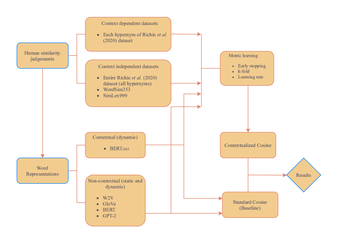
Figure 1: Schematic representation of the experiment leading up to the results in Tables 4 and 5.

3.1 Datasets

For a contextualized assessments of word similarity, we use the dataset of Richie et al. (2020), where 365 participants were asked to judge the similarity between English word-pairs that are co-hyponyms of eight different hypernyms (Table 1). Participants were assigned a specific hypernym and were asked to rate the similarity between each co-hyponym pair from 1 to 7, with the highest rating indicating the words to be maximally similar. The number of annotators varies per hypernym, but each word-pair is rated by around 30 annotators, such that for the largest categories each annotator only saw a fraction of the totality of the word-pairs. As examples from the hypernym ‘Clothing’, the word-pair ‘hat/overalls’ was rated by 32 of the 61 annotators, resulting in an average similarity of 1.469, while ‘coat/gloves’ had an average similarity rating of 3.281 and ‘coat/jacket’ of 6.438, also by 32 annotators. The average similarity was computed for all word-pairs and rescaled to a value between 0 and 1, to be used as the target for supervised learning.

Besides trying to fit a contextualized similarity measure to each hypernym, we also considered the entire all-hypernyms dataset, in order to test whether training on the hypernyms separately would result in a better cosine measure compared with when the hypernym information was disregarded.

To test whether similarity measures can be learned if the similarity of words is not assessed within a specific context, we use the WordSim-353 (WS353) Finkelstein et al. (2001) and part of the SimLex-999 (SL999) Hill et al. (2015) datasets, where the word-pairs bear no specific semantic relation. From the SL999 dataset only the nouns were included, resulting in a dataset of 666 word-pairs. Additionally, we use these datasets to verify whether the similarity metric learned by training on the whole dataset of Richie et al. (2020) can be transferred to other, more general, datasets.

Table 1: Number of words, word-pairs and human annotators per hypernym.

Hypernym	Words	Pairs	Annotators
Birds	30	435	54
Clothing	29	406	61
Professions	28	378	67
Sports	28	378	61
Vehicles	22	231	28
Fruit	21	210	31
Furniture	20	190	33
Vegetables	20	190	30
All	198	2418	365

3.2 Word embeddings

To fine-tune the cosine similarity measure, we start from different pre-trained word representations. We do that for two classes of embeddings, static and dynamic.

Static embeddings were obtained from a pre-trained word2vec (W2V) model Mikolov et al. (2013) and a pre-trained GloVe model Pennington et al. (2014), each used to encode each word in the pair. Dynamic embeddings were obtained from two Transformers-based models, pre-trained BERT Devlin et al. (2019) and GPT-2 models Radford et al. (2019) (see Table 2). Here the representation of each word was taken to be the average representation of sub-word tokens when necessary, excluding the [CLS] and [SEP] tokens.

Representation	Corpus	Corpus size	Dim
word2vec	Google News	100B	300
GloVe	GigaWord Corpus & Wikipedia	6B	200
BERTbase-uncased	BooksCorpus & English Wikipedia	3.3B	768
GPT-2medium	8 million web pages	$\sim$ 40 GB	768

Table 2: Pre-trained embeddings obtained from different source language models, with BERT and GPT-2 implemented using the Huggingface Transformers library.

Hypernym	Context words
Birds	small, migratory, other,
	water, breeding
Clothing	cotton, heavy, outer, winter,
	leather
Professions	health, legal, engineering,
	other, professional
Sports	youth, women, men, ea, boys
Vehicles	military, agricultural, motor,
	recreational, commercial
Fruit	citrus, summer, wild, sweet,
	passion
Furniture	wood, furniture, modern,
	antique, office
Vegetables	some, wild, root, fresh, green

Table 3: Five most likely words for masked token preceding hypernym token using BERT.

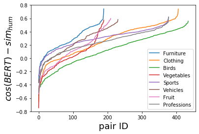
(a)

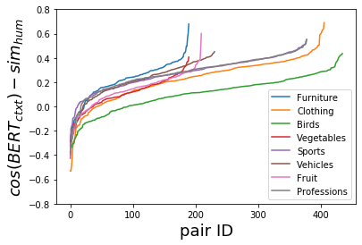
(b)

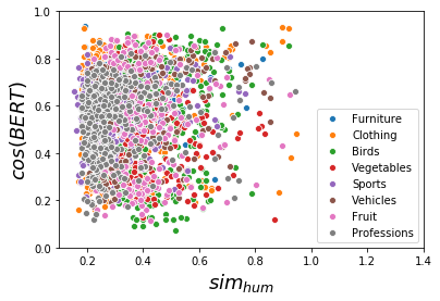
(c)

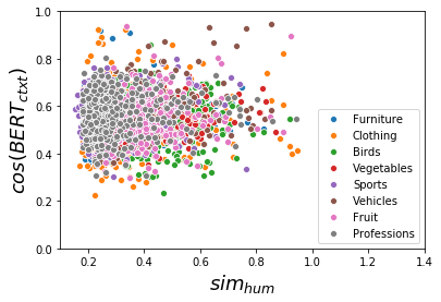
(d)

Figure 2: Distributions of pairwise human similarity judgments $sim_{hum}$ and cosine similarity measures using either BERT representations ($\cos(\text{BERT})$) or contextualized BERT representations ($\cos(\text{BERT}_{ctxt})$). In (a) and (b) the absolute difference of scores, ordered per hypernym, is shown, while (c) and (d) represent the distribution of different similarity scores with respect to each other. Comparing the first two plots we can see a regularization effect by contextualizing the representations, and between the last two plots we can see a clustering effect.

The token representations provided by the BERT model, as a bidirectional dynamic language model, can change depending on the surrounding context tokens. As such, additional contextualized embeddings were retrieved, BERT_ctxt, to test whether performance could be improved relative to the baseline cosine metric by using the hypernym information, as well as when compared with the hypernym cosine metric learned on non-contextualized representations. In this way we test whether leveraging the contextual information intrinsic to this dataset can in itself improve similarity at the baseline level, without the need of further training.

The contextualized vectors of BERT_ctxt were obtained by first having BERT predict the five most likely adjectives that precede each hypernym using ([MASK] <hypernym>), and then using those adjectives to obtain five contextualized embeddings for each co-hyponym, subsequently averaged over. Most of the predicted words were adjectives, and the few cases that were not were filtered out. For instance, for the category ‘Clothing’, the most likely masked tokens were ‘cotton’, ‘heavy’, ‘outer’, ‘winter’ and ‘leather’. The contextualized representation of each hyponyms of ‘Clothing’ was thus calculated as its average representation in the context of each of the adjectives, so that, for instance, for ’coat’ we first obtained its contextualized representation in ‘cotton coat’, ‘heavy coat’, ‘outer coat’, ‘winter coat’, and ‘leather coat’, performing a final averaging. The full list of context words can be found in Table 3. Figs. 2(a) and 2(b) show that this transformation reduces the absolute extreme values of the difference between the values of the standard cosine similarity and the corresponding human similarity assessments, while regularizing the bulk of the differences closer to the desired value of 0. We tested other forms of contextualizing, such as (<hypernym> is/are [MASK]), but the resulting representations did not show as much improvement.

The WS353 and SL999 datasets were only trained with non-contextualized embeddings, since we cannot obtain contextualized embeddings for the nouns in these datasets using the same method. For consistency, the models that were learned with contextualized representations were not tested on these datasets at the final step of our experiment.

3.3 Model

A linear model was implemented on the PyTorch machine learning framework to learn the parameters of $B$, without a bias, such that a word initially represented by $\text{input}_{a}$ is transformed to $\text{input'}_{a}=B\text{input}_{a}$. The forward function of this model takes two inputs and returns

$$\frac{\left(\text{input'}_{a}\right)^{T}\cdot\text{input'}_{b}}{\sqrt{\left(\text{input'}_{a}\right)^{T}\cdot\text{input'}_{1}}\sqrt{\left(\text{input'}_{b}\right)^{T}\cdot\text{input}_{b}}},$$ (7)

where $a$ and $b$ correspond to the indices of the words of a given word-pair.

3.4 Cross-validation

The number of co-hyponyms per hypernym is small when compared with the number of parameters in $B$ to be trained, which depends on the square of the dimension Dim of each representation. To ensure that the models did not overfit, a k-fold cross-validation was used during training Raschka (2015), which divided each dataset in k training sets and non-overlapping development sets. Additionally, early stopping of training was implemented in the event that the validation loss increased for ten consecutive epochs after it dropped below 0.1 Bishop (2006).

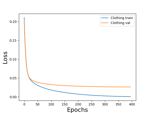
Figure 3: Example of learning curve, showing losses over epochs, from a fold training on the hypernym Clothes on the GloVe embeddings. In this case, training was stopped early at 397 epochs.

3.5 Hyperparameter selection

Per each dataset $h$ (each hypernym, all hypernyms, WS353 or SL999) and learning rate $l_{r}$, k models $B^{h}_{i,l_{r}}$ were trained, with $i\in\{1,...,k\}$ and with k corresponding validation sets $val_{i}$. The training was done using two 16 cores (64 threads) Intel Xeon CPU at 2.1 GHz.

A fixed seed was used to find the best combination of the learning rate $l_{r}$ ($1\times 10^{-5}$, $1\times 10^{-6}$, and $1\times 10^{-7}$) and the number of folds (5, 6 and 7) for the k-fold cross-validation. The regression to the best metric was done using the mean square error loss function and the Adam optimizer. The maximum number of training epochs was set to $500$, as most models converged at that point as per preliminary learning curve inspection (Fig.3). The implementation of early stopping resulted in de facto variation of the number of epochs required to train each model.

(a) Pearson correlations.

Dataset (h)	BERT		BERTctxt		GPT-2		word2vec		GloVe
	Model	Base	Model	Base	Model	Base	Model	Base	Model	Base
Birds	0.311	0.098	0.316	0.042	0.200	-0.023	0.293	0.213	0.215	0.194
Clothing	0.550	0.141	0.515	0.065	0.501	0.349	0.529	0.417	0.574	0.364
Professions	0.501	0.193	0.601	0.073	0.651	0.542	0.635	0.566	0.529	0.529
Sports	0.452	0.175	0.543	0.139	0.556	0.324	0.532	0.418	0.580	0.386
Vehicles	0.496	0.218	0.616	0.123	0.645	0.385	0.738	0.719	0.703	0.567
Fruit	0.315	0.016	0.378	-0.037	0.333	0.203	0.361	0.239	0.571	0.392
Furniture	0.353	-0.018	0.539	-0.035	0.568	0.399	0.368	0.333	0.470	0.462
Vegetables	0.211	-0.059	0.293	-0.044	0.378	0.144	0.577	0.281	0.562	0.290
All hypernyms	0.434	0.100	0.542	0.040	0.508	0.287	0.483	0.400	0.539	0.397
WordSim-353	0.517	0.238	-	-	0.651	0.647	0.637	0.654	0.622	0.568
SimLex-999	0.403	0.161	-	-	0.555	0.504	0.495	0.455	0.510	0.408

(b) Spearman correlations.

Dataset (h)	BERT		BERTctxt		GPT-2		word2vec		GloVe
	Model	Base	Model	Base	Model	Base	Model	Base	Model	Base
Birds	0.260	0.102	0.299	0.052	0.190	-0.054	0.250	0.211	0.238	0.201
Clothing	0.436	0.184	0.467	0.059	0.445	0.276	0.510	0.414	0.513	0.384
Professions	0.501	0.248	0.578	0.170	0.560	0.473	0.518	0.410	0.482	0.486
Sports	0.391	0.174	0.526	0.142	0.540	0.291	0.458	0.339	0.478	0.325
Vehicles	0.518	0.238	0.601	0.056	0.626	0.288	0.709	0.687	0.680	0.596
Fruit	0.265	-0.014	0.333	-0.103	0.365	0.173	0.368	0.277	0.491	0.342
Furniture	0.353	-0.032	0.491	-0.120	0.527	0.393	0.442	0.402	0.464	0.451
Vegetables	0.217	-0.028	0.305	0.015	0.363	0.089	0.587	0.290	0.528	0.228
All hypernyms	0.407	0.111	0.504	0.034	0.504	0.242	0.446	0.379	0.477	0.377
WordSim-353	0.543	0.267	-	-	0.715	0.705	0.675	0.701	0.624	0.579
SimLex-999	0.416	0.180	-	-	0.566	0.513	0.475	0.445	0.500	0.374

Table 4: Best correlation scores between human similarity judgments and similarity scores found by the trained model, compared with baseline cosine metric values of the same hyperparameters. The underlined correlation values are the statistical significant values with a p $<$ 0.05, and the bold values correspond to model correlations that were higher than base correlations.

(a) Pearson correlations.

Dataset (h)	BERT		BERTctxt		GPT-2		W2V		GloVe
	$\%$	$l_{r}$, k	$\%$	$lr$, k	$\%$	$lr$, k	$\%$	$lr$, k	$\%$	$lr$, k
Birds	217	$10^{-6}$,5	652	$10^{-6}$, 5	770	$10^{-5}$, 5	38	$10^{-5}$, 5	11	$10^{-5}$, 7
Clothing	290	$10^{-6}$,5	692	$10^{-6}$, 6	44	$10^{-5}$, 6	27	$10^{-5}$, 7	58	$10^{-6}$, 5
Professions	160	$10^{-6}$, 5	723	$10^{-6}$, 6	20	$10^{-5}$, 5	12	$10^{-5}$, 7	0	$10^{-5}$, 5
Sports	158	$10^{-5}$, 6	291	$10^{-6}$, 6	72	$10^{-5}$, 6	27	$10^{-5}$, 6	50	$10^{-6}$, 7
Vehicles	128	$10^{-6}$, 6	401	$10^{-5}$, 7	68	$10^{-5}$, 5	3	$10^{-5}$, 5	24	$10^{-6}$, 6
Fruit	1869	$10^{-5}$, 7	922	$10^{-6}$, 6	64	$10^{-5}$, 7	51	$10^{-6}$, 5	46	$10^{-7}$, 7
Furniture	1861	$10^{-5}$, 7	1440	$10^{-6}$, 6	42	$10^{-5}$, 7	11	$10^{-5}$, 6	2	$10^{-5}$, 6
Vegetables	258	$10^{-5}$, 7	566	$10^{-6}$, 6	163	$10^{-5}$, 5	105	$10^{-6}$, 7	94	$10^{-6}$, 5
All	334	$10^{-5}$, 5	1255	$10^{-6}$, 7	77	$10^{-5}$, 6	21	$10^{-5}$, 6	36	$10^{-7}$, 6
WordSim-353	117	$10^{-6}$, 7	-	-	1	$10^{-5}$, 7	-3	$10^{-5}$, 6	10	$10^{-5}$, 5
SimLex-999	150	$10^{-6}$, 7	-	-	10	$10^{-5}$, 6	9	$10^{-5}$, 6	25	$10^{-6}$, 5

(b) Spearman correlations.

Dataset (h)	BERT		BERTctxt		GPT-2		W2V		GloVe
	$\%$	$lr$, k	$\%$	$lr$, k	$\%$	$lr$, k	$\%$	$lr$, k	$\%$	$lr$, k
Birds	155	$10^{-6}$, 5	475	$10^{-6}$, 5	252	$10^{-5}$, 7	18	$10^{-5}$, 5	18	$10^{-7}$, 5
Clothing	137	$10^{-6}$, 5	692	$10^{-6}$, 6	61	$10^{-5}$, 7	23	$10^{-5}$, 7	34	$10^{-6}$, 5
Professions	102	$10^{-6}$, 7	240	$10^{-6}$, 5	18	$10^{-5}$, 5	26	$10^{-5}$, 7	-1	$10^{-7}$, 6
Sports	125	$10^{-5}$, 6	270	$10^{-6}$, 6	86	$10^{-5}$, 6	35	$10^{-5}$, 6	47	$10^{-6}$, 6
Vehicles	118	$10^{-6}$, 6	973	$10^{-6}$, 6	117	$10^{-5}$, 7	3	$10^{-5}$, 5	14	$10^{-6}$, 6
Fruit	1793	$10^{-6}$, 7	223	$10^{-6}$, 6	111	$10^{-5}$, 6	33	$10^{-6}$, 6	44	$10^{-7}$, 7
Furniture	1003	$10^{-6}$, 6	309	$10^{-6}$, 5	34	$10^{-5}$, 5	10	$10^{-5}$, 6	3	$10^{-6}$, 7
Vegetables	675	$10^{-5}$, 7	1933	$10^{-6}$, 6	308	$10^{-5}$, 5	102	$10^{-6}$, 7	132	$10^{-6}$, 5
All hypernyms	267	$10^{-5}$, 5	1382	$10^{-6}$, 7	108	$10^{-5}$, 6	18	$10^{-5}$, 6	27	$10^{-6}$, 5
WordSim-353	103	$10^{-6}$, 5	-	-	1	$10^{-5}$, 7	-4	$10^{-6}$, 5	8	$10^{-5}$, 5
SimLex-999	131	$10^{-6}$, 7	-	-	10	$10^{-5}$, 6	7	$10^{-5}$, 6	34	$10^{-6}$, 5

Table 5: Change ($\%$) in correlation from Table 4, given by $(|\text{Model}|-|\text{Base}|)/|\text{Base}|$, at corresponding best hyperparameters ($lr$, k). Values in bold indicate the highest increase on a given dataset.

3.6 Testing the model

Each one of the $B^{h}_{i,l_{r}}$ models was tested on the corresponding holdout validation set $val_{i}$, resulting in two correlation scores between the models’ predicted similarity scores and the human judgment scores: a Pearson correlation score $r^{h}_{i,l_{r}}(val^{h}_{i})$ and a Spearman correlation score $\rho^{h}_{i,l_{r}}(val^{h}_{i})$. A final score per k and $l_{r}$ was calculated using the average performance on the validation sets as

$$r^{h}_{k,l_{r}}=\frac{1}{k}\sum_{i=1}^{k}r^{h}_{i,l_{r}}(val^{h}_{i}),$$ (8)

$$\rho^{h}_{k,l_{r}}=\frac{1}{k}\sum_{i=1}^{k}\rho^{h}_{i,l_{r}}(val^{h}_{i}).$$ (9)

The baseline results were obtained in a similar form, but with the model $B^{std}$ corresponding to the identity matrix, returning the standard cosine similarity rating as

$$r^{h,std}_{k}=\frac{1}{k}\sum_{i=1}^{k}r^{std}(val^{h}_{i}),$$ (10)

$$\rho^{h,std}_{k}=\frac{1}{k}\sum_{i=1}^{k}\rho^{std}(val^{h}_{i}).$$ (11)

The model results shown in Table 4 correspond to the best correlation values obtained using Eqs. (8) and (9), with the baselines given as in Eqs. (10) and (11). The hyperparameters corresponding to the best results can be found in Table 5, along with the relative change in correlation performance. As the seed was fixed, the differences in performance achieved by models trained on each hypernym and on all-hypernyms of the contextualized dataset were not due to randomization errors. The final correlation per fold on the entire all-hypernyms dataset was found by first calculating the correlation per hypernym and then averaging over all eight hypernyms.

To test the transferability of the metric learned on the all-hypernyms dataset to other datasets, the model that returned the best correlation scores on the validation datasets of the all-hypernyms dataset was tested on the entire WS353 and SL999 datasets. As the best performing model consists in fact of k models, each one of these was tested on the entire datasets, as

$$r^{h,test}_{k,l_{r}}=\frac{1}{k}\sum_{i=1}^{k}r^{All-hyp}_{i,l_{r}}(test^{h}),$$ (12)

$$\rho^{h,test}_{k,l_{r}}=\frac{1}{k}\sum_{i=1}^{k}\rho^{All-hyp}_{i,l_{r}}(test^{h}),$$ (13)

with $h\in\{\text{WS353},\text{SL999}\}$.

The baselines for these results were obtained by applying $B^{std}$ to the entire WS353 and SL999 datasets as

$$r^{h,std}=r^{std}(test^{h}),$$ (14)

$$\rho^{h,std}=\rho^{std}(test^{h}).$$ (15)

As the correlation functions are not linear, the results from Eqs. (10) and (11) for the WS353 and SL999 datasets are expected to differ from those obtained using Eqs. (14) and (15) for the same datasets.

4 Results

The validation results on Table 4 show consistent improvements over the baselines, with statistical significance. This confirms that the modification introduced to the cosine measure worked in a principled way, and consistent with the results found by Richie and Bhatia (2021). On the individual hypernym datasets, ‘Vehicles’ showed the best correlations, except for the Pearson correlation in GPT-2, in spite of not being the largest hypernym dataset. On the contrary, the smallest categories showed the lowest correlations. In general, the relative performance of hypernyms according to the baselines extends to the model correlations, although with better performance. With some exceptions, mainly in the ‘Birds’ hypernym, the best performing representation was GPT-2, followed by W2V, but the relative increase as shown in Table 5 was clearly superior for the dynamic representations. An important observation that we make is that the model trained on all hypernyms had a better performance than the average performance on the individual hypernyms. As the seed was fixed, this means that the performance on the hypernym-specific validation sets increased if at training time the models saw more examples, from different categories, indicating that a similarity relationship was learned and transferred across different contexts. Improvements over baseline also took place if a metric was learned on datasets where the word pairs did not share a context, as was the case with WS353 and SL999, but the percentual increase was lower, as seen in Table 5.

Comparing the results of BERT contextualized and non-contextualized, the baseline values of the contextualized representations were worse than those obtained with the contextualized embeddings, although without statistical significance, while the improvement after training was consistently better and significant for all datasets with the contextualized representations. Figs. 2(c) and 2(d), show that the distribution of points using the contextualized embeddings is more concentrated and collinear, making it more likely that a metric that acts in the same way for all points in the dataset will rotate and rescale them into a positive correlation. The percentual increases also show that BERT contextualized had the greatest increases from before to after training, suggesting that there was a cumulative effect in considering the context both in the representations and in the similarity measure.

Table 4 shows the results of applying the best model learned on all hypernyms to the WS353 and SL999 datasets. The baseline values for the static representations are comparable with the existing literature Toshevska et al. (2020). We see that our model was capable of improving on the correlation scores on the datasets, for some representations. Although the improvements did not happen across the board, they show clear evidence that the notion of similarity in the form of a modified cosine measure can be learned in one dataset and applied with positive results to an independent dataset.

[t]

		Pearson		Spearman
		WS353	SL999	WS353	SL999
BERT	Model	0.487	0.375	0.519	0.384
	Base	0.239	0.151	0.267	0.172
GPT-2	Model	0.635	0.507	0.676	0.513
	Base	0.647	0.504	0.709	0.520
W2V	Model	0.613	0.472	0.632	0.457
	Base	0.653	0.460	0.700	0.452
GloVe	Model	0.593	0.431	0.558	0.392
	Base	0.578	0.408	0.578	0.376
SOTA		0.704	0.658	0.828	0.76

Best model trained on all hypernyms, tested on SimLex-999 and WordSim-353 datasets. Bold values indicate correlation scores above baseline, and underlining indicates statistical significance. State of the art from Recski et al. (2016); Dobó and Csirik (2020); Speer et al. (2017); Banjade et al. (2015).

5 Conclusion and Outlook

In this paper we tested whether a contextualized notion of cosine similarity could be learned, improving the similarity not only of the results for the datasets where it was learned, but of unrelated similarities. We showed that this metric improved the correlations above baseline, and that, when learned on a contextualized similarity dataset, it had an advantage when compared to one learned on a dataset with unrelated word-pairs. We furthermore showed that this framework has the potential to generalize the notion of similarity to word-pairs it has not seen during training. An important future research line towards interpretability consists in understanding the properties of the metrics that yielded the best results, particularly in identifying the distinctive features of the best metrics, such as their eigensystems. Other further directions include applying these metrics to distributional compositional contractions, including with dependency enhancements Kogkalidis et al. (2019), testing this framework on larger contextualized datasets and trying out more complex, non-linear, metric forms.

References

- Abbaszadeh et al. (2021) Mina Abbaszadeh, S Shahin Mousavi, and Vahid Salari. 2021. Parametrized quantum circuits of synonymous sentences in quantum natural language processing. arXiv preprint arXiv:2102.02204.
- Axler (1997) Sheldon Jay Axler. 1997. Linear algebra done right. Springer.
- Banjade et al. (2015) Rajendra Banjade, Nabin Maharjan, Nobal B Niraula, Vasile Rus, and Dipesh Gautam. 2015. Lemon and tea are not similar: Measuring word-to-word similarity by combining different methods. In International conference on intelligent text processing and computational linguistics, pages 335–346.
- Baroni et al. (2014) Marco Baroni, Raffaella Bernardi, and Roberto Zamparelli. 2014. Frege in space: A program for composition distributional semantics. In Linguistic Issues in Language Technology, Volume 9, 2014-Perspectives on Semantic Representations for Textual Inference.
- Barsalou (1982) Lawrence W Barsalou. 1982. Context-independent and context-dependent information in concepts. Memory & cognition, 10(1):82–93.
- Bender et al. (2021) Emily M Bender, Timnit Gebru, Angelina McMillan-Major, and Shmargaret Shmitchell. 2021. On the dangers of stochastic parrots: Can language models be too big? In Proceedings of the 2021 ACM Conference on Fairness, Accountability, and Transparency (ACM FAccT ‘21), pages 610–623.
- Bishop (2006) Christopher M Bishop. 2006. Pattern recognition and machine learning. Springer.
- Coecke and Clark (2010) M Sadrzadeh B Coecke and S Clark. 2010. Mathematical foundations for a compositional distributed model of meaning. Lambek Festschirft‚ Linguistic Analysis, 36(1-4):345–384.
- Correia et al. (2020) Adriana D Correia, Michael Moortgat, and Henk TC Stoof. 2020. Density matrices with metric for derivational ambiguity. Journal of Applied Logics, 2631(5):795.
- Devlin et al. (2019) Jacob Devlin, Ming-Wei Chang, Kenton Lee, and Kristina Toutanova. 2019. Bert: Pre-training of deep bidirectional transformers for language understanding. In Proceedings of the 2019 Conference of the North American Chapter of the Association for Computational Linguistics (NAACL ‘19), pages 4171–4186.
- Dobó and Csirik (2020) András Dobó and János Csirik. 2020. A comprehensive study of the parameters in the creation and comparison of feature vectors in distributional semantic models. Journal of Quantitative Linguistics, 27(3):244–271.
- Finkelstein et al. (2001) Lev Finkelstein, Evgeniy Gabrilovich, Yossi Matias, Ehud Rivlin, Zach Solan, Gadi Wolfman, and Eytan Ruppin. 2001. Placing search in context: The concept revisited. In Proceedings of the 10th International Conference on World Wide Web (WWW ‘01), pages 406–414.
- Goldstone et al. (1997) Robert L Goldstone, Douglas L Medin, and Jamin Halberstadt. 1997. Similarity in context. Memory & Cognition, 25(2):237–255.
- Grefenstette and Sadrzadeh (2011a) Edward Grefenstette and Mehrnoosh Sadrzadeh. 2011a. Experimental support for a categorical compositional distributional model of meaning. In Proceedings of the 2011 Conference on Empirical Methods in Natural Language Processing (EMNLP ‘11), page 1394–1404.
- Grefenstette and Sadrzadeh (2011b) Edward Grefenstette and Mehrnoosh Sadrzadeh. 2011b. Experimenting with transitive verbs in a DisCoCat. In Proceedings of the 2011 Workshop on GEometrical Models of Natural Language Semantics (GEMS ‘11), pages 62–66.
- Hewitt and Manning (2019) John Hewitt and Christopher D Manning. 2019. A structural probe for finding syntax in word representations. In Proceedings of the 2019 Conference of the North American Chapter of the Association for Computational Linguistics (NAACL ‘19), pages 4129–4138.
- Hill et al. (2015) Felix Hill, Roi Reichart, and Anna Korhonen. 2015. Simlex-999: Evaluating semantic models with (genuine) similarity estimation. Computational Linguistics, 41(4):665–695.
- Kogkalidis et al. (2019) Konstantinos Kogkalidis, Michael Moortgat, and Tejaswini Deoskar. 2019. Constructive type-logical supertagging with self-attention networks. In Proceedings of the 4th Workshop on Representation Learning for NLP (RepL4NLP ‘19), pages 113–123.
- Kulis et al. (2013) Brian Kulis et al. 2013. Metric learning: A survey. Foundations and Trends® in Machine Learning, 5(4):287–364.
- Levart (2011) Borut Levart. 2011. Triangles on a sphere. Wolfram Demonstrations Project.
- Medin et al. (1993) Douglas L Medin, Robert L Goldstone, and Dedre Gentner. 1993. Respects for similarity. Psychological review, 100(2):254.
- Mikolov et al. (2013) Tomas Mikolov, Ilya Sutskever, Kai Chen, Greg Corrado, and Jeffrey Dean. 2013. Distributed representations of words and phrases and their compositionality. In Proceedings of the 26th International Conference on Neural Information Processing Systems (NIPS ‘13), pages 3111–3119.
- Milajevs et al. (2014) Dmitrijs Milajevs, Dimitri Kartsaklis, Mehrnoosh Sadrzadeh, and Matthew Purver. 2014. Evaluating neural word representations in tensor-based compositional settings. In Proceedings of the 2014 Conference on Empirical Methods in Natural Language Processing (EMNLP ‘14), pages 708–719.
- Paperno et al. (2014) Denis Paperno, Marco Baroni, et al. 2014. A practical and linguistically-motivated approach to compositional distributional semantics. In Proceedings of the 52nd Annual Meeting of the Association for Computational Linguistics (ACL ‘14), pages 90–99.
- Pennington et al. (2014) Jeffrey Pennington, Richard Socher, and Christopher D Manning. 2014. Glove: Global vectors for word representation. In Proceedings of the 2014 Conference on Empirical Methods in Natural Language Processing (EMNLP ‘14), pages 1532–1543.
- Radford et al. (2019) Alec Radford, Jeffrey Wu, Rewon Child, David Luan, Dario Amodei, and Ilya Sutskever. 2019. Language models are unsupervised multitask learners. OpenAI blog, 1(8):9.
- Raschka (2015) Sebastian Raschka. 2015. Python machine learning. Packt publishing.
- Recski et al. (2016) Gábor Recski, Eszter Iklódi, Katalin Pajkossy, and András Kornai. 2016. Measuring semantic similarity of words using concept networks. In Proceedings of the 1st Workshop on Representation Learning for NLP (RepL4NLP ‘16), pages 193–200.
- Richie and Bhatia (2021) Russell Richie and Sudeep Bhatia. 2021. Similarity judgment within and across categories: A comprehensive model comparison. Cognitive Science, 45(8):e13030.
- Richie et al. (2020) Russell Richie, Bryan White, Sudeep Bhatia, and Michael C Hout. 2020. The spatial arrangement method of measuring similarity can capture high-dimensional semantic structures. Behavior research methods, 52(5):1906–1928.
- Salton and McGill (1983) Gerard Salton and Michael J McGill. 1983. Introduction to modern information retrieval. McGraw Hill.
- Schwarz et al. (2017) Mykhaylo Schwarz, Mykhaylo Lobur, and Yuriy Stekh. 2017. Analysis of the effectiveness of similarity measures for recommender systems. In Porceedings of the 14th International Conference The Experience of Designing and Application of CAD Systems in Microelectronics (CADSM ‘17), pages 275–277.
- Sidorov et al. (2014) Grigori Sidorov, Alexander Gelbukh, Helena Gómez-Adorno, and David Pinto. 2014. Soft similarity and soft cosine measure: Similarity of features in vector space model. Computación y Sistemas, 18(3):491–504.
- Speer et al. (2017) Robyn Speer, Joshua Chin, and Catherine Havasi. 2017. Conceptnet 5.5: An open multilingual graph of general knowledge. In Proceedings of the 31st AAAI Conference on Artificial Intelligence (AAAI ‘17), pages 4444–4451.
- Toshevska et al. (2020) Martina Toshevska, Frosina Stojanovska, and Jovan Kalajdjieski. 2020. Comparative analysis of word embeddings for capturing word similarities. arXiv preprint arXiv:2005.03812.
- Tversky (1977) Amos Tversky. 1977. Features of similarity. Psychological review, 84(4):327.
- Wald (2010) Robert M Wald. 2010. General relativity. University of Chicago Press.
- Wijnholds and Sadrzadeh (2019) Gijs Wijnholds and Mehrnoosh Sadrzadeh. 2019. Evaluating composition models for verb phrase elliptical sentence embeddings. In Proceedings of the 2019 Conference of the North American Chapter of the Association for Computational Linguistics (NAACL ‘19), pages 261–271.
- Witten et al. (2005) Ian H Witten, Eibe Frank, Mark A Hall, and CJ Pal. 2005. Data Mining: Practical machine learning tools and techniques. Elsevier.