Characterization of planar symmetric central configurations of four bodies, models, and an application

Abstract

We overview angle-based models to study planar symmetric central configurations of four bodies. We present models to determine the masses given the shape of the configuration and the shape-type of the configuration given the masses. We also describe a diagram-based method for the counting of the shape-types in the case of the concave configurations. As an application, we determine planar symmetric central configurations containing bodies of Earth’s and Moon’s masses.

Keywords: four-body problem, central configurations

I Introduction

The Newtonian n-body problem is a fundamental problem of celestial mechanics. We study the motion of $n$ point-like bodies interacting with each other according to the Newtonian law of gravity. Given a set of point-like bodies with masses $m_{i}$ and barycentric position vectors $\bm{r_{i}}$, the equations of motion take the form

$$m_{i}\bm{\ddot{r_{i}}}=k^{2}\sum_{j\neq i}\frac{m_{i}m_{j}}{r_{ij}^{3}}(\bm{r_{j}}-\bm{r_{i}})\quad 1\leq i\leq n,$$ (1)

where $k$ is the Gaussian constant of gravity, and $r_{ij}=|\bm{r_{i}}-\bm{r_{j}}|$ denotes the distance between the $i$th and $j$th bodies.

Newton solved Eqs. (1) for two bodies ($n=2$). However, the complete set of solutions of Eqs. (1) for more than two bodies ($n>2$) is yet to be determined. So the study of different particular solution subclasses is crucial. Central configurations represent one such solution subclass. In central configurations, the resulting forces on all bodies point towards the center of mass of the configuration. Thus the accelerations are

$$\bm{\ddot{r_{i}}}=-\lambda\bm{r_{i}}\quad 1\leq i\leq n,$$ (2)

where $\lambda>0$ is the same for all bodies. Accordingly, the equations of condition for central configurations with Newtonian accelerations take the from

$$\sum_{j\neq i}\frac{m_{j}}{r_{ij}^{3}}(\bm{r_{j}}-\bm{r_{i}})=\Lambda\bm{r_{i}}\quad 1\leq i\leq n,$$ (3)

where $\Lambda=-\lambda/k^{2}$.

Characterizing central configurations is an important task from both a mathematical and physical point of view. For example, from a mathematical perspective, central configurations have a pivotal role in the topology of the n-body problem (see Ref. [8]). From a physical viewpoint, a system of bodies colliding or expanding according to a physical law, asymptotically tends to a central configuration (see Ref. [7]). The study of the central configurations is also extremely difficult. Questions about the central configurations even appeared in the lists of some authors’ challenging problems for the 21st century, for example papers [9] and [1]. The publication of these lists led to intensive studies of the central configurations around the turn of the 21st century. Despite the efforts, many questions are still unanswered for configurations containing four or more bodies ($n\geq 4$). For reference, central configurations formed by three bodies ($n=3$) were determined by Euler and Lagrange (see Refs. [4] and [5]) already in the 18th century.

In this paper, we study the planar symmetric central configurations of four bodies (from now on abbreviated as PSCCFB for simplicity). In Sect. II, we summarize the models and methods presented in studies [3] and [2] that are suitable to determine the masses of the bodies of the system based on the shape of the configuration, and the number of the types of the configurations based on the masses. The methods presented in [2] determine the number of the types of the configurations knowing the placements of the masses within the configuration. Here we determine that number without the knowledge of the placements of the masses in the configuration. As an application, in Sect. III, we characterize all possible types of the PSCCFB where some of the bodies have Earth’s and Moon’s masses.

II Angle-based models of the PSCCFB

The term central configurations was introduced by Laplace in [6] while he was examining the Lagrangian solutions of the three-body problem. According to his mode of discussion, giving a solution for the problem consists of determining all possible geometrical configurations and mass arrangements for a predetermined set of masses (this is the so-called direct problem). The inverse problem is a reverse procedure, where one determines the masses for configurations with given shapes.

Determining all the central configurations with a set number of bodies with predetermined masses seems hopeless because these types of systems are self-similar, i.e., invariant under rotation, translation, and dilation. A more reasonable task is to use the self-similarity property to define equivalence classes and count them. Though, counting these classes still proves to be an intricate task partly because, in some cases, they distinguish between configurations with the same shape but different labelling of the bodies. Thus it is more convenient to count affine classes, which are the same as equivalence ones but without labelling of the bodies. In this paper, we define the number of central configurations as the number of affine classes.

In the following subsections, we first briefly overview our previous studies on the inverse problem (Sect. II.1), and then utilize our results to solve the direct problem (Sect. II.2).

II.1 Overview of the inverse problem

In this subsection, we sum up our results on the inverse problem described in [3] and [2].

In [2] we proved that in the PSCCFB there is at least one axis of symmetry. Thus to solve the inverse problem, one needs to study two cases:

1. when there are no bodies on the axis of symmetry,

2. when there are two bodies on the axis of symmetry.

A full description of Case (a) is given in [2], while that of Case (b) in [3].

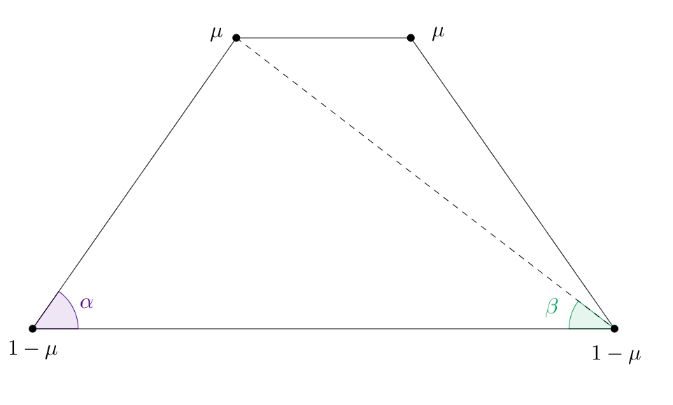
Figure 1: Isosceles trapezoid type configuration. Symmetric quadrilateral without a body on its axis of symmetry.

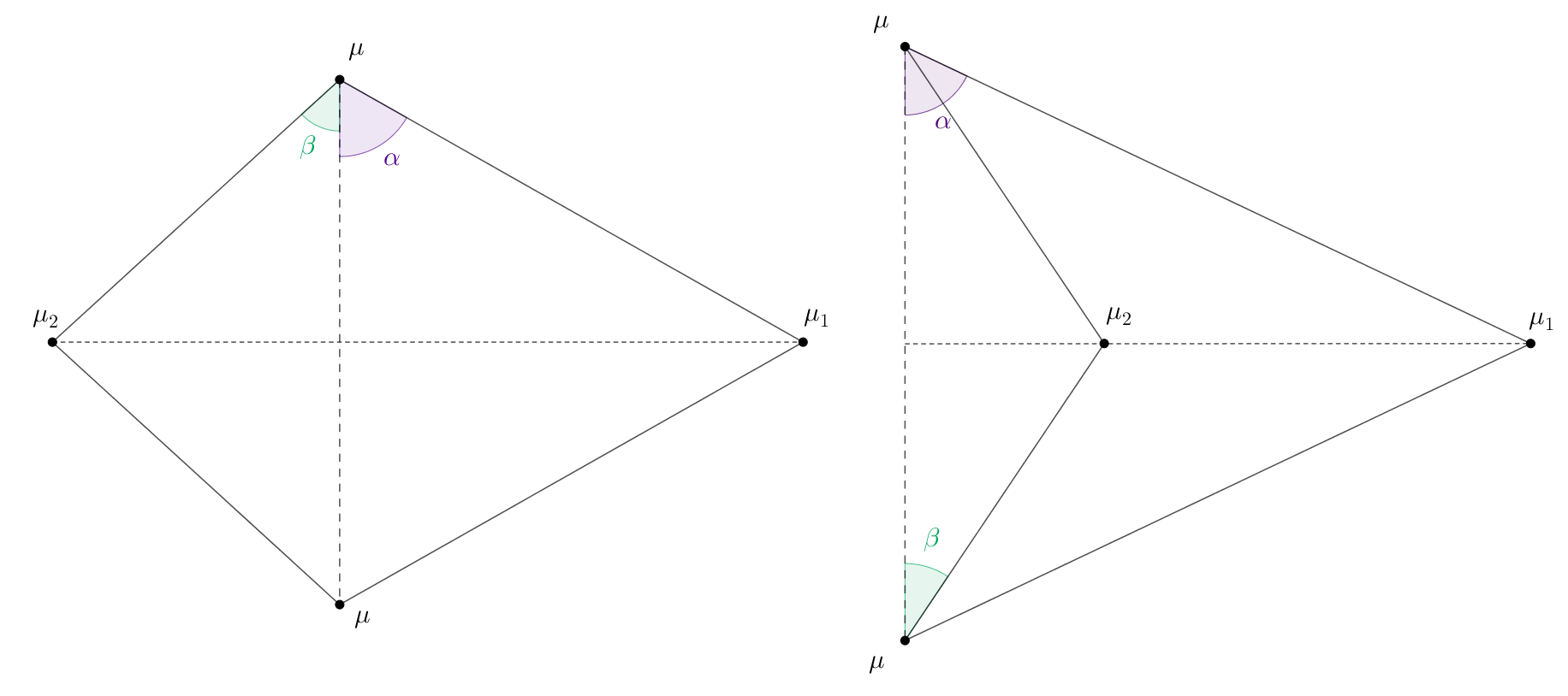
Figure 2: Configuration types with two bodies on the axis of symmetry. Convex composition on the left side, while concave on the right side.

A configuration in Case (a) takes an isosceles trapezoidal form (see Fig. 2). The bodies that are reflections of each other (with respect to the axis of symmetry) have identical masses. The shape of the configuration uniquely determines the mass arrangement. To calculate the non-dimensional mass $\mu$ (see Fig. 2), one needs to solve the following system of Eqs. (see Ref. [2]):

$$\begin{split}&[\sin^{3}\beta-\sin^{3}(\alpha+\beta)][\sin^{3}\alpha-\sin^{3}(\alpha-\beta)]+[\sin^{3}\alpha-\sin^{3}(\alpha+\beta)][\sin^{3}\beta-\sin^{3}(\alpha-\beta)]=0,\\ &\mu=\frac{1}{1+\displaystyle{\frac{\sin^{2}(\alpha+\beta)}{\sin^{2}(\alpha-\beta)}\cdot\frac{\sin^{3}\alpha-\sin^{3}(\alpha-\beta)}{\sin^{3}\alpha-\sin^{3}(\alpha+\beta)}}}.\end{split}$$ (4)

Taking into account the geometrical restrictions ($0^{\circ}<\beta<\alpha\leq 90^{\circ}$), the first equation establishes a one-to-one correspondence between the angles $\alpha$ and $\beta$. So just one angle is enough to define the shape of the configuration. The mass $\mu$ can be determined from the second equation of (4), after substituting there the solutions $\alpha$ and $\beta$ of the first equation.

Configurations in Case (b) take convex or concave deltoid shapes (see Fig. 2). The bodies separated by the axis of symmetry have the same mass. In this case, the shape of the configurations also uniquely determines the mass arrangement. Using the notations from Fig. 2, the explicit formulas for the non-dimensional masses $\mu_{1}$, $\mu_{2}$ and $\mu$ are (see Ref. [3]):

$$\mu_{1}=\frac{b_{0}(b_{1}+a_{0}-b_{0})}{a_{0}b_{1}+a_{1}b_{0}-a_{1}b_{1}},\quad\mu_{2}=\frac{a_{0}(a_{1}+b_{0}-a_{0})}{a_{0}b_{1}+a_{1}b_{0}-a_{1}b_{1}},\quad\mu=\frac{1}{2}(1-\mu_{1}-\mu_{2}).$$ (5)

The coefficients $a_{0}$, $a_{1}$, $b_{0}$ and $b_{1}$ are trigonometric polynomials of the angles $\alpha$ and $\beta$ (see Appendix A). Beside the geometrical restriction on the angles ($0^{\circ}<\beta\leq\alpha<90^{\circ}$), there are restrictions on the masses as well ($0\leq\mu_{1},\mu_{2},\mu\leq 1$ and $\mu_{1}+\mu_{2}+2\mu=1$). For acceptable solutions, these restrictions define so-called admissible regions on the parameter space (see Figs. 4 and 4). Any pairs of the angles $\alpha$ and $\beta$ from the blue regions of Fig. 4 or 4 result in convex or concave configurations, respectively, with corresponding masses given by Eqs. (5).

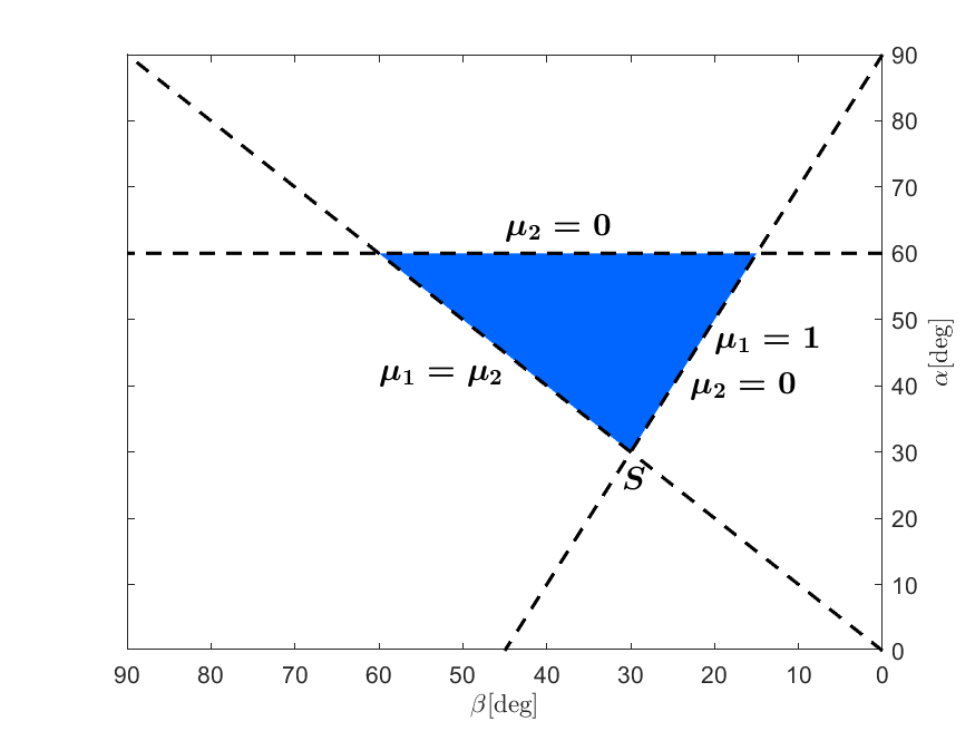
Figure 3: The blue area describes the domain of parameters that lead to acceptable convex solutions (if $\mu_{2}\leq\mu_{1}$). $S$ is a singular point, where the mass functions given by Eqs. (5) are undefined, instead $\mu_{1}+\mu_{2}=1$ holds with arbitrary masses.

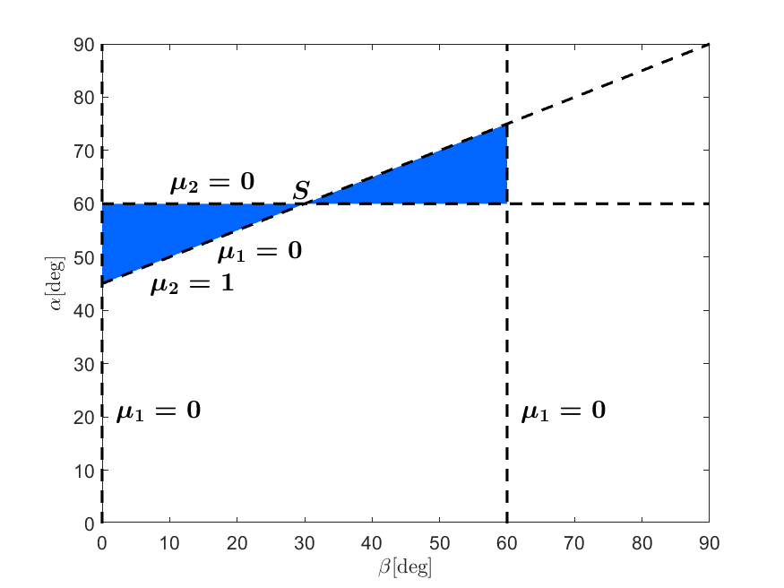
Figure 4: The blue triangle-shaped areas describe the domains of parameters that lead to acceptable concave solutions. On the left are the first, on the right are the second case solutions. $S$ is a singular point, where the mass functions given by Eqs. (5) are undefined, instead $3\mu_{1}+\mu_{2}=1$ holds with arbitrary masses.

Note that the square configuration with four equal masses is the only common solution of Cases (a) and (b).

As a summary of this subsection, we emphasize that the shape of the configurations uniquely determines their mass arrangement. In the isosceles trapezoid case, solving Eqs. (4) will deliver the mass arrangement. Eqs. (5) provide explicit formulae for calculating the masses of the deltoid-type central configurations.

II.2 The direct problem

In this subsection, we describe methods that are suitable to solve the direct problem of the PSCCFB, utilizing the results on the inverse problem presented in Sect. II.1.

Generally, studying the direct problem of central configurations of four bodies, a set of four positive values, representing the masses, is a priori given. In the problem of the PSCCFB, there are some restrictions on the masses. In Case (a), there are two pairs of equal masses, while in Case (b) there is at least one such pair (see Figs. 2 and 2).

Initially, there is no condition on the placement of the masses within the configurations. However, Eqs. (4) and (5) determine the masses at a specific position within the configuration for it to be central (see Figs. 2 and 2). So using these formulae to calculate all possible solutions, this place-specific feature needs to be considered.

The set of masses for Case (a) consists of two pairs of equal masses. Thus the non-dimensional parameter $\mu$ describes the whole mass composition of the configuration (see Fig. 2). In this case, the first of Eqs. (4) establishes a one-to-one correspondence between the angles $\alpha$ and $\beta$, similarly, the second of Eqs. (4) between $\mu$ and the angle pairs $(\alpha,\beta)$. So Eqs. (4) has a unique solution. It can be determined knowing just one of the three parameters ($\mu$, $\alpha$ or $\beta$). So in Case (a), the set of masses of the configuration uniquely determines its shape and vice versa.

Case (b) involves convex and concave configurations (see Fig. 2), each type having a different set of coefficients for the formulae (5). The set of masses contains maximum three different values because the bodies separated by the axis of symmetry are equal. So knowing two of the parameters $\mu_{1}$, $\mu_{2}$ and $\mu$ (see Fig. 2) defines the mass composition of the configuration.

In [2], we have shown that there exists a unique convex configuration for each pair of the mass parameters $\mu_{1}$ and $\mu_{2}$, satisfying $\mu_{1}\geq\mu_{2}$. This condition excludes duplicated solutions due to the $180^{\circ}$ rotational symmetry around the center of mass of the system.

In [2], we have also demonstrated that there exist between 0 and 2 concave type configurations for each pair of $\mu_{1}$ and $\mu_{2}$, depending on their values. In the concave case, there is no restriction for the masses with respect to their relative magnitude. Thus their values can be interchanged. In [2], we studied the concave configurations considering $\mu_{1}$ and $\mu_{2}$ as place-specific mass parameters on the axis of symmetry, taking $\mu_{1}$ as the outer mass and $\mu_{2}$ as the inner one (see the right panel of Fig. 2). Here we consider the solutions of the concave case when the values of the mass parameters are interchangeable. Thus let $m_{1}$ and $m_{2}$ be place-independent mass values, and we look for solutions when $\mu_{1}=m_{1}$, $\mu_{2}=m_{2}$, and $\mu_{1}=m_{2}$, $\mu_{2}=m_{1}$, where $\mu_{1}$ and $\mu_{2}$ are expressions given by Eqs. (5). This problem is described in a general way by the following system of non-linear equations:

$$\begin{split}\mu_{1}(\alpha,\beta)&=m_{i},\\ \mu_{2}(\alpha,\beta)&=m_{j},\end{split}$$ (6)

where $i,j\in\{1,2\}$, $i\neq j$, $\mu_{1}$ and $\mu_{2}$ are expressions given by Eqs. (5), and the angles $\alpha$ and $\beta$ are from within the blue regions in Fig. 4.

In [2], we describe a method for solving the system of Eqs. (6). In the concave case, it begins with calculating the pairs of angle parameters $(\alpha,\beta)$ for which the second equation $\mu_{2}(\alpha,\beta)=m_{j}$ of Eqs. (6) is satisfied. These pairs describe a continuous curve in the admissible angle domain (for examples of such curves see Fig. 14 in 2). Calculating $\mu_{1}$ along this curve will lead to a characteristic curve $\mu_{1}(\mu_{2}(\alpha,\beta)=m_{j})$. Fig. 5 shows such characteristic curves for several values of $m_{j}$. Projecting this $\mu_{1}(\mu_{2}(\alpha,\beta)=m_{j})$ curve onto the plane $(\alpha,\mu_{1})$, its intersection(s) with the line $\mu_{1}=m_{i}$ will provide the solution of Eqs. (6).

On the admissible angle domains (see Fig. 4), the $\mu_{1}(\mu_{2}(\alpha,\beta)=c)$ function changes its monotonicity once (see Fig. 5) at a $M_{1}(\mu_{2}(\alpha,\beta)=c)$ maximum value, where $0\leq c\leq 1$ is a constant. The parameters $(\alpha,\beta,\mu_{1},\mu_{2})$ of the $M_{1}(\mu_{2})$ peak values fulfill the following equation (see Ref. [2]):

$$r\det(J_{qp}(\alpha,\beta))-p\det(J_{qr}(\alpha,\beta))-q\det(J_{rp}(\alpha,\beta))=0,$$ (7)

where $\mu_{1}=q/r$, $\mu_{2}=p/r$ and

$$J_{fg}(\alpha,\beta)=\begin{pmatrix}\frac{\partial f}{\partial\alpha}&\frac{\partial f}{\partial\beta}\\ \frac{\partial g}{\partial\alpha}&\frac{\partial g}{\partial\beta}\end{pmatrix}$$

is the Jacobian matrix and $\det$ stands for the determinant. Fig. 6 shows the curve $M_{1}(\mu_{2})$ on the plane $(\mu_{2},\mu_{1})$. Admissible values of $\mu_{1}$ and $\mu_{2}$ are below the line $\mu_{1}+\mu_{2}=1$, however, mass values only on and below the curve $M_{1}(\mu_{2})$ lead to concave central configurations ($1$ or $2$ solutions, respectively). On the plane $(\mu_{2},\mu_{1})$ the curve $M_{1}(\mu_{2})$ can be approximated by the following function:

$$M_{1}(\mu_{2})=\begin{cases}0.08258\cdot e^{-25.73\mu_{2}}+0.3402\cdot e^{-1.227\mu_{2}},&\mbox{if }0\leq\mu_{2}<0.25034,\\ -0.03846\cdot\mu_{2}^{2}-0.2859\cdot\mu_{2}+0.3241,&\mbox{if }0.25034\leq\mu_{2}\leq 1.\end{cases}$$ (8)

The average precision of the functions (8) is $1.88\cdot 10^{-5}$. The meaning of the critical value $\mu_{2}=0.25034$ in (8) is explained later.

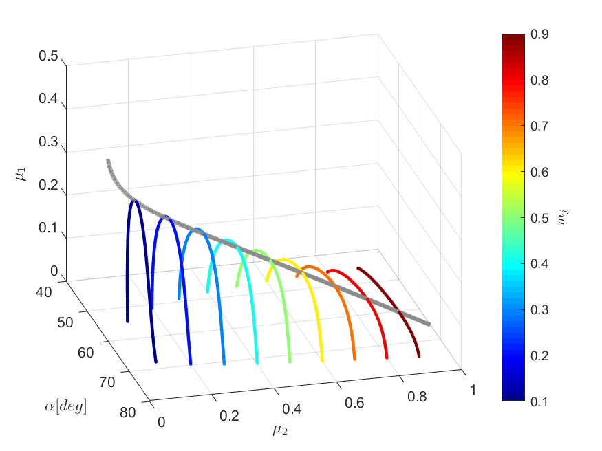
Figure 5: The $\mu_{1}(\mu_{2}=m_{j})$ curves for different values of $m_{j}$. The value of $m_{j}$ is indicated by the colour of the curve and it is measured on the colour-scale. The gray curve represents the peak values $M_{1}(\mu_{2})$.

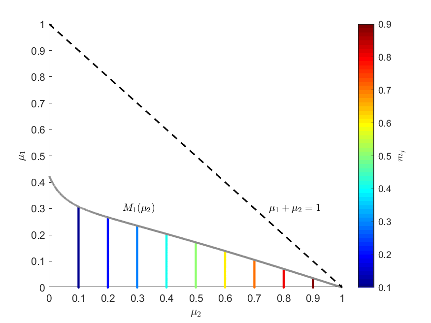
Figure 6: The curve $M_{1}(\mu_{2})$ on the plane $(\mu_{2},\mu_{1})$, coloured by gray. The coloured vertical lines correspond to the $\mu_{1}(\mu_{2}=m_{j})$ curves in Fig. 5. The value of $m_{j}$ is measured on the colour-scale.

On the $(\alpha,\mu_{1})$ plane, the intersections of the curves $\mu_{1}(\mu_{2}(\alpha,\beta)=c)$ and the horizontal lines $\mu_{1}=c$, where $0\leq c\leq 1$, give the solutions of Eqs. (6). The number of intersections can be assigned to each point of the $(\mu_{2},\mu_{1})$ plane. So examining the $(\mu_{2},\mu_{1})$ plane, for a given value of $\mu_{2}$, depending on the value of $\mu_{1}$, Eqs. (6) have:

• $0$ solution when $\mu_{1}>M_{1}(\mu_{2})$,

• $1$ solution when $\mu_{1}=M_{1}(\mu_{2})$,

• $2$ solutions when $\mu_{1}<M_{1}(\mu_{2})$.

For given parameters $m_{1}$ and $m_{2}$, all the possible concave type configurations are described by the combined solutions of both versions of Eqs. (6), that is when $\mu_{2}=m_{1}$ and $\mu_{2}=m_{2}$. Let $M_{m_{1}}$ and $M_{m_{2}}$ denote the functions $M_{1}(\mu_{2}=m_{1})$ and $M_{1}(\mu_{2}=m_{2})$, respectively. These functions are shown in Figs. 7 and 8 on the parameter plane $(m_{1},m_{2})$. Fig. 7, where $m_{1}$ and $m_{2}$ are measured on the horizontal and vertical axes, respectively, is actually a repetition of Fig. 6 with different notations. There are two solutions of Eqs. (6) for masses below the curve $M_{m_{1}}$ in Fig. 7, one solution on the curve $M_{m_{1}}$, and no (or zero) solution between the curve $M_{m_{1}}$ and the line $m_{1}+m_{2}=1$. Fig. 8, similarly to Fig. 7, where $m_{1}$ and $m_{2}$ are measured on the horizontal and vertical axes, respectively, is a mirrored version of Fig. 6 with respect to the diagonal $m_{1}=m_{2}$ with different notations. Thus the curve $M_{m_{2}}$ in Fig. 8 separates regions with no or two solutions (right or left from the curve $M_{m_{2}}$), while for mass values along the curve $M_{m_{2}}$ there is one solution. The number of solutions of Eqs. (6) is the sum of the solutions deduced from Figs. 7 and 8, except for the cases when $m_{1}=m_{2}$. Switching equal masses on the axis of symmetry does not lead to a new (affine class) solution, so summation, in this case, is omitted.

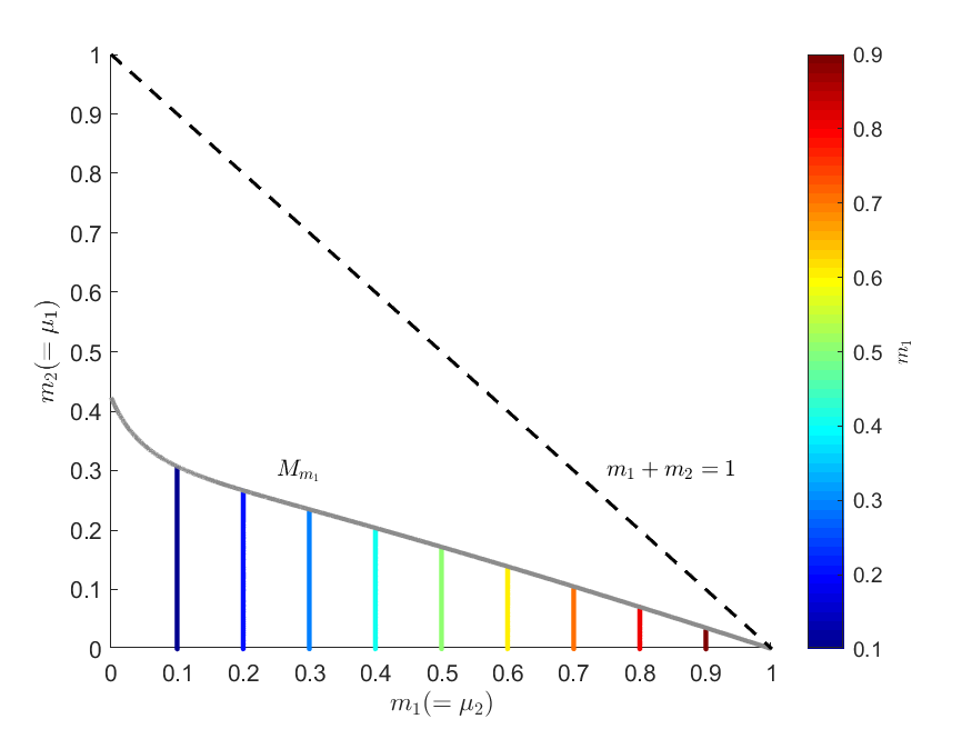
Figure 7: The $(m_{1},m_{2})$ parameter plane where the mass of the $\mu_{1}$-placed body (see Fig. 2) is measured on the $m_{2}$ axis. The mass of the $\mu_{2}$-placed body is represented on the $m_{1}$ axis. The $\mu_{1}(\mu_{2}=m_{1})$ curves from Fig. 5 are the coloured vertical lines. The gray curve illustrates the $M_{m_{1}}=M_{1}(\mu_{2}=m_{1})$ function.

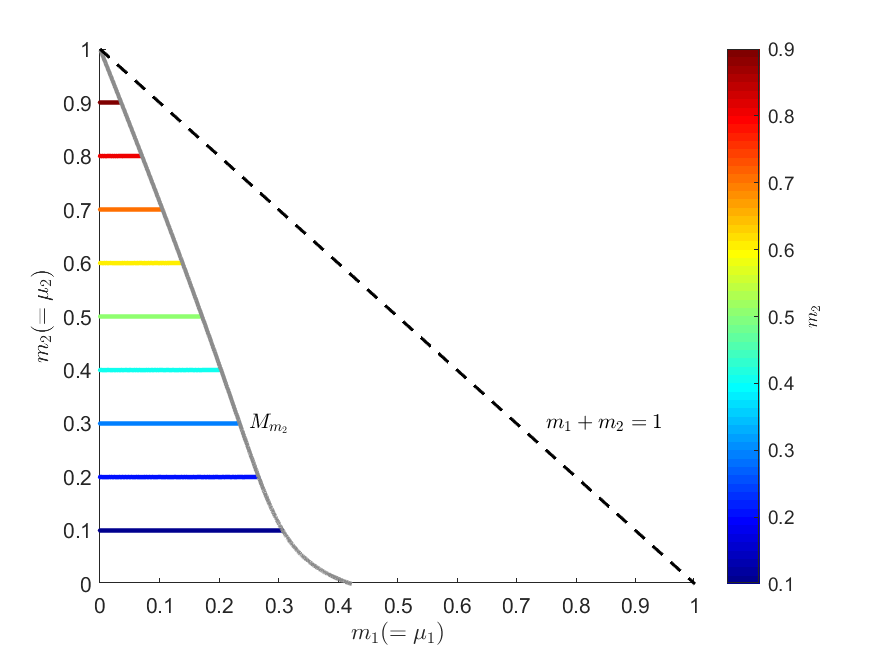
Figure 8: The $(m_{1},m_{2})$ parameter plane where the mass of the $\mu_{1}$-placed body (see Fig. 2) is measured on the $m_{1}$ axis. The mass of the $\mu_{2}$-placed body is represented on the $m_{2}$ axis. The $\mu_{1}(\mu_{2}=m_{2})$ curves from Fig. 5 are the coloured horizontal lines. The gray curve illustrates the $M_{m_{2}}=M_{1}(\mu_{2}=m_{2})$ function.

Fig. 9 is a combination of Figs. 7 and 8. The curves $M_{m_{1}}$, $M_{m_{2}}$ (both having orange and indigo parts in the figure) and the (green) line $m_{1}=m_{2}$ define different borders of various types, dividing the admissible mass parameter plane into distinct areas. The curves $M_{m_{1}}$ and $M_{m_{2}}$ intersect each other in the point $E(m_{1}\sim 0.25034,m_{2}\sim 0.25034)$ on the line $m_{1}=m_{2}$. To each pair of coordinates $(m_{1},m_{2})$ in Fig. 9 there corresponds a specific number of solutions of Eqs. (6). Table 1 summarizes these numbers.

Location of the point $(m_{1},m_{2})$	Nr. of solutions
inside region I.	0
on the orange curve and in point E	1
inside region II. and on the green section	2
on the indigo curve	3
inside region III.	4

Table 1: The number of concave deltoid type central configurations in the regions of Fig. 9.

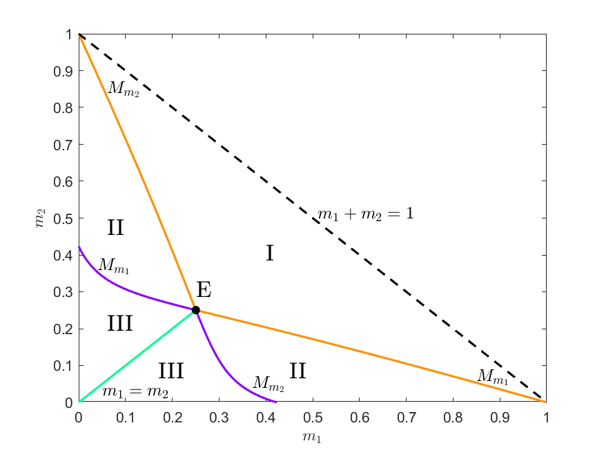
Figure 9: The three different types of subfields and their borders on the mass parameter plane.

As a summary of this subsection, we emphasize that the set of masses describing the configuration generally does not uniquely determine its shape. The number of isosceles trapezoidal and convex deltoid central configuration is 1. So, their masses uniquely determine the shape of the configuration. However, the number of concave deltoid configurations is between 0 and 4.

III An application: PSCCFB having Earth’s and Moon’s masses

As an application of the results of Sect. II, here we study the PSCCFB in such cases, where the bodies have Earth’s and Moon’s masses.

Let $m_{1}^{\prime}$, $m_{2}^{\prime}$, $m_{3}^{\prime}$ and $m_{4}^{\prime}$ denote the mass values of the four point-like bodies. Then let $m_{1}^{\prime}$ and $m_{2}^{\prime}$ be the mass of the Earth and Moon, respectively, that is $m_{1}^{\prime}=5.972\cdot 10^{24}$ kg and $m_{2}^{\prime}=7.349\cdot 10^{22}$ kg. We use the average lunar distance $384,400$ km as the unit of length. Depending on the values of $m_{3}^{\prime}$ and $m_{4}^{\prime}$, we study the following cases:

1. $m_{3}^{\prime}=m_{1}^{\prime}$ and $m_{4}^{\prime}=m_{2}^{\prime}$ (or $m_{3}^{\prime}=m_{2}^{\prime}$ and $m_{4}^{\prime}=m_{1}^{\prime}$),

2. $m_{3}^{\prime}=m_{4}^{\prime}>0$,

3. $m_{3}^{\prime}=m_{2}^{\prime}$ and $m_{4}^{\prime}>0$,

4. $m_{3}^{\prime}=m_{1}^{\prime}$ and $m_{4}^{\prime}>0$.

In the following subsections, we characterize the main features of each case.

III.1 Case A

In this case, the configuration takes an isosceles trapezoidal shape (see Fig. 2) and since $m_{2}^{\prime}<m_{1}^{\prime}$, thus $\mu=m_{2}^{\prime}/(m_{1}^{\prime}+m_{2}^{\prime})$. For the masses of the Earth and the Moon, $\mu=0.0122$. This type of configuration requires two pairs of bodies with equal masses. Thus $m_{3}^{\prime}=m_{1}^{\prime}$ and $m_{4}^{\prime}=m_{2}^{\prime}$ (or $m_{3}^{\prime}=m_{2}^{\prime}$ and $m_{4}^{\prime}=m_{1}^{\prime}$) regardless of the labelling of $m_{3}^{\prime}$ and $m_{4}^{\prime}$. The only constraint is that the bodies with mass $m_{1}^{\prime}$ and $m_{2}^{\prime}$ in that order have to be on the long and short bases of the trapezoid.

Eqs. (4) has a unique solution for any of its three parameters (giving one, the other two can be uniquely determined). For $\mu=0.0122$, it follows that $\alpha=66.7803^{\circ}$ and $\beta=54.1463^{\circ}$ (see Fig. 10).

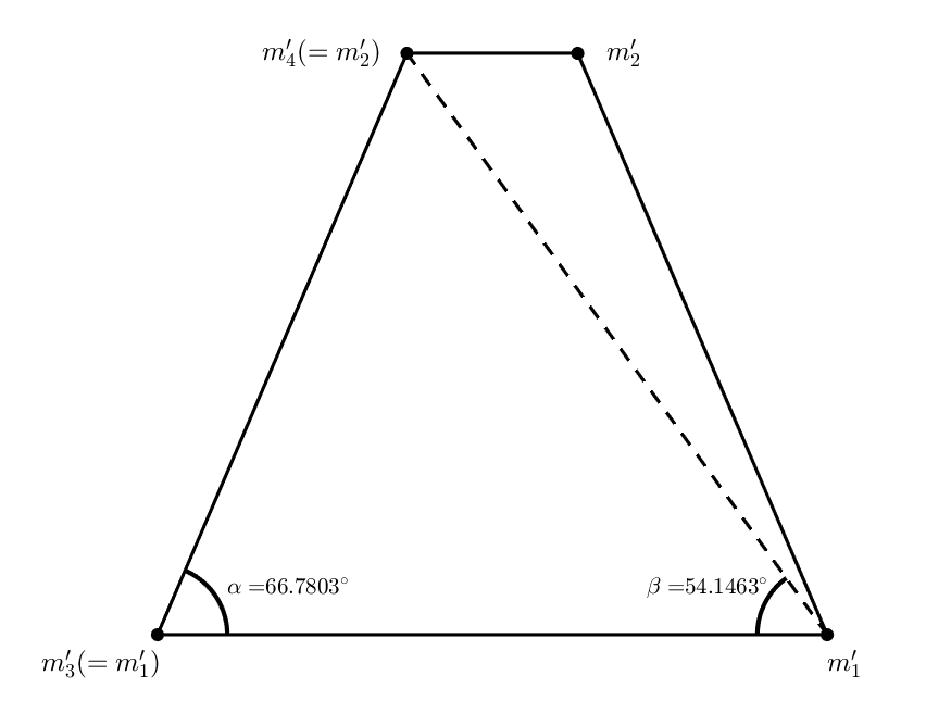
Figure 10: Isosceles trapezoidal shape central configuration with bodies that have masses of the Earth and Moon.

III.2 Case B

In this case, the deltoid-shaped configurations have the Earth’s and Moon’s mass bodies on the axis of symmetry (see Fig. 11). We calculated the non-dimensional and place-independent mass parameters as

$$m_{1}=\frac{m_{1}^{\prime}}{M},\quad m_{2}=\frac{m_{2}^{\prime}}{M},\quad m=\frac{m^{\prime}}{M},$$ (9)

where $M=m_{1}^{\prime}+m_{2}^{\prime}+2m^{\prime}$ is the unit of mass, and $m^{\prime}=m_{3}^{\prime}=m_{4}^{\prime}>0$, what we consider as an independent variable. We introduce the mass value $m^{\prime\prime}=m^{\prime}/m_{1}^{\prime}$ (the value of $m^{\prime}$ in Earth’s mass), to use it later as a reference in descriptions and illustrations.

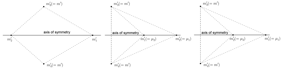
Figure 11: Deltoid-type configurations in Case B, where the bodies on the axis of symmetry have masses of the Earth and Moon.

We studied configurations where the value of $m^{\prime\prime}$ changes between negligible and Earth’s mass ($m^{\prime\prime}$ changes from 0 to 1). There is a unique convex configuration for any mass composition. We determined the number of the concave configurations with the help of Fig. 12, where we displayed the points $(m_{1},m_{2})$, calculated by using Eqs. (9), and coloured them according to the value of $m^{\prime\prime}$. The coloured curve crosses the curve $M_{m_{1}}$ when $m^{\prime\prime}=\nu_{1}=0.0111$, the curve $M_{m_{2}}$ when $m^{\prime\prime}=\nu_{2}=0.7114$. Table 2 lists the number of concave configurations (that changes between 0 and 4) depending on the value of $m^{\prime\prime}$.

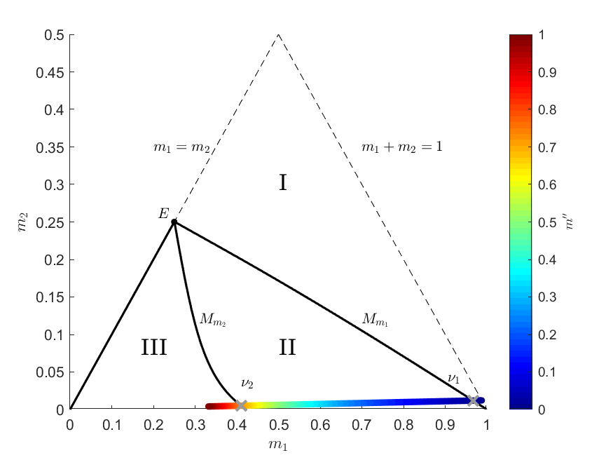
Figure 12: The coloured curve indicates the positions of the pairs $(m_{1},m_{2})$ for values of $m^{\prime\prime}$ between 0 and 1 Earth-mass according to the colour-scale. The figure corresponds to a part of Fig. 9. The number of the concave central configurations changes as the coloured curve goes through different regions, that is 0, 2, 4 in the regions I, II, III, respectively. There are 1 and 3 concave central configurations in the intersections with the $M_{m_{1}}$ and $M_{m_{2}}$ curves.

Condition	Number of configurations
$m^{\prime\prime}<\nu_{1}$	0
$m^{\prime\prime}=\nu_{1}$	1
$\nu_{1}<m^{\prime\prime}<\nu_{2}$	2
$m^{\prime\prime}=\nu_{2}$	3
$\nu_{2}<m^{\prime\prime}$	4

Table 2: The number of concave central configurations in Case B, depending on the value of $m^{\prime\prime}$.

We determined the locations of the equal-mass bodies $m_{3}^{\prime}$ and $m_{4}^{\prime}$ relative to the bodies $m_{1}^{\prime}$ and $m_{2}^{\prime}$ based on the value of $m^{\prime\prime}$, where the four bodies can form deltoid-type central configurations with the Earth-Moon axis being as the axis of symmetry. In Fig. 13, the curves $S_{i}$ and $S_{i}^{\prime}$ represent the locations of the equal-mass bodies $m^{\prime}3$ and $m^{\prime}4$, respectively. We calculated these curves by using Eqs. 5 and the formulae for the positions given in [3], and coloured them according to the value of $m^{\prime\prime}$. The points $P_{1}$ and $P_{1}^{\prime}$ mark the locations of the equal-mass bodies when $m^{\prime\prime}=\nu_{1}$ ($P_{1}$ stands for $m_{3}^{\prime}$, and $P_{1}^{\prime}$ for $m_{4}^{\prime}$), and $P_{2}$ (and $P_{2}^{\prime}$) when $m^{\prime\prime}=\nu_{2}$ (similarly $P_{2}$ for $m_{3}^{\prime}$ and $P_{2}^{\prime}$ for $m_{4}^{\prime}$). Note, that there are three $P_{2}$ (and $P_{2}$) points in accordance with Table 2. The curves $S_{3}$ and $S_{3}^{\prime}$ represent the locations of the equal-mass bodies that lead to convex configurations. Equal-mass bodies on the curves $S_{1}$ and $S_{1}^{\prime}$ or $S_{2}$ and $S_{2}^{\prime}$ result in a concave configuration. The curves $S_{1}$ and $S_{1}^{\prime}$ consist of two curves $S_{1a}$, $S_{1b}$ and $S_{1a}^{\prime}$, $S_{1b}^{\prime}$, respectively, that start from the points $P_{1}$ and $P_{1}^{\prime}$, respectively, when $m^{\prime\prime}=\nu_{1}$ and end when $m^{\prime\prime}=1$ as the value of $m^{\prime\prime}$ grows continuously. The curves $S_{1}$ and the point $P_{1}$ are located on the side of the Lagrangian point $L_{4}$ with respect to the Earth-Moon axis. Similarly, the curves $S_{2}$ and $S_{2}^{\prime}$ consist of two curves $S_{2a}$, $S_{2b}$ and $S_{2a}^{\prime}$, $S_{2b}^{\prime}$, respectively, that start from the points $P_{2}$ and $P_{2}^{\prime}$, respectively, when $m^{\prime\prime}=\nu_{2}$ and end when $m^{\prime\prime}=1$ as the value of $m^{\prime\prime}$ grows continuously. The curves $S_{2}$ are located on the side of the Lagrangian point $L_{5}$ with respect to the Earth-Moon axis. Table 3 summarizes the configuration parameters calculated at the endpoints of the curves $S_{i}$ and $S_{i}^{\prime}$.

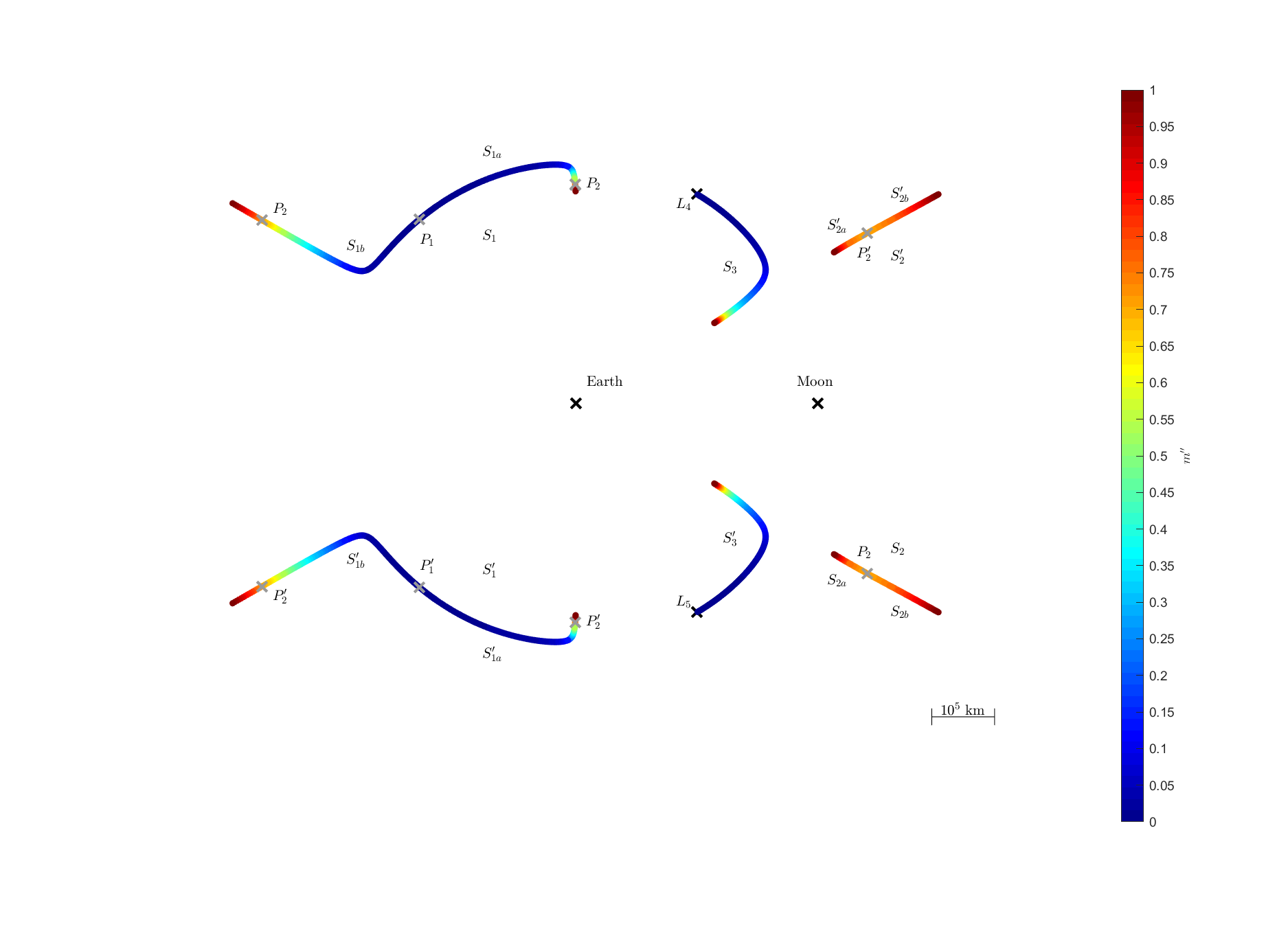
Figure 13: The coloured curves $S_{i}$ and $S_{i}^{\prime}$ represent the location of the equal-mass bodies in the Earth-Moon system in Case B. These are the places, where they can form planar, symmetric central configurations with the Earth and the Moon. The colour-scale is linear in Earth-mass.

Table 3: The configurations parameters calculated in Case B at the endpoints of the curves $S_{i}$ and $S_{i}^{\prime}$ in Figure 13.

Positions		Parameters
Curves	Points	$m^{\prime\prime}$	$\alpha$	$\beta$	$m_{1}$	$m_{2}$
$S_{1a}$ and $S_{1a}^{\prime}$	starting points $P_{1}$ and $P_{1}^{\prime}$	$\nu_{1}=0.0111$	$65.19^{\circ}$	$40.42^{\circ}$	$0.9667$	$0.0119$
	ending points	$1$	$48.79^{\circ}$	$0.18^{\circ}$	$0.3320$	$0.0041$
$S_{1b}$ and $S_{1b}^{\prime}$	starting points $P_{1}$ and $P_{1}^{\prime}$	$\nu_{1}=0.0111$	$65.19^{\circ}$	$40.42^{\circ}$	$0.9667$	$0.0119$
	ending points	$1$	$71.12^{\circ}$	$59.79^{\circ}$	$0.3320$	$0.0041$
$S_{2a}$ and $S_{2a}^{\prime}$	starting points $P_{2}$ and $P_{2}^{\prime}$	$\nu_{2}=0.7114$	$59.66^{\circ}$	$16.24^{\circ}$	$0.4107$	$0.0051$
	ending points	$1$	$59.62^{\circ}$	$6.14^{\circ}$	$0.3320$	$0.0041$
$S_{2b}$ and $S_{2b}^{\prime}$	starting points $P_{2}$ and $P_{2}^{\prime}$	$\nu_{2}=0.7114$	$59.66^{\circ}$	$16.24^{\circ}$	$0.4107$	$0.0051$
	ending points	$1$	$59.99^{\circ}$	$29.99^{\circ}$	$0.3320$	$0.0041$
$S_{3}$ and $S_{3}^{\prime}$	starting points	0	$30^{\circ}$	$30^{\circ}$	$0.9878$	$0.0122$
	ending points	$1$	$59.82^{\circ}$	$52.19^{\circ}$	$0.3320$	$0.0041$

To conclude, there is a convex deltoid configuration for any mass arrangement, while concave configuration are only possible if $m^{\prime\prime}\geq\nu_{1}$. Table 2 summarizes the number of concave-type configurations depending on the value of $m^{\prime\prime}$.

III.3 Case C

In this case, the deltoid-shaped configurations have two Moon-mass bodies separated by the axis of symmetry, which houses two bodies, one with an Earth- and one with an arbitrary mass (see Fig. 14). So we calculated the non-dimensional and place-independent masses as

$$m_{1}=\frac{m_{1}^{\prime}}{M},\quad m_{2}=\frac{m^{\prime}}{M},\quad m=\frac{m_{2}^{\prime}}{M},$$ (10)

where $M=m_{1}^{\prime}+2m_{2}^{\prime}+m^{\prime}$ is the unit of mass, $m_{2}^{\prime}=m_{3}^{\prime}$ and $m^{\prime}=m_{4}^{\prime}>0$ is an independent variable. Similarly to Case B, we introduce the mass value $m^{\prime\prime}=m^{\prime}/m_{1}^{\prime}$.

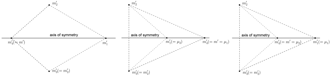
Figure 14: Deltoid-type configurations in Case C, where on the axis of symmetry, one body have the mass of the Earth, and the bodies that are separated by the axis of symmetry, have the mass of the Moon.

Similarly to Case B, we studied configurations for values of $m^{\prime\prime}$ between 0 and 1. There is a unique convex configuration for any mass composition. We deduced the number of concave configurations from Fig. 15, based on the descriptions in Fig. 9 and Table 1, where the points $(m_{1},m_{2})$, calculated by using Eqs. (10), are displayed and coloured according to the value of $m^{\prime\prime}$. The coloured curve crosses the curve $M_{m_{1}}$ when $m^{\prime\prime}=\nu=0.0137$. Table 4 lists the number of concave configurations (that changes between 0 and 2) depending on the value of $m^{\prime\prime}$.

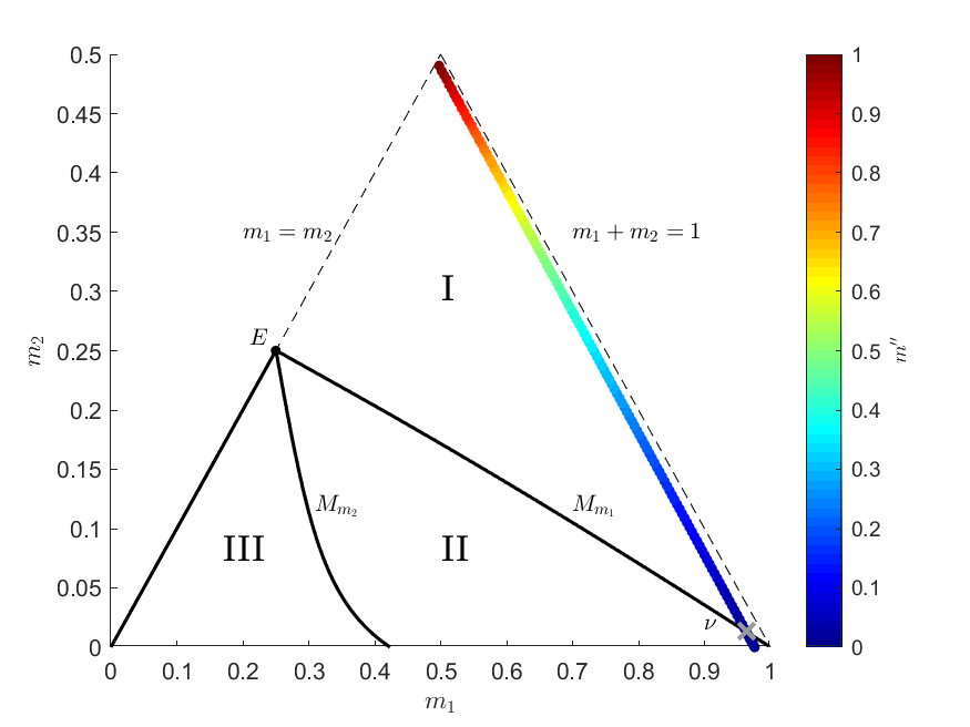
Figure 15: The coloured curve indicates the positions of the pairs $(m_{1},m_{2})$ for values of $m^{\prime\prime}$ between 0 and 1 Earth-mass according to the colour-scale. The figure corresponds to a part of Fig. 9. The number of the concave central configurations changes as the coloured curve goes through different regions, that is 2, 0 in the regions II, I, respectively. There is one concave central configurations in the intersection with the curve $M_{m_{1}}$.

Condition	Number of configurations
$m^{\prime\prime}<\nu$	2
$m^{\prime\prime}=\nu$	1
$m^{\prime\prime}>\nu$	0

Table 4: The number of concave central configurations in Case C, depending on the value of $m^{\prime\prime}$.

We calculated the locations of the bodies $m_{3}^{\prime}$ and $m_{4}^{\prime}$ relative to the bodies $m_{1}^{\prime}$ and $m_{2}^{\prime}$ based on the value of $m^{\prime\prime}$, where the four bodies can form a deltoid-type central configuration containing the Earth-Moon axis (see Fig. 14). In Figs. 16 and 17, the curves $M_{i}$ and $S_{i}$, coloured according to the value of $m^{\prime\prime}$, indicate the positions of the bodies $m_{3}^{\prime}$ and $m_{4}^{\prime}$, respectively, with respect to $m_{1}^{\prime}$ (Earth) and $m_{2}^{\prime}$ (Moon).

In Fig. 16, the curves $M_{1}$ and $S_{1}$ represent the locations of the bodies $m_{3}^{\prime}$ and $m_{4}^{\prime}$, respectively, leading to convex configurations. As the value of the $m^{\prime\prime}$ grows, the body $m_{4}^{\prime}$ heads toward the Lagrangian point $L_{4}$, while the body $m_{3}^{\prime}$ departing from it is getting farther away. The colours do not match in Figs. 15 and 16. Both colour-scales takes values between 0 and 1, but it is linear in Fig 15, and logarithmic in Fig. 16 for better visibility.

In Fig. 17, the curves $M_{i}$ and $S_{i}$ for $i=\{2,3\}$ represent the locations of the bodies $m_{3}^{\prime}$ and $m_{4}^{\prime}$, respectively, leading to concave configurations. The points $P_{m_{3}^{\prime}}$ and $P_{m_{4}^{\prime}}$ represent the position of the bodies $m_{3}^{\prime}$ and $m_{4}^{\prime}$, respectively, when $m^{\prime\prime}=\nu$. In Fig. 17, the curves $M_{i}$ start with $m^{\prime\prime}=0$ and converge toward the point $P_{m_{3}^{\prime}}$ as $m^{\prime\prime}$ grows toward $\nu$. Similarly, the curves $S_{i}$ begin at different points when $m^{\prime\prime}=0$ then head towards the point $P_{m_{4}^{\prime}}$ as $m^{\prime\prime}$ grows to $\nu$. The colours do not match in Figs. 15 and 17. Both colour-scales are linear, but their range is 0-1 in Fig. 15, and 0-0.001 in Fig. 17.

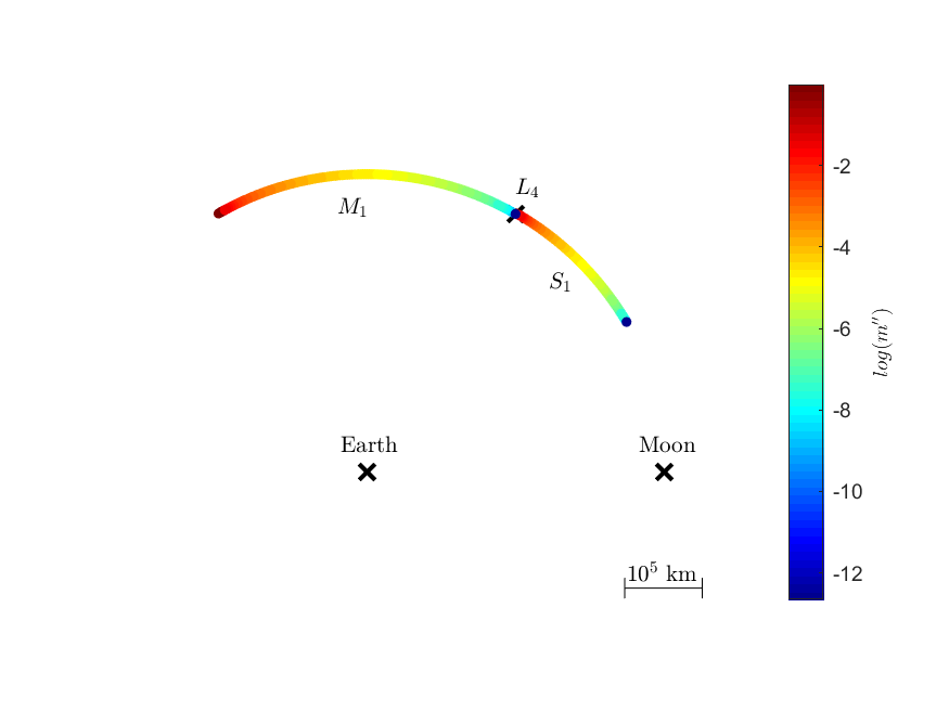
Figure 16: The coloured curves $M_{1}$ and $S_{1}$ represent the location of the bodies $m_{3}^{\prime}$ and $m_{4}^{\prime}$, respectively, to achieve convex configuration in Case C. The curves $M_{1}$ and $S_{1}$ are coloured according to the value of $m^{\prime\prime}$. The colour-scale is logarithmic in Earth-mass.

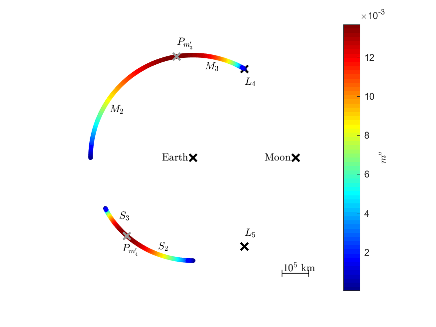
Figure 17: The coloured curves $M_{i}$ and $S_{i}$ for $i=\{2,3\}$ represent the location of the bodies $m_{3}^{\prime}$ and $m_{4}^{\prime}$, respectively, to achieve concave configuration in Case C when the Earth ($m_{1}^{\prime}$) is the inner body. The curves $M_{i}$ and $S_{i}$ are coloured according to the value of $m^{\prime\prime}$. The colour-scale is linear in Earth-mass.

Table 5: The configurations parameters calculated in Case C at the endpoints of the curves $S_{i}$ and $M_{i}$ in Figs. 16 and 17

Positions		Parameters
Curves	Points	$m^{\prime\prime}$	$\alpha$[deg]	$\beta$[deg]	$m_{1}$	$m_{2}$
$S_{1}$ and $M_{1}$	starting points	$0$	$59.99^{\circ}$	$15.77^{\circ}$	$0.9759$	$0.012$
	ending points	$1$	$30.11^{\circ}$	$30.11^{\circ}$	$0.4959$	$0.006$
$S_{2}$ and $M_{2}$	starting points	$0$	$45.05^{\circ}$	$0.01^{\circ}$	$0.9759$	$0.012$
	ending points $P_{m_{3}^{\prime}}$ and $P_{m_{4}^{\prime}}$	$\nu=0.0137$	$65.18^{\circ}$	$40.41^{\circ}$	$0.0132$	$0.9631$
$S_{3}$ and $M_{3}$	starting points	0	$74.9^{\circ}$	$59.99^{\circ}$	$0.976$	$0.012$
	ending points $P_{m_{3}^{\prime}}$ and $P_{m_{4}^{\prime}}$	$\nu=0.0137$	$65.18^{\circ}$	$40.41^{\circ}$	$0.0132$	$0.9631$

To conclude, there is one convex deltoid-type configuration for any value of $m^{\prime\prime}$, while concave configurations are only possible if $m^{\prime\prime}\leq\nu$. Table 4 summarizes the number of concave-type configurations based on the value of $m^{\prime\prime}$. Table 5 lists the configuration parameters calculated at the endpoints of the curves $M_{i}$ and $S_{i}$.

III.4 Case D

In this case, the deltoid-shaped configurations have two Earth-mass bodies separated by the axis of symmetry, which contains two bodies, one with a Moon- and one with an arbitrary mass (see Fig. 18). So we calculated the non-dimensional and place-independent masses as

$$m_{1}=\frac{m^{\prime}}{M},\quad m_{2}=\frac{m_{2}^{\prime}}{M},\quad m=\frac{m_{1}^{\prime}}{M}.$$ (11)

where $M=2m_{1}^{\prime}+m_{2}^{\prime}+m^{\prime}$ is the unit of mass, $m_{1}^{\prime}=m_{3}^{\prime}$ and $m^{\prime}=m_{4}^{\prime}>0$ is an independent variable. Similarly to Cases B and C, we introduce the mass value $m^{\prime\prime}=m^{\prime}/m_{1}^{\prime}$.

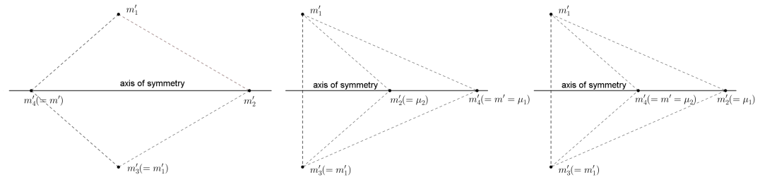
Figure 18: Deltoid-type configurations in Case D, where on the axis of symmetry, one body have the mass of the Moon, and the bodies that are separated by the axis of symmetry, have the mass of the Earth.

Similarly to Cases B and C, we studied configurations for values of $m^{\prime\prime}$ between 0 and 1. There is one convex configuration for all values of $m^{\prime\prime}$. To determine the number of concave configurations, we calculated the curve $(m_{1},m_{2})$, by using Eqs. (11), and coloured it according to the value of $m^{\prime\prime}$ (see Fig. 19). Then we deduced the number of the concave configurations using the descriptions in Fig. 9 and Table 1. In Fig. 19, the coloured curve is inside the two regions of III, crossing the line $m_{1}=m_{2}$ at $m^{\prime\prime}=\nu=0.0123$. So there are two different concave configurations when $m^{\prime\prime}=\nu$. For any other value of $m^{\prime\prime}$, there are four concave configurations.

Figure 19: The coloured curve indicates the positions of the pairs $(m_{1},m_{2})$ for values of $m^{\prime\prime}$ between 0 and 1 Earth-mass according to the colour-scale. The number of the concave central configurations is four, since the coloured curve is inside the region III. Except, when it intersects the line $m_{1}=m_{2}$ at $m^{\prime\prime}=0.0123$, then the number is two.

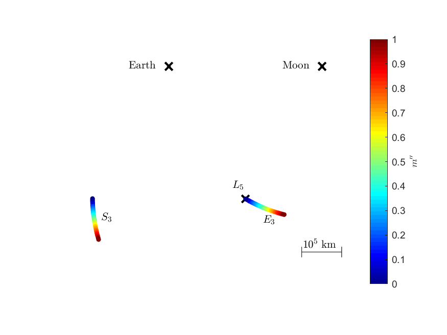
Figure 20: The coloured curves $E_{3}$ and $S_{3}$ represent the location of the bodies $m_{3}^{\prime}$ and $m_{4}^{\prime}$, respectively, to achieve convex configuration in Case D. The curves $E_{3}$ and $S_{3}$ are coloured according to the value of $m^{\prime\prime}$. The colour-scale is linear in Earth-mass.

Similarly to Cases B and C, we calculated the locations of the bodies $m_{3}^{\prime}$ and $m_{4}^{\prime}$ relative to the bodies $m_{1}^{\prime}$ and $m_{2}^{\prime}$ based on the value of $m^{\prime\prime}$, where the four bodies can form a deltoid-type central configuration containing the Earth-Moon axis (see Fig. 18). The role of the In Figs. 20, 21 and 22 the curves $E_{i}$ and $S_{i}$, coloured according to the value of $m^{\prime\prime}$, denote the locations of the bodies $m_{3}^{\prime}$ and $m_{4}^{\prime}$, respectively.

In Fig. 20, the curves $E_{3}$ and $S_{3}$ represent the locations of the bodies $m_{3}^{\prime}$ and $m_{4}^{\prime}$, respectively, that together with the Earth ($m_{1}^{\prime}$) and Moon ($m_{2}^{\prime}$) form a convex central configuration. The curves $E_{i}$ and $S_{i}$ for $i=\{1,2\}$ represent the locations of the bodies $m_{3}^{\prime}$ and $m_{4}^{\prime}$, respectively, leading to concave configurations when the inner body of the configuration is the Moon ($m_{2}^{\prime}$) (see Fig. 21), and for $i=\{4,5\}$ when the inner body is the body $m_{4}^{\prime}$ (see Fig. 22). The masses $m_{1}$ and $m_{2}$ defined by Eqs. (11) are the same at the endpoints of the curves $E_{i}$ and $S_{i}$. When $m^{\prime\prime}=0$, then $m_{1}=0$ and $m_{2}=0.0061$, and when $m^{\prime\prime}=1$, then $m_{1}=0.3320$ and $m_{2}=0.0041$. Table 6 contains the angles $\alpha$ and $\beta$ calculated at the endpoints of the curves $E_{i}$ and $S_{i}$.

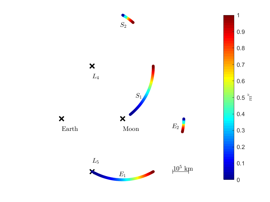
Figure 21: The coloured curves $E_{i}$ and $S_{i}$ for $i=\{1,2\}$ represent the location of the bodies $m_{3}^{\prime}$ and $m_{4}^{\prime}$, respectively, to achieve concave configuration in Case D when the inner body is the Moon ($m_{2}^{\prime}$). The curves $E_{i}$ and $S_{i}$ are coloured according to the value of $m^{\prime\prime}$. The colour-scale is linear in Earth-mass.

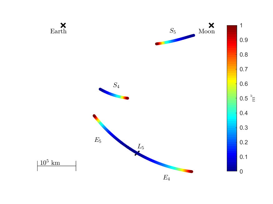
Figure 22: The coloured curves $E_{i}$ and $S_{i}$ for $i=\{4,5\}$ represent the location of the bodies $m_{3}^{\prime}$ and $m_{4}^{\prime}$, respectively, to achieve concave configuration in Case D when the inner body is the body $m_{4}^{\prime}$. The curves $E_{i}$ and $S_{i}$ are coloured according to the value of $m^{\prime\prime}$. The colour-scale is linear in Earth-mass.

Table 6: The configuration angle parameters $\alpha$ and $\beta$ calculated in Case D at the endpoints of the curves $E_{i}$ and $S_{i}$.

Positions		Parameters
Curves	Points	$\alpha$[deg]	$\beta$[deg]
$S_{1}$ and $E_{1}$	starting points	$63.63^{\circ}$	$59.99^{\circ}$
	ending points	$59.99^{\circ}$	$29.99^{\circ}$
$S_{2}$ and $E_{2}$	starting points	$59.57^{\circ}$	$0.01^{\circ}$
	ending points	$59.63^{\circ}$	$6.14^{\circ}$
$S_{3}$ and $E_{3}$	starting points	$59.99^{\circ}$	$59.89^{\circ}$
	ending points	$59.82^{\circ}$	$52.82^{\circ}$
$S_{4}$ and $E_{4}$	starting points	$60^{\circ}$	$0.05^{\circ}$
	ending points	$48.79^{\circ}$	$0.18^{\circ}$
$S_{5}$ and $E_{5}$	starting points	$60^{\circ}$	$55.55^{\circ}$
	ending points	$71.12^{\circ}$	$59.79^{\circ}$

To conclude, there is one convex deltoid-type configuration for any value of $m^{\prime\prime}$. The number of concave configurations is two when $m^{\prime\prime}=0.0123$, and four for other values of $m^{\prime\prime}$.

IV Summary

In this paper we studied the planar symmetric central configurations of four bodies.

In Sect. II.1, we overviewed our angle-based models for the PSCCFB, which provide an easy formalism for the computation of the masses, based on the shape of the configurations representing the solutions of the inverse problem (see Refs.[3] and [2]). In Sect. II.2 we overviewed our shape-type counting method for the PSCCFB, which applies when the disposition of the masses within the configuration is known (see Ref. [2]). We studied the cases when the location of the masses is arbitrary, representing the solution of the direct problem. There is a unique isosceles trapezoid and convex deltoid-shaped central configuration as presented in [2]. The number of the concave deltoid-shaped central configurations with different shapes is between 0 and 4. It depends on the set of masses of the configuration. We presented a diagram-based method to determine this number based on the masses.

In Sect. III applying the tools presented in Sect. II, we examined PSCCFB containing at least one pair of bodies having masses of the Earth and Moon. We identified four different possible cases. The number of central configurations with different shapes in Case A is 1, in Case B is between 1 and 5, in Case C is between 1 and 3, in Case D is 3 or 5.

Appendix A The $a_{0}$, $a_{1}$, $b_{0}$, $b_{1}$ coefficients

Convex case:

$$a_{0} =\tan\alpha\left(\cos^{3}\alpha-\frac{1}{8}\right),$$

$$b_{0} =\tan\beta\left(\cos^{3}\beta-\frac{1}{8}\right),$$

$$a_{1} =\frac{1}{(\tan\alpha+\tan\beta)^{2}}+\tan\beta\left(\frac{1}{8}-\cos^{3}\alpha-\cos^{3}\beta\right)-\frac{\tan\alpha}{8},$$

$$b_{1} =\frac{1}{(\tan\alpha+\tan\beta)^{2}}+\tan\alpha\left(\frac{1}{8}-\cos^{3}\alpha-\cos^{3}\beta\right)-\frac{\tan\beta}{8},$$

Concave case:

$$a_{0} =\tan\alpha\left(\cos^{3}\alpha-\frac{1}{8}\right),$$

$$b_{0} =-\tan\beta\left(\cos^{3}\beta-\frac{1}{8}\right),$$

$$a_{1} =\frac{1}{(\tan\alpha-\tan\beta)^{2}}+\tan\beta\left(\frac{1}{8}-\cos^{3}\alpha-\cos^{3}\beta\right)-\frac{\tan\alpha}{8},$$

$$b_{1} =\frac{1}{(\tan\alpha-\tan\beta)^{2}}+\tan\alpha\left(\frac{1}{8}-\cos^{3}\alpha-\cos^{3}\beta\right)+\frac{\tan\beta}{8},$$

Note that there are misprints in the coefficients $a_{1}$ and $b_{1}$ in the appendix of the paper [2].

References

- [1] Albouy A., Cabral H. E., and Santos A. A. (2012). Some problems on the classical n-body problem. Celestial Mechanics and Dynamical Astronomy, 113(4):369–375.
- [2] Czirják Z. and Érdi B. (2019). A study on the planar symmetric central configurations of four bodies using angles. Romanian Astronomical Journal, 29(1):59–74.
- [3] Érdi B. and Czirják Z. (2016). Central configurations of four bodies with an axis of symmetry. Celestial Mechanics and Dynamical Astronomy, 125(1):33–70.
- [4] Euler L. (1767). De motu rectilineo trium corporum se mutuo attrahentium. Novi commentarii academiae scientiarum Petropolitanae, 11:144–151.
- [5] Lagrange J.L. (1772). Essai sur le probleme des trois corps. Prix de l’académie royale des Sciences de paris, 9:292.
- [6] Laplace P. S. (1789). Sur quelques points du systeme du monde. Mémoires de l’Académie royale des Sciences de Paris, page 553.
- [7] Saari D. G. (2011). Central configuration - A problem for the twenty-first century. Exped. Math. MAA Spectrum, pages 283–295.
- [8] Smale S. (1970). Topology and mechanics. II. Inventiones mathematicae, 11(1): 45–64.
- [9] Smale S. (1998). Mathematical problems for the next century. The mathematical intelligencer, 20(2):7–15.