Dark Matter and $(g-2)_{\mu,e}$ in radiative Dirac neutrino mass models

Abstract

The origin of neutrino mass is a mystery, so is its nature, namely, whether neutrinos are Dirac or Majorana particles. On top of that, hints of large deviations of the muon and the electron anomalous magnetic moments (AMMs) are strong evidence for physics beyond the Standard Model. In this work, piecing these puzzles together, we propose a class of radiative Dirac neutrino mass models to reconcile $(g-2)_{\mu,e}$ anomalies with neutrino oscillation data. In this framework, a common set of new physics (NP) states run through the loops that generate non-zero neutrino mass and, due to chiral enhancement, provide substantial NP contributions to lepton AMMs. In addition, one of the three models studied in this work offers a Dark Matter candidate automatically stabilized by the residual symmetry, whose phenomenology is non-trivially connected to the other two puzzles mentioned above. Finally, our detailed numerical analysis reveals a successful resolution to these mysteries while being consistent with all colliders and cosmological constraints.

I Introduction

The Standard Model (SM) of particle physics is the most successful theory in particle physics that describes the fundamental interactions between elementary particles. Despite its major triumph, it is not perfect- it cannot explain the origin of neutrino mass or dark matter (DM). Moreover, the SM is under scrutiny since its predicted values of the muon and the electron anomalous magnetic moments (AMMs) are in tension with experimental measurements. There is a longstanding discrepancy in the muon AMM measured at BNL in 2006 Bennett:2006fi . A new measurement performed at the Fermilab Abi:2021gix in 2021 is in excellent agreement with BNL’s result, and combinedly they correspond to a large $4.2\sigma$ disagreement with the SM prediction Aoyama:2020ynm (for original works, see Refs. Aoyama:2012wk ; Aoyama:2019ryr ; Czarnecki:2002nt ; Gnendiger:2013pva ; Davier:2017zfy ; Keshavarzi:2018mgv ; Colangelo:2018mtw ; Hoferichter:2019mqg ; Davier:2019can ; Keshavarzi:2019abf ; Kurz:2014wya ; Melnikov:2003xd ; Masjuan:2017tvw ; Colangelo:2017fiz ; Hoferichter:2018kwz ; Gerardin:2019vio ; Bijnens:2019ghy ; Colangelo:2019uex ; Blum:2019ugy ; Colangelo:2014qya ):

$$\Delta a_{\mu}=(2.51\pm 0.59)\times 10^{-9}.$$ (1)

On the other hand, precise measurement of the fine-structure constant using Cesium atom at the Berkeley National Laboratory Parker:2018vye in 2018 yields,

$$\alpha^{-1}(C_{s})=137.035999046(27).$$ (2)

This result corresponds to a negative $2.4\sigma$ deviation of the electron AMM with respect to the SM value Aoyama:2017uqe :

$$\Delta a_{e}=(-8.8\pm 3.6)\times 10^{-13}.$$ (3)

These discrepancies are large in magnitude, and the opposite sign between them is somewhat puzzling and hints towards physics beyond the SM (BSM). For attempts to solve these discrepancies simultaneously in BSM frameworks, see, e.g., Refs. Giudice:2012ms ; Davoudiasl:2018fbb ; Crivellin:2018qmi ; Liu:2018xkx ; Dutta:2018fge ; Han:2018znu ; Crivellin:2019mvj ; Endo:2019bcj ; Abdullah:2019ofw ; Bauer:2019gfk ; Badziak:2019gaf ; Hiller:2019mou ; CarcamoHernandez:2019ydc ; Cornella:2019uxs ; Endo:2020mev ; CarcamoHernandez:2020pxw ; Haba:2020gkr ; Bigaran:2020jil ; Jana:2020pxx ; Calibbi:2020emz ; Chen:2020jvl ; Yang:2020bmh ; Hati:2020fzp ; Dutta:2020scq ; Botella:2020xzf ; Chen:2020tfr ; Dorsner:2020aaz ; Arbelaez:2020rbq ; Jana:2020joi ; Chua:2020dya ; Chun:2020uzw ; Li:2020dbg ; DelleRose:2020oaa ; Kowalska:2020zve ; Hernandez:2021tii ; Bodas:2021fsy ; Cao:2021lmj ; Mondal:2021vou ; CarcamoHernandez:2021iat ; Han:2021gfu ; Escribano:2021css ; CarcamoHernandez:2021qhf ; Chang:2021axw ; Chowdhury:2021tnm ; Bharadwaj:2021tgp ; Borah:2021khc ; Bigaran:2021kmn ; PadmanabhanKovilakam:2022FN ; Li:2021wzv ; Biswas:2021dan ; Julio:2022ton ; Julio:2022bue .

The observation of neutrino oscillations Super-Kamiokande:1998kpq ; Super-Kamiokande:2001ljr ; SNO:2002tuh ; KamLAND:2002uet ; KamLAND:2004mhv ; K2K:2002icj ; MINOS:2006foh was the first conclusive evidence that the SM is incomplete and must be extended. Although the existence of non-zero neutrino masses has been firmly established, the nature of neutrinos, viz. Dirac or Majorana is still unknown. As widely known, observation of neutrinoless double beta decay (see, e.g., Ref. Dolinski:2019nrj ) would settle this issue and establish the Majorana nature of neutrinos; however, all experiments so far have null results. Similarly, despite the discovery that about eighty percent of the Universe’s gravitating matter is non-luminous, we are yet to know anything about the nature of DM (see, e.g., Young:2016ala ).

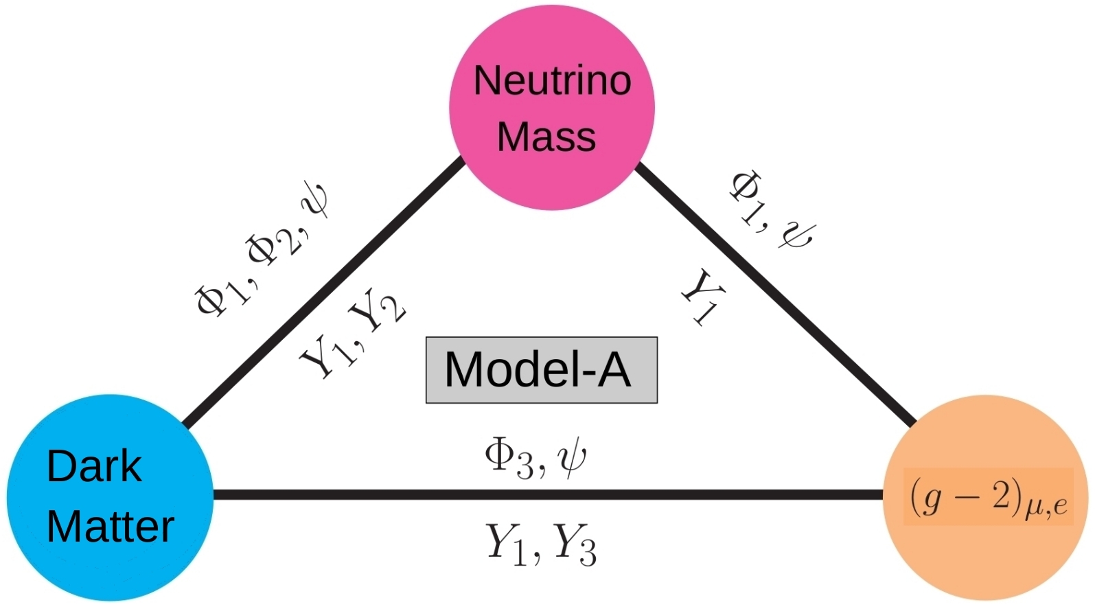
Figure 1: Schematic diagram demonstrating the link between neutrino mass generation, lepton $g-2$ anomalies, and Dark Matter in one of the benchmark models (Model-A) proposed in this work. See text for details.

This work considers neutrinos as Dirac particles, and non-zero neutrino masses originate from quantum corrections. This framework proposes a simultaneous solution to the muon and the electron AMMs that is non-trivially linked to the neutrino mass generation mechanism. New physics (NP) contributions to the lepton $g-2$ and non-zero neutrino masses arise via one-loop corrections mediated by a common set of BSM particles. We present a class of radiative Dirac neutrino mass models that share these same features and study in detail a particular model (dubbed as Model-A) belonging to this class that also addresses the DM puzzle and offers rich collider phenomenology. Remarkably, the stability of the DM is guaranteed by the residual symmetry that emerges after $U(1)_{B-L}$ gauge symmetry is spontaneously broken. In Model-A, all these puzzles are deeply intertwined, which is illustrated in Fig. 1.

The paper is organized as follows: in Sec. II, we discuss the general framework, and in Sec. III, we provide details of the set of models under investigation. Next, we discuss the experimental constraints in Sec. IV and carry out a detailed DM phenomenology for Model-A in Sec. V. Finally, we conclude in Sec. VI.

II Setup

Neutrinos being Dirac in nature requires the presence of right-handed partners $\nu_{R_{i}}$ ($i=1-3$), which automatically allows for tree-level neutrino mass via the term $-\mathcal{L}_{y}\supset Y_{\nu}\overline{L}\epsilon H^{\ast}\nu_{R}$ when the SM Higgs, $H$ acquires a vacuum expectation value (VEV); here $L$ is the SM lepton doublet, and $\epsilon$ is the Levi-Civita tensor. This, however, demands $y_{\nu}\sim\mathcal{O}(10^{-11})$ to be consistent with experimental data, which is seemingly unnatural tHooft:1979rat since the Yukawa couplings of the charged fermions in the SM are typically in the range $10^{-6}-1$. On the contrary, it is aesthetically attractive to generate Dirac neutrino mass radiatively that would naturally require the corresponding Yukawa couplings typically in the range $10^{-3}-1$. Symmetry arguments can naturally forbid the aforementioned tree-level term to achieve this. In this work, we accomplish this by extending the SM gauge symmetry by $U(1)_{B-L}$ Davidson:1978pm ; Mohapatra:1980qe ; in the literature, various types of symmetries are imposed to realize radiative Dirac mass, see, e.g., Refs. Mohapatra:1987hh ; Mohapatra:1987nx ; Balakrishna:1988bn ; Branco:1978bz ; Babu:1988yq ; Gu:2007ug ; Farzan:2012sa ; Okada:2014vla ; Ma:2016mwh ; Bonilla:2016diq ; Wang:2016lve ; Ma:2017kgb ; Yao:2017vtm ; Wang:2017mcy ; Helo:2018bgb ; Reig:2018mdk ; Han:2018zcn ; Kang:2018lyy ; Yao:2018ekp ; Calle:2018ovc ; CentellesChulia:2018gwr ; Bonilla:2018ynb ; Calle:2018ovc ; Carvajal:2018ohk ; CentellesChulia:2018bkz ; Ma:2019yfo ; Bolton:2019bou ; Saad:2019bqf ; Bonilla:2019hfb ; Dasgupta:2019rmf ; CentellesChulia:2019gic ; CentellesChulia:2019xky ; Jana:2019mez ; Enomoto:2019mzl ; Ma:2019byo ; Restrepo:2019soi ; Jana:2019mgj ; Nanda:2019nqy ; Wang:2020dbp ; Borgohain:2020csn ; Mahanta:2021plx ; Bernal:2021ezl ; Biswas:2021kio ; Calle:2021tez ; De:2021crr ; Bernal:2021ppq ; Mishra:2021ilq .

Gauge anomaly cancellation conditions then require the right-handed neutrinos to carry charges which are either $\nu_{R_{1,2,3}}=\{-1,-1,-1\}$ or $\nu_{R_{1,2,3}}=\{5,-4,-4\}$ Montero:2007cd ; Machado:2010ui ; Machado:2013oza . We choose the latter charge assignment since the former allows the unwanted tree-level term in the Lagrangian. To spontaneously break $U(1)_{B-L}$, we employ a SM singlet scalar that carries three units of $B-L$ charge: $\sigma\sim(1,1,0,3)$. Then non-zero mass for the neutrinos appears through loop diagrams when both the electroweak (EW) and $U(1)_{B-L}$ symmetries are broken (in our setup, the only two fields that acquire VEVs are $H$ and $\sigma$). These loop diagrams originate from ultra-violate (UV) completion of the following unique dimension five operator:

$$-\mathcal{L}_{d=5}=\frac{y_{ij}}{\Lambda}\;\overline{L}_{i}\epsilon H^{\ast}{\nu_{R}}_{j}\sigma+h.c.,$$ (4)

where $i=1-3$ and $j=2,3$. In the following, we very briefly summarize how to construct UV-complete one-loop models utilizing this $d=5$ operator; for details, we refer the reader directly to Ref. Jana:2019mgj (we adopt the nomenclature used therein).

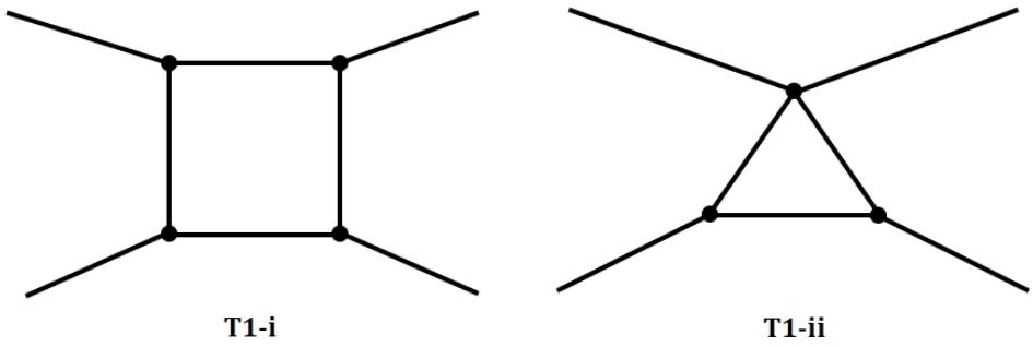
Figure 2: Two distinct one-loop topologies that lead to Dirac neutrino mass. See text for details.

One-loop Dirac neutrino mass models can be constructed out of two independent topologies: T1-i and T1-ii that are shown in Fig. 2. Depending on the Lorentz structures (i.e, fermion-fermion-scalar or scalar-scalar-scalar interaction) associated with these vertices, three different diagrams (T1-i-1, T1-i-2, and T1-i-3) can be drawn for topology T1-i. On the other hand, for T1-ii, there is a unique diagram labeled as T1-ii-1. Moreover, by interchanging the external scalar legs of some of these diagrams, in total, eight minimal models can be fabricated Jana:2019mgj .

In this work, we focus on the diagram T1-ii-1 and propose explicit models in light of the muon and the electron $g-2$. In particular, we formulate three minimal models (labeled as Model-A, Model-B, Model-C), each of which, in addition to correctly reproducing neutrino oscillation data, addresses both $(g-2)_{\mu,e}$. Among these three models, DM can also be incorporated within Model-A. Moreover, this model shows profound correlations among the neutrino mass, DM, and $(g-2)_{\mu,e}$ as well as offers rich collider phenomenology. Stunningly, no ad hoc symmetry needs to be imposed by hand to realize this dark matter; instead, its stability is assured by a leftover discrete symmetry resulting from the breaking of $U(1)_{B-L}$ gauge symmetry.

Since topology T1-i in Fig. 2 has a 4-particle vertex, there is a unique choice of attaching external $H$ and $\sigma$ lines to it to form the $d=5$ operator of Eq. (4). Completion of the neutrino mass diagram then requires (i) a vector-like Dirac fermion $\psi$ (of three generations) and (ii) two distinct BSM scalars $\Phi_{1,2}$; see the top diagram in Fig. 3. With only these new states, corrections to muon and electron AMMs are too small to be consistent with experimental findings. However, large NP contributions to lepton $g-2$ can naturally arise within this setup via chirally enhanced terms that are proportional to vector-like fermion mass by introducing (iii) the third scalar $\Phi_{3}$; see the bottom diagram in Fig. 3.

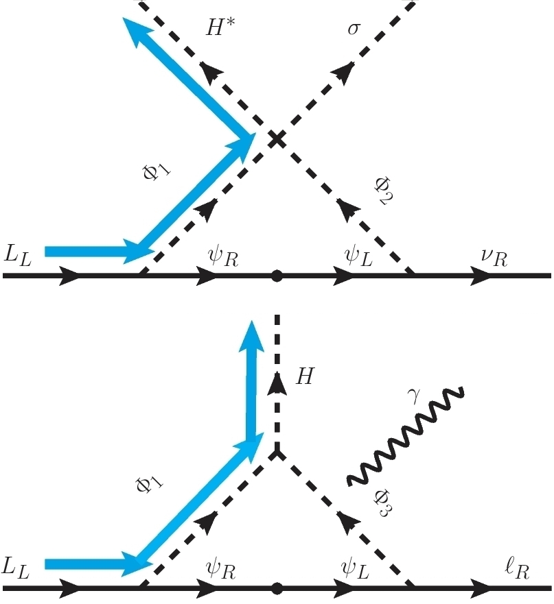
Figure 3: In this class of models, neutrino mass (lepton $g-2$) originates from the diagram on the top (bottom). The blue line shows the direction of the iso-doublet flow in an economical fashion. Any other direction of this flow would correspond to non-minimal model, see text for details.

In Fig. 3, blue lines correspond to the iso-doublet flow drawn to indicate the most economical way to build this class of models. As shown in Fig. 3, this choice requires a single BSM scalar field to be iso-doublet (and no BSM iso-doublet fermion is required). This way, the least number of new degrees of freedom is introduced in a given model belonging to this class (this is our minimality criterion). Minimal models of this class then contain four BSM fields that propagate inside the loops and contribute to neutrino mass as well as lepton $g-2$, and have the following quantum numbers:

$$\psi\sim(1,1,Y,\beta),$$ (5)

$$\Phi_{1}\sim(1,2,-Y-\frac{1}{2},-\beta-1),$$ (6)

$$\Phi_{2}\sim(1,1,Y,\beta+4),$$ (7)

$$\Phi_{3}\sim(1,1,Y+1,\beta+1),$$ (8)

where, $Y$ and $\beta$ are the hypercharge and the $B-L$ charge, respectively, carried by the vector-like fermion. It is important to note that: (a) if $Y=-1$ then $\beta=2$ is not allowed. In this case, a cubic term of the form $\mathcal{V}\supset H^{\dagger}\Phi_{1}\sigma$ is allowed, which would lead to an induced VEV for $\Phi_{1}$ resulting in a tree-level Dirac mass for the neutrinos via $\mathcal{L}_{y}\supset\overline{L}\epsilon\Phi_{1}^{\ast}\nu_{R}$. Furthermore, (b) if $Y=0$ then $\beta=-1$ is not allowed. In this scenario, a combination of three terms $\mathcal{L}_{y}\supset\overline{L}\epsilon H^{\ast}\psi_{R}$, $\overline{\psi}_{L}\sigma\nu_{R}$, and $m_{\psi}\overline{\psi}_{L}\psi_{R}$ in the Lagrangian would generate neutrino mass via tree-level Dirac seesaw (once VEVs of $H$ and $\sigma$ are inserted).

III Models

This section discusses three different versions of models belonging to the class introduced in the previous section. For simplicity, we restrict ourselves to the case of $|Y|\leq 1$. We label these models as Model-A ($Y=0$), Model-B ($Y=-1$), and Model-C ($Y=+1$) for which the full quantum numbers of NP states are specified in Table 1. In the following text, we provide all the necessary details of these models.

Fields	Model-A ($Y=0,\beta\neq-1$)	Model-B ($Y=-1,\beta\neq 2$)	Model-C ($Y=+1$)
$\psi$	$\psi^{0}(1,1,0,\beta)$	$\psi^{-}(1,1,-1,\beta)$	$\psi^{+}(1,1,+1,\beta)$
$\Phi_{1}$	$\phi=\begin{pmatrix}\phi^{0}\\ \phi^{-}\end{pmatrix}=(1,2,-\frac{1}{2},-\beta-1)$	$\phi=\begin{pmatrix}\phi^{+}\\ \phi^{0}\end{pmatrix}=(1,2,+\frac{1}{2},-\beta-1)$	$\phi=\begin{pmatrix}\phi^{-}\\ \phi^{--}\end{pmatrix}=(1,2,-\frac{3}{2},\beta-1)$
$\Phi_{2}$	$S^{0}(1,1,0,\beta+4)$	$\eta^{-}(1,1,-1,\beta+4)$	$\eta^{+}(1,1,+1,\beta+4)$
$\Phi_{3}$	$\eta^{+}(1,1,+1,\beta+1)$	$S^{0}(1,1,0,\beta+1)$	$\kappa^{++}(1,1,+2,\beta+1)$
DM?	$\psi^{0}$	✗	✗

Table 1: Particle contents of new physics models proposed in this work.

Yukawa interactions:– In three of these models, the new Yukawa part of the Lagrangian takes the following general form:

$$-\mathcal{L}_{Y} =Y^{iJ}_{1}\overline{L}_{L_{i}}\Phi_{1}\psi_{R_{J}}+Y^{Ij}_{2}\overline{\psi}_{L_{I}}\Phi_{2}\nu_{R_{j\neq 3}}$$

$$+Y^{Ij}_{3}\overline{\psi}_{L_{I}}\Phi_{3}\ell_{R_{j}}+M^{IJ}_{F}\overline{\psi}_{L_{I}}\psi_{R_{J}}.$$ (9)

Here $Y_{1,2,3}$ are in general $3\times 3$ arbitrary matrices, and we define their entries by,

$$Y_{1}^{ij}=y_{ij},\;Y_{2}^{ij}=x_{ij},\;Y_{3}^{ij}=z_{ij}.$$ (10)

Without loss of generality, we choose to work in a basis where the vector-like fermion mass matrix is diagonal,

$$M_{F}=diag(M_{1},M_{2},M_{3}).$$ (11)

From Fig. 3, it can be seen that $Y_{1}$ and $Y_{2}$ are responsible for neutrino mass generation, whereas, $Y_{1}$ and $Y_{3}$ provide NP contributions to the lepton $g-2$ that are chirally enhanced. For sizable Yukawa couplings, lepton flavor violating (LFV) processes provide stringent constraints on the off-diagonal couplings of these matrices and force them to take almost diagonal form. To be consistent with the experimental data of $(g-2)_{e,\mu}$, entries of $Y_{1}$ and $Y_{3}$ coupling matrices are required to be substantial; hence to suppress LVF, we adopt diagonal textures for these two matrices. On the other hand, entries of $Y_{2}$ are required to be somewhat smaller to incorporate correct neutrino mass scale. Hence, for the rest of the analysis, the Yukawa coupling matrices are chosen to have the following form:

$$Y_{1}=\scalebox{0.9}{\mbox{$\displaystyle\begin{pmatrix}y_{1}&0&0\\ 0&y_{2}&0\\ 0&0&y_{3}\end{pmatrix}$}},Y_{2}=\scalebox{0.9}{\mbox{$\displaystyle\begin{pmatrix}0&x_{12}&x_{13}\\ 0&x_{22}&x_{23}\\ 0&x_{32}&x_{33}\end{pmatrix}$}},Y_{3}=\scalebox{0.9}{\mbox{$\displaystyle\begin{pmatrix}z_{1}&0&0\\ 0&z_{2}&0\\ 0&0&z_{3}\end{pmatrix}$}}.$$ (12)

Note that, due to different $B-L$ charge assignments of the right-handed neutrinos, the first column of $Y_{2}$ is zero. For the simplicity of our work, we treat all couplings to be real.

Scalar interactions:– Owing to the $B-L$ charge assignments, the scalar potential of this theory takes a simple form. Instead of writing the entire potential, we only provide the relevant interactions required to generate neutrino mass as well as lepton AMMs,

$$-V_{\nu} \supset\lambda H\epsilon\Phi_{1}\Phi_{2}\sigma^{\ast}+\mu H^{\dagger}\Phi_{1}\Phi_{3}+h.c.\;,$$ (13)

here, $\epsilon$ is the Levi-Civita tensor. Since the SM Higgs doublet transforms trivially under $B-L$, it does not mix with the BSM scalars. Its VEV $\langle H\rangle=v_{H}/\sqrt{2}$ (where $v_{H}=246$ GeV) breaks the electroweak (EW) symmetry, while VEV of $\sigma$ field $\langle\sigma\rangle=v_{\sigma}/\sqrt{2}$ breaks the $U(1)_{B-L}$ symmetry. As a result of these spontaneous symmetry breakings, BSM neutral (charged) scalars originating from $\Phi_{1,2,3}$ mix as can be seen from Eq. (13). Then the corresponding mass-squared matrices can be written as,

$$V \supset\begin{pmatrix}\phi^{0\ast}&S^{0}\end{pmatrix}\begin{pmatrix}m^{2}_{\phi}&a_{0}\\ a_{0}&m^{2}_{S}\end{pmatrix}\begin{pmatrix}\phi^{0}\\ S^{0\ast}\end{pmatrix}$$

$$+\begin{pmatrix}\phi^{+}&\eta^{+}\end{pmatrix}\begin{pmatrix}m^{2}_{\phi}&a_{+}\\ a_{+}&m^{2}_{\eta}\end{pmatrix}\begin{pmatrix}\phi^{-}\\ \eta^{-}\end{pmatrix}$$

$$+\begin{pmatrix}\phi^{++}&\kappa^{++}\end{pmatrix}\begin{pmatrix}m^{2}_{\phi}&a_{++}\\ a_{++}&m^{2}_{\kappa}\end{pmatrix}\begin{pmatrix}\phi^{--}\\ \kappa^{--}\end{pmatrix},$$ (14)

where we have defined the following quantities:

Model-A: (no doubly charged scalar)

$$a_{0}=-\frac{\lambda}{2}v_{H}v_{\sigma},\;a_{+}=\frac{\mu}{\sqrt{2}}v_{H},\;$$ (15)

Model-B: (no doubly charged scalar)

$$a_{0}=\frac{\mu}{\sqrt{2}}v_{H},\;a_{+}=-\frac{\lambda}{2}v_{H}v_{\sigma},\;$$ (16)

Model-C: (no neutral scalar)

$$a_{+}=-\frac{\lambda}{2}v_{H}v_{\sigma},\;a_{++}=\frac{\mu}{\sqrt{2}}v_{H}.$$ (17)

Furthermore, we diagonalize these matrices as,

$$M^{2}_{x}=O_{x}\;\textrm{diag}\{(M^{x}_{1})^{2},(M^{x}_{2})^{2}\}\;O^{T}_{x},$$ (18)

$$O_{x}=\begin{pmatrix}\cos\theta_{x}&-\sin\theta_{x}\\ \sin\theta_{x}&\cos\theta_{x}\end{pmatrix},$$ (19)

$$\sin 2\theta_{x}=\frac{2a_{x}}{(M^{x}_{1})^{2}-(M^{x}_{2})^{2}},$$ (20)

where we use the notation: $x=\{0,+,++\}$ and $M_{1}>M_{2}$. We denote these two mass eigenstates $S^{x}_{1,2}$ by (i) $S^{0}_{i}\equiv S_{i}$ for neutral, (ii) $S^{+}_{i}\equiv\eta_{i}$ for singly-charged, and (iii) $S^{++}_{i}\equiv\kappa_{i}$ for doubly-charged scalars. Explicitly, the flavor and the mass eigenstates are related via the following identities:

neutral: $$\phi^{0\ast}=c_{\theta_{0}}S_{1}-s_{\theta_{0}}S_{2},$$ (21)

$$S^{0}=s_{\theta_{0}}S_{1}+c_{\theta_{0}}S_{2},$$ (22)

singly-charged: $$\phi^{+}=c_{\theta_{+}}\eta_{1}-s_{\theta_{+}}\eta_{2},$$ (23)

$$\eta^{+}=s_{\theta_{+}}\eta_{1}+c_{\theta_{+}}\eta_{2},$$ (24)

doubly-charged: $$\phi^{++}=c_{\theta_{++}}\kappa_{1}-s_{\theta_{++}}\kappa_{2},$$ (25)

$$\kappa^{++}=s_{\theta_{++}}\kappa_{1}+c_{\theta_{++}}\kappa_{2}.$$ (26)

It is important to note that due to the simplified form of the scalar potential, there is no mass splitting between $Re[\phi^{0}]$ and $Im[\phi^{0}]$ components; this is why, neutral scalar cannot serve as a viable DM candidate in Model-A and -B (Model-C does not contain any neutral scalar within $\Phi_{1,2,3}$). Consequently, the only model that provides a DM candidate is Model-A (see Sec. V for details), which is a Dirac fermion DM (Model-B and Model-C do not contain electrically neutral BSM fermion).

Neutrino mass:– The leading contributions to neutrino masses in this theory appear at the one-loop order, as shown in Fig. 3 (Feynman diagram on the top). In this Feynman diagram, BSM neutral (singly-charged) scalars and fermions run through the loop in Model-A (Model-B and Model-C). It is straightforward to compute the neutrino mass formula, which is given by,

$$M^{ij}_{\nu} =\frac{\sin 2\theta_{x}}{8\pi^{2}}\left(Y^{ik}_{1}\right)^{\ast}M_{F_{k}}\left(Y^{kj}_{2}\right)^{\ast}$$

$$\times\bigg{\{}\frac{M^{2}_{S^{x}_{2}}\log\left[\frac{M_{F_{k}}^{2}}{M^{2}_{S^{x}_{2}}}\right]}{M^{2}_{F_{k}}-M^{2}_{S^{x}_{2}}}-\left(S^{x}_{2}\to S^{x}_{1}\right)\bigg{\}}$$

$$\equiv Y_{1}^{\ast}\hat{M}Y_{2}^{\ast},$$ (27)

where,

$$\hat{M}=\hat{M}_{i}\delta_{ij},$$ (28)

$$\hat{M}_{k}=\frac{\sin 2\theta_{x}}{8\pi^{2}}M_{F_{k}}\bigg{\{}\frac{M^{2}_{S^{x}_{2}}\log\left[\frac{M_{F_{k}}^{2}}{M^{2}_{S^{x}_{2}}}\right]}{M^{2}_{F_{k}}-M^{2}_{S^{x}_{2}}}-\left(S^{x}_{2}\to S^{x}_{1}\right)\bigg{\}},$$ (29)

and $x=0,+,+$ for Model-A, -B, -C, respectively. Since neutrinos are Dirac particles, it is simple to solve for the Yukawa couplings $x_{ij}\in Y_{2}$ in terms of neutrino observables that are known quantities and in terms of couplings $y_{i}$ (to be determined from lepton $g-2$) as follows:

$$x_{ij}=\frac{U_{ij}m_{j}}{y_{i}\hat{M}_{i}},$$ (30)

here

$$m_{1}=0,\;\;m_{2}=\sqrt{\Delta m^{2}_{\textrm{sol}}},\;\;m_{3}=\sqrt{\Delta m^{2}_{\textrm{atm}}},$$ (31)

and $U$ is the left-rotation matrix that diagonalizes the neutrino mass matrix (recall that Dirac neutrino mass matrix is not symmetric), i.e.,

$$U^{\dagger}m_{\nu}m_{\nu}^{\dagger}U=\left(m^{\textrm{diag}}_{\nu}\right)^{2}.$$ (32)

The solution given in Eq. (30) corresponds to normal mass ordering for neutrinos. Analogously, the solution for inverted ordering can be trivially constructed by relabelling the $B-L$ charges of the right-handed neutrinos, which would correspond to the third column being zero in Eq. (12) instead of the first column.

Note that, due to the non-universal charge assignments of the right-handed neutrinos, one of them carrying five units of $B-L$ charge remains massless (as well as the lightest SM neutrino). However, within this framework, non-zero $m_{1}$ is generated via dimension-7 operator of the form $\mathcal{L}_{7}\supset\overline{L}_{L}H^{\ast}\nu_{R}\sigma^{\ast}\sigma^{\ast}/\Lambda^{3}$.

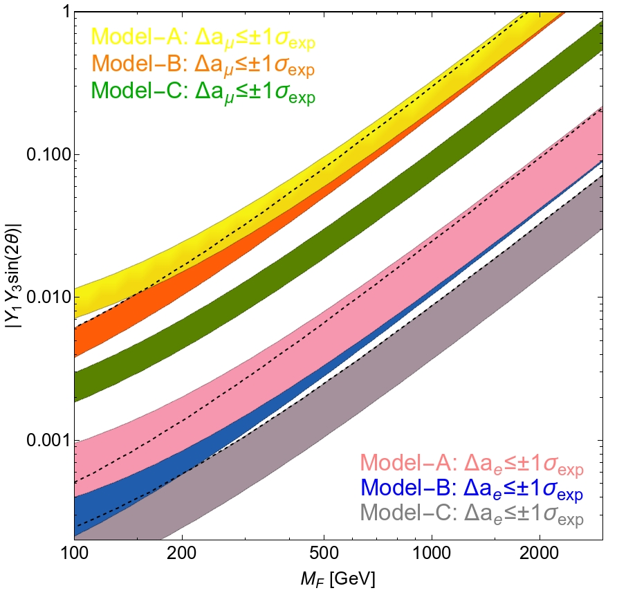
Figure 4: Demonstration of the required Yukawa coupling to reproduce the experimentally observed lepton AMMs within $1\sigma$ values are presented as a function of vector-like fermion mass $M_{F}$. For the masses of two of the scalars running in the loop, we take $M_{F}+100$ GeV and $M_{F}+150$ GeV, respectively. Here, for illustration, we have only plotted the dominant chiraly enhanced contribution; however, for numerical analysis, we have consider the full expressions.

Lepton magnetic dipole moment:– The NP contributions to lepton AMMs in this theory appear at the one-loop order, as shown in Fig. 3 (Feynman diagram on the bottom). These contributions are typically large due to vector-like fermion mass insertion in the loop. The outgoing photon in this Feynman diagram is emitted either by an internal scalar or fermion, or by both scalar and fermion, depending on the model. In Model-A, -B, and -C, scalars (fermions) running in the loop are singly-charged (neutral), neutral (singly-charged), and doubly-charged (singly-charged) states, respectively. It is straightforward to evaluate the contribution arising from BSM states, which yields,

$$\Delta a_{\ell} =-\frac{m_{\ell}}{4\pi^{2}}\bigg{\{}Re\left(Y^{L\ast}_{kl}Y^{R}_{kl}\right)\frac{M_{k}}{M^{2}_{S^{x}_{b}}}G[r_{kb}]$$

$$+\left(|Y^{L}_{kl}|^{2}+|Y^{R}_{kl}|^{2}\right)\frac{m_{\ell}}{M^{2}_{S^{x}_{b}}}\widetilde{G}[r_{kb}]\bigg{\}},$$ (33)

where summation over the BSM scalars and fermions must be understood. Furthermore, we have defined,

$$r_{kb}=\frac{M^{2}_{k}}{M^{2}_{S^{x}_{b}}},$$ (34)

$$G[r]=f[r]+Q_{\psi}g[r],$$ (35)

$$\widetilde{G}[r]=\widetilde{f}[r]+Q_{\psi}\widetilde{g}[r],$$ (36)

with $Q_{\psi}=0,-1,+1$ for Model-A, -B, -C, respectively, and,

$$f[r]=2\widetilde{g}[r]=\frac{r^{2}-1-2r\ln r}{4(r-1)^{3}},$$ (37)

$$g[r]=\frac{r-1-\ln r}{2(r-1)^{2}},$$ (38)

$$\widetilde{f}[r]=\frac{2r^{3}+3r^{2}-6r+1-6r^{2}\ln r}{24(r-1)^{4}}.$$ (39)

Finally, the re-defined Yukawa couplings $(Y^{\ast}_{L},Y_{R})$ appearing in Eq. (33) are given by,

$$\textrm{Model-A}:$$

$$\eta_{1}:(Y_{1}c_{\theta_{+}},Y_{3}s_{\theta_{+}}),\;\;\eta_{2}:(-Y_{1}s_{\theta_{+}},Y_{3}c_{\theta_{+}}),$$ (40)

$$\textrm{Model-B}:$$

$$S_{1}:(Y_{1}c_{\theta_{0}},Y_{3}s_{\theta_{0}}),\;\;S_{2}:(-Y_{1}s_{\theta_{0}},Y_{3}c_{\theta_{0}}),$$ (41)

$$\textrm{Model-C}:$$

$$\kappa_{1}:(Y_{1}c_{\theta_{++}},Y_{3}s_{\theta_{++}}),\;\;\kappa_{2}:(-Y_{1}s_{\theta_{++}},Y_{3}c_{\theta_{++}}).$$ (42)

In Fig. 4, we present beyond SM contributions to the muon and the electron anomalous magnetic moments arising in three versions of models under consideration. It is clear from this plot that the required large contributions as observed in the experiments can be naturally provided within this framework without requiring large Yukawa couplings. Furthermore, opposite signs of the muon and the electron AMMs can be incorporated via an appropriate choice of the signs of the associated Yukawa couplings.

IV Experimental constraints

This section briefly describes the phenomenological implications of the proposed models and the current experimental bounds on the BSM states, along with future collider prospects.

LHC bounds on scalars and fermions:– Model-A contains a DM candidate (see Sec. V for details) via which it can be tested in colliders. Specifically, the singly charged scalars can be efficiently pair-produced at the LHC through the $s$-channel $\gamma/Z$ exchange. Once pair-produced, each of them decays into a DM and a SM lepton, i.e., $pp\to\ell^{+}\ell^{-}+\not{E}_{T}$. This process mimics the standard slepton searches carried out by ATLAS as well as CMS collaborations Aad:2014yka ; Sirunyan:2018nwe ; Sirunyan:2018vig and non-observation of any such processes lead to a bound of $m_{S^{\pm}_{i}}\geq 450$ GeV Sirunyan:2018nwe .

On the contrary, Model-B/C does not contain a DM candidate. Consequently, collider probes of these models are distinct from Model-A. Following Model-A, we assume that BSM scalars are heavier than BSM fermionic states in Model-B/C. Then pair-produced singly (singly and doubly) charged scalars in Model-B (Model-C) decay into a pair of SM lepton ($\nu\nu$ or $\ell^{+}\ell^{-}$ depending on singly or doubly charged scalar) and a pair of BSM singly charged fermions ($\psi^{+}\psi^{-}$). In fact, the singly charged fermions also get pair-produced through the $s$-channel $\gamma/Z$ exchange, which provides the relevant bounds for these models. Note, however, that for a general charge assignment with an arbitrary value of $\beta$, a renormalizable coupling responsible for the decay of these fermions may not be present; hence $\psi^{\pm}$ are expected to be long-lived.

To make them decay, we fix the $B-L$ charge such that $\beta=-1$ for Model-B/C, therefore a mixing term of the form $\mathcal{L}\supset m^{\prime}\overline{\psi}_{L}\ell_{R}$ is allowed. Its contribution to SM lepton masses can be fully neglected if $\epsilon\ll 1$, where we define $m^{\prime}\equiv\epsilon v_{H}/\sqrt{2}$. Through this mixing, the vector-like leptons will promptly decay if $\epsilon\gtrsim 2\times 10^{-7}$ Bhattiprolu:2019vdu . For a quasi-stable vector-like lepton, assuming chargino like interactions, ATLAS search ATLAS:2019gqq provides a bound of $m_{\psi^{\pm}}\geq 750$ GeV Bhattiprolu:2019vdu . On the other hand, for the prompt decay scenario, each of the pair-produced vector-like lepton decays into $\psi\to h\ell$, $\psi\to Z\ell$, and $\psi\to W\nu_{\ell}$, for which currently there is no collider bound. However, HL-LHC (14 TeV with integrated luminosity of $3ab^{-1}$) will probe these processes and should be able to exclude up to about $m_{\psi^{\pm}}\geq 460$ GeV for the first two generations OsmanAcar:2021plv and $m_{\psi^{\pm}}\geq 600$ GeV for tau-like $\psi$ Bhattiprolu:2019vdu .

Electroweak precision constraints:– Neutrino mass and BSM contributions to the lepton anomalous magnetic moments heavily depend on the splitting between the neutral (and charged) BSM scalars; hence electroweak precision measurements provide stringent constraints on the model parameters. The so-called $T$-parameter is the most crucial among these oblique parameters, which we compute following Refs. Peskin:1990zt ; Barbieri:2006dq ; Grimus:2008nb ; Funk:2011ad and allow it to vary within the range given by ParticleDataGroup:2020ssz ,

$$\Delta T=0.03\pm 0.12.$$ (43)

LEP bounds on vector boson:– Since we study gauged $B-L$ extension of the SM, this theory contains a heavy gauge boson $Z^{\prime}$, which is significantly constrained from the non-observation of any direct signature at LEP and LHC. This gauge boson couples to quarks as well as leptons, thus $Z^{\prime}$ can be produced and searched for at the LEP via $s$-channel $e\overline{e}\to Z^{\prime}\to f\overline{f}$ processes. To assure LEP-II bound LEP:2003aa , we impose

$$\frac{M_{Z^{\prime}}}{g^{\prime}}>6.94\textrm{TeV at $95\%$ C.L.},$$ (44)

which is derived from effective four-lepton operator Carena:2004xs and valid for $M_{Z^{\prime}}\gg 200$ GeV.

LHC bounds on vector boson:– Furthermore, at hadron colliders, $Z^{\prime}$ can be efficiently produced in the $s$-channel due to its couplings to quarks, which would show up as resonances in the invariant mass distribution of the decay products. Searching for a massive resonance at the LHC decaying into di-lepton/di-jet imposes stringent limits on the respective production cross-section. The current data from 13 TeV LHC search for a heavy resonance decaying into two leptons (assuming a $100\%$ branching ratio) via $pp\to Z^{\prime}\to\ell^{+}\ell^{-}$ provides the tightest constraint of $M_{Z^{\prime}}>4.9$ TeV. This bound is somewhat relaxed for other branching ratios, which is depicted in Fig. 8 using the current data (ATLAS ATLAS:2019erb and CMS CMS:2021ctt ) and future projections (HL-LHC Ruhr:2016xsg and FCC-hh Helsens:2019bfw ) in the coupling versus mass plane Padhan:2022fak .

Cosmological constraints on vector boson:– Since neutrinos are Dirac particles in our scenario, the existence of right-handed neutrinos $\nu_{R}$ is implied. Since these right-handed neutrinos are mass degenerate with left-handed neutrinos $\nu_{L}$, they could contribute to the effective number of relativistic degrees of freedom $N_{eff}$ in the early Universe. In the case of purely SM interactions, the contributions are completely negligible. However, in our model, $\nu_{R}$ have gauge interactions with $Z^{\prime}$, through which they can be in thermal equilibrium with the SM plasma in the early Universe via $s$-channel $f\overline{f}\leftrightarrow\nu_{R}\overline{\nu}_{R}$ processes that increases $N_{eff}$. Cosmological data, however, requires that $\nu_{R}$s decouple from the SM plasma much earlier than the $\nu_{L}$. To be specific, Planck 2018 data Planck:2018nkj ; Planck:2018vyg requires that $\nu_{R}$s must decouple at temperatures greater than $T>0.6$ GeV Abazajian:2019oqj .

The best current measurement implies $N_{eff}=2.99\pm 0.17$ Planck:2018nkj ; Planck:2018vyg , which is in complete agreement with the SM prediction $N^{SM}_{eff}=3.045$ Mangano:2005cc ; Grohs:2015tfy ; deSalas:2016ztq . Then a $2\sigma$ C.L. corresponds to $\Delta N_{eff}<0.285$, which we adopt in our analysis. Future sensitives of CMB-S4 experiments will reach a precision of $\Delta N_{eff}\sim 0.03$ CMB-S4:2016ple ; Abazajian:2019eic that can probe NP scale up to about 50 TeV Abazajian:2019oqj ; Luo:2020sho . For heavy $Z^{\prime}$, i.e., $M_{Z^{\prime}}>20$ GeV, assuming that $\nu_{R}$ decouples before $T\sim 0.6$ GeV, one obtains $M_{Z^{\prime}}/g^{\prime}>11.4$ TeV, for the case of the standard $B-L$ theory Luo:2020sho (this limit becomes much stronger in the lower mass range, see, e.g., Ref. Abazajian:2019oqj ). We re-scale this bound using the unconventional charge assignment of the right-handed neutrinos in our theory, and the corresponding Planck 2018 bound is presented in Fig. 9.

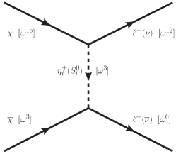
Figure 5: Dark matter annihilation into SM leptons.

V Dark Matter

In this theory, the Diracness of neutrinos is protected by the $U(1)_{B-L}$ symmetry. Remarkably, this same symmetry is also responsible for stabilizing the DM candidate. The spontaneous symmetry breaking of $U(1)_{B-L}$ by the VEV of $\sigma$ leaves a residual discrete symmetry $\mathcal{Z}_{D}$ (such that $\omega^{D}=1$) and stabilizes the DM. In particular, stability is guaranteed if $D>2$ as well as if $D$ is even Bonilla:2018ynb . In such a case, all SM fields transform as even powers of $\omega$, and the lightest particle transforming as an odd power of $\omega$ will be automatically stable. For concreteness, for Model-A, we fix $\beta=-1/2$ in our analysis, and the corresponding charges of all fields under the residual symmetry are presented in Table 2. As can be seen from this Table, all particles in the dark sector ($\psi,\phi,S^{0},\eta^{+}$) carry charges that are odd powers of $\omega$.

Fields	$U(1)_{B-L}$	$U(1)_{B-L}\to\mathcal{Z}_{18}$
$Q_{L},u_{R},d_{R}$	$\frac{1}{3}$	$\omega^{2}$
$L_{L},\ell_{R}$	$-1$	$\omega^{12}$
$\nu_{R}$	$-4,5$	$\omega^{12}$
$\psi$	$-\frac{1}{2}$	$\omega^{15}$
$H$	$0$	$\omega^{0}$
$\sigma$	$3$	$\omega^{0}$
$\phi^{\ast}$	$\frac{1}{2}$	$\omega^{3}$
$S^{0}$	$\frac{7}{2}$	$\omega^{3}$
$\eta^{+}$	$\frac{1}{2}$	$\omega^{3}$

Table 2: Charges of particles under the residual symmetry in Model-A with $\beta=-1/2$. The dark sector transforms as an odd power of $\omega$, whereas the rest of the particles transform as even powers of $\omega$. See text for details.

The physical states in the dark sector of the Model-A consists of three Dirac fermions: $\psi_{i},\,(i=1-3)$, two singly-charged scalars, $\eta_{i}$ and two complex neutral scalars, $S_{i}$ with $i=1,2$. The DM candidate is the lightest Dirac fermion, which we choose to be $\psi_{2}\equiv\chi$. A typical DM annihilation channel in our model is demonstrated in Fig. 5. Before delving into the thermal freeze-out scenario of the DM, we delineate the relevant parameter space and constraints set by the DM direct detection experiments.

DM Direct Detection and Parameter Space

DM Direct Detection:– The fermionic DM, being charged under $U(1)_{B-L}$, will scatter with the nucleon via the exchange of $Z^{\prime}$ at the tree-level, and in the limit of zero momentum transfer one can deduce the following effective interaction term in the Lagrangian between the DM and the nucleon,

$$-{\cal L}\supset\frac{g^{\prime 2}}{2M_{Z^{\prime}}^{2}}\overline{\chi}\gamma_{\mu}\chi\overline{N}\gamma^{\mu}N\;,$$ (45)

where, $N$ is the nucleon. The spin independent scattering cross-section associated with this effective interaction is given as,

$$\sigma_{\mathrm{SI}}=\frac{1}{4\pi}\frac{g^{\prime 4}\mu_{r}^{2}}{4M_{Z^{\prime}}^{4}}\;,$$ (46)

where, the reduced mass is $\mu_{r}=\frac{m_{N}M_{\mathrm{DM}}}{m_{N}+M_{\mathrm{DM}}}$, and the cross-section is insensitive to the DM mass. Consequently, for a fixed DM mass, the limits on the $\sigma_{\mathrm{SI}}$ set by the currently operating DM direct detection experiments will constrain the region of two dimensional $M_{Z^{\prime}}-g^{\prime}$ parameter plane as shown in Fig. 8.

DM Parameter Space:– We want to correlate the constraints on the electron and muon magnetic dipole moments with the parameter space associated with the DM relic density. Hence, based on the choice of the Yukawa matrices given in Eq. (12), and the scalar masses and mixing angles given in Eq. (20), we choose the parameter space for the DM relic density analysis which is spanned by $M_{\mathrm{DM}}$, $M_{F_{1}}$, $M_{\eta_{1}}$, $M_{\eta_{2}}$, $M_{S_{1}}$, $M_{S_{2}}$, $\theta_{+}$, $\theta_{0}$, $Y_{1_{ee}}$, $Y_{1_{\mu\mu}}$, $Y_{3_{ee}}$, $Y_{3_{\mu\mu}}$, $g^{\prime}$ and $M_{Z^{\prime}}$. Besides, the Yukawa couplings $Y_{2}$ being connected with the neutrino mass generation are much smaller than $Y_{1}$ and $Y_{3}$, and therefore don’t play any significant role in the DM relic density analysis.

DM Relic Density

We consider the standard thermal freeze-out to achieve the correct DM relic density, $\Omega h^{2}=0.12\pm 0.001$ ($68\%$ C.L.) observed by Planck Planck:2018vyg . The dominant (co)annihilation processes which control the DM relic density for our considered DM parameter space, where $Y_{1}$ and $Y_{3}$ Yukawa matrices being diagonal, are enumerated in the following.

• $\overline{\chi}\,\chi\rightarrow\mu^{+}\mu^{-}\,\,\mathrm{and}\,\,\overline{\nu}_{\mu}\nu_{\mu}$ via the exchange of $\eta^{+}_{1,2}$ and $S_{1,2}$ at the t-channel, respectively.

• $\overline{\chi}\,\chi\rightarrow\overline{q}q,\,l^{+}l^{-},\,\overline{\nu}_{l}\nu_{l}$ i.e. to the SM quark ($q$), charged lepton ($l$) and neutrino ($\nu_{l}$) pairs via the exchange of $Z^{\prime}$ at the s-channel.

When the mass splitting between the DM candidate and another dark sector particle carrying same dark charge is small, the coannihilation channels also become important. In our case, the dominant coannihilation channels involving the DM candidate $\chi$ and other dark sector particles: $\psi_{1}$, $\eta^{+}_{1,2}$ and $S_{1,2}$ are,

• $\chi\,\overline{\psi}_{1}\rightarrow\mu^{-}e^{+},\,\nu_{\mu}\overline{\nu}_{e}$, $\chi\,\eta^{-}_{1,2},\,\chi\,S^{*}_{1,2}\rightarrow\overline{X^{\prime}}X$ where $X,\,X^{\prime}$ are the SM particles, and the conjugated channels.

• $\psi_{1}\,\eta^{-}_{1,2},\,\psi_{1}S^{*}_{1,2},\,\eta^{+}_{i}\,\eta^{-}_{j},\,S_{i}\,S^{*}_{j},\,\eta^{+}_{i}\,S^{*}_{j}\rightarrow\overline{X^{\prime}}X$ where $i,\,j=1,\,2$, and the relevant conjugated channels.

As the DM relic density involves multiple (co)annihilation channels, which also depend on the multi-dimensional parameter space, we consider two scenarios to capture the dynamics in a simplified manner. First, we consider the mass of the $Z^{\prime}$ quite heavy compared to DM and other BSM particles so that the contribution of the $Z^{\prime}$ mediated channels in the thermal freeze-out become negligible. We call it the $Z^{\prime}$ decoupled scenario, and in this case, the thermal freeze-out of the DM is controlled by the BSM Yukawa sector of the Model-A. In the second scenario, dubbed here as BSM Yukawa + $Z^{\prime}$ gauge boson scenario, we take into account both the simultaneous contributions of the BSM Yukawa sector and the $Z^{\prime}$ gauge bosons to determine the DM relic density.

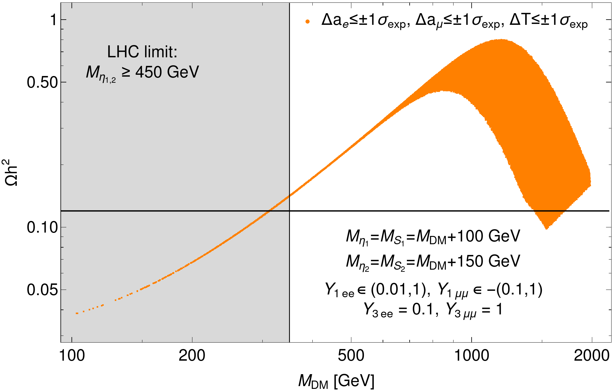
Figure 6: The correlation between the mass of the DM candidate $F_{2}$, $M_{DM}$ and the DM relic density $\Omega h^{2}$ for the parameter space which satisfy the constraints on the electron and muon magnetic moments, $\Delta a_{e}$ and $\Delta a_{\mu}$ and T-parameter $\Delta T$ for the $Z^{\prime}$ decoupled scenario. The black horizontal line represents the correct DM relic density determined by Planck.

$Z^{\prime}$ decoupled scenario:– Although we consider the $Z^{\prime}$ contribution to be negligible in determining the DM relic density for this scenario as mentioned above, the relevant parameter space is still large enough to disentangle the effects of the BSM Yukawa couplings, $Y_{1}$ and $Y_{3}$, the mass-splittings between the DM and the charged scalars $\eta_{1,2}^{+}$ and neutral scalars $S_{1,2}$, and the scalar mixing angles $\theta_{+}$ and $\theta_{0}$ on the DM relic density concretely just by scanning over the parameters randomly. Therefore, we consider a few benchmark points of the parameter space and discuss the impact of the variations of the parameters on the DM relic density.

First we consider a benchmark point where we fixed the following parameters as follows,

$$M_{F_{1}}=M_{DM}+1\,\mathrm{GeV},\,M_{\eta_{1}}=M_{S_{1}}=M_{DM}+100\,\mathrm{GeV},$$

$$M_{\eta_{2}}=M_{S_{2}}=M_{DM}+150\,\mathrm{GeV},\,\theta_{+}=\theta_{0}=0.7,$$

$$Y_{3_{ee}}=0.1,\,Y_{3_{\mu\mu}}=1,$$ (47)

and vary only the Yukawa couplings, $Y_{1_{ee}}\in(0.01,1)$ and $Y_{1_{\mu\mu}}\in-(0.1,1)$ randomly to select the points which simultaneously satisfy the constraints on the electron and muon magnetic moments $\Delta a_{e}$ and $\Delta a_{\mu}$ and T-parameter $\Delta T$. Afterwards, we calculate the relic density of the DM $F_{2}$ for each of these selected points using micrOMEGAsv$5.2$ Belanger:2020gnr with the model files generated by FeynRules Alloul:2013bka .

  

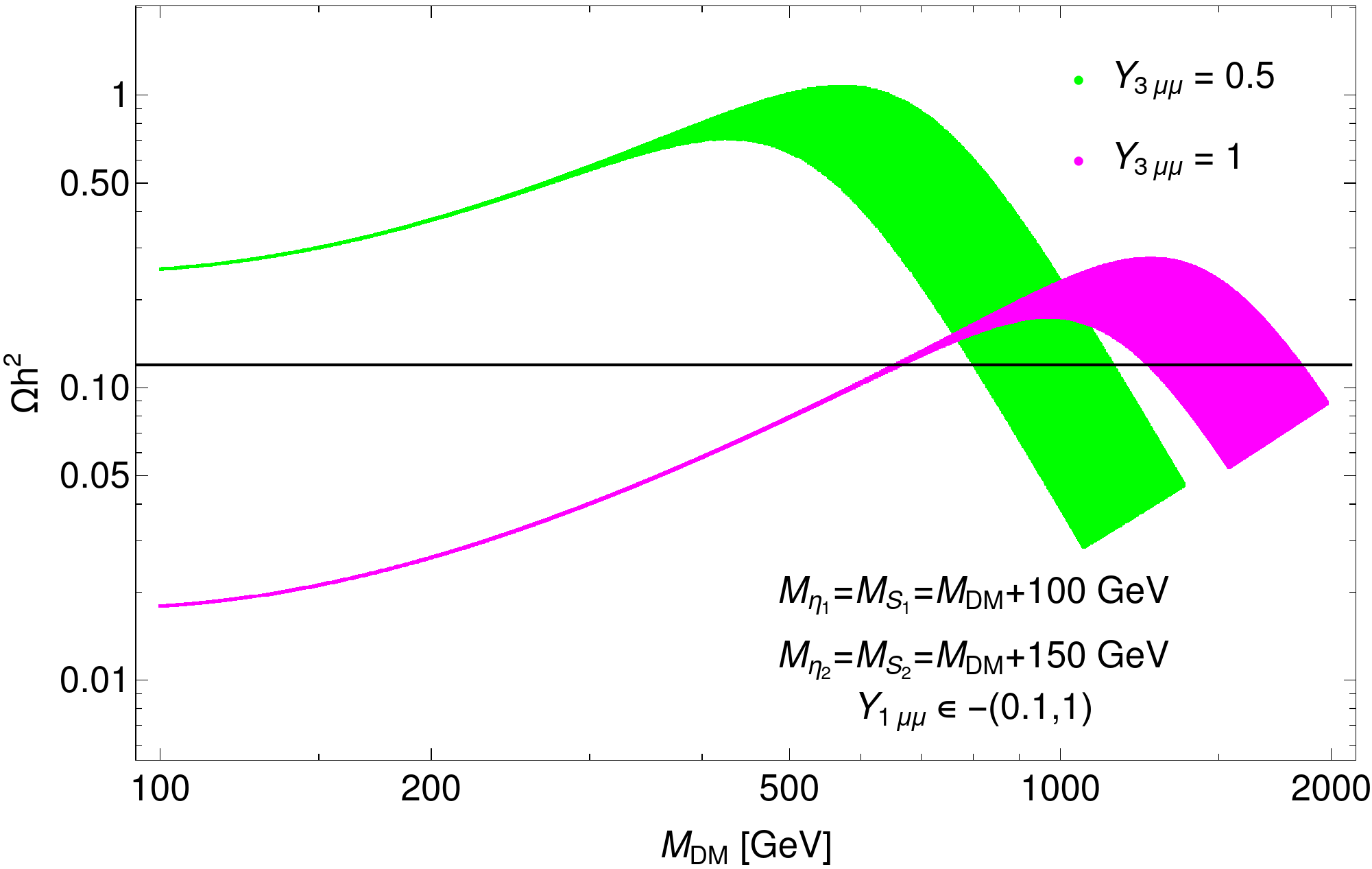
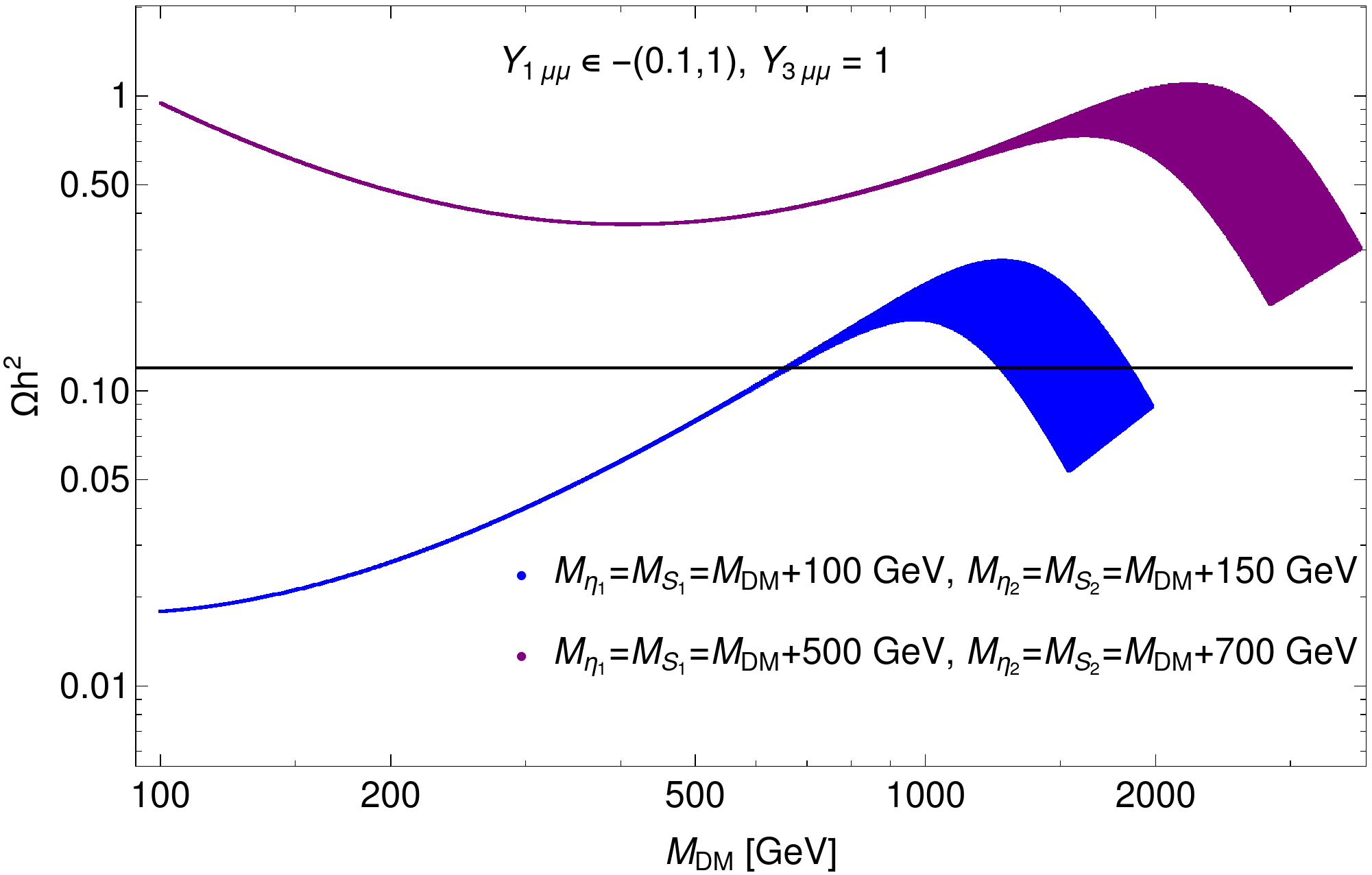
Figure 7: The dependence of the DM relic density on the variation of $Y_{3_{\mu\mu}}$ for a fixed mass splitting (left fig.) and on the mass splittings between the DM and charged and neutral scalars for a fixed value of $Y_{3_{\mu\mu}}$ (right fig.). Here we vary $Y_{1_{\mu\mu}}\in-(0.1,1)$. For simplicity, in this presentation, we only consider the parameter points satisfying the constraints on the muon magnetic moment $\Delta a_{\mu}$ and the T parameter $\Delta T$ simultaneously. Again the black horizontal line represents the correct DM relic density. The respective collider bounds are not shown in this plots, see text for details.

Subsequently, for the parameter set given in Eq. (47), the correct DM relic density is obtained for $M_{DM}=310$ GeV which is excluded by the LHC limits, and for $1.4-1.7$ TeV mass range as seen in Fig. 6. To illustrate it, first, we write down the representative annihilation cross-section at low-velocity approximation that is associated with the DM, $\chi$ annihilating into the SM leptons (charged and neutrinos) via the exchange of charged ($\eta_{1,2}$) and neutral ($S_{1,2}$) scalars at t-channel,

$$\sigma v_{0}=\frac{M_{DM}^{2}\left(\tilde{Y}^{2}_{1_{a}}+\tilde{Y}^{2}_{3_{a}}\right)^{2}}{32\pi\left(M_{DM}^{2}+M_{\tilde{S}_{i}}^{2}\right)^{2}}\;,$$ (48)

where the terms having small masses of the final-state leptons are neglected, and $\tilde{Y}_{1_{a}}$ and $\tilde{Y}_{3_{a}}$ are the Yukawa couplings of electron or muon sector (here denoted by $a$) redefined by absorbing the appropriate scalar mixing angles associated with charged or neutral scalar (here expressed with $\tilde{S}_{i}$). As we choose $Y_{3_{\mu\mu}}=1$ for our parameter set in Eq. (47), when the DM mass is in $100-680$ GeV range, the term like $\tilde{Y}_{3_{\mu\mu}}^{4}M_{DM}^{2}$ in the numerator of Eq. (48) dominates the cross-section, and therefore we see the narrow band for that mass range. In contrast, when $M_{DM}>680$ GeV, the DM mass is large enough to make the terms like $\tilde{Y}_{1_{\mu\mu}}^{4}M_{DM}^{2}$ in the numerator of Eq. 48 also comparable to the terms with $Y_{3_{\mu\mu}}$, and thus we see the band at larger masses in the DM relic density plot as $|Y_{1_{\mu\mu}}|$ takes value in the range $(0.1,1)$. Besides, as the mass-splittings are small ($150$ GeV) when the DM mass is close to $O(\mathrm{TeV})$, the coannihilation channels also contribute significantly to the DM relic density, so the simplified Eq. 48 is not applicable for higher DM mass ranges with small mass-splittings.

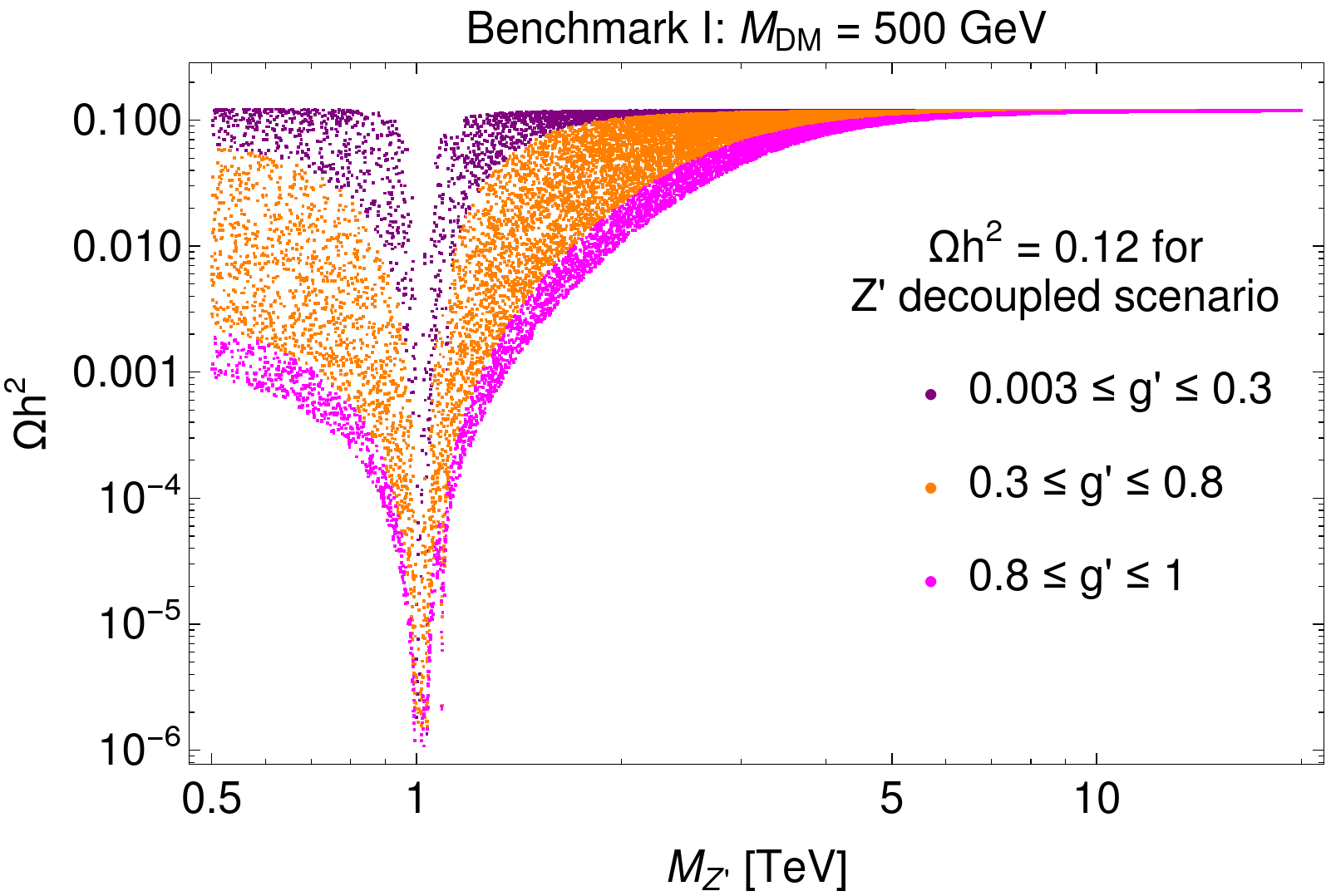
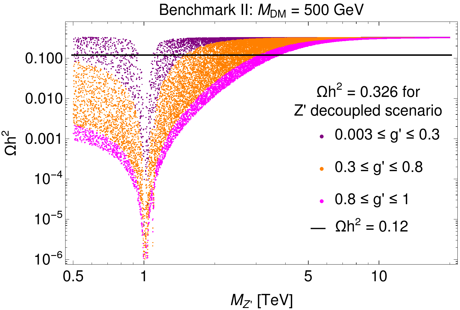
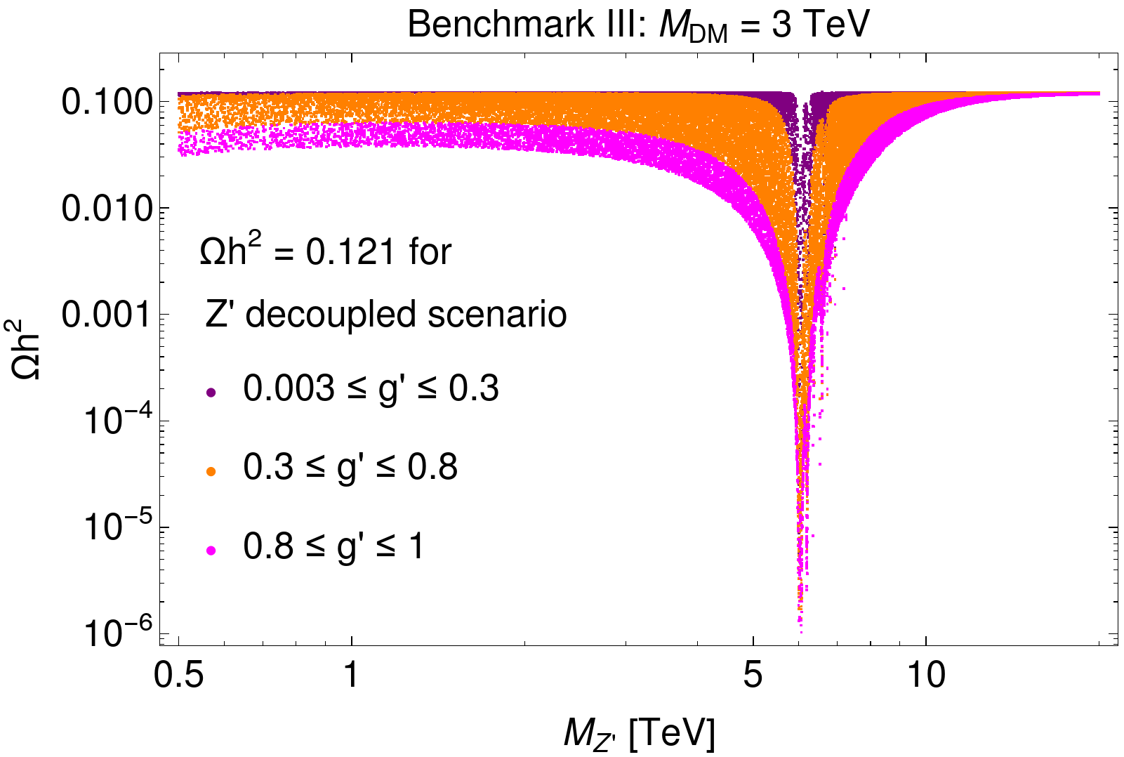
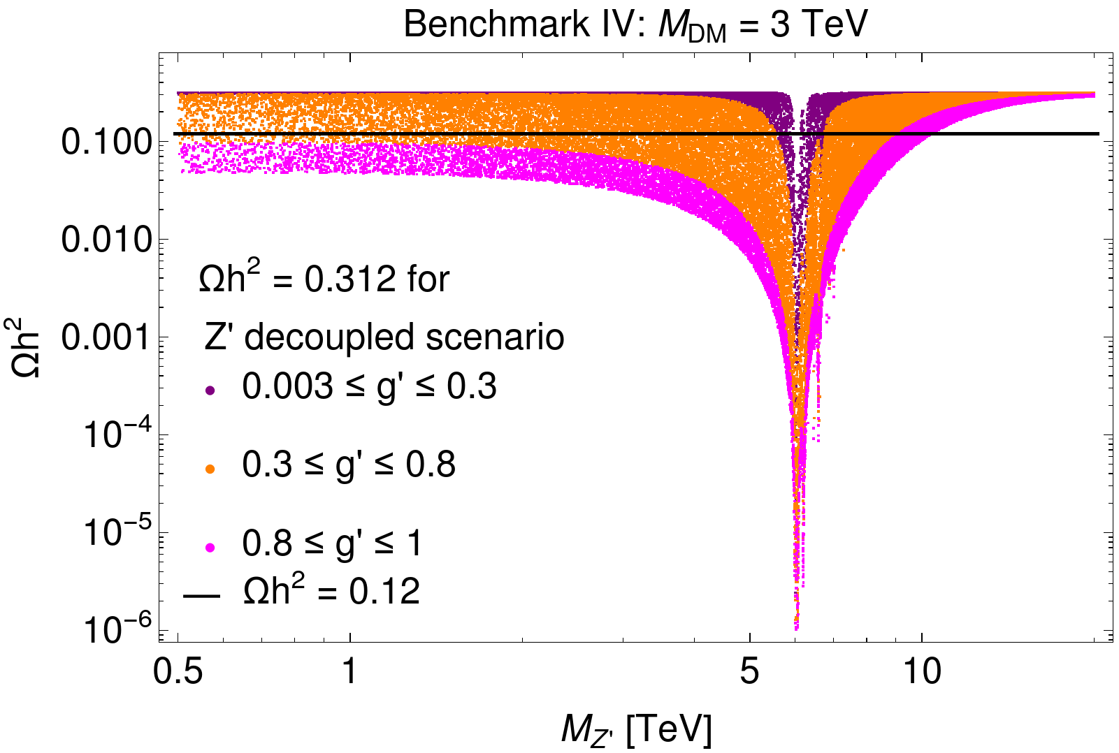
Figure 8: Correlation between the mass of the $Z^{\prime}$ gauge boson $M_{Z^{\prime}}$ and the DM relic density $\Omega h^{2}$ for four benchmark points given in Table 3.

In Fig. 7 (left), we can see that if $Y_{3_{\mu\mu}}$ is set to 0.5 instead of 1, the annihilation cross-section decreases for a wide range of the DM mass, and for this reason, the DM relic density remains overabundant for DM mass close to TeV scale as opposed to the case with $Y_{3_{\mu\mu}}=1$ for which it remains underabundant for similar DM mass range. In addition, when we increase the mass-splittings between the DM and the charged and neutral scalars, for lower mass range, the denominator in Eq. 48 becomes more significant, and the annihilation cross-section decreases, which results in the overabundant DM. Besides, larger mass-splittings suppress the coannihilation processes during the thermal freeze-out resulting in the overabundance of the DM for masses in the TeV range.

Furthermore, to capture the impact of $Z^{\prime}$ on the DM relic density, first, we consider four benchmark points presented in Table. 3 which simultaneously satisfy the constraints on the electron and muon magnetic moments $\Delta a_{e}$ and $\Delta a_{\mu}$ and T-parameter $\Delta T$ in the $Z^{\prime}$ decoupled scenario.

Benchmark	$M_{F_{2}}$	$M_{F_{1}}$	$M_{\eta_{1}}$	$M_{\eta_{2}}$	$M_{S_{1}}$	$M_{S_{2}}$	$\theta_{+}$	$\theta_{0}$	$Y_{1_{ee}}$	$Y_{1_{\mu\mu}}$	$Y_{3_{ee}}$	$Y_{3_{\mu\mu}}$	$\Omega h^{2}$
I	500 GeV	501 GeV	961.46 GeV	1357.04 GeV	858.75 GeV	1085.4 GeV	0.05	0.56	0.09	-1.33	0.67	0.36	0.12
II	500 GeV	501 GeV	1008.3 GeV	1983.3 GeV	979.83 GeV	1408 GeV	0.04	0.02	0.09	-1.07	0.3	0.54	0.326
III	3000 GeV	3001 GeV	3160.5 GeV	3582 GeV	3077 GeV	3672.2 GeV	0.42	0.41	0.09	-0.96	0.78	0.73	0.121
IV	3000 GeV	3001 GeV	3124.6 GeV	3562 GeV	3205.6 GeV	3611.4 GeV	0.6	0.46	0.06	-1.11	0.84	0.45	0.312

Table 3: Benchmark points in the $Z^{\prime}$ decoupled scenario for $M_{DM}=500$ GeV and $M_{DM}=3000$ GeV.

For benchmark point I and II of Table 3 with $M_{DM}=500$ GeV, the thermal freeze-out of the DM is dominated by the processes, $\overline{\chi}\chi\rightarrow\overline{\nu}_{\mu}\nu_{\mu},\,\mu^{+}\mu^{-}$. On the other hand, for benchmark point III and IV with $M_{DM}=3000$ GeV, the thermal freeze-out processes are dominated by the coannihilation, for example, by $S_{1}S^{*}_{1}\rightarrow W^{+}W^{-},\,Z\,Z$ and $\eta^{+}_{1}\eta^{-}_{1}\rightarrow W^{+}W^{-},\,Z\,Z$, respectively.

BSM Yukawa sector + $Z^{\prime}$ gauge boson:– Now we calculate the DM relic density for the each benchmark points in Table 3 by varying the mass of the $Z^{\prime}$ gauge boson $M_{Z^{\prime}}\in(0.5,20)$ TeV and the gauge coupling $g^{\prime}\in(0.02,1)$.

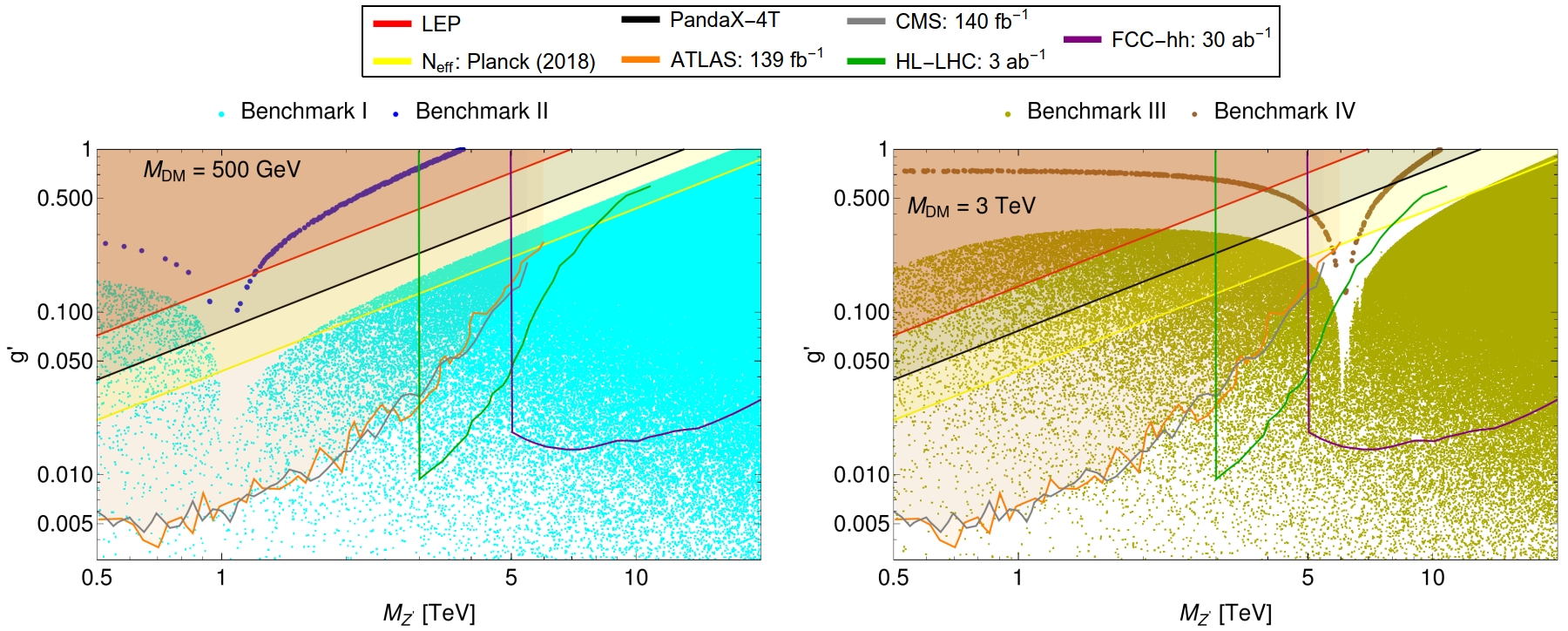
Figure 9: Correlation between $M_{Z^{\prime}}$ and $g^{\prime}$ for four benchmark points. For $m_{DM}=500$ GeV (left fig.), the cyan and blue points correspond to $(M_{Z^{\prime}},\,g^{\prime})$ pairs that satisfy the constraints on DM relic density for benchmark I and benchmark II points in the $Z^{\prime}$ decoupled scenario, respectively, whereas for $m_{DM}=3$ TeV (right fig.), the yellow-green and brown points represent those with same attribute for benchmark III and benchmark IV points, respectively. The shaded regions are ruled out by current collider bounds, cosmological constraints, and from dark matter direct detection. Future colliders will probe regions inside green and purple lines (not shaded).

From Fig. 8, we can see that for a fixed $M_{Z^{\prime}}$, the increase of the gauge coupling $g^{\prime}$ decreases the DM relic abundance determined in the $Z^{\prime}$ decoupled scenario. Therefore, even if the BSM Yukawa sector sets an overabundant DM relic density, one can achieve its observed value by adjusting the $Z^{\prime}$ mass and coupling $g^{\prime}$ as seen in Fig. 8 (upper and lower right figures). Moreover, we can see that the lower the value of the gauge coupling $g^{\prime}$, the lower the minimum value of the $M_{Z^{\prime}}$ where the $Z^{\prime}$’s contribution to the DM relic abundance becomes negligible. Besides, we see the dip in the DM relic abundance due to the resonant enhancement of DM annihilation processes involving the exchange of $Z^{\prime}$ at the s-channel when $M_{Z^{\prime}}\sim 2M_{DM}$.

In Fig. 9, we present the correlation between $M_{Z^{\prime}}$ and $g^{\prime}$ for our four benchmark points with all relevant constraints set by the collider searches and DM direct detection experiments, the observed DM relic density, and cosmological limit on the extra radiation. By correlating the Figs. 8 (upper left and right) and Fig. 9 (left), for $M_{DM}=500$ GeV, we see that the current limits provided by ATLAS and CMS have already ruled out the $(M_{Z^{\prime}},\,g^{\prime})$ values for which the $Z^{\prime}$ gauge boson give significant contributions to the DM relic abundance. Again the close inspection of Figs. 8 (lower left and right) and Fig. 9 (right) for $m_{DM}=3$ TeV indicates that apart from the small parameter space close to the resonance point around $M_{Z^{\prime}}\sim 6$ TeV, almost all the $(M_{Z^{\prime}},\,g^{\prime})$ values are ruled out by LEP, LHC, DM direct detection (e.g. PandaX-4T PandaX-4T:2021bab which has set the most stringent limit on the spin independent DM-nucleon cross-section for 10 GeV - 10 TeV DM mass range), and Planck constraint on $\mathrm{N}_{\mathrm{eff}}$. Furthermore, rest of the parameter space where $Z^{\prime}$ contributions could play an important role in determining DM relic abundance will be fully probed by the HL-LHC and future collider like FCC-hh.

Since the DM particle is inducing the anomalous magnetic dipole moment via mass-insertion, the chirality flip enhancement is strongly correlated to the mass generation mechanism of the associated lepton and causes related loop contributions to its mass. Hence, if $M_{DM}\gtrsim\mathcal{O}(3)$ TeV, typically, fine-turning of a large degree is required to adjust the lepton mass correctly. For details, see, e.g., Athron:2021iuf and references therein. This is why in this work, we explored DM phenomenology in the range $100\,\mathrm{GeV}\stackrel{{\scriptstyle<}}{{{}_{\sim}}}M_{DM}\stackrel{{\scriptstyle<}}{{{}_{\sim}}}3$ TeV.

VI Conclusion

The Fermilab’s Muon $g-2$ experiment has recently confirmed the longstanding tension of the muon AMM. Furthermore, the recent precise measurement of the electron AMM at the Berkeley Lab shows deviations from the theoretical prediction. These two anomalies together strongly hint towards physics beyond the Standard Model. Besides, the origin of neutrino mass remains a mystery even after the groundbreaking discovery of neutrino oscillation about twenty-five years ago. Moreover, even though we know DM exists, we do not yet know what it is at a fundamental level.

This work proposes a class of radiative Dirac neutrino mass models where neutrino mass arises at a one-loop level. Furthermore, NP states that participate in neutrino mass generation also run through the loops and significantly contribute to $(g-2)_{\mu,e}$. These large contributions arise due to chirality enhancements required to simultaneously explain the $(g-2)_{\mu}$ and $(g-2)_{e}$ data. For completeness, we have studied three benchmark models, one of which (Model-A) offers a Dark Matter candidate whose stability is naturally protected without imposing additional symmetries by hand. For Model-A, we have performed a detailed numerical analysis to investigate the correlations among the common model parameters accommodating neutrino oscillation data, the muon, the electron g-2, and dark matter relic abundance. Parameters that generate non-zero neutrino mass also play a non-trivial role in explaining the muon and the electron $g-2$ simultaneously; furthermore, these same parameters take part in dark matter annihilations to the SM particles in reproducing the correct relic abundance. This model is subject to numerous constraints arising from colliders and cosmology, through which it can be probed in the current and upcoming experiments. A detailed study of lepton flavor violation and electric dipole moments of the electron and the muon and their possible links to the puzzles resolved in this work is left for future work.

References

- (1) Muon g-2 Collaboration, G. W. Bennett et al., “Final Report of the Muon E821 Anomalous Magnetic Moment Measurement at BNL,” Phys. Rev. D73 (2006) 072003, arXiv:hep-ex/0602035 [hep-ex].
- (2) Muon g-2 Collaboration, B. Abi et al., “Measurement of the Positive Muon Anomalous Magnetic Moment to 0.46 ppm,” Phys. Rev. Lett. 126 no. 14, (2021) 141801, arXiv:2104.03281 [hep-ex].
- (3) T. Aoyama et al., “The anomalous magnetic moment of the muon in the Standard Model,” Phys. Rept. 887 (2020) 1–166, arXiv:2006.04822 [hep-ph].
- (4) T. Aoyama, M. Hayakawa, T. Kinoshita, and M. Nio, “Complete Tenth-Order QED Contribution to the Muon g-2,” Phys. Rev. Lett. 109 (2012) 111808, arXiv:1205.5370 [hep-ph].
- (5) T. Aoyama, T. Kinoshita, and M. Nio, “Theory of the Anomalous Magnetic Moment of the Electron,” Atoms 7 no. 1, (2019) 28.
- (6) A. Czarnecki, W. J. Marciano, and A. Vainshtein, “Refinements in electroweak contributions to the muon anomalous magnetic moment,” Phys. Rev. D 67 (2003) 073006, arXiv:hep-ph/0212229. [Erratum: Phys.Rev.D 73, 119901 (2006)].
- (7) C. Gnendiger, D. Stöckinger, and H. Stöckinger-Kim, “The electroweak contributions to after the Higgs boson mass measurement,” Phys. Rev. D 88 (2013) 053005, arXiv:1306.5546 [hep-ph].
- (8) M. Davier, A. Hoecker, B. Malaescu, and Z. Zhang, “Reevaluation of the hadronic vacuum polarisation contributions to the Standard Model predictions of the muon and using newest hadronic cross-section data,” Eur. Phys. J. C 77 no. 12, (2017) 827, arXiv:1706.09436 [hep-ph].
- (9) A. Keshavarzi, D. Nomura, and T. Teubner, “Muon and : a new data-based analysis,” Phys. Rev. D 97 no. 11, (2018) 114025, arXiv:1802.02995 [hep-ph].
- (10) G. Colangelo, M. Hoferichter, and P. Stoffer, “Two-pion contribution to hadronic vacuum polarization,” JHEP 02 (2019) 006, arXiv:1810.00007 [hep-ph].
- (11) M. Hoferichter, B.-L. Hoid, and B. Kubis, “Three-pion contribution to hadronic vacuum polarization,” JHEP 08 (2019) 137, arXiv:1907.01556 [hep-ph].
- (12) M. Davier, A. Hoecker, B. Malaescu, and Z. Zhang, “A new evaluation of the hadronic vacuum polarisation contributions to the muon anomalous magnetic moment and to ,” Eur. Phys. J. C 80 no. 3, (2020) 241, arXiv:1908.00921 [hep-ph]. [Erratum: Eur.Phys.J.C 80, 410 (2020)].
- (13) A. Keshavarzi, D. Nomura, and T. Teubner, “ of charged leptons, , and the hyperfine splitting of muonium,” Phys. Rev. D 101 no. 1, (2020) 014029, arXiv:1911.00367 [hep-ph].
- (14) A. Kurz, T. Liu, P. Marquard, and M. Steinhauser, “Hadronic contribution to the muon anomalous magnetic moment to next-to-next-to-leading order,” Phys. Lett. B 734 (2014) 144–147, arXiv:1403.6400 [hep-ph].
- (15) K. Melnikov and A. Vainshtein, “Hadronic light-by-light scattering contribution to the muon anomalous magnetic moment revisited,” Phys. Rev. D 70 (2004) 113006, arXiv:hep-ph/0312226.
- (16) P. Masjuan and P. Sanchez-Puertas, “Pseudoscalar-pole contribution to the : a rational approach,” Phys. Rev. D 95 no. 5, (2017) 054026, arXiv:1701.05829 [hep-ph].
- (17) G. Colangelo, M. Hoferichter, M. Procura, and P. Stoffer, “Dispersion relation for hadronic light-by-light scattering: two-pion contributions,” JHEP 04 (2017) 161, arXiv:1702.07347 [hep-ph].
- (18) M. Hoferichter, B.-L. Hoid, B. Kubis, S. Leupold, and S. P. Schneider, “Dispersion relation for hadronic light-by-light scattering: pion pole,” JHEP 10 (2018) 141, arXiv:1808.04823 [hep-ph].
- (19) A. Gérardin, H. B. Meyer, and A. Nyffeler, “Lattice calculation of the pion transition form factor with Wilson quarks,” Phys. Rev. D 100 no. 3, (2019) 034520, arXiv:1903.09471 [hep-lat].
- (20) J. Bijnens, N. Hermansson-Truedsson, and A. Rodríguez-Sánchez, “Short-distance constraints for the HLbL contribution to the muon anomalous magnetic moment,” Phys. Lett. B 798 (2019) 134994, arXiv:1908.03331 [hep-ph].
- (21) G. Colangelo, F. Hagelstein, M. Hoferichter, L. Laub, and P. Stoffer, “Longitudinal short-distance constraints for the hadronic light-by-light contribution to with large- Regge models,” JHEP 03 (2020) 101, arXiv:1910.13432 [hep-ph].
- (22) T. Blum, N. Christ, M. Hayakawa, T. Izubuchi, L. Jin, C. Jung, and C. Lehner, “Hadronic Light-by-Light Scattering Contribution to the Muon Anomalous Magnetic Moment from Lattice QCD,” Phys. Rev. Lett. 124 no. 13, (2020) 132002, arXiv:1911.08123 [hep-lat].
- (23) G. Colangelo, M. Hoferichter, A. Nyffeler, M. Passera, and P. Stoffer, “Remarks on higher-order hadronic corrections to the muon g2,” Phys. Lett. B 735 (2014) 90–91, arXiv:1403.7512 [hep-ph].
- (24) R. H. Parker, C. Yu, W. Zhong, B. Estey, and H. Müller, “Measurement of the fine-structure constant as a test of the Standard Model,” Science 360 (2018) 191, arXiv:1812.04130 [physics.atom-ph].
- (25) T. Aoyama, T. Kinoshita, and M. Nio, “Revised and Improved Value of the QED Tenth-Order Electron Anomalous Magnetic Moment,” Phys. Rev. D97 no. 3, (2018) 036001, arXiv:1712.06060 [hep-ph].
- (26) G. F. Giudice, P. Paradisi, and M. Passera, “Testing new physics with the electron g-2,” JHEP 11 (2012) 113, arXiv:1208.6583 [hep-ph].
- (27) H. Davoudiasl and W. J. Marciano, “Tale of two anomalies,” Phys. Rev. D98 no. 7, (2018) 075011, arXiv:1806.10252 [hep-ph].
- (28) A. Crivellin, M. Hoferichter, and P. Schmidt-Wellenburg, “Combined explanations of and implications for a large muon EDM,” Phys. Rev. D98 no. 11, (2018) 113002, arXiv:1807.11484 [hep-ph].
- (29) J. Liu, C. E. M. Wagner, and X.-P. Wang, “A light complex scalar for the electron and muon anomalous magnetic moments,” JHEP 03 (2019) 008, arXiv:1810.11028 [hep-ph].
- (30) B. Dutta and Y. Mimura, “Electron with flavor violation in MSSM,” Phys. Lett. B790 (2019) 563–567, arXiv:1811.10209 [hep-ph].
- (31) X.-F. Han, T. Li, L. Wang, and Y. Zhang, “Simple interpretations of lepton anomalies in the lepton-specific inert two-Higgs-doublet model,” Phys. Rev. D99 no. 9, (2019) 095034, arXiv:1812.02449 [hep-ph].
- (32) A. Crivellin and M. Hoferichter, “Combined explanations of , and implications for a large muon EDM,” in 33rd Rencontres de Physique de La Vallée d’Aoste (LaThuile 2019) La Thuile, Aosta, Italy, March 10-16, 2019. 2019. arXiv:1905.03789 [hep-ph].
- (33) M. Endo and W. Yin, “Explaining electron and muon anomaly in SUSY without lepton-flavor mixings,” JHEP 08 (2019) 122, arXiv:1906.08768 [hep-ph].
- (34) M. Abdullah, B. Dutta, S. Ghosh, and T. Li, “ and the ANITA anomalous events in a three-loop neutrino mass model,” Phys. Rev. D100 no. 11, (2019) 115006, arXiv:1907.08109 [hep-ph].
- (35) M. Bauer, M. Neubert, S. Renner, M. Schnubel, and A. Thamm, “Axion-like particles, lepton-flavor violation and a new explanation of and ,” arXiv:1908.00008 [hep-ph].
- (36) M. Badziak and K. Sakurai, “Explanation of electron and muon g - 2 anomalies in the MSSM,” JHEP 10 (2019) 024, arXiv:1908.03607 [hep-ph].
- (37) G. Hiller, C. Hormigos-Feliu, D. F. Litim, and T. Steudtner, “Anomalous magnetic moments from asymptotic safety,” arXiv:1910.14062 [hep-ph].
- (38) A. E. Cárcamo Hernández, S. F. King, H. Lee, and S. J. Rowley, “Is it possible to explain the muon and electron in a model?,” arXiv:1910.10734 [hep-ph].
- (39) C. Cornella, P. Paradisi, and O. Sumensari, “Hunting for ALPs with Lepton Flavor Violation,” arXiv:1911.06279 [hep-ph].
- (40) M. Endo, S. Iguro, and T. Kitahara, “Probing flavor-violating ALP at Belle II,” arXiv:2002.05948 [hep-ph].
- (41) A. E. Cárcamo Hernández, Y. H. Velásquez, S. Kovalenko, H. N. Long, N. A. Pérez-Julve, and V. V. Vien, “Fermion masses and mixings and anomalies in a low scale 3-3-1 model,” arXiv:2002.07347 [hep-ph].
- (42) N. Haba, Y. Shimizu, and T. Yamada, “Muon and Electron and the Origin of Fermion Mass Hierarchy,” arXiv:2002.10230 [hep-ph].
- (43) I. Bigaran and R. R. Volkas, “Getting chirality right: Single scalar leptoquark solutions to the puzzle,” Phys. Rev. D 102 no. 7, (2020) 075037, arXiv:2002.12544 [hep-ph].
- (44) S. Jana, V. P. K., and S. Saad, “Resolving electron and muon within the 2HDM,” Phys. Rev. D 101 no. 11, (2020) 115037, arXiv:2003.03386 [hep-ph].
- (45) L. Calibbi, M. L. López-Ibáñez, A. Melis, and O. Vives, “Muon and electron and lepton masses in flavor models,” JHEP 06 (2020) 087, arXiv:2003.06633 [hep-ph].
- (46) C.-H. Chen and T. Nomura, “Electron and muon , radiative neutrino mass, and in a model,” Nucl. Phys. B 964 (2021) 115314, arXiv:2003.07638 [hep-ph].
- (47) J.-L. Yang, T.-F. Feng, and H.-B. Zhang, “Electron and muon in the B-LSSM,” J. Phys. G 47 no. 5, (2020) 055004, arXiv:2003.09781 [hep-ph].
- (48) C. Hati, J. Kriewald, J. Orloff, and A. M. Teixeira, “Anomalies in 8Be nuclear transitions and : towards a minimal combined explanation,” JHEP 07 (2020) 235, arXiv:2005.00028 [hep-ph].
- (49) B. Dutta, S. Ghosh, and T. Li, “Explaining , the KOTO anomaly and the MiniBooNE excess in an extended Higgs model with sterile neutrinos,” Phys. Rev. D 102 no. 5, (2020) 055017, arXiv:2006.01319 [hep-ph].
- (50) F. J. Botella, F. Cornet-Gomez, and M. Nebot, “Electron and muon anomalies in general flavour conserving two Higgs doublets models,” Phys. Rev. D 102 no. 3, (2020) 035023, arXiv:2006.01934 [hep-ph].
- (51) K.-F. Chen, C.-W. Chiang, and K. Yagyu, “An explanation for the muon and electron anomalies and dark matter,” JHEP 09 (2020) 119, arXiv:2006.07929 [hep-ph].
- (52) I. Doršner, S. Fajfer, and S. Saad, “ selecting scalar leptoquark solutions for the puzzles,” Phys. Rev. D 102 no. 7, (2020) 075007, arXiv:2006.11624 [hep-ph].
- (53) C. Arbeláez, R. Cepedello, R. M. Fonseca, and M. Hirsch, “ anomalies and neutrino mass,” Phys. Rev. D 102 no. 7, (2020) 075005, arXiv:2007.11007 [hep-ph].
- (54) S. Jana, P. K. Vishnu, W. Rodejohann, and S. Saad, “Dark matter assisted lepton anomalous magnetic moments and neutrino masses,” Phys. Rev. D102 no. 7, (2020) 075003, arXiv:2008.02377 [hep-ph].
- (55) C.-K. Chua, “Data-driven study of the implications of anomalous magnetic moments and lepton flavor violating processes of , and ,” Phys. Rev. D 102 no. 5, (2020) 055022, arXiv:2004.11031 [hep-ph].
- (56) E. J. Chun and T. Mondal, “Explaining anomalies in two Higgs doublet model with vector-like leptons,” JHEP 11 (2020) 077, arXiv:2009.08314 [hep-ph].
- (57) S.-P. Li, X.-Q. Li, Y.-Y. Li, Y.-D. Yang, and X. Zhang, “Power-aligned 2HDM: a correlative perspective on ,” JHEP 01 (2021) 034, arXiv:2010.02799 [hep-ph].
- (58) L. Delle Rose, S. Khalil, and S. Moretti, “Explaining electron and muon 2 anomalies in an Aligned 2-Higgs Doublet Model with right-handed neutrinos,” Phys. Lett. B 816 (2021) 136216, arXiv:2012.06911 [hep-ph].
- (59) K. Kowalska and E. M. Sessolo, “Minimal models for g-2 and dark matter confront asymptotic safety,” Phys. Rev. D 103 no. 11, (2021) 115032, arXiv:2012.15200 [hep-ph].
- (60) A. E. C. Hernández, S. F. King, and H. Lee, “Fermion mass hierarchies from vectorlike families with an extended 2HDM and a possible explanation for the electron and muon anomalous magnetic moments,” Phys. Rev. D 103 no. 11, (2021) 115024, arXiv:2101.05819 [hep-ph].
- (61) A. Bodas, R. Coy, and S. J. D. King, “Solving the electron and muon anomalies in models,” arXiv:2102.07781 [hep-ph].
- (62) J. Cao, Y. He, J. Lian, D. Zhang, and P. Zhu, “Electron and Muon Anomalous Magnetic Moments in the Inverse Seesaw Extended NMSSM,” arXiv:2102.11355 [hep-ph].
- (63) T. Mondal and H. Okada, “Inverse seesaw and anomalies in extended two Higgs doublet model,” arXiv:2103.13149 [hep-ph].
- (64) A. E. Cárcamo Hernández, C. Espinoza, J. Carlos Gómez-Izquierdo, and M. Mondragón, “Fermion masses and mixings, dark matter, leptogenesis and muon anomaly in an extended 2HDM with inverse seesaw,” arXiv:2104.02730 [hep-ph].
- (65) X.-F. Han, T. Li, H.-X. Wang, L. Wang, and Y. Zhang, “Lepton-specific inert two-Higgs-doublet model confronted with the new results for muon and electron g-2 anomalies and multi-lepton searches at the LHC,” arXiv:2104.03227 [hep-ph].
- (66) P. Escribano, J. Terol-Calvo, and A. Vicente, “ in an extended inverse type-III seesaw model,” Phys. Rev. D 103 no. 11, (2021) 115018, arXiv:2104.03705 [hep-ph].
- (67) A. E. Cárcamo Hernández, S. Kovalenko, M. Maniatis, and I. Schmidt, “Fermion mass hierarchy and g-2 anomalies in an extended 3HDM Model,” arXiv:2104.07047 [hep-ph].
- (68) W.-F. Chang, “One colorful resolution to the neutrino mass generation, three lepton flavor universality anomalies, and the Cabibbo angle anomaly,” arXiv:2105.06917 [hep-ph].
- (69) T. A. Chowdhury and S. Saad, “Non-Abelian vector dark matter and lepton g-2,” JCAP 10 (2021) 014, arXiv:2107.11863 [hep-ph].
- (70) H. Bharadwaj, S. Dutta, and A. Goyal, “Leptonic g 2 anomaly in an extended Higgs sector with vector-like leptons,” JHEP 11 (2021) 056, arXiv:2109.02586 [hep-ph].
- (71) D. Borah, M. Dutta, S. Mahapatra, and N. Sahu, “Lepton Anomalous Magnetic Moment with Singlet-Doublet Fermion Dark Matter in Scotogenic Model,” arXiv:2109.02699 [hep-ph].
- (72) I. Bigaran and R. R. Volkas, “Reflecting on Chirality: CP-violating extensions of the single scalar-leptoquark solutions for the puzzles and their implications for lepton EDMs,” arXiv:2110.03707 [hep-ph].
- (73) V. Padmanabhan Kovilakam, S. Jana, and S. Saad, “Electron and muon in the 2HDM,” PoS EPS-HEP2021 (2022) 696.
- (74) H. Li and P. Wang, “Solution of lepton g-2 anomalies with nonlocal QED,” arXiv:2112.02971 [hep-ph].
- (75) A. Biswas and S. Khan, “ and strongly interacting dark matter with collider implications,” arXiv:2112.08393 [hep-ph].
- (76) J. Julio, S. Saad, and A. Thapa, “A Tale of Flavor Anomalies and the Origin of Neutrino Mass,” arXiv:2202.10479 [hep-ph].
- (77) J. Julio, S. Saad, and A. Thapa, “Marriage between neutrino mass and flavor anomalies,” arXiv:2203.15499 [hep-ph].
- (78) Super-Kamiokande Collaboration, Y. Fukuda et al., “Evidence for oscillation of atmospheric neutrinos,” Phys. Rev. Lett. 81 (1998) 1562–1567, arXiv:hep-ex/9807003.
- (79) Super-Kamiokande Collaboration, S. Fukuda et al., “Solar B-8 and hep neutrino measurements from 1258 days of Super-Kamiokande data,” Phys. Rev. Lett. 86 (2001) 5651–5655, arXiv:hep-ex/0103032.
- (80) SNO Collaboration, Q. R. Ahmad et al., “Direct evidence for neutrino flavor transformation from neutral current interactions in the Sudbury Neutrino Observatory,” Phys. Rev. Lett. 89 (2002) 011301, arXiv:nucl-ex/0204008.
- (81) KamLAND Collaboration, K. Eguchi et al., “First results from KamLAND: Evidence for reactor anti-neutrino disappearance,” Phys. Rev. Lett. 90 (2003) 021802, arXiv:hep-ex/0212021.
- (82) KamLAND Collaboration, T. Araki et al., “Measurement of neutrino oscillation with KamLAND: Evidence of spectral distortion,” Phys. Rev. Lett. 94 (2005) 081801, arXiv:hep-ex/0406035.
- (83) K2K Collaboration, M. H. Ahn et al., “Indications of neutrino oscillation in a 250 km long baseline experiment,” Phys. Rev. Lett. 90 (2003) 041801, arXiv:hep-ex/0212007.
- (84) MINOS Collaboration, D. G. Michael et al., “Observation of muon neutrino disappearance with the MINOS detectors and the NuMI neutrino beam,” Phys. Rev. Lett. 97 (2006) 191801, arXiv:hep-ex/0607088.
- (85) Y. Cai, J. Herrero-García, M. A. Schmidt, A. Vicente, and R. R. Volkas, “From the trees to the forest: a review of radiative neutrino mass models,” Front.in Phys. 5 (2017) 63, arXiv:1706.08524 [hep-ph].
- (86) M. J. Dolinski, A. W. P. Poon, and W. Rodejohann, “Neutrinoless Double-Beta Decay: Status and Prospects,” Ann. Rev. Nucl. Part. Sci. 69 (2019) 219–251, arXiv:1902.04097 [nucl-ex].
- (87) B.-L. Young, “A survey of dark matter and related topics in cosmology,” Front. Phys. (Beijing) 12 no. 2, (2017) 121201. [Erratum: Front.Phys.(Beijing) 12, 121202 (2017)].
- (88) G. ’t Hooft, “Naturalness, chiral symmetry, and spontaneous chiral symmetry breaking,” NATO Sci. Ser. B 59 (1980) 135–157.
- (89) A. Davidson, “ as the Fourth Color, Quark - Lepton Correspondence, and Natural Masslessness of Neutrinos Within a Generalized Ws Model,” Phys. Rev. D20 (1979) 776.
- (90) R. N. Mohapatra and R. E. Marshak, “Local B-L Symmetry of Electroweak Interactions, Majorana Neutrinos and Neutron Oscillations,” Phys. Rev. Lett. 44 (1980) 1316–1319. [Erratum: Phys. Rev. Lett.44,1643(1980)].
- (91) R. N. Mohapatra, “A Model for Dirac Neutrino Masses and Mixings,” Phys. Lett. B198 (1987) 69–72.
- (92) R. N. Mohapatra, “Left-right Symmetry and Finite One Loop Dirac Neutrino Mass,” Phys. Lett. B201 (1988) 517–524.
- (93) B. S. Balakrishna and R. N. Mohapatra, “Radiative Fermion Masses From New Physics at Tev Scale,” Phys. Lett. B216 (1989) 349–352.
- (94) G. C. Branco and G. Senjanovic, “The Question of Neutrino Mass,” Phys. Rev. D18 (1978) 1621.
- (95) K. S. Babu and X. G. He, “Dirac Neutrino Masses As Two Loop Radiative Corrections,” Mod. Phys. Lett. A4 (1989) 61.
- (96) P.-H. Gu and U. Sarkar, “Radiative Neutrino Mass, Dark Matter and Leptogenesis,” Phys. Rev. D77 (2008) 105031, arXiv:0712.2933 [hep-ph].
- (97) Y. Farzan and E. Ma, “Dirac neutrino mass generation from dark matter,” Phys. Rev. D86 (2012) 033007, arXiv:1204.4890 [hep-ph].
- (98) H. Okada, “Two loop Induced Dirac Neutrino Model and Dark Matters with Global Symmetry,” arXiv:1404.0280 [hep-ph].
- (99) E. Ma and O. Popov, “Pathways to Naturally Small Dirac Neutrino Masses,” Phys. Lett. B764 (2017) 142–144, arXiv:1609.02538 [hep-ph].
- (100) C. Bonilla, E. Ma, E. Peinado, and J. W. F. Valle, “Two-loop Dirac neutrino mass and WIMP dark matter,” Phys. Lett. B762 (2016) 214–218, arXiv:1607.03931 [hep-ph].
- (101) W. Wang and Z.-L. Han, “Naturally Small Dirac Neutrino Mass with Intermediate Multiplet Fields,” arXiv:1611.03240 [hep-ph]. [JHEP04,166(2017)].
- (102) E. Ma and U. Sarkar, “Radiative Left-Right Dirac Neutrino Mass,” Phys. Lett. B776 (2018) 54–57, arXiv:1707.07698 [hep-ph].
- (103) C.-Y. Yao and G.-J. Ding, “Systematic Study of One-Loop Dirac Neutrino Masses and Viable Dark Matter Candidates,” Phys. Rev. D96 no. 9, (2017) 095004, arXiv:1707.09786 [hep-ph]. [Erratum: Phys. Rev.D98,no.3,039901(2018)].
- (104) W. Wang, R. Wang, Z.-L. Han, and J.-Z. Han, “The Scotogenic Models for Dirac Neutrino Masses,” Eur. Phys. J. C77 no. 12, (2017) 889, arXiv:1705.00414 [hep-ph].
- (105) J. C. Helo, M. Hirsch, and T. Ota, “Proton decay and light sterile neutrinos,” JHEP 06 (2018) 047, arXiv:1803.00035 [hep-ph].
- (106) M. Reig, D. Restrepo, J. W. F. Valle, and O. Zapata, “Bound-state dark matter and Dirac neutrino masses,” Phys. Rev. D97 no. 11, (2018) 115032, arXiv:1803.08528 [hep-ph].
- (107) Z.-L. Han and W. Wang, “ Portal Dark Matter in Scotogenic Dirac Model,” Eur. Phys. J. C78 no. 10, (2018) 839, arXiv:1805.02025 [hep-ph].
- (108) S. K. Kang and O. Popov, “Radiative neutrino mass via fermion kinetic mixing,” Phys. Rev. D98 no. 11, (2018) 115025, arXiv:1807.07988 [hep-ph].
- (109) C.-Y. Yao and G.-J. Ding, “Systematic analysis of Dirac neutrino masses from a dimension five operator,” Phys. Rev. D97 no. 9, (2018) 095042, arXiv:1802.05231 [hep-ph].
- (110) J. Calle, D. Restrepo, C. E. Yaguna, and Ó. Zapata, “Minimal radiative Dirac neutrino mass models,” Phys. Rev. D99 no. 7, (2019) 075008, arXiv:1812.05523 [hep-ph].
- (111) S. Centelles Chuliá, R. Srivastava, and J. W. F. Valle, “Seesaw roadmap to neutrino mass and dark matter,” Phys. Lett. B781 (2018) 122–128, arXiv:1802.05722 [hep-ph].
- (112) C. Bonilla, S. Centelles-Chuliá, R. Cepedello, E. Peinado, and R. Srivastava, “Dark matter stability and Dirac neutrinos using only Standard Model symmetries,” arXiv:1812.01599 [hep-ph].
- (113) C. D. R. Carvajal and Ó. Zapata, “One-loop Dirac neutrino mass and mixed axion-WIMP dark matter,” Phys. Rev. D99 no. 7, (2019) 075009, arXiv:1812.06364 [hep-ph].
- (114) S. Centelles Chuliá, R. Srivastava, and J. W. F. Valle, “Seesaw Dirac neutrino mass through dimension-six operators,” Phys. Rev. D98 no. 3, (2018) 035009, arXiv:1804.03181 [hep-ph].
- (115) E. Ma, “Scotogenic Dirac neutrinos,” Phys. Lett. B793 (2019) 411–414, arXiv:1901.09091 [hep-ph].
- (116) P. D. Bolton, F. F. Deppisch, C. Hati, S. Patra, and U. Sarkar, “An alternative formulation of left-right symmetry with conservation and purely Dirac neutrinos,” arXiv:1902.05802 [hep-ph].
- (117) S. Saad, “Simplest Radiative Dirac Neutrino Mass Models,” Nucl. Phys. B943 (2019) 114636, arXiv:1902.07259 [hep-ph].
- (118) C. Bonilla, E. Peinado, and R. Srivastava, “The role of residual symmetries in dark matter stability and the neutrino nature,” LHEP 124 (2019) 1, arXiv:1903.01477 [hep-ph].
- (119) A. Dasgupta, S. K. Kang, and O. Popov, “Radiative Dirac Neutrino Mass with Dark Matter and it’s implication to in the extension of the Standard Model,” arXiv:1903.12558 [hep-ph].
- (120) S. Centelles Chuliá, R. Cepedello, E. Peinado, and R. Srivastava, “Scotogenic dark symmetry as a residual subgroup of Standard Model symmetries,” Chin. Phys. C 44 no. 8, (2020) 083110, arXiv:1901.06402 [hep-ph].
- (121) S. Centelles Chuliá, R. Cepedello, E. Peinado, and R. Srivastava, “Systematic classification of two loop = 4 Dirac neutrino mass models and the Diracness-dark matter stability connection,” arXiv:1907.08630 [hep-ph].
- (122) S. Jana, V. P. K., and S. Saad, “Minimal Dirac Neutrino Mass Models from Gauge Symmetry and Left-Right Asymmetry at Collider,” arXiv:1904.07407 [hep-ph].
- (123) K. Enomoto, S. Kanemura, K. Sakurai, and H. Sugiyama, “New model for radiatively generated Dirac neutrino masses and lepton flavor violating decays of the Higgs boson,” Phys. Rev. D100 no. 1, (2019) 015044, arXiv:1904.07039 [hep-ph].
- (124) E. Ma, “Two-Loop Dirac Neutrino Masses and Mixing, with Self-Interacting Dark Matter,” arXiv:1907.04665 [hep-ph].
- (125) D. Restrepo, A. Rivera, and W. Tangarife, “Singlet-Doublet Dirac Dark Matter and Neutrino Masses,” arXiv:1906.09685 [hep-ph].
- (126) S. Jana, P. K. Vishnu, and S. Saad, “Minimal realizations of Dirac neutrino mass from generic one-loop and two-loop topologies at ,” JCAP 04 (2020) 018, arXiv:1910.09537 [hep-ph].
- (127) D. Nanda and D. Borah, “Connecting Light Dirac Neutrinos to a Multi-component Dark Matter Scenario in Gauged Model,” Eur. Phys. J. C 80 no. 6, (2020) 557, arXiv:1911.04703 [hep-ph].
- (128) X. Wang, “Dirac neutrino mass models with a modular symmetry,” Nucl. Phys. B 962 (2021) 115247, arXiv:2007.05913 [hep-ph].
- (129) H. Borgohain and D. Borah, “Survey of Texture Zeros with Light Dirac Neutrinos,” J. Phys. G 48 no. 7, (2021) 075005, arXiv:2007.06249 [hep-ph].
- (130) D. Mahanta and D. Borah, “Low scale Dirac leptogenesis and dark matter with observable ,” arXiv:2101.02092 [hep-ph].
- (131) N. Bernal, J. Calle, and D. Restrepo, “Anomaly-free Abelian gauge symmetries with Dirac scotogenic models,” Phys. Rev. D 103 no. 9, (2021) 095032, arXiv:2102.06211 [hep-ph].
- (132) A. Biswas, D. Borah, and D. Nanda, “Light Dirac neutrino portal dark matter with observable Neff,” JCAP 10 (2021) 002, arXiv:2103.05648 [hep-ph].
- (133) J. Calle, D. Restrepo, and O. Zapata, “Phenomenology of the Zee model for Dirac neutrinos and general neutrino interactions,” Phys. Rev. D 104 no. 1, (2021) 015032, arXiv:2103.15328 [hep-ph].
- (134) B. De, D. Das, M. Mitra, and N. Sahoo, “Magnetic Moments of Leptons, Charged Lepton Flavor Violations and Dark Matter Phenomenology of a Minimal Radiative Dirac Neutrino Mass Model,” arXiv:2106.00979 [hep-ph].
- (135) N. Bernal and D. Restrepo, “Anomaly-free Abelian gauge symmetries with Dirac seesaws,” Eur. Phys. J. C 81 no. 12, (2021) 1104, arXiv:2108.05907 [hep-ph].
- (136) S. Mishra, N. Narendra, P. K. Panda, and N. Sahoo, “Scalar Dark Matter and Radiative Dirac neutrino mass in an extended model,” arXiv:2112.12569 [hep-ph].
- (137) J. C. Montero and V. Pleitez, “Gauging U(1) symmetries and the number of right-handed neutrinos,” Phys. Lett. B675 (2009) 64–68, arXiv:0706.0473 [hep-ph].
- (138) A. C. B. Machado and V. Pleitez, “Schizophrenic active neutrinos and exotic sterile neutrinos,” Phys. Lett. B698 (2011) 128–130, arXiv:1008.4572 [hep-ph].
- (139) A. C. B. Machado and V. Pleitez, “Quasi-Dirac neutrinos in a model with local B - L symmetry,” J. Phys. G40 (2013) 035002, arXiv:1105.6064 [hep-ph].
- (140) ATLAS Collaboration, G. Aad et al., “Search for the direct production of charginos, neutralinos and staus in final states with at least two hadronically decaying taus and missing transverse momentum in collisions at = 8 TeV with the ATLAS detector,” JHEP 10 (2014) 096, arXiv:1407.0350 [hep-ex].
- (141) CMS Collaboration, A. M. Sirunyan et al., “Search for supersymmetric partners of electrons and muons in proton-proton collisions at 13 TeV,” Phys. Lett. B790 (2019) 140–166, arXiv:1806.05264 [hep-ex].
- (142) CMS Collaboration, A. M. Sirunyan et al., “Search for supersymmetry in events with a lepton pair and missing transverse momentum in proton-proton collisions at 13 TeV,” JHEP 11 (2018) 151, arXiv:1807.02048 [hep-ex].
- (143) P. N. Bhattiprolu and S. P. Martin, “Prospects for vectorlike leptons at future proton-proton colliders,” Phys. Rev. D 100 no. 1, (2019) 015033, arXiv:1905.00498 [hep-ph].
- (144) ATLAS Collaboration, M. Aaboud et al., “Search for heavy charged long-lived particles in the ATLAS detector in 36.1 fb-1 of proton-proton collision data at TeV,” Phys. Rev. D 99 no. 9, (2019) 092007, arXiv:1902.01636 [hep-ex].
- (145) A. Osman Acar, O. E. Delialioglu, and S. Sultansoy, “A search for the first generation charged vector-like leptons at future colliders,” arXiv:2103.08222 [hep-ph].
- (146) M. E. Peskin and T. Takeuchi, “A New constraint on a strongly interacting Higgs sector,” Phys. Rev. Lett. 65 (1990) 964–967.
- (147) R. Barbieri, L. J. Hall, and V. S. Rychkov, “Improved naturalness with a heavy Higgs: An Alternative road to LHC physics,” Phys. Rev. D 74 (2006) 015007, arXiv:hep-ph/0603188.
- (148) W. Grimus, L. Lavoura, O. M. Ogreid, and P. Osland, “The Oblique parameters in multi-Higgs-doublet models,” Nucl. Phys. B801 (2008) 81–96, arXiv:0802.4353 [hep-ph].
- (149) G. Funk, D. O’Neil, and R. M. Winters, “What the Oblique Parameters S, T, and U and Their Extensions Reveal About the 2HDM: A Numerical Analysis,” Int. J. Mod. Phys. A27 (2012) 1250021, arXiv:1110.3812 [hep-ph].
- (150) Particle Data Group Collaboration, P. A. Zyla et al., “Review of Particle Physics,” PTEP 2020 no. 8, (2020) 083C01.
- (151) LEP, ALEPH, DELPHI, L3, OPAL, LEP Electroweak Working Group, SLD Electroweak Group, SLD Heavy Flavor Group Collaboration, “A Combination of preliminary electroweak measurements and constraints on the standard model,” arXiv:hep-ex/0312023 [hep-ex].
- (152) M. Carena, A. Daleo, B. A. Dobrescu, and T. M. P. Tait, “ gauge bosons at the Tevatron,” Phys. Rev. D 70 (2004) 093009, arXiv:hep-ph/0408098.
- (153) ATLAS Collaboration, G. Aad et al., “Search for high-mass dilepton resonances using 139 fb-1 of collision data collected at 13 TeV with the ATLAS detector,” Phys. Lett. B 796 (2019) 68–87, arXiv:1903.06248 [hep-ex].
- (154) CMS Collaboration, A. M. Sirunyan et al., “Search for resonant and nonresonant new phenomena in high-mass dilepton final states at = 13 TeV,” JHEP 07 (2021) 208, arXiv:2103.02708 [hep-ex].
- (155) ATLAS Collaboration, F. Rühr, “Prospects for BSM searches at the high-luminosity LHC with the ATLAS detector,” Nucl. Part. Phys. Proc. 273-275 (2016) 625–630.
- (156) C. Helsens, D. Jamin, M. L. Mangano, T. G. Rizzo, and M. Selvaggi, “Heavy resonances at energy-frontier hadron colliders,” Eur. Phys. J. C 79 (2019) 569, arXiv:1902.11217 [hep-ph].
- (157) R. Padhan, M. Mitra, S. Kulkarni, and F. F. Deppisch, “Displaced fat-jets and tracks to probe boosted right-handed neutrinos in the model,” 3, 2022. arXiv:2203.06114 [hep-ph].
- (158) Planck Collaboration, N. Aghanim et al., “Planck 2018 results. I. Overview and the cosmological legacy of Planck,” Astron. Astrophys. 641 (2020) A1, arXiv:1807.06205 [astro-ph.CO].
- (159) Planck Collaboration, N. Aghanim et al., “Planck 2018 results. VI. Cosmological parameters,” Astron. Astrophys. 641 (2020) A6, arXiv:1807.06209 [astro-ph.CO]. [Erratum: Astron.Astrophys. 652, C4 (2021)].
- (160) K. N. Abazajian and J. Heeck, “Observing Dirac neutrinos in the cosmic microwave background,” Phys. Rev. D 100 (2019) 075027, arXiv:1908.03286 [hep-ph].
- (161) G. Mangano, G. Miele, S. Pastor, T. Pinto, O. Pisanti, and P. D. Serpico, “Relic neutrino decoupling including flavor oscillations,” Nucl. Phys. B 729 (2005) 221–234, arXiv:hep-ph/0506164.
- (162) E. Grohs, G. M. Fuller, C. T. Kishimoto, M. W. Paris, and A. Vlasenko, “Neutrino energy transport in weak decoupling and big bang nucleosynthesis,” Phys. Rev. D 93 no. 8, (2016) 083522, arXiv:1512.02205 [astro-ph.CO].
- (163) P. F. de Salas and S. Pastor, “Relic neutrino decoupling with flavour oscillations revisited,” JCAP 07 (2016) 051, arXiv:1606.06986 [hep-ph].
- (164) CMB-S4 Collaboration, K. N. Abazajian et al., “CMB-S4 Science Book, First Edition,” arXiv:1610.02743 [astro-ph.CO].
- (165) K. Abazajian et al., “CMB-S4 Science Case, Reference Design, and Project Plan,” arXiv:1907.04473 [astro-ph.IM].
- (166) X. Luo, W. Rodejohann, and X.-J. Xu, “Dirac neutrinos and ,” JCAP 06 (2020) 058, arXiv:2005.01629 [hep-ph].
- (167) G. Belanger, A. Mjallal, and A. Pukhov, “Recasting direct detection limits within micrOMEGAs and implication for non-standard Dark Matter scenarios,” Eur. Phys. J. C 81 no. 3, (2021) 239, arXiv:2003.08621 [hep-ph].
- (168) A. Alloul, N. D. Christensen, C. Degrande, C. Duhr, and B. Fuks, “FeynRules 2.0 - A complete toolbox for tree-level phenomenology,” Comput. Phys. Commun. 185 (2014) 2250–2300, arXiv:1310.1921 [hep-ph].
- (169) PandaX-4T Collaboration, Y. Meng et al., “Dark Matter Search Results from the PandaX-4T Commissioning Run,” Phys. Rev. Lett. 127 no. 26, (2021) 261802, arXiv:2107.13438 [hep-ex].
- (170) P. Athron, C. Balázs, D. H. Jacob, W. Kotlarski, D. Stöckinger, and H. Stöckinger-Kim, “New physics explanations of in light of the FNAL muon measurement,” arXiv:2104.03691 [hep-ph].