On the Sound Speed in Neutron Stars

Abstract

Determining the sound speed $c_{s}$ in compact stars is an important open question with numerous implications on the behaviour of matter at large densities and hence on gravitational-wave emission from neutron stars. To this scope, we construct more than $10^{7}$ equations of state (EOSs) with continuous sound speed and build more than $10^{8}$ nonrotating stellar models consistent not only with nuclear theory and perturbative QCD, but also with astronomical observations. In this way, we find that EOSs with sub-conformal sound speeds, i.e., with $c^{2}_{s}<1/3$ within the stars, are possible in principle but very unlikely in practice, being only $0.03\%$ of our sample. Hence, it is natural to expect that $c^{2}_{s}>1/3$ somewhere in the stellar interior. Using our large sample, we obtain estimates at $95\%$ credibility of neutron-star radii for representative stars with $1.4$ and $2.0$ solar masses, $R_{1.4}=12.42^{+0.52}_{-0.99}\,{\rm km}$, $R_{2.0}=12.12^{+1.11}_{-1.23}\,{\rm km}$, and for the binary tidal deformability of the GW170817 event, $\tilde{\Lambda}_{1.186}=485^{+225}_{-211}$. Interestingly, our lower-bounds on the radii are in very good agreement with the prediction derived from very different arguments, namely, the threshold mass. Finally, we provide simple analytic expressions to determine the minimum and maximum values of $\tilde{\Lambda}$ as a function of the chirp mass.

1 Introduction

Gravity compresses matter in the core of a neutron star to densities a few times larger than the saturation (number) density of atomic nuclei $n_{0}:=0.16\,\rm fm^{-3}$. A quantity that describes the stiffness of matter, a property required to prevent a static neutron star from collapsing to a black hole, is the sound speed

$$c_{s}^{2}:=\left(\frac{\partial p}{\partial e}\right)_{s}\,,$$ (1)

where the pressure $p$ and the energy density $e$ are related by the equation of state (EOS) and the derivative is considered at constant specific entropy $s$. Calculating the EOS of cold matter at the densities reached in the innermost part of a neutron star is still an open problem. Causality and thermodynamic stability imply $0\leq c_{s}^{2}\leq 1$, which poses the minimal requirement the EOS has to satisfy. Beyond this basic causality requirement, there are theoretical constraints on the EOS, and therefore on the sound speed, available in two different regimes. In particular, at small densities, i.e., $n\lesssim\,n_{0}$, the EOS is well described by effective field theory models (Hebeler et al., 2013; Gandolfi et al., 2019; Keller et al., 2021) and the corresponding sound speed is found to be small $c_{s}^{2}\ll 1$. At larger densities – much higher than those realised inside neutron stars, i.e., $n\gg\,n_{0}$ – matter is in a state of deconfined quarks and gluons and the EOS of Quantum Chromodynamics (QCD) becomes accessible to perturbation theory. Because conformal symmetry of QCD is restored at asymptotically large densities, the sound speed approaches the value in conformal field theory and realized in ultrarelativistic fluids $c_{s}^{2}=1/3$ from below. Between these two limits, the EOS is not accessible by first-principle techniques and the sound speed is essentially unknown.

Given this considerable uncertainty, at least three different scenarios are possible for the sound speed as a function of density: i) monotonic and sub-conformal: $c_{s}^{2}<1/3$; ii) nonmonotonic and sub-conformal: $c_{s}^{2}<1/3$; iii) nonmonotonic and sub-luminal: $c_{s}^{2}\leq 1$. Clearly, scenarios ii) and iii) imply at least one local maximum in the sound speed, which in iii) can reach values larger than $1/3$. That the sound speed is small at low densities and approaches the conformal value at asymptotically large densities from below could be seen as evidence for an universal bound $c_{s}^{2}<1/3$, thus favouring scenario i) and ii). However, as already pointed out by Bedaque & Steiner (2015), this bound is in tension with the most massive neutron stars observed and by a number of counter examples in QCD at large isospin density (Carignano et al., 2017), two-color QCD (Hands et al., 2006), quarkyonic matter (McLerran & Reddy, 2019; Margueron et al., 2021; Duarte et al., 2021), models for high-density QCD (Pal et al., 2022; Braun & Schallmo, 2022; Leonhardt et al., 2020) and models based on the gauge/gravity duality (Ecker et al., 2017; Demircik et al., 2022; Kovensky et al., 2022). All of these example favour scenario iii). Finally, astrophysical measurements of neutron-star masses $M\gtrsim 2~{}M_{\odot}$ (Antoniadis et al., 2013; Cromartie et al., 2020; Fonseca et al., 2021) and theoretical predictions on the maximum (gravitational) mass (Margalit & Metzger, 2017; Rezzolla et al., 2018; Ruiz et al., 2018; Shibata et al., 2019; Nathanail et al., 2021), suggest stiff EOSs with $c_{s}^{2}\gtrsim 1/3$ at densities $\gtrsim n_{0}$, again selecting the scenario iii) as the most likely (see also Moustakidis et al. (2017); Kanakis-Pegios et al. (2020), who study upper limits on $c_{s}^{2}$ by extending various EOSs with a maximally stiff parametrization at high densities).

In this Letter, we investigate which of these scenarios is the most natural by exploiting an agnostic approach in which we build a very large variety of EOSs that satisfies constraints from particle theory and astronomical observations. More specifically, we construct the EOSs using the sound-speed parametrization introduced by Annala et al. (2020), which avoids discontinuities in the sound speed as those appearing in a piecewise polytropic parametrization Most et al. (2018b) (see also alternatives that guarantee smoothness, like the spectral approach of Lindblom & Indik (2012), or the Gaussian parametrizations by Greif et al. (2019)). We then compute the probability density function (PDF) of the sound speed as derived from the $1.7\times 10^{6}$ EOSs that satisfy all the constraints. The behaviour of the PDF then provides a very effective manner to determine which of the scenarios mentioned above is the most natural given (micro)physical and (macro-)astrophysical constraints.

2 Methods

The EOSs we construct are a patchwork of several different components (see Appendix for a schematic diagram). First, at densities $n<0.5\,n_{0}$ we use a tabulated version of the Baym-Pethick-Sutherland (BPS) model Baym et al. (1971). Second, in the range $0.5\,n_{0}<n<1.1\,n_{0}$ we construct monotropes of the form $p(n)=K\,n^{\Gamma}$, where $K$ is fixed by matching to the BPS EOS and sample uniformly $\Gamma\in[1.77,3.23]$ to ensure that the pressure remains entirely between the soft and stiff EOSs of Hebeler et al. (2013). Third, between $1.1\,n_{0}<n\lesssim 40\,n_{0}$ we use the parametrization method introduced by Annala et al. (2020), which uses the sound speed as function of the chemical potential $\mu$ as a starting point to construct thermodynamic quantities. In this way, the number density can be expressed as

$$n(\mu)=n_{1}\,\exp\left({\int_{\mu_{1}}^{\mu}\frac{d\mu^{\prime}}{\mu^{\prime}c_{s}^{2}(\mu^{\prime})}}\right)\,,$$ (2)

where $n_{1}=1.1\,n_{0}$ and $\mu_{1}=\mu(n_{1})$ is fixed by the corresponding chemical potential of the monotrope. Integrating Eq. (2) then gives the pressure

$$p(\mu)=p_{1}+\int_{\mu_{1}}^{\mu}d\mu^{\prime}n(\mu^{\prime})\,,$$ (3)

where the integration constant $p_{1}$ is fixed by the pressure of the monotrope at $n=n_{1}$. We integrate Eq. (3) numerically, using a fixed number $N$ ($3,4,5,7$) of piecewise linear segments for the sound speed of the following form

$$c_{s}^{2}(\mu)=\frac{\left(\mu_{i+1}-\mu\right)c_{s,i}^{2}+\left(\mu-\mu_{i}\right)c_{s,i+1}^{2}{}}{\mu_{i+1}-\mu_{i}}\,,$$ (4)

where $\mu_{i}$ and $c_{s,i}^{2}$ are parameters of the $i$-th segment in the range $\mu_{i}\leq\mu\leq\mu_{i+1}$. The values of $c_{s,1}^{2}$ and $\mu_{1}$ are fixed by the monotrope. Note that we do not sample $c_{s,i}^{2}\in[0,1]$, since this would lead to a statistical suppression of the sub-conformal EOSs with large number of segments. Rather, for each EOS, we first choose randomly the maximum sound speed $c_{s,{\rm max}}^{2}\in[0,1]$ and then uniformly sample the remaining free coefficients $\mu_{i}\in[\mu_{1},\mu_{N+1}]$ and $c_{s,i}^{2}\in[0,c_{s,{\rm max}}^{2}]$ in their respective domains.

As the final step in our procedure, we keep solutions whose pressure, density and sound speed at $\mu_{N+1}=2.6\,{\rm GeV}$ are consistent with the parametrized perturbative QCD result for cold quark matter in beta equilibrium (Fraga et al., 2014)

$$p_{{}_{\rm QCD}}(\mu,X):=\frac{\mu^{4}}{108\pi^{2}}\left(c_{1}-\frac{d_{1}X^{-\nu_{1}}}{\mu/{\rm GeV}-d_{2}X^{-\nu_{2}}}\right)\,,$$ (5)

where $c_{1}=0.9008$, $d_{1}=0.5034$, $d_{2}=1.452$, $\nu_{1}=0.3553$, $\nu_{2}=0.9101$, and the renormalization scale parameter $X\in[1,4]$. All of the results presented in the main text refer to $1.5\times 10^{7}$ EOSs constructed with $N=7$ segments (see Appendix for details).

To impose the observational constraints, we compute the mass-radius relation for each EOS by numerically solving the Tolman-Oppenheimer-Volkoff (TOV) equations; since we construct $\simeq 10^{2}$ TOV solutions for each EOS, we can count on a statistics of $\simeq 1.2\times 10^{8}$ nonrotating stellar models. We impose the mass measurements of J0348+0432 (Antoniadis et al., 2013) ($M=2.01\pm 0.04~{}M_{\odot}$) and of J0740+6620 (Cromartie et al., 2020; Fonseca et al., 2021) ($M=2.08\pm 0.07M_{\odot}$) by rejecting EOSs that have a maximum mass $M_{{}_{\rm TOV}}<2.0\,M_{\odot}$. In addition, we impose the radius measurements by NICER of J0740+6620 (Miller et al., 2021; Riley et al., 2021) and of J0030+0451 Riley et al. (2019); Miller et al. (2019) by rejecting EOSs with $R<10.75\,{\rm km}$ at $M=2.0\,M_{\odot}$ and $R<10.8\,{\rm km}$ at $M=1.1\,M_{\odot}$, respectively (see Fig. 6 in the Appendix). Finally, we exploit the detection of GW171817 by LIGO/Virgo to set an upper bound on the binary tidal deformability $\tilde{\Lambda}<720$ (low-spin priors) (The LIGO Scientific Collaboration et al., 2019). Denoting respectively with $M_{i}$, $R_{i}$, and $\Lambda_{i}$ the masses, radii, and tidal deformabilities of the binary components, where $\Lambda_{i}=\tfrac{2}{3}k_{2}\left({R_{i}}/{M_{i}}\right)^{5}$, $i=1,2$, and $k_{2}$ is the second tidal Love number, we compute the binary tidal deformability as

$$\tilde{\Lambda}:=\frac{16}{13}\frac{\left(12M_{2}+M_{1}\right)M_{1}^{4}\Lambda_{1}+\left(12M_{1}+M_{2}\right)M_{2}^{4}\Lambda_{2}}{\left(M_{1}+M_{2}\right)^{5}}\,.$$ (6)

For any choice of $M_{1,2}$ and $R_{1,2}$, we then reject those EOSs with $\tilde{\Lambda}>720$ for a chirp mass $\mathcal{M}_{\rm chirp}:=(M_{1}M_{2})^{3/5}(M_{1}+M_{2})^{-1/5}=1.186M_{\odot}$ and $q:={M_{2}}/{M_{1}}>0.73$ as required for consistency with LIGO/Virgo data for GW170817 (Abbott et al., 2018).

3 Results

In order to build the various PDFs, we discretize the corresponding two-dimensional space of solutions (e.g., in the $(M,R)$ space) in $700\times 700$ equally spaced cells (either linearly or logarithmically), count the number of curves that cross a certain cell and normalize the result by the maximum count on the whole grid. Because the normalization is made in two dimensions, slices along a fixed direction do not yield normalized distributions.

Figure 1 shows the PDF of $c^{2}_{s}$ as a function of the energy density, with the purple region marking the $95\%$ range of maximum central energy densities, that is, the central energy density reached by any EOS by the star with the maximum mass $M_{{}_{\rm TOV}}$. Stated differently, the right edge of the purple region (vertical purple line) marks our estimate for the largest possible energy density encountered in a neutron star; in our sample, we obtain the median $e_{c,{\rm TOV}}=1064^{+399}_{-244}\,{\rm MeV}/{\rm fm}^{3}$ at $95\%$ confidence.

Note that the PDF shows a steep increase to $c_{s}^{2}\gtrsim 1/3$ for $e\lesssim 500\,{\rm MeV}/{\rm fm}^{3}$, thus signalling a significant stiffening of the EOS at these densities and a subsequent decrease of the sound speed for larger energy densities. As a result, the PDF illustrates how a nonmonotonic behaviour is most natural for the sound speed, hence how the physical and observational constraints favour scenario iii). Models for quarkyonic matter (see, e.g.,  McLerran & Reddy, 2019)) typically show a peak at low densities similar to the one in our PDF (Hippert et al., 2021).

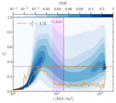
Figure 1: PDF of the sound speed squared as function of the energy density. The purple region marks the $95\%$-interval of maximum central energy densities, so that the vertical purple line represents an estimate for the largest possible energy density in a neutron star. The orange contour marks the region containing EOSs with $c^{2}_{s}<1/3$.

The orange line in Fig. 1 marks the region of the EOSs that are sub-conformal, i.e., with $c_{s}^{2}<1/3$, at all densities (the horizontal dashed line that marks $c_{s}^{2}=1/3$). Note that around $500\,{\rm MeV}/{\rm fm}^{3}$, the orange contour spans a very thin region, indicating that at these energy densities the sub-conformal EOSs have an obvious upper bound $c_{s}^{2}<1/3$, but also a less-obvious lower bound $c_{s}^{2}\gtrsim 0.2$. This is an important feature that explains why these EOSs are so difficult to produce. Indeed, as revealed by the colormap, the number of EOSs that fall in this region is very small and amounts to only $\simeq 5\times 10^{-5}$ of the total. The fraction of sub-conformal EOSs increases slightly if we restrict the range of densities to those that are admissible for neutron-star interiors, becoming $\simeq 3\times 10^{-4}$ of the total. The reason for this increase is that many of the EOSs that are sub-conformal for $e\lesssim 300\,{\rm MeV/fm^{-3}}$, tend to stiffen at larger energy densities, thus becoming super-conformal.

The colormap of the PDF in Fig. 1 also reveals the presence of a second peak at large energy densities, close to where the perturbative QCD boundary conditions are imposed and reflects artefacts of the parametrization method, which allows for large variations in the sound speed at very high energy densities, where $c_{s}^{2}$ is expected to be close to the asymptotic value $1/3$. Fortunately, the energy densities where this second peak appears are far from those expected in the interior of neutrons stars. It is also possible to reduce the extent of this second peak by imposing a criterion that filters out EOSs whose sound speeds vary strongly on small scales as done by Annala et al. (2020). However, given the very poor knowledge of the behaviour of the sound speed at these regimes, we prefer to report the unfiltered results. What matters here is that, when imposed, the filtering has no significant impact on the PDF at the energy densities that are relevant for stellar interiors (see the Appendix for a discussion).

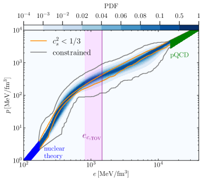
Figure 2: PDF of the pressure as function of the energy density. The blue and green regions mark the uncertainties in pressure in nuclear theory (Hebeler et al., 2013) and perturbative QCD (Fraga et al., 2014), respectively. The gray contour encloses all EOSs satisfying the astronomical constraints, while the purple regions and the orange contour are the same as in Fig. 1.

Figure 2 shows the corresponding PDF of the pressure as a function of the energy density with the same conventions as in Fig. 1. In addition, we indicate with a gray line the outer envelope of all constraint satisfying solutions, which is very similar to the one found by Annala et al. (2020). However, an important difference with respect to Annala et al. (2020), where no information on the distribution is offered, is that the PDF reveals that the large majority of EOSs accumulates in a band that is much narrower than the allowed gray region. Interestingly, at almost all energy densities, the pressure is either inside or close to the sub-conformal region, except around $e\approx 500\,{\rm MeV}/{\rm fm}^{3}$. This is an important result as it reveals that it is very hard to deduce the poor likelihood of sub-conformal EOSs when looking at the behaviour of the pressure only.

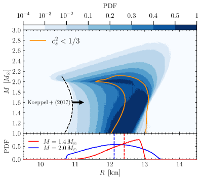
Figure 3: Top: PDF of the mass-radius relation. The orange contour encloses EOSs with sub-conformal sound speed (see Fig. 1). The dashed black line reports the lower bound for the radii as computed from considerations on the threshold mass (Koeppel et al., 2019). Bottom: PDF cuts for stars with mass $M=1.4\,M_{\odot}$ and $M=2\,M_{\odot}$; the dashed vertical lines mark the median of the distributions.

Figure 3 shows the PDF of the masses as a function of the stellar radii. The outer edges of the distribution show $M_{{}_{\rm TOV}}\lesssim 3\,M_{\odot}$ and an approximate lower limit for the minimum radius of $R\gtrsim 10.5\,{\rm km}$. This is in remarkably good agreement with the analytic lower bound $R/{\rm km}\gtrsim-0.88\,(M/M_{\odot})^{2}+2.66\,(M/M_{\odot})+8.91$ derived when using the detection of GW170817 and the estimates on the threshold mass to prompt collapse (Koeppel et al., 2019; Tootle et al., 2021). The orange line marks again the outer envelope spanned by sub-conformal EOSs, whose maximum mass is $M\approx 2.1\,M_{\odot}$, also seen by Annala et al. (2020, 2022). This behaviour confirms on rather general grounds the tension between $c_{s,\rm max}^{2}<1/3$ and the observation of stars with $M\gtrsim 2~{}M_{\odot}$, already been pointed out (see, e.g.,  Bedaque & Steiner, 2015; Alford et al., 2015; Tews et al., 2018).

In the bottom panel of Fig. 3 we report slices of the PDF for two selected masses, namely, $1.4$ and $2.0\,M_{\odot}$. The median values (dashed lines) and the $95\%$ confidence levels allow us to estimate the corresponding radii as $R_{1.4}=12.42^{+0.52}_{-0.99}\,{\rm km}$ and $R_{2.0}=12.11^{+1.11}_{-1.23}\,{\rm km}$, respectively. The significant skew in the distribution for $M=1.4\,M_{\odot}$ is due to the tidal-deformability constraint which penalizes large radii. Despite the different method, our estimate for the median of $R_{1.4}$ is in good agreement with the piecewise polytropic estimates of Most et al. (2018a) ($12.00<R_{1.4}<13.45\,{\rm km}$) and slightly larger, but well within the error bars of the estimates by Huth et al. (2022) (see also Abbott et al., 2018; Radice & Dai, 2019; Capano et al., 2020; Dietrich et al., 2020; Biswas et al., 2021, for similar estimates).

Interestingly, we find that none of our constraint-satisfying EOSs have monotonic sound speeds, as it is required by scenario i). In order to check if the scenario i) is just unlikely or indeed inconsistent with the constraints, we construct $1.5\times 10^{7}$ EOSs with monotonic sound speed, hence sampling the sound speed in $c^{2}_{s}\in[0,1/3]$, without imposing a lower bound on $M_{{}_{\rm TOV}}$. We then find that these EOSs are only able to support a maximal mass $M_{{}_{\rm TOV}}<1.99\,M_{\odot}$ and are therefore excluded by a two-solar mass bound (see the Appendix for the PDF of this constraint-violating subset).

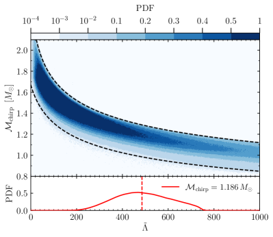
Figure 4: Top: PDF of the chirp mass as a function of the binary tidal deformability. Shown as black dashed lines are analytic fits for the minimum and maximum values of $\tilde{\Lambda}$ for a given chirp mass. Bottom: PDF cut for a binary with the same chirp mass as in GW170817, $\mathcal{M}_{\rm chirp}=1.186\,M_{\odot}$; the red dashed vertical line marks the median.

We conclude our discussion on the statistical properties of our EOSs with what arguably is one of the most important results of this work. More specifically, we report in Fig. 4 the PDF of the binary deformability shown as a function of the chirp mass. In essence, for any EOS in our sample, we randomly collect $100$ pairs of $M_{1,2},\,\Lambda_{1,2}$, out of which we compute $\mathcal{M}_{\rm chirp}$ and ${\tilde{\Lambda}}$. The results are then binned and color-coded as in the other PDFs. We find this is a particularly important figure as it relates a quantity that is directly measurable from gravitational-wave observations, $\mathcal{M}_{\rm chirp}$, with a quantity that contains precious information on the microphysics ${\tilde{\Lambda}}$. In this way, we find that the binary tidal deformability of a GW170817-like event is constrained to be $\tilde{\Lambda}_{1.186}=483^{+224}_{-210}$, at $95\%$ confidence level. The lower bound is a prediction while the upper bound effectively reflects the constraint imposed on $\tilde{\Lambda}$. Furthermore, we have fitted the $99\%$ confidence contours of the PDF with simple power-laws (dashed black lines) to obtain analytic estimates for the minimum (maximum) value of $\tilde{\Lambda}$ as function of the chirp mass

$$\tilde{\Lambda}_{\rm min\,(max)}=a+b\,\mathcal{M}_{\rm chirp}^{c}\,,$$ (7)

where $a=-50\,(-20)$, $b=500\,(1800)$, and $c=-4.5\,(-5.0)$. The relevance of expressions (7) is that, once a merging neutron-star binary is detected and its chirp mass is measured accurately, it is straightforward to use Eq. (7) to readily obtain a lower and an upper bound on the binary tidal deformability of the system. This has not been possible so far, where only upper limits have been set (Abbott et al., 2018).

Finally, to provide a graphical representation of our statistics, we show in Fig. 5 the relative weight of the various sets into which our total sample of EOSs can be decomposed, either when subject to the observational constraints (dark blue) or when not (light blue). Note that the heights of the light-blue bars in Fig. 5 for scenarios i) (fourth bar) and iii) (first bar) are not the same. In other words, the unconstrained samples of these scenarios are not equally populated. This is simply because we sample the sound speed uniformly, so that the EOSs in which all of the values of $c^{2}_{s}$ have to fall below $1/3$, as required for scenario i), are statistically suppressed when compared to the generic scenario iii), where $c^{2}_{s}$ can assume values in the full range $[0,1]$. What matters, however, is the relative difference in the constrained/unconstrained samples (see stellar markers), which is an order of magnitude smaller for scenario i) than for scenario iii). This means that iii) is statistically preferred over i) by the observational data. Furthermore, we note that in our full set we do not find any EOS with monotonic $c_{s}^{2}$ at all densities that satisfies the observational constraints.

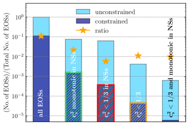
Figure 5: Schematic representation of the various sets into which our total sample of EOSs can be decomposed, either when subject to the observational constraints (dark blue) or when not (light blue). The ratio between the two samples is shown with a stellar marker, while the hatched color-coding reflects that used in Fig. 1 and in the Appendix.

4 Conclusion

We have constructed a large number of viable EOSs and studied the statistical distributions of the corresponding sound speed, mass-radius relation, and binary tidal deformability. We found that a steep rise in the sound speed and a peak $c^{2}_{s}>1/3$ is statistically preferred and that EOSs with sub-conformal sound speeds, i.e., $c^{2}_{s}\leq 1/3$, are possible within the stars, but also that they are unlikely, although in principle possible, being only $0.03\%$ of our sample. Hence, it is natural to expect that $c^{2}_{s}>1/3$ somewhere inside the neutron stars. Furthermore, imposing sub-conformality already at the level of the sampling has allowed us to resolve the range of these EOSs more accurately and identify a lower bound for the sound speed $c_{s}^{2}\gtrsim 0.2$ around $e\approx 590\,{\rm MeV}/{\rm fm}^{3}$. Interestingly, we were not able to find solutions with monotonic sound speed. Exploiting the statistical robustness of our large sample, we have obtained estimates at $95\%$ credibility of neutron-star radii for representative stars with masses of $1.4$ and $2.0$ solar masses, namely, $R_{1.4}=12.42^{+0.52}_{-0.99}\,{\rm km}$, $R_{2.0}=12.12^{+1.11}_{-1.23}\,{\rm km}$, and for the binary tidal deformability of the GW170817, $\tilde{\Lambda}_{1.186}=485^{+225}_{-211}$.

Remarkably, the very agnostic predictions on the mass-radius relations emerging from our statistics matches well the analytic predictions on the minimum stellar radius coming from very different arguments, namely the threshold mass to gravitational collapse. New radius and mass measurements, as well as gravitational-wave detections of binary neutron-star mergers will allow us to improve these estimates and narrow down our PDFs further. For example, the discovery of a neutron-star with mass larger than $2.1\,M_{\odot}$ would eliminate the possibility of sub-conformal EOSs entirely. Future work will consider improved constraints at neutron-star densities from perturbative QCD such as those recently suggested by Komoltsev & Kurkela (2022). In addition, alternative approaches to the construction of the EOSs (e.g., piecewise polytropes (Most et al., 2018b) or spectral paramaterization (Lindblom & Indik, 2012)) will help determine a potential bias introduced by our method, which is however expected to be much smaller than the observational uncertainties.

Note: After the completion of this work, a new mass measurement of $2.35\pm 0.17\,M_{\odot}$ has been published for the pulsar in the binary system PSR J0952-0607 (Romani et al., 2022). This new mass bound has no impact on the main results and conclusions presented here. While a detailed discussion is beyond the scope of this paper, the impact of very large maximum masses on the internal properties of neutron stars is instead analyzed by (Ecker & Rezzolla, 2022).

Appendix A Details about EOS construction

The material presented here is meant to provide additional information on some of the details of our calculations and on their robustness.

We start by showing in Fig. 6 some illustrative examples of our method for the construction of the EOSs. For simplicity, we concentrate on three representative examples referring to a generic EOS (i.e., an EOS with no specific behaviour of the sound speed; red solid line), a sub-conformal EOS (i.e., an EOS with $c^{2}_{s}<1/3$; blue solid line), and monotonic sound speed inside neutron stars (i.e., an EOS with monotonic $c^{2}_{s}$ for $e\lesssim e_{c,{\rm TOV}}\approx 1.3\,{\rm GeV}\,{\rm fm}^{-3}$ in this case; green solid line). More specifically, the plot on the left shows the sound speed as function of the energy density; note that the curves are continuous but with discontinuous derivatives and that the kinks in the curves mark the matching points of the various segment used to construct the EOSs. The middle panel shows the corresponding EOSs, together with the BPS EOS (Baym et al., 1971) (cyan solid line) that we use at low densities. The blue and green bands are the uncertainties from nuclear theory (Hebeler et al., 2013) and perturbative QCD (Fraga et al., 2014), respectively. We also show in gray the outer envelope of all constraint-satisfying EOSs. Finally, the right panel shows the corresponding mass-radius curves, together with the outer envelope and various observational constraints (Miller et al., 2021; Riley et al., 2021; Antoniadis et al., 2013; Cromartie et al., 2020; Fonseca et al., 2021) we impose. Note that the gray contour reproduces the hump at large radii around $M\approx 1.2\,M_{\odot}$, also seen by Annala et al. (2020), and which was associated to dynamically unstable solutions by Jiménez & Fraga (2021). Comparing this part of the contour to Fig. 3 in the main text clearly shows that the solutions in this region are possible but very unlikely.

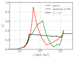
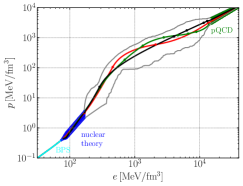
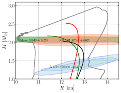
Figure 6: Representative examples referring to a generic EOS (red solid line), a sub-conformal EOS (blue solid line), and monotonic sound speed inside neutron stars (green solid line). The left plot shows the sound speed as function of the energy density, with the kinks in the curves marking the matching points of the various segment used to construct the EOSs. The middle panel shows the corresponding EOSs, together with the BPS EOS (Baym et al., 1971) (cyan solid line) that we use at low densities. The blue and green bands are the uncertainties from nuclear theory (Hebeler et al., 2013) and perturbative QCD (Fraga et al., 2014), respectively. Shown in gray is the outer envelope of all constraint-satisfying EOSs. The right panel reports the corresponding mass-radius curves, together with the outer envelope and various observational constraints.

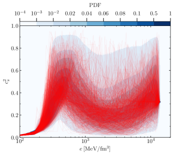
Figure 7: The same as Fig. 1 in the main text, but with the overlay of the sound-speed curves relative to 1000 different EOSs.

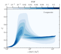
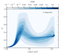
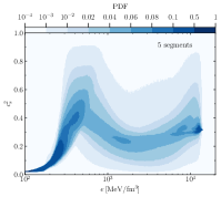
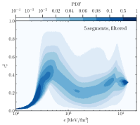
Figure 8: PDFs of the sound speed obtained for different values of the number of segments. More specifically, the first three panels from the left refer to $N=3,4,5$, respectively. They clearly show that the steep increase of the distribution beyond $c^{2}_{s}\simeq 1/3$ at small energy densities is a robust result that is independent of the number of segments and filtering. The right-most panel refers instead to a PDF for $N=5$ in which the filtering on the energy-density gradient is applied. Note how the filtering does modify the behaviour of the PDF at very large energy densities removing the most extreme EOSs.

Figure 1 of the main text shows the PDF of $c^{2}_{s}$ as a function of the energy density and a discretized colormap. Note that the steep increase to $c_{s}^{2}\gtrsim 1/3$ for $e\lesssim 500\,{\rm MeV}/{\rm fm}^{3}$, thus signalling a significant stiffening of the EOS at these densities and a subsequent decrease of the sound speed for larger energy densities. As a visual aid on how this steep increase is produced, Fig. 7 is the same as Fig. 1 in the main text, but with the overlay of the sound-speed curves relative to 1000 different EOSs.

We next consider the impact that the number of segments employed in the construction of the piece-wise linear segments for the calculation of the sound speed. As pointed out by Annala et al. (2020), constructing EOSs from piece-wise linear segments for the sound speeds can lead to rather extreme EOSs, that is, EOSs having rapidly changing material properties, especially close to where the boundary conditions are imposed. We also observe this effect in our calculation and find it to be enhanced when using a large number of segments. In principle, it is possible to introduce a criterion that discards such solutions with strongly varying sound speed. For example, Annala et al. (2020) demanded that the energy densities at two successive inflection points do not have an excessive relative variation, i.e., $(e_{i}-e_{i+1})/e_{i}>\Delta\ln e$ with $\Delta\ln e=0.5$. In this way, models with steep gradients on small energy scales are filtered out. Here however, and as mentioned in the main text, we have decided not to apply such a filter but provide evidence in this section that the first peak in the sound speed is a robust feature that is independent of the number of segments and filtering.

A sufficiently large number of segments is important to avoid a too coarse description of the sound speed and related artefacts that we discuss further below. We note that the setup just described is able to approximate phase transitions very closely. However, obtaining a “perfect” first-order phase transition requires that two consecutive draws for the sound speed are exactly zero. Since we do not explicitly demand that this happens, perfect first-order phase transitions are very unlikely in practice, but our results include a number of cases with very low sound speed at two neighboring matching points. On the one hand, choosing $N$ to be small could lead to EOSs that are rather crude and possibly suffer from intrinsic biases. On the other hand, if $N$ is very large, the whole construction can be excessively expensive from a computational point of view. Hence, an optimal choice needs to be found for $N$. In Fig. 8 we compare the PDFs for different values of the number of segments with and without filtering. Choosing a low number of segments (e.g., $N=3,4$) has the effect of influencing the distribution of the sound speed mostly at intermediate and high densities close to the perturbative QCD boundary conditions. This is shown in the first two panels on the left of Fig. 8, which refer to $N=3,4$, respectively; the third panel from the left refers instead to $N=5$ and clearly indicate that a sufficiently large number of segments is necessary to avoid artefacts at large energy densities. When comparing the PDF for $N=5$ with that obtained in Fig. 1 of the main text, where $N=7$, indicates that the latter is already a sufficiently large number of segments; indeed, experiments carried out on a limited set of EOSs with $N=9$ has shown that the differences in the PDFs are very small. Overall, the first three panels of the figure show that the steep increase of the distribution beyond $c^{2}_{s}\simeq 1/3$ at small energy densities is a robust result that is independent of the number of segments and filtering. Finally, note that the right-most panel in Fig. 8 refers to a PDF for $N=5$ in which the filtering on the energy-density gradient is applied. Note how the filtering does modify the behaviour of the PDF at very large energy densities removing the most extreme EOSs. It remains unclear whether this should be considered as more realistic PDF.

Having a different number of segments also impacts the PDFs of the pressure as a function of the energy density. This is reported in Fig. 9, which shows the outer envelope of constraint satisfying solutions for different numbers of segments and reported with various gray curves. Note that all PDFs refer to the EOSs that have not been filtered, while the light-red curve is the result for five segments and a filter on the relative energy density $\Delta\ln e=0.5$. Note that a parametrization with three segments results in a band that is significantly narrower than for larger numbers of segments. However, a comparison with Fig. 2, which was done with seven segments, suggests that most of the missed solutions fall inside the sparsely populated region. Increasing the number of segments from three to seven clearly shows that already five segments lead to a well-converged result for the outer envelope. Finally, inspecting the light-red curve it is possible to appreciate that the filtering affects mostly the regions close to the boundary conditions at low and very high energy densities, leaving the contours in between essentially unchanged.

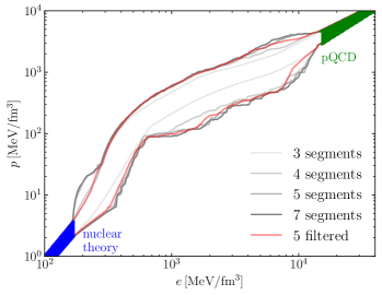
Figure 9: Outermost contours of constraint-satisfying EOSs. Gray curves are obtained from unfiltered sampling with three, four, five, and seven segments; the light red contour refers to the five-segments EOS after filtering.

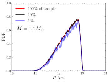
Figure 10: PDF of stellar radii at a fixed mass $M=1.4\,M_{\odot}$ for different fractions of our sample. Clearly, having a large number of EOSs decreases the size of the fluctuations; however $10\%$ of the sample is already sufficient to obtain robust estimates of the median.

We should note that the position of the peak in the sound speed at neutron-star densities is most probably related to the boundary conditions set at high densities. Ideally, it would be interesting to study how the properties of the peak in the sound speed varies when different boundary conditions in the pQCD limit are imposed. Doing so, however, is far from trivial than it might seems. The actual reason for this peak ((see also Gorda et al., 2022) is not so much the conformal value of the sound speed, but, rather, the values of the QCD pressure and the fact that they must be approached in a causal manner by our sampled EOS models. In order to relax these boundary condition one would need to define a new range for the pressure as well as a relation between the pressure and the energy density that leads to the desired value of the sound speed. This is equivalent to formulating an alternative EOS model that would differ from the established perturbative QCD result. If such a self-consistent model were available and was employed in our analysis, it would most likely move the location at which the sound speed has to decrease in order to meet the high-density boundary conditions. Unfortunately, however, this model is not presently available, at least to the best of our knowledge; hence, a purely ad-hoc change in the high-density regime may lead to physically inconsistent results.

Another aspect of our analysis that is worth discussing is the number of EOS that is necessary to use to have a statistically robust description of the PDFs. As mentioned in the main text, we have computed at total of $1.5\times 10^{7}$ EOSs and we have found that such a large number is sufficient to obtain a variance that is of $\sim 3\%$ at most. This is shown in Fig. 10, which reports a cut of the PDF for a reference mass of $M=1.4\,M_{\odot}$ when considering different fractions of our sample. In particular, the red line provides the section of the PDF when all EOSs are taken into account and corresponds therefore to the red line reported in the bottom part of Fig. 3 of the main text. Shown instead with black and blue lines are the cuts when considering only $10\%$ or $1\%$ of the sample, respectively. Note that having only $10\%$ of the EOSs in the sample is sufficient to obtain robust estimates of the median.

We conclude this Appendix with a discussion focused on the properties of the EOSs that lead to sound speeds that are monotonic. As mentioned in the main text, because these EOSs are rather rare from a statistical point of view, it is convenient to construct our ensemble by sampling the sound speed not across all of its possible values, i.e., $0\leq c^{2}_{s}\leq 1$, but only in the relevant regime, i.e., $0\leq c^{2}_{s}\leq 1/3$. In this way, it was possible to produce a separate and rich ensemble of $1.5\times 10^{6}$ EOSs with sound speed increasing monotonically and for which no observational constraints on the maximum mass were imposed.

These results are summarised in Fig. 11, whose two panels show the corresponding PDFs for the sound speed as a function of the energy density (left panel) and of the mass as a function of the stellar radius (right panel). In this respect, they can be compared with Figs. 1 and 3 of the main text, where however the green contour is now used to mark the entire span of the PDFs. Interestingly and importantly, the PDFs reveal that the largest mass that can be sustained in this case is $M\leq 1.99M_{\odot}$.

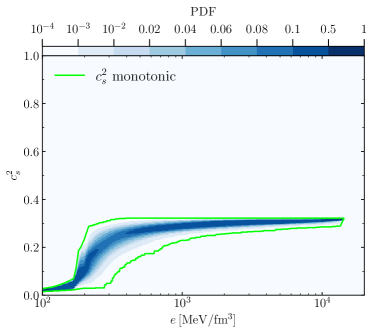
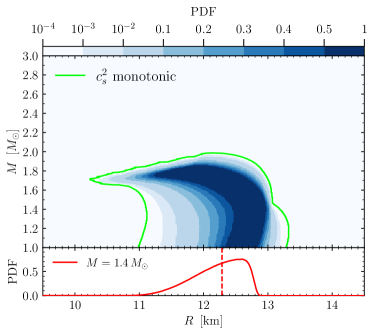
Figure 11: PDF for the sound speed (left panel) and the mass-radius relation (right right) of monotonic EOSs without observational constraints. Note that no stellar model can be found with mass $M\gtrsim 2\,M_{\odot}$.

References

- Abbott et al. (2018) Abbott, B. P., Abbott, R., Abbott, T. D., et al. 2018, Physical Review Letters, 121, 161101, doi: 10.1103/PhysRevLett.121.161101
- Alford et al. (2015) Alford, M. G., Burgio, G. F., Han, S., Taranto, G., & Zappalà, D. 2015, Phys. Rev. D, 92, 083002, doi: 10.1103/PhysRevD.92.083002
- Annala et al. (2022) Annala, E., Gorda, T., Katerini, E., et al. 2022, Physical Review X, 12, 011058, doi: 10.1103/PhysRevX.12.011058
- Annala et al. (2020) Annala, E., Gorda, T., Kurkela, A., Nättilä, J., & Vuorinen, A. 2020, Nature Physics, 16, 907, doi: 10.1038/s41567-020-0914-9
- Antoniadis et al. (2013) Antoniadis, J., Freire, P. C. C., Wex, N., et al. 2013, Science, 340, 448, doi: 10.1126/science.1233232
- Baym et al. (1971) Baym, G., Pethick, C., & Sutherland, P. 1971, Astrophys. J., 170, 299, doi: 10.1086/151216
- Bedaque & Steiner (2015) Bedaque, P., & Steiner, A. W. 2015, Physical Review Letters, 114, 031103, doi: 10.1103/PhysRevLett.114.031103
- Biswas et al. (2021) Biswas, B., Char, P., Nandi, R., & Bose, S. 2021, Phys. Rev. D, 103, 103015, doi: 10.1103/PhysRevD.103.103015
- Braun & Schallmo (2022) Braun, J., & Schallmo, B. 2022, Phys. Rev. D, 106, 076010, doi: 10.1103/PhysRevD.106.076010
- Capano et al. (2020) Capano, C. D., Tews, I., Brown, S. M., et al. 2020, Nature Astronomy, doi: 10.1038/s41550-020-1014-6
- Carignano et al. (2017) Carignano, S., Lepori, L., Mammarella, A., Mannarelli, M., & Pagliaroli, G. 2017, Eur. Phys. J. A, 53, 35, doi: 10.1140/epja/i2017-12221-x
- Cromartie et al. (2020) Cromartie, H. T., Fonseca, E., Ransom, S. M., et al. 2020, Nature Astronomy, 4, 72, doi: 10.1038/s41550-019-0880-2
- Demircik et al. (2022) Demircik, T., Ecker, C., & Järvinen, M. 2022, Phys. Rev. X, 12, 041012, doi: 10.1103/PhysRevX.12.041012
- Dietrich et al. (2020) Dietrich, T., Coughlin, M. W., Pang, P. T. H., et al. 2020, Science, 370, 1450, doi: 10.1126/science.abb4317
- Duarte et al. (2021) Duarte, D. C., Hernandez-Ortiz, S., Jeong, K. S., & McLerran, L. D. 2021, Phys. Rev. D, 104, L091901, doi: 10.1103/PhysRevD.104.L091901
- Ecker et al. (2017) Ecker, C., Hoyos, C., Jokela, N., Rodríguez Fernández, D., & Vuorinen, A. 2017, JHEP, 11, 031, doi: 10.1007/JHEP11(2017)031
- Ecker & Rezzolla (2022) Ecker, C., & Rezzolla, L. 2022. https://arxiv.org/abs/2209.08101
- Fonseca et al. (2021) Fonseca, E., Cromartie, H. T., Pennucci, T. T., et al. 2021, Astrophys. J. Lett., 915, L12, doi: 10.3847/2041-8213/ac03b8
- Fraga et al. (2014) Fraga, E. S., Kurkela, A., & Vuorinen, A. 2014, Astrophys. J. Lett., 781, L25, doi: 10.1088/2041-8205/781/2/L25
- Gandolfi et al. (2019) Gandolfi, S., Lippuner, J., Steiner, A. W., et al. 2019, Journal of Physics G Nuclear Physics, 46, 103001, doi: 10.1088/1361-6471/ab29b3
- Gorda et al. (2022) Gorda, T., Komoltsev, O., & Kurkela, A. 2022. https://arxiv.org/abs/2204.11877
- Greif et al. (2019) Greif, S. K., Raaijmakers, G., Hebeler, K., Schwenk, A., & Watts, A. L. 2019, Mon. Not. R. Astron. Soc., 485, 5363, doi: 10.1093/mnras/stz654
- Hands et al. (2006) Hands, S., Kim, S., & Skullerud, J.-I. 2006, Eur. Phys. J. C, 48, 193, doi: 10.1140/epjc/s2006-02621-8
- Hebeler et al. (2013) Hebeler, K., Lattimer, J. M., Pethick, C. J., & Schwenk, A. 2013, Astrophys. J., 773, 11, doi: 10.1088/0004-637X/773/1/11
- Hippert et al. (2021) Hippert, M., Fraga, E. S., & Noronha, J. 2021, Phys. Rev. D, 104, 034011, doi: 10.1103/PhysRevD.104.034011
- Huth et al. (2022) Huth, S., Pang, P. T. H., Tews, I., et al. 2022, Nature, 606, 276, doi: 10.1038/s41586-022-04750-w
- Jiménez & Fraga (2021) Jiménez, J. C., & Fraga, E. S. 2021, Phys. Rev. D, 104, 014002, doi: 10.1103/PhysRevD.104.014002
- Kanakis-Pegios et al. (2020) Kanakis-Pegios, A., Koliogiannis, P. S., & Moustakidis, C. C. 2020, Phys. Rev. C, 102, 055801, doi: 10.1103/PhysRevC.102.055801
- Keller et al. (2021) Keller, J., Wellenhofer, C., Hebeler, K., & Schwenk, A. 2021, Phys. Rev. C, 103, 055806, doi: 10.1103/PhysRevC.103.055806
- Koeppel et al. (2019) Koeppel, S., Bovard, L., & Rezzolla, L. 2019, Astrophys. J. Lett., 872, L16, doi: 10.3847/2041-8213/ab0210
- Komoltsev & Kurkela (2022) Komoltsev, O., & Kurkela, A. 2022, Phys. Rev. Lett., 128, 202701, doi: 10.1103/PhysRevLett.128.202701
- Kovensky et al. (2022) Kovensky, N., Poole, A., & Schmitt, A. 2022, Phys. Rev. D, 105, 034022, doi: 10.1103/PhysRevD.105.034022
- Leonhardt et al. (2020) Leonhardt, M., Pospiech, M., Schallmo, B., et al. 2020, Phys. Rev. Lett., 125, 142502, doi: 10.1103/PhysRevLett.125.142502
- Lindblom & Indik (2012) Lindblom, L., & Indik, N. M. 2012, Phys. Rev. D, 86, 084003, doi: 10.1103/PhysRevD.86.084003
- Margalit & Metzger (2017) Margalit, B., & Metzger, B. D. 2017, Astrophys. J. Lett., 850, L19, doi: 10.3847/2041-8213/aa991c
- Margueron et al. (2021) Margueron, J., Hansen, H., Proust, P., & Chanfray, G. 2021, Phys. Rev. C, 104, 055803, doi: 10.1103/PhysRevC.104.055803
- McLerran & Reddy (2019) McLerran, L., & Reddy, S. 2019, Phys. Rev. Lett., 122, 122701, doi: 10.1103/PhysRevLett.122.122701
- Miller et al. (2019) Miller, M. C., Lamb, F. K., Dittmann, A. J., et al. 2019, Astrophys. J. Lett., 887, L24, doi: 10.3847/2041-8213/ab50c5
- Miller et al. (2021) —. 2021, Astrophys. J. Lett., 918, L28, doi: 10.3847/2041-8213/ac089b
- Most et al. (2018a) Most, E. R., Nathanail, A., & Rezzolla, L. 2018a, Astrophys. J, 864, 117, doi: 10.3847/1538-4357/aad6ef
- Most et al. (2018b) Most, E. R., Weih, L. R., Rezzolla, L., & Schaffner-Bielich, J. 2018b, Phys. Rev. Lett., 120, 261103, doi: 10.1103/PhysRevLett.120.261103
- Moustakidis et al. (2017) Moustakidis, C. C., Gaitanos, T., Margaritis, C., & Lalazissis, G. A. 2017, Physical Review C, 95, 045801, doi: 10.1103/PhysRevC.95.045801
- Nathanail et al. (2021) Nathanail, A., Most, E. R., & Rezzolla, L. 2021, Astrophys. J. Lett., 908, L28, doi: 10.3847/2041-8213/abdfc6
- Pal et al. (2022) Pal, S., Kadam, G., & Bhattacharyya, A. 2022, Nucl. Phys. A, 1023, 122464, doi: 10.1016/j.nuclphysa.2022.122464
- Radice & Dai (2019) Radice, D., & Dai, L. 2019, European Physical Journal A, 55, 50, doi: 10.1140/epja/i2019-12716-4
- Rezzolla et al. (2018) Rezzolla, L., Most, E. R., & Weih, L. R. 2018, Astrophys. J. Lett., 852, L25, doi: 10.3847/2041-8213/aaa401
- Riley et al. (2019) Riley, T. E., Watts, A. L., Bogdanov, S., et al. 2019, Astrophys. J. Lett., 887, L21, doi: 10.3847/2041-8213/ab481c
- Riley et al. (2021) Riley, T. E., Watts, A. L., Ray, P. S., et al. 2021, Astrophys. J. Lett., 918, L27, doi: 10.3847/2041-8213/ac0a81
- Romani et al. (2022) Romani, R. W., Kandel, D., Filippenko, A. V., Brink, T. G., & Zheng, W. 2022, Astrophys. J. Lett., 934, L18, doi: 10.3847/2041-8213/ac8007
- Ruiz et al. (2018) Ruiz, M., Shapiro, S. L., & Tsokaros, A. 2018, Phys. Rev. D, 97, 021501, doi: 10.1103/PhysRevD.97.021501
- Shibata et al. (2019) Shibata, M., Zhou, E., Kiuchi, K., & Fujibayashi, S. 2019, Phys. Rev. D, 100, 023015, doi: 10.1103/PhysRevD.100.023015
- Tews et al. (2018) Tews, I., Carlson, J., Gandolfi, S., & Reddy, S. 2018, Astrophys. J., 860, 149, doi: 10.3847/1538-4357/aac267
- The LIGO Scientific Collaboration et al. (2019) The LIGO Scientific Collaboration, the Virgo Collaboration, Abbott, B. P., et al. 2019, Physical Review X, 9, 011001, doi: 10.1103/PhysRevX.9.011001
- Tootle et al. (2021) Tootle, S. D., Papenfort, L. J., Most, E. R., & Rezzolla, L. 2021, Astrophys. J. Lett., 922, L19, doi: 10.3847/2041-8213/ac350d