A Deep Learning Approach for Thermal Plume Prediction of Groundwater Heat Pumps

Abstract

Climate control of buildings makes up a significant portion of global energy consumption, with groundwater heat pumps providing a suitable alternative. To prevent possibly negative interactions between heat pumps throughout a city, city planners have to optimize their layouts in the future. We develop a novel data-driven approach for building small-scale surrogates for modelling the thermal plumes generated by groundwater heat pumps in the surrounding subsurface water. Building on a data set generated from 2D numerical simulations, we train a convolutional neural network for predicting steady-state subsurface temperature fields from a given subsurface velocity field. We show that compared to existing models ours can capture more complex dynamics while still being quick to compute. The resulting surrogate is thus well-suited for interactive design tools by city planners.

1 Introduction

Heating and cooling of buildings has garnered attention in recent years, especially as the world moves towards renewable sources of energy. One focus recently has been on using shallow geothermal energy through groundwater heat pumps (GWHP) (Halilovic et al., 2022). As the groundwater temperature is relatively stable year round, GWHPs are able to use this source to both heat and cool buildings. As cities move towards installing more GWHPs, assessing and optimizing their influence on the subsurface is required. Installing GWHPs without any restrictions could result in situations where negative interaction occurs (García-Gil et al., 2020; Daemi & Krol, 2019). GWHPs operate by extracting water from an extraction well, either heating or cooling this fluid, and re-injecting it back into the subsurface. The local temperature changes around the injection well, and a thermal plume develops due to the diffusion and advection of this water in the subsurface. This thermal plume can propagate downstream and interact with other GWHPs or even recirculate into its own extraction well, causing interference. This requires careful planning of the layout and operational loads of GWHPs (Beck et al., 2013). To provide an accurate assessment of the groundwater temperatures due to the usage of many heat pumps, high-fidelity subsurface flow simulations are required (Meng et al., 2019). Furthermore, to optimize the layout and usage of a large number of GWHPs on this scale requires many high-fidelity simulation runs, making large optimization scenarios infeasible.

A common solution is to use surrogate models, also known as low-fidelity models, which are computationally cheap to solve the optimization problem (Sbai, 2019; Nagoor Kani & Elsheikh, 2019; Robinson et al., 2012). To help optimize the layout of potentially thousands of GWHPs, surrogate models could be used to determine the local temperature influence that each GWHP has on the groundwater temperature. As the thermal influence of one heat pump can be computed fast and cheaply, many such evaluations can be performed to determine the influence of multiple heat pumps in a system. This can be used to provide either a semi-optimised solution, or to evaluate the influence of one heat pump on other previously installed heat pumps.

Analytical solutions provide a computationally cheap solution to predict the thermal plume (Pophillat et al., 2020), but suffer from several disadvantages. They often do not account for variations in the groundwater parameters in space, such as varying permeability field, pressure gradients and velocity fields. This results in the thermal plume extending in one direction only for the analytical solutions (Fig. 1(a)), however, the thermal plumes may actually change their direction due to heterogeneous groundwater parameters or obstructions.

In a typical application the optimization problem would consist of an area with many GWHP’s (such as in Fig. 1(b), and potentially much larger areas), with known geological parameters; spatially varying permeability field and pressure boundary conditions. The surrogate model must be able to provide the local temperature variation (thermal plume) around each individual GWHP (Fig. 2(c)), and we can determine which GWHPs might interact with each other.

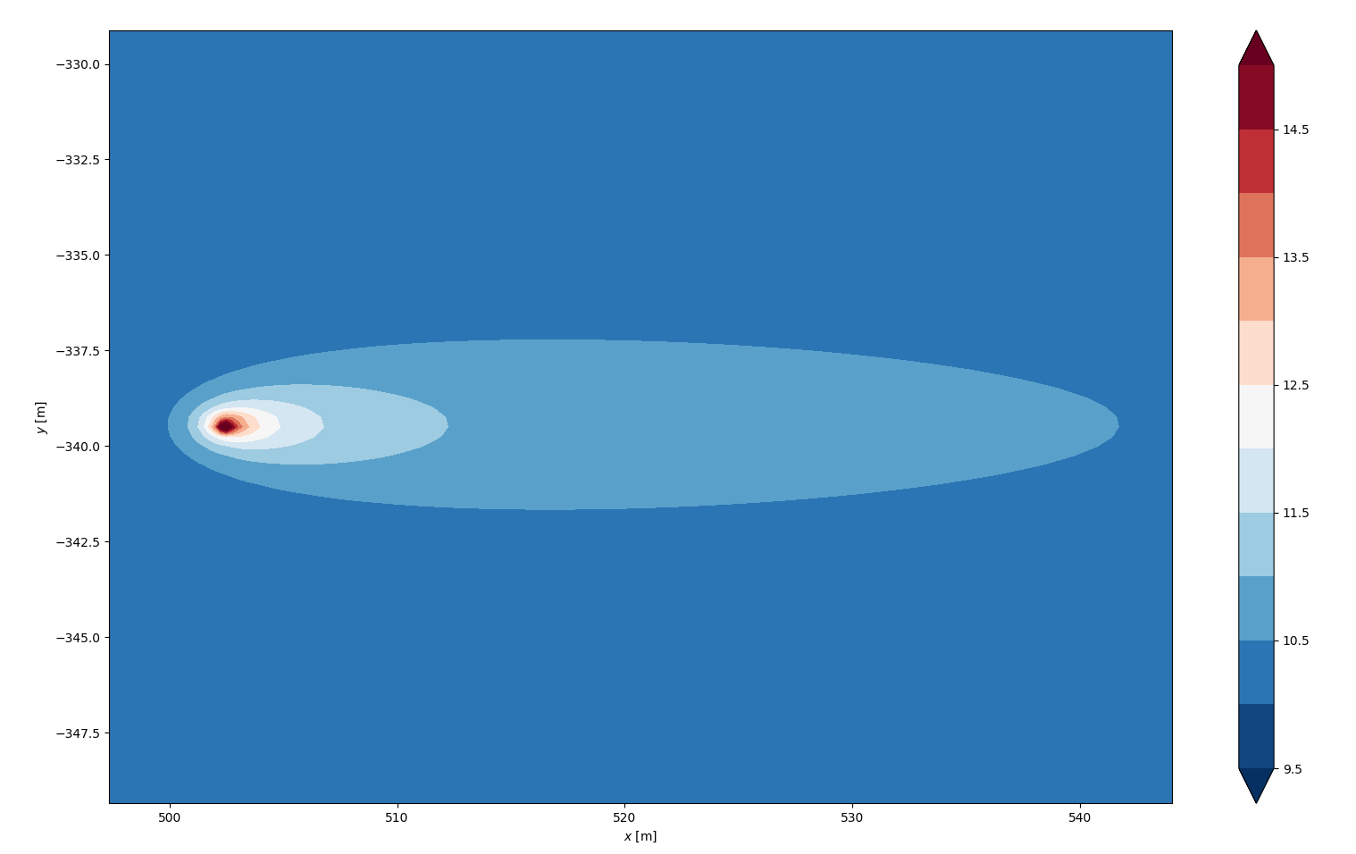
(a) Analytical thermal plume

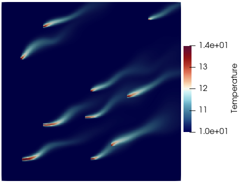
(b) Temperature field with 10 GWHPs scattered throughout the domain.

Figure 1: The thermal plume developed by (a) GWHP derived from the LAHM model (Pophillat et al., 2020) and (b) 10 GWHPs in a large domain using a spatially varying permeability field. The thermal plume in (a) is uni-directional for the analytical model, and is dependent only on the parameters at the location of re-injection. A more realistic example in (b) shows that the thermal plumes follow the velocity direction of the subsurface.

Related Work

The usage of machine learning based surrogates for physical applications has increased dramatically in recent years (Vinuesa & Brunton, 2021; Chen et al., 2021; Zhu et al., 2019). There have been purely supervised learning approaches put forth (Khoo et al., 2020) with multiple variations using e.g. convolutional neural networks (CNNs) (Tompson et al., 2017; Thuerey et al., 2019) or LSTMs (Mohan & Gaitonde, 2018) for temporal modelling. Another promising line of research are physics-informed neural networks (PINNs), where a neural network is trained to satisfy some specific boundary-value problem (Raissi et al., 2019; Tartakovsky et al., 2020; Raissi et al., 2020; Wang et al., 2020; Gao et al., 2021). Given a partial differential equation (PDE), the residual is added to the network’s loss function which is then trained to minimize this residual. Other works follow a coupled approach such as CFDNet (Obiols-Sales et al., 2020) where a neural network surrogate is used as a pre-conditioner inside a traditional numerical solver or e.g. Beck et al. (2019) where a neural network is used to model closure terms for turbulent flows. In this work, we focus on a purely supervised CNN approach for making new predictions by focusing on a very confined flow domain.

2 Method

The surrogate model only needs to solve for the local temperature field around a GWHP. We assume that the subsurface temperature is domniated by the advection term in the Darcy flow equations (Eq. 2), and the temperature profile follows the velocity field profile. Therefore, our aim is to develop a surrogate model that uses the spatially varying, steady-state groundwater velocity field as an input, and outputs the thermal plume that develops due to the addition of a single GWHP in a smaller domain.

Data Generation

In order to train the neural network, we need to provide enough training data such that the thermal plume can be accurately captured. We use PFLOTRAN (Hammond et al., 2014) to perform high-fidelity subsurface simulations. We solve for the boundary value problem using a finite volume subsurface solver to determine the pressure field, velocity field and temperature field. We consider a 2D domain with directions $x$ and $y$, and Darcy velocities ${\bm{q}}=(q_{x},q_{y})$. The training data simulations are performed on a 64x64 structured grid with 4096 cells, covering an area of 128$m$ $\times$ 128$m$ $\times$ 1$m$. The GWHP is modelled by injecting fluid of 0.05 $kg\cdot s^{-1}$ at 15 °C at the center of the domain, and run for a total of 720 days to achieve a pseudo steady-state solution. The domain temperature is set to 10 °C at time T $=$ 0.

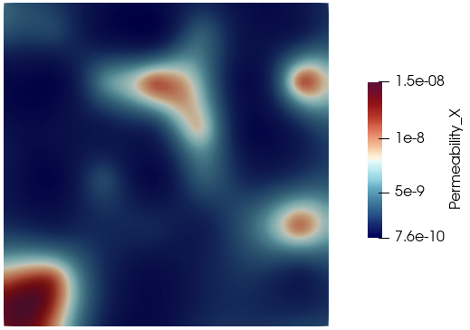
(a) Permeability Field

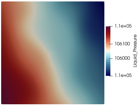
(b) Pressure Field

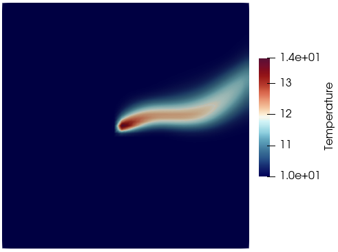
(c) Temperature Field

Figure 2: The permeability field (a), pressure field (b) and temperature field (c) for a training data example. The temperature plume that develops from the GWHP is not uni-directional like the analytical solutions, and depends on the velocity magnitude and direction.

The training data is generated by varying the permeability field and pressure boundary conditions to generate randomly varying velocity fields. The permeability field is generated by randomly assigning uniformly distributed values between $4.1\cdot 10^{-8}$ and $2.1\cdot 10^{-9}$ at various points on a $4\times 4$, $6\times 6$ and $8\times 8$ square grid throughout the domain. We use the Python library random to pseudo-randomly generate the permeability values. These values are then mapped to the PFLOTRAN grid using that radial basis function (RBF) interpolation method with global thin-plate-splines basis functions. An example permeability field is shown in Fig. 2(a).

The pressure gradient applied to the domain is also generated using the random library in Python. Two random values for the $x$ and $y$ direction of the gradient are applied. This allows us to generate many varying velocity fields, and due to the small size of the FV solver, the simulations to calculate a stead-state temperature field $T$ are computationally feasible. For more details regarding the simulation setup see Appendix B.

Preprocessing

Before using the data we apply some preprocessing to aid the training process. First, we subtract $10\degree C$ from all temperature values as this is the initial groundwater temperature we set for our simulation. We then normalize each quantity (Darcy flow $(q_{x},q_{y})$ and temperature $T$) separately by centering and scaling the data such that they are restricted to the $[-1,1]$ range. This often simplifies the learning task for NNs as has been shown previously e.g.  in (LeCun et al., 2012; Wiesler & Ney, 2011). Additionally, we augment and extend the data set by appending randomly rotated input and target images resulting in a larger data set for more robust results.

Model

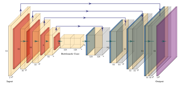
Figure 3: Visualization of the U-net type network architecture. The encoder and decoder paths feature 2D convolutions and ReLU activation functions. Both paths are connected via skip connections in each level.

For the surrogate model, we choose a slightly modified version of the “TurbNet” architecture as described in Thuerey et al. (2019) which in turn can be considered a variant of the “U-net” (Ronneberger et al., 2015). The input is given as a two-channel image with $64\times 64$ pixel values corresponding to the Darcy flow ${\bm{q}}$. The general shape is similar to a simple “U-net” where the input is convolved into coarser and coarser features on a contracting path until a bottleneck level is reached. From this on the feature channels are again de-convolved in a symmetric fashion upwards. Additionally, each step in the hierarchy also includes a skip connection, copying intermediate results from the contracting path and concatenating it feature-wise to the results of the expanding path. As output, the network produces a single channel image at the same $64\times 64$ resolution of the predicted temperature field. A graphical overview of the architecture is depicted in Fig. 3. In contrast to (Thuerey et al., 2019) we raised the feature size of the bottleneck path. Our assumption is that features which are convolved down to a single pixel value don’t hold much relevant information anymore, and we can thus save some model complexity. Additionally, we lowered the amount of channels in each block as our experiments showed good results even with fewer parameters. This approach allows us to directly predict a stationary temperature plume for any given flow field.

3 Results

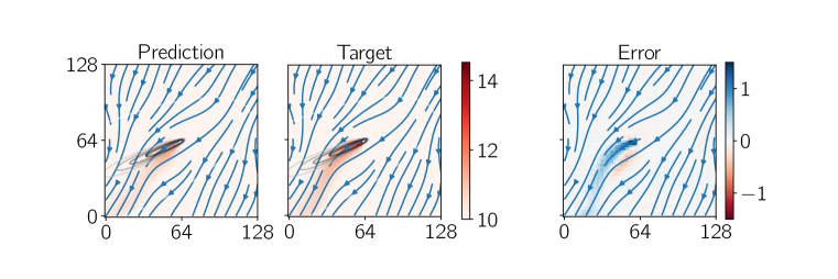
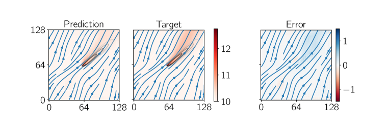
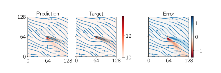
Figure 4: Prediction result and simulation ground truth for three different samples from the test data set. The predicted temperature plumes match the target in direction and shape. We show two typical results and one outlier. The rightmost column displays the error in °C. Note the different scales of the error. Analytical temperature plumes calculated with the LAHM model are overlaid on top in gray.

We trained the aforementioned model on a data set of $239$ generated samples. An additional $720$ augmented samples are created by randomly rotating the input and output images resulting in a total data set size of $959$. $192$ samples are randomly selected as validation data during training. The model is trained using the ADAM optimizer (Kingma & Ba, 2017) with a fixed learning rate $0.0004$ for $60,\!000$ epochs. For further details see Appendix A. Figure 4 shows a selection of three different predictions of the trained model which were performed using a held out test set of size $40$ which was never before seen by the model or used during training in any way. Shown in each row are the model’s prediction, the target temperature field from the numerical solution and the point-wise error between the two. Furthermore, the analytical LAHM model from Pophillat et al. (2020) is overlaid on top of both prediction and target plots. We can nicely observe that in all cases the predicted temperature plume matches the target in direction and shape. The top example prominently displays the advantage of our method when compared to the analytical model. While the analytical plume only estimates linear transport of the flow, our method provides a much more detailed prediction following the flow. The second row again is a nice example of the prediction matching the target quite well also in magnitude. Lastly, we also include an example where the model did not perform too well and deviates from the expected flow direction showing the predictions are not fully robust yet. Quantifying the error we see each example having different magnitudes ranging from $0.25$ °C to $2$ °C. Note however, that the largest error is often only encountered at the injection site with the rest of the plume showing significantly less errors. This shows it is harder to determine the initial injection temperature from the velocity magnitude at the GWHP, and deserves more attention in the future. The relative error

$$\frac{\sum_{i}\left|T^{p}_{i}-T^{t}_{i}\right|}{\sum_{i}\left|T^{t}_{i}\right|}$$

between the predicted temperatures $T^{p}$ and target temperatures $T^{t}$ achieved on the complete test data set is $0.68\%$. Considering that the analytical model plume can be offset from the real plume by $>10m$ at the end of the plume, this could make the difference in a real-world scenario when deciding whether it is feasible to place a GWHP on a specific building or not.

4 Conclusion

In this work we have demonstrated the viability of data-driven surrogate models for approximating subsurface thermal plumes generated by groundwater heat pumps. With a supervised learning approach and a suitable CNN architecture we were able to get a good agreement between fast surrogate predictions and high-fidelity ground truth data. Especially compared to simpler analytical approaches the data-driven model has shown very convincing results. This study can be seen as a first step enabling more refined approaches and applications down the line.

Considering the low inference time of the trained model ($\leq 50ms$) we could imagine it being used in close-to-real-time applications such as design tools for city planners. We would also like to expand the surrogate model by including parametric inputs such as a heat pump’s energy output. Furthermore, a shortcoming of the current approach is the limitation to a small constrained domain with only a single heat pump. To model larger scenarios with multiple heat pumps another extension could be stitching together multiple local surrogate predictions and then using these as a preconditioned starting point for solving larger numerical models on the scale of a whole city domain.

Acknowledgments

Funded by Deutsche Forschungsgemeinschaft (DFG, German Research Foundation) under Germany’s Excellence Strategy - EXC 2075 – 390740016. We acknowledge the support by the Stuttgart Center for Simulation Science (SimTech).

Appendix A Training Details

The model was implemented and trained using PyTorch (Paszke et al., 2019) on a workstation with two NVIDIA RTX 3090 GPUs. The batch size was fixed at $64$ samples and the ADAM optimizer was used with a learning rate of $4e$-$4$ and otherwise default parameters. For supervision a simple MSE loss function is employed. The model used to produce the results in Sec. 3 features a total of $480$k parameters.

Appendix B Simulation Details

The PFLOTRAN (Hammond et al., 2014) package is used to solve a steady-state thermal-hydrological problem with equations for mass and energy balance given by

$$\nabla\cdot\left(\eta{\bm{q}}\right)=\nabla\cdot\left(\eta K\nabla P\right)=Q_{w}$$ (1)

and

$$\nabla\cdot\left(\eta{\bm{q}}H\right)-\kappa\Delta T=Q_{e}$$ (2)

where $Q_{w}$ is the mass flow source term, which is non-zero only at the boundaries and at the center where mass is injected into the groundwater by the GWHP, the energy source term $Q_{e}$, enthalpy $H$, thermal conductivity $\kappa$ and temperature $T$. The relevant parameters are shown in Table 1.

Table 1: Simulation parameters

$\eta$	molar density	$55.3454010547$ $kmol/m^{3}$
$\kappa$	thermal conductivity	$0.5W/(mK)$
H	specific enthalpy of water at 10°C	$1.134945kJ/mol$

References

- Beck et al. (2019) Andrea Beck, David Flad, and Claus-Dieter Munz. Deep neural networks for data-driven LES closure models. Journal of Computational Physics, 398:108910, 2019. ISSN 0021-9991. doi: https://doi.org/10.1016/j.jcp.2019.108910.
- Beck et al. (2013) Markus Beck, Peter Bayer, Michael de Paly, Jozsef Hecht-Mendez, and Andreas Zell. Geometric arrangement and operation mode adjustment in low-enthalpy geothermal borehole fields for heating. Energy, 49:434 – 443, 2013.
- Chen et al. (2021) Wenqian Chen, Qian Wang, Jan S. Hesthaven, and Chuhua Zhang. Physics-informed machine learning for reduced-order modeling of nonlinear problems. Journal of Computational Physics, 446:110666, 2021.
- Daemi & Krol (2019) Negar Daemi and Magdalena M. Krol. Impact of building thermal load on the developed thermal plumes of a multi-borehole GSHP system in different Canadian climates. Renewable Energy, 134:550 – 557, 2019. doi: https://doi.org/10.1016/j.renene.2018.11.074.
- Gao et al. (2021) Han Gao, Luning Sun, and Jian-xun Wang. Super-resolution and denoising of fluid flow using physics-informed convolutional neural networks without high-resolution labels. Phys. Fluids, 33:073603, 2021.
- García-Gil et al. (2020) Alejandro García-Gil, Miguel Mejías Moreno, Eduardo Garrido Schneider, Miguel Ángel Marazuela, Corinna Abesser, Jesús Mateo Lázaro, and José Ángel Sánchez Navarro. Nested shallow geothermal systems. Sustainability, 12(12), 2020.
- Halilovic et al. (2022) Smajil Halilovic, Leonhard Odersky, and Thomas Hamacher. Integration of groundwater heat pumps into energy system optimization models. Energy, 238(A):121607, 2022.
- Hammond et al. (2014) Glenn E. Hammond, Peter C. Lichtner, and Richard T. Mills. Evaluating the performance of parallel subsurface simulators: An illustrative example with PFLOTRAN. Water Resources Research, 50:208–228, 2014. doi: 10.1002/2012WR013483.
- Khoo et al. (2020) Yuehaw Khoo, Jianfeng Lu, and Lexing Ying. Solving parametric PDE problems with artificial neural networks. European Journal of Applied Mathematics, pp. 1–15, 2020. doi: 10.1017/S0956792520000182.
- Kingma & Ba (2017) Diederik P. Kingma and Jimmy Ba. Adam: A method for stochastic optimization, 2017.
- LeCun et al. (2012) Yann A. LeCun, Léon Bottou, Genevieve B. Orr, and Klaus-Robert Müller. Efficient BackProp, pp. 9–48. Springer Berlin Heidelberg, Berlin, Heidelberg, 2012. ISBN 978-3-642-35289-8. doi: 10.1007/978-3-642-35289-8˙3.
- Meng et al. (2019) Boyan Meng, Thomas Vienkena, Olaf Kolditza, and Haibing Shao. Evaluating the thermal impacts and sustainability of intensive shallow geothermal utilization on a neighborhood scale: Lessons learned from a case study. Energy Conversion and Management, 199:111913, 2019.
- Mohan & Gaitonde (2018) Arvind T. Mohan and Datta V. Gaitonde. A deep learning based approach to reduced order modeling for turbulent flow control using LSTM neural networks, 2018.
- Nagoor Kani & Elsheikh (2019) J. Nagoor Kani and A.H. Elsheikh. Reduced-order modeling of subsurface multi-phase flow models using deep residual recurrent neural networks. Transport in Porous Media, 126:719 – 741, 2019.
- Obiols-Sales et al. (2020) Octavi Obiols-Sales, Abhinav Vishnu, Nicholas Malaya, and Aparna Chandramowliswharan. CFDNet: A Deep Learning-Based Accelerator for Fluid Simulations. Association for Computing Machinery, New York, NY, USA, 2020. ISBN 9781450379830. doi: https://doi.org/10.1145/3392717.3392772.
- Paszke et al. (2019) Adam Paszke, Sam Gross, Francisco Massa, Adam Lerer, James Bradbury, Gregory Chanan, Trevor Killeen, Zeming Lin, Natalia Gimelshein, Luca Antiga, Alban Desmaison, Andreas Kopf, Edward Yang, Zachary DeVito, Martin Raison, Alykhan Tejani, Sasank Chilamkurthy, Benoit Steiner, Lu Fang, Junjie Bai, and Soumith Chintala. Pytorch: An imperative style, high-performance deep learning library. In H. Wallach, H. Larochelle, A. Beygelzimer, F. d'Alché-Buc, E. Fox, and R. Garnett (eds.), Advances in Neural Information Processing Systems 32, pp. 8024–8035. Curran Associates, Inc., 2019.
- Pophillat et al. (2020) William Pophillat, Guillaume Attard, Peter Bayer, Jozsef Hecht-Méndez, and Philipp Blum. Analytical solutions for predicting thermal plumes of groundwater heat pump systems. Renewable Energy, 147:2696–2707, 2020. doi: https://doi.org/10.1016/j.renene.2018.07.148.
- Raissi et al. (2019) M. Raissi, P. Perdikaris, and G.E. Karniadakis. Physics-informed neural networks: A deep learning framework for solving forward and inverse problems involving nonlinear partial differential equations. Journal of Computational Physics, 378:686 – 707, 2019. ISSN 0021-9991. doi: https://doi.org/10.1016/j.jcp.2018.10.045.
- Raissi et al. (2020) Maziar Raissi, Alireza Yazdani, and George Em Karniadakis. Hidden fluid mechanics: Learning velocity and pressure fields from flow visualizations. Science, 367(6481):1026–1030, 2020. ISSN 0036-8075. doi: 10.1126/science.aaw4741.
- Robinson et al. (2012) T.D. Robinson, M.S. Eldred, K.E. Willcox, and R. Haimes. Surrogate-based optimization using multifidelity models with variable parameterization and corrected space mapping. AIAA JOURNAL, 46(11):2814 – 2822, 2012.
- Ronneberger et al. (2015) Olaf Ronneberger, Philipp Fischer, and Thomas Brox. U-net: Convolutional networks for biomedical image segmentation. In Medical Image Computing and Computer-Assisted Intervention – MICCAI 2015, pp. 234–241, Cham, 2015. Springer International Publishing.
- Sbai (2019) Mohammed Adil Sbai. Well rate and placement for optimal groundwater remediation design with a surrogate model. Water, 11(11), 2019.
- Tartakovsky et al. (2020) A. M. Tartakovsky, C. Ortiz Marrero, Paris Perdikaris, G. D. Tartakovsky, and D. Barajas-Solano. Physics-informed deep neural networks for learning parameters and constitutive relationships in subsurface flow problems. Water Resources Research, 56(5):e2019WR026731, 2020. doi: https://doi.org/10.1029/2019WR026731. e2019WR026731 10.1029/2019WR026731.
- Thuerey et al. (2019) Nils Thuerey, Konstantin Weißenow, Lukas Prantl, and Xiangyu Hu. Deep learning methods for Reynolds-averaged Navier–Stokes simulations of airfoil flows. American Institute of Aeronautics and Astronautics, 58(1):686 – 707, 2019. doi: https://doi.org/10.2514/1.J058291.
- Tompson et al. (2017) Jonathan Tompson, Kristofer Schlachter, Pablo Sprechmann, and Ken Perlin. Accelerating Eulerian fluid simulation with convolutional networks. In Proceedings of the 34th International Conference on Machine Learning - Volume 70, ICML’17, pp. 3424–3433. JMLR.org, 2017.
- Vinuesa & Brunton (2021) Ricardo Vinuesa and Steven L. Brunton. The potential of machine learning to enhance computational fluid dynamics. 2021.
- Wang et al. (2020) Sifan Wang, Yujun Teng, and Paris Perdikaris. Understanding and mitigating gradient pathologies in physics-informed neural networks, 2020.
- Wiesler & Ney (2011) Simon Wiesler and Hermann Ney. A convergence analysis of log-linear training. In J. Shawe-Taylor, R. Zemel, P. Bartlett, F. Pereira, and K. Q. Weinberger (eds.), Advances in Neural Information Processing Systems, volume 24. Curran Associates, Inc., 2011.
- Zhu et al. (2019) Yinhao Zhu, Nicholas Zabaras, Phaedon-Stelios Koutsourelakis, and Paris Perdikaris. Physics-constrained deep learning for high-dimensional surrogate modeling and uncertainty quantification without labeled data. Journal of Computational Physics, 394:56–81, 2019.