GraphZeppelin: Storage-Friendly Sketching for Connected Components on Dynamic Graph Streams

Abstract.

Finding the connected components of a graph is a fundamental problem with uses throughout computer science and engineering. The task of computing connected components becomes more difficult when graphs are very large, or when they are dynamic, meaning the edge set changes over time subject to a stream of edge insertions and deletions. A natural approach to computing the connected components on a large, dynamic graph stream is to buy enough RAM to store the entire graph. However, the requirement that the graph fit in RAM is prohibitive for very large graphs. Thus, there is an unmet need for systems that can process dense dynamic graphs, especially when those graphs are larger than available RAM.

We present a new high-performance streaming graph-processing system for computing the connected components of a graph. This system, which we call GraphZeppelin, uses new linear sketching data structures (CubeSketch) to solve the streaming connected components problem and as a result requires space asymptotically smaller than the space required for a lossless representation of the graph. GraphZeppelin is optimized for massive dense graphs: GraphZeppelin can process millions of edge updates (both insertions and deletions) per second, even when the underlying graph is far too large to fit in available RAM. As a result GraphZeppelin vastly increases the scale of graphs that can be processed.

1. Introduction

Finding the connected components of a graph is a fundamental problem with uses throughout computer science and engineering. A recent survey by Sahu et al. (ubiquitous, ) of industrial uses of algorithms reports that, for both practitioners and academic researchers, connected components was the most frequently performed computation from a list of 13 fundamental graph problems that includes shortest paths, triangle counting, and minimum spanning trees. It has applications in scientific computing (scientific_computing1, ; scientific_computing2, ), flow simulation (bioinformatics1, ), metagenome assembly (metagenomics1, ; metagenomics2, ), identifying protein families (protein1, ; bioinformatics2, ), analyzing cell networks (cell, ), pattern recognition (pattern1, ; pattern2, ), graph partitioning (partition1, ; partition2, ), random walks (randomwalks, ), social network community detection (lee2014social, ), graph compression (compression1, ; compression2, ), medical imaging (tumor, ), and object recognition (object, ). It is a starting point for strictly harder problems such as edge/vertex connectivity, shortest paths, and $k$-cores. It is used as a subroutine for pathfinding algorithms such as Djikstra and $A^{*}$, some minimum spanning tree algorithms, and for many approaches to clustering (clustering1, ; clustering2, ; clustering3, ; clustering4, ; clustering5, ; clustering6, ).

The task of computing connected components becomes more difficult when graphs are very large, or when they are dynamic, meaning the edge set changes over time subject to a stream of edge insertions and deletions. Applications on large graphs include metagenome assembly tasks that may include hundreds of millions of genes with complex relations (metagenomics1, ), and large-scale clustering, which is a common machine learning challenge (clustering3, ). Applications using dynamic graphs include identifying objects from a video feed rather than a static image (movingobject, ), or tracking communities in social networks that change as users add or delete friends (dynamic_social, ; dynamic_web, ). And of course graphs can be both large and dynamic. Indeed, Sahu et al.’s (ubiquitous, ) survey reports that a majority of industry respondents work with large graphs ($>1$ million nodes or $>1$ billion edges) and a majority work with graphs that change over time.

A natural approach to computing the connected components on a large, dynamic graph stream is to buy enough RAM to store the entire graph. Indeed, dynamic graph stream processing systems such as Aspen and Terrace (aspen, ; terrace, ) can efficently query the connected components of a large graph subject to a stream of edge insertions and deletions when the graph fits in RAM. However, the requirement that the graph fit in RAM is prohibitive for most large graphs: for example, a graph with ten million nodes and an average degree of 1 million, using 2B to encode an edge, would require 10TB of memory. We show in Section 6 that the Aspen and Terrace graph representations are significantly larger than this lower bound.

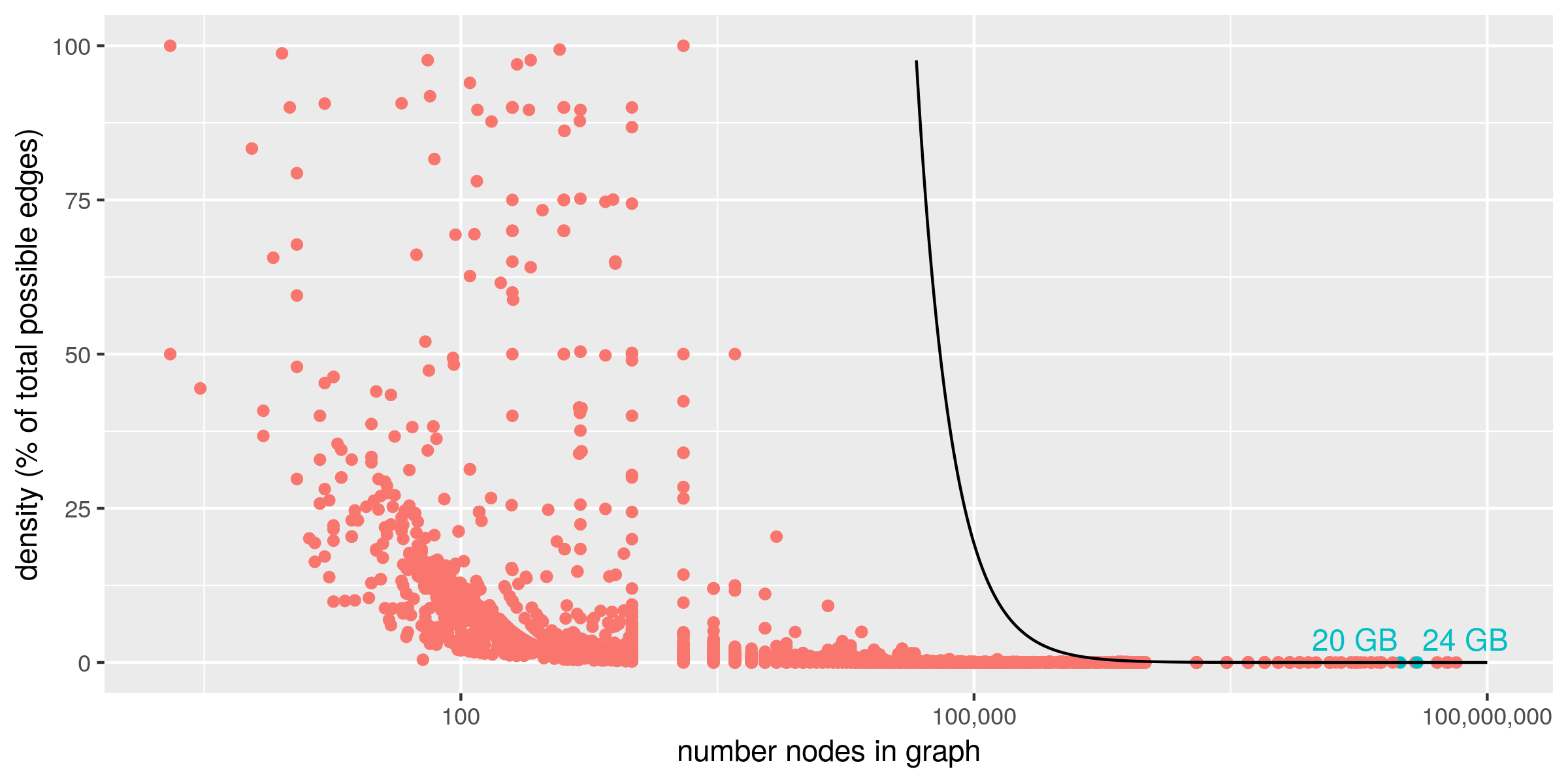
Figure 1. Published graphs have few nodes or are sparse. Each point represents a graph data set from NetworkRepository. Any point below the dark line indicates a graph that can be represented as an adjacency list in 16GB of RAM.

In public graph-data-set repositories, most graphs are smaller than typical single-machine RAM sizes. As Figure 1 illustrates, nearly all graphs in Network Repository (netrepo, ) can be stored as an adjacency list in less than 16GB. This fixed memory budget furthermore implies that graphs with large numbers of vertices must be sparse. Similarly, the Stanford SNAP graph repository and the SuiteSparse repository have few graphs larger than 16GB, and graphs with many nodes are always extremely sparse.

Large, dense graphs, we argue, are absent from graph repositories not because they are unworthy of study, but because there are few tools to analyze them. To illustrate: dense graphs do appear in Network Repository (netrepo, ), but these graphs are never larger than a few GB; moreover, as the graphs’ vertex count increases, the maximum density decreases such that the densest graphs never require more than 10 GB. A compelling explanation for the absence of large, dense graphs is selection bias: interesting dense graphs exist at all scales, but large, dense graphs are discarded as computationally infeasible and consequently are rarely published or analyzed. Moreover, some large dense graphs are known to exist as proprietary datasets: for instance, Facebook works with graphs with $40$ million nodes and $360$ billion edges. These graphs are processed at great cost on large high-performance clusters, and are consequently not released for general study.(facebookdense, )

Thus, there is an unmet need for systems that can process dense graphs, especially when those graphs are larger than available RAM. Existing systems are not designed for large, dense, dynamic graph streams and instead optimize for other use cases. Aspen and Terrace are optimized for large, sparse, dynamic graphs that completely fit in RAM, but their performance degrades significantly on dense graphs and graphs larger than RAM. There is a deep literature on parallel systems for connected components computation in multicore (greiner1994comparison, ), GPU (gpucc, ), and distributed settings (krishnamurthy1997connected, ; buvs2001parallel, ) but these focus on static graphs which fit in RAM. Many external memory (brodal2021experimental, ) and semi-external memory (abello2002functional, ) systems focus on graphs that are too large for RAM and must be stored on disk, but none of these systems focus on graphs whose edges can be deleted dynamically.

In this paper, we explore the general problem of connected components on large, dense, dynamic graphs. We introduce GraphZeppelin, which computes the connected components of graph streams using a $O(V/\log^{3}(V))$-factor less space than an explicit representation of the graph. GraphZeppelin uses a new $\ell_{0}$-sketching data structure that outperforms the state of the art on graph sketching workloads. Additionally, GraphZeppelin employs node-based buffering strategies that improve I/O efficiency. These techniques allow GraphZeppelin to scale better than existing systems in several settings. First, for in-RAM computation, GraphZeppelin’s small size means it can process larger, denser graphs than Aspen or Terrace: specifically, dense graphs twice as large as Aspen and at least 40 times larger than Terrace given 64 GB of RAM. Moreover, even if the input graph fits in RAM on all systems, GraphZeppelin is up to 2.5 times faster than Aspen and 36 times faster than Terrace on large dense graphs. Finally, GraphZeppelin scales to SSD at the cost of a 29% decrease to ingestion rate, and is more than two orders of magnitude faster than Aspen and Terrace, which suffer significant performance degradation when scaling out of RAM.

GraphZeppelin employs a new sketch algorithm, overcoming a computational bottleneck of existing linear sketching techniques in the semi-streaming graph algorithms literature (l0sketch, ). The asymptotically best existing streaming connected components algorithm is Ahn et al.’s StreamingCC (Ahn2012, ; nelson2019optimal, ), which has asymptotically low space and update time complexity. StreamingCC relies on $\ell_{0}$-sampling, which it uses to sample edges across arbitrary graph cuts. However, the best known $\ell_{0}$-sampling algorithm suffers from high constant and polylogarithmic factors in its space and update time, as we show in Section 3. This overhead makes any implementation of the StreamingCC data structure infeasibly slow and large. GraphZeppelin employs what we call CubeSketch, a specialized $\ell_{0}$-sampling algorithm for sampling edges across graph cuts, to solve the connected components problem. For large graphs CubeSketch uses 4 times less space than the best general $\ell_{0}$-sampling algorithm and can process updates more than three orders of magnitude faster.

GraphZeppelin also uses new write-optimized data structures to overcome prohibitive resource requirements of existing semi-streaming algorithms. Streaming algorithms have had a significant impact in large part because they require a small (polylogarithmic) amount of RAM. In contrast, graph semi-streaming algorithms have higher RAM requirements: for most problems on a graph with $V$ nodes, sublinear RAM is insufficient to even represent a solution so $O(V\mathrm{polylog}(V))$ RAM is typically assumed. With the large $\mathrm{polylog}$ factors, this is often more RAM than is feasible in practice; see Section 2. We propose the hybrid streaming model, which enjoys the memory advantage of the streaming model while allowing enough space in external memory to compute on dynamic graph streams. In this model there is still $O(V\mathrm{polylog}(V))$ space available, but only $O(\mathrm{polylog}(V))$ of this space is RAM and the rest is disk, which may only be accessed in $O(\mathrm{polylog}(V))$-size blocks. The simultaneous challenges in this model are to design algorithms that use small total space but also have low I/O complexity. While existing graph semi-streaming algorithms use small space, their heavy reliance on hashing and random access patterns make them slow on disk. We show that GraphZeppelin is simultaneously a space-optimal in-RAM semi-streaming algorithm and an I/O efficient external memory algorithm for the connected components problem. We also validate its performance experimentally, showing that GraphZeppelin can operate on modern consumer solid-state disk, increasing the scale of dynamic graph streams that it can process while incurring only a $29\%$ cost to stream ingestion rate.

Results.

In this paper we establish the following:

• GraphZeppelin: We present a new high-performance streaming graph-processing system for computing the connected components of a graph. This system, which we call GraphZeppelin, uses new linear sketching data structures (CubeSketch, described below) to solve the streaming connected components problem and as a result requires a $O(V/\log^{3}(V))$-factor less space than any lossless representation of the graph. GraphZeppelin is optimized for massive dense graphs: GraphZeppelin can process millions of edge updates (both insertions and deletions) per second, even when the underlying graph is far too large to fit in available RAM. As a result GraphZeppelin vastly increases the scale of graphs that can be processed.

• CubeSketch: $\ell_{0}$-sampling optimized for graph connectivity sketching. We give a new $\ell_{0}$-sampling algorithm, CubeSketch, for vectors of integers mod $2$. Given a vector of length $n$ and failure probability $\delta$, CubeSketch uses $O(\log^{2}(n)\log(1/\delta))$ bits of space and $O(\log(n)\log(1/\delta))$ average time per update, which is a factor of $O(\log(n))$ faster than the best existing $\ell_{0}$-sampler for general vectors (l0sketch, ).

  CubeSketch is a key subroutine in GraphZeppelin, where it is used to sample graph edges across arbitrary cuts as part of connected components computation. Here it is used to sketch vectors of length ${{V}\choose{2}}=O(V^{2})$, where $V$ denotes the number of nodes in the graph. We show experimentally that CubeSketch is more than 3 orders of magnitude faster than the state-of-the-art $\ell_{0}$ sampling algorithm on graph streaming workloads.

  In addition to the $O(\log(V))$-factor speedup, several non-asymptotic factors contribute to this performance improvement as well. First, the existing algorithm’s average update cost is dominated by $O(\log(V)\log(1/\delta))$ division operations, while CubeSketch’s average update cost is dominated by $O(\log(1/\delta))$ bitwise XOR operations, which are much faster. In addition, the general algorithm performs 128-bit arithmetic operations (including division) when processing graphs with more than $10^{5}$ nodes, whereas CubeSketch can use standard 64-bit operations to achieve the same error probability. Finally, both algorithms match the asymptotic space lower bound but CubeSketch uses roughly 4 times less space than the general algorithm.

• Asymptotic guarantees of GraphZeppelin: space-optimality, I/O efficiency, $O(\log^{3}(V))$ time per update. GraphZeppelin’s core algorithm matches the $O(V\log^{3}(V))$-bit space lower bound for the streaming connected components problem, and its average per-update time cost of $O(\log(V))$ is $O(\log(V)))$ times faster than the best existing algorithm (Ahn2012, ). Additionally, GraphZeppelin can efficiently ingest stream updates even when its sketch data structure is too large to fit in RAM: its I/O complexity is $sort(\text{length of stream})+O(V/B\log^{3}(V)+V\log^{*}(V))$ and for realistic block sizes it is an I/O-optimal external-memory algorithm (ChiangGoGr95, ). As a result, given a fixed amount of RAM and disk, GraphZeppelin is capable of efficiently computing the connected components of larger graphs than existing algorithms in the streaming or external memory models.

• Empirical achievements of GraphZeppelin: better scaling for in-memory, out-of-core, and parallel computation, and undetectable failure probability. GraphZeppelin’s CubeSketch-based design increases the size of input graphs that can be processed, scales well to persistent memory, and facilitates parallelism in stream ingestion. As a result, GraphZeppelin can ingest 2-5 million edge updates per second on a single scientific workstation (see Section 6), both when its data structures reside completely in RAM and also when they reside on fast disk. As a result of these advantages, GraphZeppelin is faster and more scalable than the state of the art on large, dense graphs:

  • GraphZeppelin handles larger graphs for in-RAM computation. GraphZeppelin’s space-efficient CubeSketch allows it to process graph streams larger than can be stored explicitly in a fixed amount of RAM and give it an asymptotic ${O}(V/\log^{3}(V))$ space advantage over state-of-art systems on dense graphs. Given the polylogarithmic factors and constants, we need to determine the actual crossover point where GraphZeppelin processes graphs more compactly than Aspen and Terrace. We show empirically that this crossover point occurs when the space budget is between 32 and 64 gigabytes. That is, for dense graphs on several hundred thousand nodes, GraphZeppelin is $40\%$ more compact than Aspen and several times more compact than Terrace, and this advantage only increases for larger space budgets or input sizes. Additionally, for dense graph streams on $2^{18}$ nodes GraphZeppelin ingests updates 24 times faster than Terrace and twice as fast as Aspen.

  • GraphZeppelin can use persistent memory to handle even larger graphs. GraphZeppelin’s node-based work buffering strategy facilitates out-of-core computation, allowing GraphZeppelin to use SSD to increase the scale of graph streams it can process while incurring a small cost to performance. We show experimentally that GraphZeppelin ingests updates more than two orders of magnitude faster than Aspen and Terrace when all systems swap to disk, and that using SSD slows GraphZeppelin stream ingestion by only 29%.

  • GraphZeppelin’s stream ingestion is highly parallel. GraphZeppelin employs a node-based work buffering strategy that facilitates parallelism and improves data locality. We show experimentally that GraphZeppelin’s multithreaded stream ingestion system scales well with more threads: its ingestion rate is 25 times higher with 46 threads than an optimized single-thread implementation.

  • GraphZeppelin’s theoretical failure probability is undetectable in practice. GraphZeppelin and similar graph sketching approaches achieve their remarkable space efficiency at the cost of a random chance of failure. We show empirically that GraphZeppelin’s observed failure rate is even lower than the proved (polynomially small) upper bound: in fact, for 5000 trials on real-world and synthetic graphs it never failed.

2. Preliminaries

2.1. Graph Streaming & Hybrid Graph Streaming

In the graph semi-streaming model (semistreaming1, ; semistreaming2, ) (sometimes just called the graph streaming model), an algorithm is presented with a stream $S$ of updates (each an edge insertion or deletion) where the length of the stream is $N$. Stream $S$ defines an input graph $\mathcal{G}=(\mathcal{V},\mathcal{E})$ with $V=|\mathcal{V}|$ and $E=|\mathcal{E}|$. The challenge in this model is to compute (perhaps approximately) some property of $\mathcal{G}$ given a single pass over $S$ and at most $O(V\mathrm{polylog}(V))$ words of memory. Each update has the form $((u,v),\Delta)$ where $u,v\in\mathcal{E},u\neq v$ and $\Delta\in\{-1,1\}$ where $1$ indicates an edge insertion and $-1$ indicates an edge deletion. Let $s_{i}$ denote the $i$th element of $S$, and let $S_{i}$ denote the first $i$ elements of $S$. Let $\mathcal{E}_{i}$ be the edge set defined by $S_{i}$, i.e., those edges which have been inserted and not subsequently deleted by step $i$. The stream may only insert edge $e$ at time $i$ if $e\notin\mathcal{E}_{i-1}$, and may only delete edge $e$ at time $i$ if $e\in\mathcal{E}_{i-1}$.

In Section  4 we additionally use a new variant of the graph semi-streaming model, which we call the hybrid graph streaming setting (since it incorporates some components of the external memory model (externalmemory, ) into the semi-streaming model). In this setting, there is an additional constraint on the type of memory available for computation: only $M=\Omega(\mathrm{polylog}(V))=o(V)$ RAM is available, and $D=O(V\mathrm{polylog}(V))$ disk space is available. A word in RAM is accessed at unit cost, and disk is accessed in blocks of $B=o(M)$ words at a cost of $B$ per access. Any semi-streaming algorithm can be run with this additional constraint, but may become much slower if the algorithm makes many random accesses to disk. The algorithmic challenge in the hybrid graph streaming setting is to minimize time complexity (of ingesting stream updates and returning solutions) in addition to satisfying the typical limited-space requirement of the data stream setting. In Section  4 we show how GraphZeppelin can be adapted to this model, and is both a space-optimal single pass streaming algorithm with $O(\log^{2}(V))$ update time and an I/O efficient external memory algorithm.

Problem 1 (The streaming Connected Components problem.).

Given a insert/delete edge stream of length $N$ that defines a graph $\mathcal{G}=(\mathcal{V},\mathcal{E})$, return a insert-only edge stream that defines a spanning forest of $\mathcal{G}$.

2.2. Prior Work in Streaming Connected Components

We summarize StreamingCC, Ahn et al.’s (Ahn2012, ) semi-streaming algorithm for computing a spanning forest (and therefore the connected components) of a graph.

For each node $v_{i}$ in $G$, define the characteristic vector $f_{i}$ of $v_{i}$ to be a 1-dimensional vector indexed by the set of possible edges in $\mathcal{G}$. $f_{i}[(j,k)]$ is only nonzero when $i=j$ or $i=k$ and edge $(j,k)\in\mathcal{E}$. That is, $f_{i}\in\{-1,0,1\}^{V\choose 2}$ s.t. for all $0\leq j<k<{V\choose 2}$:

$$f_{i}[(j,k)]=\left\{\begin{array}[]{ll}1&\quad i=j\text{ and }(v_{j},v_{k})\in\mathcal{E}\\ -1&\quad i=k\text{ and }(v_{j},v_{k})\in\mathcal{E}\\ 0&\quad\text{otherwise}\par\end{array}\right\}$$

Crucially, for any $S\subset\mathcal{V}$, the sum of the characteristic vectors of the nodes in $S$ is a direct encoding of the edges across the cut $(S,\mathcal{V}\setminus S$). That is, let $x=\sum_{v\in S}f_{v}$ and then $|x[(j,k)]|=1$ iff $(j,k)\in E(S,\mathcal{V}\setminus S)$.

Using these vectors, we immediately have a (very inefficient) algorithm for computing the connected components from a stream: Initialize $f_{i}=\{0\}^{V\choose 2}$ for all $i$. For each stream update $s=((u,v),\Delta)$, set $f_{u}[u,v]+=\Delta$ and $f_{v}[u,v]+=-\Delta$.

After the stream, run Boruvka’s algorithm (boruvka, ) for finding a spanning forest as follows. For the first round of the algorithm, from each $a_{i}$ arbitrarily choose one nonzero entry $(w,y)$ (an edge in $\mathcal{E}$ s.t. w = i or y = i). Add $e_{i}$ to the spanning forest. For each connected component $C$ in the spanning forest, compute the characteristic vector of $C$: $a_{C}=\sum_{v\in C}f_{v}$. Proceed similarly for the remaining rounds of Boruvka’s algorithm: in each round, choose one nonzero entry from the characteristic vector of each connected component and add the corresponding edges to the spanning forest. Sum the characteristic vectors of the component nodes of the connected components in the spanning forest, and continue until no new merges are possible. This will take at most $O(\log(V))$ rounds.

The key idea to make this a small-space algorithm is to use “$\ell_{0}$-sampling” (l0sketch, ) to run this version of Boruvka’s algorithm by compressing each characteristic vector $f_{i}$ into a data structure of size $O(\log^{2}(V))$ that can return a nonzero entry of $f_{i}$ with constant probability.

Definition 0.

A sketch algorithm is a $\delta$ $\ell_{0}$-sampler if it is

1. Sampleable: it can take as its input a stream of updates to the coordinates of a non-zero vector $a$, and output a non-zero coordinate $(j,f[j])$ of $f$. $\mathcal{S}(f)$ denotes the sketch of vector $f$.

2. Linear: for any vectors $f$ and $g$, $\mathcal{S}(f)+\mathcal{S}(g)=\mathcal{S}(f+g)$ and this operation preserves sampleability, i.e., $\mathcal{S}(f+g)$ can output a nonzero coordinate of vector $f+g$.

3. Low Failure Probability. the algorithm returns an incorrect or null answer with probability at most $\delta$.

For all $\ell_{0}$-samplers in this paper, $\mathcal{S}(f)$ is a vector and adding two sketches is equivalent to adding their vectors elementwise.

Lemma 0.

(Adapted from (l0sketch, ), Theorem 1): Given a 2-wise independent hash family $\mathcal{F}$ and an input vector of length $n$, there is an $\delta$ $\ell_{0}$-sampler using $O(\log^{2}(n)\log(1/\delta))$ bits of space.

We denote a $\ell_{0}$ sketch of a vector $x$ as $\mathcal{S}(x)$. Since the sketch is linear, $\mathcal{S}(x)+\mathcal{S}(y)=\mathcal{S}(x+y)$ for any vectors $x$ and $y$. This allows us to process stream updates as follows: we maintain a running sum of the sketches of each stream update, which is equivalent to a sketch of the vector defined by the stream. That is, let $a_{i}^{t}$ denote $a_{i}$ after stream prefix $S_{t}$. For the $j$th stream update $s_{j}=((i,x),\Delta)$ we obtain $\mathcal{S}(f_{i}^{j})=\mathcal{S}(s_{j})+\mathcal{S}(f_{i}^{j-1})$.

Linearity also allows us to emulate the merging step of Boruvka’s algorithm by summing the sketches of all nodes in each connected component. We require $O(\log(V))$ independent $\ell_{0}$ sketches for each $v\in\mathcal{V}$, one for each round, and each must succeed with probability $1-1/100$ so the size of the sketch data structure for each node is $O(\log^{3}(V))$. We refer to the sketch data structure for each node as a node sketch and each of its $O(\log(V))$ $\ell_{0}$-subsketches as CubeSketches. The total size of the entire data structure is $O(V\log^{3}(V))$. Recent work (nelson2019optimal, ) has shown that this is optimal.

The above description assumes that the exact number of nodes $V$ is known a priori. This is not strictly necessary: All we need is a loose upper bound on the number of nodes we will eventually see. Given an upper bound $U$ s.t. $V\leq U\leq V^{c}$ for some constant $c$, we can simply define $f_{i}$ to have length ${U\choose 2}$. The node sketch of $f_{i}$ then has size $O(\log^{3}(U^{2}))=O(\log^{3}(V))$. We create a node sketch for $v_{i}$ the first time it appears in a stream update $(v_{i},v_{j})$ so the total space cost is still $O(V\log^{3}(V))$. Similarly, even if nodes are identified in the input stream as arbitrary strings instead of integer IDs in the range $[V]$, we can use a hash function with range $[O(U^{2})]$ to ensure that every node gets a unique integer ID with high probability.

3. $\ell_{0}$-sampling Revisited

Existing $\ell_{0}$-sampling algorithms are asymptotically small and fast to update, but in practice high constant and logarithmic overheads in size and update time prevent these algorithms from being useful for a streaming connected components algorithm. We now review some details of the best known $\ell_{0}$-sampling algorithm and demonstrate experimentally that using it to emulate Boruvka’s algorithm for graph connectivity would be prohibitively slow and would require an enormous amount of space. Then we introduce an $\ell_{0}$-sketching algorithm which exploits the structure of the connected components problem to improve performance, and experimentally demonstrate that it is 4 times smaller and 3 orders of magnitude faster to update than the state of the art.

The best known $\ell_{0}$-sampling algorithm (l0sketch, ) is summarized in Figure 3. Given a vector $f\in\mathbb{Z}^{n}$, the data structure consists of a matrix of $\log(n)$ by $q\log(1/\delta)$ ”buckets” (for some small constant $q$). Each bucket represents the values at a random subset of positions of $f$. This representation is lossy: we can recover a nonzero element of $f$ from bucket $\mathcal{B}_{i,j}$ only when a single position in $\mathcal{B}_{i,j}$ is nonzero. Equivalently, the support of $\mathcal{B}_{i,j}$, denoted by $supp(\mathcal{B}_{i,j})$, is 1. If $supp(\mathcal{B}_{i,j})=1$, we say that $\mathcal{B}_{i,j}$ is good, and say that it is bad otherwise. With probability $1-\delta$, $\exists i,j$ s.t. $\mathcal{B}_{i,j}$ is good and therefore we can recover a nonzero value from $f$. Each bucket includes a checksum that indicates whether it is good with high probability.

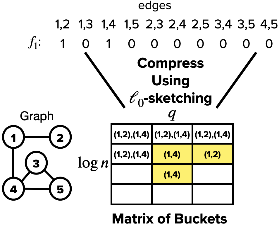
Figure 2. Compressing a characteristic vector. Each highlighted cell contains one nonzero element from the vector and can be sampled, yielding an edge incident to node 1.

Each bucket $\mathcal{B}_{i,j}$ contains three values: $a_{i,j},b_{i,j},$ and $c_{i,j}$. If $\mathcal{B}_{i,j}$ is good, then the checksum test on line 15 passes and $f[b_{i,j}]=a_{i,j}/b_{i,j}$. If the checksum test fails $\mathcal{B}_{i,j}$ is bad.

When a stream update $(e,\Delta)$ arrives, its membership in each bucket is determined using the hash function on line 3: if $hash(e)\equiv 0\pmod{2^{i}}$ then $e$ is in $\mathcal{B}_{i,j}$. If it is in bucket $\mathcal{B}_{i,j}$, it is applied to $a_{i,j},b_{i,j},$ and $c_{i,j}$ according to the logic on lines 7, 8, and 9. When the sketch is queried, it checks whether each bucket passes the checksum test on line 15. If some bucket passes this test, its sampled value is returned. Figure 2 gives an example of this process. For a more thorough analysis of this algorithm see (l0sketch, ).

1:function update_sketch(idx, $\Delta$) $\triangleright$ Add $\Delta$ to vector index ‘idx’

2:    for all col $\in[0,q\log(1/\delta))$ do

3:         col_hash $\leftarrow$ hash(col, idx)

4:         row $\leftarrow 0$

5:         checksum $\leftarrow r[\text{col}]^{\text{idx}}\mod p$

6:         while row == 0 OR col_hash[row-1] == 0 do

7:             col[row].a $\leftarrow\text{col[row].a}+\text{idx}\times\Delta$

8:             col[row].b $\leftarrow\text{col[row].b}+\Delta$

9:             col[row].c $\leftarrow\text{col[row].c}+\Delta\times\text{checksum}$

10:             row $\leftarrow\text{row}+1$              

11:function query_sketch( ) $\triangleright$ Get a non-zero vector index

12:    for all col $\in[0,q\log(1/\delta))$ do

13:         for all bucket $\in$ col do

14:             value $\leftarrow\text{bucket.a}/\text{bucket.b}$

15:             if value is integer     AND     bucket.c == $\text{bucket.b}\times r[\text{col}]^{\text{value}}\mod p$ then

16:                 return {value, bucket.b} $\triangleright$ Found a good bucket, done                           

17:    return sketch_failure $\triangleright$ All buckets bad

Figure 3. State—of—the—art $\ell_{0}$-sampling algorithm.

Existing $\ell_{0}$-samplers are slow to update for graph streaming workloads.

Note in line 9 that updating $c_{i,j}$ of bucket $\mathcal{B}_{i,j}$ requires modular exponentiation, necessitating $O(\log(n))$ multiplication operations and $O(\log(n))$ modulo operations (where the modulus is a large prime). As a result, in the worst case this algorithm performs $O(\log(n)\log(1/\delta))$ arithmetic operations per stream update. In the average case, the update modifies only $O(\log(1/\delta))$ buckets, however, the cost to generate checksums is still $O(\log(n)\log(1/\delta))$. Moreover, for sufficiently large vectors, this modular exponentiation must be done on integers larger than a 64-bit machine word, drastically increasing computation time in practice.

Vector Length	Standard $\ell_{0}$	CubeSketch	Speedup
$10^{3}$	223,000	7,322,000	33.1 x
$10^{4}$	124,000	5,180,000	42.3 x
$10^{5}$	54,800	4,384,000	79.8 x
$10^{6}$	29,300	3,730,000	127 x
$10^{7}$	20,900	3,177,000	151 x
$10^{8}$	16,300	2,825,000	172 x
$10^{9}$	13,100	2,587,000	196 x
$10^{10}$	1,350	2,272,000	1,680 x
$10^{11}$	918	2,108,000	2,300 x
$10^{12}$	833	1,963,000	2,350 x

Figure 4. CubeSketch is faster than standard $\ell_{0}$ sketching. Ingestion rates (in updates/second) are listed for both $\ell_{0}$ sketching methods.

The “Standard $\ell_{0}$” column of Figure  4 displays the single-threaded ingestion rate in updates per second of the state-of-the-art $\ell_{0}$-sampling algorithm for vectors of various sizes. These results were obtained on a Dell Precision 7820 with 24-core 2-way hyperthreaded Intel(R) Xeon(R) Gold 5220R CPU @ 2.20GHz and 64GB 4x16GB DDR4 2933MHz RDIMM ECC Memory. Note how ingestion rate decreases as vector length increases, and in particular there is a catastrophic slowdown at vector length $10^{10}$. This dramatic decrease in ingestion rate is due to the need to perform modular exponentiation on integers larger than $2^{64}$, requiring the use of 128-bit integers thus slowing computation. When sketching characteristic vectors of length $O(V^{2})$ for streaming connected components, 128-bit integers are required when $V\geq 10^{5}$.

When using $\ell_{0}$-sampling for Boruvka emulation, each stream update $((u,v),\Delta)$ must be applied to the node sketches of $u$ and $v$. For any node $u$, the node sketch of $u$ is made up of $\log(V)$ $\ell_{0}$-sketches of $a_{u}$. Each of these $\ell_{0}$-sketches has a failure rate of $\delta=1/100$ and, therefore, a width of $\log(1/\delta)=7$. Processing a stream update requires $2\cdot 7\cdot O(\log^{2}(|a_{u}|)=28\cdot O(\log^{2}(V))$ multiplication and modulo operations. For a graph with a million nodes, StreamingCC must apply each update to $28$ sketch vectors of length $10^{12}$, so it can process roughly $800/28=29$ edge updates per second.

Vector Length	Standard $\ell_{0}$	CubeSketch	Size Reduction
$10^{3}$	2.30KiB	1.21KiB	1.9 x
$10^{4}$	4.98KiB	2.34KiB	2.1 x
$10^{5}$	7.23KiB	3.43KiB	2.1 x
$10^{6}$	9.90KiB	4.73KiB	2.1 x
$10^{7}$	14.1KiB	6.79KiB	2.1 x
$10^{8}$	17.8KiB	8.58KiB	2.1 x
$10^{9}$	21.9KiB	10.6KiB	2.1 x
$10^{10}$	55.9KiB	13.6KiB	4.1 x
$10^{11}$	66.0KiB	16.1KiB	4.1 x
$10^{12}$	77.0KiB	18.8KiB	4.1 x

Figure 5. CubeSketch is significantly smaller than standard $\ell_{0}$ sketching. Sizes are listed for both $\ell_{0}$ sketching methods.

Existing $\ell_{0}$-samplers are large for graph streaming workloads.

Each node sketch consists of $\log(V)$ $\ell_{0}$ sketches and each $\ell_{0}$-sketch is a vector of $7c\log(V^{2})=14c\log(V)$ buckets. Each bucket is composed of three integers so a node sketch consists of $42c\log^{2}(V)$ integers. As noted above, 128-bit(16B) integers are necessary when $V\geq 10^{5}$, so for $c=2$ the size of a node sketch is $1344\log^{2}(V)$B. Since there is a node sketch for each node in the graph, the entire streaming data structure has size $1344V\log^{2}(V)$B. When $V=1$ million, this data structure is roughly 500 GiB in size.

Using existing $\ell_{0}$-samplers offers no advantage on modern hardware.

The goal of a streaming connected components algorithm is to use smaller space than would be required to store the entire graph explicitly. As we demonstrate empirically in Section  6, the most space-efficient dynamic graph processing system, Aspen, requires roughly 4B of space for each edge in the graph. A straightforward back-of-the-envelope calculation reveals that even for dense graphs with average degree $V/2$, StreamingCC would use less space than Aspen only on very large inputs which require enormous RAM capacities and decades of processing time: $1344V\log^{2}(V)$B $\leq 4B\cdot V^{2}/4$ only when $V\geq 5\cdot 10^{5}$. Processing a half a million-node graph using StreamingCC would require 220 GB of RAM and, at an ingestion rate of less than 35 edges per second, would take more than 56 years to process the graphs’ roughly 64 billion edges. While StreamingCC’s space complexity is much smaller than explicit graph representations like Aspen’s asymptotically, in absolute terms it offers no advantage on modern hardware.

3.1. Improved $\ell_{0}$-Sampler for Graph Connectivity

We present CubeSketch, an $\ell_{0}-$sampling algorithm for vectors on the integers mod 2, which is smaller than the best existing general-purpose $\ell_{0}$-sampling algorithm and is asymptotically faster to update. Since addition of characteristic vectors (Section 2.2) can be thought of as addition over vectors $\in\mathbb{Z}_{2}$, CubeSketch is sufficient for solving the connected components problem. Additionally, CubeSketch may be useful for other sketching algorithms for problems such as edge- or vertex-connectivity, testing bipartiteness, and finding minimum spanning trees and densest subgraphs (Ahn2012, ; GuhaMT15, ; Ahn2012_2, ; 10.1007/978-3-662-48054-0_39, ).

Since CubeSketch’s goal is to recover a nonzero entry from vectors of integers mod 2, it can use a much simpler bucket data structure than the general-purpose $\ell_{0}$-sketch, improving space and update time costs. The CubeSketch algorithm is summarized in Figure 6. Each bucket $\mathcal{B}_{i,j}$ maintains 2 values: $\alpha_{i,j}$, which is used to recover the position of a single nonzero entry, and $\gamma_{i,j}$, which is used as a checksum. $\alpha_{i,j}$ and $\gamma_{i,j}$ are each $O(\log(n))$ bits, and therefore require $O(1)$ machine words. Since each vector value is either 0 or 1, $\Delta=1$ for every stream update $(e,\Delta)$, and so for simplicity we refer to the update as $(e)$.

1:function update_sketch(idx) $\triangleright$ Toggle vector index ‘idx’

2:    for all col $\in[0,q\log(1/\delta)$ do

3:         col_hash $\leftarrow$ hash₁(col, idx)

4:         row $\leftarrow 0$

5:         checksum $\leftarrow$ hash₂(col, idx)

6:         while row == 0 OR col_hash[row-1] == 0 do

7:             col[row].$\alpha$ $\leftarrow\text{col[row].$\alpha$}\oplus\text{idx}$

8:             col[row].$\gamma$ $\leftarrow\text{col[row].$\gamma$}\oplus\text{checksum}$

9:             row $\leftarrow\text{row}+1$              

10:function query_sketch( ) $\triangleright$ Get a non-zero vector index

11:    for all col $\in[0,q\log(1/\delta))$ do

12:         for all bkt $\in$ col do

13:             if bkt.$\gamma$ == hash₂(col, bkt.$\alpha$) then

14:                 return bkt.$\alpha$ $\triangleright$ Found a good bucket, done                           

15:    return sketch_failure $\triangleright$ All buckets bad

Figure 6. Pseudocode for the CubeSketch algorithm.

Function update_sketch() in Figure 6 describes how CubeSketch processes a stream update. Given update $(e)$, if $h_{1}(e)\equiv 0\pmod{2^{i}}$ then $e$ is in $\mathcal{B}_{i,j}$. For each such $\mathcal{B}_{i,j}$, $\alpha_{i,j}=\alpha_{i,j}\oplus bin(e)$ and $\gamma_{i,j}=\gamma_{i,j}\oplus h_{2}(bin(e))$ where $\oplus$ denotes bitwise XOR, $bin(e_{w})$ denotes the binary representation of $e_{w}$, and $h_{1}$ and $h_{2}$ are hash functions drawn from a 2-wise independent family of hash functions. Note that the procedure for determining whether $e\in\mathcal{B}_{i,j}$ is identical to the algorithm in Figure 3, but the procedure for updating $\mathcal{B}_{i,j}$ is different. Importantly, CubeSketch never performs modular exponentiation, which as we will show makes it a $log(V)$ factor faster than the existing algorithm in the average case. As a result of update_sketch(), given a sequence of updates $(e_{1}),(e_{2}),\dots,(e_{k})$ to the data structure,

(1) $$\alpha_{i,j} =\bigoplus_{w\in[k]}bin(e_{w})$$

(2) $$\gamma_{i,j} =\bigoplus_{w\in[k]}h_{2}(bin(e_{w}))$$

Function query_sketch() describes how CubeSketch returns a nonzero entry of the input vector. For any bucket $\mathcal{B}_{i,j}$:

$$result=\left\{\begin{array}[]{ll}e^{\prime}&\quad\text{ if }\alpha_{i,j}=bin(e^{\prime})\>\text{ and }\>\gamma_{i,j}=h_{2}(bin(e^{\prime}))\\ \textsc{FAIL}&\quad\text{ if }\alpha_{i,j}=0\>\text{ and }\>\gamma_{i,j}=0\text{ OR}\\ &\quad\text{ if }\gamma_{i,j}\neq h_{2}(\alpha_{i,j})\end{array}\right.$$

A nonzero entry is recovered from CubeSketch by attempting to recover a nonzero entry from each $\mathcal{B}_{i,j}$ until one returns a value other than FAIL. If no such bucket exists, the algorithm returns NULL.

Theorem 1.

CubeSketch is an $\ell_{0}$ sampler that, for input vector $x\in\mathbb{Z}_{2}^{n}$, has space complexity $O(\log^{2}(n)\log(1/\delta))$, worst-case update complexity $O(\log(n)\log(1/\delta))$, average-case update complexity $O(\log(1/\delta))$, and failure probability at most $\delta$.

Proof.

The space and update time results follow by construction: each bucket $\mathcal{B}_{i,j}$ requires a constant number of machine words, and $i\in[O(\log(n)])$ and $j\in[O(\log(1/\delta)]$. Applying an update to any bucket $\mathcal{B}_{i,j}$ requires constant time, and in the worst case, an update will be applied to each of the $O(\log(n)\log(1/\delta))$ buckets. In the average case an update is applied to $O(\log(1/\delta))$ buckets.

Lemma 0.

CubeSketch’s selection process succeeds with probability at least $1-\delta$. Equivalently, CubeSketch contains a bucket $\mathcal{B}_{i,j}$ with a single nonzero entry, that is, $\Pr\left[\exists i,j\text{ s.t. }supp(\mathcal{B}_{i,j})=1\right]\geq 1-\delta.$

Proof.

Adapted from (l0sketch, ). Choose $i\in[\log(n)]$ such that $2^{i-2}\leq\lVert x\rVert_{0}<2^{i-1}$ where $\lVert x\rVert_{0}$ denotes the $\ell_{0}$ norm of $x$, i.e., the number of nonzero entries of $x$. Let $A_{x}$ be the set of positions of nonzero entries in $x$. Then, since $h_{1}$ is drawn from a 2-universal family of hash functions, $\forall j\in[6\log(1/\delta)]$,

$$\Pr\left[supp(\mathcal{B}_{i,j}=1)\right] =\sum_{k\in A_{x}}\frac{1}{2^{i}}\left(1-\frac{1}{2^{i}}\right)^{\lVert x\rVert_{0}-1}$$

$$>\frac{\lVert x\rVert_{0}}{2^{i}}\left(1-\frac{\lVert x\rVert_{0}}{2^{i}}\right)>1/8.$$

Then $\Pr\left[supp(\mathcal{B}_{i,j}\neq 1)\forall j\in[6\log(1/\delta)]\right]<(1-1/8)^{6\log(1/\delta)}=(7/8)^{6\log_{7/8}(1/\delta)/\log_{7/8}(2)}=\delta^{-6/\log_{7/8}(2)}<\delta$. ∎

Lemma 0.

CubeSketch’s checksum succeeds with high probability. That is, $\forall w,y,$ if$supp(\mathcal{B}_{w,y})=1$ then $\gamma_{w,y}=h_{2}(\alpha_{w,y})$ and if $supp(\mathcal{B}_{w,y})>1$ then $\Pr\left[\gamma_{w,y}\neq h_{2}(\alpha_{w,y})\right]\geq 1-1/n^{c}$ for some constant c.

Proof.

When $\mathcal{B}_{i,j}$ has a single nonzero entry, it always passes the error check. That is, if $supp(\mathcal{B}_{i,j})=1$, $\alpha_{w,y}=bin(e_{i})$ where $e_{i}$ is the single nonzero element of $\mathcal{B}_{i,j}$, and $\gamma_{w,y}=h_{2}(bin(e_{i}))$.

When $\mathcal{B}_{i,j}$ has more than one nonzero entry, then it passes the error check only in the rare event of a hash collision: If $supp(\mathcal{B}_{i,j})>1$, fix $e_{i}\in\mathcal{B}_{i,j}$. By equations (1) and (2), $\gamma_{w,y}=h_{2}(\alpha_{w,y})$ iff $\bigoplus_{j\in\mathcal{B}_{i,j}\setminus e_{i}}h_{2}(bin(j))\oplus h_{2}(bin(e_{i}))=h_{2}(\alpha_{w,y})$. Since $h_{2}$ is a 2-wise independent hash function, assuming that $\gamma_{i,j}$ is $c\log(n)$ bits:

$$\Pr\left[h_{2}(bin(e_{i}))=\left(\bigoplus_{j\in\mathcal{B}_{i,j}\setminus e_{i}}h_{2}(bin(j))\right)\oplus h_{2}(\alpha_{w,y})\right]=\frac{1}{2^{c\log(n)}}=\frac{1}{n^{c}}.$$

∎

Lemmas  2 and  3 imply that CubeSketch is sampleable with probability $1-\delta$ (see Definition  1). CubeSketch may be added via elementwise $\bigoplus$ (exclusive or). Linearity of CubeSketch follows from the observation that exclusive or is a linear operation. ∎

Figure  4 illustrates that CubeSketch is far faster than the standard $\ell_{0}$-sampling algorithm. In fact, when sketching characteristic vectors of graphs with at least $10^{5}$ nodes, it is more than 3 orders of magnitude faster. This dramatic speedup is a result both of CubeSketch’s asymptotically lower update time complexity, and the fact that its update cost is dominated by bitwise exclusive OR operations, which are in practice much faster than the division operations standard $\ell_{0}$-sampling performs. Finally, standard $\ell_{0}$ sampling is slowed significantly by the need to perform $O(\log(V)\log(1/\delta)$ modular exponentiation operations on 128-bit integers for each update when $V\geq 10^{5}$. CubeSketch does not require 128-bit operations until processing graphs with tens of billions of nodes.

Figure  5 shows that, for the same input vector length and failure probability, CubeSketch is twice as small as standard $\ell_{0}$ sampling for smaller vectors, and four times smaller for larger vectors. This is a result of the fact that CubeSketch’s bucket data structures use half the machine words of standard $\ell_{0}$ sampling, and the fact that CubeSketch does not need to use 128-bit integers for longer vectors.

4. Buffering for I/O efficiency and improved parallelism

In the streaming connectivity problem, stream updates are fine-grained: each update represents the insertion or deletion of a single edge. Since streams are ordered arbitrarily, even a short sequence of stream updates can be highly non-local, inducing changes throughout the graph. As a result, StreamingCC and similar graph streaming algorithms do not have good data locality in the worst case. This lack of locality can cause many CPU cache misses and therefore reduce the ingestion rate, even when sketches are stored in RAM. The cache-miss cost can be high since ingesting each stream update $(u,v,\Delta)$ requires modifying a logarithmic number of sketches, and can thus induce a poly-logarithmic number of cache misses. The consequences are even worse if sketches are stored on disk since each edge update requires loading a logarithmic number of sketches from disk, leading to the following observation.

Observation 1.

In the hybrid semi-streaming model with $M=o(V\log^{3}(V))$ RAM and $D=\Omega(V\log^{3}(V))$ disk, StreamingCC uses $\Omega(1)$ I/Os per update and processing the entire stream of length $N$ uses $\Omega(N)=\Omega(E)$ I/Os.

Any sketching algorithm that scales out of core suffers severe performance degradation unless it amortizes the per-update overhead of accessing disk. Such an amortization is not straightforward, since sketching inherently makes use of hashing and as a result induces many random accesses, which are slow on persistent storage. We now introduce a sketching algorithm for the streaming connected components problem that amortizes disk access costs, even on adversarial graph streams, and as a result is simultaneously a space-efficient graph semi-streaming algorithm and an I/O-efficient external-memory algorithm. We also note that the design facilitates parallelism, which we experimentally verify in Section 6.

4.1. I/O-Efficient Stream Ingestion

We describe GraphZeppelin’s I/O efficient stream ingestion procedure in the hybrid streaming model (see Section 2.1).

Arbitrarily partition the nodes of the graph into node groups of cardinality $\max\{1,B/\log^{3}(V)\}$. Let $\mathcal{U}\subset\mathcal{V}$ denote a node group, and let $\mathcal{S}(\mathcal{U})$ denote the node sketches associated with the nodes in $\mathcal{U}$. Store $\mathcal{S}(\mathcal{U})$ contiguously on disk. This allows $\mathcal{S}(\mathcal{U})$ to be read into memory I/O efficiently: if node groups are of cardinality 1, then $B$ is smaller than the size of a node sketch, and if each node group has cardinality $B/\log^{3}(V)>1$, then the sketches for the group have total size $O(B)$.

Applying stream update $((u,v),\Delta)$ to node sketches of $u$ and $v$ immediately upon arrival takes $\Omega(1)$ I/Os since the corresponding sketches must be read from disk. To amortize the cost of fetching sketches, GraphZeppelin only fetches $\mathcal{S}(\mathcal{U}_{i})$ when it has collected $\max\{B,\log^{3}(V)\}$ updates for $\mathcal{U}_{i}$. Since there may be $O(V)$ node groups, collecting these updates for each node group cannot be done in RAM. Instead, we collect these updates I/O efficiently on disk using a gutter tree, a simplified version of a buffer tree (Arge95thebuffer, ) which uses $O(V(\log^{3}(V))$ space.

Like a buffer tree, a gutter tree consists of a tree whose vertices each have buffers of size $O(M)$. Each non-leaf vertex has $O(M/B)$ children. We refer to a leaf vertex of the gutter tree as a gutter, because it fills with stream data but is periodically emptied by applying the contained stream data to sketches. Each leaf vertex in the gutter tree is associated with a node group $\mathcal{U}$ and has size $\max\{B,\log^{3}(V)\}$, the same size as $\mathcal{S}(\mathcal{U})$. When a gutter for node group $\mathcal{U}$ fills, GraphZeppelin reads $\mathcal{S}(\mathcal{U})$ and the updates stored in the gutter into memory, applies the updates to $\mathcal{S}(\mathcal{U})$, and writes $\mathcal{S}(\mathcal{U})$ back to disk. Since data does not persist in leaf vertices, no rebalancing is necessary.

Lemma 0.

GraphZeppelin’s stream ingestion uses $O(V\log^{3}(V))$ space and $sort(N)=O(N/B(\log_{M/B}(V/B)))$ I/Os in the hybrid streaming setting.

Proof.

GraphZeppelin’s sketch data structures use $O(V\log^{3}(V))$ space.

Each leaf in the gutter tree has a gutter of size $\max\{B,\log^{3}(V)\}$. This is one gutter for each node group and there are $V/(\max\{1,B/\log^{3}(V)\})$ node groups so the total space for the leaves of the gutter tree is $O(V\log^{3}(V))$.

In the level above the leaves, there are $V\log^{3}(V)/B\cdot B/M$ vertices each with size $M$, so the total space used at this level is $O(V\log^{3}(V))$. Each subsequent higher level of the tree uses $O(M/B)$ space less than the level below it, so the total space used for the entire gutter tree is $O(V\log^{3}(V))$.

The I/O complexity of the gutter tree is equivalent to that of the buffer tree, except that leaf gutters are flushed by reading in the appropriate sketches from disk and applying the updates in the gutter to these sketches. Asymptotically this incurs no additional cost so the total I/O complexity for ingestion is $sort(N)$. ∎

4.2. I/O-Efficient Connectivity Computation

Lemma 0.

Once all stream updates have been processed, GraphZeppelin computes connected components using $O((V\log^{3}(V)/B)+(V\log^{*}(V))$ I/Os in the hybrid streaming model.

Proof.

Each round of Boruvka’s algorithm has three phases. In the first, an edge is recovered from the sketch of each current connected component. In the second, for each edge its endpoints are merged in a disjoint set union data structure which keeps track of the current connected components. In the third phase, for each pair of connected components merged in phase 2, the corresponding sketches are summed together. We analyze the I/O cost of each phase of a round separately.

In the first round, to query the sketches in the first phase, all of the sketches must be read into RAM which can be done with a single scan. This uses $O(V\log^{3}(V)/B)$ I/Os.

The disjoint set union data structure has size $\O(V)$ and must be stored on disk. In the second phase the cost of each DSU merge is $\log^{*}(V)$ I/Os, so the total I/O cost is $V\log^{*}(V)$.

In the third phase, summing the sketches of the merged components together is I/O efficient if $B=O(\log^{3}(V))$, since the disk reads and writes necessary for summing sketches are the size of a block or larger. The cost for the third phase is $\O(V\log^{3}(V)/B)$.

If $B=\omega(\log^{3}(V))$, sketches are much smaller than the block size. Since the merges performed in each round of Boruvka are a function both of the input stream and of the randomness of the sketches, these merges induce random accesses to the sketches on disk and so summing the sketches for each merge takes $O(1)$ I/Os. In total, the third phase takes $O(V)$ I/Os in this case. ∎

Corollary 0.

When $E=\Omega(V\log^{3}(V))$ and $B=o(\log^{3}(V))$ or $M=O(V)$, GraphZeppelin is I/O optimal for the connected components problem; i.e., it uses $sort(E)=O(E/B(\log_{M/B}(V/B)))$ I/Os.

Note that for optimality the graph cannot be too sparse. In practice, for some graph streams $M=O(VB)$ and $D=O(V\log^{3}(V))$. In this case, we can omit the upper levels of the gutter tree and write I/O efficiently to the leaf gutters stored on disk. In Section  5 we describe how GraphZeppelin can perform stream ingestion using either a full gutter tree or just the leaf gutters, and evaluate the performance of both approaches in Section  6.

5. System Description

Figure 7. GraphZeppelin stream ingestion data flow.

The GraphZeppelin algorithm is split into two components: stream ingestion, in which edge updates are processed and stored using CubeSketch, and query-processing, in which a spanning forest for the graph is recovered from these sketches. These components use SSD when the sketches are so large that they do not fit in RAM. Their implementations are parallel for better performance on multi-core systems.

1:function edge_update(edge $\leftarrow$ {u, v}) $\triangleright$ Write edge update to buffers

2:    buffer_insert({u, v})

3:    buffer_insert({v, u})

4:function do_batch_update( ) $\triangleright$ Apply batched updates to supernode

5:    {batch, node} $\leftarrow$ get_batch( )

6:    for all sketch $\in$ supernodes[node] do

7:         update_sketch_batch(sketch, batch)     

8:function update_sketch_batch(sketch, batch)

9:    for all update $\in$ batch do

10:         sketch.update_sketch(update)     

Figure 8. Pseudocode for GraphZeppelin’s core stream ingestion routines. edge_update() is part of the user API, while do_batch_update(), and update_sketch_batch() are internal functions.

1:function list_spanning_forest( ) $\triangleright$ Get the connected components

2:    cleanup( ) $\triangleright$ Ensure all updates are applied

3:    found_edge $\leftarrow$ true

4:    cc_round $\leftarrow 0$

5:    spanning_forest $\leftarrow\{\}$

6:    while found_edge do $\triangleright$ loop until merging stops

7:         found_edge $\leftarrow$ false

8:         if cc_round $\geq\log_{2/3}(\text{num\_nodes})$ then

9:             return algorithm_fails $\triangleright$ Asymptotically small probability          

10:         for all supernode $\in$ supernodes do

11:             edge $\leftarrow$ supernode[cc_round].query_sketch( )

12:             if edge $\not\eq\emptyset$ then $\triangleright$ Check if cut empty, if not merge

13:                 found_edge $\leftarrow$ true

14:                 supernodes[edge.src].merge(supernodes[edge.dst])

15:                 spanning_forest.append(edge)                       

16:         cc_round $\leftarrow\text{cc\_round}+1$     

17:    return spanning_forest

18:function cleanup( )

19:    force_flush( ) $\triangleright$ Force updates out of buffers

20:    while buffers not empty do

21:         do_batch_update( )     

Figure 9. Pseudocode for GraphZeppelin’s core post-processing routines. list_spanning_forest() is part of the user API, while cleanup() is an internal function.

GraphZeppelin’s user-facing API consists of edge_update() for processing stream updates, and list_spanning_forest() to compute and return the connected components. On initialization GraphZeppelin allocates $\log(V)$ CubeSketch data structures for each node in the graph, for a total sketch size of approximately $280V\cdot\log^{2}(V)$ bytes. It also initializes its buffering data structure.

5.1. Stream Ingestion

Each update in the input stream is immediately placed into a buffering system. Periodically, the buffering system produces a batch of updates bound for the same graph node $u$. This batch is inserted into a work queue, which then hands the batch off to a Graph Worker, i.e., a thread for carrying out batched sketch updating. Because each batch is only applied to a single node sketch, and because each of the $\log(V)$ CubeSketches in a node sketch can be updated in parallel, many Graph Workers can operate in parallel without contention (see Section 5.1). A high-level illustration and pseudo code of GraphZeppelin stream ingestion are shown in Figure 7 and Figure 8 respectively.

Buffering.

GraphZeppelin’s buffering system ingests updates from the stream and periodically outputs a batch of updates for a single node in the graph. GraphZeppelin implements two buffering data structures: a gutter tree, described in Section 4, and a simplified version of the gutter tree, which only includes the leaves. Depending upon available memory, GraphZeppelin uses only one of these two buffering structures at any time. The leaf-only version is fundamentally a special case gutter tree used when sufficient memory is available $(M>V\cdot B)$ and is optimized for this case.

These buffering techniques confer several benefits. First, when GraphZeppelin’s sketches are so large that they do not fit in RAM and are stored on SSD, applying updates to a single node sketch in large batches amortizes the I/O cost of reading the node sketch into memory. Without buffering, each stream update would incur $\Omega(1)$ I/Os in the worst case. We demonstrate in Section  6.4 that buffering facilitates I/O efficiency and parallelism.

Gutter tree.

GraphZeppelin allocates $8\textsc{MB}$ for each non-leaf buffer in the gutter tree. The gutter tree writes updates to the disk in blocks of $16\textsc{KB}$, and has a fan-out of $\frac{8\textsc{MB}}{16\textsc{KB}}=512$. A write block of $16\textsc{KB}$ is an efficient I/O granularity for SSDs and a buffer size of $8\textsc{MB}$ balances buffering performance with the latency of flushing updates through the gutter tree. When $V>5\cdot 10^{4}$, the size of a sketch is greater than $100\textsc{KB}$, much larger than the $16\textsc{KB}$ block. Therefore, the leaf nodes of the gutter tree accumulate updates for a single graph node. GraphZeppelin allocates space for each leaf gutter equal to twice the size of a node sketch.

When we initialize GraphZeppelin, we leverage the static structure of the gutter tree to pre-allocate its disk space. A call to buffer_insert($\{u,v\}$) inserts $\{u,v\}$ to the root buffer of the gutter tree. Another thread asynchronously flushes the contents of full buffers to the appropriate child using the pwrite system call. When a flush causes the buffer of a child node to fill, that child node is recursively flushed before the flush of the parent continues. When a leaf gutter is full this thread moves the batch of updates into the work queue for processing by Graph Workers in do_batch_update().

Leaf-only gutter tree.

For each graph node $u$ we maintain a gutter that accumulates updates for $u$. When the system is initialized, we allocate the memory for each of these gutters. By default, each leaf gutter is 1/2 the size of a node sketch. This choice balances RAM usage with I/O efficiency as shown in Section 6.4.

buffer_insert($(u,v)$) inserts edge $e=(u,v)$ directly into the gutter for node $u$. As before, when the gutter becomes full, it is flushed and the batch is inserted into the work queue.

Note that the leaf-only gutter data structure need not fit entirely in RAM, so long as at least a page of memory is available per buffer the rest can be efficiently swapped to SSD; see Section 6.

Work queue.

The work queue functions as a simple solution for the producer-consumer problem, in which the thread filling buffers produces work and the Graph Workers consume it. Once a buffer is filled the buffer_insert() function inserts the batch of updates into the work queue. Later a Graph Worker removes the batch from the front of the queue in do_batch_update().

Insertions to the queue are blocked while the queue is full, and Graph Workers in need of work are blocked while the queue is empty. The work queue can hold up to $8g$ batches, where $g$ is the number of Graph Workers. A moderate work queue capacity of $8g$ limits the time either the buffering system or graph workers spend waiting on the queue, even when batch creation is volatile, while keeping the memory usage of the work queue low.

Sketch updates

. In each call to do_batch_update(), Graph Workers call get_batch() to receive a batch of updates bound for a particular node $u$ from the work queue. The Graph Worker then uses update_sketch_batch(sketch_u, batch) to update each of the $O(\log(V))$ CubeSketches in the node sketch of $u$.

As described in Section 3.1, a CubeSketch is a vector of buckets, each of which consists of a 64 bit $\alpha$ value and a 32 bit $\gamma$ value. Each CubeSketch stores a two dimensional array $A$ of buckets $\mathcal{B}_{i,j}$, with dimensions $\log(V^{2})\times(\log(1/\delta)=7)$. To apply an update $(e=\{u,v\})$ to a CubeSketch, the Graph Worker determines which buckets $\mathcal{B}_{i,j}$ contain $e$, and sets $\alpha_{i,j}:=\alpha_{i,j}\oplus e$ and $\gamma_{i,j}:=\gamma_{i,j}\oplus h_{y}(e)$. The hash values are calculated using xxHash (xxhash, ).

Each CubeSketch data structure uses $7\log(V^{2})=14\log(V)$ 12B buckets. In total, this is $168\log(V)$ bytes per CubeSketch, and $168\log(V)\log_{2/3}(V)$ bytes per node sketch.

Multithreading sketch updates

. Applying a batch to a node sketch in do_batch_update() is handled asynchronously by a Graph Worker, allowing what we call batch-level parallelism. We implement these workers using C++ STL threads.

We use OpenMP (ompAPI, ) to dispatch a group of threads to process each CubeSketch update in update_sketch_batch(). We refer to this as sketch-level parallelism. OpenMP allows us to specify the number of threads to allocate to a task and handles work allocation transparently. When updating a node sketch, applying a batch to each CubeSketch is treated as one work unit and OpenMP allocates the $\log(V)$ units between the apportioned threads.

Implementing both batch- and sketch-level parallelism gives us a natural way to tune GraphZeppelin’s performance. For instance, we can decide to configure more Graph Workers with fewer threads per group, or fewer Graph Workers with more threads per group. We experimentally determine a good configuration for our hardware and datasets (see Section 6.4).

A single work unit is never shared between threads in the same group. As a result, a CubeSketch is only modified by one thread in a group, so no locking is necessary at the sketch level. However, locking is necessary at the batch level because consecutive batch updates may be requested to the same node sketch, and thus multiple graph workers may seek to dispatch thread groups to the same sub-sketches. We minimize the size of this critical section by exploiting linearity of $\ell_{0}$-samplers. Rather than locking a node sketch $S(x)$ for the entire batch operation, we apply the updates to an empty sketch $S(x_{0})$ and lock only to add $S(x)=S(x)+S(x_{0})$.

5.2. Query Processing

When a connectivity query is issued, GraphZeppelin calls list_spanning_forest() which returns a spanning forest of the graph. The first step of post-processing is to flush the buffering data structure of any remaining updates, moving the batches to the work queue in cleanup(). We then wait for the Graph Workers to finish processing these batches. Finally, GraphZeppelin runs Boruvka’s algorithm to generate a spanning forest of the input graph.

6. Evaluation

Experimental setup.

We implemented GraphZeppelin as a C++14 executable compiled with g++ version 9.3 for Ubuntu. All experiments were run on a Dell Precision 7820 with 24-core 2-way hyperthreaded Intel(R) Xeon(R) Gold 5220R CPU @ 2.20GHz, 64GB 4x16GB DDR4 2933MHz RDIMM ECC Memory and two 1 TB Samsung 870 EVO SSDs. In some of our experiments we artificially limited RAM to force systems to page to disk using Linux Control Groups. We put a swap partition and the gutter tree data on one of the two SSDs, and the other SSD held the datasets.

6.1. Datasets

We used two types of data sets in this paper. First, we generated large, dense graphs using a Graph500 specification, and converted these to streams for our evaluation. We also evaluated correctness on graphs from the SNAP graph repository (snapnets, ) and the Network Repository (netrepo, ). All data sets used are described in Table 10.

Synthesizing Dense Graphs and Streams

We created undirected graphs using the Graph500 Kronecker generator. We produced five simple, undirected graphs. These graphs are dense: each has roughly one half of all possible edges. The Graph500 generator does not output simple graphs by default, so to produce our five simple graphs we pruned duplicate edges and self-loops (Ang2010IntroducingTG, ).

Name	# of Nodes	# of Edges	# Stream Updates
kron13	$2^{13}$	$1.7\times 10^{7}$	$1.8\times 10^{7}$
kron15	$2^{15}$	$2.7\times 10^{8}$	$2.8\times 10^{8}$
kron16	$2^{16}$	$1.1\times 10^{9}$	$1.1\times 10^{9}$
kron17	$2^{17}$	$4.3\times 10^{9}$	$4.5\times 10^{9}$
kron18	$2^{18}$	$1.7\times 10^{10}$	$1.8\times 10^{10}$
p2p-gnutella	$6.3\times 10^{4}$	$1.5\times 10^{5}$	$2.9\times 10^{5}$
rec-amazon	$9.2\times 10^{4}$	$1.3\times 10^{5}$	$2.5\times 10^{5}$
google-plus	$1.1\times 10^{5}$	$1.4\times 10^{7}$	$2.7\times 10^{7}$
web-uk	$1.3\times 10^{5}$	$1.2\times 10^{7}$	$2.3\times 10^{7}$

Figure 10. Dimensions of datasets used in this evaluation.

We then transformed each of the 5 graphs into a random stream of edge insertions and deletions with the following guarantees: (i) an insertion of edge $e$ always occurs before a deletion of $e$, (ii) an edge never receives two consecutive updates of the same type, (iii) we disconnect a small (fewer than 150) set of nodes from the rest of the graph, and (iv) by the end of the stream, exactly the input graph (with the exception of the edges removed to disconnect the vertices in (iii)) remains. Note that this mechanism deliberately adds edges not in the original graph, but they are always subsequently deleted. We implemented (iii) to guarantee some non-trivial connected components in each stream’s final graph.

Publicly Available Datasets

We also used the following real-world data sets. p2p-gnutella is a graph representing the Gnutella peer-to-peer network (ripeanu2002mapping, ). rec-amazon is a co-purchase recommendation graph for products listed on Amazon (leskovec2007dynamics, ), where each node represents a product and there is an edge between two nodes if their corresponding products are frequently purchased together. google-plus is a graph among users of the Google Plus social network (mcauley2012learning, ) where edges represent follower relations. web-uk is a web graph, where edges represent links between pages (netrepo, ). Each of these real-world graphs was converted to a stream using the process described above.

6.2. GraphZeppelin is Fast and Compact

We now demonstrate that, given the same memory resources, GraphZeppelin can handle larger inputs than Aspen and Terrace on sufficiently large and dense graph streams. We also show that unlike these systems, GraphZeppelin maintains good performance when its data structures are stored on SSD.

Both Aspen and Terrace are optimized for the batch-parallel model of dynamic graph processing. In this model, updates are applied to a non-empty graph in batches containing exclusively insertions or exclusively deletions. This contrasts with our streaming model, an initially empty graph is defined entirely from a stream of interspersed inserts and deletes. To avoid unfairly penalizing Aspen and Terrace, we group the input stream into batches insertions and deletions to these systems (ignoring any query correctness issues this may introduce) and present these batches as the input stream. Whenever one of these arrays fills, we feed it into the appropriate batch update function provided by Aspen or Terrace.

We ran GraphZeppelin, Aspen, and Terrace on each Kronecker stream. We used a batch size of $10^{6}$ for Aspen and Terrace because we found this to produce the highest ingestion rates for both systems. To record memory usage we logged the output of the Linux top command tracking each system every five seconds. All experiments were run for a maximum of 24 hours.

Memory profiling.

GraphZeppelin’s space-efficient CubeSketches make it a ${O}(V/\log^{3}(V))$-factor smaller than Aspen or Terrace asymptotically. Given the polylogarithmic factors and constants, this experiment determines the actual crossover point where GraphZeppelin is more compact than Aspen and Terrace. As shown in Figure 11, GraphZeppelin is smaller than Terrace even on kron15, and smaller than Aspen on kron17 and kron18.

Dataset	Aspen	Terrace	GraphZeppelin
kron13	$0.000328$	$0.000519$	$0.58$
kron15	$3.40$	$6.30$	$3.10$
kron16	$6.40$	$23.7$	$7.00$
kron17	$16.8$	$96.0$*	$15.7$
kron18	$57.7$	N/A	$35.1$

(a) Space used by each system. All numbers listed in GiB. Terrace did not finish processing kron17 within 24 hours.

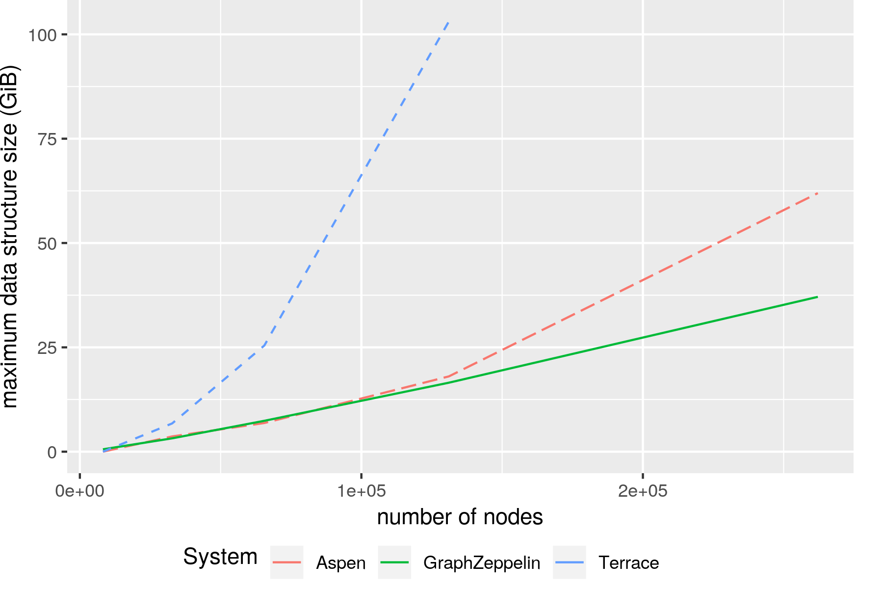
(b) GraphZeppelin is asymptotically more memory efficient than either Aspen or Terrace on large, dense graphs.

Figure 11. GraphZeppelin uses less space than Aspen or Terrace to process large, dense graph streams.

I/O Performance and Ingestion Rate.

Unlike Aspen and Terrace, GraphZeppelin maintains consistently high ingestion rates when its data structures are stored on SSD. In Figure 12(b) we summarize the results of running Aspen, Terrace, and GraphZeppelin with only 16GB of RAM. The ingestion rates of both Aspen and Terrace plummet once their data structures exceed 16GB in size and they are forced to store excess data on SSD. Neither Aspen nor Terrace were able to finish their largest evaluated stream within 24 hours ($2^{17}$ for Terrace and $2^{18}$ for Aspen). In comparison, GraphZeppelin’s ingestion rate remains high when its memory consumption extends into secondary storage. GraphZeppelin’s gutter tree finished the kron18 stream with an average ingestion rate of 2.50 million updates per second, a 29% reduction to its performance compared to when its sketches are stored entirely in RAM.

Dataset	Aspen	Terrace	Gutter Tree GZ	Leaf-Only GZ
kron13	$4.98$	$0.138$	$3.93$	$5.22$
kron15	$3.54$	$0.133$	$3.77$	$4.87$
kron16	$2.54$	$0.0143$	$3.59$	$4.51$
kron17	$1.90$	$0.0404$*	$3.26$	$4.24$
kron18	$0.0759$*	N/A	$2.50$	$2.49$

(a) Ingestion rates in millions of updates per second. Asterisks indicate the system did not finish within 24 hours.

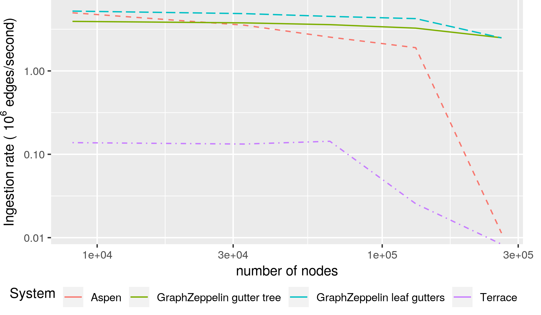
(b) Aspen and Terrace perform poorly on disk while GraphZeppelin’s stream ingestion rate remains high.

Dataset	Aspen	Terrace	Gutter Tree	Leaf-Only Gutters
kron13	$0.041$	$0.126$	$0.02$	$0.02$
kron15	$0.202$	$0.800$	$0.10$	$0.10$
kron16	$0.746$	$1.260$	$0.22$	$0.19$
kron17	$3.11$	N/A	$0.44$	$0.42$
kron18	N/A	N/A	$97.5$	$103$

(c) CC computation time after stream ingestion.

Figure 12. GraphZeppelin remains fast even when its data structures are stored on disk, unlike Aspen and Terrace.

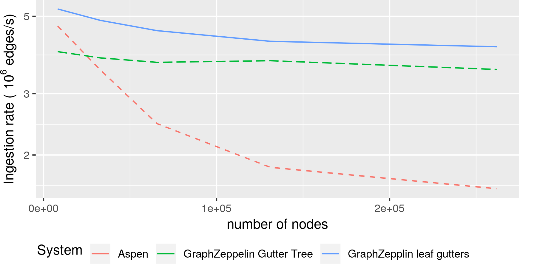
Figure 13. GraphZeppelin is faster than Aspen and Terrace even when all data structures fit in RAM.

In RAM, GraphZeppelin’s ingestion rate is higher than Aspen’s on all Kronecker streams. We summarize these results in Figure 13. Notably, on kron18 GraphZeppelin ingests 4.09 million updates per second, nearly three times faster than Aspen. GraphZeppelin ingests more than an order of magnitude faster than Terrace on these streams, so we omit it from the figure.

6.3. GraphZeppelin is Reliable

GraphZeppelin’s sketching algorithm is not deterministically correct: it has a nonzero failure probability, which is guaranteed to be at most $1/V^{c}$ for some constant $c$. To establish that failures do not occur in practice, we compared GraphZeppelin with an in-memory adjacency matrix stored as a bit vector. Specifically, we applied stream updates to GraphZeppelin and the adjacency matrix and periodically queried GraphZeppelin and compared its results with the output of running Kruskal’s algorithm on the adajacency matrix. We performed 1000 such correctness checks each on the kron17, p2p-gnutella, rec-amazon, google-plus, and web-uk streams. No failures were ever observed. While our algorithm’s performance is optimized for dense graphs, this experiment demonstrates that it succeeds with high probability for both dense and sparse graphs.

6.4. GraphZeppelin is Highly Parallel

Due to the atomized nature of sketch updates, we expect stream ingestion to scale well on multi-core systems. We experimentally demonstrate this claim by varying the number of threads used for processing updates and observe a significant speed-up.

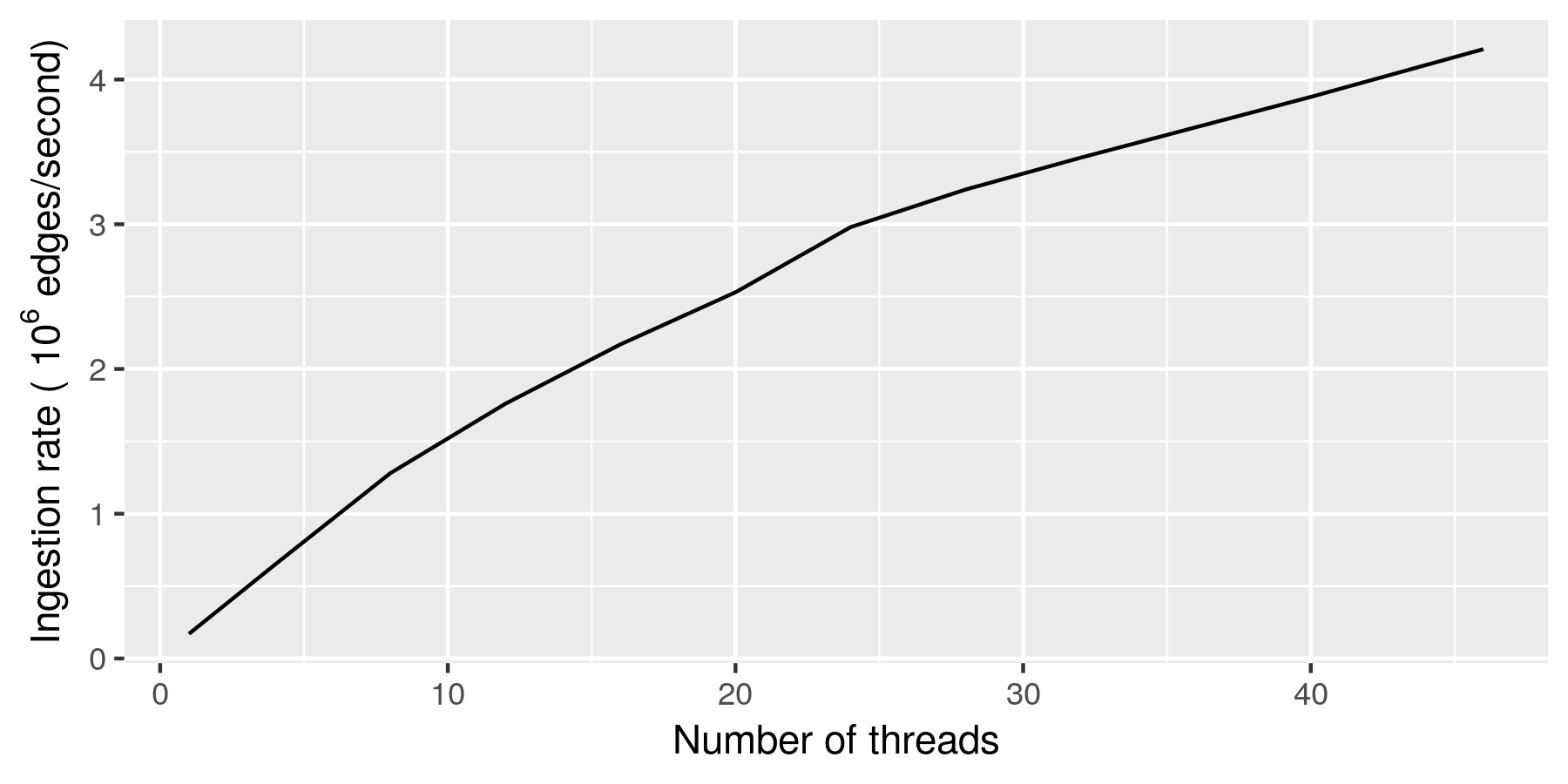
Figure 14. GraphZeppelin updates sketches in parallel, increasing ingestion rate by $26\times$ when using 46 threads.

Figure 14 shows the ingestion rate of GraphZeppelin as the number of threads processing the kron17 graph stream increases. The threads are given a pool of $64\textsc{GB}$ RAM so that the parallel performance can be measured without memory contention. To avoid external memory accesses, we use leaf-only gutters for buffering. The per-thread increase in ingestion rate is significant; the ingestion rate for 46 threads is approximately 26 times higher than that of a single thread. Additionally, at 46 threads the marginal ingestion rate is still positive, suggesting that adding more threads would further increase performance.

We also experimentally determined that a group size of one gives the best performance with our combination of machine and inputs.

6.5. GraphZeppelin Buffering Facilitates Parallelism and I/O Efficiency

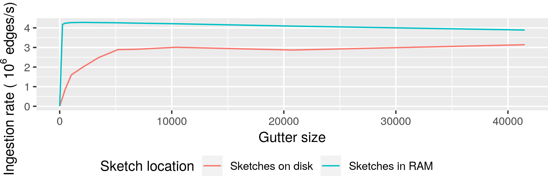
Figure 15. GraphZeppelin gutter size vs ingestion speed.

Applying sketch updates is highly scaleable, but only if updates are buffered and applied in batches. When sketches are stored on disk, processing each update individually requires $\Omega(1)$ IOs. Additionally, cache contention and thread synchronization bottleneck the ingestion rate even when sketches are in RAM. For these reasons we retain buffers of a constant factor $f$ of the node-sketch size.

Figure 15 summarizes the ingestion rate of GraphZeppelin on the kron17 stream for different values of $f$ when the sketches are stored in RAM and when they are stored on disk. GraphZeppelin is given 46 Graph Workers and a group size of 1. With buffers of size 1 (no buffering), GraphZeppelin ingests 130,000 updates per second in RAM, 33 times slower than when $f=.10$. On SSD, the ingestion rate is only 2000 insertions per second, 3 orders of magnitude slower than peak on-disk performance.

When the sketches fit in RAM, performance increases rapidly indicating that $f$ can be quite small while providing a high ingestion rate. However, once memory requirements exceed main memory, $f$ must be larger to offset disk IOs. To achieve an ingestion rate within 5% of peak performance on kron17, $f$ as small as $0.01$ is sufficient for entirely in RAM computation, while $f=.50$ is required when node sketches partially reside on disk.

6.6. Connectivity Queries are Fast

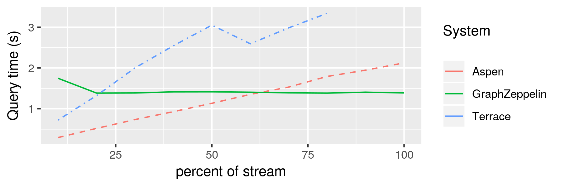
(a) In-memory query times.

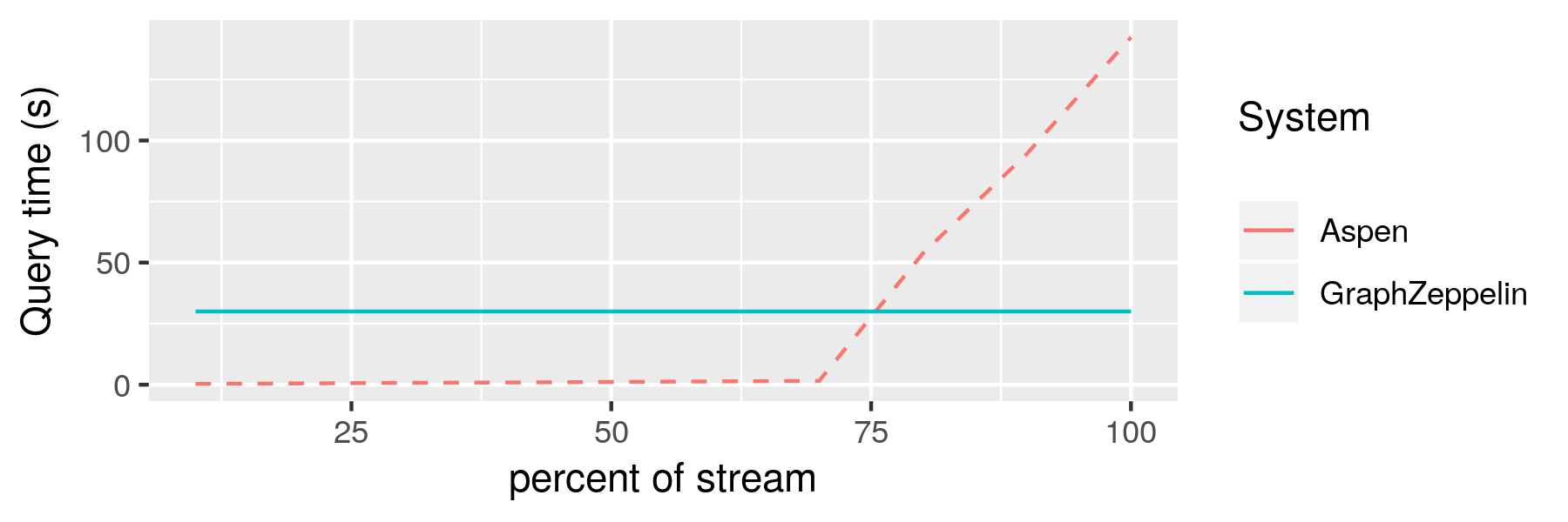
(b) On-disk query times.

Figure 16. GraphZeppelin query performance is comparable to or better than Aspen and Terrace for dense graphs.

We show experimentally that GraphZeppelin gives comparable query performance to Aspen and Terrace on dense graphs when all systems’ data structures fit in RAM. When their data structures reside on disk, GraphZeppelin answers queries more than five times faster than Aspen (and Terrace ingests too slowly to test).

GraphZeppelin’s buffering strategies create a tradeoff between stream-ingestion rate and query latency. When GraphZeppelin receives a connectivity query, it must process remaining stream updates in its buffering system before computing connectivity using Boruvka’s algorithm. Large buffers improve stream-ingestion rate (see Section 6.5), particularly when sketches are stored on disk, but this comes at the cost of increased query latency since these large buffers must be emptied. For the same reasons, small buffers improve query latency but may decrease ingestion rate.

Figure 16(a) compares the query latency of GraphZeppelin, Aspen, and Terrace on the kron17 stream where connectivity queries are issued every 10% of the way through the stream. In this experiment GraphZeppelin used small 400-byte leaf-only buffers, enough space for 100 stream updates. At the beginning of the stream, when the graph is sparser, both Aspen and Terrace answer queries more quickly than GraphZeppelin. As the stream progresses and the graph becomes denser, GraphZeppelin’s query time stays constant while Aspen’s and Terrace’s increase. By 70% of the way through the stream GraphZeppelin is fastest. Even with GraphZeppelin’s small buffer size its ingestion rate was 3.95 million per second, twice as fast as Aspen and almost 100 times faster than Terrace.

Figure 16(b) compares the query latency of GraphZeppelin and Aspen when RAM is limited to 12GiB, forcing both systems to store part of their data structures on disk. Terrace ingests too slowly given only 12GiB of RAM to be included in the experiment. In this experiment GraphZeppelin used 8.3 KB leaf-only buffers (one-tenth of sketch size). GraphZeppelin takes 24 seconds to perform queries regardless of graph density. Aspen’s queries are fast until the graph is too dense to fit in RAM; its last query takes 142 seconds, five times slower than GraphZeppelin. Notably, GraphZeppelin maintains an ingestion rate of 4.15 million updates per second, 46 times faster than Aspen. Both systems spend the majority of time on insertions, where GraphZeppelin’s advantages come through.

7. Related Work

Graph Streaming Systems.

Existing graph stream processing systems are designed primarily to handle updates in batches consisting entirely of insertions or entirely of deletions. Streaming systems that process updates in batches are generally divided into two categories. The first (which includes Terrace) consists of those systems which finish ingestion prior to beginning queries and finish queries prior to accepting any additional edges (terrace, ; ammar2018distributed, ; busato2018hornet, ; ediger2012stinger, ; murray2016incremental, ; sengupta2016graphin, ; sengupta2017evograph, ). The second (which includes Aspen) allows updates to be applied asynchronously by periodically taking “snapshots” of the graph during ingestion to be used in conducting queries (aspen, ; cheng2012kineograph, ; iyer2015celliq, ; iyer2016time, ; macko2015llama, ).

The batching employed in these systems amortizes the cost of applying updates, but also limits the granularity at which insertions and deletions may be interspersed during ingestion. In contrast, GraphZeppelin allows for insertions and deletions to be arbitrarily interspersed during ingestion without sacrificing query correctness.

External Memory Systems.

There is a rich literature of graph processing systems process static graphs in external memory. Some such systems store the entire graph out-of-core (KyrolaBlGu12, ; han2013turbograph, ; zhu2015gridgraph, ; maass2017mosaic, ; zhang2018wonderland, ), and others are semi-external memory systems that maintain only the vertex-set in RAM (roy2013x, ; zheng2015flashgraph, ; yuan2016pathgraph, ; liu2017graphene, ; ai2018clip, ). Some systems provide (at least theoretical) design extensions to handle queries on graphs with insert-only updates (KyrolaBlGu12, ; zhang2018wonderland, ; vora2016load, ; cheng2015venus, ; vora2019lumos, ), but to the best of our knowledge GraphZeppelin is the first to leverage external-memory effectively in the streaming model of insertions and deletions.

8. Conclusion

GraphZeppelin computes the connected components of graph streams using space asymptotically smaller than an explicit representation of the graph. It is based on CubeSketch, a new $\ell_{0}$-sketching data structure that outperforms the state of the art on graph-streaming workloads. This new sketching technique allows GraphZeppelin to process larger, denser graphs than existing graph-streaming systems given a fixed RAM budget and to ingest these graph streams more quickly. Even when GraphZeppelin’s sketch data structures are too large to fit in RAM, its work-buffering strategies allow it to process graph streams on SSD at the cost of a only small decrease in ingestion rate. Thus, GraphZeppelin is simultaneously a space-optimal graph semi-streaming algorithm and an I/O-efficient external-memory algorithm.

The small space complexity of GraphZeppelin’s linear sketch is optimized for large, dense graphs, unlike prior graph-processing systems, which often focus on sparse graphs. Thus, GraphZeppelin demonstrates that computational questions on graphs once thought intractably large and dense are now within reach.

Currently large, dense graphs are studied rarely and at great cost on large high-performance clusters (facebookdense, ). Since GraphZeppelin’s sketches can be updated independently (Section 5.1), we believe that they can be partitioned throughout a distributed cluster without sacrificing stream ingestion rate.

GraphZeppelin illustrates that additional algorithmic improvements help make graph semi-steaming algorithms into a powerful engineering tool by reducing the update-time complexity and allowing sketches to be stored efficiently on SSD. These techniques may generalize to other graph-analytics problems.

Acknowledgments

References

- [1] J. Abello, A. L. Buchsbaum, and J. R. Westbrook. A functional approach to external graph algorithms. Algorithmica, 32(3):437–458, 2002.
- [2] K. Ahn, S. Guha, and A. McGregor. Graph sketches: Sparsification, spanners, and subgraphs. Proceedings of the ACM SIGACT-SIGMOD-SIGART Symposium on Principles of Database Systems, 03 2012.
- [3] K. J. Ahn, S. Guha, and A. McGregor. Analyzing graph structure via linear measurements. In Proceedings of the twenty-third annual ACM-SIAM symposium on Discrete Algorithms, pages 459–467. SIAM, 2012.
- [4] Z. Ai, M. Zhang, Y. Wu, X. Qian, K. Chen, and W. Zheng. Clip: A disk i/o focused parallel out-of-core graph processing system. IEEE Transactions on Parallel and Distributed Systems, 30(1):45–62, 2018.
- [5] R. Albert. Scale-free networks in cell biology. Journal of cell science, 118(21):4947–4957, 2005.
- [6] S. Allegretti, F. Bolelli, M. Cancilla, and C. Grana. Optimizing gpu-based connected components labeling algorithms. In 2018 IEEE International Conference on Image Processing, Applications and Systems (IPAS), pages 175–180, 2018.
- [7] K. Ammar, F. McSherry, S. Salihoglu, and M. Joglekar. Distributed evaluation of subgraph queries using worstcase optimal lowmemory dataflows. arXiv preprint arXiv:1802.03760, 2018.
- [8] J. Ang, B. W. Barrett, K. B. Wheeler, and R. C. Murphy. Introducing the graph 500. 2010.
- [9] L. Arge. The buffer tree: A new technique for optimal i/o-algorithms (extended abstract). In University of Aarhus, pages 334–345. Springer-Verlag, 1995.
- [10] T. Y. Berger-Wolf and J. Saia. A framework for analysis of dynamic social networks. In Proceedings of the 12th ACM SIGKDD International Conference on Knowledge Discovery and Data Mining, KDD ’06, pages 523–528, New York, NY, USA, 2006. Association for Computing Machinery.
- [11] I. Bordino and D. Donato. Dynamic characterization of a large web graph.
- [12] G. S. Brodal, R. Fagerberg, D. Hammer, U. Meyer, M. Penschuck, and H. Tran. An experimental study of external memory algorithms for connected components. In 19th International Symposium on Experimental Algorithms (SEA 2021). Schloss Dagstuhl-Leibniz-Zentrum für Informatik, 2021.
- [13] L. Buš and P. Tvrdik. A parallel algorithm for connected components on distributed memory machines. In European Parallel Virtual Machine/Message Passing Interface Users’ Group Meeting, pages 280–287. Springer, 2001.
- [14] F. Busato, O. Green, N. Bombieri, and D. A. Bader. Hornet: An efficient data structure for dynamic sparse graphs and matrices on gpus. In 2018 IEEE High Performance extreme Computing Conference (HPEC), pages 1–7. IEEE, 2018.
- [15] J. Cheng, Q. Liu, Z. Li, W. Fan, J. C. Lui, and C. He. Venus: Vertex-centric streamlined graph computation on a single pc. In 2015 IEEE 31st International Conference on Data Engineering, pages 1131–1142. IEEE, 2015.
- [16] R. Cheng, J. Hong, A. Kyrola, Y. Miao, X. Weng, M. Wu, F. Yang, L. Zhou, F. Zhao, and E. Chen. Kineograph: taking the pulse of a fast-changing and connected world. In Proceedings of the 7th ACM european conference on Computer Systems, pages 85–98, 2012.
- [17] Y.-J. Chiang, M. T. Goodrich, E. F. Grove, R. Tamassia, D. E. Vengroff, and J. S. Vitter. External-memory graph algorithms. In Proc. 6th annual ACM-SIAM Symposium on Discrete Algorithms (SODA), pages 139–149. Society for Industrial and Applied Mathematics, 1995.
- [18] A. Ching, S. Edunov, M. Kabiljo, D. Logothetis, and S. Muthukrishnan. One trillion edges: Graph processing at facebook-scale. Proc. VLDB Endow., 8(12):1804–1815, aug 2015.
- [19] Y. Collet. xxhash-extremely fast non-cryptographic hash algorithm. URL https://github. com/Cyan4973/xxHash, 2016.
- [20] G. Cormode and D. Firmani. A unifying framework for -sampling algorithms. Distributed and Parallel Databases, 32, 09 2014.
- [21] L. Dhulipala, G. Blelloch, and J. Shun. Low-latency graph streaming using compressed purely-functional trees. Proceedings of the ACM SIGPLAN Conference on Programming Language Design and Implementation (PLDI).
- [22] D. Ediger, R. McColl, J. Riedy, and D. A. Bader. Stinger: High performance data structure for streaming graphs. In 2012 IEEE Conference on High Performance Extreme Computing, pages 1–5. IEEE, 2012.
- [23] M. Ester, H.-P. Kriegel, J. Sander, and X. Xu. A density-based algorithm for discovering clusters in large spatial databases with noise. pages 226–231. AAAI Press, 1996.
- [24] Y. Fang, R. Cheng, S. Luo, and J. Hu. Effective community search for large attributed graphs. Proc. VLDB Endow., 9(12):1233–1244, Aug. 2016.
- [25] Y. Fang, R. Cheng, S. Luo, and J. Hu. Effective community search for large attributed graphs. Proc. VLDB Endow., 9(12):1233–1244, Aug. 2016.
- [26] J. Feigenbaum, S. Kannan, A. McGregor, S. Suri, and J. Zhang. On graph problems in a semi-streaming model. Theor. Comput. Sci., 348(2):207–216, Dec. 2005.
- [27] E. Georganas, R. Egan, S. Hofmeyr, E. Goltsman, B. Arndt, A. Tritt, A. Buluç, L. Oliker, and K. Yelick. Extreme scale de novo metagenome assembly. SC ’18. IEEE Press, 2018.
- [28] J. Greiner. A comparison of parallel algorithms for connected components. In Proceedings of the sixth annual ACM symposium on Parallel algorithms and architectures, pages 16–25, 1994.
- [29] S. Guha, A. McGregor, and D. Tench. Vertex and hyperedge connectivity in dynamic graph streams. In PODS, pages 241–247. ACM, 2015.
- [30] W.-S. Han, S. Lee, K. Park, J.-H. Lee, M.-S. Kim, J. Kim, and H. Yu. Turbograph: a fast parallel graph engine handling billion-scale graphs in a single pc. In Proceedings of the 19th ACM SIGKDD international conference on Knowledge discovery and data mining, pages 77–85, 2013.
- [31] L. He, Y. Chao, K. Suzuki, and K. Wu. Fast connected-component labeling. Pattern recognition, 42(9):1977–1987, 2009.
- [32] L. He, X. Ren, Q. Gao, X. Zhao, B. Yao, and Y. Chao. The connected-component labeling problem: A review of state-of-the-art algorithms. Pattern Recognition, 70:25–43, 2017.
- [33] M. M. Hossam, A. E. Hassanien, and M. Shoman. 3d brain tumor segmentation scheme using k-mean clustering and connected component labeling algorithms. In 2010 10th International Conference on Intelligent Systems Design and Applications, pages 320–324, 2010.
- [34] A. Iyer, L. E. Li, and I. Stoica. Celliq: Real-time cellular network analytics at scale. In 12th USENIX Symposium on Networked Systems Design and Implementation (NSDI 15), pages 309–322, 2015.
- [35] A. P. Iyer, L. E. Li, T. Das, and I. Stoica. Time-evolving graph processing at scale. In Proceedings of the fourth international workshop on graph data management experiences and systems, pages 1–6, 2016.
- [36] J. Jung, K. Shin, L. Sael, and U. Kang. Random walk with restart on large graphs using block elimination. ACM Transactions on Database Systems (TODS), 41(2):1–43, 2016.
- [37] U. Kang and C. Faloutsos. Beyond ’caveman communities’: Hubs and spokes for graph compression and mining. pages 300–309, 12 2011.
- [38] U. Kang, M. McGlohon, L. Akoglu, and C. Faloutsos. Patterns on the connected components of terabyte-scale graphs. pages 875–880, 12 2010.
- [39] M. Korn, D. Sanders, and J. Pauli. Moving object detection by connected component labeling of point cloud registration outliers on the gpu. In VISIGRAPP (6: VISAPP), pages 499–508, 2017.
- [40] A. Krishnamurthy, S. Lumetta, D. E. Culler, and K. Yelick. Connected components on distributed memory machines. Third DIMACS Implementation Challenge, 30:1–21, 1997.
- [41] A. Kyrola, G. Blelloch, and C. Guestrin. Grapchi: Large-scale graph computation on just a pc. In 10th USENIX Symposium on Operating Systems Design and Implementation, pages 31–46. USENIX, 2012.
- [42] W. Lee, J. J. Lee, and J. Kim. Social network community detection using strongly connected components. In Pacific-Asia Conference on Knowledge Discovery and Data Mining, pages 596–604. Springer, 2014.
- [43] J. Leskovec, L. A. Adamic, and B. A. Huberman. The dynamics of viral marketing. ACM Transactions on the Web (TWEB), 1(1):5–es, 2007.
- [44] J. Leskovec and A. Krevl. SNAP Datasets: Stanford large network dataset collection. http://snap.stanford.edu/data, June 2014.
- [45] Y. Lim, U. Kang, and C. Faloutsos. Slashburn: Graph compression and mining beyond caveman communities. IEEE Transactions on Knowledge and Data Engineering, 26(12):3077–3089, 2014.
- [46] Y. Lim, W.-J. Lee, H.-J. Choi, and U. Kang. Discovering large subsets with high quality partitions in real world graphs. In 2015 International Conference on Big Data and Smart Computing (BIGCOMP), pages 186–193. IEEE, 2015.
- [47] Y. Lim, W.-J. Lee, H.-J. Choi, and U. Kang. Mtp: discovering high quality partitions in real world graphs. World Wide Web, 20(3):491–514, 2017.
- [48] H. Liu and H. H. Huang. Graphene: Fine-grained IO management for graph computing. In 15th USENIX Conference on File and Storage Technologies (FAST 17), pages 285–300, 2017.
- [49] S. Maass, C. Min, S. Kashyap, W. Kang, M. Kumar, and T. Kim. Mosaic: Processing a trillion-edge graph on a single machine. In Proceedings of the Twelfth European Conference on Computer Systems, pages 527–543, 2017.
- [50] P. Macko, V. J. Marathe, D. W. Margo, and M. I. Seltzer. Llama: Efficient graph analytics using large multiversioned arrays. In 2015 IEEE 31st International Conference on Data Engineering, pages 363–374. IEEE, 2015.
- [51] J. J. McAuley and J. Leskovec. Learning to discover social circles in ego networks. In NIPS, volume 2012, pages 548–56. Citeseer, 2012.
- [52] A. McGregor, D. Tench, S. Vorotnikova, and H. T. Vu. Densest subgraph in dynamic graph streams. In G. F. Italiano, G. Pighizzini, and D. T. Sannella, editors, Mathematical Foundations of Computer Science 2015, pages 472–482, Berlin, Heidelberg, 2015. Springer Berlin Heidelberg.
- [53] D. Medini, A. Covacci, and C. Donati. Protein homology network families reveal step-wise diversification of type iii and type iv secretion systems. PLoS computational biology, 2(12):e173, 2006.
- [54] D. G. Murray, F. McSherry, M. Isard, R. Isaacs, P. Barham, and M. Abadi. Incremental, iterative data processing with timely dataflow. Communications of the ACM, 59(10):75–83, 2016.
- [55] S. Muthukrishnan. Data streams: Algorithms and applications. Foundations and Trends® in Theoretical Computer Science, 1(2):117–236, 2005.
- [56] J. Nelson and H. Yu. Optimal lower bounds for distributed and streaming spanning forest computation. In Proceedings of the Thirtieth Annual ACM-SIAM Symposium on Discrete Algorithms, pages 1844–1860. SIAM, 2019.
- [57] J. Nešetřil, E. Milková, and H. Nešetřilová. Otakar borůvka on minimum spanning tree problem translation of both the 1926 papers, comments, history. Discrete Math., 233(1–3):3–36, Apr. 2001.
- [58] S. Nurk, D. Meleshko, A. Korobeynikov, and P. Pevzner. Metaspades: A new versatile metagenomic assembler. Genome Research, 27:gr.213959.116, 03 2017.
- [59] OpenMP Architecture Review Board. OpenMP Application Programming Interface, 5th edition, Nov. 2018.
- [60] P. Pandey, B. Wheatman, H. Xu, and A. Buluc. Terrace: A hierarchical graph container for skewed dynamic graphs. In Proceedings of the 2021 International Conference on Management of Data, pages 1372–1385, 2021.
- [61] M. M. A. Patwary, D. Palsetia, A. Agrawal, W.-k. Liao, F. Manne, and A. Choudhary. A new scalable parallel dbscan algorithm using the disjoint-set data structure. In SC ’12: Proceedings of the International Conference on High Performance Computing, Networking, Storage and Analysis, pages 1–11, 2012.
- [62] A. Pothen and C.-J. Fan. Computing the block triangular form of a sparse matrix. 16(4):303–324, Dec. 1990.
- [63] M. Ripeanu, I. Foster, and A. Iamnitchi. Mapping the gnutella network: Properties of large-scale peer-to-peer systems and implications for system design. arXiv preprint cs/0209028, 2002.
- [64] R. A. Rossi and N. K. Ahmed. The network data repository with interactive graph analytics and visualization. In AAAI, 2015.
- [65] A. Roy, I. Mihailovic, and W. Zwaenepoel. X-stream: Edge-centric graph processing using streaming partitions. In Proceedings of the Twenty-Fourth ACM Symposium on Operating Systems Principles, pages 472–488, 2013.
- [66] S. Sahu, A. Mhedhbi, S. Salihoglu, J. Lin, and M. T. Özsu. The ubiquity of large graphs and surprising challenges of graph processing. Proc. VLDB Endow., 11(4):420–431, Dec. 2017.
- [67] D. Sengupta and S. L. Song. Evograph: On-the-fly efficient mining of evolving graphs on gpu. In International Supercomputing Conference, pages 97–119. Springer, 2017.
- [68] D. Sengupta, N. Sundaram, X. Zhu, T. L. Willke, J. Young, M. Wolf, and K. Schwan. Graphin: An online high performance incremental graph processing framework. In European Conference on Parallel Processing, pages 319–333. Springer, 2016.
- [69] H. Thornquist, E. Keiter, R. Hoekstra, D. Day, and E. Boman. A parallel preconditioning strategy for efficient transistor-level circuit simulation. pages 410–417, 01 2009.
- [70] S. van Dongen. Graph clustering by flow simulation. Technical report, 2000.
- [71] J. S. Vitter. External memory algorithms and data structures: Dealing with massive data. ACM Computing Surveys, 33:2001, 2001.
- [72] K. Vora. LUMOS: Dependency-driven disk-based graph processing. In 2019 USENIX Annual Technical Conference, pages 429–442, 2019.
- [73] K. Vora, G. Xu, and R. Gupta. Load the edges you need: A generic i/o optimization for disk-based graph processing. In 2016 USENIX Annual Technical Conference, pages 507–522, 2016.
- [74] D. Wen, L. Qin, Y. Zhang, L. Chang, and X. Lin. Efficient structural graph clustering: An index-based approach. The VLDB Journal, 28(3):377–399, June 2019.
- [75] D. Wen, L. Qin, Y. Zhang, L. Chang, and X. Lin. Efficient structural graph clustering: An index-based approach. The VLDB Journal, 28(3):377–399, June 2019.
- [76] M. Wu, X. li, C.-K. Kwoh, and S.-K. Ng. A core-attachment based method to detect protein complexes in ppi networks. BMC bioinformatics, 10:169, 02 2009.
- [77] P. Yuan, C. Xie, L. Liu, and H. Jin. Pathgraph: A path centric graph processing system. IEEE Transactions on Parallel and Distributed Systems, 27(10):2998–3012, 2016.
- [78] M. Zhang, Y. Wu, Y. Zhuo, X. Qian, C. Huan, and K. Chen. Wonderland: A novel abstraction-based out-of-core graph processing system. ACM SIGPLAN Notices, 53(2):608–621, 2018.
- [79] D. Zheng, D. Mhembere, R. Burns, J. Vogelstein, C. E. Priebe, and A. S. Szalay. Flashgraph: Processing billion-node graphs on an array of commodity ssds. In 13th USENIX conference on file and storage technologies (FAST 15), pages 45–58, 2015.
- [80] X. Zhu, W. Han, and W. Chen. Gridgraph: Large-scale graph processing on a single machine using 2-level hierarchical partitioning. In 2015 USENIX Annual Technical Conference.