Non-Parametric Stochastic Policy Gradient with Strategic Retreat for Non-Stationary Environment

Abstract

In modern robotics, effectively computing optimal control policies under dynamically varying environments poses substantial challenges to the off-the-shelf parametric policy gradient methods, such as the Deep Deterministic Policy Gradient (DDPG) and Twin Delayed Deep Deterministic policy gradient (TD3). In this paper, we propose a systematic methodology to dynamically learn a sequence of optimal control policies non-parametrically, while autonomously adapting with the constantly changing environment dynamics. Specifically, our non-parametric kernel-based methodology embeds a policy distribution as the features in a non-decreasing Euclidean space, therefore allowing its search space to be defined as a very high (possible infinite) dimensional RKHS (Reproducing Kernel Hilbert Space). Moreover, by leveraging the similarity metric computed in RKHS, we augmented our non-parametric learning with the technique of AdaptiveH— adaptively selecting a time-frame window of finishing the optimal part of whole action-sequence sampled on some preceding observed state. To validate our proposed approach, we conducted extensive experiments with multiple classic benchmarks and one simulated robotics benchmark equipped with dynamically changing environments. Overall, our methodology has outperformed the well-established DDPG and TD3 methodology by a sizeable margin in terms of learning performance.

I INTRODUCTION

Reinforcement Learning (RL) has revolutionized the process of learning optimal action mapping policies in diverse problem domains ranging from video games[1] to robotic navigation[2]. Among many Deep Reinforcement Learning (DRL) algorithms, DDPG (Deep Deterministic Policy Gradient) [3] and its upgraded variant TD3 (Twin Delayed Deep Deterministic Policy Gradient) [4], have attained immense successes in robotics through strategically combining optimal deterministic policy search algorithms and value-function learning. Despite many successes of DRL in robotic learning, the vast majority of these studies, however, restrictively assume the model of their operating environments to be static. In fact, while extensive research has been conducted on policy gradient methods in order to handle real-world high dimensional continuous space environments, much less attention has been dedicated to formulate algorithms to handle non-stationary systems.

Unfortunately, real-world environments in robotics are typically nonstationary and evolving, therefore governed by dynamically changing transition dynamics due to some totally imperceptible causes. As such, learning optimal control policy under dynamically varying environments with conventional methodologies, such as DDPG or TD3, becomes both computationally intensive and quite time-consuming. Specifically, while interplaying with a dynamically self-altering environment, actions suggested by a deterministic policy based on the preceding state observation become outdated as the state-space is continuously evolving. On the contrary, by learning a stochastic policy in a continuously evolving environment, more probable actions can be sampled from the policy. Moreover, in case of deterministic way of learning, it is assumed that a stationary transition dynamics and reward distribution exist in the environment [3, 5]. As a result, deterministic policy gradient method performs suboptimally, when the learning algorithm is exposed to problems where transition functions and reward distributions are changing in a non-deterministic fashion. Comparatively, a probabilistic approach for action sampling from a policy distribution can suggest actions compatible to handle the stochasticity of the dynamic environment. In particular, probabilistic algorithms for handling optimization problems or perception learning often exhibit robustness to sensory irregularities, random perturbations and stochastic nature of environments and scale much better to the complex environments, where the agent need to handle unknown uncertainty in much robust and adaptive way [6].

To overcome all these thorny challenges fundamentally caused by the non-stationarity of underlying environment, we formulate the scheme of adaptively learning sequence of action-mapping functionals by embedding the functionals into a vector-valued kernel space instead of a fixed parametric space and representing policy distributions defined over a high (possible infinite) dimensional RKHS [7]. In this paper, we develop a new class of non-parametric policy gradient methods [8] which optimally ensures a gradient ascending direction while optimizing and adaptively executing such actions compatible with the concurrent dynamics of the environment. We validate both theoretically and experimentally that our proposed approach can handle non-stationary environments with hidden, but bounded, degree of dynamic evolution. In most cases, such an upper-bound on the non-stationary transition dynamics is reasonably ensured by considering that the evolution rate of the non-stationary MDPs are bounded by Lipschitz Continuity assumption[8],[9].

Why Non-Parametric Reinforcement Learning? — In a real-world robotic setting, policy computation and policy inference possess certain latency and it is impossible to pause the environment in the continuous stream of operating phase. So, an adaptive learning framework is highly required to handle dynamically varying transition distribution and reward function through updating policy distribution in a more frequent policy update fashion. But unfortunately, in parametric setting like DDPG, finding a gradient similarity metric to find an adaptive termination point for frequent policy updates is mathematically very difficult and often gradients can not be easily estimated, which can be easily done in an RKHS based non-parametric learning framework[7], [8]. Parametric methods also impose two major disadvantages. Firstly, for a parametric model like DDPG, it is very difficult to initialize a suitable prior parameter matrix as picking too large matrix can be computationally expensive or picking too small will be unable to fit the complex policies need to learn for action mapping [7]. Secondly, when the dimension of problem goes higher, the policy update in algorithm like DDPG grows exponentially. Such update can cause exploding gradients while dealing with unbounded system variances. To address theses issues, non-parametric policy learning leverages transition distributions as kernel embeddings in an RKHS whose complexity remains linear with dimensionality of problem space. Non-parametric representation of control policies can be adaptive as RKHS based kernel trick enables the agent to learn complex, but sufficient, representation of stochastic control policies when required.

Why Strategic Retreats or Adaptive-H? — Unfortunately, kernel based non-parametric learning possesses one major disadvantage. Non-parametric method requires a lot of training data to accurately model the action-mapping functions. RL itself is a data-hungry method. As a result, the kernel matrix, often stated as Gram Matrix[10] becomes huge in dimension and, in turn, brings the problem of memory-explosion. Thus, the learning rate for optimization becomes very slow and kernel centers in the kernel dictionary increase exponentially with more experiences from the environment. Since, a part of sampled action-trajectory becomes obsolete as the state-space evolves, the problem of memory-explosion can be prevented by adaptively presetting a termination trigger to stop non-optimal action execution in an episodic trajectory and perform policy update. Thus, the algorithm can be made truly scalable for very large dimensional problems and can be sample-efficient by truncating the full trajectories at optimal timing. We term this new formulation in accordance with a non-parametric policy gradient as AdaptiveH

Why Combining RKHS Method and Strategic Retreats? — The policy gradients with respect to action-mapping mean functional can be easily and efficiently estimated in an RKHS following Fréchet Derivative[7]. Such gradient estimation is not mathematically sound in parametric TD3 and DDPG method. Respectively, since policy distributions are considered as elements of an RKHS and RKHS itself inherits all properties of a vector space, a dot product based similarity metric [8] can be efficiently utilized to guide the policy search method. By adopting this similarity metric between consecutive gradient updates, our agent adaptively develop sequence of control polices in a completely non-stationary setting with potentially bounded variance in system dynamics. Moreover, we mention the theoretical convergence guarantee to the fixed point solution by proving that dynamic regret term becomes a sub-martingale through continual policy learning. For reward maximization, policy gradients should move into an ascent direction during the optimization process to reach global maxima point. Formulated on this concept, we consecutively measure the dot product between two gradient updates. If the result of the dot product diverges from being a positive number, the following gradients are deviating from an ascent direction. At that instance, our agent pre-maturely aborts action-execution and upgrades itself to a new policy. Thus, we adaptively tune a action-execution window $H$ after which less important actions are not fully finished. Such adjustable and frequent policy update brings about sequence of optimal control policies and this scheme can not be done easily in deterministic policy search method.

Contributions :

• We proposed a non-parametric policy gradient framework which can adaptively generate sequence of control policies to handle dynamically varying real-world scenarios.

• We introduced both theoretical guarantees and experimental proofs that by premature action stopping and frequent policy update through a dot-product based similarity metric in RKHS, our proposed approach can speed up the learning process and enhance sample-efficiency.

• We also validate that our proposed approach can exhibit better performance than state-of-the-art parametric DRL algorithms like TD3 and DDPG in non-stationary environments.

Figure 1: (a) Sketch of optimal Action Selection by estimating Adaptive-H period window and sequence of policy updates. (b) Overview of Algorithmic steps for inner-product based gradient ascent direction assurance for maximizing expected rewards.

II RELATED WORKS

Non-Stationary Reinforcement Learning— Very recently, a lot of attention have been drawn to address non-stationary environments through DRL. For instance, [11] proposed online Context-Q learning, based on change point detection method[12], that stores various policy distributions from varying contexts occured in known model-change patterns. Another work [9] investigated Non-Stationary MDPs (NS-MDP) by considering the non-stationary environment as an adversary to the learning agent and constructed a model based tree search algorithm close to traditional minimax search algorithm. In [13], authors built probabilistic hierarchical model to present non-stationary Markov chain with sequence of latent variables and used variational inference to set a lower bound for log probability of evidences observed.

Non-parametric Reinforcement Learning— RKHS based non-parametric reinforcement learning and associated rich function class has been used previously to generate stochastic policies. For instance, [7] proposed compact representation of policy within an RKHS with no need of remetrization of abstract feature space and showed a non-parametric actor-critic framework through efficient sparsification method in RKHS. The authors in [14] and [8] showed more attention to device a stochastic policy gradient method by plugging unbiased stochastic policy gradient computed in an RKHS and build a theoretical framework of convergence to a neighborhood of critical points.

In general, recent methods focused to accurately outline control policies in a fixed parameter space while non-parametric methods tried to build a framework for policy representation in an RKHS to exploit its rich function space. In our work, we employed inner-product property of RKHS to build up an adaptive checkpoint detection method for learning optimal control policies in a dynamically changing environment.

III PRELIMINARIES

We design the problem formulation in the context of non-stationary RL where an agent operates in an environment with unknown non-stationarity, with a motive to learn optimal control policies to maximize the agent’s long-term utility. This interaction with non-stationary environment is lately modelled as Non-Stationary Markov Decision Process (NS-MDP) [9], [15], [16], [11]. Many real-world non-stationary environments have a tractable state-space but it is practically impossible to draw an assumption on how its future evolution will look like [17],[9]. Based on this hypothesis, the agent accumulate snapshots of current model after each action is executed, but it can not easily track the dynamic variance in state distribution. We target to build an adaptive learning framework for handling such dynamic variance. In section III-A, we formulate the layout of NS-MDP framework and in section III-B we explicitly mention the bottlenecks of parametric approach for computing policy integrals with deterministic gradients. In section III-C, we mention non-parametric policy gradient methods formulated over RKHS.

III-A NS-MDP Composition

Let $\mathcal{P}(\mathcal{S})$ be a set of probability distribution for each state $s\in\mathcal{S}$, and the NS-MDP instance be a tuple $(\mathcal{S,A,T},\{r_{t}\}_{t\in\mathcal{T}},\{P_{t}\}_{t\in\mathcal{T}},P_{0})$ [9], where $\mathcal{S}$ and $\mathcal{A}$ represent the state and action spaces, $\mathcal{T}:\{1,2....,N\}$ represents each decision epoch when agent is interacting with the environment, $r_{t}(\cdot\mid a,s)\in\mathcal{P}(\mathcal{R})$ represents state-reward distribution over actions at decision epoch $t$; $P_{t}(\cdot\mid a,s)\in\mathcal{P}(\mathcal{S})$ is the state transition probability distribution at decision epoch $t$, which is non-stationary; and $P_{0}(\cdot)\in\mathcal{P}(\mathcal{S})$ is the probability distribution over initial state $s_{0}$. The agent selects actions using policy $\pi(\cdot\mid s)\in\mathcal{P}(\mathcal{A})$, which is a probability distribution over actions, conditioned over state $s$. The sequence of action selection given a state forms a Markov chain $\xi=(s_{0},a_{0},s_{1},a_{1},\dots,s_{T-1},a_{T-1},s_{T})$. The probability density function for $\xi$ is represented as $\operatorname{Pr}(\xi\mid\pi)=P_{0}(s_{0})\prod_{i=0}^{T-1}\pi(a_{i}\mid s_{i})P_{t}(s_{i+1}\mid s_{i},a_{i})$ and the discounted reward is defined by $R(\xi)=\sum_{i=0}^{T}\gamma^{t}r_{t}(s_{i},a_{i})$ where $\gamma$ is the discount factor.

III-B Bottlenecks in parametric deterministic policy learning

In the case of conventional stationary MDP setting with discounted reward function, there always exists a Markovian Deterministic stationary action-mapping policy[18]. In case of deterministic policy search algorithm like DDPG, the policy search is done by estimating the gradients over expected return, in form of Q-value function $Q^{\mu}(s,a)$, from of class of parameterized deterministic policies $\mu(\cdot|s,\theta),s\in\mathcal{S},\theta\in\Theta$ w.r.t parameter matrix $\theta$. The parameter matrix is adjusted by following the guidance provided by policy gradients computed as $\nabla_{\theta}J(\mu_{\theta})=\int_{\mathcal{S}}Pr(\xi|\mu_{\theta})\nabla_{\theta}\mu_{\theta}(s)\nabla_{a}Q^{\mu_{\theta}}(s,a)|_{a=\mu_{\theta}(s),s\sim\xi}ds$ [5]. Firstly, this integration only spans over visited state-space. As a result, a deterministic policy can not model the varying dynamics of a non-stationary environment. Secondly, deterministic estimation of policy gradients are unsound since it assumes that a stationary state distribution and reward function always exist in the MDP setting. This assumption makes the estimated gradients irrelevant if the reward distribution is likely evolving as time passes [19]. In such cases, a probabilistic approach such as stochastic policy calculation is more rigid to handle non-stationary transition dynamics.

In parametric cases, policies are given as linear functions over feature space $\phi(\cdot)$ as $\mu_{\theta}(\cdot)=\theta^{T}\phi(\cdot)$ or by non-linear approximators as $\mu_{\theta}(\cdot)=g(\theta^{T}\phi(\cdot))$. With a Euclidean Norm, it is very straightforward to compute policy gradients with respect to parameters $\theta$. But, there exists no apparent way to choose a scaling of these parameters. Besides, deficient parameter initialization slows down the learning rate and pre-conditioning of the priori becomes computationally expensive (detailed discussion in [7]).

III-C Non-Parametric Space for Gradient Estimation

To address the above issues with parametric approaches, we opt to design non-parametric stochastic policy learning framework with a non-decreasing vector-valued RKHS in this paper. First of all, now policy gradient is an entire function in RKHS, not limited by a fixed priori parameterization of the class. Thus, we can exploit a rich function class for adaptively learning a complex, but sufficient, representation for stochastic policies.

Here, we opt to represent policies as multivariate Gaussian models defined as a mapping function $h:\mathcal{S}\rightarrow\mathcal{A}$, where $h(s)$ belongs to a vector-valued RKHS $\mathcal{H}$ in which, $\forall h\in\mathcal{H},\ s\in\mathcal{S}\ \text{and}\ \mathbf{a}\in\mathbb{R}^{d}$, the reproducing property $\langle h(\cdot),\mathcal{K}(s,\cdot)\mathbf{a}\rangle_{\mathcal{H}}=h(s)^{T}\mathbf{a}$, holds true. Here, $\mathcal{K}(s,s^{\prime})$ is a matrix valued Gaussian kernel. Gaussian control policies can be expressed as

$$\pi_{h,\Sigma}(a|s)=\frac{1}{\sqrt{2\pi|\Sigma|}}e^{-\frac{(a-h(s))^{T}\Sigma^{-1}(a-h(s))}{2}}.$$ (1)

In this non-parametric learning paradigm, the learning objective will be finding the optimal mapping $h^{*}$ such that

$$\scriptsize h^{*}:=\operatorname*{argmax}_{h\in\mathcal{H}}J_{s_{0}}(h)=\operatorname*{argmax}_{h\in\mathcal{H}}\mathbf{E}\Big{[}\sum_{t=0}^{\infty}\gamma^{t}r(s_{t},a_{t})|h,s_{0}\Big{]}.$$ (2)

Similarly, the action-value function $Q(s,a;h)$ can be defined as $Q(s,a;h)=\mathbf{E}[\sum_{t=0}^{\infty}\gamma^{t}r(s_{t},a_{t})|h,s_{0},a_{0}]$. Furthermore, by utilizing the formulation of Fréchet Derivative as in [7], the gradient of $J_{s_{0}}(h,\cdot)$ with respect to functional $h$ yields

$$\scriptsize\nabla_{h}J_{s_{0}}(h,\cdot)=\frac{1}{1-\gamma}\mathbf{E}_{(s,a)\sim\rho_{s_{0}}(s,a)}\big{[}Q(s,a;h)\kappa(s,\cdot)\Sigma^{-1}(a-h(s))|h\big{]},$$ (3)

a function in $\mathcal{H}$, where $\rho_{s_{0}}(s,a):=\pi_{h}(a|s)(1-\gamma)\Sigma_{t=0}^{\infty}\gamma^{t}p(s_{t}|s_{0})=\pi_{h}(a|s)\rho_{s_{0}}(s)$. Finally, as the gradient ascent upgrades the mean functional as $h_{k+1}=h_{k}+\alpha_{t}\nabla_{h_{k}}J_{s_{0}}(h_{k},\cdot)$, Eq. (3) can be expressed as,

$$\nabla_{h}J_{s_{0}}(h,\cdot)={} \frac{1}{1-\gamma}\int\int Q(s,a;h)\kappa(s,\cdot)\Sigma^{-1}(a-h(s))\rho_{s_{0}}(s,a)dsda$$ (4)

$$={} \frac{1}{1-\gamma}\int D(s)\kappa(s,\cdot)\rho_{s_{0}}(s)ds,$$

where $D(s)=\int Q(s,a;h)\Sigma^{-1}(a-h(s))\pi_{h}(a|s)da$ following [8]. Moreover, modeling probability distributions in an RKHS (Eq. (4)) can be principally scaled by RKHS norm, which does not require to retain a parameter vector. We only rely on repositioning (vector-valued version of) kernels on the support of current snapshots of state-space to predict transition dynamics in evolutionary NS-MDP settings.

IV PROPOSED METHODOLOGY

At high level, our proposed AdaptiveH framework is based on Kernel based Value Approximation and non-parametric policy learning equipped with advantages from kernel based feature mapping within a defined RKHS which adaptively facilitates frequent policy updates when required in a dynamically challenging environment. We extend the theoretical basis described in subsection III-C by doing gradient estimation through kernel based high (possible infinite)-dimensional feature mapping and an inner-product based gradient direction checking for maximizing utility in a highly non-stationary environment. As shown in Fig.1, by only executing the optimal part of the whole trajectory and frequent policy update when required, we promise a sample-efficient learning in RKHS and faster to converge algorithm to handle dynamic variance in the system.

Considering the simulated agents working in dynamic environments modelled as NS-MDP setting, current policy $\pi_{h_{k}}(\cdot|s_{0})$ suggests an initial action sequence $\mathcal{A}=\{a_{0},a_{1},...,a_{n}\}$ based on current snapshot of MDP $\mathcal{M}_{0}$. But, since the transition dynamics of the NS-MDP setting and reward function is continually evolving through time, the agent sporadically experiences an urge to upgrade it previous policy $\pi_{h_{0}}(\cdot|s_{0})$ before even fully executing the already in-queue actions from previous policy. Our principal investigation is centered on this question on how to estimate the exact adaptive time-period window H at which the agent will pre-maturely retreat and upgrade to a new policy to handle hidden non-stationarity of the environment. In [20], this time-period H was kept as a fixed value while concurrently execution previous actions and learning new policies.

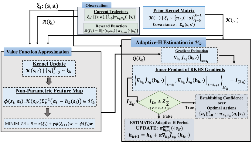
Figure 2: Detailed Algorithmic Approach for Adaptive-H estimation

Specifically, our approach (in Fig. 2) proposes a resolution to challenges of adaptively bisecting the whole sampled $\mathcal{A}$ into optimal $\mathcal{A}_{opt}$ and obsolete $\mathcal{A}_{left}$ parts by using similarity metric in RKHS. Thus, our agent frequently revisit the policy update after only executing those optimal actions compatible to the dynamic changes happened in the environment and our algorithm exhibits sample-efficiency and faster convergence in a NS-MDP setting. In particular to map our state-space into a high (possibly infinite)-dimensional RKHS, we construct diagonal matrix-valued Gaussian kernel, $\kappa_{\Sigma_{H}}(s,\cdot)$ with covariance matrix $\Sigma_{H}$ as

$$\scriptsize\kappa_{\Sigma_{H}}(s,s^{\prime})_{ii}=e^{\frac{{-(s-s^{\prime})^{T}\Sigma_{H}^{-1}(s-s^{\prime})}}{2}}\ \ \ \ \ \ \ \ \ \scriptstyle{\forall i=1,...,m}.$$ (5)

IV-A Value Function Regression in Hilbert Space

Subsequently, for doing Q-value estimation as shown in Fig. 2, we utilize kernel based least square temporal difference method [21], [22] to regress action-value function $\hat{Q}(s,a)$ and replace the $Q(s,a;h)$ in Eq. (3). With this approximated value, the actor chooses the best action mapping function $h(s)$ that derives the policy gradient in a close neighborhood of the optimal point. Following [7], given the vector-valued RKHS $\mathcal{H}$, we define a $\mathcal{H}$ compatible feature map $\phi(\xi_{k})$ for each new $(s_{i},a_{i})$ coming from newly observed trajectory $\xi_{k}$ following $\pi_{h_{k}}(a_{i}|s_{i})$ as, $\phi:(s_{i},a_{i})\rightarrow\mathcal{K}(s_{i},\cdot)\Sigma^{-1}(a_{i}-h_{k}(s_{i}))\in\mathcal{H}_{K}$. As shown in Fig.2, we first include new kernel centers $\{s_{i}\}_{i=0}^{T}\sim\xi_{k}$ in prior kernel dictionary and update prior Kernel Matrix to $\mathcal{K}(s_{i},\cdot)$. With the updated kernel matrix and feature map $\phi(\xi_{k}))$, we continually minimize the TD-error [23], $\delta=r(\xi_{k})+\gamma\phi(\xi_{k+1})w-\phi(\xi_{k})w$ to regress $\hat{Q}(s,a)$ in $\mathcal{H}$.

IV-B Unbiased Policy Gradient Learning in RKHS

By estimating the $\hat{Q}(s,a)$ and inputting the values to Eq. (3), we can get an unbiased policy gradients for any $(s_{i},a_{i})$ pair through utilizing compatible kernel $\mathcal{K}(s_{i},\cdot)$ defined in same RKHS $\mathcal{H}$. Moreover, since, action-mapping policy $\pi_{h_{k}}(\cdot|s_{i})$ belongs to $\mathcal{H}$, the policy gradient is too embedded over the same $\mathcal{H}$. This simple analytic form of the policy gradient is a blessing popped with embedding policy distributions in a Hilbert Space This simple yet effective policy gradients are considered as functional gradients in an RKHS and thus gradients are only affected by Hilbert Space norm which ensure smoother control policies in policy space as discussed in section III-C.

Initialize

 NS-MDP: $\mathcal{M}=\{\mathcal{S}.\mathcal{A},r_{t},P_{t},P_{o}\}$

 Kernel: $\mathcal{K}\in\mathcal{H}:\mathcal{S}\times\mathcal{S}\Rightarrow\mathcal{L}(\mathcal{A})$

 RBF Covariance: $\Sigma_{H}$

 Initial Policy: $\pi_{h_{o},\Sigma_{o}}$

Repeat

for $episode\leftarrow 0,1,2\dots$ do

       $S_{o}\leftarrow env.reset(rand.seed)$

      $s_{o}\leftarrow InitialStateSamplingFrom\;P_{o}\,\forall\,s_{o}\in S_{o}$

      for $i\leftarrow 0,1,2$ $\dots$ do

             $a_{i}\in\mathcal{A}\leftarrow\pi_{h_{k}}(\cdot|s_{i})$

            $s_{i+1},\;r,\;done=env.step(a_{i})$ # snapshots of NS-MDP $\rightarrow s_{i+1}$

            $\mathcal{K}(s_{i},\cdot)\leftarrow KernelUpdate()$

            COMPUTE: $\phi(s_{i},a_{i})\leftarrow\mathcal{K}(s_{i},\cdot)\Sigma^{-1}(a_{i}-h_{k}(s_{i}))$

                           $\hat{Q}_{\pi_{h_{k}}}(s_{i},a_{i})\leftarrow kernelQApproximation()$

                           $\scriptstyle\nabla_{h_{k}}\hat{J}_{s_{o}}(h_{k},\cdot)\leftarrow\hat{Q}(s_{i},a_{i})\mathcal{K}(s_{i},\cdot)\Sigma^{-1}(a_{i}-h_{k}(s_{i}))$

            EVAL: $\scriptstyle\langle\nabla_{h_{k}}\hat{J}_{s_{o}}(h_{k},\cdot)|_{s_{o}},\nabla_{h_{k}}\hat{J}_{s_{o}}(h_{k},\cdot)|_{s_{i}}\rangle\geq\texttt{threshold}$

             if FALSE then

                  UPDATE:

                    Gradient Ascent Step : $\scriptstyle h_{k+1}\leftarrow h_{k}+\alpha\nabla_{h_{k}}J_{s_{o}}(h_{k},\cdot)$

                    Upgraded Policy : $\scriptstyle\pi_{h_{new}}:\pi_{h_{k}}(\cdot|s_{i})\leftarrow\pi_{h_{k+1}}(\cdot|s_{i})$

             end if

            FIT: Minimize TD Error: $\scriptstyle\delta=r+\gamma\phi(s_{i+1},a_{i+1})w-\phi(s_{i},a_{i})w$

             SPARSIFY : Kernel Matrix $\mathcal{K}(\cdot,\cdot)$

       end for

      

end for

Algorithm 1 Non-Parametric Adaptive Learning

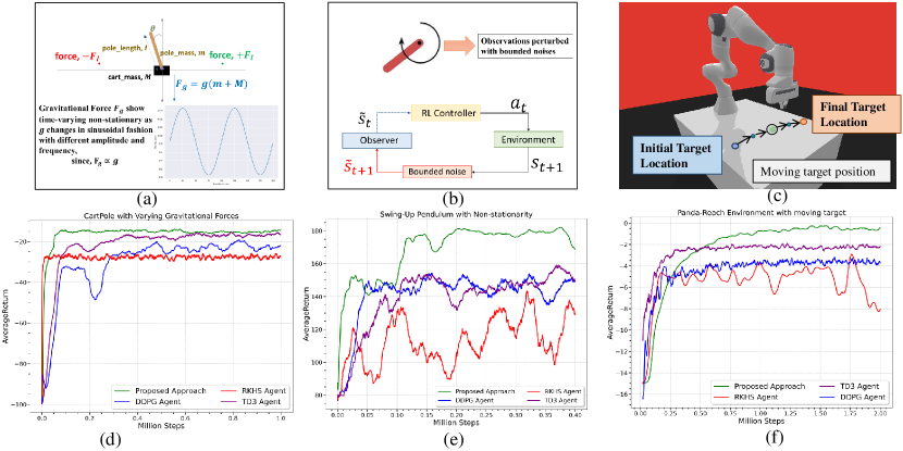
Figure 3: (a) NS Continuous CartPole environment, (b) NS Swing-up Pendulum Environment, (c) NS Reach Task, (d)-(e)-(f) learning curve comparison between proposed approach and baselines

IV-C Inner-product based Evaluation for Adaptive-H

RKHS possesses all properties of a Vector Space and we can compute the inner-product between consecutive policy gradients estimated through any trajectory $\xi_{k}$ sampled by current policy $\pi_{h_{k}}(\cdot|s_{i})$. The kernel matrix $\mathcal{K}(\cdot,\cdot)$ encodes the prior experiences with the covariance shift happened for underlying non-deterministic transition dynamics and $\mathcal{K}(\cdot,\cdot)$ can be regarded as a measure of proximity between different kernels in Hilbert Space in turn defining complex function space within which we can detect sequence of control policies for handling dynamic variance. This non-parametric representation of policy distributions grants an adaptive remolding of the old policy $\pi_{h_{k}}$ into more upgraded new policy for continual state-space evolution.

The principal essence of this work is the introduction of an inner-product based similarity checkpoint between gradient updates for setting adaptive period defined as $\texttt{H}^{\prime}$ in Fig.1. For reward maximization in RL setting, the gradients must follow an ascent direction in the solution space. By Eq. (3), policy gradients $\nabla_{h_{k}}J_{s_{0}}(h_{k},\cdot)|_{s_{i}}$ with respect to current policy mean functional $h_{k}$ for current trajectory $\xi_{k}$ can be easily measured. With consecutive policy gradient functionals, an inner product $\langle\nabla_{h_{k}}J_{s_{0}}(h_{k},\cdot)|_{s_{0}},\nabla_{h_{k}}J_{s_{0}}(h_{k},\cdot)|_{s_{i}}\rangle_{\mathcal{H}}$ can be calculated as both policy gradients belong to same RKHS. This inner product based similarity evaluation adjusts the confidence on current actions and adaptively sets the time-frame window $\texttt{H}^{\prime}$. Besides, after each optimal action execution, current snapshot of NS-MDP is recorded for gradient estimation. Since, the state transition function and reward distribution is continually evolving, parts of previously suggested actions $\{a_{i}\}_{i=0}^{n}$ from previous mapping $h_{k}$ will become sub-optimal and there emerges an appeal to relearn new mapping $h_{k+1}$ in between a full episodic interaction. Our proposed approach suggests that optimal point to prematurely upgrade to new policy. Theoretically, with respect to the underlying non-stationarity, $h_{k}$ will be outside of an $\epsilon$ neighborhood of the optimal solution i.e $|\nabla_{h_{k}}J_{s_{0}}(h_{k})|>\epsilon$. We need to update our policy and learn new action mapping functional $h_{k+1}$ whenever the policy gradients do not follow an ascent direction during optimization. Whenever, the condition $\langle\nabla_{h_{k}}J_{s_{0}}(h_{k},\cdot)|_{s_{0}},\nabla_{h_{k}}J_{s_{0}}(h_{k},\cdot)|_{s_{i}}\rangle_{\mathcal{H}}\geq Z\epsilon/2$ violates during finishing actions from old policy, the agent immediately retreats and do a revisit to policy upgrade for more updated actions. Mathematical proof of this statement is (inspired by [8]) shown as Theorem 1 in Appendix. We added the Appendix in https://sites.google.com/view/adaptiveh. We have discussed thoroughly and elaborately the mathematical validations of our proposed method in terms of RKHS. Moreover, this positive lower bound on the dot product based evaluation metric also turns the dynamic regret term $R_{k}$ into non-negative sub-martingale, assuring convergence of our proposed framework as $R_{k}:=J_{s_{0}}(h_{k}^{*})-J_{s_{0}}(h_{k})$— converges to its optimal value as $\mathbb{E}[R^{*}]=\lim_{k\rightarrow\infty}R_{k}$. This is defined as well in detail in Theorem 2 of Appendix. Thus, our proposed approach confirms a fixed-point solution for the non-stationary environments.

V Experimentation Platforms

Through experiments, we focused to validate our central finding that existing state-of-the-art parametric method, such as TD3 and DDPG struggle to contrive a perfect model of the environment perturbed with persistent non-stationarity, while stochastic policy distribution represented non-parametrically in a vector-valued RKHS can emerge as an efficient substitute for various benchmarks. Moreover, by launching frequent, but adaptive upgrades from current policy to new policy, our learning algorithm has ensured faster learning convergence and sample-efficiency.

Environments–We replicated non-stationarity by molding two classic control benchmark problem with continuous perturbation of physics parameters or by coupling observations with noises. Besides, we have also used a high dimensional simulated robotics environment based on Panda-Gym [24] where a 7 Degree of Freedoms (DoFs) Franka Emika Panda Arm has to execute optimal actions to reach continuously translating target position smoothly and swiftly. NS CartPole—The first environment is the classic problem called Cartpole where the agent need to balance a pole on a moving cart by applying torques on the cart. We constructed a continuous action-space variant of this environment based on the discrete one from OpenAI Gym[25]. We consider changes by continuously varying the magnitude, within bounds, of gravitational force, a physics parameter of the system as drawn in Fig.3(a), and the agent needs to dynamically adapt to this variation. NS InvertedPendulum—The second environment is the Swing-Up Pendulum environment. In this problem, we cluttered observation-space with bounded random noises to reproduce real-world latency and noise as shown in Fig.3(b). NS ReachTask—The last environment is based on a high-dimensional robotics environment where we introduced a real-world non-stationarity where the target location for a 7 DoFs robotic manipulator is continuously moving through a varying, but bounded, speed at a particular direction as shown in Fig.3 (c). Here, we assured that the target location always remains within the reachable workspace of the Panda Arm.

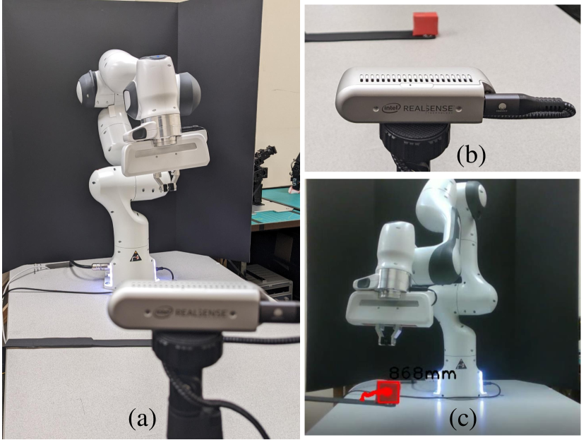
Figure 4: (a) Hardware setup with a 7 DOFs Franka Emika Panda Arm (b) Intel RealSense Depth Sensing Camera as tracking sensor to track the position of the moving target position(red colored box), (c) Position tracking through Depth Sensing Camera.

Real Hardware Setup– To validate our study in a real world scenario, we have mostly focused on the simulated robotic non-stationary environment to perform the real-hardware experimentation and we have used here the same 7-DoF Franka Emika Panda robot arm, that is mounted on table-top similar to simulation environment as shown in Fig.4(a). Besides, we have utilized here a Intel RealSense Depth Camera D435i for tracking the dynamically moving target location and extracting the depth information to obtain the current target position in 3D coordinate frame. This information is fed to RL controller as current 3D target location is a part of the state-space vector for our RKHS based learning algorithm. The Franka Arm integrated library–libfranka and Franka ROS turns the communication protocol between simulation and hardware very trouble-free through low-latency and low-noise communication based on ROS ecosystem.

VI Results Analysis

Our experiments seek to explore the following queries:

1. Does introducing kernel-centric stochastic policy learning in an RKHS deliberately showcase better performance than baselines in a non-stationary settings?

2. How much does the degree of non-stationary inference affect the performance of our AdaptiveH approach?

3. Does the proposed infinite-dimensional feature space initiate sequence of optimal policies at perfect interruption point for handling varying dynamics?

Better Learning Performance in Non-Stationary settings– The baselines to validate our proposed methodology are TD3 and DDPG implementation from OpenAI Baselines[26] and RKHS non-parametric policy gradient. Our evaluation criteria is the cumulative average return the agent gains on each trial. Learning curves are plotted in Fig. 3 (d)-(f) for three respective environments. From the learning curves drawn for environments, it is apparent that our proposed method promisingly outperformed all the baselines. Our method largely stabilizes the learning curves as episodic interaction increases, where the baseline DDPG exhibits relatively high variance in both NS CartPole and NS InvertedPendulum environments. Baseline agent–TD3 shows relatively better performance but it takes larger amount of training time to reach convergence in NS CartPole and in case of NS InvertedPendulum, TD3 agent lacks any promising performance due to uncontrolled stochastic perturbations. Moreover, the baseline RKHS method traps inside local minima, since it can not accomplish frequent policy update when required. Our method grants faster convergence and better sample-efficiency. In NS ReachTask, from the learning curve shown in Fig.3(f), it is apparent that our proposed approach has earned the maximum utility, while the baseline methods TD3 and DDPG stabilize but can not guarantee of achieving maximum rewards. Since, this is a high-dimensional environment, kernel based method required more training time to accumulate adequate amounts of experiences to build the kernel matrix and handle the dynamic shift through optimal action execution.

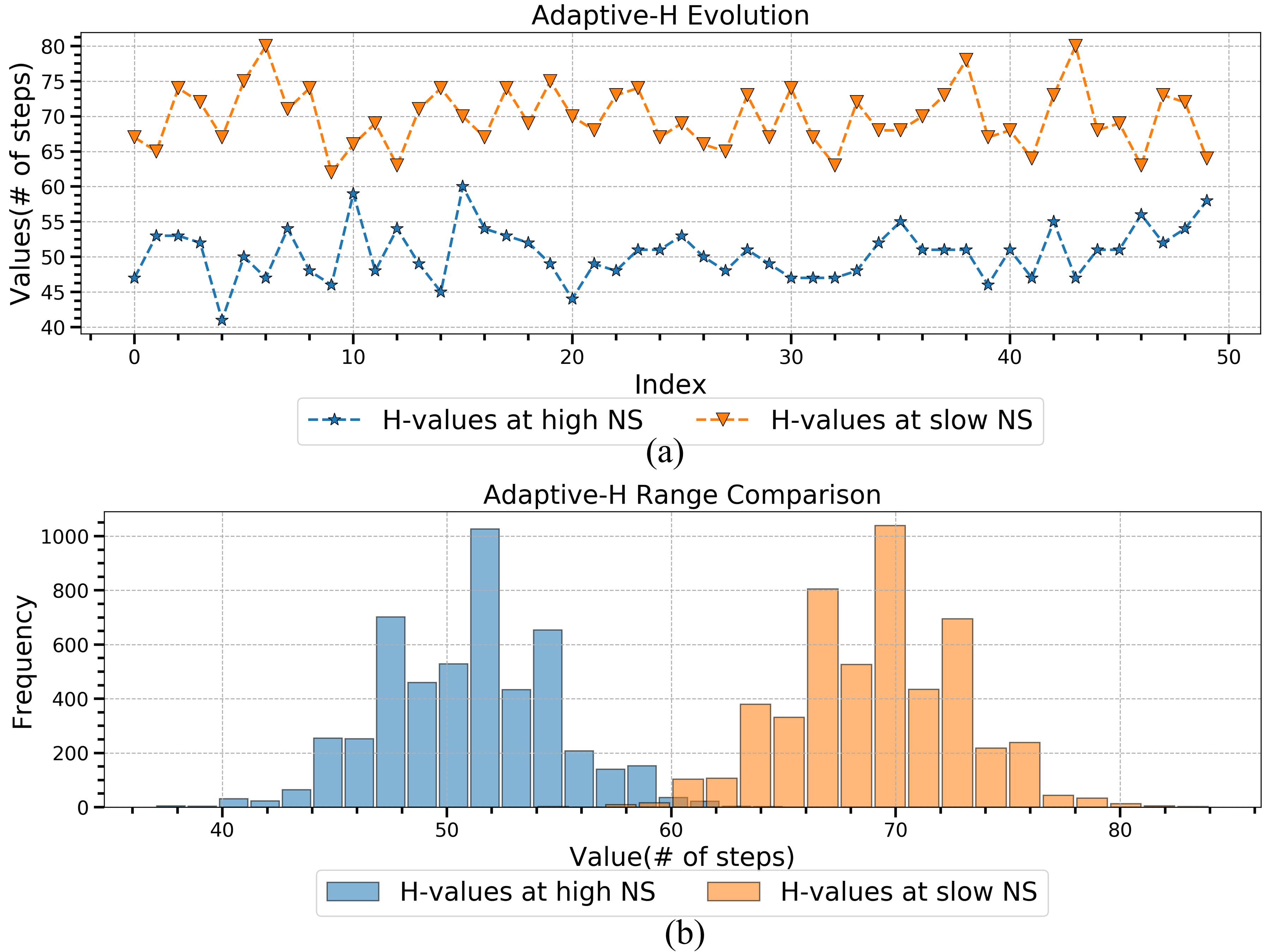
Figure 5: (a) Evolution of window-H of optimal actions for in Cart-Pole environment. (b) Comparison to differentiate range of H-values at two different non-stationary level.

Optimal Action Executions within AdaptiveH Window— Our proposed approach enables the learning agent to bisect the initial action sequence into two parts-optimal actions and outdated actions. The algorithm suggests the agent to upgrade its current action-mapping functional at the action interruption point and the updated policy samples more compatible actions to address the varying dynamics of the environment. We have experimented it in real-hardware setup using the Panda Arm. We have added sequence of snapshots of adaptive policy adjustment and action execution in Fig.7. We showcased that our robotic entity only executes the optimal part of action sequences to swiftly reach its dynamic target location and revisit the policy upgrade several times to handle the varying dynamics of moving target location.

Varying Degree of Non-stationarity— We also evaluated our method in NS CartPole with more high-frequency gravitational changes to authenticate whether the proposed approach can generalize to faster environmental shift. In Fig.5, we drew a comparison on how the adaptive window H varies with different magnitude of non-stationary shifts. As shown in Fig.5(a), when the environment possesses higher variance, then H values narrow down to lower values. Also, In Fig.5(b), it is very clear that for slower non-stationary benchmarks, periods of optimal actions are higher. Reasonably, when the transition dynamics is shifting very fast, but within bounds, policy upgrade is also required to be more frequent to maximize agent’s performance.

The learning curve for different non-stationarity has been shown in Fig. 6. From the figure, it is remarkably vivid that in a more complex non-stationary environment, our agent can function more optimally than both baselines. Although, the performance for the proposed approach while dealing with high stochasticity slightly worsens, it is totally interpretable that learning control-policies will be strategically strenuous considering high complexity. Besides, the baseline TD3 agent performs admirably better when the environment is perturbed with slower dynamic alterations. But still our proposed approach achieves faster convergence since the agent is empowered with additional dynamic adaptable ability in accordance to system variance.

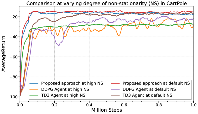
Figure 6: Comparison when degree of non-stationary is changed

VII Conclusion

Our adaptive non-parametric learning framework, through exploiting the inner-product similarity evaluation in RKHS, has outperformed the classic TD3 and DDPG for multiple standard benchmarks modified with dynamically varying transition probabilities and reward functions.

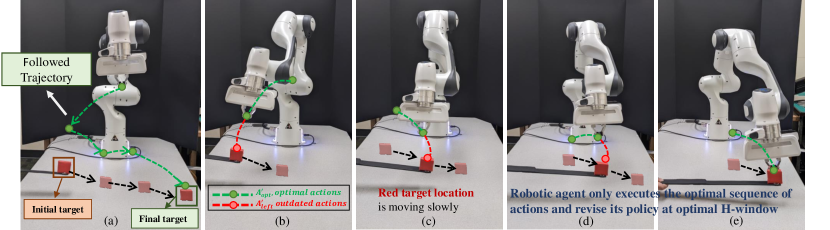
Figure 7: (a) Followed Adaptive Trajectory and dynamically varying target location, (b) only optimal part of action sequence executed and robot upgrades its policy at interruption point, (c)-(d) robot adaptively replans its trajectory to handle moving dynamics, (f) robotic agent swiftly reaching the target location

Maybe most importantly, our results have clearly demonstrated, both theoretically and empirically, the significant benefits of estimating self-adaptive window H in generating the sequence of optimal control policies that maximizes the utility values. In future research, we plan to investigate more complex robotic scenarios in dynamically challenging environments such as highly cluttered work space and stochastic sensor modality.

See pages - of complete.pdf

References

- [1] V. Mnih, K. Kavukcuoglu, D. Silver, A. Graves, I. Antonoglou, D. Wierstra, and M. Riedmiller, “Playing Atari with Deep Reinforcement Learning,” arXiv e-prints, p. arXiv:1312.5602, Dec. 2013.
- [2] J. Ibarz, J. Tan, C. Finn, M. Kalakrishnan, P. Pastor, and S. Levine, “How to train your robot with deep reinforcement learning: lessons we have learned,” The International Journal of Robotics Research, 2021. [Online]. Available: https://doi.org/10.1177/0278364920987859
- [3] T. P. Lillicrap, J. J. Hunt, A. Pritzel, N. Heess, T. Erez, Y. Tassa, D. Silver, and D. Wierstra, “Continuous control with deep reinforcement learning,” 4th International Conference on Learning Representations (ICLR 2016), 2016. [Online]. Available: http://arxiv.org/abs/1509.02971v6
- [4] S. Fujimoto, H. van Hoof, and D. Meger, “Addressing Function Approximation Error in Actor-Critic Methods,” arXiv e-prints, p. arXiv:1802.09477, Feb. 2018.
- [5] D. Silver, G. Lever, N. Heess, T. Degris, D. Wierstra, and M. Riedmiller, “Deterministic policy gradient algorithms,” in International conference on machine learning. PMLR, 2014, pp. 387–395.
- [6] S. Thrun, “Probabilistic algorithms in robotics,” AI Magazine, vol. 21, no. 4, p. 93, Dec. 2000. [Online]. Available: https://ojs.aaai.org/index.php/aimagazine/article/view/1534
- [7] G. Lever and R. Stafford, “Modelling Policies in MDPs in Reproducing Kernel Hilbert Space,” in Proceedings of the Eighteenth International Conference on Artificial Intelligence and Statistics, ser. Proceedings of Machine Learning Research, G. Lebanon and S. V. N. Vishwanathan, Eds., vol. 38. San Diego, California, USA: PMLR, 09–12 May 2015, pp. 590–598. [Online]. Available: http://proceedings.mlr.press/v38/lever15.html
- [8] S. Paternain, J. A. Bazerque, and A. Ribeiro, Policy Gradient for Continuing Tasks in Non-stationary Markov Decision Processes, 2020. [Online]. Available: https://arxiv.org/abs/2010.08443
- [9] E. Lecarpentier and E. Rachelson, “Non-Stationary Markov Decision Processes, a Worst-Case Approach using Model-Based Reinforcement Learning, Extended version,” arXiv e-prints, p. arXiv:1904.10090, Apr. 2019.
- [10] G. R. G. Lanckriet, N. Cristianini, P. Bartlett, L. El Ghaoui, and M. I. Jordan, “Learning the kernel matrix with semi-definite programming,” USA, Tech. Rep., 2002.
- [11] S. Padakandla, P. K. J., and S. Bhatnagar, “Reinforcement learning algorithm for non-stationary environments,” Applied Intelligence, vol. 50, no. 11, pp. 3590–3606, June 2020. [Online]. Available: https://doi.org/10.1007/s10489-020-01758-5
- [12] N. Singh, P. Dayama, V. Pandit, et al., “Change point detection for compositional multivariate data,” arXiv preprint arXiv:1901.04935, 2019.
- [13] A. Xie, J. Harrison, and C. Finn, “Deep reinforcement learning amidst continual structured non-stationarity,” in Proceedings of the 38th International Conference on Machine Learning, ser. Proceedings of Machine Learning Research, M. Meila and T. Zhang, Eds., vol. 139. PMLR, 18–24 Jul 2021, pp. 11 393–11 403. [Online]. Available: https://proceedings.mlr.press/v139/xie21c.html
- [14] S. Paternain, J. A. Bazerque, and A. Ribeiro, Stochastic policy gradient ascent in reproducing kernel hilbert spaces. Transactions on Automatic Control, 2021, vol. 66. [Online]. Available: https://arxiv.org/abs/2010.08443
- [15] Y. Chandak, G. Theocharous, S. Shankar, M. White, S. Mahadevan, and P. Thomas, “Optimizing for the future in non-stationary MDPs,” in Proceedings of the 37th International Conference on Machine Learning, ser. Proceedings of Machine Learning Research, H. D. III and A. Singh, Eds., vol. 119. PMLR, 13–18 Jul 2020, pp. 1414–1425. [Online]. Available: https://proceedings.mlr.press/v119/chandak20a.html
- [16] W. C. Cheung, D. Simchi-Levi, and R. Zhu, “Reinforcement learning for non-stationary Markov decision processes: The blessing of (More) optimism,” in Proceedings of the 37th International Conference on Machine Learning, ser. Proceedings of Machine Learning Research, H. D. III and A. Singh, Eds., vol. 119. PMLR, 13–18 Jul 2020, pp. 1843–1854. [Online]. Available: https://proceedings.mlr.press/v119/cheung20a.html
- [17] B. C. da Silva, E. W. Basso, A. L. C. Bazzan, and P. M. Engel, “Dealing with non-stationary environments using context detection,” in Proceedings of the 23rd International Conference on Machine Learning, ser. ICML ’06. New York, NY, USA: Association for Computing Machinery, 2006, p. 217–224. [Online]. Available: https://doi.org/10.1145/1143844.1143872
- [18] M. L. Puterman, Markov Decision Processes: Discrete Stochastic Dynamic Programming, 1st ed. USA: John Wiley & amp; Sons, Inc., 1994.
- [19] Y. Engel and M. Ghavamzadeh, “Bayesian policy gradient algorithms,” Advances in NIPS, vol. 19, p. 457, 2007.
- [20] T. Xiao, E. Jang, D. Kalashnikov, S. Levine, J. Ibarz, K. Hausman, and A. Herzog, “Thinking while moving: Deep reinforcement learning with concurrent control,” arXiv preprint arXiv:2004.06089, 2020.
- [21] P. M. J. . T. C. Tuyen Pham Le, Vien Anh Ngo, “Importance sampling policy gradient algorithms in reproducing kernel hilbert space,” The Artificial Intelligence Review, vol. 52, pp. 2039–2059, 2019. [Online]. Available: https://doi.org/10.1007/s10462-017-9579-x
- [22] X. Xu, D. Hu, and X. Lu, “Kernel-based least squares policy iteration for reinforcement learning,” IEEE transactions on neural networks, vol. 18, no. 4, pp. 973–992, 2007.
- [23] J. A. Boyan, “Least-squares temporal difference learning,” in ICML, 1999, pp. 49–56.
- [24] Q. Gallouédec, N. Cazin, E. Dellandréa, and L. Chen, “panda-gym: Open-Source Goal-Conditioned Environments for Robotic Learning,” 4th Robot Learning Workshop: Self-Supervised and Lifelong Learning at NeurIPS, 2021.
- [25] G. Brockman, V. Cheung, L. Pettersson, J. Schneider, J. Schulman, J. Tang, and W. Zaremba, “Openai gym,” arXiv preprint arXiv:1606.01540, 2016.
- [26] A. Raffin, A. Hill, A. Gleave, A. Kanervisto, M. Ernestus, and N. Dormann, “Stable-baselines3: Reliable reinforcement learning implementations,” Journal of Machine Learning Research, vol. 22, no. 268, pp. 1–8, 2021. [Online]. Available: http://jmlr.org/papers/v22/20-1364.html