LOCAT: Low-Overhead Online Configuration Auto-Tuning of Spark SQL Applications

Abstract.

Spark SQL has been widely deployed in industry but it is challenging to tune its performance. Recent studies try to employ machine learning (ML) to solve this problem. They however suffer from two drawbacks. First, it takes a long time (high overhead) to collect training samples. Second, the optimal configuration for one input data size of the same application might not be optimal for others.

To address these issues, we propose a novel Bayesian Optimization (BO) based approach named LOCAT to automatically tune the configurations of Spark SQL applications online. LOCAT innovates three techniques. The first technique, named QCSA, eliminates the configuration-insensitive queries by Query Configuration Sensitivity Analysis (QCSA) when collecting training samples. The second technique, dubbed DAGP, is a Datasize-Aware Gaussian Process (DAGP) which models the performance of an application as a distribution of functions of configuration parameters as well as input data size. The third technique, called IICP, Identifies Important Configuration Parameters (IICP) with respect to performance and only tunes the important parameters. As such, LOCAT can tune the configurations of a Spark SQL application with low overhead and adapt to different input data sizes.

We employ Spark SQL applications from benchmark suites $TPC-DS$, $TPC-H$, and $HiBench$ running on two significantly different clusters, a four-node ARM cluster and an eight-node x86 cluster, to evaluate LOCAT. The experimental results on the ARM cluster show that LOCAT accelerates the optimization procedures of Tuneful (Fekry et al., 2020), DAC (Yu et al., 2018), GBO-RL (Kunjir and Babu, 2020), and QTune (Li et al., 2018) by factors of $6.4\times$, $7.0\times$, $4.1\times$, and $9.7\times$ on average, respectively. On the x86 cluster, LOCAT reduces the optimization time of Tuneful, DAC, GBO-RL, and QTune by factors of $6.4\times$, $6.3\times$, $4.0\times$, and $9.2\times$ on average, respectively. Moreover, LOCAT improves the performance of the applications on the ARM cluster tuned by Tuneful, DAC, GBO-RL, and QTune by factors of $2.4\times$, $2.2\times$, $2.0\times$, and $1.9\times$ on average, respectively. On the x86 cluster, LOCAT improves the performance of these applications tuned by Tuneful, DAC, GBO-RL, and QTune by factors of $2.8\times$, $2.6\times$, $2.3\times$, and $2.1\times$ on average, respectively.

1. Introduction

Big data query systems such as Hive (Thusoo et al., 2009), Presto (Sethi et al., 2019), and Spark SQL (Armbrust et al., 2015) have been widely deployed in industry to mine valued information from massive data efficiently (Rida, 2020). As a higher level library on top of Apache Spark (Zaharia et al., 2010), Spark SQL not only inherits Spark’s excellent big data processing capabilities, but also provides support for query-like large-scale data analysis, such as OnLine Analytical Processing (OLAP) (Lv et al., 2015; Cuzzocrea, 2015).

However, it is challenging to tune the configuration parameters of a Spark SQL application for optimal performance because of two reasons. First, the lower layer Spark and the upper layer Spark SQL both have a number (e.g.,$>20$) of configuration parameters. Not only the ones for Spark SQL (e.g., spark.sql.shuffle.partitions) itself, but also those for Spark (e.g., spark.executor.memory) significantly affect the performance of a Spark SQL application. For example, the parameter spark.executor.memory specifies the amount of memory used by an executor process (SparkConf, 2022). Too large value of it may cause a long garbage collection time (Chiba and Onodera, 2016) pausing the application whereas too small value may even lead to out of memory (OOM) errors (Kunjir and Babu, 2020). Therefore, tuning the larger number of parameters for optimal performance of a Spark SQL application is difficult. Second, the configuration parameters within the same layer as well as from different layers may intertwine with each other in a complex way with respect to performance, further troubling the performance tuning of a Spark SQL application.

Recent studies propose to leverage machine learning (ML) to tune the configurations for Spark programs (Yu et al., 2018; Kunjir and Babu, 2020) and database systems (Li et al., 2018; Zhang et al., 2019). However, current ML-based approaches have two drawbacks. First, these approaches take a long time to collect training samples, which is inconvenient in practice. The long time stems from four factors. (1) The number of training samples is large (e.g., 1000 — 10000), which is the nature of ML-based approaches. (2) The time used to collect each training sample of an application is typically long (e.g., several minutes) because it is collected by running the application on a real cluster with a random configuration. (3) A Spark SQL application typically consists of a number (e.g., 20) of queries. The more queries in a Spark SQL application generally make it take longer time to execute and in turn longer time to collect one training sample. (4) ML-based approaches generally need more training samples when tuning more parameters.

Second, most ML-based approaches can not adapt to the changes of input data sizes of a Spark SQL application. That is, a configuration making a Spark SQL application achieve the optimal performance for one input data size might not produce optimal performance for another input data size. This makes the same application need to be re-tuned when its input data size is changed, which is time-consuming. However, customers typically do not change their Spark SQL applications frequently while definitely change the input data size of the same application.

To address these issues, we propose a novel approach dubbed LOCAT to automatically tune the configurations of a Spark SQL application online. LOCAT’s first key innovation is that we observe an important as well as interesting finding: different queries in a Spark SQL application respond to configuration parameter tuning with significantly different sensitivity. Some queries of an application are insensitive to the parameter tuning at all, and we therefore call them configuration-insensitive queries. Based on this finding, we remove the configuration-insensitive queries from a Spark SQL application when we run the application with random configurations to collect training samples. As such, the sample collection time can be dramatically reduced.

Figure 1. An Overview of the Spark SQL framework.

The second key innovation is that we propose a Datasize-Aware Gaussian Process (DAGP) to take the input data size in addition to the configuration parameters of a Spark SQL application into consideration as tuning the configuration parameters. In contrast, other Gaussian Process (GP) based approaches such as CherryPick (Alipourfard et al., 2017) only consider the configuration parameters, which needs to perform the time-consuming parameter re-tuning when an application’s input data size is changed. The third innovation is that we propose to identify the important configuration parameters of a Spark SQL application and in turn only tune them in BO (Bayesian Optimization) iterations. We name this technique IICP. Generally, tuning more parameters takes more iterations to find the optimal configuration for an application by BO. IICP therefore takes less iterations and in turn shorter time to find the optimal configuration.

In particular, this paper makes the following contributions.

• We find that some queries of a Spark SQL application are insensitive to configuration parameter tuning with respect to performance by Query Configuration Sensitivity Analysis (QCSA).

• We propose to leverage Gaussian Process (GP) to model the relationship between performance and the input data size of a Spark SQL application in addition to the configuration parameters. As such, our approach can adapt to different input data sizes of the same application and we name this technique DAGP (Datasize-Aware Gaussian Process).

• We propose to identify the important configuration parameters (IICP) of a Spark SQL application and only tune these parameters in order to reduce the tuning time.

• By putting it all together, we develop an online configuration parameter tuning approach for Spark SQL applications with low overhead, named LOCAT.

• We employ Spark SQL applications from benchmark suites $TPC-DS$, $TPC-H$, and $HiBench$ running on two different clusters — a four-node ARM cluster and an eight-node x86 cluster — to evaluate LOCAT. The results on the ARM cluster show that LOCAT accelerates the optimization procedures of Tuneful (Fekry et al., 2020), DAC (Yu et al., 2018), GBO-RL (Kunjir and Babu, 2020), and QTune (Li et al., 2018) by factors of $6.4\times$, $7.0\times$, $4.1\times$, and $9.7\times$ on average, respectively. On the x86 cluster, LOCAT reduces the optimization time used by Tuneful, DAC, GBO-RL, and QTune by factors of $6.4\times$, $6.3\times$, $4.0\times$, and $9.2\times$ on average, respectively. Moreover, LOCAT improves the applications’ performance on the ARM cluster tuned by Tuneful, DAC, GBO-RL, and QTune by factors of $2.4\times$, $2.2\times$, $2.0\times$, and $1.9\times$ on average, respectively. On the x86 cluster, LOCAT improves the applications’ performance tuned by Tuneful, DAC, GBO-RL, and QTune by factors of $2.8\times$, $2.6\times$, $2.3\times$, and $2.1\times$ on average, respectively.

The rest of this paper is organized as follows. Section 2 introduces the background and motivation. Section 3 presents our LOCAT approach. Section 4 describes the experimental setup. Section 5 provides and analyzes the experimental results. Section 6 describes the related work and Section 7 concludes the paper.

2. Background and Motivation

2.1. Spark SQL Framework

Spark SQL (Armbrust et al., 2015) is built on top of Apache Spark (Zaharia et al., 2010) to facilitate high-performance structured data processing. Unlike Spark RDD APIs, Spark SQL interfaces provide Spark with more information about the structure of both data and computation being performed (Armbrust et al., 2015). It is therefore widely used in industry (Baldacci and Golfarelli, 2019) such as OLAP (Lv et al., 2015). As shown in Figure 1, a Spark SQL application typically consists of a number of queries. The Spark SQL framework transforms each query into a DAG (directed acyclic graph) which is then split into a collection of stages consisting of a set of parallel tasks. Each task corresponds to a partition (P in Figure 1) computing partial results of an application. Each stage may depend on other stages, called lineage stored in a RDD.

The DAG scheduler of Spark schedules the tasks on several executors to execute in parallel. This parallelism is controlled by several configuration parameters. For example, in Yarn (Vavilapalli et al., 2013) mode, the parameter spark.executor.instances specifies the number of executors, and spark.executor.cores specifies the number of cores used by each executor. The product of the number of executors and the number of cores per executor determines the maximum number of total tasks that can be executed by a Spark SQL cluster at a time.

In summary, the performance of a Spark SQL application is controlled by more than 200 configuration parameters, which can be generally classified into two levels: the Spark SQL configuration parameters (upper level) and the Spark core ones (lower level). The upper level parameters specify the properties of a Spark SQL application. For example, spark.sql.autoBroadcastJoinThreshold specifies the maximum size in bytes for a table that is broadcasted to all workers when performing a join operation, which significantly affects its performance. The lower level parameters specify fourteen aspects of the Spark core such as execution parallelism and memory management. For instance, the above mentioned spark.executor.cores and spark.executor.instances control the computing parallelism, and dramatically influence the performance of a Spark SQL application too. Moreover, the upper level configurations may interact with the lower level ones in a complex way, which makes tuning configurations for a Spark SQL application extremely difficult.

2.2. Bayesian Optimization

Bayesian Optimization (BO) (Mockus, 2012) is a principled technique based on Bayes Theorem to direct an efficient and effective search of a global optimization problem. It minimizes or maximizes an objective function f iteratively through adaptive sampling of the search space with a manner that balances exploration and exploitation. BO has two key components: surrogate model and acquisition function. The surrogate model is used to model the objective function f and the acquisition function guides the selection of the next evaluation sample. BO iteratively fits the surrogate model by using the samples selected by the acquisition function and finally finds the minimal/maximal objective function f.

The surrogate models can be other machine learning models such as Random Forest (RF) and Boosted Regression Trees (BRT) that have a good ability to model the non-linear interactions (Hsu et al., 2018). However, they are weak in theoretical guarantees on the confidence bounds while GP (Gaussian Process) isn’t (Kunjir and Babu, 2020). Moreover, GP has many outstanding features such as supporting for noisy observations and gradient-based methods (Shahriari et al., 2015). We therefore apply GP (Rasmussen, 2004; Williams and Barber, 1998) as the surrogate model of BO in this work.

As for acquisition functions, the popular ones are expected improvement (EI) (Jones et al., 1998), probability of improvement (PI) (Hoffman et al., 2011), and GP upper confidence bound (GP-UCB) (Rasmussen, 2004). Among which, EI is one of the most widely used acquisition functions. However, we do not directly use EI. Instead, we leverage the EI with Markov Chain Monte Carlo (EI-MCMC) (Snoek et al., 2012) for better overall performance, which has shown better performance compared to other acquisition functions across a wide range of test cases (Snoek et al., 2012).

2.3. Motivation

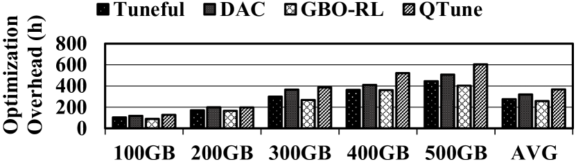
Figure 2. The time used to find the optimal configuration of $TPC-DS$ by Tuneful, DAC, GBO-RL, and QTune.

Although the time (e.g., seconds or minutes) used to execute a Spark SQL application is shorter than that (e.g., hours or days) used to optimize its execution, it is still necessary to optimize it because the optimization is a one-shot task while application is repeatedly executed many times in a long time such as months or years. Saving a short time in each execution would accumulate a long time, which is a large benefit. To optimize Spark SQL applications, the easiest way is to employ the state-of-the-art (SOTA) approaches. However, we find that these approaches all take a long time (e.g., days or weeks) to find the optimal configuration. Figure 2 shows the time used by four SOTA approaches (Tuneful, GBO-RL, DAC for Spark applications, and QTune for database systems) to find the optimal configuration for $TPC-DS$. We made two observations. For one, the time used by these approaches is at least 89 hours (GBO-RL) when the input data size of $TPC-DS$ is 100 GB. Second, the time used by all the approaches is getting significantly longer when the input data size becomes larger.

In industry, the input data size of a Spark SQL application is typically from hundreds of Giga bytes to Tera bytes, even Peta bytes (Rida, 2020). In such a case, it is very inconvenient, if feasible, to apply the above approaches to find the optimal configurations for Spark SQL applications. For example, we optimize $TPC-DS$ with 500 GB of data by using GBO-RL on our ARM cluster, it took 402 hours (16.75 days)! This motivates this work.

3. LOCAT Approach

3.1. Overview

LOCAT is a configuration auto-tuning approach that automatically finds the optimal values of configuration parameters for an application running on a given cluster in a short time. It is designed for a common industrial usage: a Spark SQL application repeatedly runs many times with the size of input data changing over time.

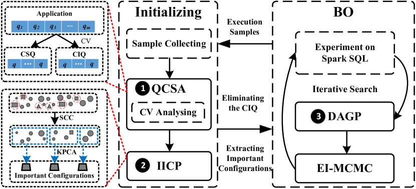
Figure 3. An Overview of LOCAT. BO — Bayesian Optimization. QCSA — Query Configuration Sensitivity Analysis. IICP — Identifying Important Configuration Parameters. DAGP — Data size Aware Gaussian Process. EI-MCMC — Expected Improvement with Markov Chain Monte Carlo.

Figure 3 shows the block diagram of LOCAT. As can be seen, it consists of three components: query configuration sensitive analysis (QCSA), identifying important configuration parameters (IICP), and data-size aware Gaussian Process (DAGP). QCSA analyzes how the performance (e.g., latency) of each query of a Spark SQL application varies when the configuration parameter values change. If the performance of a query varies significantly when parameter values change, we call it configuration sensitive query. Otherwise, we call it configuration insensitive query. IICP identifies the important parameters for a Spark SQL application to be tuned. DAGP models the performance of a Spark SQL application as a Gaussian Process (GP) of the input data size of the application in addition to the configuration parameters.

When we employ LOCAT to optimize the configurations of a Spark SQL application, we firstly leverage QCSA to identify the configuration insensitive queries of the application and in turn remove these queries. We call the resulted application RQA (reduced query application). Subsequently, we use the component IICP to select the important configuration parameters to tune for the RQA. Finally, the selected configuration parameters and the input data size of the RQA are input to the DAGP which is used as the surrogate model of BO to search for the optimal configuration of the RQA. Note that the optimal configuration of the original Spark SQL application is the same as that of the RQA.

3.2. Query Configuration Sensitivity Analysis

As aforementioned, ML-based configuration auto-tuning needs to collect a large number of training samples for an application by running the application on a real cluster the same number of times, which is time-consuming. One possible way to reduce the time is to shorten the execution time of each run. Since a Spark SQL application consists of a number of queries, the execution time of the application would be shortened if some queries can be removed from it. The performance of the removed queries should not be influenced by the value variance of the configuration parameters. Moreover, removing queries should not affect the performance of other queries either. However, we do not know which queries of an application can be removed as collecting training samples for it.

To address this issue, we propose query configuration sensitivity analysis (QCSA) to identify which queries can be removed. Figure 4 shows the block diagram of QCSA. As can be seen, the Spark SQL application $AppA$ executes on a given cluster $N_{QCSA}$ times through BO with DAGP, each with a different configuration. A configuration can be represented by a vector as follows.

(1) $$conf=\{c_{1},c_{2},...,c_{p},...,c_{k}\}$$

with $c_{p}$ the $p^{th}$ configuration parameter value and $k$ the total number of configuration parameters. A random configuration is generated by randomly setting the $p^{th}$ value of $conf$ within the $p^{th}$ parameter’s value range and $p$ can be any value between 1 and $k$. In $AppA$’s each execution, QCSA records each query’s execution time. It is represented by $t_{q_{ij}}$ where $q_{ij}$ denotes the $i^{th}$ query of the $j^{th}$ execution of the $AppA$. After the $AppA$ executes $N_{QCSA}$ times, we have collected a matrix $S$ denoted as follows

(2) $$S=\{t_{q_{ij}}\},i=1,2,...,m;j=1,2,...,N_{QCSA}$$

with $m$ the number of queries in $AppA$.

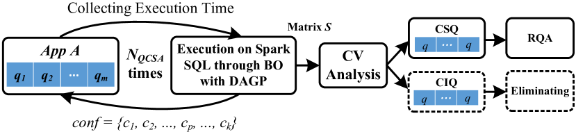
Figure 4. The QCSA diagram. DAGP — Data size Aware Gaussian Process. CV — Coefficient of Variation. RQA — Reduced Query Application. CSQ — Configuration Sensitive Query. CIQ — Configuration Insensitive Query.

We employ Coefficient of Variation (CV), also known as standard deviation divided by mean, to represent the configuration sensitivity of a query $q_{i}$ because CV is a standard measure of dispersion of a probability distribution or frequency distribution. As such, query $q_{i}$’s configuration sensitivity is calculated by equation (3).

(3) $$CV_{q_{i}}=\frac{1}{\bar{t_{q_{i}}}}\sqrt{\frac{1}{N_{QCSA}}\sum_{j=1}^{N_{QCSA}}(t_{q_{ij}}-\bar{t_{q_{i}}})^{2}}$$

with $CV_{q_{i}}$ the configuration sensitivity of query $q_{i}$, $\bar{t_{q_{i}}}$ the average execution time of query $q_{i}$, $N_{QCSA}$ the total number of executions of the $AppA$ with random configurations, and $t_{q_{ij}}$ the execution time of query $q_{i}$ in its $j^{th}$ execution. Note that there are $N_{QCSA}$ different $t_{q_{i}}$ s for $AppA$.

In general, higher $CV_{q_{i}}$ indicates the corresponding query $q_{i}$ of a Spark SQL application is more sensitive to configuration tuning. To remove some queries from a Spark SQL application when we collect training samples, we need to determine a suitable threshold of $CV$. However, it is difficult to set a absolute threshold such as $1$ for $CV$ because the value ranges of $CV$ for different queries of the same Spark SQL application might be significantly different, let alone different applications. We therefore need a relative way to determine the threshold for $CV$. It’s been proved that classifying $CV$ into high, medium and low is good enough (Lorenzo et al., 2015; Vaz et al., 2017) to leverage $CV$. We therefore equally divide the value range of a $CV$ into three non-overlapped partitions, as shown in equation (4).

(4) $$Width_{CV}=(max(CV_{q_{i}})-min(CV_{q_{i}}))/3$$

where $Width_{CV}$ is the width of each partition, and $max(CV_{q_{i}})$ as well as $min(CV_{q_{i}})$ are the maximum CV and minimum CV of query $q_{i}$ occurred in the $N_{QCSA}$ executions of application $AppA$, respectively. We classify a query with its $CV\in[0,min(CV_{q_{i}})+Width_{CV})$ as a configuration insensitive query (CIQ). Otherwise, the query is a configuration sensitive query (CSQ). To collect training samples for $AppA$, we first remove the CIQs and only remain the CSQs, making $AppA$ the reduced query application (RQA). Subsequently, we run the RQA a number of times, each with a random configuration. With the same configuration, the execution time of RQA is significantly shorter than that of the original $AppA$. As such, we can collect the same number of training samples as that needed to tune the configuration of the original $AppA$ but with dramatically shorter time.

3.3. Identifying Important Parameters

As mentioned in Section 1, another way to reduce the optimization time needed by ML-based approaches is to reduce the number of training samples by decreasing the number of parameters needing to be tuned. This is because ML-based approaches typically need to construct highly accurate performance models as functions of parameters. For the same accuracy, more training samples are needed to train a performance model if the model takes more parameters as input. We therefore propose to firstly identify the important configuration parameters (IICP) with respect to performance, and subsequently only select the important ones to build performance models. As such, the number of training samples needed to build high accuracy models can be reduced. Figure 5 shows that IICP consists of two stages: sample collection and IICP.

3.3.1. The sample collection stage

It collects the execution times of a small number of executions of a $AppA$ with a certain input data size, each execution with a random configuration. The execution times and configurations are stored in a matrix $S^{\prime}$ shown as:

(5) $$S^{\prime}=\{t_{i},conf_{i},ds\},i=1,2,...,N_{IICP}$$

with $t_{i}$ the execution time of $AppA$ with data size $ds$ executed with $conf_{i}$ defined by equation (1), and $N_{IICP}$ the number of executions of $AppA$. Smaller $N_{IICP}$ is better because we want to reduce the optimization time.

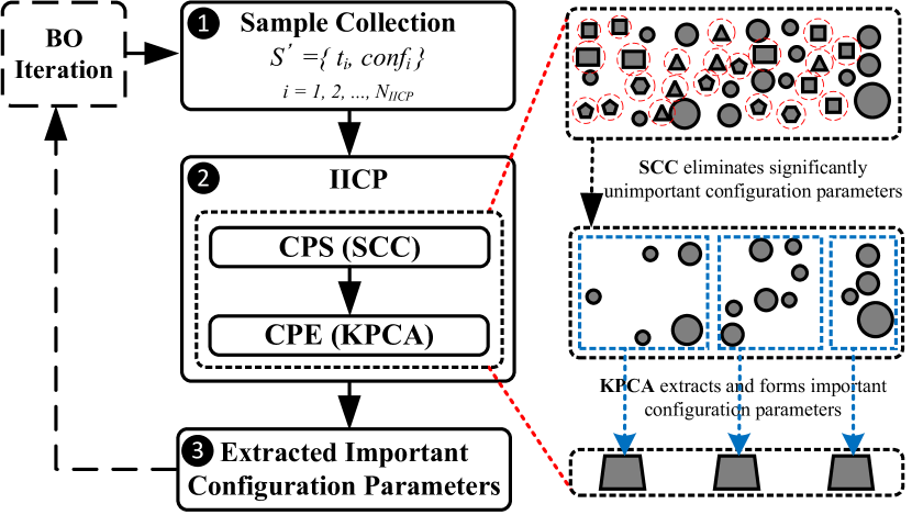
Figure 5. The block diagram of IICP. CPS — Configuration Parameter Selection. SCC — Spearman Correlation Coefficient. CPE — Configuration Parameter Extraction. KPCA — Kernel Principle Component Analysis.

3.3.2. The IICP stage

This stage extracts the important configuration parameters in terms of performance based on the samples collected by the sample collection stage. There are a lot of approaches such as metric quantification (Lv et al., 2018), feature selection (Chandrashekar and Sahin, 2014), feature extraction (Guyon et al., 2008) can be used to perform IICP. We do not employ the metric quantification approach used in (Lv et al., 2018) because it needs a large number of training samples, which is conflict with our goal. We do not use feature selection and extraction directly in this study either. Instead, we employ a novel hybrid approach which combines the feature selection and feature extraction.

We therefore employ two steps: configuration parameter selection (CPS) and configuration parameter extraction (CPE) which seem similar but significantly different. CPS removes the unimportant parameters from the vector $conf$ defined by equation (1) and the remaining ones form a new vector shown in equation (6).

(6) $$r\_conf=\{c_{1},c_{2},...,c_{i},...,c_{rk}\}$$

with $c_{i}$ the $i^{th}$ configuration parameter and $rk$ the number of remaining parameters after CPS is performed. Note that $rk$ is less than $k$. CPE further extracts important parameters from vector $r\_conf$. Note that these parameters are not the original configuration parameters. Instead, they are new parameters which are functions such as linear regressions of the original ones. These small number of new parameters are used to construct the DAGP of BO in this study. After BO converges, we derive the values of the original configuration parameters from the new parameters to optimally configure a Spark SQL application $AppA$. As such, the time used to search the optimal configuration for $AppA$ can be significantly reduced further.

CPS is implemented by using Spearman Correlation Coefficient (SCC) (Zar, 2005) which is a popular filter approach for feature selection (Zebari et al., 2020). SCC is an efficient multivariate analysis technique without learning involved to measure the strength of association between features (Cheng et al., 2021). Compared to Pearson Correlation Coefficient (PCC) (Bolboaca and Jäntschi, 2006), SCC is more suitable for IICP because the values of configuration parameters tuned in this study are discrete numerical variables. We calculate the SCC between each configuration parameter $c_{p}$ and the execution time $t_{i}$, and in turn eliminate $c_{p}$ if the absolute value of its corresponding SCC is less than $0.2$ (Zar, 2005), which is a common boundary value of SCC to identify poor correlation (Akoglu, 2018; Bhattacharyya et al., 1979). The remaining parameters are stored in $r\_conf$ which is defined by equation (6). However, the configuration parameters in $r\_conf$ may correlate with each other in a non-linear manner. This indicates that the size of $r\_conf$ can be further reduced but it can not be done by using SCC. We therefore design CPE based on the $r\_conf$ produced by CPS.

Our CPE is performed by Kernel Principal Component Analysis (KPCA) which is a powerful nonlinear feature extractor (Zhang and Yang, 2016). The common approach for feature extraction is Principle Component Analysis (PCA). PCA reduces the feature dimension by calculating the eigen vectors of a Covariance matrix of the original inputs. However, PCA can not extract the non-linear information from the original configuration space (Mika et al., 1998). KPCA extends PCA to make it be able to extract non-linear information by leveraging the kernel method. The crucial problem of KPCA is to select a suitable kernel and we select it by experiments. If we use the configuration parameters selected by KPCA with different kernels to configure a Spark SQL application to execute a number of times, the larger standard deviation (SD) of the execution times caused by a kernel indicates that the configuration parameters selected by the kernel are more important to execution time than those selected by other kernels.

We evaluate three mainstream kernel methods: Gaussian kernel, perceptron kernel, and polynomial kernel (Hao et al., 2013) in our experimental environment (Section 4) for two Spark SQL applications: $TPC-DS$ and $TPC-H$. As shown in Figure 6, the SDs of execution times caused by the Gaussian kernel are the largest for both $TPC-DS$ and $TPC-H$. This indicates that the configuration parameters selected by KPCA with the Gaussian kernel are more important than those selected with other kernels in terms of performance. We therefore choose Gaussian kernel in this study.

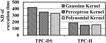
Figure 6. Kernel comparison. S.D — standard deviation.

3.4. Datasize-Aware Bayesian Optimization

Previous BO-based configuration optimization approaches such as CherryPick (Alipourfard et al., 2017) can not adapt to the input data size changes of an application. These approaches therefore can not be used online. To address this issue, we design Datasize-Aware Gaussian Process (DAGP) for BO to make it be able to adapt to data size changes.

In detail, we employ GP to model the execution time of a Spark SQL application with a certain configuration as a function of configuration parameters and input data size as follows.

(7) $$t=f(conf,ds)$$

with $t$ the execution time of a Spark SQL application, $conf$ the configuration vector defined by equation (1) used to configure the application, and $ds$ the input data size. As such, LOCAT can adapt to the data size changes of a Spark SQL application during optimization. We express the vector $\{conf,ds\}$ as $X_{e}$.

We now elaborate the function $f$ by Gaussian distribution (Rasmussen, 2004) as equation (8).

(8) $$f(X_{e})\sim GP(0,K(X_{E},X^{\prime}_{E}))$$

where $K$, the kernel function, denotes a covariance matrix. After we run a Spark SQL application with $n$ configurations with different input data sizes, we get a matrix $(X_{E},T)$ with $n$ $X_{e}$ and corresponding $t$ as input training set of GP. The $(X_{E},T)$ can be expressed by ($\{X_{e1},X_{e2},...,X_{en}\}$,$\{t_{1},t_{2},...,t_{n}\}$). $X^{\prime}_{E}$ and $X_{E}$ are two matrices of the same size. We solve the regression model posterior under Gaussian process prior and normal likelihood: $p[f(X_{e})|f(X_{e1}),f(X_{e2}),...,$ $f(X_{en}))]$ to get the joint probability distribution of $t$, the actual output value of the training sample, and $f_{*}$, the predicted value of a sample, as equation (9).

(9) $$\begin{bmatrix}t\\ f_{*}\end{bmatrix}=N\begin{bmatrix}0,\begin{bmatrix}K(X_{E},X_{E})+{{\delta_{n}}^{2}}I&K(X_{E},{X_{E}}_{*})\\ K(X_{E},X_{E})&K({X_{E}}_{*},{X_{E}}_{*})\end{bmatrix}\\ \end{bmatrix}$$

where ${X_{E}}_{*}$ is a set of samples to be predicted. $I$ is a $n$ dimensional identity matrix. ${\delta_{n}}^{2}$ is the variance of noise.

Next, we take the edge distribution of $f_{*}$ for the joint probability distribution expressed by equation (9), and the regression prediction form of the DAGP can be obtained from the edge distribution property of the joint normal distribution as equation (10):

(10) $$\left\{\begin{array}[]{lr}p(f_{*}|X_{E},t,{X_{E}}_{*},{{\delta_{n}}^{2}})=N[f_{*}|\bar{f_{*}},cov(f_{*})],&\\ \bar{f_{*}}=K({X_{E}}_{*},X_{E})(K(X_{E},X_{E})+{{\delta_{n}}^{2}}I)^{-1}t,&\\ cov(f_{*})=K({X_{E}}_{*},{X_{E}}_{*})-K({X_{E}}_{*},X_{E})\\ \ \ \ \ \ \ \ \ \ \ \ (K(X_{E},X_{E})+{{\delta_{n}}^{2}}I)^{-1}K({X_{E}}_{*},X_{E}),&\end{array}\right.$$

Acquisition function: We use the Expected Improvement (EI) with Markov Chain Monte Carlo (MCMC) hyperparameter marginalization algorithm (Snoek et al., 2012) as BO’s acquisition function, which shows better performance than other acquisition functions across wide test cases (Snoek et al., 2012). BO uses the EI-MCMC to avoid external tuning of GP’s hyperparameters, and iteratively selects the next configuration sample with the greatest potential to minimize the execution time of a Spark SQL application.

Start points: LOCAT incrementally builds the GP model, starting with three samples generated by Latin Hypercube Sampling (LHS) (Helton and Davis, 2003). After each execution, the GP model is improved and helps BO pick the next candidate configuration that is estimated to minimize the execution time of a Spark SQL application.

Stop condition: The GP modeling stops after at least 10 iterations and the EI drops below $10\%$. The goal of setting stop condition is to balance between the exploration of configuration space $X_{e}$ and the exploitation around the optimal configuration found thus far, which is inspired by CherryPick (Alipourfard et al., 2017).

In summary, BO starts with the training samples selected by LHS and employs the samples to initialize DAGP. BO then continuously takes more samples recommended by the DAGP with EI-MCMC until the stop condition is met. QCSA and IICP are designed to accelerate the optimization process of BO.

4. Experimental Setup

4.1. Experimental Clusters and Framework

To evaluate LOCAT, we employ two significantly different clusters: an ARM cluster and an x86 cluster. The ARM cluster consists of four KUNPENG ARM servers. One serves as the master node and the other three servers serve as slave nodes. Each server is equipped with 4 KUNPENG 920 2.60GHz 32-core processors and 512GB PC4 memory. There are in total 512 cores and 2,048 GB memory in the ARM cluster. The x86 cluster consists of eight Xeon severs and one server serves as the master node and the other seven servers are slave nodes. Each x86 server has 2 Intel(R) Xeon(R) Silver 4114 2.20GHz ten-core processors and 64GB PC4 memory. There are in total 160 cores and 512 GB memory in the x86 cluster. The choice of an ARM cluster and an x86 cluster is to evaluate how well LOCAT can adapt to different hardware. Using a four-node and an eight-node cluster is to validate how well LOCAT works in different scales of clusters. On the two clusters, we use Spark 2.4.5 as our experimental framework because of Spark 2.4.5 is more steady and popular in industry compared to other versions.

4.2. Representative Programs

We select the $TPC-DS$ (TPC Benchmark DS, 2020), $TPC-H$ (Boncz et al., 2014), and three programs from $HiBench$ (Huang et al., 2010) as representative programs to evaluate LOCAT, as shown in Table 1. $TPC-DS$, containing $104$ queries, has been widely used in Spark SQL systems for research and development of optimization techniques (Chiba et al., 2018; Ivanov and Beer, 2015; Ramdane et al., 2019). It models complex decision support functions to provide highly comparable, controlled, and repeatable tasks in evaluating the performance of Spark SQL systems (Barata et al., 2015). $TPC-H$ benchmark is similar to $TPC-DS$ that simulates a decision support system database environment. We select the $TPC-H$ because it can represent a near-real analysis business with 22 queries only, which is less than $TPC-DS$.

The $HiBench$ benchmark suite has been widely used to evaluate the Spark framework and we select three SQL related benchmarks with a single query each in this study: Join, Scan, and Aggregation. 1) Join is a query that typically executes in two phases: Map and Reduce. 2) Scan is a query that consists of only Map operation initiated by the ”select” command that splits the input value based on the field delimiter and outputs a record. 3) Aggregation is a query that consists of both Map and Reduce operations. The Map operation (”select” command) first splits the input value by the field delimiter and then outputs the field defined by the Reduce operation(”group by” command) as a new key/value pair. In our experiment, we treat these three workloads as three separate benchmarks named Join, Scan, and Aggregation. To evaluate how LOCAT adapts to the dynamic changes of input data size, we employ five different data sizes for our experiments (100GB, 200GB, 300GB, 400GB, and 500GB).

Table 1. Experimented Benchmarks and Input Data Sizes.

Benchmark	Input Data Size
TPC-DS	100, 200, 300, 400, 500 (GB)
TPC-H
HiBench Join
HiBench Scan
HiBench Aggregation

Table 2. Description of Selected Parameters.

Configuration Parameters–Description	Default	Range A	Range B
spark.broadcast.blockSize – Specifies the size of each piece of a block for TorrentBroadcastFactory, in MB.	4	1 - 16	1 - 16
spark.default.parallelism – Specifies the maximum number of partitions in a parent RDD for shuffle operations.	#	100 - 1000	100 - 1000
*spark.driver.cores – Specifies the number of cores to use for the driver process.	1	1 - 8	1 - 16
*spark.driver.memory – Specifies the amount of memory to use for the driver process, in GB.	1	4 - 32	4 - 48
*spark.executor.cores – Specifies how many CPU cores each executor process uses.	1	1 - 8	1 - 16
spark.executor.instances – Specifies the total number of Executor processes used for the Spark job.	2	48 - 384	9 - 112
*spark.executor.memory – Specifies how much memory each executor process uses, in GB.	1	4 -32	4 - 48
*spark.executor.memoryOverhead – Specifies the additional memory size to be allocated per executor, in MB.	384	0 - 32768	0 - 49152
spark.io.compression.zstd.bufferSize – Specifies the buffer size used in Zstd compression, in KB.	32	16 - 96	16 -96
spark.io.compression.zstd.level – Specifies the compression level for Zstd compression codec.	1	1 -5	1 - 5
spark.kryoserializer.buffer – Specifies the initial size of Kryo’s serialization buffer, in KB.	64	32 - 128	32 - 128
spark.kryoserializer.buffer.max– Specifies the maximum allowable size of Kryo serialization buffer, in MB.	64	32 -128	32 - 128
spark.locality.wait– Specifies the wait time to launch a task in a data-local before in a less-local node, in second.	3	1 - 6	1 - 6
spark.memory.fraction – Specifies the fraction of (heap space - 300MB) used for execution and storage.	0.6	0.5 - 0.9	0.5 - 0.9
spark.memory.storageFraction – Specifies the amount of storage memory immune to eviction.	0.5	0.5 - 0.9	0.5 - 0.9
*spark.memory.offHeap.size – Specifies the memory size which can be used for off-heap allocation, in MB.	0	0 - 32768	0 - 49152
spark.reducer.maxSizeInFlight – Specifies the maximum size to fetch simultaneously from a reduce task, in MB.	48	24 - 144	24 - 144
spark.scheduler.revive.interval – Specifies the interval for the scheduler to revive the worker resource, in second.	1	1 - 5	1 - 5
spark.shuffle.file.buffer – Specifies in-memory buffer size for each shuffle file output stream, in KB.	32	16 - 96	16 -96
spark.shuffle.io.numConnectionsPerPeer – Specifies the amount of connections between hosts are reused.	1	1 -5	1 - 5
spark.shuffle.sort.bypassMergeThreshold – Specifies the partition number to skip mapper side sorts.	200	100 - 400	100 - 400
spark.sql.autoBroadcastJoinThreshold – Specifies the maximum size for a broadcasted table, in KB.	1024	1024 - 8192	1024 - 8192
spark.sql.cartesianProductExec.buffer.in.memory.threshold – Specifies row numbers of Cartesian cache.	4096	1024 - 8192	1024 - 8192
spark.sql.codegen.maxFields – Specifies the maximum field supported before activating the entire stage codegen.	100	50 - 200	50 - 200
spark.sql.inMemoryColumnarStorage.batchSize – Specifies the size of the batch used for column caching.	10000	5000 - 20000	5000 - 20000
spark.sql.shuffle.partitions – Specifies the default partition number when shuffling data for joins or aggregations.	200	100 - 1000	100 - 1000
spark.storage.memoryMapThreshold – Specifies mapped memory size when read a block from the disk, in MB.	1	1 - 10	1 - 10
spark.broadcast.compress – Decides whether to compress broadcast variables before sending them.	true	true, false	true, false
spark.memory.offHeap.enabled – Decides whether to use off-heap memory for certain operations.	true	true, false	true, false
spark.rdd.compress – Decides whether to compress serialized RDD partitions.	true	true, false	true, false
spark.shuffle.compress – Decides whether to compress map output files.	true	true, false	true, false
spark.shuffle.spill.compress – Decides whether to compress data spilled during shuffles.	true	true, false	true, false
spark.sql.codegen.aggregate.map.twolevel.enable – Decides whether to enable two-level aggregate hash mapping.	true	true, false	true, false
spark.sql.inMemoryColumnarStorage.compressed – Decides whether to compress each column based on data.	true	true, false	true, false
spark.sql.inMemoryColumnarStorage.partitionPruning – Decides whether to prune partition in memory.	true	true, false	true, false
spark.sql.join.preferSortMergeJoin – Decides whether to use sort Merge Join instead of Shuffle Hash Join.	true	true, false	true, false
spark.sql.retainGroupColumns – Decides whether to retain group columns.	true	true, false	true, false
spark.sql.sort.enableRadixSort – Decides whether to use radix sort.	true	true, false	true, false

4.3. Configuration Parameters

Table 2 shows the configuration parameters of Spark SQL applications we considered in this study. The first column of Table 2 describes the parameter names and their definitions. The second column provides the default value of each configuration parameter which is recommended by the Spark official website (SparkConf, 2022). The columns ”Range A” and ”Range B” show the value ranges of each configuration parameter on the ARM cluster and the x86 cluster, respectively. The value range determination for each parameter is presented in Section 5.12.

5. Results and Analysis

In this section, we first determine the numbers of initial experimental samples, $N_{QCSA}$ and $N_{IICP}$, needed by LOCAT. Subsequently, we present the results and analysis.

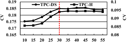
Figure 7. How CV (Coefficient of Variation) changes along with the increasing number of experimental samples for QCSA. The left and right Y axes represent the CVs of $TPC-DS$ and $TPC-H$, respectively.

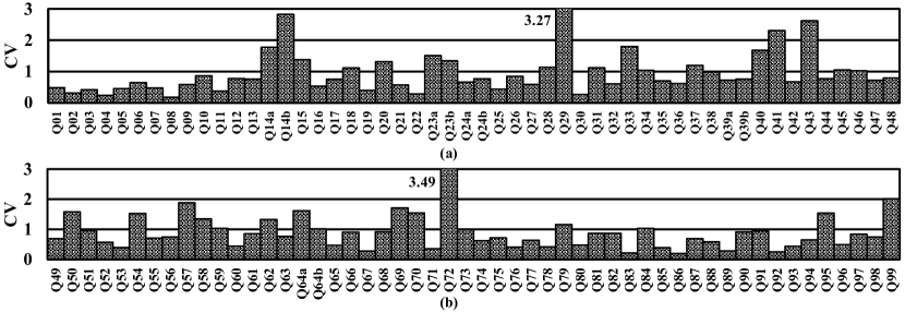
Figure 8. Configuration Sensitivity denoted by CV (coefficient variation) of the $TPC-DS$ queries. Y axis denotes the CVs of queries when configurations are changed.

5.1. Determining $N_{QCSA}$

As mentioned in Section 3.2, we need $N_{QCSA}$ of experimental samples to perform the query configuration sensitivity analysis (QCSA). To make the time used to collect experimental samples as short as possible, $N_{QCSA}$ should be as small as possible while it should also be large enough to accurately reflect the CV of the Spark SQL queries. We employ experiments to determine a suitable value of $N_{QCSA}$ to satisfy the above requirements. Figure 7 shows that how the CVs for $TPC-DS$ and $TPC-H$ change when we increase the number of experimental samples. As can be seen, when $N_{QCSA}$ increases from 10 to 30, the CV for $TPC-DS$ as well as that for $TPC-H$ keep increasing. When $N_{QCSA}$ is larger than 30, the CVs for both $TPC-DS$ and $TPC-H$ do not increase any longer. This indicates that 30 samples are enough for QCSA and more samples do not provide any information for CV besides wasting time. We therefore set $N_{QCSA}$ to 30 in this study. Note that we do not collect additional 30 experimental samples before we perform BO with DAGP (Dataisize-Aware Gaussian Process). Instead, we leverage the samples (executions) performed by the BO iterations.

5.2. QCSA Results and Analysis

After we set $N_{QCSA}$ to 30, we perform QCSA for $TPC-DS$ based on the 30 experimental samples. Figure 8 shows the CVs for the $104$ queries of $TPC-DS$. A couple of interesting findings can be observed here. For one, the CVs for different queries are significantly different. For example, the CV of query Q04 is only 0.24 while that of query Q72 is 3.49. We call the queries with small CVs configuration insensitive queries (CIQ) while others configuration sensitive queries (CSQ). This indicates that the performance of CIQs such as Q04 does not change much when the configuration changes while that of CSQs such as Q72 does. Second, long queries are not necessarily sensitive to configuration tuning. For example, the CV of query Q04 is relatively small (0.24) and its execution time is relatively long (e.g.,80 seconds) while the CV of query Q14b is relatively large (2.8) and its execution time is also relatively long (e.g.,49 seconds). This implies that removing long CIQs such as Q04 can significantly reduce the sample collection time when we collect experimental samples. This also indicates that tuning the configuration of long CSQs such as Q14b can improve performance more than tuning short queries with similar CVs. Why are some queries sensitive to configuration tuning while others are not? The reason is analyzed in Section 5.11.

Based on these findings, we remove queries by using the CV-based criteria introduced in Section 3.2 for experimental sample collection. For the $104$ queries in $TPC-DS$, we remove 81 queries and remain 23 queries when we collect experimental samples. The remaining 23 queries are {Q72, Q29, Q14b, Q43, Q41, Q99, Q57, Q33, Q14a, Q69, Q40, Q64a, Q50, Q21, Q70, Q95, Q54, Q23a, Q23b, Q15, Q58, Q62, Q20}. That is, we only execute 23 queries in each BO iteration with a different configuration during we search the optimal configuration for $TPC-DS$. As such, the time used to collect the experimental samples can be significantly reduced.

5.3. Determining $N_{IICP}$

To perform IICP, we need $N_{IICP}$ of experimental samples to observe how the performance of a Spark SQL application changes according to the value changes of each configuration parameter. Like $N_{QCSA}$, the value of $N_{IICP}$ should be as small as possible because our goal is to make the time for collection experimental samples short. On the other hand, $N_{IICP}$ should also be large enough to correctly identify the important parameters with respect to performance.

Again, we employ experiments to determine a suitable value for $N_{IICP}$. At the first step, we set $N_{IICP}$ to 5 and we therefore run a Spark SQL application five times, each time with a random configuration. The execution times of the five executions and their corresponding configurations are stored in matrix $S^{\prime}$ defined by equation (5). We then leverage CPS and CPE described in Section 3.3.2 to identify the important configuration parameters with respect to performance. We repeat this step a number of times with each time increasing $N_{IICP}$ by 5. We subsequently observe the number of the identified important configuration parameters. If the number of the parameters keeps constant and parameters remain the same when we perform the IICP with increasing values of $N_{IICP}$, it indicates that larger $N_{IICP}$ does not help correctly identify important configuration parameters. In our experiments, we tried ten values of $N_{IICP}$ (5, 10, 15, 20, 25, 30, 35, 40, 45, and 50). Figure 9 shows that the number of the identified important configuration parameters for $TPC-DS$ keeps the same when the value of $N_{IICP}$ is equal to or larger than 20. In addition, the important parameters are also the same when $N_{IICP}$ is larger than 20. We also perform the same experiment for $TPC-H$, Join, Scan, and Aggregation. We find the same phenomenon as shown in Figure 9 and we therefore set $N_{IICP}$ to 20 which is less than the value 30 that we set for $N_{QCSA}$. Note that we also take the executions in BO iterations as the experimental samples to perform IICP. Therefore, 30 experimental samples generated by BO iterations are enough for performing the QCSA and IICP of LOCAT.

Figure 10 shows the number of important configuration parameters identified by CPS and the ones further extracted by CPE. As can be seen, CPS selects about 2/3 of the original 38 configuration parameters as the important configuration parameters for five Spark SQL applications. CPE further extracts about 1/3 of the important configuration parameters selected by CPS. As a result, the number of configuration parameters fed to GP is significantly reduced and in turn the time used to search for the optimal configuration is accordingly dramatically decreased.

Figure 9. The number variation of identified important parameters along with the increasing number of samples.

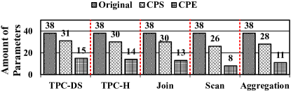
Figure 10. The number of important configuration parameters selected by CPS and CPE.

Table 3. Top 5 important configurations selected by $CPS$ with $100GB$, $500GB$, and $1TB$ input data size of $TPC-DS$.

Datasize	100GB	500GB	1TB
	sql.shuffle.partitions	sql.shuffle.partitions	sql.shuffle.partitions
Conf	executor.memory	shuffle.compress	shuffle.compress
(spark.)	executor.cores	executor.memory	executor.memory
	shuffle.compress	executor.instances	executor.instances
	executor.instances	executor.cores	memory.offHeap.size

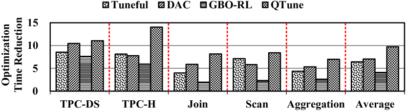
Figure 11. Optimization time comparison between LOCAT and others on the four-node ARM cluster. Y axis denotes the time reduction which is defined by using the optimization time taken by LOCAT to divide those taken by others.

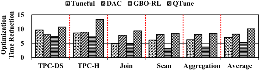
Figure 12. Optimization Time Comparison between LOCAT and others on the eight-node x86 cluster. Y axis denotes the time reduction which is defined by using the optimization time taken by LOCAT to divide those taken by others.

5.4. Important Parameter Examples

By using the technique CPS described in Section 3.3, we identify 15 important configuration parameters for the experimented benchmarks. Due to the space limitation, we show the five most important parameters for $TPC-DS$ with three input data sizes in Table 3. A couple of interesting findings can be made here. For one, the most important parameters for the three significantly different input data sizes are all spark.sql.shuffle.partitions. This parameter specifies the default number of partitions to use when shuffling data for joins or aggregations. Theoretically, this parameter’s value significantly influences the parallelism of shuffle operations, which in turn dramatically impacts the performance of a Spark SQL application.

Second, the three parameters related to the number of executor instances, memory size, and whether compress should be applied on shuffle operations are always in the top five important ones for the three input data sizes, their orders might be different though. The number of executor instances influences the task parallelism; the memory size controls the amount of memory can be used by Spark SQL tasks; and the compress influences the amount of data moved between the servers in the cluster, as well as between the memory and disks. Naturally, these aspects influence the performance of a Spark SQL application significantly.

Last but not the least, the parameter Spark.memory.offHeap.size comes to the fifth most important parameter when the data size increases to $1TB$. This is reasonable because the amount of memory can be used for off-heap allocation becomes important for performance when the input data size is large enough (e.g., $1TB$). In summary, these findings indicate that the important parameters with respect to performance found by IICP are convincible because we can find reasonable explanations for them.

5.5. Optimization Time

Figure 11 shows the optimization time reduction achieved by LOCAT on the ARM cluster, which is defined by using the optimization time taken by LOCAT to divide those taken by Tuneful, DAC, GBO-RL, and QTune. Note that the input data sizes for the benchmarks are all 300GB. As can be seen, the time taken by LOCAT to achieve the optimal performance of all benchmarks is significantly shorter than those used by other approaches. In detail, the times taken by Tuneful, DAC, GBO-RL, and QTune are $6.4\times$, $7.0\times$, $4.1\times$, and $9.7\times$ of the time used by LOCAT on average, and up to $7.9\times$, $8.9\times$, $6.3\times$, and $11.8\times$, respectively. Figure 12 shows the results on the x86 cluster. As can be seen, LOCAT reduces the optimization time taken by Tuneful, DAC, GBO-RL, and QTune by factors of $6.4\times$, $6.3\times$, $4.0\times$, and $9.2\times$ on average and up to $9.7\times$, $8.0\times$, $7.0\times$, and $10.3\times$, respectively. These results indicate two insights. First, LOCAT can indeed significantly reduce the time used by ML approaches to optimize the performance of a wide range of Spark SQL applications. Second, LOCAT can adapt to significantly different hardware as well as different scale of clusters.

The optimization time reduction made by LOCAT comes from LOCAT’s three innovations. 1) It leverages QCSA to eliminate the executions of configuration-insensitive queries in BO iterations, which significantly reduces the time for executing a Spark SQL application in each BO iteration. As a result, LOCAT significantly reduces the time used for collecting experimental samples. 2) LOCAT accelerates the BO convergence by developing IICP to reduce the dimension of the configuration searching space. 3) LOCAT leverages DAGP to adapt to the data size changes in optimization process, which enables LOCAT to reuse prior results with different input data sizes and in turn reduce the time overhead.

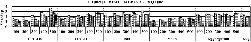
Figure 13. Speedups of the performance tuned by LOCAT over those tuned by Tuneful, DAC, GBO-RL, and QTune on the four-node ARM cluster. The unit of the numbers along with the X axis is GB. The Y axis represents the speedup which is defined by using the execution time of a program-input pair tuned by LOCAT to divide that of it tuned by another approach.

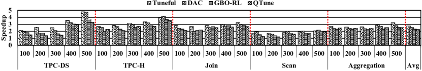
Figure 14. Speedups of the performance tuned by LOCAT over those tuned by other approaches on the eight-node x86 cluster. The unit of the numbers along with the X axis is GB. The Y axis represents the speedup which is defined by using the execution time of a program-input pair tuned by LOCAT to divide that of it tuned by another approach.

5.6. Speedup

Although LOCAT significantly reduces the optimization time needed by the state-of-the-art (SOTA) approaches, it is still unclear if it can achieve the performance tuned by the SOTA approaches. In this section, we compare the speedups of the program-input pairs tuned by LOCAT over they tuned by Tuneful, DAC, GBO-RL, and QTune. The speedup is defined as

(11) $$speedup=\frac{ET_{sota}}{ET_{locat}}$$

with $ET_{locat}$ and $ET_{sota}$ the execution times of a program-input pair tuned by LOCAT and by a SOTA approach, respectively.

Figure 13 shows the results on the four-node ARM cluster. As can be seen, LOCAT significantly improves the performance of the experimented 25 program-input pairs tuned by other SOTA approaches. In detail, the speedups of the program-input pairs tuned by LOCAT over they tuned by Tuneful, DAC, GBO-RL, and QTune are $2.4\times$, $2.2\times$, $2.0\times$, and $1.9\times$ on average, and up to $3.7\times$, $3.1\times$, $2.8\times$, and $2.4\times$, respectively. Figure 14 shows the results on the eight-node x86 cluster where LOCAT still significantly outperforms the SOTA approaches in terms of performance. In detail, LOCAT improves the 25 program-input pairs’ performance tuned by Tuneful, DAC, GBO-RL, and QTune by factors of $2.8\times$, $2.6\times$, $2.3\times$, and $2.1\times$ on average, and up to $4.8\times$, $4.7\times$, $3.7\times$, and $3.3\times$, respectively.

A couple of conclusions can be made from these speedups in addition to the optimization time reductions. For one, LOCAT can tune Spark SQL applications with not only higher performance improvements but also in significantly shorter time compared to the SOTA approaches. Second, on significantly different hardware and different scales of clusters, LOCAT can still outperform the SOTA approaches in both performance improvement and optimization time reduction. Third, LOCAT outperforms the SOTA approaches for all different input data sizes of a Spark SQL application, as shown in Figure 13 and Figure 14. Last, LOCAT generally improves the performance more for the larger input data size of a Spark SQL application compared to the SOTA approaches. These benefits make LOCAT more suitable for optimizing future Spark SQL applications because the input data size of them is getting increasingly larger.

Figure 15. The performance of TPC-DS with input data sizes of 100GB, 200GB, 300GB, 400GB, and 500GB tuned by LOCAT with all parameters (AP) and important parameters (IP).

Although LOCAT’s primary goal is to reduce the optimization time of ML-based tuning approaches for Spark SQL applications, it surprisingly shows performance improvements. This is because LOCAT identifies the important configuration parameters to tune performance. Tuning more configuration parameters does not necessarily result in higher performance. Instead, it may degrade performance because the unimportant parameters may counteract the performance improvements caused by tuning the important ones. We conduct experiments to confirm this. We compare the performance of TPC-DS with input data sizes of 100GB, 200GB, 300GB, 400GB, and 500GB tuned by LOCAT with all the 38 configuration parameters (AP) and with the 15 important parameters (IP) produced by IICP. Figure 15 shows the results. As can be seen, The performance achieved by tuning the 15 important parameters is $1.8\times$ higher than that turned by all the 38 parameters on average. This confirms that tuning the important configuration parameters results in higher performance than tuning all the configuration parameters for Spark SQL applications.

5.7. Why IICP?

IICP is designed to identify the important configuration parameters with respect to performance. In fact, a lot of machine learning (ML) algorithms can also be used for this purpose. For example, Gradient Boosting Regression Tree (GBRT) has been used to quantify the importance of CPU performance events (Lv et al., 2018). Why do we design IICP for the same purpose? To answer this question, we evaluate if our IICP approach is better than ML-based approaches.

To identify important configuration parameters, ML-based approaches need to build an accurate performance model as a function of the parameters first. Subsequently, the importance of a parameter is calculated by using the performance model. Higher accuracy of a performance model generally indicates the parameter importance calculated from it is more convincible. We therefore use several ML algorithms to construct performance models and use the mean squared error (MSE) (Marmolin, 1986) to measure the model accuracy.

Figure 16 shows the accuracy of the performance models built by Gradient Boosting Regression Tree (GBRT), Support Vector Regression (SVR), Linear Regression (LinearR), Logistic Regression (LR), and K-Nearest Neighbor Algorithm for Regression (KNNAR). Note that these models are trained by using the same training data set. As can be seen, the average error of the GBRT models is less than 15%, which is the lowest among all models built by other ML algorithms for all workloads. This indicates that the configuration parameter importance calculated by GBRT models is more convincible than by other ML algorithms. We therefore compare IICP against the models built by GBRT.

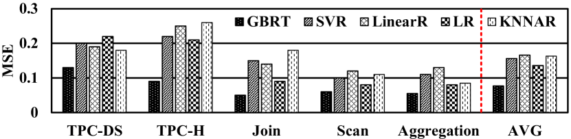
Figure 16. Accuracy of models built by GBRT (Gradient Boosted Regression Tree), SVR (Support Vector Regression), LinearR (Linear Regression), LR (Logistic Regression), and KNNAR (K-Nearest Neighbor Algorithm for Regression).

After we identify the important configuration parameters by our IICP and the GBRT model, we use them to configure $TPC-DS$ with 100GB of input data and execute the program a number of times, each time with a different random configuration. Note that the configurations only contain the values of the identified important parameters. We run $TPC-DS$ for $5$, $10$, $15$, $20$, $25$, and $30$ times and observe the standard deviations of its execution times.

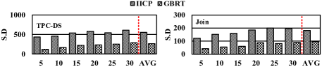
Figure 17. The comparison between IICP and GBRT. The Y axis represents the standard deviation of the execution times of $TPC-DS$ and $Join$ configured by the important parameters identified by IICP or GBRT.

The results are shown in Figure 17, where the $Y$ axis represents the SD (standard deviation) of execution times of $TPC-DS$ and Join configured by the important parameters identified by IICP and GBRT, and the $X$ axis represents the number of executions. Higher SD of execution times indicates that configuration parameters identified by the approach are more important than one another. We find that, the SD of IICP is significantly higher than that of GBRT. This indicates that IICP outperforms GBRT for identifying important parameters, especially with low overhead. The reason is that GBRT requires a large number of experiment samples to build an accurate model while IICP does not, and IICP employs a novel hybrid approach combining the feature selection and feature extraction.

5.8. Where does the Speedup Come from?

We now analyze where the speedup made by LOCAT come from. Figure 18 shows the execution time of CSQ (Configuration Sensitive Query) and CIQ (Configuration Insensitive Query) of $TPC-DS$ including $104$ queries. A number of interesting observations can be made here. First, LOCAT, Tuneful, DAC, GBO-RL, and QTune all reduce the execution time significantly and the performance is higher with larger input data size. Second, the performance improvement mainly comes from reducing the execution time of CSQ. This is because CIQ is hard to optimize by tuning the configuration parameters. Third, LOCAT outperforms other four methods in reducing more executing time of CSQ. This is because: 1) LOCAT leverages IICP to identify the important parameters and focuses on tuning them, which achieves higher performance improvements as shown in Section 5.6; 2) LOCAT distinguishes CIQ between CSQ and avoids executing CIQ to concentrate more on CSQ tuning while other methods is not able to do so; 3) LOCAT takes the size of input data as a prior knowledge of BO to determine current optimal parameter online during the iteration of BO.

Furthermore, we find that the speedup made by LOCAT over other SOTA approaches mainly comes from that LOCAT reduces the garbage collection (GC) time significantly more than other approaches. Figure 19 (a) and (b) show the GC time comparison for $TPC-DS$ with multiple queries and Join with one query, respectively. As can be seen, the JVM GC time used by LOCAT is significantly shorter than other approaches no matter in with multiple queries or with only one query. In addition, the GC time used by LOCAT increases significantly slowly than other approaches with the increasing of input data size. This is because GC dynamically performs several memory operations such as allocating from or releasing memory to the operating system according to an application’s request. LOCAT sets more proper values for the memory related parameters, making GC spend less time to perform the memory operations than other approaches. This also indicates that LOCAT would have more benefits if larger data set is processed.

5.9. Tuning Overhead of Increasing Data Size

Figure 20 compares the optimization overhead when LOCAT and the SOTA approaches are applied to TPC-DS with increasing input data size. As can be seen, LOCAT incurs significantly lower optimization overhead for all different sizes of input data. The optimization time reduction compared to other SOTA applications made by LOCAT becomes more when the data size increases. The reason is that LOCAT adapts to the input data size changes to avoid re-tuning, which is similar to but better than Tuneful that directly uses BO without adapting data size changes, and GBO-RL that leverages a more time-consuming reinforcement learning (RL).

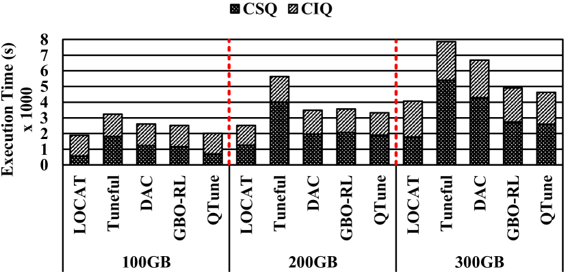
Figure 18. LOCAT Outperforms other Approaches by Significantly Accelerating the Execution of CSQ.

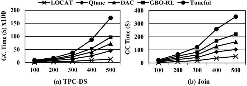
Figure 19. JVM Garbage Collection (GC) Time Comparison.

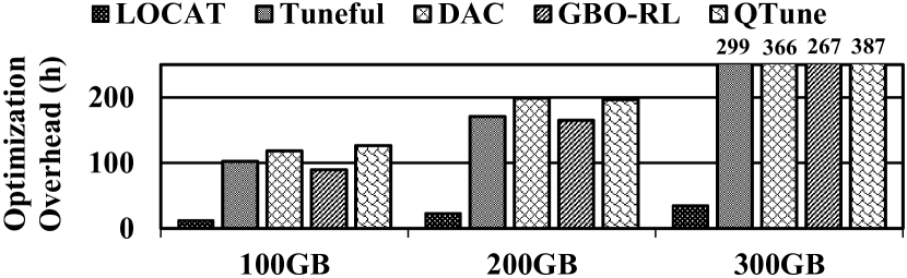
Figure 20. How Tuning Overhead (in hours) Changes when the input data size of an application increases.

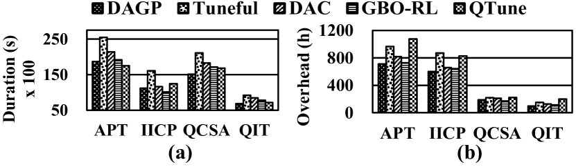
Figure 21. Optimized Performance and Optimization Overhead Comparison between DAGP, Tuneful, DAC, GBO-RL, and Qtune. APT represents all parameters tuning. QIT denotes tuning performance with QCSA and IICP.

5.10. Using IICP/QCSA on SOTA Approaches

Although QCSA and IICP are designed to work with DAGP, they can definitely be applied on other SOTA approaches. We therefore combine Tuneful, DAC, GBO-RL, and QTune with all parameter tuning (APT), QCSA, and IICP to form new approaches first. We subsequently apply these approaches on $TPC-DS$ with 500GB of input data to compare the optimized performance and the optimization overhead. Figure 21 shows the result. As can be seen, IICP reduces the execution times of the five approaches by factors of $1.7\times$ on average and up to $1.9\times$ (Figure 21 (a)), and decreases the optimization overhead by factors of $1.2\times$ on average and up to $1.3\times$ (Figure 21 (b)). QCSA improves the performance of TPC-DS tuned by the five approaches by factors of $1.3\times$ on average and up to $1.4\times$ and reduces their optimization overhead by factors of $4.2\times$ and up to $4.8\times$. Moreover, we find that IICP with QCSA can further improve the performance by a factor of $2.6\times$ on average and up to $2.9\times$, and decreases the optimization overhead by a factor of $6.8\times$ on average and up to $9.1\times$. These results indicate that our IICP and QCSA techniques can be used in other ML approaches to tune the performance with low overhead.

5.11. Reasons for Config In/Sensitive Queries

We now analyze why some queries are configuration sensitive while others are not. According to (Pavlo et al., 2009), queries can be divided into three categories: ‘selection’, ‘join’, and ‘aggregation’. Most simple ‘selection’ queries are configuration insensitive because they do not consume a large amount of computing and memory resources specified by the configuration parameters. For example, in TPC-DS with 100GB of input data, {Q09, Q13, Q16, Q28, Q32, Q38, Q48, Q61, Q84, Q87, Q88, Q94, and Q96} are ’selection’ queries which perform a simple filter logic and only consume 5 CPU cores and 8GB memory on average to achieve their optimal performance. Tuning the resource related configuration parameters for them therefore does not influence their performance significantly. Moreover, these queries do not process or move a large amount of data. The configuration parameter related to “compress” data therefore does not affect the performance significantly.

However, the queries belonging to categories ‘join’ and ‘aggregation’ involve shuffle operations which generally consume compute, memory, and network resources specified by configuration parameters. If the shuffle operations of a query process a large amount of data, the query is configuration sensitive. Otherwise, the query is configuration insensitive. For example, in $TPC-DS$ with 100GB of input data, the shuffle operations of $Q72$ process 52GB of data. $Q72$ is therefore configuration sensitive. In contrast, the shuffle operations of $Q08$ process only 5MB of data, $Q08$ is therefore insensitive.

5.12. Parameter Value Range Determination

When we tune configuration parameters for optimal performance of a Spark SQL application, it is important to know the value range of each parameter. However, this is difficult because the value ranges of some parameters depend on the cluster resources while others depend on the program logic. To address these difficulties, we firstly classify the 38 configuration parameters into 28 numeric parameters (in bold text in Table 2) and 10 non-numeric ones (others in Table 2). Since the values of non-numeric parameters are always True or False, we do not determine the value ranges for them and instead focus on the numeric parameters.

Subsequently, we further classify the numerical parameters into resource (e.g., CPU core # and memory size) parameters (with $*$ in Table 2), and non-resource parameters (in bold text without $*$ in Table 2). Next, we determine the value range of a resource parameter according to the memory size and core # in total in the cluster and the maximum resource capacity of the container specified by cluster managers such as Yarn (Vavilapalli et al., 2013), Kubernetes (Bernstein, 2014), and Mesos (Hindman et al., 2011). For example, in Yarn mode, the value range of spark.executor.cores and spark.driver.cores is the same as that of CPU core capacity of Yarn container. As for memory related parameters, the value range of spark.driver.memory and spark.executor.memory is the same as that of memory capacity of Yarn container. The value range of spark.executor.memoryOverhead and spark.memory.offHeap.size is from 0 to the maximum of memory capacity of Yarn container, which is determined by time-consuming experiments. Moreover, we control the sum of parameters spark.executor.memory, spark.executor.
memoryOverhead, and spark.memory.offHeap.size, the total memory resource of a single process, to be smaller than the memory capacity of the Yarn container. In addition, we also specify the product of spark.executor.instances and the resource amount of a single process to be less than the total amount of resources in the cluster. As such, the value ranges of the resource parameters can be determined.

As for the non-resource parameters, we determine their value range based on a time-consuming experiment. Starting from the default value ($dv$) of a parameter, we try values larger or smaller than the $dv$ with $N$ times. The value of $N^{th}$ time is $dv+N*step$ when we try to determine the upper bound. Likewise, the value is $dv-N*step$ when we try to determine the lower bound. $step$ is the stride value. If a program can not start to run or hung when we configure the value of a parameter as $dv+N*step$ or $dv-N*step$, we set the upper bound or lower bound of the parameter as $dv+(N-1)*step$ or $dv-(N-1)*step$, respectively.

6. Related Work

In this section, we describe the configuration auto-tuning studies related to Spark SQL. A large body of automatic parameter tuning approaches can be applied to Spark SQL, which are divided into six categories (Herodotou et al., 2020): 1) Rule-based approaches (RBA) tune performance based on the expert experience, online tutorials (SparkConf, 2022), or tuning guidebooks (SparkTuning, 2022) which are time-consuming and labour-intensive because using RBA requires a deep understanding of system internals, while LOCAT does not. 2) Cost modeling approaches’ (CMA) (Wang and Khan, 2015; Venkataraman et al., 2016; Zacheilas et al., 2017; Singhal and Singh, 2018; Gounaris et al., 2017; Chen et al., 2019b) build performance prediction models with analytical model which are not able to be applied to the complex system like Spark SQL and adapt to the input data size changing, while LOCAT is able to. 3) Simulation-based approaches (SBA) (Ardagna et al., 2021; De Almeida et al., 2019; de Almeida et al., 2018; Karimian-Aliabadi et al., 2019) build performance prediction models based on simulation of optimized system which are not suitable for complex system like Spark SQL. 4) Experiment-driven approaches (EDA) (Petridis et al., 2017; Zhu et al., 2017; Gounaris et al., 2017; Bao et al., 2018; Yu et al., 2018) find the optimal configuration by executing an application repeatedly with different configuration parameters until converge, which causes high overhead, while LOCAT really takes optimization overhead into consideration and significantly reduces it. 5) Machine learning approaches (MLA) (Wang et al., 2016; Álvaro Brandón Hernández et al., 2018; Jia et al., 2016; Chen et al., 2019a) build performance prediction models by machine learning algorithms, needing to collect a large number of training samples with high overhead, while LOCAT achieves high optimization performance with significantly low overhead. 6) Adaptive approaches (AA) (Fekry et al., 2020; Suraweera and Mitrovic, 2002; Li et al., 2018; Kunjir and Babu, 2020) tune the configuration parameter with adaptivity to dynamic runtime status (e.g., input data size changing). AA does not consider the optimization overhead while LOCAT does.

From above, we can find that current approaches still face two problems: First, high overhead of the optimization process. Second, unadaptability of optimal configuration to different input data sizes. We now summarize studies trying to solve the two problems.

6.1. Reducing Optimization Overhead

Leveraging ML-based performance models to avoid actually executing an application is an effective way to reduce the cost of searching for the optimal configuration for the application. RFHOC (Bei et al., 2016) and DAC (Yu et al., 2018) are the examples of such approaches. However, it is time-consuming to build a performance model because we need to collect a large number of training samples by executing the application on a real cluster with a random configuration each time. LOCAT differs from these approaches by innovating QCSA and IICP to reduce the time used for collecting training samples.

Another line of studies to accelerate the optimization process are to combine an analytical model or the application characteristics with a ML algorithm. For example, GBO-RL (Kunjir and Babu, 2020) builds an analytical model for Spark’s memory management to speed up the BO convergence. But GBO-RL only considers memory and the analytical model is inaccurate (Yu et al., 2018). In contrast, LOCAT considers all layers of configuration parameters of Spark SQL applications. Another work, Tuneful (Fekry et al., 2020), uses One-at-a-time (OAT) method to identify a subspace composed of configurations that significantly influence Spark performance as the searching space, which directly reduces the dimension of the search space to speed the optimization process up. But Tuneful is not suitable for high-dimensional configuration scenarios because the number of iterations of OAT increases rapidly when the number of configuration parameters increases.

6.2. Adapting to Input Data Size Changes

Some performance tuning studies for big data systems try to adapt to input data size changes indirectly or directly. For instance, KERMIT (Suraweera and Mitrovic, 2002) works at YARN level to dynamically adapt to the resource allocation, including memory and CPU cores of containers. It randomly searches an optimal resource configuration by observing the container’s performance changing in real-time. But KERMIT is limited to optimize memory configuration only and the random searching is always time-consuming. (Prats et al., 2020) is able to optimize the unseen workload without retraining by leveraging a performance model enhanced by using the execution log. It generalizes to different workloads (with different logical or input data) by extracting information in stages and tasks to provide a general model for all kinds of applications in Spark. But (Prats et al., 2020) becomes impractical when there is a shortage of log files. QTune (Li et al., 2018) realizes adaptive optimization by leveraging deep reinforcement learning (Sutton and Barto, 1998), and QTune needs to characterize each query of an application for high performance. CDBTune (Zhang et al., 2019) is similar to QTune, leveraging deep reinforcement learning. They both are too time-consuming to be applied in practice.

Differing from these studies, LOCAT realizes adaptive optimization for Spark SQL applications by developing a Data size Aware Gaussian Process (DAGP) which considers the input data size in Gaussian Process. Moreover, LOCAT significantly reduces the optimization overhead and outperforms these approaches in high-dimensional configuration spaces.

7. Conclusion

This paper proposes LOCAT, a BO-based approach that efficiently as well as adaptively finds the optimal configurations to achieve high performance for a Spark SQL application on a given cluster. LOCAT innovates three techniques: query configuration sensitive analysis (QCSA), identifying important configuration parameters (IICP), and data size aware Gaussian Process (DAGP). The experiments on two significantly different clusters, a four-node ARM cluster and an eight-node x86 cluster, show that LOCAT can significantly reduce the optimization time of the state-of-the-art approaches and dramatically improve performance over them.

8. Acknowledgements

This work is supported by the Key-Area Research and Development Program of Guangdong Province (Grant No. 2019B010155003), and is partially supported by the Shenzhen Institute of Artificial Intelligence and Robotics for Society (AIRS), Chinese University of Hong Kong, Shenzhen.

References

- (1)
- Akoglu (2018) Haldun Akoglu. 2018. User’s guide to correlation coefficients. Turkish Journal of Emergency Medicine 18, 3 (2018), 91–93. https://doi.org/10.1016/j.tjem.2018.08.001
- Alipourfard et al. (2017) Omid Alipourfard, Hongqiang Harry Liu, Jianshu Chen, Shivaram Venkataraman, Minlan Yu, and Ming Zhang. 2017. Cherrypick: Adaptively Unearthing the Best Cloud Configurations for Big Data Analytics. In Proceedings of the 14th USENIX Conference on Networked Systems Design and Implementation (Boston, MA, USA) (NSDI’17). USENIX Association, USA, 469–482. https://www.usenix.org/conference/nsdi17/technical-sessions/presentation/alipourfard
- Ardagna et al. (2021) D. Ardagna, E. Barbierato, E. Gianniti, M. Gribaudo, T. B.M. Pinto, A. P.C. da Silva, and J. M. Almeida. 2021. Predicting the performance of big data applications on the cloud. Journal of Supercomputing 77, 2 (2021), 1321–1353. https://doi.org/10.1007/s11227-020-03307-w
- Armbrust et al. (2015) Michael Armbrust, Reynold S. Xin, Cheng Lian, Yin Huai, Davies Liu, Joseph K. Bradley, Xiangrui Meng, Tomer Kaftan, Michael J. Franklin, Ali Ghodsi, and Matei Zaharia. 2015. Spark SQL: Relational Data Processing in Spark. In Proceedings of the 2015 ACM SIGMOD International Conference on Management of Data (Melbourne, Victoria, Australia) (SIGMOD ’15). Association for Computing Machinery, New York, NY, USA, 1383–1394. https://doi.org/10.1145/2723372.2742797
- Baldacci and Golfarelli (2019) Lorenzo Baldacci and Matteo Golfarelli. 2019. A Cost Model for SPARK SQL. IEEE Transactions on Knowledge and Data Engineering 31, 5 (2019), 819–832. https://doi.org/10.1109/TKDE.2018.2850339
- Bao et al. (2018) Liang Bao, Xin Liu, and Weizhao Chen. 2018. Learning-based Automatic Parameter Tuning for Big Data Analytics Frameworks. In 2018 IEEE International Conference on Big Data (Big Data). 181–190. https://doi.org/10.1109/BigData.2018.8622018
- Barata et al. (2015) Melyssa Barata, Jorge Bernardino, and Pedro Furtado. 2015. An overview of decision support benchmarks: TPC-DS, TPC-H and SSB. Advances in Intelligent Systems and Computing 353 (2015), 619–628. https://doi.org/10.1007/978-3-319-16486-1_61
- Bei et al. (2016) Zhendong Bei, Zhibin Yu, Huiling Zhang, Wen Xiong, Chengzhong Xu, Lieven Eeckhout, and Shengzhong Feng. 2016. RFHOC: A Random-Forest Approach to Auto-Tuning Hadoop’s Configuration. IEEE Transactions on Parallel and Distributed Systems 27, 5 (2016), 1470–1483. https://doi.org/10.1109/TPDS.2015.2449299
- Bernstein (2014) David Bernstein. 2014. Containers and Cloud: From LXC to Docker to Kubernetes. IEEE Cloud Computing 1, 3 (2014), 81–84. https://doi.org/10.1109/MCC.2014.51
- Bhattacharyya et al. (1979) Helen T. Bhattacharyya, David G. Kleinbaum, and Lawrence L. Kupper. 1979. Applied Regression Analysis and Other Multivariable Methods. Vol. 74. Cengage Learning. 732 pages. https://doi.org/10.2307/2287012
- Bolboaca and Jäntschi (2006) Sorana-Daniela Bolboaca and Lorentz Jäntschi. 2006. Pearson versus Spearman, Kendall’s tau correlation analysis on structure-activity relationships of biologic active compounds. Leonardo Journal of Sciences 5, 9 (2006), 179–200. http://ljs.academicdirect.org/A09/179_200.htm
- Boncz et al. (2014) Peter Boncz, Thomas Neumann, and Orri Erling. 2014. TPC-H analyzed: Hidden messages and lessons learned from an influential benchmark. In Lecture Notes in Computer Science (including subseries Lecture Notes in Artificial Intelligence and Lecture Notes in Bioinformatics), Vol. 8391 LNCS. Springer, 61–76. https://doi.org/10.1007/978-3-319-04936-6_5
- Chandrashekar and Sahin (2014) Girish Chandrashekar and Ferat Sahin. 2014. A survey on feature selection methods. Computers & Electrical Engineering 40, 1 (2014), 16–28. https://doi.org/10.1016/j.compeleceng.2013.11.024 40th-year commemorative issue.
- Chen et al. (2019a) Yuxing Chen, Peter Goetsch, Mohammad A. Hoque, Jiaheng Lu, and Sasu Tarkoma. 2019a. d-Simplexed: Adaptive Delaunay Triangulation for Performance Modeling and Prediction on Big Data Analytics. IEEE Transactions on Big Data (2019), 1–1. https://doi.org/10.1109/tbdata.2019.2948338
- Chen et al. (2019b) Yuxing Chen, Jiaheng Lu, Chen Chen, Mohammad Hoque, and Sasu Tarkoma. 2019b. Cost-effective resource provisioning for spark workloads. In International Conference on Information and Knowledge Management, Proceedings. 2477–2480. https://doi.org/10.1145/3357384.3358090
- Cheng et al. (2021) Keyang Cheng, Muhammad Saddam Khokhar, Misbah Ayoub, and Zakria Jamali. 2021. Nonlinear dimensionality reduction in robot vision for industrial monitoring process via deep three dimensional Spearman correlation analysis (D3D-SCA). Multimedia Tools and Applications 80, 4 (2021), 5997–6017. https://doi.org/10.1007/s11042-020-09859-6
- Chiba and Onodera (2016) Tatsuhiro Chiba and Tamiya Onodera. 2016. Workload characterization and optimization of TPC-H queries on Apache Spark. In ISPASS 2016 - International Symposium on Performance Analysis of Systems and Software. IEEE, 112–121. https://doi.org/10.1109/ISPASS.2016.7482079
- Chiba et al. (2018) Tatsuhiro Chiba, Takeshi Yoshimura, Michihiro Horie, and Hiroshi Horii. 2018. Towards Selecting Best Combination of SQL-on-Hadoop Systems and JVMs. In IEEE International Conference on Cloud Computing, CLOUD, Vol. 2018-July. IEEE, 245–252. https://doi.org/10.1109/CLOUD.2018.00038
- Cuzzocrea (2015) Alfredo Cuzzocrea. 2015. Data warehousing and OLAP over Big Data: a survey of the state-of-the-art, open problems and future challenges. International Journal of Business Process Integration and Management 7, 4 (2015), 372–377. https://doi.org/10.1504/IJBPIM.2015.073665 arXiv:https://www.inderscienceonline.com/doi/pdf/10.1504/IJBPIM.2015.073665
- de Almeida et al. (2018) Leandro Batista de Almeida, Eduardo Cunha de Almeida, John Murphy, Robson E. De Grande, and Anthony Ventresque. 2018. BigDataNetSim: A Simulator for Data and Process Placement in Large Big Data Platforms. In 2018 IEEE/ACM 22nd International Symposium on Distributed Simulation and Real Time Applications (DS-RT). 1–10. https://doi.org/10.1109/DISTRA.2018.8601018
- De Almeida et al. (2019) Leandro Batista De Almeida, Damien Magoni, Philip Perry, Eduardo Cunha De Almeida, John Murphy, and Anthony Ventresque. 2019. Multi-Layer-Mesh: A Novel Topology and SDN-Based Path Switching for Big Data Cluster Networks. In IEEE International Conference on Communications, Vol. 2019-May. IEEE, 1–7. https://doi.org/10.1109/ICC.2019.8761785
- Fekry et al. (2020) Ayat Fekry, Lucian Carata, Thomas Pasquier, Andrew Rice, and Andy Hopper. 2020. Tuneful: An Online Significance-Aware Configuration Tuner for Big Data Analytics. arXiv preprint arXiv:2001.08002 (2020). arXiv:2001.08002 http://arxiv.org/abs/2001.08002
- Gounaris et al. (2017) Anastasios Gounaris, Georgia Kougka, Ruben Tous, Carlos Tripiana Montes, and Jordi Torres. 2017. Dynamic configuration of partitioning in spark applications. IEEE Transactions on Parallel and Distributed Systems 28, 7 (2017), 1891–1904. https://doi.org/10.1109/TPDS.2017.2647939
- Guyon et al. (2008) Isabelle Guyon, Steve Gunn, Masoud Nikravesh, and Lofti A Zadeh. 2008. Feature extraction: foundations and applications. Vol. 207. Springer. https://eprints.soton.ac.uk/261922/
- Hao et al. (2013) Wangli Hao, Jianwu Li, and Xiao Zhang. 2013. Learning KPCA for face recognition. In Communications in Computer and Information Science, Vol. 375. Springer, 142–146. https://doi.org/10.1007/978-3-642-39678-6_24
- Helton and Davis (2003) J.C. Helton and F.J. Davis. 2003. Latin hypercube sampling and the propagation of uncertainty in analyses of complex systems. Reliability Engineering & System Safety 81, 1 (2003), 23–69. https://doi.org/10.1016/S0951-8320(03)00058-9
- Herodotou et al. (2020) Herodotos Herodotou, Yuxing Chen, and Jiaheng Lu. 2020. A Survey on Automatic Parameter Tuning for Big Data Processing Systems. ACM Comput. Surv. 53, 2, Article 43 (apr 2020), 37 pages. https://doi.org/10.1145/3381027
- Hindman et al. (2011) Benjamin Hindman, Andy Konwinski, Matei Zaharia, Ali Ghodsi, Anthony D. Joseph, Randy Katz, Scott Shenker, and Ion Stoica. 2011. Mesos: A Platform for Fine-Grained Resource Sharing in the Data Center. In Proceedings of the 8th USENIX Conference on Networked Systems Design and Implementation (Boston, MA) (NSDI’11). USENIX Association, USA, 295–308. https://dl.acm.org/doi/abs/10.5555/1972457.1972488
- Hoffman et al. (2011) Matthew Hoffman, Eric Brochu, Nando de Freitas, et al. 2011. Portfolio Allocation for Bayesian Optimization.. In UAI. Citeseer, 327–336. https://dl.acm.org/doi/abs/10.5555/3020548.3020587
- Hsu et al. (2018) Chin-Jung Hsu, Vivek Nair, Vincent W. Freeh, and Tim Menzies. 2018. Arrow: Low-Level Augmented Bayesian Optimization for Finding the Best Cloud VM. In 2018 IEEE 38th International Conference on Distributed Computing Systems (ICDCS). 660–670. https://doi.org/10.1109/ICDCS.2018.00070
- Huang et al. (2010) Shengsheng Huang, Jie Huang, Jinquan Dai, Tao Xie, and Bo Huang. 2010. The HiBench benchmark suite: Characterization of the MapReduce-based data analysis. In 2010 IEEE 26th International Conference on Data Engineering Workshops (ICDEW 2010). 41–51. https://doi.org/10.1109/ICDEW.2010.5452747
- Ivanov and Beer (2015) Todor Ivanov and Max-Georg Beer. 2015. Evaluating Hive and Spark SQL with BigBench. arXiv preprint arXiv:1512.08417 (2015). arXiv:1512.08417 http://arxiv.org/abs/1512.08417
- Jia et al. (2016) Zhen Jia, Chao Xue, Guancheng Chen, Jianfeng Zhan, Lixin Zhang, Yonghua Lin, and Peter Hofstee. 2016. Auto-tuning Spark big data workloads on POWER8: Prediction-based dynamic SMT threading. In 2016 International Conference on Parallel Architecture and Compilation Techniques (PACT). 387–400. https://doi.org/10.1145/2967938.2967957
- Jones et al. (1998) Donald R. Jones, Matthias Schonlau, and William J. Welch. 1998. Efficient Global Optimization of Expensive Black-Box Functions. Journal of Global Optimization 13, 4 (1998), 455–492. https://doi.org/10.1023/A:1008306431147
- Karimian-Aliabadi et al. (2019) Soroush Karimian-Aliabadi, Danilo Ardagna, Reza Entezari-Maleki, and Ali Movaghar. 2019. Scalable Performance Modeling and Evaluation of MapReduce Applications. In High-Performance Computing and Big Data Analysis, Lucio Grandinetti, Seyedeh Leili Mirtaheri, and Reza Shahbazian (Eds.). Springer International Publishing, Cham, 441–458. https://doi.org/10.1007/978-3-030-33495-6_34
- Kunjir and Babu (2020) Mayuresh Kunjir and Shivnath Babu. 2020. Black or White? How to Develop an AutoTuner for Memory-Based Analytics. In Proceedings of the 2020 ACM SIGMOD International Conference on Management of Data (Portland, OR, USA) (SIGMOD ’20). Association for Computing Machinery, New York, NY, USA, 1667–1683. https://doi.org/10.1145/3318464.3380591
- Li et al. (2018) Guoliang Li, Xuanhe Zhou, Shifu Li, and Bo Gao. 2018. QTune: A QueryAware database tuning system with deep reinforcement learning. Proceedings of the VLDB Endowment 12, 12 (2018), 2118–2130. https://doi.org/10.14778/3352063.3352129
- Lorenzo et al. (2015) Jose Carlos Lorenzo, Lourdes Yabor, Norma Medina, Nicolas Quintana, and Vanessa Wells. 2015. Coefficient of variation can identify the most important effects of experimental treatments. Notulae Botanicae Horti Agrobotanici Cluj-Napoca 43, 1 (2015), 287–291. https://www.notulaebotanicae.ro/index.php/nbha/article/view/9881/7790
- Lv et al. (2015) Yanfei Lv, Huihong He, Yasong Zheng, Zhe Liu, and Hong Zhang. 2015. OLAP query performance tuning in Spark. In Third International Conference on Cyberspace Technology (CCT 2015). 1–5. https://doi.org/10.1049/cp.2015.0832
- Lv et al. (2018) Yirong Lv, Bin Sun, Qingyi Luo, Jing Wang, Zhibin Yu, and Xuehai Qian. 2018. Counterminer: Mining big performance data from hardware counters. In 2018 51st Annual IEEE/ACM International Symposium on Microarchitecture (MICRO). IEEE, 613–626. https://doi.org/10.1109/MICRO.2018.00056
- Marmolin (1986) Hans Marmolin. 1986. Subjective Mse Measures. IEEE Transactions on Systems, Man and Cybernetics SMC-16, 3 (1986), 486–489. https://doi.org/10.1109/tsmc.1986.4308985
- Mika et al. (1998) Sebastian Mika, Bernhard Schölkopf, Alex Smola, Klaus-Robert Müller, Matthias Scholz, and Gunnar Rätsch. 1998. Kernel PCA and De-Noising in Feature Spaces. In Advances in Neural Information Processing Systems, M. Kearns, S. Solla, and D. Cohn (Eds.), Vol. 11. MIT Press. https://proceedings.neurips.cc/paper/1998/file/226d1f15ecd35f784d2a20c3ecf56d7f-Paper.pdf
- Mockus (2012) Jonas Mockus. 2012. Bayesian approach to global optimization: theory and applications. Vol. 37. Springer Science & Business Media. https://doi.org/10.1007/978-94-009-0909-0
- Pavlo et al. (2009) Andrew Pavlo, Erik Paulson, Alexander Rasin, Daniel J. Abadi, David J. DeWitt, Samuel Madden, and Michael Stonebraker. 2009. A Comparison of Approaches to Large-Scale Data Analysis. In Proceedings of the 2009 ACM SIGMOD International Conference on Management of Data (Providence, Rhode Island, USA) (SIGMOD ’09). Association for Computing Machinery, New York, NY, USA, 165–178. https://doi.org/10.1145/1559845.1559865
- Petridis et al. (2017) Panagiotis Petridis, Anastasios Gounaris, and Jordi Torres. 2017. Spark Parameter Tuning via Trial-and-Error. In Advances in Big Data, Plamen Angelov, Yannis Manolopoulos, Lazaros Iliadis, Asim Roy, and Marley Vellasco (Eds.). Springer International Publishing, Cham, 226–237. https://doi.org/10.1007/978-3-319-47898-2_24
- Prats et al. (2020) David Buchaca Prats, Felipe Albuquerque Portella, Carlos H.A. Costa, and Josep Lluis Berral. 2020. You only Run Once: Spark Auto-Tuning from a Single Run. IEEE Transactions on Network and Service Management 17, 4 (2020), 2039–2051. https://doi.org/10.1109/TNSM.2020.3034824
- Ramdane et al. (2019) Yassine Ramdane, Omar Boussaid, Nadia Kabachi, and Fadila Bentayeb. 2019. Partitioning and Bucketing Techniques to Speed up Query Processing in Spark-SQL. In Proceedings of the International Conference on Parallel and Distributed Systems - ICPADS, Vol. 2018-Decem. IEEE, 142–151. https://doi.org/10.1109/PADSW.2018.8644891
- Rasmussen (2004) Carl Edward Rasmussen. 2004. Gaussian Processes in machine learning. In Lecture Notes in Computer Science (including subseries Lecture Notes in Artificial Intelligence and Lecture Notes in Bioinformatics), Vol. 3176. Springer, 63–71. https://doi.org/10.1007/978-3-540-28650-9_4
- Rida (2020) Qayyum Rida. 2020. A Roadmap Towards Big Data Opportunities, Emerging Issues and Hadoop as a Solution. International Journal of Education and Management Engineering 10, 4 (2020), 8–17. https://doi.org/10.5815/ijeme.2020.04.02
- Sethi et al. (2019) Raghav Sethi, Martin Traverso, Dain Sundstrom, David Phillips, Wenlei Xie, Yutian Sun, Nezih Yegitbasi, Haozhun Jin, Eric Hwang, Nileema Shingte, and Christopher Berner. 2019. Presto: SQL on everything. In Proceedings - International Conference on Data Engineering, Vol. 2019-April. IEEE, 1802–1813. https://doi.org/10.1109/ICDE.2019.00196
- Shahriari et al. (2015) Bobak Shahriari, Kevin Swersky, Ziyu Wang, Ryan P. Adams, and Nando de Freitas. 2015. Taking the Human Out of the Loop: A Review of Bayesian Optimization. Proc. IEEE 104, 1 (2015), 148–175. https://doi.org/10.1109/JPROC.2015.2494218
- Singhal and Singh (2018) Rekha Singhal and Praveen Singh. 2018. Performance Assurance Model for Applications on SPARK Platform. In Performance Evaluation and Benchmarking for the Analytics Era, Raghunath Nambiar and Meikel Poess (Eds.). Springer International Publishing, Cham, 131–146. https://doi.org/10.1007/978-3-319-72401-0_10
- Snoek et al. (2012) Jasper Snoek, Hugo Larochelle, and Ryan P Adams. 2012. Practical Bayesian Optimization of Machine Learning Algorithms. In Advances in Neural Information Processing Systems, F. Pereira, C. J. C. Burges, L. Bottou, and K. Q. Weinberger (Eds.), Vol. 25. Curran Associates, Inc. https://proceedings.neurips.cc/paper/2012/file/05311655a15b75fab86956663e1819cd-Paper.pdf
- SparkConf (2022) SparkConf 2022. Configuration - Spark 3.2.1 Documentation. Retrieved March 28, 2022 from https://spark.apache.org/docs/latest/configuration.html
- SparkTuning (2022) SparkTuning 2022. Tuning - Spark 3.2.1 Documentation. Retrieved March 28, 2022 from https://spark.apache.org/docs/latest/tuning.html
- Suraweera and Mitrovic (2002) Pramuditha Suraweera and Antonija Mitrovic. 2002. KERMIT: A Constraint-Based Tutor for Database Modeling. In Intelligent Tutoring Systems, Stefano A. Cerri, Guy Gouardères, and Fàbio Paraguaçu (Eds.). Springer Berlin Heidelberg, Berlin, Heidelberg, 377–387. https://doi.org/10.1007/3-540-47987-2_41
- Sutton and Barto (1998) R. S. Sutton and A. G. Barto. 1998. Reinforcement Learning: An Introduction. Trans. Neur. Netw. 9, 5 (sep 1998), 1054. https://doi.org/10.1109/TNN.1998.712192
- Thusoo et al. (2009) Ashish Thusoo, Joydeep Sen Sarma, Namit Jain, Zheng Shao, Prasad Chakka, Suresh Anthony, Hao Liu, Pete Wyckoff, and Raghotham Murthy. 2009. Hive: A Warehousing Solution over a Map-Reduce Framework. Proc. VLDB Endow. 2, 2 (aug 2009), 1626–1629. https://doi.org/10.14778/1687553.1687609
-
TPC Benchmark DS (2020)
TPC Benchmark DS.
2020.
http://www.tpc.org/tpc_documents_current_versions
/pdf/tpc-ds_v2.3.0.pdf. - Vavilapalli et al. (2013) Vinod Kumar Vavilapalli, Arun C. Murthy, Chris Douglas, Sharad Agarwal, Mahadev Konar, Robert Evans, Thomas Graves, Jason Lowe, Hitesh Shah, Siddharth Seth, Bikas Saha, Carlo Curino, Owen O’Malley, Sanjay Radia, Benjamin Reed, and Eric Baldeschwieler. 2013. Apache Hadoop YARN: Yet Another Resource Negotiator. In Proceedings of the 4th Annual Symposium on Cloud Computing (Santa Clara, California) (SOCC ’13). Association for Computing Machinery, New York, NY, USA, Article 5, 16 pages. https://doi.org/10.1145/2523616.2523633
- Vaz et al. (2017) Marcos André Braz Vaz, Paulo Santana Pacheco, Enio Júnior Seidel, and Angela Pellegrin Ansuj. 2017. Classification of the coefficient of variation to variables in beef cattle experiments. Ciência Rural 47, 11 (2017). https://doi.org/10.1590/0103-8478cr20160946
- Venkataraman et al. (2016) Shivaram Venkataraman, Zongheng Yang, Michael Franklin, Benjamin Recht, and Ion Stoica. 2016. Ernest: Efficient Performance Prediction for Large-Scale Advanced Analytics. In 13th USENIX Symposium on Networked Systems Design and Implementation (NSDI 16). USENIX Association, Santa Clara, CA, 363–378. https://www.usenix.org/conference/nsdi16/technical-sessions/presentation/venkataraman
- Wang et al. (2016) Guolu Wang, Jungang Xu, and Ben He. 2016. A Novel Method for Tuning Configuration Parameters of Spark Based on Machine Learning. In 2016 IEEE 18th International Conference on High Performance Computing and Communications; IEEE 14th International Conference on Smart City; IEEE 2nd International Conference on Data Science and Systems (HPCC/SmartCity/DSS). 586–593. https://doi.org/10.1109/HPCC-SmartCity-DSS.2016.0088
- Wang and Khan (2015) Kewen Wang and Mohammad Maifi Hasan Khan. 2015. Performance Prediction for Apache Spark Platform. In 2015 IEEE 17th International Conference on High Performance Computing and Communications, 2015 IEEE 7th International Symposium on Cyberspace Safety and Security, and 2015 IEEE 12th International Conference on Embedded Software and Systems. 166–173. https://doi.org/10.1109/HPCC-CSS-ICESS.2015.246
- Williams and Barber (1998) Christopher K.I. Williams and David Barber. 1998. Bayesian classification with gaussian processes. IEEE Transactions on Pattern Analysis and Machine Intelligence 20, 12 (1998), 1342–1351. https://doi.org/10.1109/34.735807
- Yu et al. (2018) Zhibin Yu, Zhendong Bei, and Xuehai Qian. 2018. Datasize-Aware High Dimensional Configurations Auto-Tuning of In-Memory Cluster Computing. SIGPLAN Not. 53, 2 (mar 2018), 564–577. https://doi.org/10.1145/3296957.3173187
- Zacheilas et al. (2017) Nikos Zacheilas, Stathis Maroulis, and Vana Kalogeraki. 2017. Dione: Profiling spark applications exploiting graph similarity. In Proceedings - 2017 IEEE International Conference on Big Data, Big Data 2017, Vol. 2018-Janua. 389–394. https://doi.org/10.1109/BigData.2017.8257950
- Zaharia et al. (2010) Matei Zaharia, Mosharaf Chowdhury, Michael J. Franklin, Scott Shenker, and Ion Stoica. 2010. Spark: Cluster Computing with Working Sets. In Proceedings of the 2nd USENIX Conference on Hot Topics in Cloud Computing (Boston, MA) (HotCloud’10). USENIX Association, USA, 10. https://dl.acm.org/doi/abs/10.5555/1863103.1863113
- Zar (2005) Jerrold H. Zar. 2005. Spearman Rank Correlation. John Wiley & Sons, Ltd. https://doi.org/10.1002/0470011815.b2a15150
- Zebari et al. (2020) Rizgar Zebari, Adnan Abdulazeez, Diyar Zeebaree, Dilovan Zebari, and Jwan Saeed. 2020. A comprehensive review of dimensionality reduction techniques for feature selection and feature extraction. Journal of Applied Science and Technology Trends 1, 2 (2020), 56–70. https://doi.org/10.38094/jastt1224
- Zhang et al. (2019) Ji Zhang, Yu Liu, Ke Zhou, Guoliang Li, Zhili Xiao, Bin Cheng, Jiashu Xing, Yangtao Wang, Tianheng Cheng, Li Liu, Minwei Ran, and Zekang Li. 2019. An end-to-end automatic cloud database tuning system using deep reinforcement learning. In Proceedings of the ACM SIGMOD International Conference on Management of Data. 415–432. https://doi.org/10.1145/3299869.3300085
- Zhang and Yang (2016) Tonglin Zhang and Baijian Yang. 2016. Big Data Dimension Reduction Using PCA. In Proceedings - 2016 IEEE International Conference on Smart Cloud, SmartCloud 2016. IEEE, 152–157. https://doi.org/10.1109/SmartCloud.2016.33
- Zhu et al. (2017) Yuqing Zhu, Jianxun Liu, Mengying Guo, Yungang Bao, Wenlong Ma, Zhuoyue Liu, Kunpeng Song, and Yingchun Yang. 2017. BestConfig: Tapping the performance potential of systems via automatic configuration tuning. In SoCC 2017 - Proceedings of the 2017 Symposium on Cloud Computing (SoCC ’17). Association for Computing Machinery, New York, NY, USA, 338–350. https://doi.org/10.1145/3127479.3128605 arXiv:1710.03439
- Álvaro Brandón Hernández et al. (2018) Álvaro Brandón Hernández, María S. Perez, Smrati Gupta, and Victor Muntés-Mulero. 2018. Using machine learning to optimize parallelism in big data applications. Future Generation Computer Systems 86 (2018), 1076–1092. https://doi.org/10.1016/j.future.2017.07.003