An algebraic preconditioner for the exactly divergence-free discontinuous Galerkin method for Stokes

Abstract

We present an optimal preconditioner for the exactly divergence-free discontinuous Galerkin (DG) discretization of Cockburn, Kanschat, and Schötzau [J. Sci. Comput., 31 (2007), pp. 61–73] and Wang and Ye [SIAM J. Numer. Anal., 45 (2007), pp. 1269–1286] for the Stokes problem. This DG method uses finite elements that use an $H({\rm div})$-conforming basis, thereby significantly complicating its solution by iterative methods. Several preconditioners for this Stokes discretization have been developed, but each is based on specialized solvers or decompositions, and do not offer a clear framework to generalize to Navier–Stokes. To avoid requiring custom solvers, we hybridize the $H({\rm div})$-conforming finite element so that the velocity lives in a standard $L^{2}$-DG space, and present a simple algebraic preconditioner for the extended hybridized system. The proposed preconditioner is optimal in $h$, super robust in element order (demonstrated up to 5th order), effective in 2d and 3d, and only relies on standard relaxation and algebraic multigrid methods available in many packages. The hybridization also naturally extends to Navier–Stokes, providing a potential pathway to effective black-box preconditioners for exactly divergence-free DG discretizations of Navier–Stokes.

1 Introduction

In this paper we present a preconditioner for the exactly divergence free discontinuous Galerkin (DG) discretization [8, 40] of the Stokes equations. Given an external body force $\boldsymbol{f}\mathrel{\mathop{\mathchar 58\relax}}\Omega\to\mathbb{R}^{d}$ defined on a domain $\Omega$ in $d=2$ or $d=3$ dimensions, the Stokes equations for the velocity $\boldsymbol{u}\mathrel{\mathop{\mathchar 58\relax}}\Omega\to\mathbb{R}^{d}$ and (kinematic) pressure $p\mathrel{\mathop{\mathchar 58\relax}}\Omega\to\mathbb{R}$ are given by:

$$-\nabla^{2}\boldsymbol{u}+\nabla p=\boldsymbol{f}\text{ in }\Omega\qquad\text{ and }\qquad\nabla\cdot\boldsymbol{u}=0\text{ in }\Omega.$$ (1)

Given $\boldsymbol{g}\mathrel{\mathop{\mathchar 58\relax}}\partial\Omega\to\mathbb{R}^{d}$, we impose $\boldsymbol{u}=\boldsymbol{g}$ on $\partial\Omega$, the boundary of the domain, and require that the pressure has zero mean.

The exactly divergence-free DG method of Cockburn, Kanschat, and Schötzau [8] and Wang and Ye [40] results in a discretization for incompressible flows that is locally conservative, energy-stable, optimally convergent, and pressure-robust [23]. To achieve this they use finite elements that use an $H({\rm div})$-conforming basis such as the Raviart–Thomas (RT) [35] and Brezzi–Douglas–Marini (BDM) [5] elements.

Since its introduction, this discretization has been applied in different forms to many problems, including the Navier–Stokes equations [8], Stokes equations [40], the Boussinesq equations [31], incompressible Euler equations [19], coupled Stokes–Darcy flow [26], and incompressible magnetohydrodynamics problems [18]. Unfortunately, custom solvers are necessary when dealing with $H({\rm div})$-conforming finite elements, and relatively few have been developed for incompressible flow. Even a standard “model” problem like the (vector) Laplacian requires significant care when posed in $H({\rm div})$, and many standard parallel preconditioners such as multigrid or algebraic multigrid (AMG) do not work out-of-the-box.

Auxiliary space preconditioning techniques have been developed for $H({\rm div})$ and $H({\rm curl})$ [20], but most of these methods are developed specifically for bi-linear forms $({\rm div}u,{\rm div}v)$. Auxiliary space preconditioning specifically designed for DG discretizations of Stokes was introduced in [12]. In 2d, the preconditioning requires solving four scalar Laplacian problems. According to [12], extensions to 3d require an additional solution of a mixed discretization of the Laplacian, as well as an approximation via lumping mass matrices in defining orthogonal projections within the preconditioner; however, no 3d implementation or numerical results are provided in [12]. Aside from the more complex extension to 3d, a more notable downside of the auxiliary-space approach is that it does not provide a clear path to generalize to Navier–Stokes, as the underlying theory and framework rely heavily on symmetry and definiteness.

To our knowledge, the only other effective preconditioners for divergence-free DG discretizations of the Stokes equation are geometric multigrid methods with specialized overlapping block smoothers for $H({\rm div})$ [24, 25, 21]. Such methods have proven effective and robust on Stokes, but also have several drawbacks. For one, geometric multigrid methods with custom smoothers are far from “black-box,” typically requiring nontrivial software infrastructure to implement or to apply with existing libraries. In addition, extensions to Navier–Stokes with moderate or strong advection is challenging. Geometric multigrid for problems with advection generally requires line relaxation and/or semi-coarsening (generally both or alternating line relaxation for non-grid-aligned advection) [38, 6]. Each of these immediately limit one to structured grids (particularly in any parallel setting); moreover, line relaxation scales poorly in parallel, and its 3d analogue “plane” relaxation is challenging or sometimes infeasible to implement on more complex geometries [39].

Thus, although there have been several robust preconditioners developed for divergence-free DG discretizations of Stokes, there remain several gaps in the literature. First, to our knowledge there have been no effective parallel preconditioners (that is, either an all-at-once approach or block preconditioning with effective inner solvers as well) proposed for divergence-free DG discretizations of Navier–Stokes. Moreover, none of the Stokes methods currently available offer a natural pathway to generalize to large-scale simulations of Navier–Stokes. Second, even for Stokes, existing methods are relatively intrusive in terms of implementation. This is okay in principle, but it is often beneficial to have robust methods that are straightforward to implement using existing technology and widely used software libraries.

The main objective of this paper is to present a preconditioner for divergence-free DG discretizations of Stokes that (i) is based on standard “black-box” components, and (ii) provides a potential framework to generalize to Navier–Stokes. To achieve this we hybridize the BDM element following [2] by introducing a Lagrange multiplier to enforce the normal continuity of the velocity approximation across element boundaries. As a result, the velocity of the hybridized system lives in $L^{2}$, and standard preconditioners for DG discretizations of (advection-)diffusion can then be applied to solve the velocity block. This is a similar principle as proposed in [27] for solving grad-div problems in $H({\rm div})$. We couple this with the introduction of a simple preconditioner for the hybridized system, which we demonstrate to be robust in $h$ and element order, and naturally applicable in 2d and 3d.

Solvers for hybridized systems were studied also in [13], however they studied problems in $H({\rm div})$-spaces discretized by conforming elements. In the case of the divergence-free DG method, the BDM element is non-conforming for the Stokes equations. A consequence is that, unlike [13], we are unable to reduce the hybridized system to a global problem for the Lagrange multipliers only (this would require a hybridizable DG (HDG) method which we do not discuss here; see, e.g., [9, 28, 36]). Instead, we obtain a saddle-point problem for the velocity, pressure, and Lagrange multiplier unknowns. We will show that the pressure/Lagrange multiplier Schur complement is spectrally equivalent to a $2\times 2$ block diagonal matrix consisting of differently weighted pressure and Lagrange multiplier mass-matrices. We will demonstrate that weighing the pressure mass-matrix more heavily than the Lagrange multiplier mass-matrix significantly outperforms a preconditioner in which both mass-matrices are weighted equally (we remark that the preconditioner for the pressure/Lagrange multiplier Schur complement based on equally weighting the pressure and Lagrange multiplier mass-matrices is the same as the Schur complement approximation analyzed for a divergence-free HDG method for Stokes in [37]). Combining this with standard AMG for the $L^{2}$-DG discretization of the vector Laplacian results in an optimal preconditioner for the divergence-free DG discretization of Stokes.

The remainder of this paper is organized as follows. In section 2 we summarize the exactly divergence-free DG method for Stokes and its hybridization. The preconditioner is presented and analyzed in section 3 and its performance is discussed in section 4. Conclusions are drawn in section 5.

2 The exactly divergence-free DG method for Stokes

2.1 Notation

Let $\mathcal{T}$ be a triangulation of mesh size $h_{K}$ of the domain $\Omega$ into simplices $\{K\}$. We denote the set of all interior and boundary facets of $\mathcal{T}$ by $\mathcal{F}_{I}$ and $\mathcal{F}_{B}$, respectively, and the set of all facets is denoted by $\mathcal{F}=\mathcal{F}_{I}\cup\mathcal{F}_{B}$. For element $K$ and boundary $\partial K$, the outward unit normal vector is denoted by $\boldsymbol{n}$. On an interior facet shared by elements $K^{+}$ and $K^{-}$, the average $\{\!\!\{\cdot\}\!\!\}$ and jump $\llbracket\cdot\rrbracket$ operators are defined in the usual way, i.e, for a scalar $q$

$$\{\!\!\{q\}\!\!\}\mathrel{\mathop{\mathchar 58\relax}}=\tfrac{1}{2}\mathinner{\left(q^{+}+q^{-}\right)},\qquad\llbracket q\boldsymbol{n}\rrbracket\mathrel{\mathop{\mathchar 58\relax}}=q^{+}\boldsymbol{n}^{+}+q^{-}\boldsymbol{n}^{-},$$ (2)

where we remark that $\boldsymbol{n}^{+}=-\boldsymbol{n}^{-}$. On boundary facets we set $\{\!\!\{q\}\!\!\}\mathrel{\mathop{\mathchar 58\relax}}=q$ and $\llbracket q\boldsymbol{n}\rrbracket\mathrel{\mathop{\mathchar 58\relax}}=q\boldsymbol{n}$. Average and jump operators for vectors and tensors are defined similarly.

The finite element space for the pressure is defined as

$$Q_{h}^{k}\mathrel{\mathop{\mathchar 58\relax}}=\mathinner{\bigl{\{}q_{h}\in L^{2}(\mathcal{T}),\ q_{h}\in P_{k}(K)\ \forall K\in\mathcal{T}\bigr{\}}}\cap L^{2}_{0}(\Omega),$$ (3)

where $P_{k}(K)$ denotes the space of polynomials of degree $k>0$ on element $K$. For the velocity approximation, we consider the Brezzi–Douglas–Marini (BDM) function spaces. Denote BDM spaces of order $k$ by ${\rm{\bf BDM}}_{h}^{k}$. The pair ${\rm{\bf BDM}}_{h}^{k}\backslash Q_{h}^{k-1}$ forms an inf-sup stable finite element pair that furthermore has the desirable property that $\nabla\cdot{\rm{\bf BDM}}_{h}^{k}=Q_{h}^{k-1}$.

We denote the $L^{2}$-norm on an element $K\in\mathcal{T}$, a facet $F\in\mathcal{F}$, and domain $\Omega$ by, respectively, $\mathinner{\!\left\lVert\cdot\right\rVert}_{K}$, $\mathinner{\!\left\lVert\cdot\right\rVert}_{F}$, and $\mathinner{\!\left\lVert\cdot\right\rVert}$. In what follows we will also require the following norm for functions $\boldsymbol{v}\in{\rm{\bf BDM}}_{h}^{k}$:

$$\mathinner{\!\left\lVert\boldsymbol{v}\right\rVert}_{1,h}^{2}\mathrel{\mathop{\mathchar 58\relax}}=\sum_{K\in\mathcal{T}}\mathinner{\!\left\lVert\nabla\boldsymbol{v}\right\rVert}_{K}^{2}+\sum_{F\in\mathcal{F}}\int_{F}h_{F}^{-1}|\llbracket\boldsymbol{v}\otimes\boldsymbol{n}\rrbracket|^{2}\operatorname{d\!}s.$$ (4)

2.2 Discretization

The exactly divergence-free symmetric interior penalty (SIP)-DG method of [8, 40] applied to the Stokes equations eq. 1 is given by: find $(\boldsymbol{u}_{h},p_{h})\in{\rm{\bf BDM}}_{h}^{k}\times Q_{h}^{k-1}$ such that

$$a_{h}(\boldsymbol{u}_{h},\boldsymbol{v}_{h})+\tilde{b}_{h}(p_{h},\boldsymbol{v}_{h})+\tilde{b}_{h}(q_{h},\boldsymbol{u}_{h})=\tilde{l}_{h}(\boldsymbol{v}_{h}),\quad\forall(\boldsymbol{v}_{h},q_{h})\in{\rm{\bf BDM}}_{h}^{k}\times Q_{h}^{k-1},$$ (5)

where the bi-linear forms are defined as

$$a_{h}(\boldsymbol{u},\boldsymbol{v})= \sum_{K\in\mathcal{T}}\int_{K}\nabla\boldsymbol{u}\mathrel{\mathop{\mathchar 58\relax}}\nabla\boldsymbol{v}\operatorname{d\!}x+\sum_{F\in\mathcal{F}}\int_{F}\frac{\eta}{h_{F}}\llbracket\boldsymbol{u}\rrbracket\cdot\llbracket\boldsymbol{v}\rrbracket\operatorname{d\!}s$$ (6a)

$$-\sum_{F\in\mathcal{F}}\int_{F}\llbracket\boldsymbol{u}\rrbracket\otimes\boldsymbol{n}^{+}\mathrel{\mathop{\mathchar 58\relax}}\{\!\!\{\nabla\boldsymbol{v}\}\!\!\}\operatorname{d\!}s-\sum_{F\in\mathcal{F}}\int_{F}\llbracket\boldsymbol{v}\rrbracket\otimes\boldsymbol{n}^{+}\mathrel{\mathop{\mathchar 58\relax}}\{\!\!\{\nabla\boldsymbol{u}\}\!\!\}\operatorname{d\!}s,$$

$$\tilde{b}_{h}(p,\boldsymbol{v})= -\sum_{K\in\mathcal{T}}\int_{K}p\nabla\cdot\boldsymbol{v}\operatorname{d\!}x,$$ (6b)

with $\eta>0$ a penalty parameter, and the linear form is defined as

$$\tilde{l}_{h}(\boldsymbol{v})=\sum_{K\in\mathcal{T}}\int_{K}\boldsymbol{f}\cdot\boldsymbol{v}\operatorname{d\!}x-\sum_{F\in\mathcal{F}_{B}}\int_{F}\dfrac{\partial{}\boldsymbol{v}}{\partial{\boldsymbol{n}}}\cdot\boldsymbol{g}\operatorname{d\!}s+\sum_{F\in\mathcal{F}_{B}}\int_{F}\frac{\eta}{h_{F}}\boldsymbol{g}\cdot\boldsymbol{v}\operatorname{d\!}s.$$ (7)

We now summarize some properties of the above bi-linear forms (see [7, 8, 40]). First, there exist constants $\alpha>0$ and $c_{a}>0$, independent of $h$, such that if $\eta$ is sufficiently large then for all $\boldsymbol{u}_{h},\boldsymbol{v}_{h}\in{\rm{\bf BDM}}_{h}^{k}$,

$$a_{h}(\boldsymbol{v}_{h},\boldsymbol{v}_{h})\geq\alpha\mathinner{\!\left\lVert\boldsymbol{v}_{h}\right\rVert}_{1,h}^{2}\quad\text{and}\quad\mathinner{\!\bigl{\lvert}a_{h}(\boldsymbol{u}_{h},\boldsymbol{v}_{h})\bigr{\rvert}}\leq c_{a}\mathinner{\!\left\lVert\boldsymbol{u}_{h}\right\rVert}_{1,h}\mathinner{\!\left\lVert\boldsymbol{v}_{h}\right\rVert}_{1,h}.$$ (8)

Furthermore, there exist constants $c_{b}>0$ and $\beta>0$, independent of $h$, such that for all $\boldsymbol{v}_{h}\in{\rm{\bf BDM}}_{h}^{k}$ and for all $q_{h}\in Q_{h}^{k-1}$,

$$\mathinner{\!\bigl{\lvert}\tilde{b}_{h}(q_{h},\boldsymbol{v}_{h})\bigr{\rvert}}\leq c_{b}\mathinner{\!\left\lVert\boldsymbol{v}_{h}\right\rVert}_{1,h}\mathinner{\!\left\lVert q_{h}\right\rVert}\quad\text{and}\quad\beta\mathinner{\!\left\lVert q_{h}\right\rVert}\leq\sup_{\boldsymbol{v}_{h}\in{\rm{\bf BDM}}_{h}^{k}}\frac{\tilde{b}_{h}(q_{h},\boldsymbol{v}_{h})}{\mathinner{\!\left\lVert\boldsymbol{v}_{h}\right\rVert}_{1,h}}.$$ (9)

2.3 Hybridized discretization

Standard multigrid solvers are ineffective on the BDM element [1]. This has led to the creation of custom geometric multigrid methods with overlapping block smoothers for BDM elements [24, 25, 1, 21]. Here we pursue a different approach, hybridizing the discretization as in [14], so that the velocity is approximated by functions in an $L^{2}$ space rather than functions in an $H({\rm div})$ space, and standard multigrid and AMG methods can be applied. For this, let us introduce, respectively, the following DG velocity space and Lagrange multiplier space:

$$\boldsymbol{V}_{h}^{k} \mathrel{\mathop{\mathchar 58\relax}}=\mathinner{\{\boldsymbol{v}_{h}\in\boldsymbol{L}^{2}(\Omega)\mathrel{\mathop{\mathchar 58\relax}}\ \boldsymbol{v}_{h}\in P_{k}(K)^{d}\ \forall K\in\mathcal{T}\}},$$ (10a)

$$M_{h}^{k} \mathrel{\mathop{\mathchar 58\relax}}=\mathinner{\{\xi_{h}\in L^{2}(\mathcal{F})\mathrel{\mathop{\mathchar 58\relax}}\ \xi_{h}\in P_{k}(F)\ \forall F\in\mathcal{F}\}},$$ (10b)

For functions in the Lagrange multiplier space, $\xi\in M_{h}$, we define

$$\mathinner{\!\left\lVert\xi\right\rVert}_{\lambda}\mathrel{\mathop{\mathchar 58\relax}}=\mathinner{(\sum_{F\in\mathcal{F}}h_{F}\mathinner{\lVert\xi\rVert}_{F}^{2})}^{1/2}.$$

We then obtain the extended problem: find $(\boldsymbol{u}_{h},p_{h},\lambda_{h})\in\boldsymbol{V}_{h}^{k}\times Q_{h}^{k-1}\times M_{h}^{k}$ such that

$$a_{h}(\boldsymbol{u}_{h},\boldsymbol{v}_{h})+b_{h}((p_{h},\lambda_{h}),\boldsymbol{v}_{h})+b_{h}((q_{h},\xi_{h}),\boldsymbol{u}_{h})=l_{h}(\boldsymbol{v}_{h},\xi_{h}),$$ (11)

for all $(\boldsymbol{v}_{h},q_{h},\xi_{h})\in\boldsymbol{V}_{h}^{k}\times Q_{h}^{k-1}\times M_{h}^{k}$, where

$$b_{h}((p,\lambda),\boldsymbol{v}) =\tilde{b}_{h}(p,\boldsymbol{v})+\sum_{F\in\mathcal{F}}\int_{F}\llbracket\boldsymbol{v}\cdot\boldsymbol{n}\rrbracket\lambda\operatorname{d\!}s,$$ (12a)

$$l_{h}(\boldsymbol{v},\xi) =\tilde{l}_{h}(\boldsymbol{v})+\sum_{F\in\mathcal{F}_{B}}\int_{F}\boldsymbol{g}\cdot\boldsymbol{n}\xi\operatorname{d\!}s.$$ (12b)

The coercivity and boundedness of $a_{h}$ (8), also holds for functions $\boldsymbol{u}_{h},\boldsymbol{v}_{h}\in\boldsymbol{V}_{h}^{k}$ (see, e.g., [11, Chapter 6]). Furthermore, by the Cauchy–Schwarz inequality,

$$\mathinner{\!\bigl{\lvert}b_{h}((q_{h},\xi_{h}),\boldsymbol{v}_{h})\bigr{\rvert}}\leq c_{b}\mathinner{\!\left\lVert\boldsymbol{v}_{h}\right\rVert}_{1,h}\mathinner{(\mathinner{\!\left\lVert q_{h}\right\rVert}^{2}+\mathinner{\!\left\lVert\xi_{h}\right\rVert}_{\lambda}^{2})}^{1/2},$$ (13)

while a minor modification of [37, Lemma 3] shows that there exists a constant $\beta_{\lambda}>0$ such that for all $\xi_{h}\in M_{h}^{k}$:

$$\beta_{\lambda}\mathinner{\!\left\lVert\xi_{h}\right\rVert}_{\lambda}\leq\sup_{\boldsymbol{v}_{h}\in\boldsymbol{V}_{h}^{k}}\frac{\sum_{F\in\mathcal{F}}\int_{F}\llbracket\boldsymbol{v}_{h}\cdot\boldsymbol{n}\rrbracket\xi_{h}\operatorname{d\!}s}{\mathinner{\!\left\lVert\boldsymbol{v}_{h}\right\rVert}_{1,h}}.$$ (14)

By [22, Theorem 3.1] the inf-sup conditions in eq. 9 and eq. 14 may be combined to yield

$$c_{i}\mathinner{(\beta^{2}\mathinner{\!\left\lVert q_{h}\right\rVert}^{2}+\beta_{\lambda}^{2}\mathinner{\!\left\lVert\xi_{h}\right\rVert}_{\lambda}^{2})}^{1/2}\leq\sup_{\boldsymbol{v}_{h}\in\boldsymbol{V}_{h}^{k}}\frac{b_{h}((q_{h},\xi_{h}),\boldsymbol{v}_{h})}{\mathinner{\!\left\lVert\boldsymbol{v}_{h}\right\rVert}_{1,h}}\quad\forall(q_{h},\xi_{h})\in Q_{h}^{k-1}\times M_{h}^{k},$$ (15)

with $c_{i}$ a positive constant independent of $h$.

We end this section by noting that the velocity and pressure solution to the hybridized system eq. 11 is also the velocity and pressure solution to eq. 5. As such, the velocity solution to the hybridized system eq. 11 is exactly divergence-free.

3 Preconditioning

We now analyze a preconditioner for the extended system eq. 11. Let $u\in\mathbb{R}^{n_{u}}$, $p\in\mathbb{R}^{n_{p}}$, $\lambda\in\mathbb{R}^{n_{l}}$ be the vectors of the coefficients associated with $\boldsymbol{u}_{h}\in\boldsymbol{V}_{h}^{k}$, $p_{h}\in Q_{h}^{k-1}$, and $\lambda_{h}\in M_{h}^{k}$. We then define the matrices $A$, $B$, and $C$ by $a_{h}(\boldsymbol{v}_{h},\boldsymbol{v}_{h})=v^{T}Av$, $b_{h}((q_{h},0),\boldsymbol{v}_{h})=q^{T}Bv$, and $b_{h}((0,\xi_{h}),\boldsymbol{v}_{h})=\xi^{T}Cv$, for $v\in\mathbb{R}^{n_{u}}$, $q\in\mathbb{R}^{n_{p}}$, $\xi\in\mathbb{R}^{n_{l}}$. The extended system eq. 11 can now be written in matrix form as

$$\mathbb{A}{\bf x}={\bf f}\leftrightarrow\begin{bmatrix}A&B^{T}&C^{T}\\ B&0&0\\ C&0&0\end{bmatrix}\begin{bmatrix}u\\ p\\ \lambda\end{bmatrix}=\begin{bmatrix}f\\ 0\\ g\end{bmatrix},$$ (16)

where $f$ and $g$ are the vectors associated with, respectively, $l_{h}(\boldsymbol{v}_{h},0)$ and $l_{h}(0,\xi_{h})$. Let $\mathcal{B}\coloneqq[B^{T}\ C^{T}]^{T}$. We will furthermore denote the negative Schur complement of the block $A$ in $\mathbb{A}$ by

$$\mathcal{S}=\mathcal{B}A^{-1}\mathcal{B}^{T}.$$ (17)

To define the preconditioner we introduce the mass matrices $Q$ and $M$, which are defined by $\mathinner{\!\left\lVert q_{h}\right\rVert}^{2}=q^{T}Qq$ and $\mathinner{\!\left\lVert\xi_{h}\right\rVert}_{\lambda}^{2}=\xi^{T}M\xi$, and set

$$\mathcal{M}\coloneqq{\rm bdiag}(\omega_{q}Q,\omega_{m}M),$$ (18)

with $\omega_{q}$ and $\omega_{m}$ positive constants. The following Lemma proves a spectral equivalence between $\mathcal{M}$ and $\mathcal{S}$, by choosing constants $\omega_{q}$ and $\omega_{m}$ based on inf-sup parameters $\beta$ (9) and $\beta_{\lambda}$ (14).

Lemma 1.

Let $\alpha$, $c_{a}$, $c_{b}$, $c_{i}$, $\beta$, and $\beta_{\lambda}$ be the constants given by eqs. 8, 13 and 15 and let $c_{I}=c_{i}\min(\beta,\beta_{\lambda})$. Let $\omega_{q}\coloneqq\beta^{2}/\min(\beta^{2},\beta_{\lambda}^{2})$ and $\omega_{m}\coloneqq\beta_{\lambda}^{2}/\min(\beta^{2},\beta_{\lambda}^{2})$, and define $\mathcal{M}$ as in (18). Then $\mathcal{M}$ is spectrally equivalent to $\mathcal{S}$, and satisfies the bounds

$$\frac{c_{I}}{\sqrt{c_{a}}}\leq\frac{{\bf q}\mathcal{S}{\bf q}}{{\bf q}^{T}\mathcal{M}{\bf q}}\leq\frac{c_{b}}{\sqrt{\alpha}}\quad\forall{\bf q}\in\mathbb{R}^{n_{p}+n_{l}}.$$ (19)

Proof.

It directly follows from eqs. 8 and 15 that

$$\frac{c_{I}}{\sqrt{c_{a}}}\leq\inf_{(q_{h},\xi_{h})\in Q_{h}^{k-1}\times M_{h}^{k}}\sup_{\boldsymbol{v}_{h}\in\boldsymbol{V}_{h}^{k}}\frac{b_{h}((q_{h},\xi_{h}),\boldsymbol{v}_{h})}{a_{h}(\boldsymbol{v}_{h},\boldsymbol{v}_{h})^{1/2}\min(\beta,\beta_{\lambda})^{-1}\mathinner{(\beta^{2}\mathinner{\!\left\lVert q_{h}\right\rVert}^{2}+\beta_{\lambda}^{2}\mathinner{\lVert\xi_{h}\rVert}_{\lambda}^{2})}^{1/2}}.$$ (20)

Define ${\bf q}=[q^{T}\ \xi^{T}]^{T}$ and let us note that

$${\bf q}^{T}\mathcal{M}{\bf q}=\frac{1}{\min(\beta^{2},\beta_{\lambda}^{2})}\mathinner{(\beta^{2}\mathinner{\!\left\lVert q_{h}\right\rVert}^{2}+\beta_{\lambda}^{2}\mathinner{\lVert\xi_{h}\rVert}_{\lambda}^{2})}\geq\mathinner{\!\left\lVert q_{h}\right\rVert}^{2}+\mathinner{\lVert\xi_{h}\rVert}_{\lambda}^{2}.$$ (21)

It now follows from eqs. 8, 13 and 21 that

$$\frac{b_{h}((q_{h},\xi_{h}),\boldsymbol{v}_{h})}{a_{h}(\boldsymbol{v}_{h},\boldsymbol{v}_{h})^{1/2}\min(\beta,\beta_{\lambda})^{-1}\mathinner{(\beta^{2}\mathinner{\!\left\lVert q_{h}\right\rVert}^{2}+\beta_{\lambda}^{2}\mathinner{\lVert\xi_{h}\rVert}_{\lambda}^{2})}^{1/2}}\leq\frac{c_{b}}{\sqrt{\alpha}}.$$ (22)

We can then express eqs. 20 and 22 in matrix forms as, respectively,

$$\frac{c_{I}}{\sqrt{c_{a}}}\leq\min_{{\bf q}}\max_{v\neq 0}\frac{{\bf q}\mathcal{B}v}{(v^{T}Av)^{1/2}({\bf q}\mathcal{M}{\bf q})^{1/2}}\quad\text{and}\quad\frac{{\bf q}\mathcal{B}v}{(v^{T}Av)^{1/2}({\bf q}\mathcal{M}{\bf q})^{1/2}}\leq\frac{c_{b}}{\sqrt{\alpha}}.$$

Following now identical steps as [33, Section 3] (see also the proof of [37, Lemma 6]) it follows that

$$\frac{c_{I}}{\sqrt{c_{a}}}\leq\frac{{\bf q}\mathcal{S}{\bf q}}{{\bf q}^{T}\mathcal{M}{\bf q}}\leq\frac{c_{b}}{\sqrt{\alpha}}\quad\forall{\bf q}\in\mathbb{R}^{n_{p}+n_{l}},$$

which completes the proof. ∎

Remark 1 (Parameter values).

The parameters $\omega_{q}$ and $\omega_{m}$ depend on the ratios $\beta/\min(\beta,\beta_{\lambda})$ and $\beta_{\lambda}/\min(\beta,\beta_{\lambda})$, respectively. In practice, these ratios are unknown; however, by construction we have either $\omega_{q}=1$ or $\omega_{m}=1$, so it is a matter of knowing which is smaller of $\beta$ and $\beta_{\lambda}$, and then choosing an estimate for the other parameter. In our simulations, we have observed that $\omega_{q}>\omega_{m}$ offers significantly better performance, suggesting that $\beta>\beta_{\lambda}$, in which case $\omega_{m}=1$ and $\omega_{q}=(\beta/\beta_{\lambda})^{2}$. In fig. 1 we plot the iteration count versus $\omega_{q}$ to determine the best choice for $\omega_{q}$.

Remark 2 ($\omega_{q}=\omega_{m}=1$).

Instead of lemma 1, if the inf-sup condition eq. 15 is replaced by

$$c_{I}\mathinner{(\mathinner{\!\left\lVert q_{h}\right\rVert}^{2}+\mathinner{\!\left\lVert\xi_{h}\right\rVert}_{\lambda}^{2})}^{1/2}\leq\sup_{\boldsymbol{v}_{h}\in\boldsymbol{V}_{h}^{k}}\frac{b_{h}((q_{h},\xi_{h}),\boldsymbol{v}_{h})}{\mathinner{\!\left\lVert\boldsymbol{v}_{h}\right\rVert}_{1,h}}\quad\forall(q_{h},\xi_{h})\in Q_{h}^{k-1}\times M_{h}^{k},$$ (23)

it can be shown that the unweighted $\mathcal{M}={\rm bdiag}(Q,M)$ is spectrally equivalent to $\mathcal{S}$ with the same bounds as in eq. 19. This approach was indeed taken in [37] for an HDG discretization of the Stokes problem. This result, however, is in some sense less general than lemma 1 and corresponds to setting $\omega_{q}=\omega_{m}=1$ in remark 1. More importantly, numerical simulations show that choosing $\omega_{q}>\omega_{m}=1$ can offer significant improvements in performance of the preconditioner.

Finally, we introduce the preconditioner used in practice, $\mathbb{P}={\rm bdiag}(\tilde{A},Q,M)$, where $\tilde{A}$ is an operator that is spectrally equivalent to $A$. For example, algebraic multigrid (AMG) methods are designed for $H^{1}$-like discrete systems such as $A$, and we choose $\tilde{A}^{-1}$ to be the application of several iterations of AMG to $A$. Then, the following corollary is an immediate consequence of the spectral equivalence result between $\mathcal{S}$ and $\mathcal{M}$ in lemma 1, the discrete inf-sup condition eq. 15 (so that $\mathcal{B}$ is full rank), the fact that $A$ is symmetric and positive definite, and [33, Theorem 5.2].

Corollary 1.

There exist positive constants $c_{1},c_{2},c_{3},c_{4}$, independent of $h$, such that the eigenvalues $\rho$ of $\mathbb{P}^{-1}\mathbb{A}$ satisfy $\rho\in[-c_{1},-c_{2}]\cup[c_{3},c_{4}]$.

Corollary 1 implies that MINRES applied to $\mathbb{P}^{-1}\mathbb{A}{\bf x}=\mathbb{P}^{-1}{\bf f}$ will converge to a given tolerance in a fixed number of iterations regardless of the mesh size $h$, i.e., that $\mathbb{P}$ is an optimal preconditioner for eq. 11.

4 Numerical examples

The extended system eq. 11 is implemented in both Firedrake [34] and MFEM [15] with solver support from PETSc and PETSc4py [3, 4, 10] and hypre [16]. In all our simulations the interior penalty parameter is chosen to be $\eta=4k^{2}$ for 2d and $6k^{2}$ for 3d, with $k$ the polynomial degree in our approximation spaces. When using AMG to solve the velocity block, we primarily use the default PETSc hypre parameters, which include classical interpolation and Falgout coarsening. The only modification is we use a strong threshold of $0.5$ for 2d $k=2$, $0.25$ for 2d $k=4$, and 0.75 for 3d, choices arrived at via minor parameter tuning. Note, higher-order and higher dimensional DG discretizations of diffusion are known to be more challenging for vanilla AMG, so scalable convergence using AMG to approximate the velocity inverse requires more inner AMG iterations (e.g., we use four inner AMG iterations for $k=2$ and ten AMG iterations for $k=4$). However, if one were to substitute something like the continuous/discontinuous preconditioning framework introduced in [32] for high-order DG, one could likely get away with two or three iterations per outer block preconditioning iteration, without degrading convergence and independent of element order. Moreover, although methods in [32] rely on an additional projection to a continuous discretization, they remain simpler and less invasive than a solver designed specifically for $H({\rm div})$.

We consider the performance of the preconditioner $\mathbb{P}$ defined in section 3, as well as the following block symmetric Gauss–Seidel variant:

$$\mathbb{P}^{s}=(\mathbb{A}_{L}+\mathbb{P})(\mathbb{P})^{-1}(\mathbb{A}_{L}^{T}+\mathbb{P}),$$ (24)

where $\mathbb{A}_{L}$ is the strictly lower triangular part of the block matrix $\mathbb{A}$. Note, (24) is exactly an approximate block LDU decomposition for the original Stokes system expressed as a block $2\times 2$ operator, with velocity corresponding to the (1,1)-block, and pressure and Lagrange multiplier (together) representing the (2,2) block, with approximate (2,2) Schur complement (17) given by $\mathcal{M}$ (18).

4.1 Effect of weighted mass matrices

Consider a 2d example in which the source term and boundary conditions are chosen such that the exact solution on a domain $\Omega=(-1,1)^{2}$ is given by $\boldsymbol{u}=[\sin(3x)\sin(3y),\cos(3x)\cos(3y)]$ and $p=\sin(\pi x)\cos(\pi y)$. We first explore convergence of the iterative solver as a function of constants $\omega_{q}$ and $\omega_{m}$, with Figure 1 showing number of MINRES iterations to relative preconditioned residual tolerance $10^{-8}$ as a function of $\omega_{q}/\omega_{m}$ (for ratio $<1$, this corresponds to $\omega_{q}=1$ and $\omega_{m}>1$). These tests are run in parallel in the MFEM library on an unstructured triangular mesh from Gmsh [17] with 69,632 elements, and total degrees-of-freedom (DOFs) over all variables given by $\{1358784,2229504,3309120,4597632\}$ for 2nd–5th order finite elements, respectively. Velocity solves are performed to a small residual tolerance using AMG-preconditioned GMRES (for all practical purposes “exact”), while mass matrices are approximately inverted using one iteration of parallel symmetric Gauss–Seidel. The mass matrices are actually block-diagonal and could be inverted exactly via, e.g., local LU decompositions, but the Gauss–Seidel iteration provides identical convergence in the larger block preconditioning iteration and does not require inverting many dense element matrices (which, for higher order or 3d is a nontrivial computational cost).

First, note in Figure 1 that the modified scalings of the mass matrices, in particular $\omega_{q}>1$, provide a 2–3$\times$ reduction in iteration count for 2nd–5th order finite elements. Moreover, letting $\omega_{m}=1$, we see that the best constant $\omega_{q}>1$ is moderately independent of element order, with a choice of $\omega_{q}\approx 24-32$ providing near optimal convergence in all cases (within 2-3 iterations of best observed convergence; the lower end is slightly preferable for lower-order elements, while the higher end preferable for higher-order elements). Finally, we point out that the preconditioning is actually super robust in element order, with the minimum iteration count slowly decreasing as element order increases: choosing the best tested weight $\omega_{q}$ for each order, we have $\{29,26,23,21\}$ iterations for 2nd–5th order, respectively.

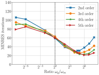
Figure 1: MINRES iterations to relative preconditioned residual tolerance $10^{-8}$ as a function of ratio of constants $\omega_{q}/\omega_{m}$ used in the mass-matrix approximation (18) to the pressure Schur complement (17). Black dotted line denotes the simplest case of $\omega_{q}=\omega_{m}=1$. On the right of this line, $\omega_{m}=1$, while on the left $\omega_{q}=1$.

4.2 Two dimensional robustness test case

Next we run 2d experiments in Firedrake to demonstrate $h$-robustness, to compare exact and inexact solves for the velocity block, and to compare iteration counts with a comparable preconditioner applied to a true BDM discretization [8, 40]. We choose the source term and boundary conditions in eq. 1 such that the exact solution is given by $\boldsymbol{u}=[\sin(\pi x)\sin(\pi y)+2,\cos(\pi x)\cos(\pi y)-1]$ and $p=\sin(\pi x)\cos(\pi y)$ on the unit square $\Omega=(0,1)^{2}$. In table 1 we list the number of iterations MINRES requires to reach a relative preconditioned residual tolerance of $10^{-8}$ for the extended hybridized discretization, using exact and approximate inner solves for $A$, $Q$, and $M$. For approximate inner solvers, both mass matrices, $Q$ and $M$, are approximated by one symmetric Gauss–Seidel relaxation, and $A$ is approximated by four AMG iterations for $k=2$ and ten AMG iterations for $k=4$. We note that both preconditioners (with exact and approximate solves) are optimal in $h$, with only minor degradation in convergence when moving from exact inner solves to approximate inner solves. The modified constant $\omega_{q}>1$ helps in all cases, and is most notable for block-diagonal preconditioning with $k=4$, reducing the iteration count $2.5\times$ compared with $\omega_{q}=1$. In addition, using $\omega_{q}=24$, we again see the super robustness in element order, with lower iteration counts in all cases for $k=4$ compared with $k=2$.

Table 1: Number of MINRES iterations required to reach a relative preconditioned residual tolerance of $10^{-8}$ for preconditioners $\mathbb{P}$ and $\mathbb{P}^{s}$ applied to eq. 11, with preconditioner constants $\omega_{q}=1$ and $\omega_{q}=24$. The number of elements in the mesh is given by $N^{2}\times 2$.

			$\omega_{q}=1$				$\omega_{q}=24$
			Exact		Approx.		Exact		Approx.
$k$	$N$	DOFs	$\mathbb{P}$	$\mathbb{P}^{s}$	$\mathbb{P}$	$\mathbb{P}^{s}$	$\mathbb{P}$	$\mathbb{P}^{s}$	$\mathbb{P}$	$\mathbb{P}^{s}$
2	16	6144	136	60	138	64	64	39	64	43
2	32	24576	134	57	135	60	66	37	66	42
2	64	98304	134	50	134	56	66	34	66	38
2	128	393216	132	46	134	51	66	34	66	39
4	16	24480	160	59	162	65	66	33	66	39
4	32	97600	160	54	162	60	64	32	64	38
4	64	389760	156	54	157	60	62	31	62	37
4	128	1557760	154	53	155	60	61	28	61	34

To compare, table 2 now shows analogous experiments applied to solve eq. 5 without hybridizing. Using similar analysis as in section 3 for the extended system eq. 11 it can be shown that if $R$ is spectrally equivalent to $A$, then $\tilde{\mathbb{P}}={\rm bdiag}(R,M)$ is an optimal preconditioner for eq. 5. Analogous to the hybridized case, we denote the block diagonal and approximate LDU (24) variations $\tilde{\mathbb{P}}$ and $\tilde{\mathbb{P}}^{s}$, respectively. The main difference between solving eq. 5 and eq. 11 is the basis for the velocity space. Indeed for eq. 5 $u\in\mathbb{R}^{n_{u}}$ is the vector of coefficients with respect to the basis for the BDM space ${\rm{\bf BDM}}_{h}^{k}$ while for eq. 11 $u\in\mathbb{R}^{n_{u}}$ is the vector of coefficients with respect to the basis for the DG space $\boldsymbol{V}_{h}^{k}$. As mentioned previously, having the velocity space represented in $H({\rm div})$ is significantly more challenging for black-box solvers such as AMG.

As for the hybridized case, in the preconditioner for eq. 5 we consider two choices of inner approximations: a direct solver applied to $A$ and the pressure mass matrix, or approximate inverses as used in table 1, with one symmetric Gauss–Seidel iteration applied to the mass matrix and $R^{-1}\mathrel{\mathop{\mathchar 58\relax}}=\mathcal{O}(1)$ AMG iterations applied to $A$. From table 2 we note that if a direct solver is used on $A$, then the preconditioners $\tilde{\mathbb{P}}$ and $\tilde{\mathbb{P}}^{s}$ are optimal, and the iteration counts are 1.5–2.5$\times$ less than those observed for the extended system eq. 11 in table 1. However, no convergence was obtained in any cases after switching to AMG to precondition $A$. It should be noted that even with significant parameter tuning, numerical tests indicated that even hundreds of AMG-preconditioned Krylov iterations were unable to make a notable reduction in residual when applied to the $H({\rm div})$-DG discretization of the vector Laplacian. Thus, the fact that block-preconditioning with AMG-approximate inverses did not converge for BDM discretizations (see table 2) makes sense, and is simply because AMG is not an effective preconditioner for the $H({\rm div})$-DG discretization of the vector Laplacian.

Table 2: Number of MINRES iterations required to reach a relative preconditioned residual tolerance of $10^{-8}$ for preconditioners $\tilde{\mathbb{P}}$ and $\tilde{\mathbb{P}}^{s}$ applied to eq. 5. Results are shown for order $k=2$ and $k=4$, both considered with exact inner solves and approximate inner solves. The number of elements in the mesh is given by $N^{2}\times 2$. A $*$ means there was no convergence within 500 iterations.

			Exact		Approx.
$k$	$N$	DOFs	$\tilde{\mathbb{P}}$	$\tilde{\mathbb{P}}^{s}$	$\tilde{\mathbb{P}}$	$\tilde{\mathbb{P}}^{s}$
2	16	5472	32	16	*	*
2	32	21696	35	15	*	*
2	64	86400	33	15	*	*
2	128	344832	33	14	*	*
4	16	16800	37	16	*	*
4	32	66880	37	16	*	*
4	64	266880	37	15	*	*
4	128	1066240	37	15	*	*

4.3 Three dimensional robustness test case

Last, we demonstrate that the proposed preconditioning naturally extends to 3d problems, with even better convergence than the 2d setting. For this we consider a domain $\Omega=(0,1)^{3}$ with the exact solution given by $\boldsymbol{u}=[\pi(\sin(\pi x)\cos(\pi y)-\sin(\pi x)\cos(\pi z)),\pi(\sin(\pi y)\cos(\pi z)-\cos(\pi x)\sin(\pi y)),\pi(\cos(\pi x)\sin(\pi z)-\cos(\pi y)\sin(\pi z))]$ and $p=\sin(\pi x)\cos(\pi y)\sin(2\pi z)$. Here we discretize in MFEM using a 3d unstructured tetrahedral mesh generated with Gmsh [17] and apply the LDU version of block preconditioning, $\mathbb{P}^{s}$, to the extended hybridized system. For approximate solves, 14 AMG iterations are applied (because 3d DG discretizations of diffusion are more challenging to AMG than 2d). We again see the preconditioner is optimal in $h$, super robust in element order (although AMG is not, hence the growth in approximate iteration count between $k=2$ and $k=4$), and the weighting $\omega_{q}=32$ provides a consistent $3\times$ or more reduction in iteration count compared with $\omega_{q}=1$.

Table 3: Number of MINRES iterations required to reach a relative preconditioned residual tolerance of $10^{-8}$ for preconditioner $\mathbb{P}^{s}$ applied to eq. 11 for a 3d problem, using order $k=2$ and $k=4$ elements, and preconditioner constants $\omega_{q}=1$ and $\omega_{q}=32$. $*$ indicates did not finish due to cluster time constraints.

	$\mathbb{P}^{s}$		$\omega_{q}=1$		$\omega_{q}=32$
$k$	Cells	DOFs	Exact	Approx.	Exact	Approx.
2	4192	195712	108	124	34	42
2	33536	1554176	88	104	30	39
2	268288	12387328	70	91	26	39
4	4192	656960	98	156	27	59
4	33536	5226880	84	141	25	54
4	268288	41699840	*	*	23	54

5 Conclusions

Using BDM elements for the velocity field in a DG discretization of the Stokes equations results in a velocity field that is exactly divergence-free. As a consequence, it can be shown that the discretization is pressure-robust. Unfortunately, “black-box” solvers perform poorly on discretizations using BDM elements and specialized (custom) preconditioners are required for the efficient solution of such systems.

As an alternative, one may hybridize the discretization, so that the velocity lives in a “friendlier” standard $L^{2}$-DG space. Typically, hybridization allows one to eliminate all element degrees-of-freedom and to obtain a global system for a Lagrange multiplier only. However, since the BDM element is a nonconforming element for the Stokes problem, elimination of element degrees-of-freedom is not possible. Nevertheless, as we have shown in this manuscript, the extended hybridized system is much better suited for “black-box” solvers. We have presented an optimal preconditioner for the hybridized system of which each component is directly available in most linear algebra packages. The preconditioner is robust in $h$, super robust in element order, and naturally effective in 2d and 3d (in fact, iteration counts are lower in 3d). Moreover, no custom solvers are necessary.

Last, we point out that the hybridization extends naturally to arbitrary Reynolds Navier–Stokes problems, and there exist fast solvers for high-Reynolds velocity fields of the extended hybridized system [29, 30]. Future work will focus on developing block preconditioning techniques for the extended hybridized system of Navier–Stokes.

References

- [1] D. N. Arnold, R. S. Falk, and R. Winther. Multigrid in and . Numer. Math., 85:197–217, 2000.
- [2] Douglas N Arnold and Franco Brezzi. Mixed and nonconforming finite element methods: implementation, postprocessing and error estimates. ESAIM: Mathematical Modelling and Numerical Analysis, 19(1):7–32, 1985.
- [3] Satish Balay, Shrirang Abhyankar, Mark F. Adams, Jed Brown, Peter Brune, Kris Buschelman, Lisandro Dalcin, Victor Eijkhout, William D. Gropp, Dmitry Karpeyev, Dinesh Kaushik, Matthew G. Knepley, Dave A. May, Lois Curfman McInnes, Richard Tran Mills, Todd Munson, Karl Rupp, Patrick Sanan, Barry F. Smith, Stefano Zampini, Hong Zhang, and Hong Zhang. PETSc users manual. Technical Report ANL-95/11 - Revision 3.11, Argonne National Laboratory, 2019.
- [4] Satish Balay, Shrirang Abhyankar, Mark F. Adams, Jed Brown, Peter Brune, Kris Buschelman, Lisandro Dalcin, Victor Eijkhout, William D. Gropp, Dinesh Kaushik, Matthew G. Knepley, Lois Curfman McInnes, Karl Rupp, Barry F. Smith, Stefano Zampini, Hong Zhang, and Hong Zhang. PETSc Web page. http://www.mcs.anl.gov/petsc, 2016.
- [5] Franco Brezzi, Jim Douglas, and L Donatella Marini. Two families of mixed finite elements for second order elliptic problems. Numerische Mathematik, 47(2):217–235, 1985.
- [6] Peter N Brown, Robert D Falgout, and Jim E Jones. Semicoarsening multigrid on distributed memory machines. SIAM Journal on Scientific Computing, 21(5):1823–1834, 2000.
- [7] B. Cockburn, G. Kanschat, and D. Schötzau. A locally conservative LDG method for the incompressible Navier–Stokes equations. Math. Comp., 74(251):1067–1095, 2004.
- [8] B. Cockburn, G. Kanschat, and D. Schötzau. A note on discontinuous Galerkin divergence-free solutions of the Navier–Stokes equations. J. Sci. Comput., 31(1/2):61–73, 2007.
- [9] B. Cockburn and F. J. Sayas. Divergence-conforming HDG methods for Stokes flows. Math. Comp., 83:1571–1598, 2014.
- [10] Lisandro D. Dalcin, Rodrigo R. Paz, Pablo A. Kler, and Alejandro Cosimo. Parallel distributed computing using Python. Advances in Water Resources, 34(9):1124–1139, 2011. New Computational Methods and Software Tools.
- [11] D. A. Di Pietro and A. Ern. Mathematical Aspects of Discontinuous Galerkin Methods, volume 69 of Mathématiques et Applications. Springer–Verlag Berlin Heidelberg, 2012.
- [12] Blanca Ayuso de Dios, Franco Brezzi, L. Donatella Marini, Jinchao Xu, and Ludmil Zikatanov. A Simple Preconditioner for a Discontinuous Galerkin Method for the Stokes Problem. Journal of Scientific Computing, 58(3):517–547, 2014.
- [13] V. Dobrev, T. Kolev, C. S. Lee, V. Tomov, and P. S. Vassilevski. Algebraic hybridization and static condensation with application to scalable preconditioning. SIAM J. Sci. Comput., 41(3):B425–B447, 2019.
- [14] V. Dobrev, R. D. Lazarov, P. S. Vassilevski, and L. T. Zikatanov. Two-level preconditioning of discontinuous Galerkin approximations of second-order elliptic equations. Numer. Linear Algebra Appl., 13:753–770, 2006.
- [15] V. A. Dobrev, T. V. Kolev, et al. MFEM: Modular finite element methods. http://mfem.org, 2020.
- [16] Robert D Falgout and Ulrike Meier Yang. hypre: A library of high performance preconditioners. In International Conference on Computational Science, pages 632–641. Springer, 2002.
- [17] C. Geuzaine and J.-F. Remacle. Gmsh: a three-dimensional finite element mesh generator with built-in pre- and post-processing facilities. International Journal for Numerical Methods in Engineering, 79(11):1309–1331, 2009.
- [18] Chen Greif, Dan Li, Dominik Schötzau, and Xiaoxi Wei. A mixed finite element method with exactly divergence-free velocities for incompressible magnetohydrodynamics. Computer Methods in Applied Mechanics and Engineering, 199(45-48):2840–2855, 2010.
- [19] Johnny Guzmán, Chi-Wang Shu, and Filánder A Sequeira. H(div) conforming and DG methods for incompressible Euler’s equations. IMA Journal of Numerical Analysis, 37(4):1733–1771, 2017.
- [20] Ralf Hiptmair and Jinchao Xu. Nodal Auxiliary Space Preconditioning in H(curl) and H(div) Spaces. SIAM Journal on Numerical Analysis, 45(6):2483–2509, 2007.
- [21] Qingguo Hong, Johannes Kraus, Jinchao Xu, and Ludmil Zikatanov. A robust multigrid method for discontinuous Galerkin discretizations of Stokes and linear elasticity equations. Numerische Mathematik, 132(1):23–49, 2016.
- [22] J. S. Howell and N. J. Walkington. Inf-sup conditions for twofold saddle point problems. Numer. Math., 118:663–693, 2011.
- [23] V. John, A. Linke, C. Merdon, M. Neilan, and L. G. Rebholz. On the divergence constraint in mixed finite element methods for incompressible flows. SIAM Rev., 59(3):492–544, 2017.
- [24] Guido Kanschat and Youli Mao. Multigrid methods for Hdiv-conforming discontinuous Galerkin methods for the Stokes equations. Journal of Numerical Mathematics, 23(1):51–66, 2015.
- [25] Guido Kanschat and Youli Mao. Multiplicative Overlapping Schwarz Smoothers for Hdiv-Conforming Discontinuous Galerkin Methods for the Stokes Problem. In Domain Decomposition Methods in Science and Engineering XXII, Lecture Notes in Computational Science and Engineering, pages 285–292, 2016.
- [26] Guido Kanschat and Béatrice Riviere. A strongly conservative finite element method for the coupling of Stokes and Darcy flow. Journal of Computational Physics, 229(17):5933–5943, 2010.
- [27] C. H. Lee and P. S. Vassilevski. Parallel solver for (div) problems using hybridization and AMG. In Domain Decomposition Methods in Science and Engineering XXIII, pages 69–80. Springer, 2017.
- [28] C. Lehrenfeld and J. Schöberl. High order exactly divergence-free hybrid discontinuous Galerkin methods for unsteady incompressible flows. Comput. Methods Appl. Mech. Engrg., 307:339–361, 2016.
- [29] Thomas A Manteuffel, Steffen Münzenmaier, John Ruge, and Ben Southworth. Nonsymmetric reduction-based algebraic multigrid. SIAM Journal on Scientific Computing, 41(5):S242–S268, 2019.
- [30] Thomas A Manteuffel, John Ruge, and Ben S Southworth. Nonsymmetric algebraic multigrid based on local approximate ideal restriction (AIR). SIAM Journal on Scientific Computing, 40(6):A4105–A4130, 2018.
- [31] Ricardo Oyarzúa, Tong Qin, and Dominik Schötzau. An exactly divergence-free finite element method for a generalized Boussinesq problem. IMA journal of numerical analysis, 34(3):1104–1135, 2014.
- [32] Will Pazner. Efficient low-order refined preconditioners for high-order matrix-free continuous and discontinuous galerkin methods. SIAM Journal on Scientific Computing, 42(5):A3055–A3083, 2020.
- [33] J. Pestana and A. J. Wathen. Natural preconditioning and iterative methods for saddle point systems. SIAM Rev., 57(1):71–91, 2015.
- [34] Florian Rathgeber, David A Ham, Lawrence Mitchell, Michael Lange, Fabio Luporini, Andrew TT McRae, Gheorghe-Teodor Bercea, Graham R Markall, and Paul HJ Kelly. Firedrake: automating the finite element method by composing abstractions. ACM Transactions on Mathematical Software (TOMS), 43(3):1–27, 2016.
- [35] Pierre-Arnaud Raviart and Jean-Marie Thomas. A mixed finite element method for 2-nd order elliptic problems. In Mathematical aspects of finite element methods, pages 292–315. 1977.
- [36] S. Rhebergen and G. Wells. A hybridizable discontinuous Galerkin method for the Navier–Stokes equations with pointwise divergence-free velocity field. J. Sci. Comput., 76(3):1484–1501, 2018.
- [37] S. Rhebergen and G. N. Wells. Preconditioning of a hybridized discontinuous Galerkin finite element method for the Stokes equations. J. Sci. Comput., 77(3):1936–1952, 2018.
- [38] Thomas W Roberts, David Sidilkover, and RC Swanson. Textbook multigrid efficiency for the steady euler equations. 2004.
- [39] Klaus Stüben. A review of algebraic multigrid. Numerical Analysis: Historical Developments in the 20th Century, pages 331–359, 2001.
- [40] J. Wang and X. Ye. New finite element methods in computational fluid dynamics by H(div) elements. SIAM J. Numer. Anal., 45:1269–1286, 2007.