Unified dark sectors in scalar-torsion theories of gravity

Abstract

We present a unified description of the matter and dark energy epochs, using a class of scalar-torsion theories. We provide a Hamiltonian description, and by applying Noether’s theorem and by requiring the field equations to admit linear-in-momentum conservation laws we obtain two specific classes of scalar-field potentials. We extract analytic solutions and we perform a detailed dynamical analysis. We show that the system possesses critical points that correspond to scaling solutions in which the effective, total equation-of-state parameter is close to zero, and points in which it is equal to the cosmological constant value $-1$. Therefore, during evolution, the Universe remains for sufficiently long times at the epoch corresponding to dust-matter domination, while at later times it enters the accelerated epoch and it eventually results in the de Sitter phase. Finally, in contrast to other unified scenarios, such as Chaplygin gas-based models as well as Horndeski-based constructions, the present scenario is free from instabilities and pathologies at the perturbative level.

I Introduction

According to detailed observations of different origins, the Universe has entered a period of accelerated expansion in the recent cosmological past. The simplest explanation is the cosmological constant, nevertheless, the corresponding problem, as well as the possibility of a dynamical nature, led to two main classes for its description. The first is to maintain general relativity and introduce the concept of dark energy, which accounts for all forms of new, exotic sectors that can be sources of acceleration Copeland:2006wr ; Cai:2009zp . The second is to attribute the new degrees of freedom to modifications of the gravitational interaction CANTATA:2021ktz ; Capozziello:2011et ; Nojiri:2010wj , namely to extended theories that have general relativity as a limit but which in general have a richer structure. Additionally, there are cumulative pieces of evidence that most of the universe’s matter content is in the form of Cold Dark Matter (CDM) Liddle:1993fq ; Planck:2018vyg ; Abdalla:2022yfr . Although most cosmologists believe that dark matter should correspond to some particle beyond the Standard Model, the fact that it has not been directly detected in the accelerators led to the investigation of many models in which dark matter can have, partially or completely, gravitational origin Nojiri:2006gh ; Famaey:2011kh ; Sebastiani:2016ras ; Addazi:2021xuf . Modified theories of gravity may arise by extending the Einstein-Hilbert action in a suitable way, such as in $F(R)$ DeFelice:2010aj and $F(G)$ Nojiri:2005jg ; DeFelice:2008wz gravity, in Lovelock construction Lovelock:1971yv ; Deruelle:1989fj , in Horndeski gravity Horndeski:1974wa , in generalized galileon theories DeFelice:2010nf ; Deffayet:2011gz , etc. Nevertheless, one can construct gravitational modifications starting from the equivalent torsional formulation of gravity Pereira ; Maluf:2013gaa and build theories such as $F(T)$ gravity Cai:2015emx ; Ferraro:2006jd ; Linder:2010py , $F(T,T_{G})$ gravity Kofinas:2014owa , $F(T,B)$ gravity Bahamonde:2015zma , etc. In this framework one can also introduce scalar fields, i.e. constructing scalar-torsion theories Geng:2011aj , allowing for non-minimal Geng:2011aj ; Geng:2011ka ; Gonzalez-Espinoza:2020jss ; Paliathanasis:2021nqa ; Gonzalez-Espinoza:2021qnv ; Toporensky:2021poc or derivative Kofinas:2015hla couplings with torsion, or more general constructions Geng:2012vtr ; Skugoreva:2014ena ; Jarv:2015odu ; Skugoreva:2016bck ; Hohmann:2018rwf ; Hohmann:2018vle ; Hohmann:2018ijr ; Hohmann:2018dqh ; Emtsova:2019qsl , than can even be the teleparallel version of Horndeski theories Bahamonde:2019shr ; Bahamonde:2020cfv ; Bahamonde:2021dqn ; Bernardo:2021izq .

On the other hand, a large amount of research has been devoted to obtaining a unified description of the Universe, namely introducing a single component that can behave as dust matter at early and intermediate times, and as the acceleration source at late times. The typical example of such classes is the Chaplygin gas cosmology Bilic:2001cg ; Bento:2002ps ; Dev:2002qa , in which one introduces by hand an exotic fluid with a peculiar equation-of-state parameter, that is close to zero at early times, it is progressively increasing, acquiring a value around $-0.7$ today, as it is required by the observed total equation of state of the Universe at present, and finally in the future results to $-1$, i.e to de Sitter phase. Similarly, one can apply Generalized Galileons/Horndeski theories Horndeski:1974wa ; DeFelice:2010nf ; Deffayet:2011gz and require the extra scalar field to describe both the matter and dark-energy sectors in a unified way Koutsoumbas:2017fxp . However, although the generalized Chaplygin gas can indeed describe the evolution of the Universe at the background level Bento:2002yx ; Bento:2005un , it may lead to perturbative instabilities Sandvik:2002jz , which then require the introduction of extra mechanisms to cure them, such as small entropy perturbations Farooq:2010xm ; Gorini:2007ta or baryonic matter that can improve the behavior of the matter power spectrum Debnath:2004cd ; BouhmadiLopez:2004mp ; Setare:2007mp . Similarly, in Horndeski-based theories of dark-sector unification, perturbative instabilities related to the sound-speed square may arise too Koutsoumbas:2017fxp ; Babichev:2007dw ; Deffayet:2010qz ; Easson:2013bda .

In this work, we want to present a unified description of the matter and dark energy epochs, using not a peculiar, exotic fluid, but a class of scalar-torsion theories. Although such constructions are usually applied for the description of only the dark energy sector, in this work, we apply the Noether symmetry approach to constructing suitably models which give rise to an effective cosmic fluid whose equation-of-state behaves as the pressureless matter at early times, and as dark energy at late ones. As we will see, the unified description can indeed be obtained, and this is achieved without the presence of instabilities at the perturbative level.

The plan of the work is the following. In Section II we briefly review the scalar-torsion theories of gravity and in Section III we present their Hamiltonian description, focusing on the conservation laws. Then, in Section IV we extract analytic solutions, investigating the asymptotic dynamics by applying the dynamical system analysis. Finally, in Section V we discuss our results and present our conclusions.

II Scalar-torsion theories

In the torsional formulation of gravity one uses the tetrad fields ${\mathbf{e}_{A}(x^{\mu})}$, which form an orthonormal basis at a manifold point $x^{\mu}$. In a coordinate basis they are expressed as $\mathbf{e}_{A}=e^{\mu}_{A}\partial_{\mu}$, and the spacetime metric is

$$g_{\mu\nu}(x)=\eta_{AB}\,e^{A}_{\mu}(x)\,e^{B}_{\nu}(x),$$ (1)

with $\eta_{AB}={\rm diag}(-1,1,1,1)$ and where Greek and Latin indices are used to denote coordinate and tangent space respectively. Moreover, one introduces the Weitzenböck connection $\overset{\mathbf{w}}{\Gamma}^{\lambda}_{\nu\mu}\equiv e^{\lambda}_{A}\>\partial_{\mu}e^{A}_{\nu}$, and hence the corresponding torsion tensor reads as

$${T}^{\lambda}_{\>\mu\nu}\equiv\overset{\mathbf{w}}{\Gamma}^{\lambda}_{\nu\mu}-\overset{\mathbf{w}}{\Gamma}^{\lambda}_{\mu\nu}=e^{\lambda}_{A}\>(\partial_{\mu}e^{A}_{\nu}-\partial_{\nu}e^{A}_{\mu}).$$ (2)

On can construct the torsion scalar by its contraction as

$$T\equiv\frac{1}{4}T^{\rho\mu\nu}T_{\rho\mu\nu}+\frac{1}{2}T^{\rho\mu\nu}T_{\nu\mu\rho}-T_{\rho\mu}^{\ \ \rho}T_{\ \ \ \nu}^{\nu\mu},$$ (3)

which is then used as the Lagrangian of teleparallel gravity. In particular, writing the action

$$S=\frac{1}{16\pi G}\int d^{4}xeT,$$ (4)

with $e=\text{det}(e_{\mu}^{A})=\sqrt{-g}$ and $G$ the gravitational constant, and performing variation in terms of the tetrads leads to the same equations of general relativity, and that is why the theory at hand is named teleparallel equivalent of general relativity (TEGR).

One can add a scalar field $\phi$ to the above framework, resulting to the scalar-torsion theories of gravity. As it has been extensively discussed, although TEGR is equivalent with general relativity, $f(T)$ is different than $f(R)$ gravity, and similarly scalar-torsion theories are in general different than scalar-tensor (i.e. scalar-curvature) gravity, due to the different structure of curvature and torsion tensors Cai:2015emx . The simplest scalar-torsion action is Geng:2011aj

$$S=\int d^{4}xe\left[\left(1+\xi\phi^{2}\right)T+\partial_{\mu}\phi\partial^{\mu}\phi-2V\left(\phi\right)\right],$$ (5)

with $V(\phi)$ the potential of the scalar field, $\xi$ the coupling parameter, and where for simplicity we use units where $8\pi G=1$.

We consider a spatially flat Friedmann–Lemaître–Robertson–Walker (FLRW) background metric with line element

$$ds^{2}=-dt^{2}+a^{2}\left(t\right)\left(dx^{2}+dy^{2}+dz^{2}\right).$$ (6)

Hence, the two Friedmann equations become

$$3H^{2} =\rho_{\phi},$$ (7)

$$-2\dot{H}-3H^{2} =P_{\phi},$$ (8)

with $H=\frac{\dot{a}}{a}$ the Hubble function and where the effective energy density and pressure for the scalar field are written as Geng:2011aj

$$\rho_{\phi} =\frac{1}{2}\dot{\phi}^{2}+V\left(\phi\right)-3\xi H^{2}\phi^{2},$$ (9)

$$P_{\phi} =\frac{1}{2}\dot{\phi}^{2}-V\left(\phi\right)+4\xi H\phi\dot{\phi}+\xi\left(2\dot{H}+3H^{2}\right)\phi^{2}.$$ (10)

Additionally, variation of (5) leads to the Klein-Gordon equation

$$\ddot{\phi}+3H\dot{\phi}+6\xi H\phi+V_{,\phi}\left(\phi\right)=0,$$ (11)

which can be re-written equivalently as

$$\dot{\rho}_{\phi}+3H\left(\rho_{\phi}+P_{\phi}\right)=0.$$ (12)

Finally, note that we can introduce the equation-of-sate parameter for the scalar field as

$$w_{eff}\equiv\frac{P_{\phi}}{\rho_{\phi}}.$$ (13)

We close this section by presenting the minisuperspace description of the above theory. In particular, we start by re-writing the FLRW line element adding the lapse function, namely

$$ds^{2}=-N^{2}\left(t\right)dt^{2}+a^{2}\left(t\right)\left(dx^{2}+dy^{2}+dz^{2}\right).$$ (14)

Then, the field equations follow from the variation of the point-like Lagrangian

$$\mathcal{L}\left(N,a,\dot{a},\phi,\dot{\phi}\right)$$

$$=\frac{1}{N}\left[-3\left(1+\xi\phi^{2}\right)a\dot{a}^{2}+\frac{1}{2}a^{3}\dot{\phi}^{2}\right]-Na^{3}V\left(\phi\right).$$ (15)

Specifically, the first Friedmann (constraint) equation (7) is obtained from the Euler-Lagrange equation $\frac{\partial\mathcal{L}}{\partial N}=0$, while the second Friedmann equation (8) is provided by the Euler-Lagrange equations with respect to the scale factor $a$, $\frac{d}{dt}\frac{\partial\mathcal{L}}{\partial\dot{a}}-\frac{\partial\mathcal{L}}{\partial a}=0$. Finally, the scalar field equation arises from $\frac{d}{dt}\frac{\partial\mathcal{L}}{\partial\dot{\phi}}-\frac{\partial\mathcal{L}}{\partial\phi}=0$. As usual, in all the above equations one can set $N\left(t\right)=1$ after the derivations.

III Hamiltonian description and conservation laws

We continue by introducing a re-scaled scalar field $\psi\left(t\right)$ defined as $\phi=\frac{1}{\sqrt{\xi}}\sinh\left(\sqrt{\xi}\psi\right)$. In the new variables, the point-like Lagrangian (15) becomes

$$\mathcal{L}\left(N,a,\dot{a},\psi,\dot{\psi}\right)$$

$$=\frac{1}{N}\cosh^{2}\left(\sqrt{\xi}\psi\right)\left(-3a\dot{a}^{2}+\frac{1}{2}a^{3}\dot{\psi}^{2}\right)-a^{3}NV\left(\psi\right).$$ (16)

Hence, the field equations become

$$\cosh^{2}\left(\sqrt{\xi}\psi\right)\left(-3H^{2}+\frac{1}{2}\dot{\psi}^{2}\right)+V\left(\psi\right)=0,$$ (17)

$$2\dot{H}+3H^{2}+\frac{1}{2}\dot{\psi}^{2}+4\sqrt{\xi}H\tanh\left(\sqrt{\xi}\psi\right)\dot{\psi}-\frac{V\left(\psi\right)}{\cosh^{2}\left(\sqrt{\xi}\psi\right)}=0,$$ (18)

$$\ddot{\psi}+3H\dot{\psi}+\sqrt{\xi}\tanh\left(\sqrt{\xi}\psi\right)\left(\dot{\psi}^{2}+6H^{2}\right)+\frac{V_{,\psi}\left(\psi\right)}{\cosh^{2}\left(\sqrt{\xi}\psi\right)}=0,$$ (19)

where $H=\dot{a}/(aN)$, and we set $N\left(t\right)=1$ in the end. Therefore, the energy density and pressure for the scalar field are defined as

$$\rho_{\psi}=\frac{1}{2}\dot{\psi}^{2}+\frac{V\left(\psi\right)}{\cosh^{2}\left(\sqrt{\xi}\psi\right)},$$ (20)

$$P_{\psi}=\frac{1}{2}\dot{\psi}^{2}+4\sqrt{\xi}H\tanh\left(\sqrt{\xi}\psi\right)\dot{\psi}-\frac{V\left(\psi\right)}{\cosh^{2}\left(\sqrt{\xi}\psi\right)},$$ (21)

while the equation-of-sate parameter becomes

$$w_{eff}\equiv\frac{P_{\psi}}{\rho_{\psi}}.$$ (22)

Since $\psi$ is just the re-scaled $\phi$, the physical properties of the scenario are the same as the initial scalar-torsion theory.

The cosmological equations (17)-(20) form an autonomous dynamical system described by the point-like Lagrangian (16), where equation (17) can be seen as the energy conservation law for the Euler-Lagrange equations (18), (19). For the Lagrangian function (16) we define the generalized momenta by $p_{i}=\frac{\partial{\mathcal{L}}}{\partial{\dot{q}}^{i}}$, where $q^{i}\in\{a,\psi\}$, $p_{i}\in\{p_{a},p_{\psi}\}$, namely

$$p_{a} \equiv-6a\frac{\cosh^{2}\left(\sqrt{\xi}\psi\right)}{N}\dot{a},$$ (23)

$$p_{\psi} \equiv\frac{\cosh^{2}\left(\sqrt{\xi}\psi\right)}{N}a^{3}\dot{\psi}.$$ (24)

Hence, we can introduce the Hamiltonian function $\mathcal{H}=p_{a}\dot{a}+p_{\psi}\dot{\psi}-\mathcal{L}$, which is written as

$$\mathcal{H}=\frac{N}{\cosh^{2}\left(\sqrt{\xi}\psi\right)}\left(\frac{p_{\psi}^{2}}{2a^{3}}-\frac{p_{a}^{2}}{12a}\right)+a^{3}NV\left(\psi\right).$$ (25)

Note that $d{\mathcal{H}}/dt=0$, and as expected the first Friedmann (constraint) equation (17) becomes $\mathcal{H}\left(N,a,\psi,p_{a},p_{\psi}\right)\equiv 0$. Thus, we have the evolution Eqs. for $(\dot{a},\dot{\psi})$ as given by (23), (24). Additionally, Hamilton’s equations ${\dot{p}}_{i}=-{\frac{\partial{\mathcal{H}}}{\partial q^{i}}}$, where $q^{i}\in\{a,\psi\}$, $p_{i}\in\{p_{a},p_{\psi}\}$, lead to

$$\frac{1}{N}\dot{p}_{a}=\frac{1}{\cosh^{2}\left(\sqrt{\xi}\psi\right)}\left(\frac{3}{2}\frac{p_{\psi}^{2}}{a^{4}}-\frac{p_{a}^{2}}{12a^{2}}\right)-3a^{2}V(\psi),$$ (26)

$$\frac{1}{N}\dot{p}_{\psi}=\frac{\sqrt{\xi}\tanh\left(\sqrt{\xi}\psi\right)}{\cosh^{2}\left(\sqrt{\xi}\psi\right)}\left(\frac{p_{\psi}^{2}}{a^{3}}-\frac{p_{a}^{2}}{6a}\right)-a^{3}V_{,\psi}(\psi).$$ (27)

To proceed with the derivation of analytic solutions for the Hamiltonian system (23), (24), (26), (27), we have to investigate the integrability properties of the system. Indeed, the Hamiltonian function (25) is a conservation law for the dynamical system. Thus, we must find the potential functions $V(\psi)$ for which the dynamical system admits additional conservation laws.

We are interested in studying the existence of conservation laws in the field equations that are linear in momentum. Specifically, we apply Noether’s theorem to constraint the function $V(\psi)$, for the field equations to possess Noetherian first integrals. This approach has been widely applied in the literature, with many interesting results Rosquist ; Cotsakis:1998zk ; Vakili:2008ea ; Capozziello:2009te ; Zhang:2009mm ; MohseniSadjadi:2012brg ; Vakili:2011uz ; Atazadeh:2011aa ; Dong:2013rea ; Christodoulakis:2014wba ; Terzis:2014cra ; Dimakis:2013oza ; Dimakis:2017kwx ; Paliathanasis:2014zxa ; Papagiannopoulos:2016dqw ; Paliathanasis:2011jq ; Paliathanasis:2015aos . Concerning teleparallel and torsional gravity, Noether’s symmetry approach was applied in Basilakos:2013rua ; Paliathanasis:2014iva ; Karpathopoulos:2017arc ; Capozziello:2016eaz ; Bahamonde:2016grb . Moreover, as has been discussed in Basilakos:2011rx , the application of Noether’s conditions for the constraint of the scalar field potential is a geometric selection rule since there exists a relation between Noether symmetries and the collineations of the minisuperspace for the field equations. In the following, we omit the calculations for the derivation of Noether symmetries and the approach that we follow can be found in detail in Tsamparlis:2018nyo .

In summary, we find two non-zero scalar field potentials, for which the field equations admit linear-in-momentum conservation laws, and we separately present them in the following subsections.

III.1 Potential $V_{A}\left(\phi\right)=V_{0}\cosh^{-2}\left(\sqrt{\xi}\psi\right)$

According to the Noether analysis, the first potential function that we extract is $V_{A}\left(\phi\right)=V_{0}\cosh^{-2}\left(\sqrt{\xi}\psi\right)$. Thus, we find that the field equations admit the Noether symmetries which provide the linear first integrals

$$\!\!\!\!\!\!\!\!\!\!\!\!\!\!\!X^{1}=\frac{1}{a^{3}}\!\left[a\cosh\!\left(\!\frac{\sqrt{6}}{2}\psi\!\right)\partial_{a}-\sqrt{6}\sinh\!\left(\!\frac{\sqrt{6}}{2}\psi\!\right)\partial_{\psi}\!\right]\!,$$ (28)

$$\!\!\!\!\!\!\!\!\!\!\!\!\!\!\!X^{2}=-\frac{1}{a^{3}}\!\left[a\sinh\!\left(\!\frac{\sqrt{6}}{2}\psi\!\right)\partial_{a}+\sqrt{6}\cosh\!\left(\!\frac{\sqrt{6}}{2}\psi\!\right)\partial_{\psi}\!\right]\!,$$ (29)

$$\!\!\!\!\!\!\!\!\!\!\!\!\!\!X^{3}=\partial_{\psi}~{}.$$ (30)

These Noether symmetries form the three-dimensional Lie algebra $\left\{X^{1},X^{2},X^{3}\right\}$, with nonzero commutators $\left[X^{1},X^{3}\right]=\sqrt{6}X^{2},~{}\left[X^{2},X^{3}\right]=-\sqrt{6}X^{1}$. Moreover, the corresponding linear-in-momentum conservation laws are derived as

$$I_{1}\left(a,\psi,p_{a},p_{\psi}\right)$$

$$=\frac{1}{a^{3}}\left[a\cosh\left(\frac{\sqrt{6}}{2}\psi\right)p_{a}-\sqrt{6}\sinh\left(\frac{\sqrt{6}}{2}\psi\right)p_{\psi}\right],$$ (31)

$$I_{2}\left(a,\psi,p_{a},p_{\psi}\right)$$

$$=\frac{1}{a^{3}}\left[a\sinh\left(\frac{\sqrt{6}}{2}\psi\right)p_{a}-\sqrt{6}\cosh\left(\frac{\sqrt{6}}{2}\psi\right)p_{\psi}\right],$$ (32)

$$I_{3}\left(a,\psi,p_{a},p_{\psi}\right)=p_{\psi}.$$ (33)

For these functions we calculate $\left\{I_{A},\mathcal{H}\right\}\simeq\mathcal{H}$, which becomes $\left\{I_{A},\mathcal{H}\right\}\simeq 0$, since the dynamical system is constrained Christodoulakis:2014wba ; Terzis:2014cra ; Dimakis:2013oza .

III.2 Potential $V_{B}\left(\phi\right)=V_{0}e^{-\lambda\psi}\cosh^{-2}\left(\sqrt{\xi}\psi\right)$

The second potential function that we extract, in which the field equations admit a linear first integral, is $V_{B}\left(\phi\right)=V_{0}e^{-\lambda\psi}\cosh^{-2}\left(\sqrt{\xi}\psi\right)$, which in the limit $\lambda=0$ recovers the potential of the previous subsection. The Noether symmetries of the field equations are

$$Y^{1} =\frac{1}{\sqrt{6}}a^{\frac{3}{\sqrt{6}}\lambda-3}e^{-\frac{1}{2}\left(\sqrt{6}-\lambda\right)\psi}\left(a\partial_{a}+\partial_{\psi}\right),$$ (34)

$$Y^{2} =-\frac{1}{\sqrt{6}}a^{-\frac{3}{\sqrt{6}}\lambda-3}e^{\frac{1}{2}\left(\sqrt{6}+\lambda\right)\psi}\left(a\partial_{a}-\partial_{\psi}\right),~{}$$ (35)

$$Y^{3} =a\lambda\partial_{a}+\partial_{\psi}~{}.$$ (36)

Furthermore, the nonzero commutators of the Noether symmetries $\left\{Y^{1},Y^{2},Y^{3}\right\}$ are $\left[Y^{1},Y^{3}\right]=\sqrt{6}\left(\frac{\lambda^{2}}{6}-1\right)Y^{2}$ and $\left[Y^{2},Y^{3}\right]=-\sqrt{6}\left(\frac{\lambda^{2}}{6}-1\right)Y^{1}$. Therefore, the corresponding Noetherian first integrals are

$$\Phi_{1}\left(a,\psi,p_{a},p_{\psi}\right) =\frac{1}{\sqrt{6}}a^{\frac{3}{\sqrt{6}}\lambda-3}e^{-\frac{1}{2}\left(\sqrt{6}-\lambda\right)\psi}\left(ap_{a}+p_{\psi}\right),$$ (37)

$$\Phi_{2}\left(a,\psi,p_{a},p_{\psi}\right) =-\frac{1}{\sqrt{6}}a^{-\frac{3}{\sqrt{6}}\lambda-3}e^{\frac{1}{2}\left(\sqrt{6}+\lambda\right)\psi}\left(ap_{a}-p_{\psi}\right),$$ (38)

$$\Phi_{3}\left(a,\psi,p_{a},p_{\psi}\right) =a\lambda p_{a}+6p_{\psi}~{}.$$ (39)

IV Analytic solutions and asymptotic dynamics

In this section, we will extract analytic solutions for the Liouville integrable scalar-field potentials. It is important to mention here that these potential functions admit more conservation laws from the degrees of freedom of the Hamiltonian system, namely the scalar field potentials are super-integrable. As we observe, for the above two scalar-field potentials the cosmological field equations admit three vector fields as additional Noether symmetries elements, for each potential, which forms the same algebra. Consequently, potentials $V_{A}\left(\phi\right)$ and $V_{B}\left(\phi\right)$ admit as Noether symmetries the same Lie algebra but in a different representation.

The solution approach that we shall follow is summarized in the following steps Tsamparlis:2018nyo : first, we define the normal coordinates; then, as a second step, we apply the canonical transformations and we write the Hamilton-Jacobi equation; finally, from the action arising from the Hamilton-Jacobi equation we reduce the field equations into a system of two first-order differential equations. In general, this is considered to be the general solution for the scenario at hand. Nevertheless, if it is feasible we will also provide a closed-form solution.

IV.1 Potential $V_{A}\left(\phi\right)=V_{0}\cosh^{-2}\left(\sqrt{\xi}\psi\right)$

For the scalar field potential $V_{A}\left(\phi\right)$,  Noether symmetry $X^{3}$ is already in normal coordinates. Hence, from (25) and (33) we result to the Hamilton-Jacobi equations

$$\left\{\frac{1}{2a^{3}}\left[\frac{\partial S\left(a,\psi\right)}{\partial\psi}\right]^{2}-\frac{1}{12a}\left(\frac{\partial S\left(a,\psi\right)}{\partial a}\right)^{2}\right\}+a^{3}=0~{},$$ (40)

$$\left[\frac{\partial S\left(a,\psi\right)}{\partial\psi}\right]=I_{3}\text{~{}}.$$ (41)

Therefore, the corresponding action is calculated as

$$S\left(a,\psi\right)=I_{3}\psi+\int\sqrt{6I_{3}^{2}a^{-2}+12a^{4}}da+S_{0},$$ (42)

which implies that the field equations are reduced to the following system

$$\frac{1}{N}\dot{a} =-\frac{6\sqrt{6I_{3}^{2}a^{-4}+12a^{2}}}{\cosh^{2}\left(\sqrt{\xi}\psi\right)}$$ (43)

$$\frac{1}{N}\dot{\psi} =\frac{I_{3}}{\cosh^{2}\left(\sqrt{\xi}\psi\right)}.$$ (44)

The solution of the above equations is expressed in terms of the elliptic integral

$$\psi\left(a\right)=-\frac{I_{3}}{6}\int\frac{da}{\sqrt{6I_{3}^{2}a^{-4}+12a^{2}}}.$$ (45)

For small values of $a$, we derive $\psi\left(a\right)\simeq\psi_{0}a^{3}$, and thus $\frac{1}{N}\frac{\dot{a}}{a}\simeq-6\sqrt{6I_{3}^{2}a^{-6}+12}\left(1-\sqrt{\xi}\psi_{0}a^{6}\right)$, which leads to

$$H\left(a\right)=\frac{1}{N}\frac{\dot{a}}{a}$$

$$\simeq\sqrt{6I_{3}^{2}a^{-6}+12}\left(1-\sqrt{\xi}\psi_{0}a^{6}\right)\simeq\sqrt{6I_{3}^{2}a^{-6}}.$$ (46)

As we deduce, the early-time solution is approximated by that of a stiff fluid. On the other hand, for large values of the scale factor we have $\psi\left(a\right)\simeq\psi_{0}\ln a,~{}\psi_{0}\simeq I_{3}$, which implies that

$$H\left(a\right)=\frac{1}{N}\frac{\dot{a}}{a}\simeq a^{-2\sqrt{\xi}\psi_{0}}\text{. }$$ (47)

Hence, the late-time solution is that of an ideal gas.

IV.2 Potential $V_{B}\left(\phi\right)=V_{0}e^{-\lambda\psi}\cosh^{-2}\left(\sqrt{\xi}\psi\right)$

For the potential $V_{B}\left(\phi\right)$ we apply the canonical transformation $a=\frac{1}{6}\left(\lambda\psi-u\right)$, and the point-like Lagrangian (16) becomes

$$\!\!\!\!\!\mathcal{L}\left(N,u,\dot{u},\psi,\dot{\psi}\right)=\frac{1}{12N}\cosh^{2}\left(\sqrt{\xi}\psi\right)$$

$$\ \ \ \ \ \ \ \ \times\left[\dot{u}^{2}-2\lambda\dot{u}\dot{\psi}+\left(\lambda^{2}-6\right)\dot{\psi}^{2}\right]e^{\frac{1}{2}\left(\lambda\psi-u\right)}$$

$$\ \ \ \ \ \ \ \ +NV_{0}\mbox{\rm e}^{-\frac{1}{2}\left(u+\lambda\psi\right)}\cosh^{-2}\left(\sqrt{\xi}\psi\right).$$ (48)

Hence the Hamiltonian function (25) reads

$$\!\!\!\!\!\!\!\!\!\!\!\!\!\!\!\!\!\!\mathcal{H=}\frac{Ne^{\frac{1}{2}\left(\lambda\psi-u\right)}}{\cosh^{2}\left(\sqrt{\xi}\psi\right)}$$

$$\!\!\!\!\!\times\left\{\frac{1}{2}\left[\left(\lambda^{2}-6\right)p_{u}^{2}+\lambda p_{u}p_{\psi}+p_{\psi}^{2}\right]-V_{0}e^{-\lambda\psi}\right\},$$ (49)

where

$$p_{u} =\frac{1}{6\bar{N}}\left(\dot{u}-\lambda\dot{\psi}\right),$$ (50)

$$p_{\psi} =\frac{1}{6\bar{N}}\left[\left(\lambda^{2}-6\right)\dot{\psi}-\lambda\dot{u}\right],$$ (51)

with $N=\bar{N}\left[\cosh^{2}\left(\sqrt{\xi}\psi\right)e^{\frac{1}{2}\left(\lambda\psi-u\right)}\right]$, namely

$$\frac{1}{\bar{N}}\dot{u} =\left(6-\lambda^{2}\right)p_{u}-\lambda p_{\psi},$$ (52)

$$\frac{1}{\bar{N}}\dot{\psi} =-p_{\psi}-\lambda p_{u}.$$ (53)

Additionally, the conservation law $\Phi_{3}$ becomes $\Phi_{3}=p_{u}$. Hence, from the Hamilton-Jacobi equation

$$\!\!\!\!\!\!\!\!\!\!\!\!\!\left(\lambda^{2}-6\right)\left[\frac{\partial S\left(u,\psi\right)}{\partial u}\right]^{2}+\lambda\left[\frac{\partial S\left(u,\psi\right)}{\partial u}\right]\left[\frac{\partial S\left(u,\psi\right)}{\partial\psi}\right]$$

$$\ \ +\left[\frac{\partial S\left(u,\psi\right)}{\partial u}\right]^{2}-2V_{0}e^{-\lambda\psi}=0,$$ (54)

and the constraint equation

$$\left(\frac{\partial S\left(u,\psi\right)}{\partial u}\right)-\Phi_{3}=0,$$ (55)

it follows that

$$S\left(u,\psi\right)$$

$$=u\Phi_{3}+\frac{1}{2}\int\left[\sqrt{8V_{0}e^{-\lambda\psi}-3\Phi_{3}^{2}\left(\lambda^{2}-8\right)}-\lambda\Phi_{3}\right]d\psi+S_{0}.$$ (56)

From the this action we calculate $p_{u}=\Phi_{3}~{}$and $p_{\psi}=\frac{1}{2}\left[\sqrt{8V_{0}e^{-\lambda\psi}-3\Phi_{3}^{2}\left(\lambda^{2}-8\right)}-\lambda\Phi_{3}\right].~{}$ Thus, we result to the reduced system

$$\frac{1}{\bar{N}}\dot{u} =-\frac{1}{2}\left[\lambda\sqrt{8V_{0}e^{-\lambda\psi}-3\Phi_{3}^{2}\left(\lambda^{2}-8\right)}+\left(\lambda^{2}-12\right)\Phi_{3}\right],$$ (57)

$$\frac{1}{\bar{N}}\dot{\psi} =-\frac{1}{2}\left[\sqrt{8V_{0}e^{-\lambda\psi}-3\Phi_{3}^{2}\left(\lambda^{2}-8\right)}+\lambda\Phi_{3}\right].$$ (58)

In the special case where $\Phi_{3}=0$ or $e^{-\lambda\psi}$ dominates, the above system is simplified as

$$\frac{1}{\bar{N}}\dot{u}=-\frac{1}{2}\left(\lambda\sqrt{8V_{0}e^{-\lambda\psi}}\right),~{}~{}\frac{1}{\bar{N}}\dot{\psi}=-\frac{1}{2}\left(\sqrt{8V_{0}e^{-\lambda\psi}}\right),$$ (59)

which leads to $\frac{d\psi}{du}=\frac{1}{\lambda}$ or $u=\lambda\psi$. However, in that case $a\left(t\right)=\frac{1}{6}\left(\lambda\psi-u\right)=0$, and therefore such solutions describe the very early universe. On the other hand, in the limit where $e^{-\lambda\psi}\rightarrow 0$, the reduced system (57), (58) becomes

$$\frac{1}{\bar{N}}\dot{u} =-\frac{1}{2}\left[\lambda\sqrt{-3\Phi_{3}^{2}\left(\lambda^{2}-8\right)}+\left(\lambda^{2}-12\right)\Phi_{3}\right]=U_{1},$$ (60)

$$\frac{1}{\bar{N}}\dot{\psi} =-\frac{1}{2}\left[\sqrt{-3\Phi_{3}^{2}\left(\lambda^{2}-8\right)}+\lambda\Phi_{3}\right]=U_{2}.$$ (61)

For this system, real solutions exist when $\lambda^{2}-8<0$, and in this case we find $\frac{1}{\bar{N}}\dot{u}=U_{1},~{}\frac{1}{\bar{N}}\dot{\psi}=U_{2}$, which yields $\psi=\frac{U_{2}}{U_{1}}u.$

IV.3 Dynamical system analysis

We continue our analysis by studying the general evolution of the cosmological field equations, with the super-integrable scalar-field potentials given above. The approach that we follow is that of the $H$-normalization Copeland:1997et , which has been widely studied in the literature for various cosmological models Lazkoz:2007mx ; Fadragas:2014mra ; Amendola:2006kh ; Lazkoz:2006pa ; Leon:2008de ; Leon:2012mt ; Basilakos:2019dof ; Fadragas:2013ina ; Paliathanasis:2020sfe ; Papagiannopoulos:2022ohv .

Point	$\left(x,\kappa\right)$	Existence	Stability	Solution
$P_{1}(\kappa^{\star})$	$\left(0,\kappa_{1}\right)$	$\kappa_{1}=\kappa_{1}^{\star}$	stable for $-\frac{1}{\sqrt{2}}<{\kappa_{1}^{\star}}<\frac{1}{\sqrt{2}}$ and	$w_{eff}\left(P_{1}(\kappa^{\star})\right)=-1$. de Sitter.
			$\frac{1-{\kappa_{1}^{\star}}^{2}}{\left(1-2{\kappa_{1}^{\star}}^{2}\right)^{2}}<\xi\leq f({\kappa_{1}^{\star}})$
$P_{2}^{\left(\pm,\pm\right)}$	$\left(\pm 1,\pm 1\right)$	Always	$P_{2}^{(+,+)}$ stable for $\lambda_{0}>0$.	$w_{eff}\left(P_{2}^{\left(\varepsilon,\eta\right)}\right)=1+4\varepsilon\eta\sqrt{\frac{2\xi}{3}}$. Scaling.
			$P_{2}^{(+,-)}$ saddle.
			$P_{2}^{(-,+)}$ saddle.
			$P_{2}^{(-,-)}$ stable for $\lambda_{0}<0$.
$P_{3}^{+}$	$\left(x,1\right)$	$\lambda_{0}=-2$	Numerical elaboration (see text and figures)	$w_{eff}\left(P_{3}^{+}\right)=-1+2x^{2}+4\sqrt{\frac{2\xi}{3}}x.$
				de Sitter for $x\in\left\{0,-2\sqrt{\frac{2}{3}}\sqrt{\xi}\right\}$,
				matter dominated for $x=-\frac{2\sqrt{\xi}\pm\sqrt{3+4\xi}}{\sqrt{6}}$.
$P_{3}^{-}$	$\left(x,-1\right)$	$\lambda_{0}=2$	Numerical elaboration (see text and figures)	$w_{eff}\left(P_{3}^{-}\right)=-1+2x^{2}-4\sqrt{\frac{2\xi}{3}}x.$
				de Sitter for $x\in\left\{0,2\sqrt{\frac{2}{3}}\sqrt{\xi}\right\}$,
				matter dominated for $x=\frac{2\sqrt{\xi}\pm\sqrt{3+4\xi}}{\sqrt{6}}$.

Table 1: Critical points and curves of critical points, their existence and stability conditions, and their physical features. ${\kappa_{1}^{\star}}$ is the solution of the equation $2\sqrt{6\xi}\kappa_{1}^{\star}\sqrt{1-(\kappa_{1}^{\star})^{2}}-\sqrt{6}\mu\left(\kappa_{1}^{\star}\right)=0$, while $f({\kappa_{1}^{\star}})=\frac{1}{8}\left[\frac{7-10{\kappa_{1}^{\star}}^{2}}{\left(1-2{\kappa_{1}^{\star}}^{2}\right)^{2}}+2\sqrt{2}\sqrt{\frac{8{\kappa_{1}^{\star}}^{4}-13{\kappa_{1}^{\star}}^{2}+5}{\left(1-2{\kappa_{1}^{\star}}^{2}\right)^{4}}}\right]$.

We consider the new dimensionless variables

$$x=\frac{\dot{\psi}}{\sqrt{6}H},~{}y=\frac{V\left(\psi\right)}{\sqrt{3}\cosh\left(\sqrt{\xi}\psi\right)H},~{}\kappa=\tanh\left(\sqrt{\xi}\psi\right),$$ (62)

and we introduce the new independent variable $\omega$, defined through $d\omega=\frac{H}{\sqrt{1-\kappa^{2}}}dt$. Thus, the field equations can be transformed to the following algebraic-differential system:

$$\frac{dx}{d\omega}=\frac{1}{2}\left(x^{2}-1\right)\left[2\left(3x+\sqrt{6\xi}\kappa\right)\sqrt{1-\kappa^{2}}-\sqrt{6}\mu\left(\psi\right)\right],$$ (63)

$$\frac{d\kappa}{d\omega}=\sqrt{6\xi}x\left(1-\kappa^{2}\right)^{\frac{3}{2}},~{}$$ (64)

with $\mu\left(\psi\right)\equiv-\left(\ln V\left(\psi\right)\right)_{,\psi}$, while from the constraint equation (17) it follows that

$$1-x^{2}-y^{2}=0.$$ (65)

For the super-integrable scalar potential $V_{B}\left(\psi\right)$, we calculate $\mu\left(\psi\left(\kappa\right)\right)=\lambda_{0}+2\tanh\left(\sqrt{\xi}\psi\right)$, that is $\mu\left(\kappa\right)=\lambda_{0}+2\kappa,$ where $\lambda_{0}$ is a constant. Hence, for $\lambda_{0}=0$ potential $V_{B}\left(\psi\right)$ reduces to the form of $V_{A}\left(\psi\right)$. Furthermore, the effective equation-of-state parameter for the cosmological fluid (22) is expressed in terms of the new variables as

$$w_{eff}\left(x,\kappa\right)=-1+2x^{2}+4\sqrt{\frac{2\xi}{3}}x\kappa.$$ (66)

In Table 1 we summarize the results of the dynamical analysis, namely the critical points and curves of critical points, their existence and stability conditions, and their physical features quantified by the equation-of-state parameter of the total cosmological fluid.

The set of critical points $P_{1}(\kappa^{\star})$, where ${\kappa_{1}^{\star}}$ is the solution of the equation $2\sqrt{6\xi}\kappa_{1}^{\star}\sqrt{1-(\kappa_{1}^{\star})^{2}}-\sqrt{6}\mu\left(\kappa_{1}^{\star}\right)=0$, describe de Sitter universes, in which $w_{eff}\left(P_{1}(\kappa^{\star})\right)=-1$. The corresponding eigenvalues of the linearized system are derived as

$$e^{\pm}=\frac{\sqrt{1-{\kappa^{\star}}^{2}}}{2}\!\left\{\!-3\pm\sqrt{3\!\left[8\left(2{\kappa^{\star}}^{2}\!-\!1\right)\xi+8\sqrt{\left(1\!-\!{\kappa^{\star}}^{2}\right)\xi}+3\right]\!}\right\},$$

and thus points $P_{1}(\kappa^{\star})$ are stable, namely late-time attractors, for $-\frac{1}{\sqrt{2}}<{\kappa^{\star}}<\frac{1}{\sqrt{2}},\frac{1-{\kappa^{\star}}^{2}}{\left(1-2{\kappa^{\star}}^{2}\right)^{2}}<\xi\leq\frac{1}{8}\left[\frac{7-10{\kappa^{\star}}^{2}}{\left(1-2{\kappa^{\star}}^{2}\right)^{2}}+2\sqrt{2}\sqrt{\frac{8{\kappa^{\star}}^{4}-13{\kappa^{\star}}^{2}+5}{\left(1-2{\kappa^{\star}}^{2}\right)^{4}}}\right]$.

Additionally, points $P_{2}^{\left(\varepsilon,\eta\right)}$, with $\varepsilon=\pm 1,\eta=\pm 1$, describe scaling solutions with $w_{eff}\left(P_{2}^{\left(\varepsilon,\eta\right)}\right)=1+4\varepsilon\eta\sqrt{\frac{2\xi}{3}}$.

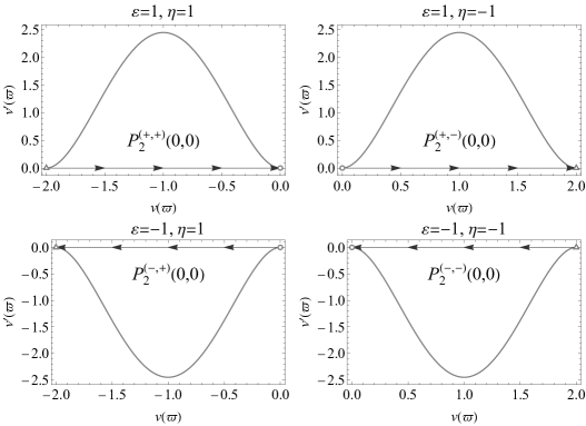
Figure 1: One-dimensional flow of the dynamical system (73) for $\varepsilon=\pm 1,\eta=\pm 1$. The points of interest $P_{2}^{(\pm,\pm)}$ are represented by open circles. Note that the center manifolds of the points $P_{2}^{(+,+)}$ and $P_{2}^{(-,-)}$ are stable, whereas the center manifolds of the points $P_{2}^{(+,-)}$ and $P_{2}^{(-,+)}$ are unstable.

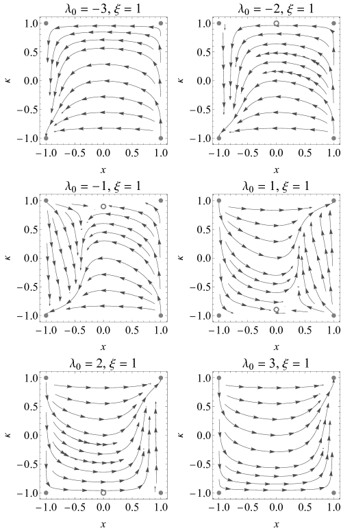
Figure 2: Phase-space portraits for the dynamical system (63), (64), for the value $\xi=1$ and various values of the free parameter $\lambda_{0}$. Closed circles denote the equilibrium points $P_{2}^{\left(\pm 1,\pm 1\right)}$ and open circles denote the equilibrium point $P_{1}(\kappa^{\star})$. For $\lambda_{0}<0$, point $P_{2}^{\left(-,-\right)}$ is the stable, late-time attractor, while for $\lambda_{0}>0$, point $P_{2}^{\left(+,+\right)}$ is the stable late-time solution of the system, and $P_{1}(\kappa^{\star})$ is a saddle.

The linearized matrix for the vector field (63)-(64) is

$$J=\left[\begin{array}[]{cc}J_{11}&J_{12}\\ J_{21}&J_{22}\\ \end{array}\right],$$ (67)

where

$$\!\!\!\!\!\!J_{11}=-3\sqrt{1-\kappa^{2}}+9\sqrt{1-\kappa^{2}}x^{2}$$

$$\ \ \ \ \ +\sqrt{6}x\left[2\kappa\left(\sqrt{\xi-\kappa^{2}\xi}-1\right)-\lambda_{0}\right]$$

$$\!\!\!\!\!\!J_{12}=-\frac{\left(x^{2}-1\right)\left\{\sqrt{6}\left[\left(2\kappa^{2}-1\right)\sqrt{\xi}+\sqrt{1-\kappa^{2}}\right]+3\kappa x\right\}}{\sqrt{1-\kappa^{2}}}$$

$$\!\!\!\!\!\!J_{21}=\sqrt{6}\left(1-\kappa^{2}\right)^{3/2}\sqrt{\xi}$$

$$\!\!\!\!\!\!J_{22}=-3\sqrt{6}\kappa x\sqrt{\xi-\kappa^{2}\xi}.$$ (68)

The Hartman-Grobman theorem or Center Manifold theorem relies on the fact that a system evolving in time as $u(t)\in\mathbb{R}^{n}$ must satisfy the differential equation $du/dt=f(u)$ for some smooth map $f:\mathbb{R}^{n}\to\mathbb{R}^{n}$ normally ; Strogatz . This is clearly not the case for the vector field (63)-(64) at $\kappa=\pm 1$, since $J$ is not continuous at $\kappa=\pm 1$ due to the fact that $J_{12}$ is not bounded at $\kappa=\pm 1$. Therefore, in order to conclude on the stability of $P_{2}^{\left(\varepsilon,\eta\right)}$ we need to perform a numerical elaboration. Introducing the variables

$$u=x-\varepsilon,\ \ \ v=\kappa-\eta,$$ (69)

we result to the dynamical system

$$\frac{du}{d\omega}= -\sqrt{\frac{3}{2}}\lambda_{0}u(u+2\varepsilon)$$

$$+3u\left(u^{2}+3u\varepsilon+2\right)\sqrt{-v(2\eta+v)}$$

$$+\sqrt{6}u(u+2\varepsilon)(\eta+v)\left[\sqrt{-\xi v(2\eta+v)}-1\right],$$ (70)

$$\frac{dv}{d\omega}= \frac{\sqrt{6}(u+\varepsilon)[-\xi v(2\eta+v)]^{3/2}}{\xi},$$ (71)

where we assume the $v$-range: $0\leq v\leq 2$ for $\eta=-1$, or $-2\leq v\leq 0$ for $\eta=+1$, as the physical ones. Although the corresponding linearization matrix is not bounded and is not continuous at $(u,v)=(0,0)$, we can obtain partial information about the stability at the origin by studying the invariant set $u=0$. The dynamics at the invariant set $u=0$ is given by

$$\frac{dv}{d\omega}=\frac{\sqrt{6}\varepsilon[-\xi v(2\eta+v)]^{3/2}}{\xi}.$$ (72)

By assuming $\xi>0$, and re-scaling time by $\frac{d}{d\varpi}=\sqrt{-v(2\eta+v)/\xi}\frac{d}{d\omega}$, we obtain

$$\frac{dv}{d\varpi}=\sqrt{6}\varepsilon v^{2}(2\eta+v)^{2},$$ (73)

where $0\leq v\leq 2$ for $\eta=-1$, or $-2\leq v\leq 0$ for $\eta=+1$, is the physical domain for $v$. In a one-dimensional phase space, $\frac{dv}{d\varpi}>0$ implies that the arrow is directed to the right, and $\frac{dv}{d\varpi}<0$ implies that the arrow is directed to the left Strogatz . Hence, from the analysis of the corresponding one-dimensional flow it follows that the center manifolds of the points $P^{(+,+)}$ and $P^{(-,-)}$ are stable, whereas the center manifolds of the points $P^{(+,-)}$ and $P^{(-,+)}$ are unstable. These results are illustrated in Fig. 1.

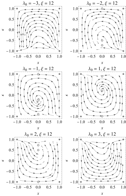
Figure 3: Phase-space portraits for the dynamical system (63), (64), for the value $\xi=12$ and various values of the free parameter $\lambda_{0}$. Closed circles denote the equilibrium points $P_{2}^{\left(\pm 1,\pm 1\right)}$ and open circles denote the equilibrium points of type $P_{1}(\kappa^{\star})$. For $\lambda_{0}<0$, point $P_{2}^{\left(-,-\right)}$ is the stable, late-time attractor, while for $\lambda_{0}>0$, point $P_{2}^{\left(+,+\right)}$ is the stable late-time solution of the system. One of the equilibrium points of type $P_{1}(\kappa^{\star})$ is stable (open circle in the middle of some graphs).

We continue by presenting the phase-space diagram for the dynamical system (63), (64) for various values of the free parameters $\xi~{}$and $\lambda_{0}$ in Figs. 2 and 3. As we observe in both figures for $\lambda_{0}>0$, point $P_{2}^{\left(+,+\right)}$ is the attractor, while for $\lambda_{0}<0$, point $P_{2}^{\left(-,-\right)}$ is the stable late-time solution of the system. For $\xi=1$, there is an equilibrium point $P_{1}(\kappa^{\star})$, which is saddle (see Fig. 2). Furthermore, for $\xi=12$, there are three equilibrium points of type $P_{1}(\kappa^{\star})$, and one of them can be stable (open circle in the middle of some graphs in Fig. 3).

Lastly, let us examine the special case where $\lambda=-2$. In this case for the additional curve of critical points $P_{3}^{+}$ we find that $w_{eff}\left(P_{3}^{+}\right)=-1+2x^{2}+4\sqrt{\frac{2\xi}{3}}x$. These points describe a de Sitter solution for $x\in\left\{0,-2\sqrt{\frac{2}{3}}\sqrt{\xi}\right\}$. Hence, the points of $P_{3}^{+}$ describe matter-dominated solutions when $x^{\pm}=-\frac{2\sqrt{\xi}\pm\sqrt{3+4\xi}}{\sqrt{6}}$. Moreover, as far as $\xi$ is concerned, for $x^{+}$ it follows $0<\xi<\frac{3}{32}$, while for $x^{-}$ we obtain $0<\xi$. Similarly, for the additional curve of points $P_{3}^{-}$ we find that $w_{eff}\left(P_{3}^{-}\right)=-1+2x^{2}-4\sqrt{\frac{2\xi}{3}}x$. These points describe de Sitter solutions for $x\in\left\{0,2\sqrt{\frac{2}{3}}\sqrt{\xi}\right\}$. $P_{3}^{-}$ describe matter-dominated universes when $x^{\pm}=\frac{2\sqrt{\xi}+\sqrt{4\xi+3}}{\sqrt{6}}$, and for $x^{+}$ it follows $0<\xi<\frac{3}{32}$, while for $x^{-}$ we acquire $0<\xi$.

IV.4 Unified dark sectors

We have now all the information to proceed to a unified description of the dark sectors. In particular, as we saw, the scenario of the scalar-torsion theory at hand possesses critical points in which the total, effective equation-of-state parameter of the universe behaves as dust matter and critical points in which it behaves as dark energy. Thus, with the single sector, we can describe both the matter and late-time acceleration epochs.

In Fig. 4 we depict the evolution of the effective equation-of-state parameter $w_{eff}$ for various choices of $\lambda$ and $\xi$. As we can see, the universe at intermediate times remains around the scaling solution in which $w_{eff}$ is close to zero, and hence this era corresponds to the dust matter-dominated phase. As time passes the universe enters into an accelerated phase in which $w_{eff}$ becomes smaller than $-1/3$, and at present time it becomes equal to $-0.7$ as required by observations. Finally, at asymptotically late times, the Universe will result in a de Sitter phase. Hence, using models of scalar-torsion theory we succeeded in describing the matter and late-time accelerated eras with a single sector, which was the goal of the present work.

Figure 4: Evolution of effective, total equation-of-state parameter $w_{eff}$ of the cosmological fluid in scalar-torsion theory, for $\lambda=2$ and $\xi=0.08$ (solid line), $\ \xi=0.09$ (dotted line) and $\xi=0.1$ (dashed line). We have imposed $w_{eff}\approx-0.7$ at present time $a=a_{0}=1$ as required by observations.

V Conclusions

We presented a unified description of the matter and dark energy epochs, using not a peculiar, exotic fluid, but a class of scalar-torsion theories. In particular, we started from the subclass of such theories in which a scalar field is non-minimally coupled with the torsion scalar and we provided a Hamiltonian description, focusing on the conservation laws. Then, by applying Noether’s theorem and by requiring the field equations to admit linear-in- momentum conservation laws we extracted two classes of potentials for the scalar field.

For the two scalar potentials we extracted analytic solutions and we performed a detailed dynamical analysis to extract the critical points and their properties and thus the global feature of the Universe evolution independently of the initial conditions. As we saw, the system possesses critical points that correspond to scaling solutions in which the effective, total equation-of-state parameter is close to zero, and points in which it is equal to the cosmological constant value $-1$. Therefore, during its evolution, the Universe remains for sufficiently long times around the scaling solutions, i.e. in the epoch corresponding to dust-matter domination, while at later times $w_{eff}$ decreases and becomes smaller than $-1/3$, which marks the onset of the acceleration. Then, at present it is equal to $-0.7$, as required by observations, while at asymptotically late times the Universe results in the de Sitter phase. In summary, using scalar-torsion theory we succeeded in describing the matter and late-time accelerated eras with a single sector.

We close this section by referring to the additional important advantage of the scenario at hand, which is related to the stability at the perturbation level. As we mentioned in the Introduction, although a unification of the dark sectors can be obtained through Chaplygin gas-based models as well as in Horndeski-based constructions, in both cases perturbative instabilities, and pathologies related to the sound-speed square, may appear at the perturbation level. On the contrary, the scalar-tensor theories applied in this work is known to be free from instabilities and pathologies at the perturbative level Hohmann:2017qje ; DAgostino:2018ngy ; Gonzalez-Espinoza:2021mwr ; Bahamonde:2021dqn ; Toporensky:2021poc . This feature acts in favor of the robustness of the present scenarios. We should further confront the perturbations of the scenario at hand with growth data too, however, this important investigation lies beyond the scope of the present work and it is left for a future project.

- (1) E. J. Copeland, M. Sami and S. Tsujikawa, Int. J. Mod. Phys. D 15, 1753 (2006) [hep-th/0603057].
- (2) Y. F. Cai, E. N. Saridakis, M. R. Setare and J. Q. Xia, Phys. Rept. 493, 1 (2010) [arXiv:0909.2776 [hep-th]].
- (3) E. N. Saridakis et al. [CANTATA], [arXiv:2105.12582 [gr-qc]].
- (4) S. Capozziello and M. De Laurentis, Phys. Rept. 509, 167 (2011) [arXiv:1108.6266 [gr-qc]].
- (5) S. Nojiri and S. D. Odintsov, Phys. Rept. 505, 59 (2011) [arXiv:1011.0544 [gr-qc]].
- (6) A. R. Liddle and D. H. Lyth, Phys. Rept. 231, 1-105 (1993) [arXiv:astro-ph/9303019 [astro-ph]].
- (7) N. Aghanim et al. [Planck], Astron. Astrophys. 641, A6 (2020) [erratum: Astron. Astrophys. 652, C4 (2021)] [arXiv:1807.06209 [astro-ph.CO]].
- (8) E. Abdalla, G. F. Abellán, A. Aboubrahim, A. Agnello, O. Akarsu, Y. Akrami, G. Alestas, D. Aloni, L. Amendola and L. A. Anchordoqui, et al. [arXiv:2203.06142 [astro-ph.CO]].
- (9) S. Nojiri and S. D. Odintsov, Phys. Rev. D 74, 086005 (2006) [arXiv:hep-th/0608008 [hep-th]].
- (10) B. Famaey and S. McGaugh, Living Rev. Rel. 15, 10 (2012) [arXiv:1112.3960 [astro-ph.CO]].
- (11) L. Sebastiani, S. Vagnozzi and R. Myrzakulov, Adv. High Energy Phys. 2017, 3156915 (2017) [arXiv:1612.08661 [gr-qc]].
- (12) A. Addazi, J. Alvarez-Muniz, R. A. Batista, G. Amelino-Camelia, V. Antonelli, M. Arzano, M. Asorey, J. L. Atteia, S. Bahamonde and F. Bajardi, et al. [arXiv:2111.05659 [hep-ph]].
- (13) A. De Felice and S. Tsujikawa, Living Rev. Rel. 13, 3 (2010) [arXiv:1002.4928 [gr-qc]].
- (14) S. ’i. Nojiri and S. D. Odintsov, Phys. Lett. B 631, 1 (2005) [hep-th/0508049].
- (15) A. De Felice and S. Tsujikawa, Phys. Lett. B 675, 1 (2009) [arXiv:0810.5712 [hep-th]].
- (16) D. Lovelock, J. Math. Phys. 12, 498 (1971).
- (17) N. Deruelle and L. Farina-Busto, Phys. Rev. D 41, 3696 (1990).
- (18) G. W. Horndeski, Int. J. Theor. Phys. 10, 363-384 (1974)
- (19) A. De Felice and S. Tsujikawa, Phys. Rev. D 84, 124029 (2011) [arXiv:1008.4236 [hep-th]].
- (20) C. Deffayet, X. Gao, D. A. Steer and G. Zahariade, Phys. Rev. D 84, 064039 (2011) [arXiv:1103.3260 [hep-th]].
- (21) R. Aldrovandi and J. G. Pereira, Teleparallel Gravity: An Introduction, Springer, Dordrecht (2013).
- (22) J. W. Maluf, Annalen Phys. 525, 339 (2013).
- (23) Y. F. Cai, S. Capozziello, M. De Laurentis and E. N. Saridakis, Rept. Prog. Phys. 79, no. 10, 106901 (2016) [arXiv:1511.07586 [gr-qc]].
- (24) R. Ferraro and F. Fiorini, Phys. Rev. D 75, 084031 (2007) [gr-qc/0610067].
- (25) E. V. Linder, Phys. Rev. D 81, 127301 (2010) Erratum: [Phys. Rev. D 82, 109902 (2010)] [arXiv:1005.3039 [astro-ph.CO]].
- (26) G. Kofinas and E. N. Saridakis, Phys. Rev. D 90, 084044 (2014) [arXiv:1404.2249 [gr-qc]].
- (27) S. Bahamonde, C. G. Böhmer and M. Wright, Phys. Rev. D 92, no.10, 104042 (2015) [arXiv:1508.05120 [gr-qc]].
- (28) C. Q. Geng, C. C. Lee, E. N. Saridakis and Y. P. Wu, Phys. Lett. B 704, 384-387 (2011) [arXiv:1109.1092 [hep-th]].
- (29) C. Q. Geng, C. C. Lee and E. N. Saridakis, JCAP 01, 002 (2012) [arXiv:1110.0913 [astro-ph.CO]].
- (30) M. Gonzalez-Espinoza and G. Otalora, Eur. Phys. J. C 81, no.5, 480 (2021) [arXiv:2011.08377 [gr-qc]].
- (31) A. Paliathanasis, [arXiv:2107.05880 [gr-qc]].
- (32) M. Gonzalez-Espinoza, R. Herrera, G. Otalora and J. Saavedra, Eur. Phys. J. C 81, no.8, 731 (2021) [arXiv:2106.06145 [gr-qc]].
- (33) A. V. Toporensky and P. V. Tretyakov, [arXiv:2110.12332 [gr-qc]].
- (34) G. Kofinas, E. Papantonopoulos and E. N. Saridakis, Phys. Rev. D 91, no.10, 104034 (2015) [arXiv:1501.00365 [gr-qc]].
- (35) C. Q. Geng, C. C. Lee and H. H. Tseng, JCAP 11, 013 (2012) [arXiv:1207.0579 [gr-qc]].
- (36) M. A. Skugoreva, E. N. Saridakis and A. V. Toporensky, Phys. Rev. D 91, 044023 (2015) [arXiv:1412.1502 [gr-qc]].
- (37) L. Jarv and A. Toporensky, Phys. Rev. D 93, no.2, 024051 (2016) [arXiv:1511.03933 [gr-qc]].
- (38) M. A. Skugoreva and A. V. Toporensky, Eur. Phys. J. C 76, no.6, 340 (2016) [arXiv:1605.01989 [gr-qc]].
- (39) M. Hohmann, L. Järv and U. Ualikhanova, Phys. Rev. D 97, no.10, 104011 (2018) [arXiv:1801.05786 [gr-qc]].
- (40) M. Hohmann, Phys. Rev. D 98, no.6, 064002 (2018) [arXiv:1801.06528 [gr-qc]].
- (41) M. Hohmann, Phys. Rev. D 98, no.6, 064004 (2018) [arXiv:1801.06531 [gr-qc]].
- (42) M. Hohmann and C. Pfeifer, Phys. Rev. D 98, no.6, 064003 (2018) [arXiv:1801.06536 [gr-qc]].
- (43) E. D. Emtsova and M. Hohmann, Phys. Rev. D 101, no.2, 024017 (2020) [arXiv:1909.09355 [gr-qc]].
- (44) S. Bahamonde, K. F. Dialektopoulos and J. Levi Said, Phys. Rev. D 100, no.6, 064018 (2019) [arXiv:1904.10791 [gr-qc]].
- (45) S. Bahamonde, K. F. Dialektopoulos, M. Hohmann and J. Levi Said, Class. Quant. Grav. 38, no.2, 025006 (2020) [arXiv:2003.11554 [gr-qc]].
- (46) S. Bahamonde, M. Caruana, K. F. Dialektopoulos, V. Gakis, M. Hohmann, J. Levi Said, E. N. Saridakis and J. Sultana, Phys. Rev. D 104, no.8, 084082 (2021) [arXiv:2105.13243 [gr-qc]].
- (47) R. C. Bernardo, J. L. Said, M. Caruana and S. Appleby, JCAP 10, 078 (2021) [arXiv:2107.08762 [gr-qc]].
- (48) N. Bilic, G. B. Tupper and R. D. Viollier, Phys. Lett. B 535, 17-21 (2002) [arXiv:astro-ph/0111325 [astro-ph]].
- (49) M. C. Bento, O. Bertolami and A. A. Sen, Phys. Rev. D 66, 043507 (2002) [arXiv:gr-qc/0202064 [gr-qc]].
- (50) A. Dev, D. Jain and J. S. Alcaniz, Phys. Rev. D 67, 023515 (2003) [arXiv:astro-ph/0209379 [astro-ph]].
- (51) G. Koutsoumbas, K. Ntrekis, E. Papantonopoulos and E. N. Saridakis, JCAP 02, 003 (2018) [arXiv:1704.08640 [gr-qc]].
- (52) M. d. C. Bento, O. Bertolami and A. A. Sen, Phys. Rev. D 67, 063003 (2003) [astro-ph/0210468].
- (53) M. C. Bento, O. Bertolami, M. J. Reboucas and P. T. Silva, Phys. Rev. D 73, 043504 (2006) [gr-qc/0512158].
- (54) H. Sandvik, M. Tegmark, M. Zaldarriaga and I. Waga, Phys. Rev. D 69, 123524 (2004) [astro-ph/0212114].
- (55) M. U. Farooq, M. Jamil and M. A. Rashid, Int. J. Theor. Phys. 49, 2334 (2010) [arXiv:1003.3399 [gr-qc]].
- (56) V. Gorini, A. Y. Kamenshchik, U. Moschella, O. F. Piattella and A. A. Starobinsky, JCAP 0802, 016 (2008) [arXiv:0711.4242 [astro-ph]].
- (57) U. Debnath, A. Banerjee and S. Chakraborty, Class. Quant. Grav. 21, 5609 (2004) [gr-qc/0411015].
- (58) M. Bouhmadi-Lopez and P. Vargas Moniz, Phys. Rev. D 71, 063521 (2005) [gr-qc/0404111].
- (59) M. R. Setare, Phys. Lett. B 654, 1 (2007) [arXiv:0708.0118 [hep-th]].
- (60) E. Babichev, V. Mukhanov and A. Vikman, JHEP 02, 101 (2008) [arXiv:0708.0561 [hep-th]].
- (61) C. Deffayet, O. Pujolas, I. Sawicki and A. Vikman, JCAP 10, 026 (2010) [arXiv:1008.0048 [hep-th]].
- (62) D. A. Easson, I. Sawicki and A. Vikman, JCAP 07, 014 (2013) [arXiv:1304.3903 [hep-th]].
- (63) K. Rosquist and C. Uggla, J. Math. Phys. 32, 3412 (1991).
- (64) S. Cotsakis, P. Leach and H. Pantazi, Grav. Cosmol. 4, 314-325 (1998) [arXiv:gr-qc/0011017 [gr-qc]].
- (65) B. Vakili, Phys. Lett. B 664, 16-20 (2008) [arXiv:0804.3449 [gr-qc]].
- (66) S. Capozziello, E. Piedipalumbo, C. Rubano and P. Scudellaro, Phys. Rev. D 80, 104030 (2009) [arXiv:0908.2362 [astro-ph.CO]].
- (67) Y. Zhang, Y. g. Gong and Z. H. Zhu, Phys. Lett. B 688, 13-20 (2010) [arXiv:0912.0067 [hep-ph]].
- (68) H. Mohseni Sadjadi, Phys. Lett. B 718, 270-275 (2012) [arXiv:1210.0937 [gr-qc]].
- (69) B. Vakili and F. Khazaie, Class. Quant. Grav. 29, 035015 (2012) [arXiv:1109.3352 [gr-qc]].
- (70) K. Atazadeh and F. Darabi, Eur. Phys. J. C 72, 2016 (2012) [arXiv:1112.2824 [physics.gen-ph]].
- (71) H. Dong, J. Wang and X. Meng, Eur. Phys. J. C 73, no.8, 2543 (2013) [arXiv:1304.6587 [gr-qc]].
- (72) T. Christodoulakis, N. Dimakis, P. A. Terzis and G. Doulis, Phys. Rev. D 90, no.2, 024052 (2014) [arXiv:1405.0363 [gr-qc]].
- (73) P. A. Terzis, N. Dimakis and T. Christodoulakis, Phys. Rev. D 90, no.12, 123543 (2014) [arXiv:1410.0802 [gr-qc]].
- (74) N. Dimakis, T. Christodoulakis and P. A. Terzis, J. Geom. Phys. 77, 97-112 (2014) [arXiv:1311.4358 [gr-qc]].
- (75) N. Dimakis, A. Giacomini, S. Jamal, G. Leon and A. Paliathanasis, Phys. Rev. D 95, no.6, 064031 (2017) [arXiv:1702.01603 [gr-qc]].
- (76) A. Paliathanasis, M. Tsamparlis and S. Basilakos, Phys. Rev. D 90, no.10, 103524 (2014) [arXiv:1410.4930 [gr-qc]].
- (77) G. Papagiannopoulos, J. D. Barrow, S. Basilakos, A. Giacomini and A. Paliathanasis, Phys. Rev. D 95, no.2, 024021 (2017) [arXiv:1611.00667 [gr-qc]].
- (78) A. Paliathanasis, M. Tsamparlis and S. Basilakos, Phys. Rev. D 84, 123514 (2011) [arXiv:1111.4547 [astro-ph.CO]].
- (79) A. Paliathanasis, Class. Quant. Grav. 33, no.7, 075012 (2016) [arXiv:1512.03239 [gr-qc]].
- (80) S. Basilakos, S. Capozziello, M. De Laurentis, A. Paliathanasis and M. Tsamparlis, Phys. Rev. D 88, 103526 (2013) [arXiv:1311.2173 [gr-qc]].
- (81) A. Paliathanasis, S. Basilakos, E. N. Saridakis, S. Capozziello, K. Atazadeh, F. Darabi and M. Tsamparlis, Phys. Rev. D 89, 104042 (2014) [arXiv:1402.5935 [gr-qc]].
- (82) L. Karpathopoulos, S. Basilakos, G. Leon, A. Paliathanasis and M. Tsamparlis, Gen. Rel. Grav. 50, no.7, 79 (2018) [arXiv:1709.02197 [gr-qc]].
- (83) S. Capozziello, M. De Laurentis and K. F. Dialektopoulos, Eur. Phys. J. C 76, no.11, 629 (2016) [arXiv:1609.09289 [gr-qc]].
- (84) S. Bahamonde and S. Capozziello, Eur. Phys. J. C 77, no.2, 107 (2017) [arXiv:1612.01299 [gr-qc]].
- (85) S. Basilakos, M. Tsamparlis and A. Paliathanasis, Phys. Rev. D 83, 103512 (2011) [arXiv:1104.2980 [astro-ph.CO]].
- (86) M. Tsamparlis and A. Paliathanasis, Symmetry 10, no.7, 233 (2018) [arXiv:1806.05888 [gr-qc]].
- (87) E. J. Copeland, A. R. Liddle and D. Wands, Phys. Rev. D 57, 4686-4690 (1998) [arXiv:gr-qc/9711068 [gr-qc]].
- (88) R. Lazkoz, G. Leon and I. Quiros, Phys. Lett. B 649, 103-110 (2007) [arXiv:astro-ph/0701353 [astro-ph]].
- (89) C. R. Fadragas and G. Leon, Class. Quant. Grav. 31, no.19, 195011 (2014) [arXiv:1405.2465 [gr-qc]].
- (90) L. Amendola, D. Polarski and S. Tsujikawa, Phys. Rev. Lett. 98, 131302 (2007) [arXiv:astro-ph/0603703 [astro-ph]].
- (91) R. Lazkoz and G. Leon, Phys. Lett. B 638, 303-309 (2006) [arXiv:astro-ph/0602590 [astro-ph]].
- (92) G. Leon, Class. Quant. Grav. 26, 035008 (2009) [arXiv:0812.1013 [gr-qc]].
- (93) G. Leon and E. N. Saridakis, JCAP 03, 025 (2013) [arXiv:1211.3088 [astro-ph.CO]].
- (94) S. Basilakos, G. Leon, G. Papagiannopoulos and E. N. Saridakis, Phys. Rev. D 100, no.4, 043524 (2019) [arXiv:1904.01563 [gr-qc]].
- (95) C. R. Fadragas, G. Leon and E. N. Saridakis, Class. Quant. Grav. 31, 075018 (2014) [arXiv:1308.1658 [gr-qc]].
- (96) A. Paliathanasis and G. Leon, Class. Quant. Grav. 38, no.7, 075013 (2021) [arXiv:2009.12874 [gr-qc]].
- (97) G. Papagiannopoulos, S. Basilakos and E. N. Saridakis, [arXiv:2202.10871 [gr-qc]].
- (98) B. Aulbach, Continuous and discrete dynamics near manifolds of equilibria, Lecture Notes in Mathematics, No 1058, Springer-Verlag (1981).
- (99) S. Strogatz, Nonlinear dynamics and chaos : with applications to physics, biology, chemistry and engineering, CRC Press, Boca Raton, Florida (2018).
- (100) M. Hohmann and A. Schärer, Phys. Rev. D 96, no.10, 104026 (2017) [arXiv:1708.07851 [gr-qc]].
- (101) R. D’Agostino and O. Luongo, Phys. Rev. D 98, no.12, 124013 (2018) [arXiv:1807.10167 [gr-qc]].
- (102) M. Gonzalez-Espinoza, G. Otalora and J. Saavedra, JCAP 10, 007 (2021) [arXiv:2101.09123 [gr-qc]].