Time-inhomogeneous diffusion geometry and topology

Abstract

Diffusion condensation is a dynamic process that yields a sequence of multiscale data representations that aim to encode meaningful abstractions. It has proven effective for manifold learning, denoising, clustering, and visualization of high-dimensional data. Diffusion condensation is constructed as a time-inhomogeneous process where each step first computes and then applies a diffusion operator to the data. We theoretically analyze the convergence and evolution of this process from geometric, spectral, and topological perspectives. From a geometric perspective, we obtain convergence bounds based on the smallest transition probability and the radius of the data, whereas from a spectral perspective, our bounds are based on the eigenspectrum of the diffusion kernel. Our spectral results are of particular interest since most of the literature on data diffusion is focused on homogeneous processes. From a topological perspective, we show diffusion condensation generalizes centroid-based hierarchical clustering. We use this perspective to obtain a bound based on the number of data points, independent of their location. To understand the evolution of the data geometry beyond convergence, we use topological data analysis. We show that the condensation process itself defines an intrinsic condensation homology. We use this intrinsic topology as well as the ambient persistent homology of the condensation process to study how the data changes over diffusion time. We demonstrate both types of topological information in well-understood toy examples. Our work gives theoretical insights into the convergence of diffusion condensation, and shows that it provides a link between topological and geometric data analysis.

57M50, 57R40, 62R40, 37B25, 68xxx

1 Introduction

Graph representations of high-dimensional data have proven useful in many applications such as visualization, clustering, and denoising. Typically, a set of data points is described by a graph using a pairwise affinity measure, stored in an affinity matrix. With this matrix, one can define the random walk operator or the graph Laplacian, and use numerous tools from graph theory to characterize the input data. Diffusion operators are closely related to random walks on a graph, as they describe how heat (or gas) propagates across the vertices. Using powers of this operator yields a time-homogeneous Markov process that has been extensively studied. Most notably, Coifman et al. [11] proved that, under specific conditions, this operator converges to the heat kernel on an underlying continuous manifold. Manifold learning methods like diffusion maps [11] define an embedding via the eigendecomposition of the diffusion operator. Other methods, such as PHATE [31], embed a diffusion-based distance by multidimensional scaling. Various clustering algorithms rely on the eigendecomposition of this operator (or the resulting Laplacian) [28, 39]. However, this homogeneous process requires a bandwidth in order to fix and determine the scale of the captured data manifold. If we are interested in considering multiple scales of the data [3, 25], or if the data is sampled from a time-varying manifold [29], we need a time-inhomogenous process.

In this paper, we focus on the time-inhomogeneous diffusion process for a given initial set of data points. This process is known as Diffusion Condensation [3] and yields a representation of the data by a sequence of datasets, each at a different granularity. This sequence is obtained by iteratively applying a diffusion operator. It has proven effective for tasks such as denoising, clustering, and manifold learning [3, 25, 29, 35, 36]. In this work, we study theoretical questions of diffusion condensation. Thus, we define conditions on the diffusion operators such that the process converges to a single point. The convergence to a point is a valuable characteristic, as it is a necessary condition for any process that sweeps a complete range of granularities of the data. We present this analysis from a geometric and a spectral perspective, addressing different families of operators. We also study how the intrinsic shape of the condensed datasets evolves through condensation time using tools from topological data analysis. In particular, we define an intrinsic filtration based on the condensation process, resulting in the notions of persistent and condensation homology, for studying individual condensation steps or for summarizing the entire process, respectively. Making use of a topological perspective, we also prove the relation between diffusion condensation and types of hierarchical clustering algorithms.

The paper is organized as follows. In Section 2, we present an overview of diffusion condensation. In Section 3, we develop a geometric analysis of the process, most importantly we prove its convergence to a point. In Section 4, we study the convergence of the process from a spectral perspective. In Section 5, we present a topological analysis of the process and relate diffusion condensation to existing hierarchical clustering algorithms.

2 Diffusion condensation

In order to establish the setup and scope for our work, we first formalize here the diffusion condensation framework, and provide a unifying view of design choices and algorithms used to empirically evaluate its efficacy in previous and related work.

2.1 Notations and setup

Let $\mathsf{X}=\{x(j):j=1,\ldots,N\}\subset\mathds{R}^{d}$ be an input dataset of $N$ data points in $d$ dimensions. Given a symmetric nonnegative affinity kernel $k:\mathds{R}^{d}\times\mathds{R}^{d}\rightarrow\mathds{R}$, with $0\leq k(x,y)=k(y,x)\leq 1$, $x,y\in\mathds{R}^{d}$, we define an $N\times N$ kernel matrix $\mathbf{K}$ with entries $\mathbf{K}(i,j):=k(x(i),x(j))$, which can be regarded as a weighted adjacency matrix of a graph capturing the intrinsic geometry of the data. Furthermore, the kernel and resulting graph are often considered as providing a notion of locality in the data, which can be tuned by a kernel bandwidth parameter $\epsilon$. We defer discussion of specific $k$ dependent on $\epsilon$ to Section 2.5, but mention that it can be regarded as a proxy for the size or (local) radius of the neighborhoods defined by the kernel. The diffusion framework for manifold learning [11, 31] uses this construction to define a Markov process over the intrinsic structure of the data by normalizing the kernel matrix with a diagonal degree matrix $\mathbf{D}:=\mathrm{diag}(d(1),d(2),\ldots,d(N))$ where $d(i):=\sum_{j}\mathbf{K}(i,j)$, resulting in a row stochastic Markov matrix $\mathbf{P}:=\mathbf{D}^{-1}\mathbf{K}$, known as the (discrete) diffusion operator. Traditionally, time-homogeneous diffusion processes leverage powers $\mathbf{P}^{\tau}$ of this diffusion operator, for diffusion times $\tau\in\mathds{N}$, to capture underlying data-manifold structure in $\mathsf{X}$ and to organize the data along this structure [11, 31].

Here, on the other hand, we follow the diffusion condensation approach [3] and use a time-inhomogeneous process, where the diffusion operator (and underlying finite dataset) vary over time. We consider a sequence of datasets $\mathsf{X}_{t}=\{x_{t}(j):j=1,\ldots,N\}$, ordered along diffusion condensation time $t\in\mathds{N}$, with corresponding diffusion operators $\mathbf{P}_{t}$, each constructed over the corresponding $\mathsf{X}_{t}$. With a slight abuse of notation we often refer to $\mathsf{X}_{t}$ as a set or as an $N\times d$ matrix, where $x_{t}(j)$ is the j-th row or equivalently the j-th element of the set. At time $t=0$ we consider the input dataset, with its (traditional) diffusion operator, while for each $t>0$ we take $\mathsf{X}_{t}:=\mathbf{P}^{\tau}_{t-1}\mathsf{X}_{t-1}$, with the usual matrix multiplication. Then, instead of powers of a single diffusion operator, the $t$-step condensation process is defined via $\mathbf{P}^{(t-1)}:=\mathbf{P}^{\tau}_{t-1}\dotsm\mathbf{P}^{\tau}_{0}$, and thus we can also directly write $\mathsf{X}_{t}=\mathbf{P}^{(t-1)}\mathsf{X}_{0}$. Note that $\mathbf{P}^{(t-1)}$ is constructed from a collection of operators based on different datasets, and potentially different bandwidth parameters or kernels, therefore making the process time-inhomegenous. For simplicity, we keep the diffusion time $\tau$, but it could also depend on the condensation time $t$. Finally, we use the notation $\mathsf{X}^{(T)}:=\mathsf{X}_{0},\mathsf{X}_{1},\dots,\mathsf{X}_{T}$ for a sequence of datasets up to finite time $T$, and denote the diameter of the dataset at time $t$ as $\operatorname{diam}(\mathsf{X}_{t}):=\max_{x,y\in\mathsf{X}_{t}}\|x-y\|_{2}$.

2.2 Related work using diffusion condensation for data analysis and open questions

The diffusion condensation algorithm first proposed in Brugnone et al. [3] has been applied for data analysis in a number of areas. Moyle et al. [32] applied diffusion condensation to study neural connectomics between species and identify biologically meaningful substructures. Kuchroo et al. [25] applied diffusion condensation to embed and visualize single-cell proteomic data to explore the effect of COVID-19 on the immune system. Kuchroo et al. [24] applied diffusion condensation on single-nucleus RNA sequencing data from human retinas with age-related macular degeneration (AMD) and found a potential drug target by exploring the topological structure of the resulting diffusion condensation process. van Dijk et al. [36] applied one step of diffusion condensation ($T=1$) with high $\tau$ to single-cell RNA sequencing data to impute gene expression. They showed that high $\tau$ improves the quality of downstream tasks such as gene-gene relationships and visualization. These works demonstrate the empirical utility of diffusion condensation in a number of settings, specifically when multiscale clustering and visualization is needed and the data lies on a manifold.

The diffusion condensation process is a particular type of time-inhomogeneous diffusion process. General time-inhomogeneous diffusion processes over time-varying data were studied in [29], where it was proposed to use the singular value decomposition of the operator $\mathbf{P}^{(t)}$ to embed an arbitrary sequence of datasets $\mathsf{X}^{(T)}$ according to their space-time geometry. Additionally, if those datasets $\mathsf{X}^{(T)}$ were sampled from a manifold $(\mathcal{M},g(t))$ with time-varying metric tensor $g(t)$, it was shown in [29] that as $N,T\rightarrow\infty$, the operator $\mathbf{P}^{(t)}$ converges to the heat kernel of $(\mathcal{M},g(t))$. We also note a resemblance to the mean shift algorithm [17, 8], which relies on a kernel-based estimation of $\nabla\log p(x)$, where $p(x)$ is the unknown density from which the points are sampled. The processed dataset is recursively updated via $x_{t+1}(i)=x_{t}(i)+\epsilon\nabla\log p(x)$, which effectively moves all points toward a mode of the distribution, hence creating clusters.

Motivated by these empirical successes and inspired by the general theoretical results on time-inhomogeneous diffusion processes, we consider two open questions specific to the diffusion condensation process. Under what conditions does the diffusion condensation algorithm converge? How can the topology of the diffusion condensation process be understood?

2.3 Theoretical contributions

The main contribution of this paper is to address these open questions and establish the underpinnings of diffusion condensation. Our investigation is divided into three perspectives. First, we investigate the convergence properties of diffusion condensation under various parameter regimes from a geometric perspective in Section 3, i.e., arrangement of data points in spatial coordinates. This geometric perspective gives an intuitive sense of convergence for a large family of kernels with minimum tail bounds. Next, in Section 4, we investigate convergence from a spectral graph theory perspective and prove convergence in terms of the spectral properties of the kernel, viewing diffusion condensation as a non-stationary Markov process. A spectral perspective gives bounds in terms of the eigenvalues of the kernel, which can give better rates of convergence depending on considered data. Finally, in Section 5, we investigate the topological characteristics of diffusion condensation. Here we describe both the structure of the dataset at each condensation step individually via its persistent homology, as well as the topology of the condensation process itself, which we refer to as condensation homology. Additionally, we link the topology of the diffusion condensation process to hierarchical clustering and prove how it generalizes centroid linkage.

2.4 Algorithm

Algorithm 1 Diffusion Condensation

1:  Input: Dataset $\mathsf{X}_{0}$, initial kernel parameter $\epsilon_{0}$, diffusion time $\tau$, and merge radius $\zeta$

2:  Output: Condensed datasets $\mathsf{X}^{(T)}$

3:  for $t\in\{0,1,\dotsc,T-1\}$ do

4:     $\mathbf{K}_{t}\leftarrow\textup{kernel}(\mathsf{X}_{t},\epsilon_{t})$

5:     $\mathbf{P}_{t}\leftarrow\mathbf{D}^{-1}_{t}\mathbf{K}_{t}$

6:     $\mathsf{X}_{t+1}\leftarrow\mathbf{P}_{t}^{\tau}\mathsf{X}_{t}$

7:     $\epsilon_{t+1}\leftarrow\textup{update}(\epsilon_{t},\mathsf{X}_{t+1})$

8:     for $x_{t}(i),x_{t}(j)\in\mathsf{X}_{t}$ do

9:        $\textup{merge}(x_{t}(i),x_{t}(j))\text{ if }\|x_{t}(i)-x_{t}(j)\|_{2}<\zeta$

10:     end for

11:  end for

12:  $\mathsf{X}^{(T)}\leftarrow\{\mathsf{X}_{0},\mathsf{X}_{1},\ldots,\mathsf{X}_{T}\}$

The diffusion condensation algorithm summarizes input data with a series of representations, organized by condensation time, with earlier representations providing low level, microscopic details and later representations providing overall, macroscopic summarizations. Each time step of diffusion condensation can be broken up into five main steps.

1. Construct a kernel matrix $\mathbf{K}_{t}$ summarizing similarities between points.

2. Construct a Markov normalized diffusion operator $\mathbf{P}_{t}$.

3. Diffuse the data coordinates $\tau$ steps using $\mathbf{P}_{t}^{\tau}$.

4. Update the kernel bandwidth $\epsilon$ according to some update function.

5. (Optionally) merge points within distance $\zeta$.

Algorithm 1 shows pseudocode for this process. At each time step, the positions of points are updated based on the predefined kernel through $\tau$ steps of diffusion. Intuitively, this can be thought of as moving each point to a kernel-weighted average of its neighbors, The condensation process will behave differently depending on the choice of kernel, the kernel bandwidth, the diffusion time, and the merging threshold.

Fig. 1 depicts the differences between time-homogenous condensation, time inhomogenous condensation, and a mixture between the two. Greater values of $\tau$ encourage the process to condense along the manifold, in contrast with other hierarchical clustering algorithms that are not able to do so. Comparing only inhomogenous condensation $\mathbf{P}_{3i}$ (top) with a mixture of homogenous and inhomogenous condensation $\mathbf{P}^{3}_{i}$ (middle) we see that the mixture condenses the moon structures along the manifold rather than shattering them. Both of these are able to separate out the two clusters. In contrast, the fully time-homogenous condensation process $\mathbf{P}^{3i}$ (bottom) mixes eventually mixes the two moons. For the rest of the paper, we let $\tau=1$, but our results are valid for any $\tau\in\mathds{N}$. Only for the spectral part, we need to consider a slight nuance, which we discuss in Remark 4.11.

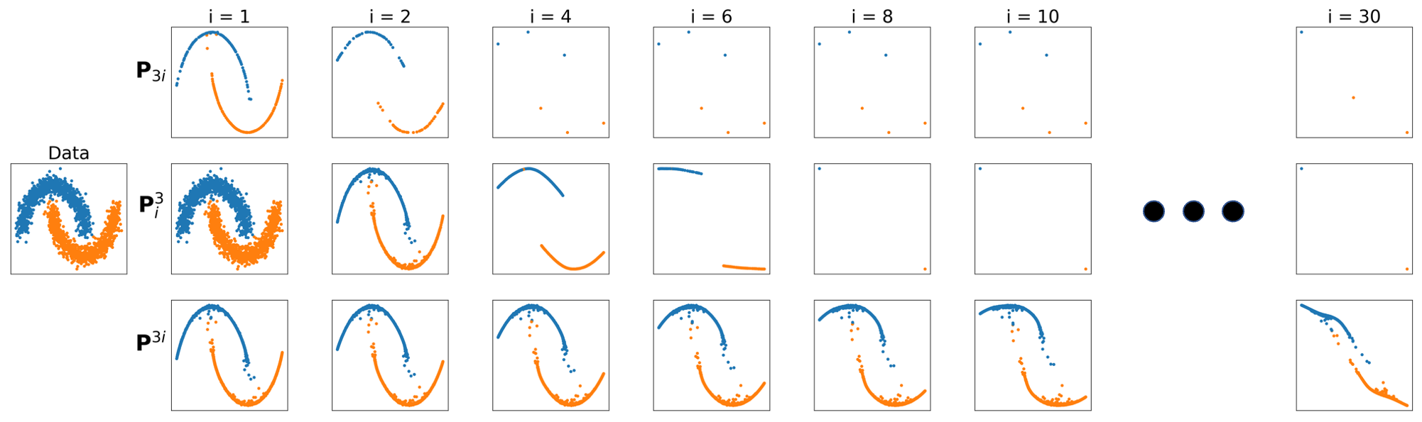
Figure 1: Shows the effects of powering the diffusion operator with a power $\tau$ before condensing on the moons dataset. Shows from top to bottom the time-inhomogenous process with $\tau=1$, with $\tau=3$, and the time-homogenous process with $T=1$ while varying $\tau$. For step $i$ this corresponds to comparing the applications of $\mathbf{P}_{3i}$, $\mathbf{P}^{3}_{i}$, and $\mathbf{P}^{3i}$ to the data. $\mathbf{P}_{3i}$ eventually merges, but has a semi-stable state of 6 points after shattering the moons. $\mathbf{P}^{3}_{i}$ correctly identifies the two clusters of the data efficiently by first condensing along the moons individually into points. Time-homogenous condensation $\mathbf{P}^{3t}$ mixes the two moons.

Remark 2.1.

The time-homogeneous equivalent of the condensation process would be to recursively apply the same diffusion operator $\mathbf{P}_{0}$ on the initial dataset $\mathsf{X}_{0}$. After $t$ iterations, the new dataset would simply be $\mathbf{P}_{0}^{t}\mathsf{X}_{0}$. This constrasts with the time-inhomegeneous version where we create a new diffusion operator at each iteration. Concequently, after $t$ iterations, the new dataset is $\mathbf{P}_{t-1}\dotsc\mathbf{P}_{1}\mathbf{P}_{0}\mathsf{X}_{0}$. By using a time-inhomogeneous process, we gain more control over the convergence behavior. Indeed, since we allow for modifications of the diffusion probabilities, we can define a schedule for the parameters that could either promote or slow down the convergence of the process. Here, for simplicity, we assumped $\tau=1$, but the same remark follows for any diffusion time $\tau\in\mathds{N}$.

2.5 Kernels for diffusion condensation

Here, we review specific kernel constructions used to study condensation properties in later sections. In Fig. 2, we present a few iterations of the condensation process, depending on the choice of kernel used to construct the diffusion matrix.

Definition 2.2 (Box Kernel).

The box kernel of bandwidth $\epsilon$ is

(1) $$k_{\epsilon}(x,y)=\begin{cases}1&\text{ if }\|x-y\|_{2}\leq\epsilon\\ 0&\text{ else}.\end{cases}$$

The box kernel is arguably the simplest and most interpretable kernel, leading to interesting data summarizations, including an instance of agglomerate clustering depending on the bandwidth as a function of time. However, first we note some simple cases of bandwidth settings. Consider a case where $k_{t}(x,y)=1$ for all $x,y\in\mathsf{X}_{0}$. This can be thought of as a box kernel with bandwidth greater than $\operatorname{diam}(\mathsf{X}_{0})$. Using this kernel, after a single step of diffusion condensation, all points converge to the mean data point, $\frac{1}{n}\sum_{i}x_{t}(i)$. This mean data point is a useful, if trivial, summarization of the data. Next, consider the opposite extreme, a box kernel with infinitely narrow bandwidth, $k_{t}(x,y)=\{1\text{ if }x=y\text{ else }0\}$. In this case, we have $\mathsf{X}_{t}=\mathsf{X}_{0}$ for all $t>0$, resulting in another trivial result, i.e., no data summarization over diffusion condensation time. Of more interest are bandwidths between these two extremes, providing hierarchical sets of summarizations. Next, we consider smoother kernels.

Definition 2.3.

The $\alpha$-decay kernel [31] of bandwidth $\epsilon$ is $k_{\epsilon,\alpha}(x,y)=\exp(-\|x-y\|_{2}^{\alpha}/\epsilon^{\alpha}).$

The $\alpha$-decay kernel was used in [25] along with anisotropic density normalization (see LABEL:def:_AnisotropicKernel), which was shown to empirically speed up convergence of diffusion condensation.

Definition 2.4.

The Gaussian kernel of bandwidth $\epsilon$ is $k_{\epsilon}(x,y)=\exp(-\|x-y\|_{2}^{2}/\epsilon).$

The Gaussian kernel was used in [3], employing density normalization and a merging threshold of $10^{-4}$, with a bandwidth of $\epsilon_{t}$ doubling whenever the change in position of points between $t-1$ and $t$ dropped below a separate threshold. This kernel and setting of $\epsilon_{t}$ ensures that the datasets converge to a single point in a reasonable amount of time in practice.

Another kernel that exhibits interesting behavior is the Laplace kernel; it is noteworthy since it is positive definite for all conditionally negative definite metrics [16].

Definition 2.5.

The Laplace kernel of bandwidth $\epsilon$ is $k_{\epsilon}(x,y)=\exp(-\|x-y\|_{2}/\epsilon).$

Note that this is the same as the $\alpha$-decay kernel, with $\alpha=1$. In fact, the Gaussian and Laplace kernels can be generalized to the $\alpha$-decay kernel, which interpolates between the Gaussian kernel when $\alpha=2$ and the box kernel as $\alpha\rightarrow\infty$.

Definition 2.6 (Anisotropic Density Normalized Kernel [11]).

For a rotation invariant kernel $k_{\epsilon}(x,y)$, let $q(x)=\int_{\mathsf{X}}k_{\epsilon}(x,y)q(y)\mathrm{d}y;$ then a density normalized kernel with normalization factor $\beta$ is given by $k_{\epsilon,\beta}(x,y)=\frac{k_{\epsilon}(x,y)}{q^{\beta}(x)q^{\beta}(y)}.$

Figure 2: An example of different kernels (rows) and how they affect convergence behavior for the “petals” dataset. Convergence speed is highest in the box kernel (15 iterations), followed by the Gaussian kernel (25 iterations), and the $\alpha$-decay kernel (40 iterations, $\alpha=10.0$), whereas the Laplace kernel requires 491 iterations to converge.

Figure 3: Convergence behavior of a “dumbbell” dataset for different iterations of a box kernel with fixed bandwidth. The process converges to two points that are not connected.

Figure 4: The convergence behavior of a hyperuniform circle—a circle with equally spaced points around its circumference—using a Gaussian kernel.

3 Geometric properties of the condensation process

We first examine the time-varying nature of the data geometry along the diffusion condensation process. Since this process results in a sequence of finite datasets $\mathsf{X}_{t}$, organized along condensation time, a pertinent question is how does their underlying geometric structure change as local variability is eliminated by the diffusion process, and whether it eventually converges to a stable one as $t\to\infty$. In this section, we study this question by considering two geometric characteristics (namely, convex hull and diameter) of the data, establish their monotonic convergence, and its relation to the tail behavior of the kernel utilized in the construction of the diffusion process.

Our main result here is that with appropriate kernel choice the condensation process converges to a point, in time dependent on the shape of the kernel. That is, for all $\zeta>0$, there exists a $M\in\mathds{N}$ such that for all $t\geq M$, we have $\lVert x-y\rVert<\zeta$ for all $x,y\in\mathsf{X}_{t}$. Intuitively, we can make all the points arbitrarily close by iterating the process. It is important to note that this result requires some assumptions on the kernel in order to avoid pathological cases where the process may converge, but not to a single point. For instance, using the box kernel on a dumbbell dataset, each sphere would converge to a point, but for a certain threshold these points would not be connected. Hence, the process would reach a stable state, i.e., there exists $M\in\mathds{N}$ such that $\mathbf{P}_{M}\mathsf{X}_{M}=\mathsf{X}_{M}$, but it would not converge to a point (see Fig. 3 for an illustration). One of our goals is to define the conditions on the kernels for the process to converge to a single point.

3.1 Diameter and convex hull convergence

Intuitively, one can consider each diffusion condensation iteration as eliminating local variability in data [3, 25], and while empirical results presented in previous work indicate the condensation process can accentuate separation between weakly connected data regions, they also indicate that the process has a global contraction property due to the elimination of variability in the data. Thus, it appears that diffusion condensation coarse-grains data by sweeping through granularities, from each point being a separate entity to all data points being in a single cluster. To establish this contractive property, and formulate a notion of data geometry (monotone) convergence associated with it, we characterize the geometry of each $\mathsf{X}_{t}$ via its diameter and convex hull, whose convergence under the condensation process is shown in the following theorem.

Remark 3.1.

The diffusion condensation process is not a contractive mapping in the strict sense. During individual iterations, distances are not generally all decreasing, i.e., there exist points $x_{t}(i)$ and $x_{t}(j)$ such that $\|x_{t}(i)-x_{t}(j)\|_{2}<\|x_{t+1}(i)-x_{t+1}(j)\|_{2}$.

Figure 5: Illustration of Theorem 3.2. We depict $4$ time steps of the condensation process of a simple dataset. The convex hull of the points is shown in gray, with the diameter of $\mathsf{X}_{t}$ being shown as dotted line. As $t$ progresses, convex hulls shrink, with $\operatorname{conv}(\mathsf{X}_{t+1})\subsetneq\operatorname{conv}(\mathsf{X}_{t})$. The rightmost figure shows all convex hulls of all time steps with lighter shades indicating later condensation time steps.

Theorem 3.2.

Let $(\mathsf{X}_{t})_{t\in\mathds{N}}$ and $(\mathbf{P}_{t})_{t\in\mathds{N}}$ be respectively the sequence of datasets and diffusion operators generated by diffusion condensation. If the kernel used to construct each $\mathbf{P}_{t}$ is strictly (pointwise) positive, then:

1. Their convex hulls form a nested sequence with

   $$\lim_{t\to\infty}\operatorname{conv}(\mathsf{X}_{t})=\bigcap\limits_{t=1}^{\infty}\operatorname{conv}(\mathsf{X}_{t})\neq\emptyset\text{ and convex}.$$

2. The diameters form a convergent monotonically decreasing sequence with

   $$\lim_{t\to\infty}\operatorname{diam}(\mathsf{X}_{t})=\inf_{t\geq 1}\operatorname{diam}(\mathsf{X}_{t})\geq 0.$$

   Further, $\operatorname{diam}(\mathsf{X}_{s+1})=\operatorname{diam}(\mathsf{X}_{s})$ if and only if $\operatorname{diam}(\mathsf{X}_{s})=0$, i.e., for $s\in\mathds{N}$ such that $\operatorname{diam}(\mathsf{X}_{s})>0$, we have $\operatorname{diam}(\mathsf{X}_{s+1})<\operatorname{diam}(\mathsf{X}_{s})$.

3. If there exists $k\in\mathds{N}$ such that $\mathbf{P}_{k}\mathsf{X}_{k}=\mathsf{X}_{k}$, then $\operatorname{conv}(\mathsf{X}_{k})=\{x_{k}\}$, i.e., the process converged to a single point.

Prior to proving Theorem 3.2, we first require the following technical lemma about polytopes, which can also be found in standard literature [26]. Its proof is provided in the supplementary material for completeness.

Lemma 3.3.

Let $\mathsf{X}\subset\mathds{R}^{d}$ be a set of points and $C:=\operatorname{conv}(\mathsf{X})$ their convex hull. Then every extremal point $v_{j}\in C$ satisfies $v_{j}\in\mathsf{X}$. Thus, the extremal points of $C$ are a subset of $\mathsf{X}$.

With Lemma 3.3, we are now ready to prove Theorem 3.2 as follows (see Fig. 5 for an illustration of the arguments in the proof).

Proof 3.4 (Proof of Theorem 3.2).

Denote the interior of the convex hull of $\mathsf{X}$ as $\mathrm{int}(\operatorname{conv}(\mathsf{X}))$. We start by proving

1. if $\operatorname{diam}(\mathsf{X}_{t})>0$, then $\operatorname{conv}(\mathsf{X}_{t+1})\subseteq\mathrm{int}(\operatorname{conv}(\mathsf{X}_{t}))$,

2. $\operatorname{diam}(\mathsf{X}_{t})=0$ if and only if $\mathbf{P}_{t}\mathsf{X}_{t}=\mathsf{X}_{t}$.

To prove (a), we note that since the entries of $\mathbf{P}_{t}$ are positive and its rows sum to $1$, each element of $\mathsf{X}_{t+1}$ is a convex combination of the original data points. That is, $x_{t+1}(i)=\mathbf{P}_{t}(i,\cdot)\mathsf{X}_{t}$, with $\mathbf{P}_{t}(i,j)>0$ for all $j\in\{1,\dotsc,N\}$, and $\sum_{j}\mathbf{P}_{t}(i,j)=1$. As a consequence, $\mathsf{X}_{t+1}$ will be formed by convex combinations, so all points in $\mathsf{X}_{t+1}$ lie in the interior of $\operatorname{conv}(\mathsf{X}_{t})$, which is not empty since $\operatorname{diam}(\mathsf{X}_{t})>0$. From Lemma 3.3, we know that the extremal points of $\operatorname{conv}(\mathsf{X}_{t+1})$ also lie in the interior of $\operatorname{conv}(\mathsf{X}_{t})$. Hence $\operatorname{conv}(\mathsf{X}_{t+1})\subseteq\mathrm{int}(\operatorname{conv}(\mathsf{X}_{t}))$, which proves (a). To prove (b), we assume $\operatorname{diam}(\mathsf{X}_{t})=0$. By construction of $\mathbf{P}_{t}$, we get $\mathbf{P}_{t}\mathsf{X}_{t}=\mathsf{X}_{t}$. Now if we assume $\mathbf{P}_{t}\mathsf{X}_{t}=\mathsf{X}_{t}$, we have $\operatorname{conv}(\mathsf{X}_{t+1})=\operatorname{conv}(\mathbf{P}_{t}\mathsf{X}_{t})=\operatorname{conv}(\mathsf{X}_{t})$. If $\operatorname{diam}(\mathsf{X}_{t})>0$, this would contradict (a), hence $\operatorname{diam}(\mathsf{X}_{t})=0$. Steps (a) and (b) show that the convex hulls are a nested sequence, so $\operatorname{conv}(\mathsf{X}_{t})\to\cap_{t=1}^{\infty}\operatorname{conv}(\mathsf{X}_{t})$. Since the intersection of convex sets is convex, the limiting set is also convex. Finally, we use Helly’s theorem [26], which states that if an infinite collection of compact convex subsets in $\mathds{R}^{d}$ has a nonempty intersection for every $d+1$ subsets, then the collection of all subsets has a nonempty intersection. Here, because of the nesting property, every subcollection has nonempty intersection. Moreover, the convex hulls of finite sets are compact, hence we conclude that $\cap_{t=1}^{\infty}\operatorname{conv}(\mathsf{X}_{t})$ is not empty.

Finally, (a) and (b) imply $\operatorname{diam}(\mathsf{X}_{t+1})<\operatorname{diam}(\mathsf{X}_{t})$ if $\operatorname{diam}(\mathsf{X}_{t})>0$, and $\operatorname{diam}(\mathsf{X}_{t+1})=\operatorname{diam}(\mathsf{X}_{t})$ if $\operatorname{diam}(\mathsf{X}_{t})=0$. Thus, the diameters form a monotonically decreasing sequence, which converges since the sequence is nonnegative.

3.2 Convergence rates

Theorem 3.2 applies for all strictly positive kernels. While it is only established in terms of the diameter and convex hull of the data, this result extends to show pointwise convergence of the diffusion condensation process if we make further assumptions on the rate at which the diameter sequence decreases, or establish bounds on this rate based on the specific kernel used in the diffusion construction. We next proceed with such an in-depth analysis, focusing on strictly positive kernels, while noting that later, in Section 5.4, we will also show a convergence result for a kernel with finite support (i.e., where the discussion here is not valid). We begin with the following result relating the rate of convergence to the minimum value of the kernel over the data.

Lemma 3.5.

If there exists a nonnegative constant $\delta$, such that $0<\delta\leq\mathbf{K}_{t}(i,j)\leq 1$ for all $t\in\mathds{N}$, then the diameter sequence $(\operatorname{diam}(\mathsf{X}_{t}))_{t\in\mathds{N}}$ decreases at a speed of at least $1-\delta$, i.e., $\operatorname{diam}(\mathsf{X}_{t+1})\leq(1-\delta)\operatorname{diam}(\mathsf{X}_{t})$.

Proof 3.6.

Here we present the key ideas of the proof, and we refer to the supplementary material for the detailed version. The assumption on $\mathbf{K}_{t}$ gives the element-wise lower bound $\mathbf{P}_{t}\geq\delta/N$, and we show that $d_{TV}(\mathbf{P}_{t}(i,\cdot),\mathbf{P}_{t}(j,\cdot))\leq 1-\delta$, where $d_{TV}$ is the total variation distance. Next, using a coupling $\xi$ with marginals $\mathbf{P}_{t}(i,\cdot)$ and $\mathbf{P}_{t}(j,\cdot)$, we can write

$$\|x_{t+1}(i)-x_{t+1}(j)\|_{2} =\|(\mathbf{P}_{t}(i,\cdot)-\mathbf{P}_{t}(j,\cdot))\mathsf{X}_{t}\|_{2}=\|\sum_{i,j}\xi(i,j)(x_{t}(i)-x_{t}(j))\|_{2}$$

$$\leq\sum_{i,j}\xi(i,j)\|x_{t}(i)-x_{t}(j)\|_{2}\leq\sum_{i\neq j}\xi(i,j)\operatorname{diam}(\mathsf{X}_{t}).$$

We conclude with the coupling lemma, which guarantees the existence of a coupling such that $\sum_{i\neq j}\xi(i,j)=d_{TV}(\mathbf{P}_{t}(i,\cdot),\mathbf{P}_{t}(j,\cdot))$, thus $\operatorname{diam}(\mathsf{X}_{t+1})\leq(1-\delta)\operatorname{diam}(\mathsf{X}_{t})$.

Given this result for general kernels whose tails can be lower bound by some constant, we can further state a union bound result on kernels that maintain this lower bound over the entire diffusion condensation process. We recall at this point the $\epsilon$ update step typically used to expedite the condensation process when it reaches a slow contraction meta-stable state. Previous work implemented this step with heuristics for updating the $\epsilon$ meta-parameter. Here, we provide further insights into the impact of this update step, to both justify it and suggest an update schedule that provides certain convergence guarantees via the following theorem.

Theorem 3.7.

For some nonnegative constant $\delta$, if there exists an $\epsilon_{t}$ schedule such that $0<\delta\leq\mathbf{K}_{t}(i,j)\leq 1$ for all $t\in\mathds{N}$, then for any merge threshold $\zeta>0$, diffusion condensation converges to a single point in $t^{*}=\left\lceil\frac{\log(\zeta)-\log(\operatorname{diam}(\mathsf{X}_{0}))}{\log(1-\delta)}\right\rceil$ steps.

Proof 3.8.

Repeated application of Lemma 3.5 yields $\operatorname{diam}(\mathsf{X}_{t+1})\leq(1-\delta)^{t}\operatorname{diam}(\mathsf{X}_{0})$. Solving for the $t^{*}$ such that $\operatorname{diam}(\mathsf{X}_{t^{*}})<\zeta$, we have that $\operatorname{diam}(\mathsf{X}_{t^{*}})\leq(1-\delta)^{t^{*}}\operatorname{diam}(\mathsf{X}_{0})<\zeta$. Since $t^{*}$ is an integer, the ceiling suffices.

Remark 3.9.

Theorem 3.7 shows one advantage of using a time-inhomogeneous process, since for a given $\delta$, we can find a schedule for $\epsilon_{t}$ such that $0<\delta\leq\mathbf{K}_{t}(i,j)\leq 1$, and thus controlling the rate of convergence. This is in contrast with the time-homogeneous process, where condensation would be defined using the same kernel, hence losing the benefit of an adaptive $\epsilon$.

For specific forms of kernels, this result can be translated to suggest concrete ways of setting the kernel parameters at each time step such that this bound holds, and diffusion condensation achieves well behaved linear convergence.

Proposition 3.10.

For the following kernels the specific bandwidth update suffices for the result in Theorem 3.7 to hold.

1. For the $\alpha$-decay kernel, $\exp(-\|x-y\|_{2}^{\alpha}/\epsilon^{\alpha})$, $\epsilon_{t}\geq-\operatorname{diam}(\mathsf{X}_{t})^{\alpha}/\log(\delta)$ suffices. For $\alpha=2$, this defines the scheduling for the Gaussian kernel. For $\alpha=1$, this defines a scheduling for the Laplace kernel.

2. For the density normalized kernel $k_{\epsilon,\beta}(x,y)$ combined with the $\alpha$-decay, we define $\epsilon_{t}^{\alpha}\geq-\operatorname{diam}(\mathsf{X}_{t})^{\alpha}/\log(N^{2\beta}\delta)$, and $\epsilon_{t}\geq-\operatorname{diam}(\mathsf{X}_{t})^{2}/\log(N^{2\beta}\delta)$ for the Gaussian kernel. Then, Theorem 3.7 holds, for all $\delta\in(0,1/N^{2\beta})$. The same holds if we replace $N$ with $q_{max,t}:=\max q(i)$.

Proof 3.11.

To show (1) we need to define a scheduling of $\epsilon_{t}$ such that $\min_{x,y\in\mathsf{X}_{t}}k_{\epsilon}(x,y)\geq\delta>0$. For the $\alpha$-decay kernel we have $\min_{x,y\in\mathsf{X}_{t}}k_{\epsilon}(x,y)=\exp(-(\operatorname{diam}(\mathsf{X}_{t})/\epsilon_{t})^{\alpha})\geq\delta\implies\epsilon_{t}^{\alpha}\geq-\operatorname{diam}(\mathsf{X}_{t})^{\alpha}/\log(\delta)$. To show (2), we need $\epsilon_{t}$ such that $\min_{x,y}k_{\epsilon,\beta}(x,y)\geq\delta$. We remark that $q(i)\leq q_{max,t}\leq N$, hence $\min_{x,y}k_{\epsilon,\beta}(x,y)\geq\min_{x,y}k_{\epsilon}(x,y)/N^{2\beta}$. Therefore, we find $\epsilon_{t}$ such that $\min_{x,y}k_{\epsilon}(x,y)\geq N^{2\beta}\delta$ and conclude in the same way as part (1).

Remark 3.12.

We note that to ensure a constant rate of convergence in the diameter, the kernel bandwidth $\epsilon_{t}$ in Proposition 3.10 shrinks over time proportional to the square of the diameter. This is in contrast to previous work [3] where a doubling schedule was used.

Remark 3.13.

The previous results also hold for $\mathbf{P}_{t}^{\tau}$ with $\tau>1$, as long as there exist $\delta>0$ such that all entries $\mathbf{P}_{t}^{\tau}(i,j)>\delta/N$. Moreover, the rate of convergence with $\mathbf{P}_{t}^{\tau}$ cannot be slower than with $\mathbf{P}_{t}$, because we can always write $\mathsf{X}_{t+1}=\mathbf{P}_{t}^{\tau}\mathsf{X}_{t}=\mathbf{P}_{t}^{\tau-1}\mathbf{P}_{t}\mathsf{X}_{t}$. Finally, for some $\mathbf{P}_{t}$ that includes zero probabilities, it is possible for $\mathbf{P}_{t}^{\tau}$ to be strictly pointwise positive, hence Theorem 3.2 could be used for the process defined with $\mathbf{P}_{t}^{\tau}$ instead of $\mathbf{P}_{t}$.

4 Spectral properties of the condensation process

We complement the geometric perspective of condensation from the previous section with a spectral one, based on the idea of using an orthonormal basis to express any function $f\colon\mathsf{X}\to\mathds{R}$ (abbreviated as $f\in\mathds{R}^{N}$) as a weighted sum of the eigenvectors of $\mathbf{P}_{t}$ for all $t$. This sum is then divided into two terms: a constant term, and a nonconstant one. The former corresponds to the lowest frequency of a function; it is constant for all $x\in\mathsf{X}_{t}$ and for all $t$. The nonconstant term is the rest of the frequencies; it can vary depending on the eigenvectors of $\mathbf{P}_{t}$. We extend this reasoning to the time-inhomogeneous diffusion $\mathbf{P}^{(t)}f$. Our main result is Theorem 4.4, which provides an upper bound on the norm of the nonconstant term. For a specific choice of kernel and using the coordinate function, this bound will converge to zero, hence in Corollary 4.7 we show how condensation converges to a single point. Before presenting the main theorem, Section 4.1 introduces a simpler example to give insight on the structure and the challenges of the proof.

4.1 A simple condensation process

We consider a symmetric transition matrix $\mathbf{A}_{t}$ based on $\mathsf{X}_{t}$, and the coordinate functions $f_{i}(x)$ which returns the i-th coordinate of $x$. In that case, $\mathbf{A}_{t}$ is known as a bistochastic matrix, and its stationary distribution is the uniform distribution. Since $\mathbf{A}_{t}$ is symmetric, its eigenvectors $\{\phi_{t,i}\}_{i=1}^{N}$ form an orthonormal basis of $\mathds{R}^{N}$. Moreover, its ordered eigenvalues $\{\lambda_{t,i}\}_{i=1}^{N}$ are less than or equal to one, with $\lambda_{t,1}=1$. Because $\mathbf{A}_{t}$ is row stochastic, and $\lambda_{t,1}=1$, we can define $\phi_{t,1}=N^{-1/2}\mathds{1}$ where $\mathds{1}$ is a vector of ones of size $N$. Given these properties, we can write any function $f\in\mathds{R}^{N}$ as

$$f=\sum_{k=1}^{N}\langle f,\phi_{t,k}\rangle\phi_{t,k}.$$

By splitting this sum into two terms, we define the constant term $L_{t}(f):=\langle f,\phi_{t,1}\rangle\phi_{t,1}=(1/N)\langle f,\mathds{1}\rangle\mathds{1}$ and $H_{t}(f):=\sum_{k\geq 2}\langle f,\phi_{t,k}\rangle\phi_{t,k}$, hence $f=L_{t}(f)+H_{t}(f)$. After one condensation step, we get

$$\mathbf{A}_{0}f=\langle f,\phi_{0,1}\rangle\phi_{0,1}+\sum_{k=2}^{N}\lambda_{0,k}\langle f,\phi_{0,k}\rangle\phi_{0,k},$$

since $\lambda_{0,1}=1$. Moreover, we note $L_{0}(f)=L_{0}(\mathbf{A}_{0}f)$, which is therefore invariant through the iterations of condensation. We note the resemblance with the graph Fourier transform, which uses the eigendecomposition of the Laplacian and treats the eigenvalues as frequencies, and eigenvectors as harmonics. Here, $L_{t}$ can be thought of as the lowest frequency term of the function. Whereas $H_{t}$ varies depending on the eigenvectors, it can be seen as the higher frequencies of the function. Since $L_{t}(f)$ is constant during condensation, showing the convergence of the process is equivalent to showing that $\lVert H_{t}(\mathbf{A}^{(t)}f)\rVert_{2}$ tends to zero as $t$ tends to infinity. Indeed, if this is true, by using the coordinate function $f_{i}$ we have

$$\lim_{t\to\infty}L_{0}(\mathbf{A}^{(t)}f_{i})=\langle f_{i},N^{-1/2}\mathds{1}\rangle N^{-1/2}\mathds{1}=\Big{[}(1/N)\sum_{j=1}^{N}f_{i}(x_{0}(j))\Big{]}\mathds{1},$$

thus the process converges to the mean of the $N$ data points. What is left to show is that the norm of the term $H_{t}(\mathbf{A}^{(t)}f)$ indeed converges to zero as $t$ goes to infinity. After the first condensation step, we have the following bound

$$\lVert H_{0}(\mathbf{A}_{0}f)\rVert_{2}^{2}=\sum_{k=2}^{N}\lambda_{0,k}^{2}|\langle f,\phi_{0,k}\rangle|^{2}\leq\lambda_{0,2}^{2}\sum_{k=2}^{N}|\langle f,\phi_{0,k}\rangle|^{2}=\lambda_{0,2}^{2}\lVert H_{0}(f)\rVert_{2}^{2}\leq\lambda_{0,2}^{2}\lVert f\rVert_{2}^{2},$$

and it can be deduced that $\lVert H_{t}(\mathbf{A}^{(t)}f)\rVert_{2}^{2}\leq\prod_{i=0}^{t}\lambda_{i,2}^{2}\lVert f\rVert_{2}^{2}$. Hence, by showing that $\prod_{i=0}^{t}\lambda_{i,2}^{2}$ tends to zero as $t$ tends to infinity, we could conclude that the process converges to a point.

Our situation is more complex since many kernels are not symmetric, so their eigenvectors do not form an orthonormal basis of $\mathds{R}^{N}$. Here, we also benefited from the fact that the kernels were bi-stochastic, hence they all had the same (uniform) stationary distributions. Generally, each kernel $\mathbf{P}_{t}$ has a different stationary distribution. This will be reflected in the upper bound, as we have to consider the distance between two consecutive stationary distributions.

4.2 A general condensation process

In general, we consider a broader class of diffusion operators defined in Section 2.1 by $\mathbf{P}_{t}=\mathbf{D}_{t}^{-1}\mathbf{K}_{t}$. We recall that $\mathbf{K}_{t}$ is symmetric with $0\leq\mathbf{K}_{t}(i,j)\leq 1$, and the diagonal degree matrix is $\mathbf{D}_{t}:=\mathrm{diag}(d_{t})$ where $d_{t}(i):=\sum_{j}\mathbf{K}_{t}(i,j)$. Moreover, the stationary distribution associated to $\mathbf{P}_{t}$ is $\pi_{t}(i)=\|d_{t}\|_{1}^{-1}d_{t}(i)$, and $\mathbf{P}_{t}$ is $d_{t}$-reversible, i.e. $d_{t}(i)\mathbf{P}(i,j)=d_{t}(j)\mathbf{P}(j,i)$. Thus, its associated operator

(2) $$\mathbf{P}_{t}f(x(i)):=\sum_{j=1}^{N}\mathbf{P}_{t}(i,j)f(x(j))$$

is self-adjoint with respect to the dot product $\langle f,g\rangle_{d_{t}}=\sum_{x}f(x(i))g(x(i))d_{t}(i)$. Denote $\{\psi_{t,i}\}_{i=1}^{N}$ as the eigenvectors of $\mathbf{P}_{t}$ and $\{\lambda_{t,i}\}_{i=1}^{N}$ as its eigenvalues arranged in decreasing order. Because $\mathbf{P}_{t}$ is self-adjoint with respect to $\langle\cdot,\cdot\rangle_{d_{t}}$, its normalized eigenvectors are such that $\langle\psi_{t,i},\psi_{t,j}\rangle_{d_{t}}=\delta_{ij}$, where $\delta_{ij}=1$ if $i=j$ and $0$ otherwise. Therefore, we can write any function $f\in\mathds{R}^{N}$ as $f=\sum_{k=1}^{N}\langle f,\psi_{t,k}\rangle_{d_{t}}\psi_{t,k}.$ Following the same steps as in Section 4.1, we want to find a constant term of the function. Since $\mathbf{P}_{t}$ is row stochastic, and because $\lambda_{t,1}=1$, we get $\psi_{t,1}=c\mathds{1}$ where $c$ is a constant. We can solve for $c$ using $\langle\psi_{t,1},\psi_{t,1}\rangle_{d_{t}}=\langle c\mathds{1},c\mathds{1}\rangle_{d_{t}}=1$, which yields $c^{2}=[\sum d_{t}(i)]^{-1}=||d_{t}||_{1}^{-1}$. Hence, we define the constant term

$$L_{t}(f):=\langle f,\psi_{t,1}\rangle_{d_{t}}\psi_{t,1}=||d_{t}||_{1}^{-1}\langle f,\mathds{1}\rangle_{d_{t}}\mathds{1}=\langle f,\mathds{1}\rangle_{\pi_{t}}\mathds{1},$$

and the nonconstant term as the rest of the sum, which varies depending on the eigenvectors,

$$H_{t}(f):=\sum_{k=2}^{N}\langle f,\psi_{t,k}\rangle_{d_{t}}\psi_{t,k}.$$

We can write $\mathbf{P}_{t}f=\langle f,\mathds{1}\rangle_{\pi_{t}}\mathds{1}+\sum_{k}\lambda_{t,k}\langle f,\psi_{t,k}\rangle_{d_{t}}\psi_{t,k}$, by using the fact that $\mathbf{P}_{t}$ is self-adjoint and $\lambda_{t,1}=1$. Most importantly, we note that the constant term of the function is not affected by condensation, i.e. $L_{t}(\mathbf{P}_{t}f)=L_{t}(f)$. Consequently, to show that the condensation process converges to a single point, it is sufficient to show

(3) $$\lim_{t\to\infty}\lVert H_{t}(\mathbf{P}^{(t)}f_{i})\rVert_{2}=0.$$

Indeed, if (3) holds, then for a constant $C$, we get $\lim_{t\to\infty}\mathbf{P}^{(t)}f_{i}(x)=C$ for all coordinates $i\in\{1,\dotsc,d\}$, and every $x\in\mathsf{X}_{0}$. To achieve our goal, in Theorem 4.4 we find an upper bound on $\lVert H_{t}(\mathbf{P}^{(t)}f)\rVert_{2}$, which we use in LABEL:cor:spec_convergence to show convergence of the condensation process. Before presenting these results, we introduce several lemmas, whose proofs are provided in the supplementary materials. Lemma 4.1 is the same as the upper bound we found in Section 4.1, and will be beneficial when used recursively. Lemma 4.2 is necessary since each $\mathbf{P}_{t}$ possibly has a different degree $d_{t}$, and it enables a change of measure to $\lVert\cdot\rVert_{d_{s}}$ from $\lVert\cdot\rVert_{d_{t}}$. Lastly, Lemma 4.3 is beneficial when combined with the observation that $H_{t}(f)=L_{s}(f)-L_{t}(f)+H_{s}(f)$.

Lemma 4.1.

For the operator $\mathbf{P}_{t}$ and its second largest eigenvalue $\lambda_{t,2}$, we have the following bound on the norm $\lVert H_{t}(\mathbf{P}_{t}f)\rVert_{d_{t}}\leq\lambda_{t,2}\lVert H_{t}(f)\rVert_{d_{t}},$ for all functions $f\in\mathds{R}^{N}$.

Lemma 4.2.

For all functions $f\in\mathds{R}^{N}$, and two operators $\mathbf{P}_{t}$ and $\mathbf{P}_{s}$, the following inequalities hold $\lVert f\rVert_{d_{t}}^{2}\leq\lVert d_{t}/d_{s}\rVert_{\infty}\lVert f\rVert^{2}_{d_{s}}\leq\left(\lVert d_{t}-d_{s}\rVert_{2}+1\right)\lVert f\rVert^{2}_{d_{s}}.$

Lemma 4.3.

For all $f\in\mathds{R}^{N}$, $\lVert L_{t}(\mathbf{P}_{t}f)-L_{s}(\mathbf{P}_{t}f)\rVert_{d_{t}}\leq\lambda_{t,2}N^{1/2}\lVert d_{s}-d_{t}\rVert_{2}\lVert H_{t}(f)\rVert_{d_{t}}.$

We are now ready to state and prove the main theorem of this section, providing an upper bound on the norm of the nonconstant part of a function. The upper bound mainly depends on two terms: the second largest eigenvalue of each condensation operator, and the distance between their stationary distributions. The convergence proof relies on this theorem.

Theorem 4.4.

For a condensation step $t$ and a collection of diffusion operators $\{\mathbf{P}_{k}\}_{k=0}^{t}$, we have the following bound on the norm of the nonconstant term of the function $\mathbf{P}^{(t)}f$

$$\lVert H_{t}(\mathbf{P}^{(t)}f)\rVert_{2}\leq\lVert d_{0}\rVert_{\infty}^{1/2}\left[\,\prod_{i=0}^{t-1}\lambda_{i,2}\right]\left[\,\prod_{i=0}^{t-1}(1+N^{1/2}\lVert d_{i}-d_{i+1}\rVert_{2})^{2}\right]\lVert f\rVert_{2}.$$

Proof 4.5.

We start by proving the following inequality

(4) $$\lVert H_{t}(\mathbf{P}^{(t-1)}f)\rVert_{d_{t}}\leq\left[\,\prod_{i=0}^{t-1}\lambda_{i,2}\right]\left[\,\prod_{i=0}^{t-1}(1+N^{1/2}\lVert d_{i}-d_{i+1}\rVert_{2})^{2}\right]\lVert f\rVert_{d_{0}}.$$

We will prove (4) by induction. For $t=1$, using Lemma 4.2 we obtain

(5) $$\lVert H_{1}(\mathbf{P}_{0}f)\rVert_{d_{1}}\leq(1+N^{1/2}\lVert d_{0}-d_{1}\rVert_{2})\lVert H_{1}(\mathbf{P}_{0}f)\rVert_{d_{0}}.$$

Moreover, using the fact that $H_{1}(f)=L_{0}(f)-L_{1}(f)+H_{0}(f)$, we write

$$\lVert H_{1}(\mathbf{P}_{0}f)\rVert_{d_{0}} \leq\lVert L_{0}(\mathbf{P}_{0}f)-L_{1}(\mathbf{P}_{0}f)\rVert_{d_{0}}+\lVert H_{0}(\mathbf{P}_{0}f)\rVert_{d_{0}}$$

(6) $$\leq\lambda_{0,2}N^{1/2}\lVert d_{0}-d_{1}\rVert_{2}\lVert H_{0}(f)\rVert_{d_{0}}+\lambda_{0,2}\lVert H_{0}(f)\rVert_{d_{0}}$$

(7) $$\leq\lambda_{0,2}(1+N^{1/2}\lVert d_{0}-d_{1}\rVert_{2})\lVert f\rVert_{d_{0}},$$

where the inequality (6) is obtained by Lemma 4.3 and Lemma 4.1. Combining the equations (5) and (7) yields $\lVert H_{1}(\mathbf{P}_{0}f)\rVert_{d_{0}}\leq\lambda_{0,2}(1+N^{1/2}\lVert d_{0}-d_{1}\rVert_{2})^{2}\lVert f\rVert_{d_{0}}$. We have shown that (4) is true for $t=1$. Now assume it is true up to $t-1$, we want to show it implies that it is true for $t$. The proof is similar to the base case. From Lemma 4.2, we obtain

(8) $$\lVert H_{t}(\mathbf{P}^{(t-1)}f)\rVert_{d_{t}}\leq(1+N^{1/2}\lVert d_{t-1}-d_{t}\rVert_{2})\lVert H_{t}(\mathbf{P}^{(t-1)}f)\rVert_{d_{t-1}}.$$

Moreover, following the same steps as (7) with Lemma 4.3 and Lemma 4.1, we obtain $\lVert H_{t}(\mathbf{P}^{(t-1)}f)\rVert_{d_{t-1}}\leq\lambda_{{t-1},2}(1+N^{1/2}\lVert d_{t-1}-d_{t}\rVert_{2})\lVert H_{t-1}(\mathbf{P}^{(t-2)}f)\rVert_{d_{t-1}}.$ Combining this last inequality with (8) yields $\lVert H_{t}(\mathbf{P}^{(t-1)}f)\rVert_{d_{t}}\leq\lambda_{t-1,2}(1+N^{1/2}\lVert d_{t-1}-d_{t}\rVert_{2})^{2}\lVert H_{t-1}(\mathbf{P}^{(t-2)}f)\rVert_{d_{t-1}},$ and we prove (4) by applying the inductive hypothesis. We can now conclude the proof by

(9) $$\lVert H_{t}(\mathbf{P}^{(t)}f)\rVert_{2} \leq\lVert 1/d_{t}\rVert_{\infty}^{1/2}\lVert H_{t}(\mathbf{P}^{(t)}f)\rVert_{d_{t}}\leq\lVert H_{t}(\mathbf{P}^{(t)}f)\rVert_{d_{t}}$$

(10) $$\leq\lambda_{t,2}\lVert H_{t}(\mathbf{P}^{(t-1)}f)\rVert_{d_{t}}\leq\lVert H_{t}(\mathbf{P}^{(t-1)}f)\rVert_{d_{t}}$$

(11) $$\leq\left[\,\prod_{i=0}^{t-1}\lambda_{i,2}\right]\left[\,\prod_{i=0}^{t-1}(1+N^{1/2}\lVert d_{i}-d_{i+1}\rVert_{2})^{2}\right]\lVert f\rVert_{d_{0}}$$

$$\leq\lVert d_{0}\rVert_{\infty}^{1/2}\left[\,\prod_{i=0}^{t-1}\lambda_{i,2}\right]\left[\,\prod_{i=0}^{t-1}(1+N^{1/2}\lVert d_{i}-d_{i+1}\rVert_{2})^{2}\right]\lVert f\rVert_{2},$$

where the inequalities (9) and (10) are obtained by Lemma 4.2 and Lemma 4.1, the inequality (11) is justified by (4) which we have just shown. Finally, the last inequality is due to Lemma 4.2.

Remark 4.6.

Theorem 4.4 is valid for a general collection of diffusion operators constructed from a kernel like the ones presented in Section 2.5. In particular, it includes the collection of operators created by the diffusion condensation algorithm and the time-homogeneous process. For the latter, the product $\prod(1+N^{1/2}\lVert d_{i}-d_{i+1}\rVert_{2})^{2}$ is equal to one, thus the rate of convergence only depends on the second largest eigenvalue of the diffusion operator. Allowing for time-inhomogeneity enables controlling the eigenvalue during the process, for example, by defining an adaptive bandwidth parameter, but comes at the cost of having to consider the rate of change of the degrees.

We recall our initial argument that to show the convergence of the condensation process it is sufficient to use the coordinate function $f_{i}$ and to show that the norm of the nonconstant term $\lVert H_{t}(\mathbf{P}^{(t)}f_{i})\rVert_{2}$ converges to zero. This is achieved in the next corollary, for which we require the following assumption on successive degree functions

(12) $$\sum_{k=0}^{\infty}\|d_{k}-d_{k+1}\|_{2}<\infty.$$

Corollary 4.7.

For a family of diffusion operators $\{\mathbf{P}_{t}\}_{t\in\mathds{N}}$ defined by (2) such that their second largest eigenvalues are all less or equal to $1-\delta$, where $\delta\in(0,1)$, and that $(d_{t})_{t\in\mathds{N}}$ respects (12), then the condensation process converges to a (single) point as $t$ tends to infinity.

Proof 4.8.

Using the coordinate function $f_{i}$ and the upper bound from Theorem 4.4, we have

(13) $$\lVert H_{t}(\mathbf{P}^{(t)}f_{i})\rVert_{2}\leq\lVert d_{0}\rVert_{\infty}^{1/2}\left[\,1-\delta\right]^{t}\left[\,\prod_{k=0}^{t-1}(1+N^{1/2}\lVert d_{k}-d_{k+1}\rVert_{2})^{2}\right]\lVert f_{i}\rVert_{2},$$

since $\lambda_{t,2}\leq 1-\delta$ for all $t$. Note that the quantities $\lVert d_{0}\rVert_{\infty}^{1/2}$ and $\lVert f_{i}\rVert_{2}$ are both finite. Furthermore, by assumption, the sequence $(d_{t})_{t\in\mathds{N}}$ satisfies (12), thus

$$\lim_{t\to\infty}\prod_{k=0}^{t-1}(1+N^{1/2}\lVert d_{k}-d_{k+1}\rVert_{2})^{2}<\infty.$$

The upper bound converges to zero since $\lim_{t\to\infty}\left[\,1-\delta\right]^{t}=0$, and because $\lim_{t\to\infty}\mathbf{P}^{(t)}f_{i}=\langle f_{i},\mathds{1}\rangle_{\pi}\mathds{1}$, we conclude that all points have the same i-th coordinate for all $i\in\{1,\dotsc,d\}$.

We conclude this section by identifying kernels for which we can find analytic conditions that respect the assumptions of the previous corollary, hence producing a condensation process that converges to a single point. First we introduce the following lemma regarding the degrees assumption (12).

Lemma 4.9.

If $\lim_{k\to\infty}d_{k}$ exists, and the degrees are such that $d_{k}(i)\leq d_{k+1}(i)$ except for a finite number of condensation steps, then assumption (12) is verified.

Proof 4.10.

We note $d_{\infty}:=\lim_{k\to\infty}d_{k}$, and we recall $1\leq d_{k}(i)\leq N$. Without loss of generality, we assume that all degrees after $\ell$ condensation steps respect the monotonic assumption, since $\|\cdot\|_{2}\leq\|\cdot\|_{1}$, we will show $\sum_{k=\ell}^{\infty}\|d_{k}-d_{k+1}\|_{1}<\infty$ to complete the proof. We have

$$\sum_{k=\ell}^{\infty}\sum_{i=1}^{N}|d_{k}(i)-d_{k+1}(i)|=\sum_{i=1}^{N}\sum_{k=\ell}^{\infty}d_{k+1}(i)-d_{k}(i)=\sum_{i=1}^{N}d_{\infty}(i)-d_{\ell}(i)\leq\sum_{i=1}^{N}(N-1)\leq\infty,$$

where the first equality comes from the increasing degrees assumption and interchanging the order of summation, the second equality is due to the telescoping sum.

In the following, we assume the conditions of Lemma 4.9 to be verified. This is consistent with our experiments, as, after a few condensation steps, we observe that all pairwise distances decrease, hence each dimension of the degrees is increasing. For the assumption on $\lambda_{i,2}$ we analyze the diffusion operator.

Since $\mathbf{P}_{t}$ is reversible with respect to $\pi_{t}$, we can use Prop. 1 of Diaconis and Stroock [12] to find an upper bound on the second largest eigenvalue. They show that $\lambda_{t,2}\leq 1-1/\kappa_{t}$, where

$$\kappa_{t}:=\max_{i,j}\frac{\pi_{t}(i)\pi_{t}(j)}{\pi_{t}(i)\mathbf{P}_{t}(i,j)}\leq\max_{i,j}\frac{d_{t}(i)}{\mathbf{K}_{t}(i,j)}\leq\frac{d_{max,t}}{\min_{i,j}\mathbf{K}_{t}(i,j)},$$

and $d_{max,t}:=\max_{i}d_{t}(i)$. To respect the assumptions of Corollary 4.7, we define $\epsilon_{t}$ such that

$$\lambda_{t,2}\leq 1-\frac{\min_{x,y\in\mathsf{X}_{t}}k_{\epsilon}(x,y)}{d_{max,t}}\leq 1-\delta.$$

Thus, for the $\alpha$-decay kernel (Definition 2.3), we must define a schedule of the bandwidth parameter $\epsilon_{t}$, such that $\epsilon_{t}^{\alpha}\geq-\operatorname{diam}(\mathsf{X}_{t})^{\alpha}/(-\log(\delta d_{max,t}))$, which extends schedules for the Gaussian and Laplace kernel. For these kernels, we always need $\delta\in(0,1/d_{max,t})$, but we note that $d_{max,t}\leq N$, thus avoiding the case where $\delta$ tends to $0$ as $t$ tends to infinity. A similar result is obtained for the density normalized kernel $k_{\epsilon,\beta}$ (Definition 2.6), since

$$\max_{x,y\in\mathsf{X}_{t}}\sum_{y}k_{\epsilon,\beta}(x,y)\leq N,\,\,\text{and }\min_{x,y\in\mathsf{X}_{t}}k_{\epsilon,\beta}(x,y)\geq\frac{\min_{x,y\in\mathsf{X}_{t}}k(x,y)}{q_{max,t}^{2\beta}}.$$

Combining these two bounds yields the following requirement for the density normalized kernel

$$\lambda_{t,2}\leq 1-\frac{\min_{x,y}k_{\epsilon}(x,y)}{Nq_{max,t}^{2\beta}}\leq 1-\delta.$$

We can find similar schedule for each of the previous kernels, since $\min_{x,y}k_{t}(x,y)$ can be lower bounded by a function of the diameter. For instance, we find $\epsilon_{t}\geq-\operatorname{diam}(\mathsf{X}_{t})^{2}/\log(\delta Nq^{2\beta}_{max,t})$ for the anisotropic Gaussian kernel. This adaptative parametrization of the bandwidth parameter guarantees that the condensation process will converge to a point for these kernels.

Remark 4.11.

These results can be generalized to $\mathbf{P}_{t}^{\tau}$, for any $\tau\in\mathds{N}$. We can write $\mathbf{P}_{t}^{\tau}f=L_{t}(f)+\sum_{k}\lambda^{\tau}_{t,k}\langle f,\psi_{t,k}\rangle_{d_{t}}\psi_{t,k}$, hence $\lVert H_{t}(\mathbf{P}^{\tau}_{t}f)\rVert_{d_{t}}\leq\lVert H_{t}(\mathbf{P}_{t}f)\rVert_{d_{t}}\leq\lambda_{t,2}\lVert H_{t}(f)\rVert_{d_{t}}$, since $|\lambda_{t,2}|\leq 1$. Thus, Theorem 4.4 can be used to prove convergence of the process.

Remark 4.12.

Both Theorem 4.4 and LABEL:cor:spec_convergence are valid for a broad class of diffusion operators, in particular those with finite support or a wider family of random walks on a graph. This differs from the geometric Theorem 3.2, which is restricted to strictly-positive kernels. It is also possible to leverage information from the underlying structure of the data to characterize the convergence of the condensation process. For example, for a random walk on a graph, the second-largest eigenvalue is influenced by the connectivity of the graph; a highly-connected graph would yield a small eigenvalue, hence converging faster. For the Box kernel, assuming monotone convergence of degrees, Corollary 4.7 can be used to analyze overall convergence by evaluating the second largest eigenvalue at different condensation times.

Remark 4.13.

The degree convergence assumption we use (12) assumes that the process converges to a stable representation $\mathsf{X}_{M}$, without any assumption on $\mathsf{X}_{M}$. In practice, since transition operators are contractive, we observe that this assumption is easily respected (from Lemma 4.9). It is worth noting that (12) can be controlled for random walks on k-nearest-neighbor graphs (since $d_{t}(i)=k$). Corollary 4.7, bounding the second largest eigenvalue, then guarantees that $\mathsf{X}_{M}$ is a single point.

5 Topological properties of the condensation process

Having previously proved convergence properties, we now take on a coarser perspective and characterize topological, i.e., structural, properties of the diffusion condensation process. To this end, we note that the multiresolution structure provided by diffusion condensation naturally relates to recent advances in using computational topology to understand the “shape” of data geometry at varying scales. To elucidate this connection, Section 5.2 and Section 5.3 introduce two perspectives for integrating topological information into the data geometry uncovered by the diffusion condensation process, i.e., (i) condensation homologyfor describing the topology of the diffusion condensation process itself, and (ii) persistent homologybased on Vietoris–Rips complexesfor describing each step of the diffusion condensation process, thus closing the loop to the previously-provided geometric notions. We provide a brief review of relevant topological data analysis (TDA) notions in Section 5.1 and in the supplementary material. Figure 6 and Figure 7 depict the two types of topological descriptions. Readers familiar with topological data analysis may recognize that our two perspectives may also be seen as slices of a special bifiltration, i.e., a filtration with two parameters. However, since bifiltrations are known to be computationally more challenging [27], we defer their treatment to future work.

Figure 6: An illustration of condensation homology for the “double annulus” dataset, the “hyperuniform circle” dataset where $n$ points are evenly spaced around the circle with $\frac{2\pi}{n}$ radians between them, and the “petals” dataset. The upper row depicts the original dataset at $t=0$; the middle row depicts the condensation homology barcode, i.e., a summary of topological activity over all condensation iterations; the lower row depicts topological activity curves (cumulative sums of lengths in the condensation homology barcode).

(a)

(b)

Figure 7: Left: Persistent homology for the “double annulus” dataset. Following different steps in the diffusion condensation process (upper row), we obtain a sequence of persistence diagrams (lower row) that summarize the one-dimensional topological features, i.e., the cycles, in the dataset. Right: The condensation homology (top) and the topological activity curve (bottom) of the dataset for comparison purposes.

5.1 A brief summary of persistent homology

Persistent homology [2, 15] is a method from the field of computational topology, which develops tools for obtaining and analyzing topological features of datasets. Given its beneficial robustness properties [9], persistent homology has received a large degree of attention from the machine learning community [20].

We first introduce the underlying concept of simplicial homology. For a simplicial complex $\mathrm{K}$, i.e. a generalized graph with higher-order connectivity information in the form of cliques, simplicial homology employs matrix reduction algorithms to assign $\mathrm{K}$ a family of groups, the homology groups. The $d$th homology group $H_{d}\left(\mathrm{K}\right)$ of $\mathrm{K}$ contains equivalence classes of $d$-dimensional topological features, such as connected components ($d=0$), cycles/tunnels ($d=1$), and voids ($d=2$). These features are also known as homology classes. Homology groups are typically summarized by their ranks, thereby obtaining a simple invariant “signature” of a manifold. For instance, a circle in $\mathds{R}^{2}$ has one feature with $d=1$, i.e., a cycle, and one feature with $d=0$, i.e., a connected component. In practice, we are dealing with a point cloud $\mathsf{X}$ and a metric, such as the Euclidean distance. In this setting, persistent homology now creates a sequence of nested simplicial complexes, making it possible to track the changes in homology groups—and thus the changes in topology—over multiple scales (with the understanding that real-world data sets necessitate such a multi-scale perspective, a single scale being too restrictive). This is achieved by constructing a special simplicial complex, the Vietoris–Rips complex [38]. For $0\leq\epsilon<\infty$, the Vietoris–Rips complex of $\mathsf{X}$ at scale $\epsilon$, denoted by $\operatorname{\mathcal{V}}_{\epsilon}\left(\mathsf{X}\right)$, contains all simplices (i.e., subsets) of $\mathsf{X}$ whose elements $\{x_{0},x_{1},\dots\}$ satisfy $\operatorname{d}\left(x_{i},x_{j}\right)\leq\epsilon$ for all $i$, $j$. Calculating topological features of $\operatorname{\mathcal{V}}_{\epsilon}$ results in a set of tuples of the form $(\epsilon_{i},\epsilon_{j},d)$, where $\epsilon_{i}\in\mathds{R}$ refers to a threshold at which a topological feature was “created”, i.e., the threshold at which it occurred for the first time in $\operatorname{\mathcal{V}}_{\epsilon}$. Likewise, $\epsilon_{j}\in\mathds{R}$ refers to the threshold at which the feature was destroyed. Last, $d$ indicates the dimension of the respective feature. Together, the features of dimension $d$ form the $d$-dimensional persistence diagram, a topological descriptor containing the point $(\epsilon_{i},\epsilon_{j})$ for every such tuple above. For example, when $d=0$, the threshold $\epsilon_{j}$ denotes at which distance two connected components in a dataset are merged into one.

5.2 Condensation homology

The formulation of the diffusion condensation process, with its merge step for close points, induces changes in the topological structure of the datasets. This will result in one topological descriptor summarizing them. We first define a filtration, i.e., an ordering of subsets of the data, such that we obtain a sequence of nested simplicial complexes, that is intrinsic to the diffusion condensation process, being compatible with the algorithm in Section 2.4. The filtration is based on the idea of first extracting subsets of the data that satisfy a pairwise distance requirement—similar to the Vietoris–Rips filtration, which we shall describe in Section 5.3—and assign them a weight based on the condensation time $t$. This weight is used to track topological changes during the condensation process.

Definition 5.1 (Condensation homology filtration).

Given a merge threshold $\zeta\in\mathds{R}_{>0}$, we define the intrinsic condensation filtration for $t\in\mathds{N}$ as the filtration arising from the sequence of simplicial complexes

(14) $$\operatorname{\mathcal{V}}_{t}(\mathsf{X},\zeta):=\left\{\sigma\subseteq\mathsf{X}_{t}\mid\operatorname{d}\left(x_{t}\left(i\right),x_{t}\left(j\right)\right)\leq\zeta\text{ for all $x(i),x(j)\in\sigma$}\right\}\bigcup_{t^{\prime}=0}^{t-1}\operatorname{\mathcal{V}}_{t^{\prime}}(\mathsf{X},\zeta),$$

with $\operatorname{\mathcal{V}}_{0}(\mathsf{X},\zeta):=\left\{\sigma\subseteq\mathsf{X}\mid\operatorname{d}\left(x\left(i\right),x\left(j\right)\right)\leq\zeta\right\}$. The weight function $\mathrm{w}\colon 2^{\mathsf{X}}\to\mathds{N}$ for each $\operatorname{\mathcal{V}}_{t}(\mathsf{X},\zeta)$ is defined by setting $\mathrm{w}(\{i\}):=0$ for a 0-simplex $\{i\}$, and by setting $\mathrm{w}(\{i,j\}):=\min\left\{t\mid\left\{i,j\right\}\in\operatorname{\mathcal{V}}_{t}(\mathsf{X},\zeta)\right\}$ for each 1-simplex $\{i,j\}$, i.e., we use the first $t$ such that the two points are in a $\zeta$-neighborhood. The weight function can be extended to higher-dimensional simplices inductively by taking the maximum.

Lemma 5.2.

Using Eq. 14 results in a nested sequence of simplicial complexes. We thus obtain a valid filtration from which we may calculate topological features.

Proof 5.3.

The nesting property is achieved by taking the union in (14). Hence, $\operatorname{\mathcal{V}}_{t}(\mathsf{X},\zeta)$ can only grow, which ensures that consecutive complexes are nested. The weights are not guaranteed to be unique, but we obtain a consistent ordering by using the indices of the respective points.

Intuitively, the condensation homology filtration measures at which iteration step $t$ two points move into their $\zeta$-neighborhood for the first time. There are two differences to a traditional Vietoris–Rips filtration as used in Section 5.3. First, we enforce the nesting condition of a filtration by taking the union of all simplicial complexes for previous time steps; this is necessary because, depending on the threshold $\zeta$, we cannot guarantee that points remain within a $\zeta$-neighborhood. The second difference is that we filter over diffusion condensation iterations instead of distance thresholds, necessitating the use of an additional weight function (as opposed to using the distances between points). Since diffusion condensation results in changes of local distances, this filtration captures the intrinsic behavior of the process. For now, we only add 1-simplices and 0-simplices to every $\operatorname{\mathcal{V}}_{t}(\mathsf{X},\zeta)$, but the definition generalizes to higher-order simplices. We define condensation homology to be the degree-0 persistent homology of $\operatorname{\mathcal{V}}_{t}(\mathsf{X},\zeta)$ under the weight function defined above.

Intuitively, we initially treat each data point $x_{i}$ as a 0-simplex, creating its own homology class and identify homology classes over different time steps $t$, i.e., the homology class of $x_{t}(i)$ and $x_{t^{\prime}}(i)$ for $t\neq t^{\prime}$ is considered to be the same. As the geometry of the underlying point cloud changes during each iteration, points start to progressively cluster. Whenever a merge event happens (see line 9 in the diffusion condensation algorithm), we let the homology class corresponding to the vertex with the lower index continue, while we destroy the other homology class. Given our weight function, such an event results in a tuple of the form $(0,t)$, where $t$ denotes the diffusion condensation iteration. This can also be considered as a persistence diagram arising from a distance-based filtration of an abstract input dataset (hence, every tuple contains a $0$; all homology classes—i.e., all vertices—are present at the start of the diffusion condensation process). Our weight function can be interpreted as a “temporal distance;” the distance between pairs of vertices $(i,j)$ is given by calculating the value of $t$ for which their spatial distance falls below the merge threshold $\zeta$ for the first time, i.e., $\operatorname{d}(i,j):=\min\{t\mid\operatorname{d}\left(x_{t}(i),x_{t}(j)\right)\leq\zeta\}$. A convenient representation can be obtained using a persistence barcode [18], i.e., a representation in which the lifespan of each homology class is depicted using a bar. Longer bars indicate more prominent clusters or groupings in data [24]. Figure 6 illustrates this for a “double annulus” dataset, which does not give rise to a complex set of clusters, as indicated by the existence of few long bars in such a barcode.

(a) Gaussian kernel

(b) $\alpha$-decay kernel

Figure 8: Two dendrograms obtained on the “petals” dataset. The different condensation behavior exhibited by different kernels (see Figure 2) also manifests itself in the dendrograms.

Notice that the persistence pairing $\mathcal{P}$ corresponding to the condensation homology carries all the information about the hierarchy of merges obtained during the diffusion condensation process. Specifically, $\mathcal{P}$ consists of pairs of the form $(\{u\},\{v,w\})$, where $\{u\}$ is a vertex and $\{v,w\}$ is an edge between two vertices. We can use these edges to construct a tree of merges, i.e., a dendrogram (see Figure 8). This perspective will be useful later on when we show how diffusion condensation generalizes existing hierarchical clustering methods.

5.3 Persistent homology of the diffusion process

As a more expressive—but also more complicated—description of topological features in the condensation process, we calculate persistent homology of the input dataset $\mathsf{X}$ at every condensation iteration. To this end, we calculate a Vietoris–Rips complex for each point cloud $\mathsf{X}_{t}$ of the diffusion condensation process, denoting the Vietoris–Rips complex of $\mathsf{X}$ at diffusion time $t$ as $\operatorname{\mathcal{V}}_{\zeta}(\mathsf{X},t):=\left\{\sigma\subseteq\mathsf{X}_{t}\mid\operatorname{d}\left(x_{t}\left(i\right),x_{t}\left(j\right)\right)\leq\zeta\text{ for all $x(i),x(j)\in\sigma$}\right\}$ (this notation was chosen to contrast with $\operatorname{\mathcal{V}}_{t}(\mathsf{X},\zeta)$ from (14), in which $t$ is varied as the filtration parameter while $\zeta$ is kept fixed). In the following, we will prove that the topological features of $\operatorname{\mathcal{V}}_{\zeta}(\mathsf{X},t)$ converge as the diffusion condensation process converges. To this end, we make use of the bottleneck distance $\operatorname{\operatorname{d}_{b}}(\cdot,\cdot)$, a distance metric between persistence diagrams, defined as

(15) $$\operatorname{\operatorname{d}_{b}}(\mathcal{D},\mathcal{D}^{\prime})=\inf_{\eta\colon\mathcal{D}\to\mathcal{D}^{\prime}}\sup_{x\in{}\mathcal{D}}\|x-\eta(x)\|_{\infty},$$

where $\eta\colon\mathcal{D}\to\mathcal{D}^{\prime}$ denotes a bijection between the point sets of both diagrams, and $\|\cdot\|_{\infty}$ refers to the $\mathrm{L}_{\infty}$ metric between two points in $\mathds{R}^{2}$. Using the preceding theorem from section 3, we can bound the topological activity and prove convergence in terms of topological properties. Specifically, for the 0-dimensional persistence diagram of our input dataset at diffusion time $t$, which we subsequently denote by $\mathcal{D}_{\mathsf{X}_{t}}$, we prove that the bottleneck distance $\operatorname{\operatorname{d}_{b}}(\mathcal{D}_{\mathsf{X}_{t}},\mathcal{D}_{\mathsf{X}_{t^{\prime}}})$ to another time step $t^{\prime}$ is upper-bounded by the respective diameters of the point clouds.

Theorem 5.4.

Let $t\leq t^{\prime}$ refer to two iterations of the diffusion condensation process with $\mathsf{X}_{t},\mathsf{X}_{t^{\prime}}$ denoting their corresponding point clouds. If $\operatorname{diam}(\mathsf{X}_{t})\geq\operatorname{diam}(\mathsf{X}_{t^{\prime}})$, then the persistence diagrams corresponding to $\mathsf{X}_{t}$ and $\mathsf{X}_{t^{\prime}}$ satisfy

(16) $$\operatorname{\operatorname{d}_{b}}(\mathcal{D}_{\mathsf{X}_{t}},\mathcal{D}_{\mathsf{X}_{t^{\prime}}})\leq\operatorname{diam}\left(\mathsf{X}_{t}\right).$$

Proof 5.5.

From Chazal et al. [5, 6], we obtain $\operatorname{\operatorname{d}_{b}}(\mathcal{D}_{\mathsf{X}_{t}},\mathcal{D}_{\mathsf{X}_{t^{\prime}}})\leq 2\operatorname{\operatorname{d}_{GH}}(\mathsf{X}_{t},\mathsf{X}_{t^{\prime}})$, where $\operatorname{\operatorname{d}_{GH}}(\cdot,\cdot)$ denotes the Gromov–Hausdorff distance. According to Mémoli [30, Proposition 5], we have $\operatorname{\operatorname{d}_{GH}}(\mathsf{X}_{t},\mathsf{X}_{t^{\prime}})\leq\nicefrac{{1}}{{2}}\max\{\operatorname{diam}(\mathsf{X}_{t}),\operatorname{diam}(\mathsf{X}_{t^{\prime}})\}$, so we can simplify the bound to $\operatorname{\operatorname{d}_{b}}(\mathcal{D}_{\mathsf{X}_{t}},\mathcal{D}_{\mathsf{X}_{t^{\prime}}})\leq\max\{\operatorname{diam}(\mathsf{X}_{t}),\operatorname{diam}(\mathsf{X}_{t^{\prime}})\}$. As $\operatorname{diam}(\mathsf{X}_{t})\geq\operatorname{diam}(\mathsf{X}_{t^{\prime}})$, we have $\operatorname{\operatorname{d}_{b}}\left(\mathcal{D}_{\mathsf{X}_{t}},\mathcal{D}_{\mathsf{X}_{t^{\prime}}}\right)\leq\operatorname{diam}(\mathsf{X}_{t})$.

Under the conditions of Corollary 4.7, i.e., for a large family of diffusion operators, we know that diffusion condensation converges to a point, thus implying $\lim_{t\to\infty}\operatorname{diam}(\mathsf{X}_{t})=0$. While we cannot guarantee that $\operatorname{diam}(\mathsf{X}_{t})\geq\operatorname{diam}(\mathsf{X}_{t^{\prime}})$ for $t\leq t^{\prime}$ holds in general (in the setting of Corollary 4.7, the diameter can increase; in the more restrictive setting of Theorem 3.2, diameters would also be non-increasing, but that theorem only applies to strictly pointwise positive kernels), we know that there exists a subsequence of condensation steps $\{\widetilde{t}\}$ such that the diameter is non-increasing. For this subsequence, the bottleneck distance between consecutive datasets, i.e., $\operatorname{\operatorname{d}_{b}}(\mathcal{D}_{\mathsf{X}_{\widetilde{t}}},\mathcal{D}_{\mathsf{X}_{\widetilde{t+1}}})$ also converges to $0$. By contrast, $\operatorname{\operatorname{d}_{GH}}(\mathsf{X}_{\widetilde{t}},\mathsf{X}_{\widetilde{t+1}})\geq\nicefrac{{1}}{{2}}|\operatorname{diam}(\mathsf{X}_{\widetilde{t}})-\operatorname{diam}(\mathsf{X}_{\widetilde{t+1}})|$ (the bound being tight in certain cases), implying that the Bottleneck distance between consecutive time steps is never zero if the diameter changes. Since all point clouds are embedded into the same space, namely $\mathds{R}^{d}$, all preceding statements apply with the Hausdorff distance $\operatorname{\operatorname{d}_{H}}(\cdot,\cdot)$ replacing the Gromov–Hausdorff distance [7]. This distance has the advantage that we can easily evaluate it. We require one auxiliary lemma to replace the diameter bound in the previous proof.

Figure 9: 2Empirical convergence behavior of point cloud diameters (for the “petals” dataset at various sample sizes $n$) and the Hausdorff distance between consecutive steps $i,i+1$ of the condensation process (used as a proxy for the bottleneck distance). Convergence behavior with respect to the Hausdorff distance is not uniform and characterized by some “jumps”, indicating that the datasets change considerably between certain time steps, before achieving a stable configuration.

Lemma 5.6.

Let $\mathsf{X},\mathsf{Y}$ be subsets of the same metric space, e.g., $\mathds{R}^{d}$, with $\operatorname{conv}(\mathsf{Y})\subsetneq\operatorname{conv}(\mathsf{X})$. Then $\operatorname{\operatorname{d}_{H}}(\mathsf{X},\mathsf{Y})\leq\operatorname{diam}(\mathsf{X})$.

Proof 5.7.

The Hausdorff distance is the smallest $r$-thickening required such that both $\mathsf{X}$ and $\mathsf{Y}$ become subsets of each other, i.e., $\operatorname{\operatorname{d}_{H}}(\mathsf{X},\mathsf{Y}):=\inf\{r>0\mid\mathsf{Y}\subseteq\mathsf{X}^{(r)}\text{ and }\mathsf{X}\subseteq\mathsf{Y}^{(r)}\}$. Since $\operatorname{conv}(\mathsf{Y})\subsetneq\operatorname{conv}(\mathsf{X})$, we have $r\leq\operatorname{diam}(\mathsf{X})$.

As a consequence of this lemma and the preceding proof, we obtain a bound in terms of the Hausdorff distance and the diameter. For $t\leq t^{\prime}$, we have

$$\operatorname{\operatorname{d}_{b}}(\mathcal{D}_{\mathsf{X}_{t}},\mathcal{D}_{\mathsf{X}_{t^{\prime}}})\leq 2\operatorname{\operatorname{d}_{H}}(\mathsf{X}_{t},\mathsf{X}_{t^{\prime}})\leq\operatorname{diam}(\mathsf{X}_{t}).$$

Fig. 9 shows empirical convergence behavior between consecutive time steps, illustrating how different condensation processes are characterized by different diameter shrinkages.

5.4 Hierarchical clustering

In contrast to existing work on multiscale diffusion-based clustering [33], diffusion condensation changes the underlying geometric–topological structure of the data to extract hierarchical information. A topological perspective helps us elucidate connections to hierarchical clustering, a clustering method based on measuring dissimilarities between clusters via linkage methods. While there are many linkage methods for measuring the association between clusters in agglomerative hierarchical clustering, we focus on the centroid method as it is the most relevant to diffusion condensation. Agglomerative clustering, and the centroid method specifically, is widely applied in phylogeny [13], sequence alignment [21], and analysis of other types of data [22]. In the centroid method, the distance between any two clusters $a$ and $b$ is defined as the distance between the centroids of the clusters. There are two natural definitions of Euclidean centroids, leading to the unweighted pair group method with centroid mean (UPGMC) [34] and to the weighted version (WPGMC), also known as median linkage hierarchical clustering [19]. The unweighted centroid $C_{\textsc{UPGMC}}$ is the centroid of all points in the cluster:

(17) $$C_{\textsc{UPGMC}}(a)=\frac{1}{|a|}\sum_{x\in a}x.$$

In contrast, the weighted version depends on the parent clusters: suppose cluster $a$ is formed by the merging of clusters $b$ and $c$, then the centroid of $a$ is defined as:

(18) $$C_{\textsc{WPGMC}}(a)=\frac{C_{\textsc{WPGMC}}(b)+C_{\textsc{WPGMC}}(c)}{2}.$$

In either case, the distance between two clusters $a$ and $b$ is defined as the squared Euclidean distance between their centroids, denoted by $D(a,b):=\|C(a)-C(b)\|^{2}$. This algorithm is detailed in Algorithm 2 (with $\oplus$ referring to sequence concatenation).

Algorithm 2 Centroid Hierarchical Agglomerative Clustering

1:  Input: set of points $\mathsf{X}_{0}$

2:  Output: the set of clusters at each level $(L_{0},L_{1},\ldots,L_{N-1})$

3:  $L_{0}\leftarrow\left\{\{x(1)\},\{x(2)\},\ldots,\{x(N)\}\right\}$ $\triangleright$ Initially, every point is its own cluster

4:  for $t\in\{1,\dotsc,N-1\}$ do

5:     $a^{*},b^{*}\leftarrow\operatorname*{arg\,min}_{(a,b)\in(L_{t-1})^{2}}D(a,b)$ s.t. $a\neq b$ $\triangleright$ Find centroids to merge

6:     $L_{t}\leftarrow(L_{t-1}\setminus a^{*})\setminus b^{*}\oplus(a^{*}\cup b^{*})$ $\triangleright$ Add new cluster with $a^{*},b^{*}$ merged

7:  end for

For a given dataset, the UPGMC and WPGMC algorithms give a unique sequence of merges, provided that at each iteration there exists a unique choice of centroids $a^{*}$ and $b^{*}$ that achieve the minimum distance between clusters. These methods are similar to diffusion condensation, and in certain situations, equivalent; our next theorem makes this more precise.

Theorem 5.8.

Let $\zeta=0$, $\epsilon_{t}=\min_{x,y\in\mathsf{X}_{t}}\|x-y\|_{2}>0$, and $k_{t}(x,y)$ be the box kernel in Definition 2.2. In this case, the diffusion condensation produces equivalent topological features than centroid agglomerative clustering (UPGMC), in both diffusion homology, and persistent homology (for $\zeta=0$), i.e., $\operatorname{\mathcal{V}}_{0}(\mathsf{X},t)=L_{t}$ for all $t$. Further if $\zeta:0<\zeta<\epsilon_{t}$, then diffusion condensation is similarly equivalent in both condensation homology and persistent homology to median linkage agglomerative clustering (WPGMC).

Proof 5.9.

To show the equivalence of diffusion condensation to UPGMC algorithms, we show that (i) centroids in the UPGMC algorithm correspond to points in the diffusion condensation algorithm, and (ii) the same clusters—represented by their respective centroids—are merged in each iteration, i.e. $\operatorname{\mathcal{V}}_{0}(\mathsf{X},t)$ is a representation of the hierarchy of UPGMC at iteration $t$.

1. We show the first claim by induction. For the condensation algorithm at $t=0$, the claim is trivially true, since all points are singleton and therefore centroids. By the induction hypothesis, all points are centroids at time $t$, and we show it still holds at time $t+1$. Without loss of generality, we assume that only a single pair of points achieves the minimal pairwise distance at time $t$, say $(x_{t}(k),x_{t}(l))$. Since $\epsilon_{t}=\min_{x,y\in\mathsf{X}_{t}}\|x-y\|_{2}>0$, and by construction of the box kernel $\mathbf{K}_{t}(k,l)=\mathbf{K}_{t}(l,k)=1$ and zero otherwise. Thus $x_{t+1}(k)=\mathbf{P}_{t}(k,\cdot)\mathsf{X}_{t}=\mathbf{P}_{t}(l,\cdot)\mathsf{X}_{t}=x_{t+1}(l)$, hence, only the two points with minimum distance will be merged at their midpoint (centroids), creating a new centroid. Since $\zeta=0$, this will create a sequence of merges.

2. Just like UPGMC, only centroids with minimal distance are merged at every iteration. For each merge in the condensation algorithm, a tuple of the form $(0,t)$ is created in the condensation homology persistence diagram (and the respective pairs are created in its persistence pairing). Therefore, points in the diffusion condensation process are equivalent to centroids in the UPGMC algorithm and the same merges happen in each iteration. Hence, $\operatorname{\mathcal{V}}_{0}(\mathsf{X},t)$, the Vietoris–Rips complex of $\mathsf{X}_{t}$ at scale $0$, is a representation of the hierarchy of UPGMC at iteration $t$.

For the setting of $\zeta:0<\zeta<\epsilon_{t}$, the only difference is in the setting of the merge threshold. The proof follows the same logic as the previous theorem (assuming again pairwise distances in each step are unique) except that the centroid locations are updated as the average of two points, instead of a weighted average of all points in the two clusters, hence the equivalence with WPGMC.

Remark 5.10.

With the conditions of Theorem 5.8, the theorem implies that diffusion condensation converges to a point in $N-1$ iterations, as each iteration reduces the number of unique point locations by one. Extending this logic to more general settings (where the number of unique points might not strictly decrease in each iteration) is not trivial and is left to future work.

Remark 5.11.

This theorem motivates interpreting diffusion condensation as a soft hierarchical clustering method, particularly with other kernels and in situations where the general position assumption does not hold. When points are equally spaced and not naturally clusterable, we find diffusion condensation more appealing: for instance, consider the corners of a $k$-dimensional simplex, with all distances between points being equal. The only two “sensible” clusterings are $k$ clusters of single points, or one cluster with $k$ points. Performing agglomerative clustering on this dataset will result in an arbitrary binary tree over the data, where all levels of the tree result in meaningless clusters. Diffusion condensation with any radial kernel, $\epsilon$ schedule, and merge threshold will result in exactly these two clusterings.

Remark 5.12.

This soft clustering interpretation also hints at a convergence result with potentially tighter bounds for general kernels. The geometric results in Section 3 rely on a pointwise lower bound of the kernel, this can lead to pessimistic convergence results on kernels similar to the box kernel (for example consider the $\alpha$-decay kernel with large $\alpha$), which act more like hierarchical clustering but have poor tail bounds. An interesting future direction would be to explore geometric convergence for general kernels in terms of the number of unique points rather than the diameter following the line of reasoning in Theorem 5.8.

6 Discussion

Diffusion condensation is a process that alternates between computing a data diffusion operator and applying the operator back on the data to gradually eliminate variation. In this paper, we analyzed the diffusion condensation process from two main perspectives – its convergence and the evolution of its shape through condensation steps. We found conditions guaranteeing the convergence of the process using both geometric and spectral arguments. The geometric argument shows that the convex hull of each iteration of data after condensation shrinks in comparison to the previous iteration. The spectral argument reasons that the second largest eigenvalues of the data graph bounds the result of any function multiplied by the diffusion operator. Our spectral results are of particular interest since they are valid for a broad family of diffusion operators creating a time-inhomogeneous process.

Further, we used and extended tools from topological data analysis to characterize the evolution of the shape of the datasets during the condensation process. In particular, we defined the condensation homology filtration that operates on the data manifold, and studied the resulting condensation homology. This provides us with a summary of the topological features during the entire process. Since the process is guaranteed to converge, the filtration will sweep through the different resolutions of the data, hence providing meaningful details. With the persistent diffusion homology, we studied the topological features for a given condensation step, resulting in snapshots of topological characteristics of the process. Furthermore, we provided experiments showcasing the relevance of our analysis, specifically comparing the condensation and persistent homologies, and the usage of condensation for clustering purposes.

We also showed that instances of diffusion condensation with the box kernel are equivalent to hierarchical clustering algorithms. In future work we would like to extend this equivalence result to other “softer” kernels. This could potentially give a tighter convergence bound dependent on the concentration of a kernel and the number of points rather than its tail, which can lead to pessimistic bounds on k-nearest-neighbor random walks. Additionally, we would like to extend the definition of the intrinsic condensation filtration to multidimensional filtrations, for instance by identifying the cycles or considering path probabilities defined by the diffusion kernel.

Appendix A Proof of Lemma 3.3

We shall show that no point from $C\setminus\mathsf{X}$ can be extremal. Take an arbitrary point $v\in C\setminus\mathsf{X}$. By definition of $C$, $v$ can be written as a convex combination of all points, i.e.,

$$v=\sum_{i=1}^{N}\alpha_{i}x(i)=\alpha_{1}x(1)+(1-\alpha_{1})\sum_{i=2}^{N}\frac{\alpha_{i}}{1-\alpha_{1}}x(i).$$

In particular, since $v\notin\mathsf{X}$, each $\alpha_{i}$ satisfies $\alpha_{i}<1$. Let $w:=\sum_{i=2}^{N}\frac{\alpha_{i}}{1-\alpha_{1}}x(i)$. This is a convex combination using points $x(2),\dots,x(N)$, so we may express $v$ as $v=\alpha_{1}x(1)+(1-\alpha_{1})w$. Thus, $v$ can be placed on a line segment between two points of the polytope and it is neither the start point nor the end point. As a consequence, the point $v$ is not extremal.

Appendix B Proof of Lemma 3.5

Proof B.1.

First we show the upper bound for TV distance between any two rows of matrix $\mathbf{P}_{t}$. The $(i,j)$ entry of $\mathbf{P}_{t}$ is given by

$$\mathbf{P}_{t}(i,j)=\frac{\mathbf{K}_{t}(i,j)}{\sum_{j}{\mathbf{K}_{t}(i,j)}},$$

where $\mathbf{K}_{t}$ is constructed using some kernel, and $1\geq\mathbf{K}_{t}(i,j)\geq\delta>0$. Thus a lower bound for $\mathbf{P}_{t}(i,j)$ is

$$\mathbf{P}_{t}(i,j)\geq\frac{\delta}{N}$$

The TV distance between any two rows of $\mathbf{P}_{t}$

$$d_{TV}(\mathbf{P}_{t}(i,\cdot),\mathbf{P}_{t}(j,\cdot)) =\frac{1}{2}\sum_{k}|\mathbf{P}_{t}(i,k)-\mathbf{P}_{t}(j,k)|$$

$$=\frac{1}{2}\sum_{k}\mathbf{P}_{t}(i,k)+\mathbf{P}_{t}(j,k)-2\min\{\mathbf{P}_{t}(i,k),\mathbf{P}_{t}(j,k)\}$$

$$\leq 1-\sum_{k}\min\{\mathbf{P}_{t}(i,k)\}$$

$$\leq 1-\delta.$$

After step $t$, two transformed data points:

$$x_{t+1}(i) =\mathbf{P}_{t}(i,\cdot)\mathsf{X}_{t}$$

$$x_{t+1}(j) =\mathbf{P}_{t}(j,\cdot)\mathsf{X}_{t}.$$

Consider a pair of random variables $Z_{1}$ and $Z_{2}$ of $\mathbf{P}_{t}(i,\cdot)$ and $\mathbf{P}_{t}(j,\cdot)$ respectively, and the joint distribution $\xi$ of $(Z_{1},Z_{2})$ on $[N]\times[N]$. Then $\xi$ satisfies $\sum_{z_{2}\in[N]}\xi(z_{1},z_{2})=\mathbf{P}_{t}(i,\cdot)$ and $\sum_{z_{1}\in[N]}\xi(z_{1},z_{2})=\mathbf{P}_{t}(j,\cdot)$.

The distance between two points after step $t$

$$\|x_{t+1}(i)-x_{t+1}(j)\|_{2} =\|(\mathbf{P}_{t}(i,\cdot)-\mathbf{P}_{t}(j,\cdot))\mathsf{X}_{t}\|_{2}=\|\sum_{z_{1},z_{2}}\xi(z_{1},z_{2})(x_{t}(z_{1})-x_{t}(z_{2}))\|_{2}$$

$$\leq\sum_{z_{1},z_{2}}\xi(z_{1},z_{2})\|x_{t}(z_{1})-x_{t}(z_{2})\|_{2}$$

$$=\sum_{z_{1}\neq z_{2}}\xi(z_{1},z_{2})\|x_{t}(z_{1})-x_{t}(z_{2})\|_{2}$$

$$\leq\operatorname{diam}(\mathsf{X}_{t})\sum_{z_{1}\neq z_{2}}\xi(z_{1},z_{2}).$$

From the coupling lemma [1], we can choose the optimal coupling $(Z_{1},Z_{2})$,
so that $\sum_{z_{1}\neq z_{2}}\xi(z_{1},z_{2})=d_{TV}(\mathbf{P}_{t}(i,\cdot),\mathbf{P}_{t}(j,\cdot))$. Then we obtain the upper bound for the distance between any two points after step $t$,

$$\|x_{t+1}(i)-x_{t+1}(j)\|_{2}\leq d_{TV}(\mathbf{P}_{t}(i,\cdot),\mathbf{P}_{t}(j,\cdot))\operatorname{diam}(\mathsf{X}_{t}),\quad\forall(i,j)\in N^{2}.$$

Thus, $\operatorname{diam}(\mathsf{X}_{t+1})\leq(1-\delta)\operatorname{diam}(\mathsf{X}_{t})$.

Appendix C Proof of Lemma 4.1

Proof C.1.

Recall that we can write

$$H_{t}(\mathbf{P}_{t}f)=\sum_{k=2}^{N}\lambda_{t,k}\langle f,\psi_{t,k}\rangle_{d_{t}}\psi_{t,k}.$$

Hence, we have

$$\lVert H_{t}(\mathbf{P}_{t}f)\rVert_{d_{t}}^{2}=\sum_{k=2}^{N}\lambda_{t,k}^{2}|\langle f,\psi_{t,k}\rangle_{d_{t}}|^{2}\leq\lambda_{t,2}^{2}\sum_{k=2}^{N}|\langle f,\psi_{t,k}\rangle_{d_{t}}|^{2}=\lambda_{t,2}^{2}\lVert H_{t}(f)\rVert_{d_{t}}^{2},$$

which concludes the proof.

Appendix D Proof of Lemma 4.2

Proof D.1.

We start by proving the first inequality. For two time indices $s$ and $t$ we have

$$\lVert f\rVert^{2}_{d_{t}} =\sum_{i=1}^{N}d_{t}(i)|f(x(i))|^{2}=\sum_{i=1}^{N}\frac{d_{t}(i)}{d_{s}(i)}d_{s}(i)|f(x(i))|^{2}$$

$$\leq\lVert d_{t}/d_{s}\rVert_{\infty}\sum_{i=1}^{N}d_{s}(i)|f(x(i))|^{2}=\lVert d_{t}/d_{s}\rVert_{\infty}\lVert f\rVert^{2}_{d_{s}}.$$

For the proof of the second inequality, we first need to note that $1/d_{t}(i)\leq 1$ for all $i\in\{1,\dotsc,N\}$. Indeed, since we have

$$d_{t}(i)=\sum_{i=1}^{N}\mathbf{K}_{t}(i,j)=\mathbf{K}_{t}(i,i)+\sum_{j\neq i}\mathbf{K}_{t}(i,j)=1+\sum_{j\neq i}\mathbf{K}_{t}(i,j)\geq 1.$$

Now we can write

$$\lVert d_{t}/d_{s}\rVert_{\infty}=\max_{i}\frac{\left\lvert d_{t}(i)\right\rvert}{\left\lvert d_{s}(i)\right\rvert} \leq\max_{i}\frac{\left\lvert d_{t}(i)-d_{s}(i)\right\rvert+\left\lvert d_{s}(i)\right\rvert}{d_{s}(i)}$$

$$\leq\max_{i}\left\lvert d_{t}(i)-d_{s}(i)\right\rvert\,\max_{i}\frac{1}{d_{s}(i)}+1$$

(19) $$\leq\max_{i}\left\lvert d_{t}(i)-d_{s}(i)\right\rvert+1$$

$$\leq\lVert d_{t}-d_{s}\rVert_{2}+1,$$

where the inequality (19) is obtained by the fact that $1/d_{t}(i)\leq 1$. Thus, we can conclude that $\lVert f\rVert^{2}_{d_{t}}\leq\lVert d_{t}/d_{s}\rVert_{\infty}\lVert f\rVert^{2}_{d_{s}}\leq(\lVert d_{t}-d_{s}\rVert_{2}+1)\lVert f\rVert^{2}_{d_{s}}$.

Appendix E Proof of Lemma 4.3

Proof E.1.

Since the first eigenvalue of $\mathbf{P}_{t}$ is $\lambda_{t,1}=1$, we have $L_{t}(\mathbf{P}_{t}f)=L_{t}(f)$ and we can write

$$\mathbf{P}_{t}f=\langle f,\mathds{1}\rangle_{\pi_{t}}\mathds{1}+\sum_{k=2}^{N}\lambda_{t,k}\langle f,\psi_{t,k}\rangle_{d_{t}}\psi_{t,k}.$$

Substituting the previous expression in $L_{s}(\mathbf{P}_{t}f)$ yields

$$L_{s}(\mathbf{P}_{t}f) =\big{\langle}\langle f,\mathds{1}\rangle_{\pi_{t}}\mathds{1}+\sum_{k=2}^{N}\lambda_{t,k}\langle f,\psi_{t,k}\rangle_{d_{t}}\psi_{t,k},\mathds{1}\big{\rangle}_{\pi_{s}}\mathds{1}$$

$$=\big{[}\langle f,\mathds{1}\rangle_{\pi_{t}}\langle\mathds{1},\mathds{1}\rangle_{\pi_{s}}+\sum_{k=2}^{N}\lambda_{t,k}\langle f,\psi_{t,k}\rangle_{d_{t}}\langle\psi_{t,k},\mathds{1}\rangle_{\pi_{s}}\big{]}\mathds{1}$$

$$=\lVert d_{s}\rVert_{1}^{-1}\big{[}\lVert d_{t}\rVert_{1}^{-1}\langle f,\mathds{1}\rangle_{d_{t}}\langle\mathds{1},\mathds{1}\rangle_{d_{s}}+\sum_{k=2}^{N}\lambda_{t,k}\langle f,\psi_{t,k}\rangle_{d_{t}}\langle\psi_{t,k},\mathds{1}\rangle_{d_{s}}\big{]}\mathds{1}$$

$$=\big{[}\lVert d_{t}\rVert_{1}^{-1}\langle f,\mathds{1}\rangle_{d_{t}}+\lVert d_{s}\rVert_{1}^{-1}\sum_{k=2}^{N}\lambda_{t,k}\langle f,\psi_{t,k}\rangle_{d_{t}}\langle\psi_{t,k},\mathds{1}\rangle_{d_{s}}\big{]}\mathds{1},$$

where the last equality is due to the fact that $\langle\mathds{1},\mathds{1}\rangle_{d_{s}}=\lVert d_{s}\rVert_{1}$. We already observed that $\lVert d_{t}\rVert_{1}^{-1}\langle f,\mathds{1}\rangle_{d_{t}}=L_{t}(f)=L_{t}(\mathbf{P}_{t}f)$, therefore

$$L_{t}(\mathbf{P}_{t}f)-L_{s}(\mathbf{P}_{t}f)=-\lVert d_{s}\rVert_{1}^{-1}\sum_{k=2}^{N}\lambda_{t,k}\langle f,\psi_{t,k}\rangle_{d_{t}}\langle\psi_{t,k},\mathds{1},\rangle_{d_{s}}\mathds{1}.$$

This last equation can be upper bounded by observing that $\lVert c\mathds{1}\rVert_{d_{t}}=\left\lvert c\right\rvert\lVert d_{t}\rVert_{1}^{1/2}$, and $N\leq\lVert d_{t}\rVert_{1}\leq N^{2}$. Indeed, we can write

$$\lVert L_{t}(\mathbf{P}_{t}f)-L_{s}(\mathbf{P}_{t}f)\rVert_{d_{t}} =\lVert d_{s}\rVert_{1}^{-1}\lVert d_{t}\rVert_{1}^{1/2}\left\lvert\sum_{k=2}^{N}\lambda_{t,k}\langle f,\psi_{t,k}\rangle_{d_{t}}\langle\psi_{t,k},\mathds{1},\rangle_{d_{s}}\right\rvert$$

$$\leq N^{-1}N\left\lvert\sum_{k=2}^{N}\lambda_{t,k}\langle f,\psi_{t,k}\rangle_{d_{t}}\langle\psi_{t,k},\mathds{1},\rangle_{d_{s}}\right\rvert$$

$$\leq\sum_{k=2}^{N}\lambda_{t,k}|\langle f,\psi_{t,k}\rangle_{d_{t}}|\,|\langle\psi_{t,k},\mathds{1},\rangle_{d_{s}}|$$

$$\leq\bigg{[}\sum_{k=2}^{N}\lambda_{t,k}|\langle f,\psi_{t,k}\rangle_{d_{t}}|^{2}\bigg{]}^{1/2}\bigg{[}\sum_{k=2}^{N}|\langle\psi_{t,k},\mathds{1},\rangle_{d_{s}}|^{2}\bigg{]}^{1/2}$$

(20) $$\leq\lambda_{t,2}\,\lVert H_{t}(f)\rVert_{d_{t}}\bigg{[}\sum_{k=2}^{N}|\langle\psi_{t,k},\mathds{1},\rangle_{d_{s}}|^{2}\bigg{]}^{1/2}.$$

To finish the proof, we need to bound the term in bracket

$$\sum_{k=2}^{N}|\langle\psi_{t,k},\mathds{1}\rangle_{d_{s}}|^{2} =\sum_{k=2}^{N}\Big{|}\sum_{i=1}^{N}\psi_{t,k}(i)d_{s}(i)\Big{|}^{2}=\sum_{k=2}^{N}\Big{|}\sum_{i=1}^{N}\psi_{t,k}(i)[d_{s}(i)-d_{t}(i)+d_{t}(i)]\Big{|}^{2}$$

$$=\sum_{k=2}^{N}|\langle\psi_{t,k},d_{s}-d_{t}\rangle+\langle\psi_{t,k},\mathds{1}\rangle_{d_{t}}|^{2}=\sum_{k=2}^{N}\left\lvert\langle\psi_{t,k},d_{s}-d_{t}\rangle\right\rvert^{2}$$

$$\leq\sum_{k=2}^{N}\lVert\psi_{t,k}\rVert_{2}^{2}\lVert d_{s}-d_{t}\rVert_{2}^{2}$$

$$\leq\lVert d_{s}-d_{t}\rVert_{2}^{2}\lVert 1/d_{t}\rVert_{\infty}\sum_{k=2}^{N}\lVert\psi_{t,k}\rVert_{d_{t}}^{2}\leq\lVert d_{s}-d_{t}\rVert_{2}^{2}\sum_{k=2}^{N}\lVert\psi_{t,k}\rVert_{d_{t}}^{2}$$

$$\leq N\lVert d_{s}-d_{t}\rVert_{2}^{2}.$$

Finally, we conclude by substituting the previous bound in the inequality 20.

Appendix F Topological data analysis (TDA)

This section provides a brief introduction to the most relevant concepts in the emerging field of topological data analysis, namely (i) simplicial homology, (ii) persistent homology, and (iii) their calculation in the context of point clouds. We refer readers to Edelsbrunner and Harer [14] for a comprehensive description of these topics.

Simplicial homology

Simplicial homology refers to a way of assigning connectivity information to topological objects, such as manifolds, which are represented by simplicial complexes. A simplicial complex $\mathrm{K}$ is a set of simplices of some dimensions. These may be considered as subsets of an index set, with nomenclature typically referring to vertices (dimension $0$), edges (dimension $1$), and triangles (dimension $2$). The subsets of a simplex $\sigma\in\mathrm{K}$ are referred to as its faces, and every face $\tau$ needs to satisfy $\tau\in\mathrm{K}$. Moreover, any non-empty intersection of two simplices also needs to be part of the simplicial complex, i.e., $\sigma\cap\sigma^{\prime}\neq\emptyset$ for $\sigma,\sigma^{\prime}\in\mathrm{K}$ implies $\sigma\cap\sigma^{\prime}\in\mathrm{K}$. Therefore, $\mathrm{K}$ is “closed under calculating the faces of a simplex.”

Chain groups

To characterize simplicial complexes, it is necessary to imbue them with additional algebraic structures. For a simplicial complex $\mathrm{K}$, let $C_{d}(\mathrm{K})$ be the vector space generated over $\mathds{Z}_{2}$ (the field with two elements), also known as the chain group in dimension $d$. The elements of $C_{d}(\mathrm{K})$ are the $d$-simplices in $\mathrm{K}$ and their formal sums, with coefficients in $\mathds{Z}_{2}$. For instance, $\sigma+\tau$ is an element of the chain group, also called a simplicial chain. Addition is well-defined and easy to implement since a simplex can only be present or absent over $\mathds{Z}_{2}$ coefficients. The use of chain groups lies in providing the underlying vector space to formalize boundary calculations over a simplicial complex, which in turn are required for defining connectivity.

Boundary homomorphism and homology groups

Given a $d$-simplex $\sigma=\{v_{0},\dotsc,v_{d}\}\in\mathrm{K}$, its boundary is defined in terms of the boundary operator $\partial_{d}\colon C_{d}(\mathrm{K})\to C_{d-1}(\mathrm{K})$, with

(21) $$\partial_{d}(\sigma):=\sum_{i=0}^{d}(v_{0},\dotsc,v_{i-1},v_{i+1},\dotsc,v_{d}),$$

i.e., we leave out every vertex $v_{i}$ of the simplex once. This is a map between chain groups, and since only sum operations are involved, it is readily seen to be a homomorphism. By linearity, we can extend this calculation to $C_{d}(\mathrm{K})$. The boundary homomorphism gives us a way to precisely define connectivity by means of calculating its kernel and image. Notice that the kernel $\ker\partial_{d}$ contains all $d$-dimensional simplicial chains that do not have a boundary. Finally, the $d$th homology group $H_{d}(\mathrm{K})$ of $\mathrm{K}$ is defined as the quotient group $H_{d}(\mathrm{K}):=\ker\partial_{d}/\operatorname{im}\partial_{d+1}$. It contains all topological features—represented using simplicial chains—that have no boundary while also not being the boundary of a higher-dimensional simplex. Colloquially, the homology group therefore measures the “holes” in $\mathrm{K}$.

Betti numbers

The rank of the $d$th homology group is an important invariant of a simplicial complex, known as the $d$th Betti number $\beta_{d}$, i.e., $\beta_{d}(\mathrm{K}):=\operatorname{rank}H_{d}(\mathrm{K})$. The sequence of Betti numbers $\beta_{0},\dotsc,\beta_{d}$ of a $d$-dimensional simplicial complex is commonly used to discriminate between manifolds. For example, a $2$-sphere has Betti numbers $(1,0,1)$, while a $2$-torus has Betti numbers $(1,2,1)$. Betti numbers are limited in expressivity when dealing with real-world data sets because they are highly dependent on a specific choice of simplicial complex $\mathrm{K}$. This limitation prompted the development of persistent homology.

Persistent homology

Persistent homology is an extension of simplicial homology. At its core, it employs filtrations to imbue a simplicial complex $\mathrm{K}$ with scale information, resulting in multi-scale topological information. We assume the existence of a function $f\colon\mathrm{K}\to\mathds{R}$, which only attains a finite number of function values $f^{(0)}\leq f^{(1)}\leq\dotsc\leq f^{(m-1)}\leq f^{(m)}$. This permits us to sort $\mathrm{K}$ according to $f$, for example by extending $f$ linearly to higher-dimensional simplices via $f(\sigma):=\max_{v\in\sigma}f(v)$, leading to a nested sequence of simplicial complexes

(22) $$\emptyset=\mathrm{K}^{(0)}\subseteq\mathrm{K}^{(1)}\subseteq\dots\subseteq\mathrm{K}^{(m-1)}\subseteq\mathrm{K}^{(m)}=\mathrm{K},$$

where $\mathrm{K}^{(i)}:=\left\{\sigma\in K\mid f(\sigma)\leq f^{(i)}\right\}$. Each of these simplicial complexes therefore only contains those simplices whose function value is less than or equal to the threshold. In contrast to simplicial homology, the filtration is more expressive, because it permits us to track changes. For instance, a topological feature might be created (a new connected component might arise) or destroyed (two connected components might merge into one), as we pass from $\mathrm{K}^{(i)}$ to $\mathrm{K}^{(i+1)}$. Persistent homology provides a principled way of tracking topological features, representing each one by a creation and destruction value $(f^{(i)},f^{(j)})\in\mathds{R}^{2}$ based on the filtration function, with $i\leq j$. In case a topological feature is still present at the end of the filtration, we refer to the feature as being essential. These features are the ones that are counted for the Betti number calculation. It is also possible to obtain only tuples with finite persistence values, a process known as extended persistence [10], but we eschew this concept in this work for reasons of computational complexity. Every filtration induces an inclusion homomorphism between $\mathrm{K}^{(i)}\subseteq\mathrm{K}^{(i+1)}$. The respective boundary homomorphisms in turn induce a homomorphism between corresponding homology groups of the simplicial complexes of the filtration. These are maps of the form $\mathfrak{i}_{d}^{(i,j)}\colon H_{d}(\mathrm{K}_{i})\to H_{d}(\mathrm{K}_{j})$. This family of homomorphisms now gives rise to a sequence of homology groups

(23) $$H_{d}\left(\mathrm{K}^{(0)}\right)\xrightarrow{\mathfrak{i}_{d}^{(0,1)}}H_{d}\left(\mathrm{K}^{(1)}\right)\xrightarrow{\mathfrak{i}_{d}^{(1,2)}}\dots\xrightarrow{\mathfrak{i}_{d}^{(m-2,m-1)}}H_{d}\left(\mathrm{K}^{(m-1)}\right)\xrightarrow{\mathfrak{i}_{d}^{(m-1,m)}}H_{d}\left(\mathrm{K}^{(m)}\right)$$

for every dimension $d$, with $H_{d}\left(\mathrm{K}^{(m)}\right)=H_{d}\left(\mathrm{K}\right)$. For $i\leq j$, the $d$th persistent homology group is defined as

(24) $$H_{d}^{(i,j)}:=\ker\partial_{d}\left(\mathrm{K}^{(i)}\right)/\left(\operatorname{im}\partial_{d+1}\left(\mathrm{K}^{(j)}\right)\cap\ker\partial_{d}\left(\mathrm{K}^{(i)}\right)\right).$$

This group affords an intuitive description: it contains all homology classes created in $\mathrm{K}^{(i)}$ that are still present in $\mathrm{K}^{(j)}$. We can now define a variant of the aforementioned Betti numbers, the $d$th persistent Betti number, namely, $\beta_{d}^{(i,j)}:=\operatorname{rank}H_{d}^{(i,j)}$. Since the persistent Betti numbers are indexed by $i$ and $j$, we can consider persistent homology as a way of generating a sequences of Betti numbers, as opposed to just calculating one single number. This sequence can be summarized in a persistence diagram.

Persistence diagrams and pairings

Given a filtration induced by a function $f\colon\mathrm{K}\to\mathds{R}$ as described above, each tuple $(f^{(i)},f^{(j)})$ is stored with multiplicity

(25) $$\mu_{i,j}^{(d)}:=\left(\beta_{d}^{(i,j-1)}-\beta_{d}^{(i,j)}\right)-\left(\beta_{d}^{(i-1,j-1)}-\beta_{d}^{(i-1,j)}\right)$$

in the $d$th persistence diagram $\mathcal{D}_{d}$, which is a multiset in the extended Euclidean plane $\mathds{R}\times\mathds{R}\cup\{\infty\}$, including all tuples of the form $(c,c)$ with infinite multiplicity (thus simplifying the calculation of distances). Notice that for most pairs of indices, $\mu_{i,j}^{(d)}=0$, so the practical number of tuples is not quadratic in the number of function values. For a point $(x,y)\in\mathcal{D}_{d}$, we refer to the quantity $\operatorname{pers}(x,y):=|y-x|$ as its persistence. The idea of persistence arose in multiple contexts [2, 15, 37], but it is nowadays commonly used to analyze functions on manifolds, where high persistence is seen to correspond to features of the function, while low persistence is typically considered noise. Finally, we remark that persistence diagrams keep track of topological features by associating them with tuples. In this perspective, the identity of topological features, i.e., the pair of simplices involved in its creation or destruction, is lost. A persistence pairing $\mathcal{P}$ rectifies this by storing tuples of simplices $(\sigma,\tau)$, where $\sigma$ is a $k$-simplex (the creator of the feature) and $\tau$ is a $(k+1)$-simplex (the destroyer of the feature). This pairing is known to be unique in the sense that a simplex can either be a creator or a destroyer, but not both [15]. The persistence pairing and the persistence diagram are equivalent if and only if the filtration is injective on the level of $0$-simplices, i.e., there are no duplicate filtration values. In the intrinsic diffusion homology, we make use of the pairing to track the hierarchical information created during the diffusion condensation process.

Distances and stability

Persistence diagrams can be endowed with a metric, known as the bottleneck distance. This metric is used to assess the stability of persistence diagrams with respect to perturbations of their input function. For two persistence diagrams $\mathcal{D}$ and $\mathcal{D}^{\prime}$, their bottleneck distance is calculated as

(26) $$\operatorname{\operatorname{d}_{b}}(\mathcal{D},\mathcal{D}^{\prime})=\inf_{\eta\colon\mathcal{D}\to\mathcal{D}^{\prime}}\sup_{x\in{}\mathcal{D}}\|x-\eta(x)\|_{\infty},$$

where $\eta\colon\mathcal{D}\to\mathcal{D}^{\prime}$ denotes a bijection between the point sets of both diagrams, and $\|\cdot\|_{\infty}$ refers to the $\mathrm{L}_{\infty}$ metric between two points in $\mathds{R}^{2}$. Calculating (26) requires solving an optimal assignment problem; recent work [23] discusses efficient approximation strategies. The primary appeal of the bottleneck distance is that it can be related to the Hausdorff distance, thus building a bridge between geometry and topology. A seminal stability theorem [9] states that distances between persistence diagrams are bounded by the distance of the functions that give rise to them: given a simplicial complex $\mathrm{K}$ and two monotonic functions $f,g\colon\mathrm{K}\to\mathds{R}$, their corresponding persistence diagrams $\mathcal{D}_{f}$ and $\mathcal{D}_{g}$ satisfy

(27) $$\operatorname{\operatorname{d}_{b}}(\mathcal{D}_{f},\mathcal{D}_{g})\leq\|f-g\|_{\infty},$$

where $\|f-g\|_{\infty}$ refers to the Hausdorff between the two functions. In Section 5, we make use of Eq. 27 and a more generic stability bound when we characterize diffusion condensation in topological terms.

Vietoris–Rips complexes

The formulation of persistent homology hinges on the generation of a simplicial complex. We will use the Vietoris–Rips complex, a classical construction [38] that requires a distance threshold $\delta$ and a metric $\operatorname{d}(\cdot,\cdot)$ such as the Euclidean distance. The Vietoris–Rips complex at scale $\delta$ of an input data set is defined as $\operatorname{\mathcal{V}}_{\delta}\left(\mathsf{X}\right):=\{\sigma\subseteq\mathsf{X}\mid\operatorname{d}(x(i),x_{(}j))\leq\delta\text{ for all }x(i),x(j)\in\sigma\}$, i.e., $\operatorname{\mathcal{V}}_{\delta}\left(\mathsf{X}\right)$ contains all subsets of the input space whose pairwise distances are less than or equal to $\delta$. In this formulation, each simplex of $\operatorname{\mathcal{V}}_{\delta}$ is assigned a weight according to the maximum distance of its vertices, leading to $\mathrm{w}(\sigma):=\max_{\{x(i),x(j)\}\subseteq\sigma}\operatorname{d}(x(i),x(j))$ and $\mathrm{w}(\tau)=0$ for 0-simplices. Other weight assignment strategies are also possible, but this distance-based assignment enjoys stability properties [6], similar to (27). Letting $\operatorname{\mathcal{V}}_{\delta}\left(\mathsf{X}\right)$ and $\operatorname{\mathcal{V}}_{\delta}\left(\mathsf{Y}\right)$ refer to the Vietoris–Rips complexes of two spaces $\mathsf{X},\mathsf{Y}$, their corresponding persistence diagrams $\mathcal{D}_{\mathsf{X}},\mathcal{D}_{\mathsf{Y}}$ satisfy

(28) $$\operatorname{\operatorname{d}_{b}}(\mathcal{D}_{\mathsf{X}},\mathcal{D}_{\mathsf{Y}})\leq 2\operatorname{\operatorname{d}_{GH}}(\mathsf{X},\mathsf{Y}),$$

with $\operatorname{\operatorname{d}_{GH}}(\cdot,\cdot)$ denoting the Gromov–Hausdorff distance. This bound, originally due to Chazal et al. [5, 6], is useful in relating geometrical and topological properties of the diffusion condensation process in Theorem 5.4.

References

- [1] D. Aldous, Random walks on finite groups and rapidly mixing markov chains, in Séminaire de Probabilités XVII 1981/82, Springer, 1983, pp. 243–297.
- [2] S. A. Barannikov, The framed Morse complex and its invariants, Advances in Soviet Mathematics, 21 (1994), pp. 93–115.
- [3] N. Brugnone, A. Gonopolskiy, M. W. Moyle, M. Kuchroo, D. van Dijk, K. R. Moon, D. Colon-Ramos, G. Wolf, M. J. Hirn, and S. Krishnaswamy, Coarse Graining of Data via Inhomogeneous Diffusion Condensation, 2019 IEEE International Conference on Big Data, (2019), pp. 2624–2633.
- [4] G. Carlsson, V. de Silva, and D. Morozov, Zigzag persistent homology and real-valued functions, in Proceedings of the Annual Symposium on Computational Geometry, 2009, pp. 247–256.
- [5] F. Chazal, D. Cohen-Steiner, M. Glisse, L. J. Guibas, and S. Y. Oudot, Proximity of persistence modules and their diagrams, in Proceedings of the Twenty-Fifth Annual Symposium on Computational Geometry, Association for Computing Machinery, 2009, pp. 237–246.
- [6] F. Chazal, V. de Silva, and S. Oudot, Persistence stability for geometric complexes, Geometriae Dedicata, 173 (2014), pp. 193–214.
- [7] F. Chazal, B. Fasy, F. Lecci, B. Michel, A. Rinaldo, and L. Wasserman, Subsampling methods for persistent homology, in Proceedings of the 32nd International Conference on Machine Learning, 2015, pp. 2143–2151.
- [8] Y. Cheng, Mean shift, mode seeking, and clustering, IEEE transactions on pattern analysis and machine intelligence, 17 (1995), pp. 790–799.
- [9] D. Cohen-Steiner, H. Edelsbrunner, and J. Harer, Stability of persistence diagrams, Discrete & Computational Geometry, 37 (2007), pp. 103–120.
- [10] D. Cohen-Steiner, H. Edelsbrunner, and J. Harer, Extending persistence using Poincaré and Lefschetz duality, Foundations of Computational Mathematics, 9 (2009), pp. 79–103.
- [11] R. R. Coifman and S. Lafon, Diffusion maps, Applied and Computational Harmonic Analysis, 21 (2006), pp. 5–30.
- [12] P. Diaconis and D. Stroock, Geometric bounds for eigenvalues of Markov chains, The Annals of Applied Probability, (1991), pp. 36–61.
- [13] R. Durbin, S. R. Eddy, A. Krogh, and G. Mitchison, Biological sequence analysis: probabilistic models of proteins and nucleic acids, Cambridge university press, 1998.
- [14] H. Edelsbrunner and J. Harer, Computational topology: An introduction, American Mathematical Society, Providence, RI, USA, 2010.
- [15] H. Edelsbrunner, D. Letscher, and A. J. Zomorodian, Topological persistence and simplification, Discrete & Computational Geometry, 28 (2002), pp. 511–533.
- [16] A. Feragen, F. Lauze, and S. Hauberg, Geodesic exponential kernels: When curvature and linearity conflict, in Proceedings of the IEEE Conference on Computer Vision and Pattern Recognition (CVPR), 2015.
- [17] K. Fukunaga and L. Hostetler, The estimation of the gradient of a density function, with applications in pattern recognition, IEEE Transactions on information theory, 21 (1975), pp. 32–40.
- [18] R. Ghrist, Barcodes: The persistent topology of data, Bulletin of the American Mathematical Society, 45 (2008), pp. 61–75.
- [19] J. C. Gower, A comparison of some methods of cluster analysis, Biometrics, 23 (1967).
- [20] F. Hensel, M. Moor, and B. Rieck, A survey of topological machine learning methods, Frontiers in Artificial Intelligence, 4 (2021).
- [21] K. Katoh, MAFFT: A novel method for rapid multiple sequence alignment based on fast Fourier transform, Nucleic Acids Research, 30 (2002), pp. 3059–3066.
- [22] L. Kaufman and P. J. Rousseeuw, Finding groups in data: an introduction to cluster analysis, vol. 344, John Wiley & Sons, 2009.
- [23] M. Kerber, D. Morozov, and A. Nigmetov, Geometry helps to compare persistence diagrams, ACM Journal of Experimental Algorithmics, 22 (2017).
- [24] M. Kuchroo, M. DiStasio, E. Calapkulu, M. Ige, L. Zhang, A. H. Sheth, M. Menon, Y. Xing, S. Gigante, J. Huang, R. M. Dhodapkar, B. Rieck, G. Wolf, S. Krishnaswamy, and B. P. Hafler, Topological analysis of single-cell data reveals shared glial landscape of macular degeneration and neurodegenerative diseases, bioRxiv, (2021).
- [25] M. Kuchroo, J. Huang, P. Wong, J.-C. Grenier, D. Shung, A. Tong, C. Lucas, J. Klein, D. B. Burkhardt, S. Gigante, A. Godavarthi, B. Rieck, B. Israelow, M. Simonov, T. Mao, J. E. Oh, J. Silva, T. Takahashi, C. D. Odio, A. Casanovas-Massana, J. Fournier, Yale IMPACT Team, A. Obaid, A. Moore, A. Lu-Culligan, A. Nelson, A. Brito, A. Nunez, A. Martin, A. L. Wyllie, A. Watkins, A. Park, A. Venkataraman, B. Geng, C. Kalinich, C. B. F. Vogels, C. Harden, C. Todeasa, C. Jensen, D. Kim, D. McDonald, D. Shepard, E. Courchaine, E. B. White, E. Song, E. Silva, E. Kudo, G. DeIuliis, H. Wang, H. Rahming, H.-J. Park, I. Matos, I. M. Ott, J. Nouws, J. Valdez, J. Fauver, J. Lim, K.-A. Rose, K. Anastasio, K. Brower, L. Glick, L. Sharma, L. Sewanan, L. Knaggs, M. Minasyan, M. Batsu, M. Tokuyama, M. C. Muenker, M. Petrone, M. Kuang, M. Nakahata, M. Campbell, M. Linehan, M. H. Askenase, M. Simonov, M. Smolgovsky, N. D. Grubaugh, N. Sonnert, N. Naushad, P. Vijayakumar, P. Lu, R. Earnest, R. Martinello, R. Herbst, R. Datta, R. Handoko, S. Bermejo, S. Lapidus, S. Prophet, S. Bickerton, S. Velazquez, S. Mohanty, T. Alpert, T. Rice, W. Schulz, W. Khoury-Hanold, X. Peng, Y. Yang, Y. Cao, Y. Strong, S. Farhadian, C. S. Dela Cruz, A. I. Ko, M. J. Hirn, F. P. Wilson, J. G. Hussin, G. Wolf, A. Iwasaki, and S. Krishnaswamy, Multiscale PHATE identifies multimodal signatures of COVID-19, Nature Biotechnology, (2022).
- [26] S. R. Lay, Convex sets and their applications, Courier Corporation, 2007.
- [27] M. Lesnick and M. Wright, Interactive visualization of 2-D persistence modules. 2015, https://arxiv.org/abs/1512.00180.
- [28] M. Maggioni and J. M. Murphy, Learning by unsupervised nonlinear diffusion., Journal of Machine Learning Research, 20 (2019), pp. 1–56.
- [29] N. F. Marshall and M. J. Hirn, Time coupled diffusion maps, Applied and Computational Harmonic Analysis, 45 (2018), pp. 709–728.
- [30] F. Mémoli, On the use of Gromov–Hausdorff distances for shape comparison, in Eurographics Symposium on Point-Based Graphics, M. Botsch, R. Pajarola, B. Chen, and M. Zwicker, eds., The Eurographics Association, 2007.
- [31] K. R. Moon, D. van Dijk, Z. Wang, S. Gigante, D. B. Burkhardt, W. S. Chen, K. Yim, A. van den Elzen, M. J. Hirn, R. R. Coifman, N. B. Ivanova, G. Wolf, and S. Krishnaswamy, Visualizing structure and transitions in high-dimensional biological data, Nature Biotechnology, 37 (2019), pp. 1482–1492.
- [32] M. W. Moyle, K. M. Barnes, M. Kuchroo, A. Gonopolskiy, L. H. Duncan, T. Sengupta, L. Shao, M. Guo, A. Santella, R. Christensen, A. Kumar, Y. Wu, K. R. Moon, G. Wolf, S. Krishnaswamy, Z. Bao, H. Shroff, W. A. Mohler, and D. A. Colón-Ramos, Structural and developmental principles of neuropil assembly in C. elegans, Nature, 591 (2021), pp. 99–104.
- [33] J. M. Murphy and S. L. Polk, A multiscale environment for learning by diffusion, Applied and Computational Harmonic Analysis, 57 (2022), pp. 58–100, https://doi.org/10.1016/j.acha.2021.11.004.
- [34] R. R. Sokal and C. D. Michener, A statistical method for evaluating systematic relationships, University of Kansas Scientific Bulletin, 28 (1958), pp. 1409–1438.
- [35] A. D. Szlam, M. Maggioni, and R. R. Coifman, Regularization on graphs with function-adapted diffusion processes., Journal of Machine Learning Research, 9 (2008).
- [36] D. Van Dijk, R. Sharma, J. Nainys, K. Yim, P. Kathail, A. J. Carr, C. Burdziak, K. R. Moon, C. L. Chaffer, D. Pattabiraman, et al., Recovering gene interactions from single-cell data using data diffusion, Cell, 174 (2018), pp. 716–729.
- [37] A. Verri, C. U. Uras, P. Frosini, and M. Ferri, On the use of size functions for shape analysis, Biological Cybernetics, 70 (1993), pp. 99–107.
- [38] L. Vietoris, Über den höheren Zusammenhang kompakter Räume und eine Klasse von zusammenhangstreuen Abbildungen, Mathematische Annalen, 97 (1927), pp. 454–472.
- [39] U. Von Luxburg, A tutorial on spectral clustering, Statistics and computing, 17 (2007), pp. 395–416.