Discovering dynamic laws from observations:
the case of self-propelled, interacting colloids

Abstract

Active matter spans a wide range of time and length scales, from groups of cells and synthetic self-propelled colloids to schools of fish and flocks of birds. The theoretical framework describing these systems has shown tremendous success in finding universal phenomenology. However, further progress is often burdened by the difficulty of determining the forces controlling the dynamics of individual elements within each system. Accessing this local information is pivotal for the understanding of the physics governing an ensemble of active particles and for the creation of numerical models capable of explaining the observed collective phenomena. In this work, we present ActiveNet, a machine-learning tool consisting of a graph neural network that uses the collective motion of particles to learn the active and two-body forces controlling their individual dynamics. We verify our approach using numerical simulations of active Brownian particles and active particles undergoing underdamped Langevin dynamics, considering different interaction potentials and amounts of activity. Finally, we apply ActiveNet to experiments of electrophoretic Janus particles, extracting the active and two-body forces that control the colloids’ dynamics. This approach allows us to unravel the physics governing the system’s behavior. Not only do we learn that the active force depends on the electric field and the area fraction, but we also discover a dependence of the two-body interaction with the electric field that leads us to propose that the dominant force between these active colloids is a screened electrostatic interaction with a constant length scale. We believe that the proposed methodological tool ActiveNet might open a new avenue for the study and modeling of experimental suspensions of active particles.

I Introduction

Many living systems are composed of self-propelling (active) elements which interact and generate complex collective phenomena [1, 2, 3]. Mathematical models of active particles are used to predict the behavior of a plethora of different systems, such as synthetic self-propelled particles [4, 5, 6, 7, 8], groups of living cells [9, 10, 11, 12, 13, 14, 15], flocks of birds [16], schools of fish [17] or even the collective behavior of human crowds [18]. These inherently out-of-equilibrium systems are characterized by the activity of their individual elements and their inter-particle interactions. Depending on the level of activity and the nature of such interactions, these models are capable of describing phases resembling those in equilibrium – solid/crystal, fluid and gas – or genuinely out-of-equilibrium phases such as living crystalline clusters [19, 20], active turbulence [21], motility-induced phase separation (MIPS) [22], self-assembly [23, 24] and various types of flocking phases [25, 26, 27].

Modeling systems of active particles has been successful in many cases [28, 1, 2, 3, 29, 30]. Several numerical models of active particles have led to the discovery of novel out-of-equilibrium physical behaviours, such as the appearance of a motility-induced phase separated (MIPS) phase in a dense suspension of active Brownian repulsive particles (characterised by a large activity) [22]; the appearance of a cluster phase in a dilute suspension of active Brownian attractive particles (characterised by an intermediate activity) [20]; or a transition from a disordered to a flocking phase in a suspension of active aligning particles [2]. However, one of the main burdens to the advancement of the active matter field has been the difficulty to uncover, in experiments, the correct expressions for the forces controlling the dynamics at the individual particle level. Considering the limitations in comparing numerical results obtained for a suspension of active particles to experimental results obtained for a suspension of active colloids, it might be useful to develop new tools that can extract the active and inter-particle forces directly from the experimental data. Once these forces are learned, they enable us to unravel the physics governing the system’s dynamics.

We are probably living in the golden age of machine learning. As expected, machine learning has also had a big impact in active matter, where it has drastically improved tracking of particles’ trajectories [31, 32, 33, 34] and led to a growing interest in coupling machine-learning models with active particles, in a quest to mimic the complex behavior of natural systems [35, 36, 37]. The reverse path has so far been more elusive. Ideally, one would like to use machine learning to extract/learn forces controlling particles’ dynamics, giving rise to the observed complex phenomena. Some works, inspired by the success in passive thermal systems [38, 39, 37], have started to explore this latter direction. On the one hand, a machine-learning model has recently been applied to active systems to learn the probability of rearrangements depending on the local structure [40], which provides valuable information on the relationship between structure and dynamics, but does not aim to recover the forces governing the microscopic dynamics. On the other hand, a recent approach estimates the effective two-body potential from the pair correlation function [41]. Moreover, very recent works have used machine-learning tools to recover models of pairwise particle–cell interactions in mixtures of synthetic particles and biological cancer cells [42] and to classify phases of active matter [43]. Further works have tried to recover the differential equations describing different physical phenomena [44, 45, 46], which could be used to build coarse-grained models for active matter. Without resorting to machine learning, other authors have tackled problems related to ours. Previous works performed averages on stochastic trajectories to estimate the drift and diffusion coefficients of the Fokker-Planck equation [47, 48] or used inverse statistical-mechanical methods to optimize pair potentials reproducing equilibrium many-particle configurations [49, 50, 51]. Other approaches used a basis of a priori chosen functions to project the dynamics of long stochastic trajectories, extracting force fields and evaluating out-of-equilibrium currents and entropy production in over-damped [52] and under-damped [53] systems.

In our work, we propose a machine-learning approach, ActiveNet, that can be trained to learn the dynamics of a suspension of active particles. The active and inter-particle forces are directly extracted from our machine-learning tool, once trained using the system’s trajectories. Our method exploits Graph Neural Networks (GNN) [54, 55, 56, 57], which have already been used to study many physical domains [58, 59, 60, 61, 62, 63, 64, 65, 66], including physical problems in condensed matter [67, 68], material science [69, 70], chemistry [71, 72, 73], soft matter [74, 75, 37], or very recently, even active matter [34]. In all applications, the network architecture and the input descriptor has been adapted to the problem under consideration. Our approach builds on the concepts and formalism introduced by Cranmer et al. [76, 77], who presented the possibility to use GNNs to extract the conservative two-body forces in systems of (a few) passive particles. With the a priori assumption that, to a first approximation, most systems of active colloids follow overdamped dynamics, we extend the proof-of-concept work of Refs [76, 77] to deal with active forces in the overdamped regime. Besides, our model, ActiveNet, is able to tackle systems of thousands of colloids, by means of clustering and sparse graphs. The goal of ActiveNet is extracting the single colloid’s active force and the interacting force between colloids from the trajectories. It is interesting to underline that our approach is not restricted to particles undergoing Brownian dynamics. We also show in this work that ActiveNet can be applied to particles undergoing underdamped Langevin dynamics [78, 79], where forces can depend on the particles’ velocities. In this work we show a proof-of-concept case, particles subject to active, interacting and drag forces—which according to Stokes’ law are velocity dependent. This is a minimal example to demonstrate that ActiveNet can also learn forces that depend on velocities, opening a new avenue for learning more complicated interactions involving velocities, such as those present in colloidal systems where hydrodynamic interactions are relevant.

Furthermore, we adopt the ensemble approach [80] , in order to estimate the error bars in the predicted observables. In practice, a set of GNNs are trained on the same data, each GNN differing by means of the initial, random guess of its training coefficients. This yields an ensemble of networks that give a distribution of predictions for a given input. The overall prediction of the ensemble is taken as the average of the distribution and the error bar is its standard deviation. After validating our approach, we use ActiveNet to extract both active and two-body forces from experiments of electrophoretic Janus colloidal particles [81, 82], these are spherical particles of silica half-coated with titanium. An external electric field creates an asymmetrical dipole in the particles that couples to the electrolite where they are submerged, generating an asymmetric ion distribution in the vicinity of each colloid’s surface, leading to self-propulsion and complex interactions [81]. A schematic representation of the experimental set-up is reported in figure 1 (A). With our approach, we are able to independently extract the active and two-body forces controlling the particles’ dynamics, and unravel the physics dominating their movement. We hope that our approach will lead to new insights in the physics governing experimental active colloids.

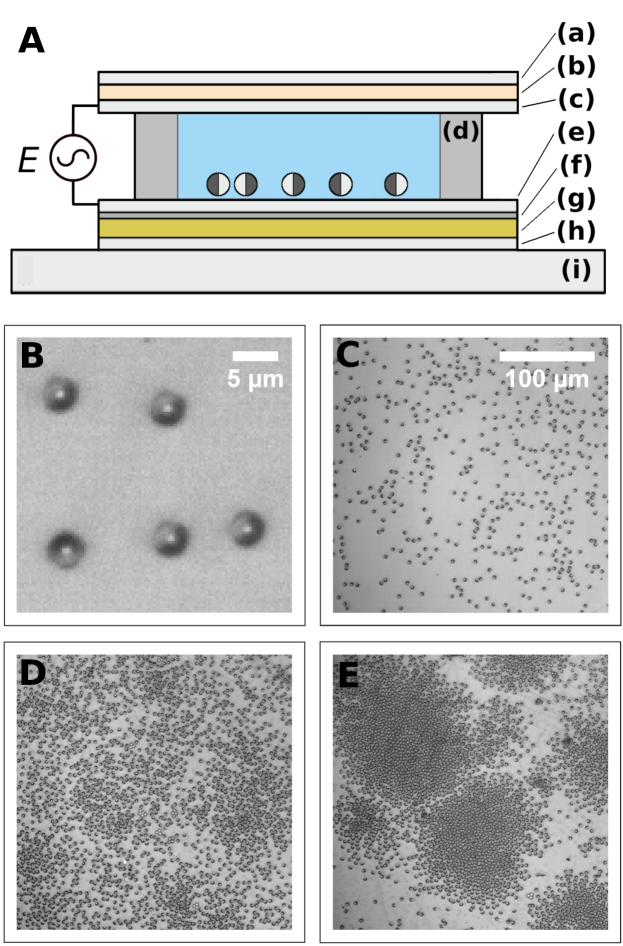
Figure 1: Experimental set-up. (A) Scheme of an observation cell. (a) Cover slip, (b) ITO electrode, (c) 25 nm silica, (d) spacer with UV glue, (e) 25 nm silica, (f) 5 nm chromium, (g) 80 nm gold, (h) cover slip and (i) glass slide. (B-E) Snapshots of the experimental system. (B) Zoom on five electrophoretic Janus particles where the two hemispherical caps are clearly seen. When an electric field, $E$, is applied perpendicular to the substrate particles orient themselves in such a way to maximize the magnitude of their induced dipoles, the equator that separates the caps is perpendicular to the substrate, confining the movement to $2$D. Depending on the intensity of the electric field, $E$, and the area fraction, $\phi$, different phases are observed: (C) Gas phase (dilute, $\phi=0.10$, $E=727$ Vcm^-1). (D) Liquid-like phase ($\phi=0.29$, $E=181$ Vcm^-1, activity is too low to phase separate). (E) Interrupted phase separation ($\phi=0.29$, $E=363$ Vcm^-1).

II The Graph Neural Network

To start with, the systems we focus on are in the overdamped regime (Brownian dynamics), where inertia is neglected and viscous forces dominate the dynamics. In this limit, the deterministic equation of motion for particle $i$ simplifies to $\dot{\vec{x}}_{i}\propto\vec{F}_{i}$. For this reason, in the following, we will alternatively refer to forces or velocities, since they are related by the Stoke’s law (see appendix C.2 for more details). All forces acting on each particle – represented by $\vec{F}$ – can be of different nature, such as inter-particle interactions, external conservative fields or active forces. Active forces model different mechanisms of self-propulsion, where particles (such as bacteria or Janus particles) extract energy from the environment and use it for self-propelling. Our goal is to disentangle and learn the different forces acting on the particles from their trajectories. These forces can be later used to predict the dynamics of a new group of particles or to understand the physics governing the dynamics of the system.

Learning to predict the dynamics of active particles can be achieved using a broad range of machine-learning models. For example, one could use a Deep Neural Network (DNN) that takes the positions and internal orientations of all particles as inputs ($3N$ degrees of freedom for a $2$D system) and predicts velocities ($2N$ degrees of freedom for the same 2D system). Training this model would be very challenging, and even if successful, would lead to a highly-dimensional nonlinear function $\vec{f}(\vec{c}_{1},\dots,\vec{c}_{N}):\mathbb{R}^{3N}\to\mathbb{R}^{2N}$, where $\vec{c}_{i}$ is the coordinate vector of particle $i$ (position and orientation). Even though this network could predict the system’s dynamics, it presents two main drawbacks: (i) it cannot be easily applied to a system with a different (varying) number of particles, (ii) there is no guarantee (probably not possible in most cases) that we can use this method to disentangle and extract all forces controlling the dynamics of individual particles, e.g. the active and inter-particle forces.

Graph Neural Networks, on the other hand, are combinations of DNNs applied sequentially on a graph. Their modularity and the possibility of adding inductive biases – a priori assumptions that simplify the model – make them easier to train. By design, the same GNN can be applied to systems of different number of particles, and after training one can easily extract the forces acting on single particles. In our case, we use an edge and a node function (two neural networks): each node on the graph corresponds to one particle in the system and edges represent the interactions between two particles. The edge function encodes the information of pairs of particles (e.g., their mutual distance), and will lead to the estimate of the two-body force. Whereas the node function takes as input the coordinates of a particle and the output of the edge function (see appendix C.2 for more details) and will lead to the estimate of the one-body forces, such as the active force. For each time frame, a new graph is created (eventually with a different number of nodes), and the GNN (defined by the functions applied to the nodes and edges) is applied.

Compared to the naive approach of adopting a single, huge neural network, trained over all data, the GNN model is less complex. The lower complexity is made possible by some crucial, physically justified assumptions: a) the same forces control the dynamics of all particles (particles are identical), and b) many-body interactions are neglected, only one-body (active and drag forces) and two-body forces are considered, although these assumptions can be relaxed if necessary. The training of the GNN goes as follow, first we apply the edge function $\vec{\xi}(\vec{c}_{i},\vec{c}_{j})$ to a node $i$ and each of its $j$-neighbors (each pair of particles constitutes an edge, $ij$). Then, we sum up these outputs and we feed the result to the node function, $\vec{\psi}$, along with the coordinates of the $i$-th node, $\vec{c}_{i}$. The output of the node function is the predicted velocity for the $i$-th particle $\vec{v}_{i}^{p}$. Mathematically,

$$\vec{v}_{i}^{p}\equiv\vec{\psi}\left(\vec{c}_{i},\sum\limits_{d_{ij}<\Gamma}\vec{\xi}(\vec{c}_{i},\vec{c}_{j})\right)$$ (1)

where $d_{ij}$ is the Euclidean distance between particles $i$ and $j$. Since we tackle systems of thousands of particles and the number of edges in a fully connected graph scales as $\sim N^{2}$, we introduce edges in our graph only between pairs of particles such that $d_{ij}<\Gamma$ and the number of edges scales now as $\sim N$. This process is repeated for each particle in the system, using the same node and edge functions. The training is performed by minimizing the difference between the predicted and ground-truth velocities. In this case, we use the loss function:

$$\mathcal{L}=\sum\limits_{i}|\vec{v_{i}}-\vec{v_{i}}^{p}|.$$ (2)

In figure 2, we show a diagram of the basic idea behind the GNN workflow, that we will name ”ActiveNet”.

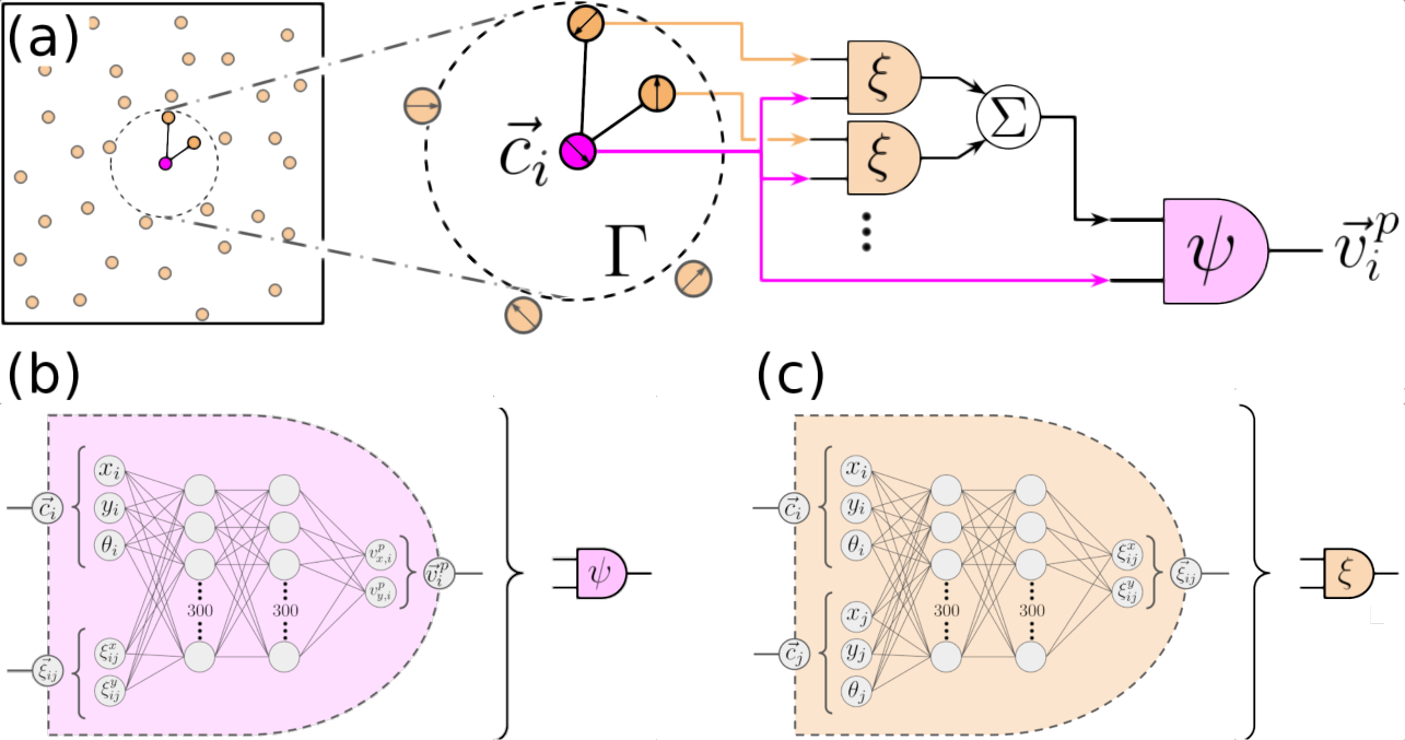
Figure 2: Predicting the dynamics of active particles with a Graph Neural Network (ActiveNet) while learning the functional form of the active and inter-particle forces. (a) ActiveNet is formed by a node function $\vec{\psi}$ (in pink) and an edge function $\vec{\xi}$ (in orange). Function $\vec{\xi}$ takes the coordinates $\vec{c}$ of two particles and, after training, it outputs a linear transformation of the two-body force acting between them. Function $\vec{\psi}$ takes the coordinates of particle $i$ and the sum of the outputs of $\vec{\xi}$ for all the edges $ij$ such that $|\vec{r}_{i}-\vec{r}_{j}|<\Gamma$. After training, the output of $\vec{\psi}$ ($\vec{v}_{i}^{p}$) is the predicted velocity of particle $i$ (acceleration in the case of underdamped dynamics). Applying ActiveNet to all particles in the system (the graph) provides all the predicted velocities. During the learning process the internal parameters of $\vec{\xi}$ and $\vec{\psi}$ are optimized so that all the $\vec{v}_{i}^{p}$ approach the ground-truth velocities. Both the node (b) and edge (c) functions are neural networks with two hidden layers of 300 neurons and the appropriate input and output dimensions.

Note that this scheme applies also to the case of underdamped dynamics, where ActiveNet outputs the predicted acceleration instead of the predicted velocity of the particle. In this case, velocities can be used as inputs to $\vec{\xi}$ and $\vec{\psi}$, making it possible to learn forces that depend on velocities. Once ActiveNet is trained, we use $\vec{\xi}$ and $\vec{\psi}$ to extract the inter-particle and active forces that it has learned (see the appendix C.2 for more details). Note that the two-body force learned for distances larger than $\Gamma$ will be meaningless since there is no data there. In practice, we choose a small $\Gamma$ value for a first training, and train again the model with larger values of $\Gamma$ until we see that the inter-particle force term goes to zero. Thus, we gain no information by increasing $\Gamma$ even further.

III Results

III.1 ActiveNet correctly learns the forces in simulations of active particles

In the case of overdamped dynamics, our approach is actually a fitting of the active and conservative forces (velocities) by the two neural networks composing ActiveNet, such that the observed collective dynamics is recovered, and the forces controlling the particles’ dynamics are learnt. This section validates our method for its use in experimental suspensions of active particles. We test our model first using simulations of a two-dimensional suspension of active Brownian particles (detailed in section B). We choose to study spherical self-propelled particles with a force of constant modulus acting in the direction of their orientation measured with respect to the horizontal axis ($\theta$). Particles interact with each other via different two-body potentials. The internal orientation of every particle changes according to a diffusion equation, whereas the overdamped translational equations of motion for all particles determine their trajectories. To demonstrate that ActiveNet can be extended beyond active Brownian particles, we also simulate active particles whose translational equations undergo Langevin (instead of Brownian) dynamics, see appendix B for more details.

We perform simulations on very different systems, ranging from active Brownian repulsive particles in a MIPS phase, to active Brownian attractive particles in a dynamic clusters phase, to a gas of active repulsive particles, either undergoing Brownian or Langevin dynamics. Figure 3 shows the two-body forces ($|G_{ij}^{p}|$) and the active force ($|F^{p}|$) that ActiveNet learns (continous lines) after training making use of trajectories generated in simulations where particles interact with different potentials, attractive or repulsive, and present different levels of activity. In the case of active particles undergoing Langevin dynamics, besides the two-body and active forces, ActiveNet also learns the drag force acting on each particle, which we include as panel (d) in figure 3. For comparison, we also show the ground-truth forces imposed in the simulations as dashed lines.

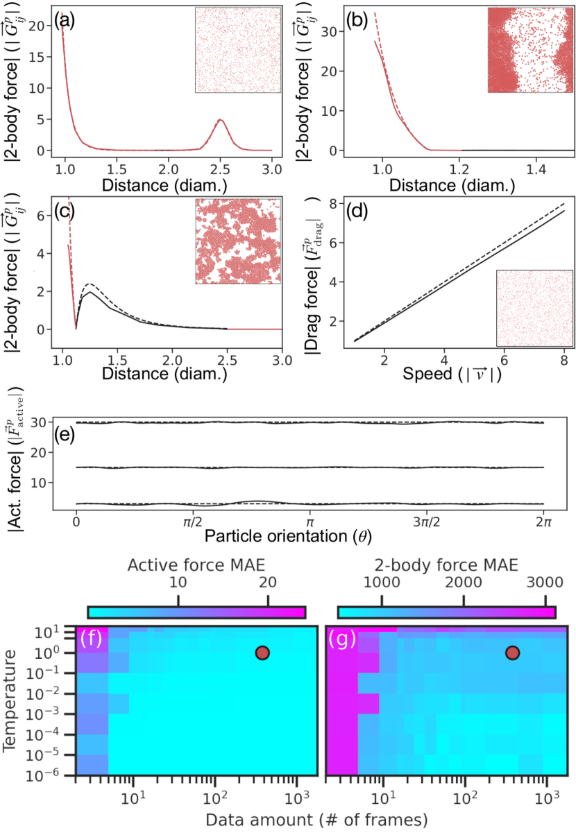
Figure 3: ActiveNet can learn the forces present in simulations of active particles from their trajectories. To test ActiveNet, we perform computer simulations on two-dimensional suspensions of different systems. Panels (a), (b) and (c) illustrate the two-body force versus the distance between two particles in several cases: (a) shows the case of a shoulder-like potential for active particles in a gas phase ($F_{p}=15$); panel (b) corresponds to active repulsive (WCA-like) Brownian particles in a MIPS phase ($F_{p}=30$); and panel (c) displays the case of active attractive (Lennard-Jones) Brownian particles in a dynamic cluster phase ($F_{p}=3$). Panel (d) shows the drag force versus the particle’s velocity for active repulsive (WCA-like) particles undergoing underdamped Langevin dynamics in a gas phase ($F_{p}=3$). In all panels the ground-truth force (the one inputted in the simulations) is plotted with dashed lines, whereas the force predicted by ActiveNet is plotted with continous lines, in both cases repulsive interactions are plotted in red and attractive in black. See methods for more details. Insets to panels (a), (b), (c) and (d) show snapshots of the corresponding simulations. Panel (e) depicts the magnitude of the active force acting on each particle versus the angle $\theta$, either enforced in the simulations (dashed line) or learned from ActiveNet as in (11) (continuous line). The lowest lines correspond to $F_{p}=3$, the middle lines to $F_{p}=15$ and the top lines to $F_{p}=30$. Panels (f) and (g) display the Mean Absolute Error for the predicted active and 2-body forces as a function of the temperature of the simulation and the amount of data used for training the network (measured as the number of frames, each containing $2\,500$ particles). The red dot shows the values of these parameters used for panels (a-e). Additional details can be found in the appendix sections B and C.3 (figure 6).

In the overdamped cases, for each simulation ActiveNet is trained using $380$ snapshots of $2\,500$ particles. ActiveNet adopts as input the positions and orientations of all particles in each frame, and learns to predict the correct velocities. In this process, the edge function learns the conservative force between any pair of particles (up to a linear transformation) whereas the node function learns the active force acting on each particle. In the case of underdamped Langevin dynamics, ActiveNet adopts as an input positions, orientation and velocities of all particles in each frame, and learns to predict the correct accelerations. In this process, the edge function learns the conservative force between any pair of particles (up to a linear transformation), as in the Brownian case. However, the node function learns not only the active force acting on each particle but also the drag force on each particle. See appendix sections B and C.2 for further details.

Figure 3 presents some of the most challenging cases for ActiveNet. (i) A dilute suspension (gas phase) of particles interacting via a repulsive force characterised by two length scales derived from a shoulder potential, panel (a). (ii) A dense suspension of particles interacting via a purely repulsive Weeks-Chandler-Anderson (WCA) [83] interaction with high activity, panel (b). Particles undergo a motility induced phase separation (MIPS) and ActiveNet has to learn a repulsive force even though the system phase separates due to particles’ activity. (iii) A dilute suspension of particles interacting via an attractive Lennard-Jones interaction with low activity, panel (c). Particles form “dynamic” clusters that jiggle and drift, where very few particles explore different local structures, making it harder for ActiveNet to learn the two-body forces. (iv) A dilute suspension of particles interacting via a purely repulsive Weeks-Chandler-Anderson (WCA) [83] potential with low activity, panel (d). Particles follow Langevin dynamics (differently from case (i), where active repulsive particles undergo Brownian dynamics). In all cases, ActiveNet is able to correctly learn the active, two-body and drag forces. Interestingly, the two-body force learned by ActiveNet deviates from the imposed force for short distances, when the imposed numerical value is larger than the active force present in the system. This is because the dominant short-range repulsive force leads to a lack of data at those distances. In system (iii), ActiveNet slightly underestimates the two-body force. This is likely due to the fact that, at low activities, the two-body forces change within a shorter time scale than in (i), (ii) or (iv), leading to a reduction in the correlation between the numerical (average) velocity and the instantaneous force we aim to learn. Moreover, in the Langevin dynamics (case (iv)), ActiveNet can also learn the drag force (from particles’ accelerations). We conclude that ActiveNet is able to learn ground-truth forces across several orders of magnitude under a wide set of conditions.

III.2 ActiveNet learns active and two-body forces in experiments of electrophoretic Janus particles

We have performed experiments in a quasi-2D system of induced-charge electrophoretic self-propelled Janus colloids [4, 6, 5], (see the details in section A). Due to the AC field, the colloids self-propel and exhibit inter-particle interactions as a result of their electric polarization. Most experiments with passive colloids have been modeled in the overdamped (Brownian) regime[84, 84, 85]. For active colloids, hydrodynamics is often considered to be relevant for unraveling particles’ motion. Photocatalitic TiO₂-functionalised Janus microswimmers, self-propelling when exposed to ultra-violet light [86], have shown complex two- and three-dimensional motion, controlled by the colloids’ hydrodynamic interactions with the glass substrate [87]. In [88], the authors studied half-gold-coated TiO₂ particles, whose direction of motion could be reversed by exploiting the different photocatalytic activities on both sides. The reversal in propulsion direction changed the hydrodynamic interaction from attractive to repulsive, qualitatively described by a minimal hydrodynamic model. On the other hand, it is quite frequent to map experiments on active colloids onto simulation results of active Brownian particles (neglecting, to a first approximation, hydrodynamics). Just to give a few examples, experimental results on active colloids have been compared to numerical results on active overdamped Brownian particles in Ref. [89] (Janus Platinum-Polysterene catalytic microswimmers with tunable buoyant weight), in Ref. [90] (light-activated microswimmers, with an inserted hematite), in Ref. [91] (silica spheres half-coated with a carbon layer in a critical fluid), and in Refs. [92] and [6] (induced-charge electro-phoretic colloids in an ac field). In the latest work[6], the authors employed the same experimental set-up as the one we have used here. Furthermore, we have also estimated the Reynolds number of our experimental system and proved it was $\ll 1$. All this supported our assumption that hydrodynamics was not going to dominate either the dynamics or the strength of electrostatic interactions between dipoles (as already suggested by the previous authors studying the same system). Thus, to a first approximation, in the dilute regime and for low electric field amplitudes, we train ActiveNet assuming overdamped dynamics.

Without ActiveNet, extracting the expressions for the active and two-body forces from the collective dynamics of the particles would be extremely hard. ActiveNet allows us to tackle this problem from a completely different point of view: from particles’ positions and orientations, ActiveNet fits the active and two-body forces that best predict the particles’ velocities.

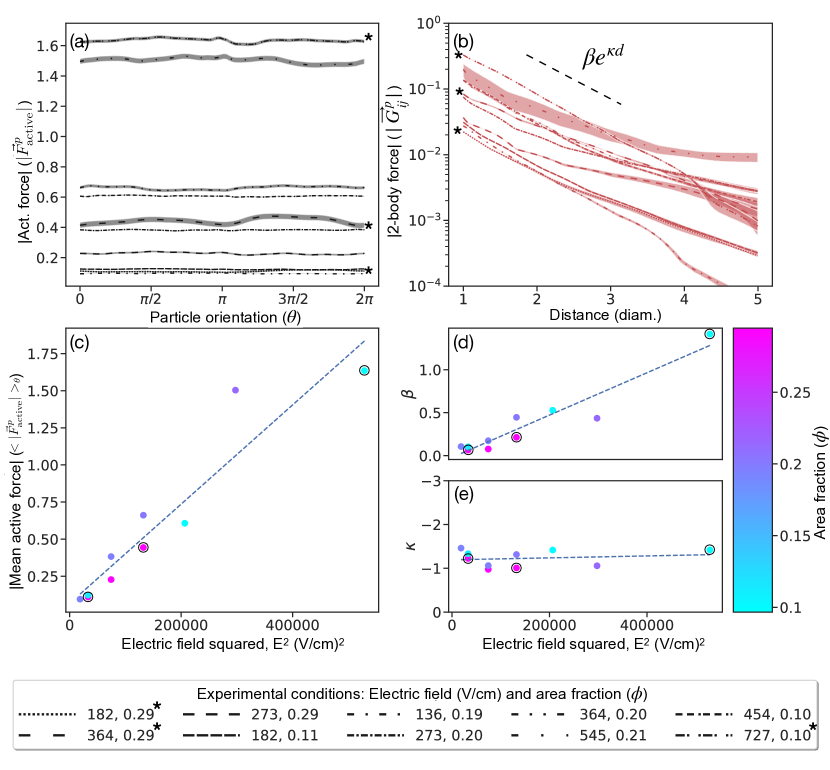
Figure 4: ActiveNet can learn the active and inter-particle forces in an experiment of electrophoretic Janus particles where activity is controlled by the magnitude of the electric field ($E$). In panels (a) and (b), the ten different series of data (lines with different styles) represent ten different systems, each characterised by a pair of values of the electric field (E) and the area fraction ($\phi$), as reported in the legend, below the four panels. Note that three values of $(E,\phi)$ correspond to the snapshots shown in figure. 1, we have marked them with black asterisks in panels (a) and (b) and black circumferences in panels (c), (d) and (e). In panels (a) and (b) we train ten instances of ActiveNet for each dataset with different initial seeds, lines correspond to the average result and the shadows around the lines mark the estimated uncertainty (error bar) by means of the standard deviation. Panel (a) displays the magnitude of the active force versus the particle’s orientation. All lines show horizontal behavior indicating the absence of a preferred direction in the system. Panel (b) displays the modulus of the inter-particle force versus the distance between two particles. All forces are repulsive (red lines) and they approximately follow exponential decays, $\beta e^{\kappa d}$. The black dashed line does not correspond to any particular fit and is included for visualization. Panel (c) reports the average value of the active force in panel (a) versus $E^{2}$. The dashed line is a linear fit to the points and indicates that the active force is proportional to $E^{2}$. Panels (d) and (e) show $\beta$ and $\kappa$ ($\beta e^{\kappa d}$, $d\in[1,3]$) for all the lines in panel (b) versus $E^{2}$ (individual fits are not plotted in panel (b)). From panel (d), $\beta$ scales as $E^{2}$, the dashed blue line represents a fit to the data. Panel (e) shows that, $\kappa$ does not depend on $E$ or $\phi$. Its value fluctuates between $-1$ and $-2$ leading to a length scale of the order of one particle diameter. The color of the points in panels (b), (d) and (e) correpond to the area fraction ($\phi$, see colorbar).

For simplicity, we build ActiveNet assuming that the active force depends on the orientation of the particle and the two-body force depends on the distance between pairs of particles (see appendix C.1 for more details). We train ActiveNet with data extracted from ten different experiments, performed at different values of both electric field and area fraction, as reported in figure. 4 (the values are explicitly indicated in the legend). Each time, ActiveNet is randomly initialized before the training started. Depending on the amount of data gathered in each experiment, we use $50-100$ snapshots containing approximately $1\,000-6\,000$ particles each. Figure 4 (a) presents the modulus of the active force as a function of particles’ orientation ($\theta$). Approximately horizontal lines indicate that ActiveNet is learning an active force with a constant modulus and no preferred direction. In this panel, (as well as in panel (b), we mark by shadows around the lines the estimated uncertainties (error bars) for the predictions. Each data point corresponds to the average of an ensemble of ten ActiveNet models, trained with the same data and, as mentioned in the introduction, with different initial seeds; the error bar is the standard deviation of the predictions. We notice that the error bars are small compared to the absolute values of the predicted values and support our observation of no preferred direction. We calculate the average value of each line and plot it in panel (c) as a function of the square of the electric field amplitude. Points are scattered along a straight line, leading to the expected [6] relation $\vec{F}^{p}\sim CE^{2}$, see appendix C.2. Moreover, points seem to follow different straight lines depending on their area fraction, what leads to a relation $\vec{F}^{p}\sim C(\phi)E^{2}$. A possible explanation is that in our experiments a different sample cell was used for each area fraction; although these cells are ideally equivalent, small differences in the spacing between the confining walls could lead to systematic errors in the observed prefactor ($C(\phi)$). However, more work is needed to resolve the real cause of this dependence. It is remarkable that ActiveNet seems to be sensitive enough to detect this subtlety.

Figure 4 (b) shows the two-body force , with error bar marked by a shadow, that ActiveNet learns as a function of the distance between two particles. The straight lines in the semi-log plot indicate an exponential decay. Low area fraction experiments ($\phi\sim 0.1$) lead to very clear and almost parallel straight lines, whereas experiments at higher area fractions present more variability. The experiments that combine high electric field and high area fraction present an interrupted MIPS phase (see figure. 1). Thus, it is reasonable to assume that it will be harder for ActiveNet to learn the two-body interactions in those cases: here, particles are closer together and many-body interactions will play a more pronounced role. We fit each line between $d=1$ and $d=3$ to an expression of the form $\beta e^{\kappa d}$ (fits not shown in the plot). Panels (d) and (e) show the best fit for $\beta$ and $\kappa$, for each experiment. The prefactor of the exponential decay ($\beta$) scales also as $E^{2}$, consistent with the a screened electrostatic interaction [93, 94], since the polarization in each colloid is proportional to $E$. On the other hand, $\kappa$ does not seem to depend on $E$ or on area fraction and has an approximate value of $-1.2$ diameter^-1, uncovering a length scale for this interaction of approximately one particle diameter.

IV Discussion and future work

Our work shows the potential that applying deep learning methods with inductive biases (a priori assumptions) has when studying the collective dynamics of suspensions of active colloidal particles. The most important a priori assumptions we considered were that all particles followed the same local rules (edge and node functions) and that many-body interactions could be neglected. With these assumptions, ActiveNet was not only able to predict the system’s dynamics, but could be directly used to uncover forces acting on active particles. We validated our approach by means of numerical simulations in the under and overdamped regime, where we had complete control over the active and conservative forces. We were able to extract the correct expressions for the forces in cases with different levels of activity and different two-body interaction potentials, including forces that depend on velocities – such as the drag force –, which opens the possibility of using ActiveNet to learn more complex hydrodynamic forces. In the case of experiments with electrophoretic Janus particles, ActiveNet found an active force proportional to $E^{2}$, in agreement with previous studies [95]. Furthermore, ActiveNet was sensitive enough to detect subtle differences showing a dependency on area fraction. Finally, ActiveNet revealed that particles in these experiments were interacting via a pure repulsion, decaying as an exponential with a length scale ($\kappa^{-1}$) that did not depend neither on area fraction nor electric field, and a prefactor that scaled as $E^{2}$. This force is consistent with a screened electrostatic interaction between the colloids. Contrary to the case of numerical simulations, the two-body force learned from experimental data started deviating from the described behavior when interrupted MIPS phases developed, suggesting that many-body interactions might start playing an important role in such cases.

We believe that ActiveNet can be directly applied to other suspensions of active particles. For example, it would be interesting to use this approach to distinguish between forces present in systems of healthy or pathological living cells (similarly to [96]), which may ultimately lead to a diagnostic tool. ActiveNet could also be applied to passive systems. In particular, since ActiveNet uses particles’ dynamics and not structural information, it could be especially useful when a system of passive colloids is out-of-equilibrium (due to a particular initial condition or to external driving). On the theoretical side, we are working on training a new version of ActiveNet to account for many-body interactions. For this purpose, one might consider including a new function in the GNN. Moreover, a symbolic regression will help understanding the analytic expression for the inter-particle interactions [97, 98]. Additionally, we plan to test if the training of these GNNs can be improved using a dynamical change of its loss function landscape [99], considering a cutoff ($\Gamma(\tilde{t})$) that changes during training. In cases where the dynamics of the system changes during the observation time, it will be interesting to understand how the architecture of ActiveNet affects the capability of forgetting or transferring previous knowledge to new conditions [100, 101].

To conclude, our work opens up new avenues for understanding systems of active particles. Our approach leads to a ready-to-use tool for experimentalists to learn the forces present in their systems . The extracted forces will shine a light on the physics underlying experimental systems, which in turn could lead to novel numerical and analytical models, undoubtedly leading to new predictions in the field of active matter.

Authors M.R.-G. and C.M.B.G. contributed equally to this work.

Appendix A Experimental details

We used silica particles with a diameter of $4.28\text{\,}\mathrm{\SIUnitSymbolMicro m}$ to create Janus particles. We first deposited them onto cleaned glass slides with a resulting area fraction of $0.1$ and we left the solvent to evaporate. They were then coated with $50\text{\,}\mathrm{nm}$ of titanium by vapour deposition, then coated with $15\text{\,}\mathrm{nm}$ of silica. These particles were then removed by gentle sonication into a NaCl $0.1\text{\,}\mathrm{mmol}\text{\,}{\mathrm{dm}}^{-3}$ solution. The sample cell was built with an upper electrode: we used $15$-$30\text{\,}\mathrm{\SIUnitSymbolOhm}\text{\,}{\mathrm{cm}}^{-1}$ ITO cover slips from Diamond Coatings Ltd coated in $25\text{\,}\mathrm{nm}$ silica by vapour deposition. We used a $80\text{\,}\mathrm{nm}$ gold electrode with $5\text{\,}\mathrm{nm}$ of chromium and $25\text{\,}\mathrm{nm}$ of silica for the substract in contact with particles. Specac Omni Cell spacers from Merck of a width of $60\text{\,}\mathrm{\SIUnitSymbolMicro m}$ were used with Norland optical UV glue to separate the electrodes. This left a gap of $110(010)\text{\,}\mathrm{\SIUnitSymbolMicro m}$ between the electrodes. An alternating square potential at $8\text{\,}\mathrm{kHz}$ and varying amplitude was passed through a signal generator creating a field perpendicular to the observation plane. A sketch of the experimental set-up is shown in figure 1. Recordings were made with a $4.2MPix$ XIMEA camera at a constant framerate ($<10.3fps$) in a reflection microscopy setup. To this end, a BS013 $50$:$50$ beam splitter from Thorlabs was used with an Olympus UPLXAPO 20X oil immersion Objective. Particles were detected with a custom algorithm and tracked with software by J. C. Crocker [104].

Electro-phoretic Janus particles have tunable behaviours. Nishiguchi et al. [95] showed that the direction and speed of the particles could be changed by increasing the frequency of the ac electric field. Zhang et al. and Yan et al. also demonstrated that the electrostatic interactions between the induced charges in the particles change and invert through a similar change in electric field frequency [5, 6]. In our work, we selected the electric field and particle properties such that we avoided the regime where forces between the metal and dielectric cap were attractive, aiming for purely repulsive forces through which we could form MIPS. The typical conductivity of ions in solution, given that they interact with a solvent and other ions, is typically lower than that of electrons in the metallic cap. Because of this, the velocities of our particles are quenched when the frequency of our electric field enters the region of 1M Hertz and a visible reduction occurs in the kHz range. We therefore hypothesize that the screening effects of the ions and double layers, which are induced by the induced polarization of the particle, are more isotropic than if the ions could move in sync with the AC field.

Appendix B Numerical simulations details

We simulated a two-dimensional suspension of active particles undergoing either Brownian or underdamped Langevin dynamics. The numerical simulations of the active Brownian particles consist of $N=2\,500$ circular particles with diameter $\sigma$ in a two-dimensional box of size $L\times L$ (with periodic boundary conditions). The value of $L$ has been set to obtain the desired total number density $\rho=\frac{N}{L}\in\{0.1,0.6\}$. As in ref. [105], we use the total density of the system instead of the packing fraction, since a particle’s diameter (necessary for computing the packing fraction) might not be uniquely defined due to particles activities (and cannot be estimated via the Barker and Henderson’s approach [106]). To simulate active Brownian particles, we perform Brownian dynamics simulations, with an in house modified version of the LAMMPS [107] open-source package, for $T_{\text{sim}}=10^{7}$ timesteps with $dt=10^{-5}$ (reduced units) following ref. [108]. We simulate an overdamped system through equations of motion for the position $\vec{r}_{i}$ and orientation $\theta_{i}$ of the $i$-th active particle, which can be written as:

$$\dot{\vec{r}}_{i}=\frac{D_{t}}{k_{\textrm{B}}T}\left(-\sum_{j\neq i}\nabla V(r_{ij})+F_{p}\,\vec{n}_{i}\right)+\sqrt{2D_{t}}\,\vec{\xi}_{i},$$ (3)

$$\dot{\theta}_{i}=\sqrt{2D_{r}}\,\xi_{i,\theta},$$ (4)

where $V(r_{ij})$ is the inter-particle pair potential, $k_{B}$ the Boltzmann constant, $T$ the absolute temperature, $F_{p}$ a constant self-propulsion force acting along the orientation vector $\vec{n}_{i}$, which forms an angle $\theta_{i}$ with the positive $x$-axis, $D_{t}$ and $D_{r}$ are the translational and rotational diffusion coefficients. Furthermore, the components of the thermal forces $\vec{\xi}_{i}$ and $\xi_{i,\theta}$ are white noise with zero mean and correlations $\langle\xi^{\alpha}_{i}(t)\xi^{\beta}_{j}(t^{\prime})\rangle=\delta_{ij}\delta_{\alpha\beta}\delta(t-t^{\prime})$, where $\alpha,\beta$ are the $x$, $y$ components, and $\langle\xi_{i,\theta}(t)\xi_{j,\theta}(t^{\prime})\rangle=\delta_{ij}\delta(t-t^{\prime})$. $D_{t}=k_{B}T/\gamma=0.01$, with $\gamma=1$, $D_{r}\in\{0.25,1.0\}$ and $F_{p}\in\{3,15,30,60,120\}$ in order to achieve a wide range of phases, although we only included three cases in the main text.

Next, we simulate active particles undergoing underdamped Langevin dynamics with the LAMMPS [107] open source package, for $T_{\text{sim}}=10^{7}$ timesteps with $dt=10^{-3}$ (reduced units). The equations of motion for the position $\vec{r}_{i}$ and orientation $\theta_{i}$ of the $i$-th active particle can be written as:

$$m\dot{\vec{v}}_{i}=-\sum_{j\neq i}\nabla V(r_{ij})+F_{p}\,\vec{n}_{i}-\gamma_{t}\vec{v}_{i}+\sqrt{2\gamma_{t}k_{B}T}\,\vec{\xi}_{i},$$ (5)

$$\dot{\theta}_{i}=\sqrt{2D_{r}}\,\xi_{i,\theta},$$ (6)

where $V(r_{ij})$ is the inter-particle pair potential, $F_{p}$ a constant self-propulsion force acting along the orientation vector $\vec{n}_{i}$ which forms an angle $\theta_{i}$ with the positive $x$-axis, $\gamma_{t}$ the translational friction coefficient, and $D_{r}=k_{B}T/\gamma_{r}$ the rotational diffusion coefficient. Furthermore, the components of the thermal forces $\vec{\xi}_{i}$ and $\xi_{i,\theta}$ are white noise with zero mean and correlations $\langle\xi^{\alpha}_{i}(t)\xi^{\beta}_{j}(t^{\prime})\rangle=\delta_{ij}\delta_{\alpha\beta}\delta(t-t^{\prime})$, where $\alpha,\beta$ are the $x$, $y$ components, and $\langle\xi_{i,\theta}(t)\xi_{j,\theta}(t^{\prime})\rangle=\delta_{ij}\delta(t-t^{\prime})$. We simulated this underdamped system with $N=3600$ active particles with $F_{p}=5$ in a rectangular box of side $L=600$ corresponding to a density of $\rho=0.01$. The temperature was fixed to $k_{B}T=1$ with a traslational and rotational friction coefficients of $\gamma_{t}=1$ and $\gamma_{r}=10/3$ respectively, consistent with the rotational diffusivity of spherical particles [79].

Throughout our study, we considered three interaction potentials between particles ($V(r_{ij})$, see figure 5): the truncated and shifted Lennard-Jones potential (LJ) and two repulsive potentials, WCA [83] and a shoulder potential [109]. The short-range attractive Lennard-Jones potential obeys the following equation

$$V_{\text{LJ}}(r)=4\epsilon\left[\left(\dfrac{\sigma}{r}\right)^{12}-\left(\dfrac{\sigma}{r}\right)^{6}\right]$$ (7)

where $r$ is the center-to-center distance, $\sigma$ is the particle diameter and $\epsilon$ is the depth of the minimum, that quantifies the attraction strength. The truncated and shifted LJ potential is accomplished by truncating $V_{\text{LJ}}$ to zero after a given cutoff ($r_{\text{cut}}=2.5\sigma$), and shifting it up to recover continuity at $r=r_{\text{cut}}$.

$$V_{\text{TSLJ}}(r)=\left\{\begin{array}[]{lcl}V_{\text{LJ}}(r)-V_{\text{LJ}}(2.5\sigma)&,&r<2.5\sigma\\ 0&,&r\geq 2.5\sigma\end{array}\right.$$ (8)

The repulsive WCA potential can be written as a truncated LJ potential setting $r_{\text{cut}}=r_{\text{min}}=2^{1/6}\sigma$ (the distance to the potential minimum), and shifting it up to recover continuity at $r=r_{\text{cut}}$

$$V_{\text{WCA}}(r)=\left\{\begin{array}[]{lcl}V_{\text{LJ}}(r)+\epsilon&,&r<2^{1/6}\sigma\\ 0&,&r\geq 2^{1/6}\sigma\end{array}\right.$$ (9)

where $V_{\text{LJ}}(r_{\text{min}})=-\epsilon$. Finally, the repulsive shoulder potential is characterized by two different length scales: a repulsive hard core and a soft repulsive shell around each particle (see figure 5) According to [109]

$$V(r)=\epsilon\left(\frac{\sigma}{r}\right)^{n}+\frac{1}{2}\,\varepsilon_{s}\,\left\{1-\tanh{\left[k_{0}\,\left(r-\sigma_{s}\right)\right]}\right\}$$ (10)

where $\sigma$ is the hard core diameter, $\epsilon_{s}$ and $\sigma_{s}$ are the height and width of the repulsive shoulder, respectively, $n$ affects the stiffness of the repulsive core and $k_{0}$ describes the steepness of the shoulder decay (figure 5). Following ref. [109], we use the following parameters: $n=14$ and $k_{0}=10/\sigma$ and $\sigma_{s}=2.5$.

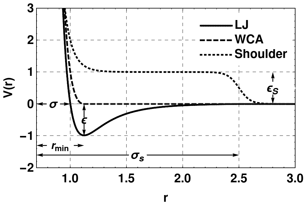
Figure 5: Two-body potentials used in the numerical simulations. The Lennard-Jones potential describes short-range attraction between particles. WCA and shoulder potentials lead to purely repulsive forces between particles. ActiveNet can learn the inter-particle passive force derived from all three potentials.

In our simulations we set $\epsilon=\sigma=m=1$. All quantities are expressed in reduced LJ units, $r^{*}=r/\sigma$, $\tau^{*}=\tau\sqrt{\epsilon/m\sigma^{2}}$, $F^{*}=\sigma F/\epsilon$ and $U^{*}=U/\epsilon$ and $k_{B}=1$. Throughout the manuscript we drop the asterisks to avoid cluttering all equations.

In the case of Brownian dynamics, to train our neural network, we use the position and orientation of all particles at different times as input data and the velocities as the variables that the GNN should reproduce at its output. At a time $t$ we calculate the velocities as $(\vec{x}(t+\Delta t)-\vec{x}(t))/\Delta t$, setting $\Delta t=10$ simulation steps. We have checked that the GNN obtains equivalent results choosing $\Delta t=10,50,100$. In general, using a smaller $\Delta t$ will lead to a better correlation to the instantaneous forces present at $t$ but noiser data (more data may be necessary). On the other hand, a larger $\Delta t$ will lead to a larger signal-to-noise ratio (less amount of data may be necessary) but a degraded correlation with the force we want to learn. In the case of underdamped Langevin dynamics, to train our neural network, we use the position, velocity and orientation of all particles at different times as input data and the accelerations as the variables that the GNN should reproduce at its output. At a time $t$ we calculate the accelerations as $(\vec{v}(t+\Delta t)-\vec{v}(t))/\Delta t$, setting $\Delta t=10$ simulation steps.

Appendix C ActiveNet

C.1 Inductive biases for the edge and node functions

The main assumption when we use ActiveNet is that all the particles follow the same local rules (the edge and node functions) and that we neglect many-body interactions. In this work the edge and node functions are two fully connected deep neural networks with two hidden layers of $300$ units (as shown in the bottom panels of figure 2). In addition to this, we add some extra inductive biases. In the case of experiments, we know there are imperfections in the substrate where few particles might get stuck. Thus, directly providing particles’ positions $(x_{i},y_{i})$ to the edge and node functions would lead ActiveNet to learn this spurious (although real) information. When dealing with the edge function, we directly provide the distance between two particles, instead of feeding ActiveNet with the coordinates and letting it learn $d=\sqrt{(x_{1}-x_{2})^{2}+(y_{1}-y_{2})^{2}}$. Next, we multiply by the unitary vector pointing in the direction connecting the two particles. We also tried providing the distance and the unitary vector as input so that ActiveNet would learn the correct direction of the force: this led to equivalent results.

For the same reason we do not give the position of the particles to the node function, considering as the only input the particle’s orientation $(\cos{\theta},\sin{\theta})$ and the aggregated output of the edge function applied to the pairs ij. In the of underdamped dynamics we also input the velocity ($\vec{v}_{i}$) to the node function. Note that we could have given also the orientation of the particles or the velocities to the edge function—which learns the two-body interaction—, this could have led to learning an interaction depending on alignment or velocities. However, we preferred to consider at this time only the distance between the two particles to prioritize the simplest interpretation of the forces learned by ActiveNet.

C.2 Extracting the active and two-body forces

Probably, the most important feature of ActiveNet is that it allows to learn the forces governing the dynamics of a system of particles, together with a clear physical interpretation of the results. After training, ActiveNet is able to predict the deterministic dynamics, extracting inter-particle and active forces directly from $\vec{\xi}$ and $\vec{\psi}$. As explained in the main text, ActiveNet disentangles the components of the velocities that can be explained through $\vec{\xi}$ and $\vec{\psi}$: to obtain the forces we then use Stokes’ law.

For the simulations of Brownian particles the expressions are dimensionless and forces and velocities take the same values. We extract the learned active force from ActiveNet as:

$$\vec{F}_{\textrm{active}}^{p}(\vec{c})=\vec{\psi}\left(\vec{c},\vec{0}\right).$$ (11)

On the other hand, $\vec{\xi}$ learns the two-body interaction between particles. A key point here is that $\vec{\psi}$ takes as input the sum of several outputs of $\vec{\xi}$. Therefore, if the training is successful and ActiveNet learns the dynamics, $\vec{\psi}$ should only perform a linear transformation on $\sum\limits_{|d_{ij}<\Gamma|}\vec{\xi}(\vec{c}_{i},\vec{c}_{j})$: in other words, $\vec{\xi}(\vec{c}_{i},\vec{c}_{j})$ learns the force between any two particles, up to a linear transformation. In particular, $|\vec{\xi}(\vec{c_{i}},\vec{c_{j}})|$ will be the modulus of the inter-particle force multiplied by an arbitrary constant. The fact that the node function cannot make a nonlinear transformation on the edge function, is the theoretical reason that allows us to disentangle both contributions.

To recover the inter-particle force learned by ActiveNet (plotted in Figs. 3 and 4) we compute the following

$$\vec{\psi}\left(\vec{c}_{i},\vec{\xi}(\vec{c}_{i},\vec{c}_{j})\right)-\vec{F}_{\textrm{active}}^{p}(\vec{c}_{i}),$$ (12)

In principle, this quantity could depend on the orientation of particle $i$, or on the angle that particles $i$ and $j$ form with the horizontal ($\alpha_{ij}$). To extract only the dependence on the distance between the two particles we integrate out both degrees of freedom,

$$\vec{{G}}_{ij}^{p} =$$ (13)

$$=\frac{\int_{0}^{2\pi}\int_{0}^{2\pi}\left[\vec{\psi}\left(\vec{c}_{i},\vec{\xi}(\vec{c}_{i},\vec{c}_{j})\right)-\vec{F}_{\textrm{active}}^{p}(\vec{c}_{i})\right]\textrm{d}\theta\textrm{d}\alpha_{ij}}{2\pi^{2}},$$

In the case of experiments, assuming Brownian dynamics, we obtain forces using Stokes’ law. We multiply the learned velocities (which are of the order of $1$ particle’s diameter s^-1) by $6\pi\eta r\sim 1.7\ 10^{-12}$ N, considering the water viscosity $\eta\sim 10^{-3}$ Pa s and the particle radius $r\sim 4.3\mu$m.

In the case of particles undergoing Langevin dynamics (the underdamped case), we study the trajectories generated by the dimensionless equations described in Sec. B. We consider an edge function analogous to the overdamped case. However, the node function takes now also the velocity of the particle as another input and we train ActiveNet to predict the acceleration of particle i:

$$\vec{a}_{i}^{p}\equiv\vec{\psi}\left(\theta_{i},\vec{v}_{i},\sum\limits_{d_{ij}<\Gamma}\vec{\xi}(\vec{c}_{i},\vec{c}_{j})\right),$$ (14)

where $\theta_{i}$ and $\vec{v}_{i}$ are the orientation and velocity of particle $i$. Once ActiveNet has been trained, and it can correctly predict particles’ accelerations, we take advantage of the isotropicity of the system to compute the active, drag and two-body forces. We integrate out the velocity of the particle to get the active force:

$$\vec{F}_{\textrm{active}}^{p}(\theta)=\frac{\int_{v_{\textrm{min}}}^{v_{\textrm{max}}}\int_{0}^{2\pi}\vec{\psi}\left(\theta,v,\omega_{v},\vec{0}\right)v\textrm{d}v\textrm{d}\omega_{v}}{\pi(v_{\textrm{max}}-v_{\textrm{min}})^{2}},$$ (15)

where $v$ and $\omega_{v}$ represent the modulus and orientation of particle $i$’s velocity. Similarly, we compute the drag force integrating out the internal orientation of the particle:

$$\vec{F}_{\textrm{drag}}^{p}(\vec{v})=\frac{\int_{0}^{2\pi}\vec{\psi}\left(\theta,v,\omega_{v},\vec{0}\right)\textrm{d}\theta}{2\pi}.$$ (16)

Finally, since we are only interested on the dependence of the two-body force on the distance between particles $i$ and $j$, we integrate out the internal orientation and velocity of particle $i$, and also average over the angle between both particles:

$$\vec{F}_{\textrm{2-body}}^{p}(d)=$$ (17)

$$=\frac{\iiint_{0}^{2\pi}\int_{v_{\textrm{min}}}^{v_{\textrm{max}}}\vec{\psi}\left(\theta,v,\omega_{v},\vec{\xi}(d,\alpha_{ij})\right)v\textrm{d}v\textrm{d}\omega_{v}\textrm{d}\alpha_{ij}\textrm{d}\theta}{4\pi^{3}(v_{\max}-v_{\min})^{2}},$$

where $\theta$, $v$ and $\omega_{v}$, represent the internal orientation, speed and orientation of the velocity of particle $i$, whereas $d$ and $\alpha_{ij}$ represent the distance and angle determined by the vector that goes from particle $i$ to $j$.

C.3 Estimating the Mean Absolute Error (MAE)

To estimate the validity range of ActiveNet, we compute the Mean Absolute Error for the predicted active and 2-body forces (eqs. 19 and 18 ) of particles in a two-dimensional dilute suspension of $2\,500$ active repulsive (WCA) Brownian particles characterised by an active force of 30 (reduced LJ units).

$$\text{MAE}(\vec{G}^{p}_{ij})=\frac{1}{N}\sum_{d}|\vec{G}^{p}_{ij}(d)-\vec{F}^{\text{theo}}_{\text{WCA}}(d)|$$ (18)

$$\text{MAE}(F^{p}_{x})=\frac{1}{N}\sum_{\theta}|F_{x}^{p}(\theta)\,-\,|F_{p}|\cos\theta|$$

$$\text{MAE}(F^{p}_{y})=\frac{1}{N}\sum_{\theta}|F_{y}^{p}(\theta)\,-\,|F_{p}|\sin\theta|$$

$$\text{MAE}(\vec{F}^{p})=\sqrt{\text{MAE}^{2}(F^{p}_{x})+\text{MAE}^{2}(F^{p}_{y}})$$ (19)

As shown in the main text, panels (f) and (g) of figure 3 display the Mean Absolute Error for the predicted active and 2-body forces as a function of the temperature and the amount of data used for training the network (measured as the number of frames). The red dot in these panels shows the value of these parameters used for panels (a-e) of the same figure. We now show the evaluation of errors for the two-body force and the active force (figure 6). The solid black curves are the forces learnt by ActiveNet, the dashed curves are the input forces in the simulation: a WCA potential for the pairwise interactions and an isotropic active force with a modulus of 30 in reduced LJ units.

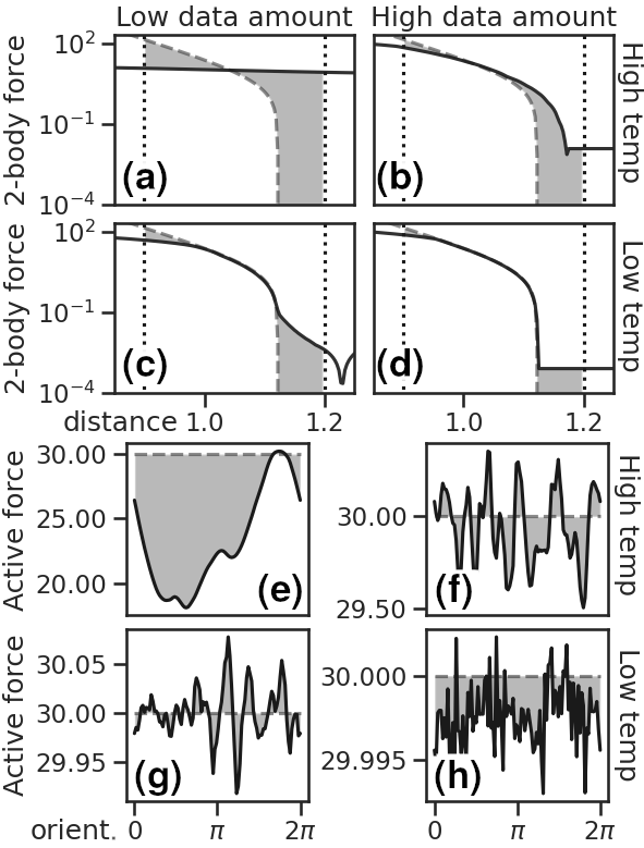
Figure 6: Visual representation of the evaluation of the errors. The solid black curves are forces learnt by ActiveNet, the dashed curves are the ground-truth forces programmed into the simulation. The shaded region in between them is a measure of ActiveNet’s prediction error. The top four panels correspond to the four limit cases for the two-body force: (a) low data – high temperature, (b) high data – high temperature, (c) low data – low temperature and (d) low data – low temperature. The dotted vertical lines show the range in which the error was computed. The bottom four panels (e,f,g,h) correspond to the same cases for the active force.

References

- Ramaswamy [2010] S. Ramaswamy, The mechanics and statistics of active matter, Annu. Rev. Condens. Matter Phys. 1, 323 (2010).
- Vicsek and Zafeiris [2012] T. Vicsek and A. Zafeiris, Collective motion, Physics reports 517, 71 (2012).
- Marchetti et al. [2013] M. C. Marchetti, J.-F. Joanny, S. Ramaswamy, T. B. Liverpool, J. Prost, M. Rao, and R. A. Simha, Hydrodynamics of soft active matter, Reviews of Modern physics 85, 1143 (2013).
- Nishiguchi and Sano [2015] D. Nishiguchi and M. Sano, Mesoscopic turbulence and local order in janus particles self-propelling under an ac electric field, Physical Review E 92, 052309 (2015).
- Zhang et al. [2016] J. Zhang, J. Yan, and S. Granick, Directed self-assembly pathways of active colloidal clusters, Angewandte Chemie 128, 5252 (2016).
- Yan et al. [2016] J. Yan, M. Han, J. Zhang, C. Xu, E. Luijten, and S. Granick, Reconfiguring active particles by electrostatic imbalance, Nat. materials 15, 1095 (2016).
- Van Der Linden et al. [2019] M. N. Van Der Linden, L. C. Alexander, D. G. Aarts, and O. Dauchot, Interrupted motility induced phase separation in aligning active colloids, Physical Review Letters 123, 098001 (2019).
- Zhang et al. [2021] J. Zhang, R. Alert, J. Yan, N. S. Wingreen, and S. Granick, Active phase separation by turning towards regions of higher density, Nat. Physics 17, 961 (2021).
- Trepat et al. [2009] X. Trepat, M. R. Wasserman, T. E. Angelini, E. Millet, D. A. Weitz, J. P. Butler, and J. J. Fredberg, Physical forces during collective cell migration, Nat. physics 5, 426 (2009).
- Volfson et al. [2008] D. Volfson, S. Cookson, J. Hasty, and L. S. Tsimring, Biomechanical ordering of dense cell populations, Proceedings of the National Academy of Sciences 105, 15346 (2008).
- Heinrich et al. [2020] M. A. Heinrich, R. Alert, J. M. LaChance, T. J. Zajdel, A. Košmrlj, and D. J. Cohen, Size-dependent patterns of cell proliferation and migration in freely-expanding epithelia, Elife 9, e58945 (2020).
- Valencia et al. [2021] L. Valencia, V. López-Llorente, J. C. Lasheras, J. L. Jorcano, and J. Rodríguez-Rodríguez, Interaction of a migrating cell monolayer with a flexible fiber, Biophysical Journal 120, 539 (2021).
- Martínez-Calvo et al. [2021] A. Martínez-Calvo, C. Trenado-Yuste, and S. S. Datta, Active transport in complex environments, arXiv preprint arXiv:2108.07011 (2021).
- Tah et al. [2022] I. Tah, D. Haertter, J. Crawford, D. P. Kiehart, C. Schmidt, and A. J.-W. Liu, A minimal model predicts cell shapes and tissue mechanics in the amnioserosa during dorsal closure, Biophysical Journal 121, 263a (2022).
- Heinrich et al. [2022] M. A. Heinrich, R. Alert, A. E. Wolf, A. Košmrlj, and D. J. Cohen, Self-assembly of tessellated tissue sheets by growth and collision, Nat. communication 13, 4026 (2022).
- Ling et al. [2019] H. Ling, G. E. Mclvor, J. Westley, K. van der Vaart, R. T. Vaughan, A. Thornton, and N. T. Ouellette, Behavioural plasticity and the transition to order in jackdaw flocks, Nat. communications 10, 1 (2019).
- Becco et al. [2006] C. Becco, N. Vandewalle, J. Delcourt, and P. Poncin, Experimental evidences of a structural and dynamical transition in fish school, Physica A: Statistical Mechanics and its Applications 367, 487 (2006).
- Bain and Bartolo [2019] N. Bain and D. Bartolo, Dynamic response and hydrodynamics of polarized crowds, Science 363, 46 (2019).
- Palacci et al. [2013] J. Palacci, S. Sacanna, A. P. Steinberg, D. J. Pine, and P. M. Chaikin, Living crystals of light-activated colloidal surfers, Science 339, 936 (2013).
- Mognetti et al. [2013] B. M. Mognetti, A. Šarić, S. Angioletti-Uberti, A. Cacciuto, C. Valeriani, and D. Frenkel, Living clusters and crystals from low-density suspensions of active colloids, Physical Review Letters 111, 245702 (2013).
- Cisneros et al. [2010] L. H. Cisneros, R. Cortez, C. Dombrowski, R. E. Goldstein, and J. O. Kessler, Fluid dynamics of self-propelled microorganisms, from individuals to concentrated populations, in Animal Locomotion (Springer, 2010) pp. 99–115.
- Stenhammar et al. [2015] J. Stenhammar, R. Wittkowski, D. Marenduzzo, and M. E. Cates, Activity-induced phase separation and self-assembly in mixtures of active and passive particles, Physical Review Letters 114, 018301 (2015).
- Murugan et al. [2015] A. Murugan, J. Zou, and M. P. Brenner, Undesired usage and the robust self-assembly of heterogeneous structures, Nat. communications 6, 1 (2015).
- Mallory et al. [2018] S. A. Mallory, C. Valeriani, and A. Cacciuto, An active approach to colloidal self-assembly, Annual review of physical chemistry 69, 59 (2018).
- Narayan et al. [2007] V. Narayan, S. Ramaswamy, and N. Menon, Long-lived giant number fluctuations in a swarming granular nematic, Science 317, 105 (2007).
- Hayakawa [2010] Y. Hayakawa, Spatiotemporal dynamics of skeins of wild geese, Europhysics Letters 89, 48004 (2010).
- Suematsu et al. [2010] N. J. Suematsu, S. Nakata, A. Awazu, and H. Nishimori, Collective behavior of inanimate boats, Physical Review E 81, 056210 (2010).
- Toner and Tu [1998] J. Toner and Y. Tu, Flocks, herds, and schools: A quantitative theory of flocking, Physical Review E 58, 4828 (1998).
- Bi et al. [2016] D. Bi, X. Yang, M. C. Marchetti, and M. L. Manning, Motility-driven glass and jamming transitions in biological tissues, Physical Review X 6, 021011 (2016).
- Alert and Trepat [2020] R. Alert and X. Trepat, Physical models of collective cell migration, Annual Review of Condensed Matter Physics 11, 77 (2020).
- Bailey et al. [2022a] M. R. Bailey, F. Grillo, and L. Isa, Tracking janus microswimmers in 3d with machine learning, Soft Matter 18, 7291 (2022a).
- Rabault et al. [2017] J. Rabault, J. Kolaas, and A. Jensen, Performing particle image velocimetry using artificial neural networks: a proof-of-concept, Measurement Science and Technology 28, 125301 (2017).
- Helgadottir et al. [2019] S. Helgadottir, A. Argun, and G. Volpe, Digital video microscopy enhanced by deep learning, Optica 6, 506 (2019).
- Pineda et al. [2023] J. Pineda, B. Midtvedt, H. Bachimanchi, S. Noe, D. Midtvedt, G. Volpe, and C. Manzo, Geometric deep learning reveals the spatiotemporal features of microscopic motion, Nat. Machine Intelligence 5, 71 (2023).
- Gazzola et al. [2016] M. Gazzola, A. A. Tchieu, D. Alexeev, A. de Brauer, and P. Koumoutsakos, Learning to school in the presence of hydrodynamic interactions, Journal of Fluid Mechanics 789, 726 (2016).
- Verma et al. [2018] S. Verma, G. Novati, and P. Koumoutsakos, Efficient collective swimming by harnessing vortices through deep reinforcement learning, Proceedings of the National Academy of Sciences 115, 5849 (2018).
- Alkemade et al. [2022] R. M. Alkemade, E. Boattini, L. Filion, and F. Smallenburg, Comparing machine learning techniques for predicting glassy dynamics, Journal of Chemical Physics 156, 204503 (2022).
- Cubuk et al. [2015] E. D. Cubuk, S. S. Schoenholz, J. M. Rieser, B. D. Malone, J. Rottler, D. J. Durian, E. Kaxiras, and A. J. Liu, Identifying structural flow defects in disordered solids using machine-learning methods, Physical Review Letters 114, 108001 (2015).
- Schoenholz et al. [2016] S. S. Schoenholz, E. D. Cubuk, D. M. Sussman, E. Kaxiras, and A. J. Liu, A structural approach to relaxation in glassy liquids, Nat. Physics 12, 469 (2016).
- Tah et al. [2021] I. Tah, T. A. Sharp, A. J. Liu, and D. M. Sussman, Quantifying the link between local structure and cellular rearrangements using information in models of biological tissues, Soft Matter 17, 10242 (2021).
- Bag and Mandal [2021] S. Bag and R. Mandal, Interaction from structure using machine learning: in and out of equilibrium, Soft Matter 17, 8322 (2021).
- Johnston and Faria [2022] S. T. Johnston and M. Faria, Equation learning to identify nano-engineered particle–cell interactions: an interpretable machine learning approach, Nanoscale 14, 16502 (2022).
- Xue et al. [2023] T. Xue, X. Li, X. Chen, L. Chen, and Z. Han, Machine learning phases in swarming systems, Machine Learning: Science and Technology 4, 015028 (2023).
- Brunton et al. [2016] S. L. Brunton, J. L. Proctor, and J. N. Kutz, Discovering governing equations from data by sparse identification of nonlinear dynamical systems, Proceedings of the national academy of sciences 113, 3932 (2016).
- Rudy et al. [2017] S. H. Rudy, S. L. Brunton, J. L. Proctor, and J. N. Kutz, Data-driven discovery of partial differential equations, Science advances 3, e1602614 (2017).
- Both et al. [2021] G.-J. Both, S. Choudhury, P. Sens, and R. Kusters, Deepmod: Deep learning for model discovery in noisy data, Journal of Computational Physics 428, 109985 (2021).
- Siegert et al. [1998] S. Siegert, R. Friedrich, and J. Peinke, Analysis of data sets of stochastic systems, Physics Letters A 243, 275 (1998).
- Gradišek et al. [2000] J. Gradišek, S. Siegert, R. Friedrich, and I. Grabec, Analysis of time series from stochastic processes, Physical Review E 62, 3146 (2000).
- Rechtsman et al. [2005] M. C. Rechtsman, F. H. Stillinger, and S. Torquato, Optimized interactions for targeted self-assembly: application to a honeycomb lattice, Physical Review Letters 95, 228301 (2005).
- Zhang et al. [2013] G. Zhang, F. H. Stillinger, and S. Torquato, Probing the limitations of isotropic pair potentials to produce ground-state structural extremes via inverse statistical mechanics, Physical Review E 88, 042309 (2013).
- Wang et al. [2020] H. Wang, F. H. Stillinger, and S. Torquato, Sensitivity of pair statistics on pair potentials in many-body systems, Journal of Chemical Physics 153, 124106 (2020).
- Frishman and Ronceray [2020] A. Frishman and P. Ronceray, Learning force fields from stochastic trajectories, Physical Review X 10, 021009 (2020).
- Brückner et al. [2020] D. B. Brückner, P. Ronceray, and C. P. Broedersz, Inferring the dynamics of underdamped stochastic systems, Physical Review Letters 125, 058103 (2020).
- Scarselli et al. [2009] F. Scarselli, M. Gori, A. C. Tsoi, M. Hagenbuchner, and G. Monfardini, The graph neural network model, IEEE transactions on neural networks 20, 61 (2009).
- Bronstein et al. [2017] M. M. Bronstein, J. Bruna, Y. LeCun, A. Szlam, and P. Vandergheynst, Geometric deep learning: going beyond euclidean data, IEEE Signal Processing Magazine 34, 18 (2017).
- Gilmer et al. [2017] J. Gilmer, S. S. Schoenholz, P. F. Riley, O. Vinyals, and G. E. Dahl, Neural message passing for quantum chemistry, in International conference on machine learning (PMLR, 2017) pp. 1263–1272.
- Battaglia et al. [2018] P. W. Battaglia, J. B. Hamrick, V. Bapst, A. Sanchez-Gonzalez, V. Zambaldi, M. Malinowski, A. Tacchetti, D. Raposo, A. Santoro, R. Faulkner, et al., Relational inductive biases, deep learning, and graph networks, arXiv preprint arXiv:1806.01261 (2018).
- Battaglia et al. [2016] P. W. Battaglia, R. Pascanu, M. Lai, D. Rezende, and K. Kavukcuoglu, Interaction networks for learning about objects, relations and physics, arXiv preprint arXiv:1612.00222 (2016).
- Chang et al. [2016] M. B. Chang, T. Ullman, A. Torralba, and J. B. Tenenbaum, A compositional object-based approach to learning physical dynamics, arXiv preprint arXiv:1612.00341 (2016).
- Sanchez-Gonzalez et al. [2018] A. Sanchez-Gonzalez, N. Heess, J. T. Springenberg, J. Merel, M. Riedmiller, R. Hadsell, and P. Battaglia, Graph networks as learnable physics engines for inference and control, in International Conference on Machine Learning (PMLR, 2018) pp. 4470–4479.
- Mrowca et al. [2018] D. Mrowca, C. Zhuang, E. Wang, N. Haber, L. F. Fei-Fei, J. Tenenbaum, and D. L. Yamins, Flexible neural representation for physics prediction, Advances in neural information processing systems 31 (2018).
- Li et al. [2018] Y. Li, J. Wu, R. Tedrake, J. B. Tenenbaum, and A. Torralba, Learning particle dynamics for manipulating rigid bodies, deformable objects, and fluids, arXiv preprint arXiv:1810.01566 (2018).
- Kipf et al. [2018] T. Kipf, E. Fetaya, K.-C. Wang, M. Welling, and R. Zemel, Neural relational inference for interacting systems, in International Conference on Machine Learning (PMLR, 2018) pp. 2688–2697.
- Bapst et al. [2020] V. Bapst, T. Keck, A. Grabska-Barwińska, C. Donner, E. D. Cubuk, S. S. Schoenholz, A. Obika, A. W. Nelson, T. Back, D. Hassabis, et al., Unveiling the predictive power of static structure in glassy systems, Nat. Physics 16, 448 (2020).
- Sanchez-Gonzalez et al. [2020] A. Sanchez-Gonzalez, J. Godwin, T. Pfaff, R. Ying, J. Leskovec, and P. Battaglia, Learning to simulate complex physics with graph networks, in International Conference on Machine Learning (PMLR, 2020) pp. 8459–8468.
- Xue et al. [2022] T. Xue, S. Adriaenssens, and S. Mao, Learning the nonlinear dynamics of soft mechanical metamaterials with graph networks, arXiv preprint arXiv:2202.13775 (2022).
- Editorial [2022] Editorial, The graph connection, Nat. Machine Intelligence 4, 187 (2022).
- Schuetz et al. [2022] M. J. A. Schuetz, J. K. Brubaker, and H. G. Katzgraber, Combinatorial optimization with physics-inspired graph neural networks, Nat. Machine Intelligence 4, 367 (2022).
- Reiser et al. [2022] P. Reiser, M. Neubert, A. Eberhard, L. Torresi, C. Zhou, C. Shao, H. Metni, C. van Hoesel, H. Schopmans, T. Sommer, and P. Friederich, Graph neural networks for materials science and chemistry, Communications Materials 3, 93 (2022).
- Xie and Grossman [2018] T. Xie and J. Grossman, Crystal graph convolutional neural networks for an accurate and interpretable prediction of material properties, Phys. Rev. Lett. 120, 145301 (2018).
- Zeng et al. [2022] X. Zeng, H. Xiang, L. Yu, J. Wang, K. Li, R. Nussinov, and F. Cheng, Accurate prediction of molecular properties and drug targets using a self-supervised image representation learning framework, Nat. Machine Intelligence 4, 1004 (2022).
- Wang et al. [2022] Y. Wang, J. Wang, Z. Cao, and F. Barati, A molecular contrastive learning of representations via graph neural networks, Nat. Machine Intelligence 4, 279 (2022).
- Chen and Jung [2022] S. Chen and Y. Jung, A generalized-template-based graph neural network for accurate organic reactivity prediction, Nat. Machine Intelligence 4, 772 (2022).
- Mandal et al. [2022] R. Mandal, C. Casert, and P. Sollich, Robust prediction of force chains in jammed solids using graph neural networks, Nat. Communications 13, 4424 (2022).
- Cheng et al. [2022] G. Cheng, X.-G. Gong, and W.-J. Yin, Crystal structure prediction by combining graph network and optimization algorithm, Nat. Communications 13, 1492 (2022).
- Cranmer et al. [2019] M. D. Cranmer, R. Xu, P. Battaglia, and S. Ho, Learning symbolic physics with graph networks, arXiv preprint arXiv:1909.05862 (2019).
- Cranmer et al. [2020] M. Cranmer, A. Sanchez Gonzalez, P. Battaglia, R. Xu, K. Cranmer, D. Spergel, and S. Ho, Discovering symbolic models from deep learning with inductive biases, Advances in Neural Information Processing Systems 33, 17429 (2020).
- Lowen [2020] H. Lowen, J. Chem. Phys. 152, 4 (2020).
- Dai et al. [2020] C. Dai, I. R. Bruss, and S. C. Glotzer, Phase separation and state oscillation of active inertial particles, Soft Matter 16, 2847 (2020).
- Dietterich [2000] T. G. Dietterich, Ensemble methods in machine learning, in Multiple Classifier Systems: First International Workshop, MCS 2000 Cagliari, Italy, June 21–23, 2000 Proceedings 1 (Springer, 2000) pp. 1–15.
- Squires and Bazant [2006] T. M. Squires and M. Z. Bazant, Breaking symmetries in induced-charge electro-osmosis and electrophoresis, Journal of Fluid Mechanics 560, 65 (2006).
- Bukosky et al. [2019] S. C. Bukosky, S. Hashemi Amrei, S. P. Rader, J. Mora, G. H. Miller, and W. D. Ristenpart, Extreme levitation of colloidal particles in response to oscillatory electric fields, Langmuir 35, 6971 (2019).
- Weeks et al. [1971] J. D. Weeks, D. Chandler, and H. C. Andersen, Role of repulsive forces in determining the equilibrium structure of simple liquids, J. Chem. Phys. 54, 5237 (1971).
- Vissers et al. [2011] T. Vissers, A. Wysocki, M. Rex, H. Lowen, C. P. Royall, A. Imhof, and A. van Blaaderen, Lane formation in driven mixtures of oppositely charged colloids, Soft Matter 7, 2352 (2011).
- Cates et al. [2009] M. Cates, W. Poon, and P. Bartlett, Introduction: Colloids, grains and dense suspensions: under flow and under arrest, Phil Trans: Mathematical, Physical and Engineering Sciences 367, 4989 (2009).
- Bailey et al. [2022b] M. R. Bailey, F. Grillo, N. D. Spencer, and L. Isa, Microswimmers from toposelective nanoparticle attachment, Adv. Funct. Mater. 32, 2109175 (2022b).
- Uspal et al. [2015] W. Uspal, M. N. Popescu, S. Dietrich, and M. Tasinkevych, Soft Matter 11, 434 (2015).
- Vutukuri et al. [2020] H. R. Vutukuri, M. Lisicki, E. Lauga, and J. Vermant, Nat. comm. 11, 2628 (2020).
- Carrasco-Fadanelli and Buttinoni [2023] V. Carrasco-Fadanelli and I. Buttinoni, Phys. Rev. Research 5, L012018 (2023).
- Ramananarivo et al. [2019] S. Ramananarivo, E. Ducrot, and J. Palacci, Nat. comm. 10, 3380 (2019).
- Narinder et al. [2021] N. Narinder, W.-j. Zhu, and C. Bechinger, Eur. Phys. J. E 44, 28 (2021).
- Fernandez-Rodriguez et al. [2020] M. A. Fernandez-Rodriguez, F. Grillo, L. Alvarez, M. Rathlef, I. Buttinoni, G. Volpe, and L. Isa, Nat. comm. 11, 4223 (2020).
- Russel et al. [1991] W. B. Russel, W. Russel, D. A. Saville, and W. R. Schowalter, Colloidal dispersions (Cambridge university press, 1991).
- Loeb et al. [1961] A. L. Loeb, J. T. G. Overbeek, P. H. Wiersema, and C. King, The electrical double layer around a spherical colloid particle, Journal of Electrochemical Society 108, 269C (1961).
- Nishiguchi et al. [2018] D. Nishiguchi, J. Iwasawa, H.-R. Jiang, and M. Sano, Flagellar dynamics of chains of active janus particles fueled by an ac electric field, New Journal of Physics 20, 015002 (2018).
- Brückner et al. [2021] D. B. Brückner, N. Arlt, A. Fink, P. Ronceray, J. O. Rädler, and C. P. Broedersz, Learning the dynamics of cell–cell interactions in confined cell migration, Proceedings of the National Academy of Sciences 118, e2016602118 (2021).
- Ouyang et al. [2019] R. Ouyang, E. Ahmetcik, C. Carbogno, M. Scheffler, and L. M. Ghiringhelli, Simultaneous learning of several materials properties from incomplete databases with multi-task sisso, J. Phys. Mater. 2, 024002 (2019).
- Ouyang et al. [2018] R. Ouyang, S. Curtarolo, E. Ahmetcik, M. Scheffler, and L. M. Ghiringhelli, Sisso: A compressed-sensing method for identifying the best low-dimensional descriptor in an immensity of offered candidates, Phys. Rev. Materials 2, 083802 (2018).
- Ruiz-Garcia et al. [2021] M. Ruiz-Garcia, G. Zhang, S. S. Schoenholz, and A. J. Liu, Tilting the playing field: Dynamical loss functions for machine learning, in International Conference on Machine Learning (PMLR, 2021) pp. 9157–9167.
- McCloskey and Cohen [1989] M. McCloskey and N. J. Cohen, Catastrophic interference in connectionist networks: The sequential learning problem, in Psychology of learning and motivation, Vol. 24 (Elsevier, 1989) pp. 109–165.
- Ruiz-Garcia [2022] M. Ruiz-Garcia, Model architecture can transform catastrophic forgetting into positive transfer, Scientific Reports 12, 10736 (2022).
- Note [1] Readily usable code with working examples will be available at GitHub at the time of publication.
- Han et al. [2022] Z. Han, D. S. Kammer, and O. Fink, Learning physics-consistent particle interactions, PNAS Nexus 1, pgac264 (2022), https://academic.oup.com/pnasnexus/article-pdf/1/5/pgac264/47815977/pgac264_supplemental_file.pdf .
- Crocker and Grier [1996] J. C. Crocker and D. G. Grier, Methods of digital video microscopy for colloidal studies, Journal of Colloid and Interface Science 179, 298 (1996).
- Rogel Rodriguez et al. [2020] D. Rogel Rodriguez, F. Alarcon, R. Martinez, J. Ramírez, and C. Valeriani, Phase behaviour and dynamical features of a two-dimensional binary mixture of active/passive spherical particles, Soft Matter 16, 1162 (2020).
- Barker and Henderson [1967] J. Barker and D. Henderson, J Chem Phys 47, 2856 (1967).
- Plimpton [1995] S. Plimpton, Fast parallel algorithms for short-range molecular dynamics, Journal of computational physics 117, 1 (1995).
- Stenhammar et al. [2014] J. Stenhammar, D. Marenduzzo, R. J. Allen, and M. E. Cates, Phase behaviour of active brownian particles: the role of dimensionality, Soft matter 10, 1489 (2014).
- Gribova et al. [2009] N. V. Gribova, Y. D. Fomin, D. Frenkel, and V. N. Ryzhov, Waterlike thermodynamic anomalies in a repulsive-shoulder potential system, Phys. Rev. E 79, 051202 (2009).