The number of distinct adjacent pairs in geometrically distributed words: a probabilistic and combinatorial analysis

Abstract

The analysis of strings of $n$ random variables with geometric distribution has recently attracted renewed interest: Archibald et al. consider the number of distinct adjacent pairs in geometrically distributed words. They obtain the asymptotic ($n\rightarrow\infty$) mean of this number in the cases of different and identical pairs. In this paper we are interested in all asymptotic moments in the identical case, in the asymptotic variance in the different case and in the asymptotic distribution in both cases. We use two approaches: the first one, the probabilistic approach, leads to variances in both cases and to some conjectures on all moments in the identical case and on the distribution in both cases. The second approach, the combinatorial one, relies on multivariate pattern matching techniques, yielding exact formulas for first and second moments. We use such tools as Mellin transforms, Analytic Combinatorics, Markov Chains.

1 Introduction

We follow the notation and setup of Archibald et al. (2021). In this earlier work, the authors derived results about the asymptotic mean of the numbers of different and identical pairs, in a sequence of geometric random variables. Archibald et al. (2021) give a broad selection of references to the literature, including applications to leader election algorithms, pattern matching in randomly generated words and permutations, gaps in sequences, the design of codes, etc. In the present work, we go far beyond the analysis of the mean numbers of different and identical pairs. We use two approaches, namely, a probabilistic approach and also a combinatorial approach. We are able to derive results about the asymptotic variance and distribution, and to make conjectures about higher moments. We also derive exact results, using multivariate pattern matching, for the first and second moments.

As motivated by Archibald et al. (2021), we consider a string of $n$ independent random variables ${Z_{1},Z_{2},\ldots,Z_{n}}$, with geometric distribution $\mathbb{P}(Z_{k}=i)=P_{i}:=p\,q^{i-1}$ for $i\geq 1$. Our eventual aim is to study the consecutive pairs of geometric random variables in this sequence, with a goal of characterizing the asymptotic behavior, as $n\rightarrow\infty$.

We use Iverson’s notation, namely, for an event $A$, we write $[[A]]=1$ if event $A$ occurs, and $[[A]]=0$ otherwise. We want to precisely characterize the distribution of the number of times that $(i,j)$ appears as a consecutive pair in ${Z_{1},Z_{2},\ldots,Z_{n}}$, i.e., the number of $k$’s such that $X_{k}=i$ and $X_{k+1}=j$. So we define $X^{(n)}_{i,j}(m)$ as a Bernoulli random variable that indicates whether the pair $(i,j)$ appears $m$ times in a sequence of $n$ geometric random variables:

$$X^{(n)}_{i,j}(m):=[[\mbox{pair }(i,j)\mbox{ appears }m\mbox{ times in the string of size }n]].$$

It is useful to have a succinct notation for the Bernoulli random variable $X_{i,j}^{(n)}$ that indicates that $(i,j)$ appears at least one time in a sequence of $n$ geometric random variables:

$$X_{i,j}^{(n)}:=1-X_{i,j}^{(n)}(0):=[[\mbox{pair }(i,j)\mbox{ appears at least once in the string of size }n]].$$

Finally, we define $X_{1}^{(n)}$ as the number of types of matching consecutive pairs (we say “types” because we only pay attention to whether a pair $(i,i)$ occurs or does not occur, i.e., whether it never occurs, or whether it occurs one or more times):

$$X_{1}^{(n)}:=\sum_{i\geq 1}X_{i,i}^{(n)}.$$

Similarly, $X_{2}^{(n)}$ is the number of types of any matching consecutive pairs (different or matching):

$$X_{2}^{(n)}:=\sum_{i,j\geq 1}X_{i,j}^{(n)},$$

and finally $X_{3}^{(n)}$ is the number of types of different consecutive pairs that occur:

$$X_{3}^{(n)}:=\sum_{i\neq j}X_{i,j}^{(n)}.$$

Our methodology is to derive asymptotic expressions for the moments, utilizing Mellin transforms applied to harmonic sums. For context and an in-depth explanation of such techniques, see the nice exposition in Flajolet et al. (1995).

One highlight of the precision of this analytic method is that we are able to derive the dominant part of moments as well as the (tiny) periodic part, in the form of a Fourier series.

The paper is organized as follows: In Section 2 we present our main results, that is, asymptotic expressions for the variances of $X^{(n)}_{k},\,1\leq k\leq 3$, and a result concerning the asymptotic independence of the variables $X^{(n)}_{i,i},\,i\in\mathbb{N}$. In Section 3 we conjecture some stronger forms of asymptotic independence, based on which we are able to derive the limiting distribution and asymptotics of higher moments of $X^{(n)}_{1}$. Section 4 is devoted to the proofs of these results, and to some considerations in support of a conjectured Gaussian limiting distribution of $X^{(n)}_{3}$. In Section 5 we use a combinatorial approach to derive exact expressions for first and second moments of $X^{(n)}_{k},\,1\leq k\leq 3$. In the Appendix, we collect our results pertaining to Mellin transforms.

2 Main results

In a private communication, B. Pittel observed that the asymptotic distribution of $X^{(n)}_{i,j}(m)$ is Poisson,

$${\mathbb{P}}[X^{(n)}_{i,j}(m)=1]\sim e^{-\lambda}\frac{\lambda^{m}}{m!},~{}\mbox{where}~{}\lambda=nP_{i}P_{j}.$$

Asymptotics of $\mbox{$\mathbb{E}$}X^{(n)}_{1}$, $\mbox{$\mathbb{E}$}X^{(n)}_{2}$ and $\mbox{$\mathbb{E}$}X^{(n)}_{3}$ have also recently been obtained by Archibald et al. (2021), using generating functions of the sequences of expectations. One of our main results deals with asymptotics of Var$\,X^{(n)}_{i}$, $1\leq i\leq 3$, as $n\to\infty$. Our approach simply consists in using

$$\textup{Var}\,X^{(n)}_{1}=\sum_{i\geq 1}\textup{Var}\,X_{i,i}^{(n)}+\sum_{i\neq j}\textup{Cov}\,(X_{i,i}^{(n)},X_{j,j}^{(n)}),$$

and similarly for $\textup{Var}\,X^{(n)}_{2}$ and $\textup{Var}\,X^{(n)}_{3}$. This necessitates thorough investigation of the involved covariances. As it turns out, the main term of $\textup{Var}\,X^{(n)}_{1}$ is given by a term $S^{(n)}_{1}\sim\sum_{i\geq 1}\textup{Var}\,X_{i,i}^{(n)}$, the double sum of covariances only contributing $\mathcal{O}(\frac{1}{n})$. This is different for $\textup{Var}\,X^{(n)}_{2}$, whose main term is a sum of $S^{(n)}_{2}\sim\sum_{i,j\geq 1}\textup{Var}\,X_{i,j}^{(n)}$ and another contribution $T^{(n)}_{2}$, stemming from the quadruple sum of covariances of different pairs, of order $\Theta(1)$. All of $S^{(n)}_{1}$, $S^{(n)}_{2}$, and $T^{(n)}_{2}$ are expressed in terms of Fourier series in $\ln(np^{2})$. A plot of the constant term of $T^{(n)}_{2}$ is provided in Figure 1.

Theorem 2.1

Let $L:=\ln(1/q)$ and $\chi:=2\pi\mathbf{i}/L$, where $\mathbf{i}$ denotes the imaginary unit. We also define

$$S^{(n)}_{1} :=\frac{\ln 2}{2L}+\frac{1}{2L}\sum_{\ell\neq 0}\Gamma\left(\frac{\ell\chi}{2}\right)(np^{2})^{-\frac{\ell\chi}{2}}\left(1-2^{-\frac{\ell\chi}{2}}\right),$$ (1)

$$S^{(n)}_{2} :=\frac{\ln 2}{L^{2}}\ln(np^{2})+\frac{\ln 2}{2L^{2}}(2\gamma+\ln 2+2L)$$

$$~{}~{}~{}~{}+\frac{\ln(np^{2})}{L^{2}}\sum_{\ell\neq 0}\Gamma(\ell\chi)(np^{2})^{-\ell\chi}(1-2^{-\ell\chi})$$ (2)

$$~{}~{}~{}~{}-\frac{1}{L^{2}}\sum_{\ell\neq 0}\Gamma(\ell\chi)(np^{2})^{-\ell\chi}\left[(1-2^{-\ell\chi})\left(\frac{\Gamma^{\prime}(\ell\chi)}{\Gamma(\ell\chi)}-L\right)+2^{-\ell\chi}\ln 2\right]$$

$$T^{(n)}_{2} :=\frac{2}{L}F^{\prime}_{1}(0)+\frac{2}{L}\sum_{\ell\neq 0}\Gamma(\ell\chi)F_{1}(\ell\chi)(np^{2})^{-\ell\chi},$$ (3)

where $F_{1}(s)=\sum_{i,k\geq 1}\left[(q^{i}+q^{k}-pq^{i+k-1})^{-s}-(q^{i}+q^{k})^{-s}\right]$, and the constant term of $T^{(n)}_{2}$ simplifies to

$$\frac{2}{L}F^{\prime}_{1}(0)=-\frac{2}{L}\ln\Bigg{(}\prod_{i,j\geq 1}\left(1-\frac{p}{q}\frac{q^{i+j}}{q^{i}+q^{j}}\right)\Bigg{)}.$$

Then, as $n\to\infty$, the variances of $X^{(n)}_{i}$, $1\leq i\leq 3$, satisfy

$$\textup{Var}\,X^{(n)}_{1} =S^{(n)}_{1}+\mathcal{O}\left(\frac{1}{\sqrt{n}}\right),$$ (4)

$$\textup{Var}\,X^{(n)}_{2} =S^{(n)}_{2}+T^{(n)}_{2}+\mathcal{O}\left(\frac{\ln n}{\sqrt{n}}\right),$$ (5)

$$\textup{Var}\,X^{(n)}_{3} =S^{(n)}_{2}-S^{(n)}_{1}+T^{(n)}_{2}+\mathcal{O}\left(\frac{\ln n}{\sqrt{n}}\right).$$ (6)

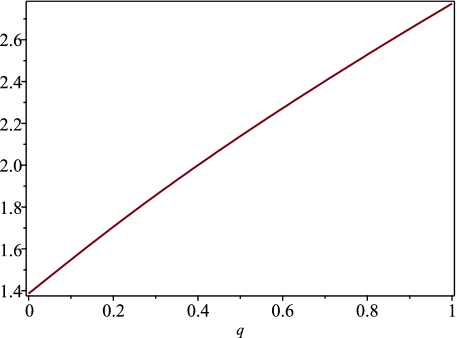
Figure 1: Plot of $2(1-q)F^{\prime}_{1}(0)$, showing the dependence of the constant term $\frac{2}{L}F^{\prime}_{1}(0)$ on $q$. We leave it as an exercise to show that, for $q\to 0$ (resp. $q\to 1$), the limit is $2\ln 2$ (resp. $4\ln 2$).

A question triggered by the observation that $\sum_{i\neq j}\textup{Cov}\,(X_{i,i}^{(n)},X_{j,j}^{(n)})=\mathcal{O}\left(\frac{1}{n}\right)$ is: How “close to being independent” are $\big{(}X_{i,i}^{(n)}\big{)}_{i\in\mathbb{N}}$ ? The following theorem provides a partial answer in that regard.

Theorem 2.2

The random variables $X_{i,i}^{(n)},i\in\mathbb{N}$ are asymptotically independent, in the sense that, for any $k\in\mathbb{N}$, any subset $I\subseteq\mathbb{N}$ of size $k$, and any $(x_{i})_{i\in I}\in\{0,1\}^{k}$ we have

$${\mathbb{P}}(X_{i,i}^{(n)}=x_{i},i\in I)-\prod_{i\in I}{\mathbb{P}}(X_{i,i}^{(n)}=x_{i})=\mathcal{O}\left(\frac{1}{n}\right),$$ (7)

with implied constant depending on $I$ only via $k$.

Remark 2.3

The random variables $\big{(}X_{i,i}^{(n)}\big{)}_{i\geq 1}$ are negatively correlated: For finite $I\subseteq\mathbb{N}$ we have

$${\mathbb{P}}(X_{i,i}^{(n)}=1,i\in I)\leq\prod_{i\in I}{\mathbb{P}}(X_{i,i}^{(n)}=1),$$

as can easily be deduced from the following theorem.
Theorem (McDiarmid (1992)): Let $V$ and $I$ be finite non-empty sets. Let $(Z_{v}:v\in V)$ be a family of independent random variables, each taking values in some set containing $I$; and for each $i\in I$, let $S_{i}=\{v\in V:Z_{v}=i\}$. Let $(\mathcal{F}_{i}:i\in I)$ be a family of collections of subsets of $V$ such that each collection is increasing (meaning that every superset of a set in $\mathcal{F}_{i}$ is also in $\mathcal{F}_{i}$) or each is decreasing (meaning that every subset of a set in $\mathcal{F}_{i}$ is also in $\mathcal{F}_{i}$). Then ${\mathbb{P}}\left(\bigcap_{i\in I}\{S_{i}\in\mathcal{F}_{i}\}\right)\leq\prod_{i\in I}{\mathbb{P}}\left(\{S_{i}\in\mathcal{F}_{i}\}\right)$.
We just have to choose $V:=\{1,\ldots,n\}$, and all $\mathcal{F}_{i}$ equal to $\mathcal{F}:=\{f\subseteq V:\exists k\in V:\{k,k+1\}\subseteq f\}$.

Cases like the following for $n=5$ and $i\neq j$,

$${\mathbb{P}}( X_{i,i}^{(5)}=1){\mathbb{P}}(X_{j,j}^{(5)}=1)-{\mathbb{P}}(X_{i,i}^{(5)}=X_{j,j}^{(5)}=1)$$

$$=\!P_{i}^{2}(4-2P_{i}-2P_{i}^{2}+P_{i}^{3})P_{j}^{2}(4-2P_{j}-2P_{j}^{2}+P_{j}^{3})-P_{i}^{2}P_{j}^{2}(6-2P_{i}-2P_{j})$$

$$=\!P_{i}^{2}P_{j}^{2}\left[(1\!-\!P_{i}\!-\!P_{j})(10\!+\!4P_{i}(1\!-\!P_{i})\!+\!4P_{j}(1\!-\!P_{j}))+P_{i}P_{j}(12\!+\!P_{i}(2\!-\!P_{i})P_{j}(2\!-\!P_{j})\!-\!2P_{i}^{2}\!-\!2P_{j}^{2})\right]\!>\!0$$

suggest that the inequality may be strict for $|I|\geq 2$. This is different for the array $\big{(}X_{i,j}^{(n)}\big{)}_{i,j\geq 1}$, where both strictly positive and strictly negative correlations can be observed: For $n=3$ and $i\neq j$,

$${\mathbb{P}}(X_{i,j}^{(3)}=X_{j,i}^{(3)}=1)-{\mathbb{P}}(X_{i,j}^{(3)}=1){\mathbb{P}}(X_{j,i}^{(3)}=1)=P_{i}P_{j}(P_{i}+P_{j})-(2P_{i}P_{j})^{2}=P_{i}P_{j}(P_{i}+P_{j}-4P_{i}P_{j})>0$$

holds for $P_{i},P_{j}$ small enough, and for different pairs $\big{(}(k_{i},m_{i})\big{)}_{i\in I}$, with $|I|\geq n$, we clearly have

$${\mathbb{P}}(X_{k_{i},m_{i}}^{(n)}=1,i\in I)=0<\prod_{i\in I}{\mathbb{P}}(X_{k_{i},m_{i}}^{(n)}=1).$$

3 Further conjectures and results for pairs of identical letters

3.1 Higher moments

The proof of Theorem 2.1 (see Lemma 4.8) shows that

$$\lim_{n\to\infty}(\textup{Var}\,X^{(n)}_{1}-\textup{Var}\,\xi^{(n)})=0,$$

where $\xi^{(n)}:=\sum_{i\geq 1}[[\xi_{i}^{(n)}\geq 1]]$ is a sum of independent random variables, with $\xi_{i}^{(n)}$ distributed as Poisson$(nP_{i}^{2})$. Note that ${\mathbb{P}}[X_{i,i}^{(n)}=0]\sim{\mathbb{P}}[\xi_{i}^{(n)}=0]$ and ${\mathbb{P}}[X_{i,i}^{(n)}=1]\sim{\mathbb{P}}[\xi_{i}^{(n)}\geq 1]$. This leads us to the following conjecture.

Conjecture 3.1

For any $k\in\mathbb{N}$ we have $\lim_{n\to\infty}(\mbox{$\mathbb{E}$}|X^{(n)}_{1}-\mbox{$\mathbb{E}$}X^{(n)}_{1}|^{k}-\mbox{$\mathbb{E}$}|\xi^{(n)}-\mbox{$\mathbb{E}$}\xi^{(n)}|^{k})=0$.

Theorem 3.2

If Conjecture 3.1 holds, the asymptotics of cumulants $\kappa_{m}^{(n)}$ of $X^{(n)}_{1}$ are given by

$$\kappa_{m}^{(n)}=m!\sum_{j=1}^{m}V^{(n)}_{j}\frac{(-1)^{j+1}}{j}[\theta^{m}](e^{\theta}-1)^{j},$$ (8)

where, using $L=\ln(1/q)$ again, asymptotics of $V^{(n)}_{j},\,j\geq 1$, are given by

$$V^{(n)}_{j}\sim\frac{\ln(np^{2})}{2L} +\frac{\gamma}{2L}+\frac{1}{2}+\frac{1}{2L}\sum_{k=2}^{j}(-1)^{k+1}{j\choose k}\ln k$$ (9)

$$+\frac{1}{2L}\sum_{\ell\neq 0}\left(\sum_{k=1}^{j}(-1)^{k}{j\choose k}k^{-\frac{\ell\chi}{2}}\right)\Gamma\left(\frac{\ell\chi}{2}\right)(np^{2})^{-\frac{\ell\chi}{2}}.$$

Proof.   We proceed as in Hitczenko and Louchard (2001) and Louchard and Prodinger (2006).

Let $S_{n}(\theta):=\ln(E(e^{\theta\xi^{(n)}}))=\sum_{m=1}^{\infty}\kappa_{m}^{(n)}\frac{\theta^{m}}{m!}$ be the cumulant generating function of $\xi^{(n)}$. Furthermore let $n_{2}:=np^{2}/q^{2}$, and observe $\mbox{$\mathbb{E}$}e^{\theta[[\xi_{i}^{(n)}\geq 1]]}=1+(e^{\theta}-1)(1-e^{-n_{2}q^{2i}})$. By independence of $\big{(}\xi_{i}^{(n)}\big{)}_{i\geq 1}$, we get

$$S_{n}(\theta) =\sum_{i=1}^{\infty}\ln\left[1+\left(e^{\theta}-1\right)\left(1-e^{-n_{2}q^{2i}}\right)\right]$$

$$=\sum_{j=1}^{\infty}\frac{(-1)^{j+1}}{j}(e^{\theta}-1)^{j}\left[\sum_{i=1}^{\infty}\left(1-e^{-n_{2}q^{2i}}\right)^{j}\right].$$

Now let

$$V^{(n)}_{j} :=\sum_{i=1}^{\infty}\left(1-e^{-n_{2}q^{2i}}\right)^{j}=\sum_{i=1}^{\infty}\left[\sum_{k=0}^{j}(-1)^{k}{j\choose k}e^{-kn_{2}q^{2i}}\right]$$

$$=\sum_{i=1}^{\infty}\left[\sum_{k=0}^{j}(-1)^{k}{j\choose k}e^{-kn_{2}q^{2i}}-\sum_{k=0}^{j}(-1)^{k}{j\choose k}\right]=\sum_{i=1}^{\infty}\left[\sum_{k=1}^{j}(-1)^{k+1}{j\choose k}\left(1-e^{-kn_{2}q^{2i}}\right)\right]$$

$$=\sum_{k=1}^{j}(-1)^{k+1}{j\choose k}\sum_{i=1}^{\infty}\left(1-e^{-kn_{2}q^{2i}}\right),$$

where the asymptotics of the inner sum can be obtained using $G(knp^{2})$ from Appendix A.1, leading to (9). Finally the cumulants $\kappa_{m}^{(n)}$ are found by extracting coefficients of $\theta^{m}$ from $S_{n}(\theta)$, and are given by finite linear combinations of the $(V^{(n)}_{j})_{j\geq 1}$, as stated in (8).  

Remark 3.3

Explicit expressions for (8) for small $m$ are

$$\kappa_{1}^{(n)}\!\!=V^{(n)}_{1},\quad\kappa_{2}^{(n)}\!=\!V^{(n)}_{1}\!-\!V^{(n)}_{2},\quad\kappa_{3}^{(n)}\!=\!V^{(n)}_{1}\!-\!3V^{(n)}_{2}\!+\!2V^{(n)}_{3},\quad\kappa_{4}^{(n)}\!=\!V^{(n)}_{1}\!-\!7V^{(n)}_{2}\!+\!12V^{(n)}_{3}\!-\!6V^{(n)}_{4}.$$

The fact that $\frac{1}{j!}(e^{x}-1)^{j}$ is the generating function for the Stirling numbers of the second kind, see e.g. (Flajolet and Sedgewick, 2009, p. 736), establishes that the sequence of (absolute values of) the coefficients, $(1,1,1,1,3,2,1,7,12,6,\ldots)$, is equal to OEIS sequence A028246 in Sloane .

The cumulants now allow for computation of moments: The mean of $X^{(n)}_{1}$ is given by

$$\mbox{$\mathbb{E}$}X^{(n)}_{1}\sim V^{(n)}_{1}.$$

This is identical to (Archibald et al., 2021, Thm. 2), see also (11). Our approach here is simple and general. Note that the mean does not rely on the state of Conjecture 3.1: the mean computation actually depends only on Lemma 4.3. Similarly, the variance of $X^{(n)}_{1}$ is given by

$$\textup{Var}\,X^{(n)}_{1}\sim V^{(n)}_{1}-V^{(n)}_{2}.$$

After some algebra, we verify that this is identical to Thm 2.1 .

3.2 Limiting distribution

A conjecture weaker than Conjecture 3.1 is

Conjecture 3.4

For any $t\in\mathbb{R}$ we have $\lim_{n\to\infty}[\mathbb{P}(X^{(n)}_{1}\leq t)-\mathbb{P}(\xi^{(n)}\leq t)]=0$.

Theorem 3.5

If Conjecture 3.4 holds, the asymptotic distribution $f(\eta)$ of $X^{(n)}_{1}$ is given by (10).

Set again $L=\ln(1/q)$ and $n_{2}=np^{2}/q^{2}$, set $i^{*}=\ln(n_{2})/(2L)$ (implying $q^{2i^{*}}=1/n_{2}$), define $\eta:=i-i^{*}$, and use ${\mathbb{P}}(\xi_{i}^{(n)}=0)=e^{-n_{2}q^{2i}}=\exp(-e^{-2L\eta})$. This leads to

$${\mathbb{P}}(\xi_{k}^{(n)}=0,k>i)=\exp\left(-\alpha e^{-2L\eta}\right),\mbox{ where }\alpha:=\frac{q^{2}}{1-q^{2}}.$$

As in Hitczenko and Louchard (2001) and Louchard et al. (2005), we proceed by defining

$$\Psi(\eta):=e^{-e^{-2L\eta}}\prod_{i=1}^{\infty}\left[1-e^{-e^{-2L(\eta-i)}}\right],$$

and observing that, as $n\to\infty$, we have

$${\mathbb{P}}(X^{(n)}_{1}=i^{*}+\eta)\sim \,f(\eta):=\sum_{v=0}^{\infty}\Psi(\eta-v+1)e^{-\alpha e^{-2L(\eta+1-v)}}\sum_{\overset{r_{1}<\cdots<r_{v}}{r_{j}\ \geq 2-v}}\prod_{i=1}^{v}\frac{1-e^{-e^{-2L(\eta+r_{i})}}}{e^{-e^{-2L(\eta+r_{i})}}},$$ (10)

$${\mathbb{P}}(X^{(n)}_{1}\leq i^{*}+\eta)\sim \,F(\eta):=\sum_{i=0}^{\infty}f(\eta-i).$$

$$f(\eta) \mbox{ depends only on }p.$$

A simulation with $p=1/4$ and $50000$ simulated words for each $n\in\{10000,11547,13333,15396\}$ is given in Figure 2. The fit is excellent.

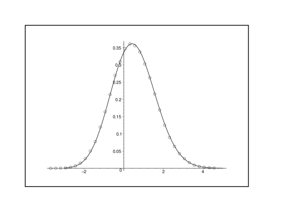
Figure 2: Comparison between $f(\eta)$ (line) and the simulation of $X^{(n)}_{1}$ (circles), $p=1/4$, number of simulated words $=50000$ for each $n\in\{10000,11547,13333,15396\}$.

A corresponding table of observed and theoretical non-periodic mean and variance in the equal pairs case (as well as another table for the unequal pairs case) is given below, all results rounded to 3 decimal places. We define $\bar{X}^{(n)}_{j}:=\frac{1}{N}\sum_{i=1}^{N}X_{j}^{(n),i}$ and $s_{j}^{2}(n):=\frac{1}{N-1}\sum_{i=1}^{N}(X_{j}^{(n),i}-\bar{X}^{(n)}_{j})^{2}$ the sample mean and unbiased sample variance of a sample $(X_{j}^{(n),i})_{i=1}^{N}$. See Theorem 3.7 for asymptotics of $\mbox{$\mathbb{E}$}X^{(n)}_{1}$ and $\mbox{$\mathbb{E}$}X^{(n)}_{3}$. Both simulations use $p=1/4$. The sample size $N$ for each row in the left table is $50000$, and in the right table it is $200000$, see also Figure 3.

$$n$$

   

Remark 3.6

Here we briefly sketch, how we obtained the graph of $f$ in Figure 2, where $p=1/4$. As before, we use random variables $\xi_{i}^{(n)}$ distributed Poisson$(np^{2}q^{2(i-1)})$, but now there is such a random variable for each $i\in\mathbb{Z}$ and each real $n>0$. For fixed such $n$ the random variables $\big{(}\xi^{(n)}_{i}\big{)}_{i\in\mathbb{Z}}$ are assumed independent, and also the definition $\xi^{(n)}:=\sum_{i\geq 1}\xi^{(n)}_{i}$ is used for real $n>0$. We use $i^{*}=i^{*}(n)=\ln(np^{2}/q^{2})/(2L)$ again. For any $n$ satisfying $i^{*}+\eta\in\mathbb{Z}$, we have

$$f(\eta) =\lim_{k\to\infty}{\mathbb{P}}\Big{(}\xi^{(nq^{-2k})}-k=i^{*}+\eta\Big{)}={\mathbb{P}}\Big{(}\sum_{i\geq 1}[[\xi_{i}^{(n)}\geq 1]]+\sum_{j\geq 0}([[\xi_{-j}^{(n)}\geq 1]]-1)=i^{*}+\eta\Big{)}$$

$$={\mathbb{P}}\Big{(}\sum_{i\geq 1}[[\xi_{i}^{(\nu)}\geq 1]]+\sum_{j\geq 0}([[\xi_{-j}^{(\nu)}\geq 1]]-1)=0\Big{)},$$

where for $n=\nu=\nu(\eta):=q^{2(1-\eta)}/p^{2}$ we have $i^{*}+\eta=0$, and $\xi^{(\nu)}_{i}\sim$ Poisson$\big{(}q^{2(i-\eta)}\big{)}$. We want a good approximation of $f(\eta)$ only for $\eta\in[-3,5]$. For such $\eta$ we have

$${\mathbb{P}}\Big{(}\sum_{i>30}[[\xi_{i}^{(\nu)}\geq 1]]>0\Big{)}=1-\prod_{i>30}e^{-q^{2i-2\eta}}\leq 1-\prod_{i>30}e^{-q^{2i-10}}=1-\exp\left(-\frac{q^{52}}{1-q^{2}}\right)\approx 7.28\cdot 10^{-7}.$$

and

$${\mathbb{P}}\Big{(}\sum_{j>7}([[\xi_{-j}^{(\nu)}\geq 1]]-1)<0\Big{)}=1-\prod_{j>7}\Big{(}1-e^{-q^{-2j-2\eta}}\Big{)}\leq\sum_{j>7}e^{-q^{6-2j}}\approx e^{-q^{-10}}\approx 1.94\cdot 10^{-8}.$$

So, up to an error smaller than $10^{-6}$, $f(\eta)$ is given by

$${\mathbb{P}}\Big{(}\sum_{i=1}^{30}[[\xi_{i}^{(\nu)}\geq 1]]+\sum_{j=0}^{7}([[\xi_{-j}^{(\nu)}\geq 1]]-1)=0\Big{)} ={\mathbb{P}}\Big{(}\sum_{i=-7}^{30}[[\xi_{i}^{(\nu)}\geq 1]]\!=\!8\Big{)}$$

$$=[z^{8}]\!\prod_{i=-7}^{30}\!\bigg{(}1+(z-1)\big{(}1-e^{-q^{2i-2\eta}}\big{)}\bigg{)},$$

where, for each fixed $\eta$, the latter coefficient can easily be computed using Maple.

Theorem 3.7

(see (Archibald et al., 2021, Thm. 2, Thm. 3)) Let $L:=\ln(1/q)$ and $\chi:=2\pi\mathbf{i}/L$. Then, as $n\to\infty$, the expectations of $X^{(n)}_{i}$, $i\in\{1,3\}$, satisfy

$$\mbox{$\mathbb{E}$}X^{(n)}_{1} \sim\frac{\ln(np^{2})}{2L}+\frac{1}{2}+\frac{\gamma}{2L}-\frac{1}{2L}\sum_{\ell\neq 0}\Gamma\Big{(}\frac{\ell\chi}{2}\Big{)}(np^{2})^{-\ell\chi/2},$$ (11)

$$\mbox{$\mathbb{E}$}X^{(n)}_{3} \sim\frac{\ln^{2}(np^{2})}{2L^{2}}+\Big{[}\frac{\gamma}{L^{2}}+\frac{1}{2L}\Big{]}\ln(np^{2})+\frac{\pi^{2}+6\gamma^{2}}{12L^{2}}+\frac{\gamma}{2L}-\frac{1}{12}$$

$$~{}~{}~{}~{}~{}~{}~{}~{}~{}~{}~{}~{}~{}~{}~{}-\frac{\ln(np^{2})}{L^{2}}\sum_{\ell\neq 0}\Gamma(\ell\chi)(np^{2})^{-\ell\chi}$$ (12)

$$~{}~{}~{}~{}~{}~{}~{}~{}~{}~{}~{}~{}~{}~{}~{}+\frac{1}{L^{2}}\sum_{\ell\neq 0}\Gamma^{\prime}(\ell\chi)(np^{2})^{-\ell\chi}-\frac{1}{2L}\sum_{\ell\neq 0}(-1)^{\ell}\Gamma\Big{(}\frac{\ell\chi}{2}\Big{)}(np^{2})^{-\ell\chi/2}.$$

4 The probability of avoiding certain pairs via Markov chains.

4.1 Two pairs $(i,i)$ and $(r,r)$ of identical letters

The proofs of the theorems rest upon calculation of probabilities of avoiding certain pairs, which we will be doing by employing Markov chains. To illustrate that approach, we consider in greater detail the case of avoiding two fixed pairs $(i,i)$ and $(r,r)$, where $i\neq r$, in a sequence of length $n$. No distinction of letters different from $i,r$ is necessary, so for our Markov chain we can use a finite state space $S:=\{e,i,r,\Delta\}$, where $e:=\mathbb{N}\setminus\{i,r\}$ stands for “everything else”, i.e., the set $\mathbb{N}\setminus\{i,r\}$ is lumped together, and $\Delta$ denotes an additional cemetery state. The corresponding state diagram is

From any realization $(z_{k})_{k\geq 1}$ of the i.i.d. sequence $(Z_{k})_{k\geq 1}$ we obtain a trajectory $(y_{k})_{k\geq 0}$ of this finite state Markov chain via

$$(y_{0},y_{1},y_{2},\ldots)=(e,\phi(z_{1}),\phi(z_{2}),\phi(z_{3}),\ldots),$$

where $\phi(z_{k}):=\Delta$ if for some $j<k$ we have $(z_{j},z_{j+1})\in\{(i,i),(r,r)\}$, and otherwise

$$\phi(z_{k})=\begin{cases}z_{k},&z_{k}\in\{i,r\}\\ e,&\textup{else}.\end{cases}$$

Example: If $n=8,i=1,r=2$ then the sequences $(1,2,3,1,2,3,4,5)$ and $(3,2,1,1,4,3,2,2)$ yield trajectories $(e,1,2,e,1,2,e,e,e)$ and $(e,e,2,1,\Delta,\Delta,\Delta,\Delta,\Delta)$.

Those trajectories $(y_{k})_{k=0}^{n}$ satisfying $y_{n}\neq\Delta$ are in correspondence to sequences $(z_{k})_{k=1}^{n}$ that avoid the pairs $(i,i)$ and $(r,r)$. Using the transition matrix

$$\Pi:=\begin{bmatrix}P_{e}&P_{i}&P_{r}&0\\ P_{e}&0&P_{r}&P_{i}\\ P_{e}&P_{i}&0&P_{r}\\ 0&0&0&1\end{bmatrix},$$

where $P_{e}:=1-P_{i}-P_{r}$, the sought probability is $[1,0,0,0]\,\Pi^{n}\,[1,1,1,0]^{t}$, respectively, using the restriction $\bar{\Pi}$ of $\Pi$ to $\{e,i,r\}$, i.e.,

$$\bar{\Pi}:=\begin{bmatrix}P_{e}&P_{i}&P_{r}\\ P_{e}&0&P_{r}\\ P_{e}&P_{i}&0\end{bmatrix},$$

and initial probability $\pi(\cdot):=[1,0,0]$ and column vector of all ones $\mathds{1}$, that probability is

$${\mathbb{P}}(X_{i,i}^{(n)}=X_{r,r}^{(n)}=0)=\pi\,\bar{\Pi}^{n}\,\mathds{1}.$$

A bound on such probability will now be derived in the following more general context.

We fix a finite non-empty set of forbidden pairs

$$\mathcal{I}:=\{(k_{i},m_{i}):i\in I\}$$

of size $|I|$, and let

$$J:=\bigcup_{i\in I}\{k_{i},m_{i}\}=\{j_{1},\ldots,j_{|J|}\},$$

where $j_{1}<\ldots<j_{|J|}$. Moreover we fix $0<\delta\leq 1/2$ and let

$$\mathcal{D}^{J}_{\delta}:=\{\mathbf{x}\in\mathbb{R}^{|J|}:x_{j}\geq 0\mbox{ for }j\in J,\,\sum_{j\in J}x_{j}\leq 1-\delta\}.$$

Lemma 4.1

Let $\varepsilon:=\sum_{i\in I}P_{k_{i}}P_{m_{i}}$. Then

$${\mathbb{P}}(X_{k_{i},m_{i}}^{(n)}=0,i\in I)\leq\delta^{-1/2}e^{-\varepsilon n/2}$$ (13)

holds for $(P_{j})_{j\in J}\in\mathcal{D}^{J}_{\delta}$. Furthermore, there are functions $\lambda_{1},C_{1}$ and $\Phi_{n},n\geq 1$, depending on $P_{j},j\in J$, that are $C^{\infty}$ and positive on an open set $\mathcal{F}$ satisfying $\mathcal{D}^{J}_{\delta}\subseteq\mathcal{F}$, such that

$${\mathbb{P}}(X_{k_{i},m_{i}}^{(n)}=0,i\in I)=C_{1}\lambda_{1}^{n}\Phi_{n}.$$ (14)

Remark 4.2

At several places we take the liberty to regard $(P_{j})_{j\geq 1}$ as variables (which is slight abuse of notation), to the effect, that several results in this section hold more generally also for strings of random variables with a distribution different from the geometric. The reader must be prepared to see expressions involving $\lim_{P_{j}\to 0}$, $\frac{\partial}{\partial P_{j}}$, and functions of $(P_{j})_{j\in J}$ being $C^{\infty}$ in some domain, etc. all the time. In particular, we allow $(P_{j})_{j\in J}$ to vary within the set $\mathcal{D}^{J}_{\delta}$ above, which is a proper subset of the unit simplex of dimension $|J|$, because some of our results require $P_{e}$ to be bounded away from zero.

Proof of Lemma 4.1. Assume $P_{j}>0$ for $j\in J$, as well as $P_{e}:=1-\sum_{j\in J}P_{j}\geq\delta$. Note that $\varepsilon\leq\sum_{j,\ell\in J}P_{j}P_{\ell}=(1-P_{e})^{2}\leq(1-\delta)^{2}<1-\delta$. Define the matrix $\bar{\Pi}$ with rows and columns indexed by the set $J\cup\{e\}$ (which we assume ordered, starting with $e$ and followed by the elements of $J$ in ascending order) via

$$\bar{\Pi}_{k,m}:=\begin{cases}0,&(k,m)\in\mathcal{I},\\ P_{m},&\textup{else.}\end{cases}$$

We define a row vector $\mathbf{w}:=[\ \sqrt{P_{e}},\sqrt{P_{j_{1}}},\ldots,\sqrt{P_{j_{|J|}}}\ ]$, satisfying $\|\mathbf{w}\|_{2}=1$, and a diagonal matrix $S:=\textup{Diag}(\mathbf{w})$, and the matrix

$$\hat{\Pi}:=S\bar{\Pi}S^{-1}=S\left[\mathds{1}\mathds{1}^{t}-\sum_{i\in I}\mathbf{e}_{k_{i}}\mathbf{e}_{m_{i}}^{t}\right]S,$$

where the column vectors $\mathbf{e}_{j},j\in J\cup\{e\}$, denote the standard unit vectors in $\mathbb{R}^{|J|+1}$, and observe, using the Frobenius norm $\|\hat{\Pi}\|_{F}=\sqrt{\sum_{k,m\in J\cup\{e\}}\hat{\Pi}_{k,m}^{2}}=\sqrt{1-\sum_{i\in I}P_{k_{i}}P_{m_{i}}}$, and $\pi=(\mathbf{e}_{e})^{t}$,

$$\mathbb{P}(X_{k_{i},m_{i}}^{(n)}=0,i\in I) =\pi\bar{\Pi}^{n}\mathds{1}=\mathbf{w}\hat{\Pi}^{n-1}\mathbf{w}^{t}$$

$$\leq\|\mathbf{w}\|_{2}^{2}\|\hat{\Pi}\|_{2}^{n-1}\leq\|\hat{\Pi}\|_{F}^{n-1}=(1-\varepsilon)^{(n-1)/2}\leq\delta^{-1/2}(1-\varepsilon)^{n/2}\leq\delta^{-1/2}e^{-\varepsilon n/2}.$$

Observe that $\bar{\Pi}$ is non-negative and primitive, therefore, by the Perron-Frobenius Theorem (see Seneta (1981)), there is a unique positive eigenvalue $\lambda_{1}$, that is strictly larger in modulus than any other eigenvalue, and corresponding strictly positive left and right eigenvectors $\mathbf{u}$ and $\mathbf{v}$, such that $\bar{\Pi}^{n}=\frac{\lambda_{1}^{n}}{\mathbf{u}\mathbf{v}}\mathbf{v}\mathbf{u}+\mathcal{O}(n^{|J|}|\lambda_{2}|^{n})$ element-wise, where $\lambda_{2}$ is an eigenvalue of second largest modulus. This leads to

$$\mathbb{P}(X_{k_{i},m_{i}}^{(n)}=0,i\in I)=\frac{(\pi\mathbf{v})(\mathbf{u}\mathds{1})}{\mathbf{u}\mathbf{v}}\lambda_{1}^{n}+\mathcal{O}(n^{|J|}|\lambda_{2}|^{n}).$$

By setting one or more of $(P_{j})_{j\in J}$ to zero, one or more of the non-dominant eigenvalues $(\lambda_{k})_{k\geq 2}$ become zero, but there is a non-negative primitive submatrix constructed from the non-zero columns (and corresponding rows) of $\bar{\Pi}$, guaranteeing a unique positive eigenvalue larger in modulus than all other eigenvalues. As the row and column corresponding to state $e$ will always be part of that submatrix, the first components $u_{e}$ and $v_{e}$ of $\mathbf{u}$ and of $\mathbf{v}$ will be positive. By continuity, these properties also hold in a neighbourhood of such $(P_{j})_{j\in J}$, which yields $\lambda_{1}$ being $C^{\infty}$ in some open superset $\bar{\mathcal{F}}$ of $\mathcal{D}^{J}_{\delta}$, by the implicit function theorem, using the facts that the characteristic polynomial $p(\lambda)$ of $\bar{\Pi}$, considered as a function of $(\lambda,(P_{j})_{j\in J})$, is $C^{\infty}$, and the derivative of $p(\lambda)$ evaluated in a simple zero $\lambda_{1}$ is non-zero. On the set $\bar{\mathcal{F}}$, the components of $\frac{1}{u_{e}}\mathbf{u}$ and $\frac{1}{v_{e}}\mathbf{v}$ are $C^{\infty}$ functions of $(P_{j})_{j\in J}$ as well.

We let $C_{1}:=\frac{(\pi\mathbf{v})(\mathbf{u}\mathds{1})}{\mathbf{u}\mathbf{v}}$ and $\Phi_{n}:=\frac{1}{C_{1}}\lambda_{1}^{-n}\mathbb{P}(X_{k_{i},m_{i}}^{(n)}=0,i\in I)$. Those are positive $C^{\infty}$ functions of $(P_{j})_{j\in J}$ on an open set $\mathcal{F}$, satisfying $\mathcal{D}^{J}_{\delta}\subseteq\mathcal{F}\subseteq\bar{\mathcal{F}}$, the further restriction made necessary by the need to avoid $\mathbf{u}\mathbf{v}\leq 0$, which may occur for $(P_{j})_{j\in J}$ outside $\mathcal{D}^{J}_{\delta}$. Note that primitivity of $\bar{\Pi}$ may cease to hold when $P_{e}=0$. Moreover note that $|\lambda_{2}|$ is continuous on $\mathcal{D}_{\delta}^{J}$, but need not be differentiable on that set.  
The bound (13) fits our needs when $\varepsilon$ is large. Equation (14) is useful in the case of small $\varepsilon$, if asymptotics of $\lambda_{1},C_{1}$ and $\Phi_{n}$ are known. In order to derive such asymptotics, we let $\bar{\bar{\Pi}}$ be the matrix obtained from $\bar{\Pi}$ by deleting row and column corresponding to state $e$. Left and right eigenvectors $\mathbf{u}=[1,\beta]$ and $\mathbf{v}=[1/P_{e},\mu^{t}]^{t}$, with row vector $\beta=(\beta_{j})_{j\in J}$ and column vector $\mu=(\mu_{j})_{j\in J}$, corresponding to the dominant eigenvalue $\lambda_{1}$ of $\bar{\Pi}$, lead to equations

$$\lambda_{1} =P_{e}(1+\sum_{j\in J}\beta_{j})=P_{e}(1+\sum_{j\in J}P_{j}\mu_{j}),$$ (15)

$$\beta =\frac{1}{\lambda_{1}}\left[\beta\bar{\bar{\Pi}}+\bar{\mathbf{p}}\right],$$ (16)

$$\mu =\frac{1}{\lambda_{1}}\left[\bar{\bar{\Pi}}\mu+\mathds{1}\right],$$ (17)

with row vector $\bar{\mathbf{p}}=(P_{j})_{j\in J}$, and with ascending order of indices in $\beta,\mu,\bar{\mathbf{p}}$. We keep denoting the column vector of all ones of appropriate dimension by $\mathds{1}$, and express $C_{1}$ in terms of $\beta$ and $\mu$ as follows:

$$C_{1}=\frac{(\pi\mathbf{v})(\mathbf{u}\mathds{1})}{\mathbf{u}\mathbf{v}}=\frac{\frac{1}{P_{e}}(1+\sum_{j\in J}\beta_{j})}{\frac{1}{P_{e}}+\sum_{j\in J}\beta_{j}\mu_{j}}=\frac{1+\beta\mathds{1}}{1+P_{e}\beta\mu}.$$ (18)

Asymptotics up to any fixed order $K$ of $\lambda_{1},\beta,\mu$ are conveniently computed via fixed point iteration as described by the following algorithm:

Algorithm 1 Calculate asymptotics of $\lambda_{1},\beta,\mu$ up to fixed order.

0:  $K\geq 0,k=0,\bar{\bar{\Pi}},\bar{\mathbf{p}},\lambda=1,\bar{\beta}=[0,\ldots,0],\bar{\mu}=[1,\ldots,1]^{t}$

  while $k<K$ do

     $\bar{\beta}\leftarrow\frac{1}{\lambda}\big{[}\bar{\beta}\bar{\bar{\Pi}}+\bar{\mathbf{p}}\big{]}$

     $\lambda\leftarrow P_{e}[1+\bar{\beta}\mathds{1}]$

     $\bar{\mu}\leftarrow\frac{1}{\lambda}\big{[}\bar{\bar{\Pi}}\bar{\mu}+\mathds{1}\big{]}$

     $k\leftarrow k+1$

  end while

  return  $\lambda,\bar{\beta},\bar{\mu}$

The output $\lambda,\bar{\beta},\bar{\mu}$ of the algorithm then satisfies $\lambda_{1}=\lambda+\mathcal{O}^{*}_{K+1}$, $\beta=\bar{\beta}+\mathcal{O}^{*}_{K+1}$, $\mu=\bar{\mu}+\mathcal{O}^{*}_{K+1}$. Here and in the following the notation $\mathcal{O}_{k}^{*}$ always refers to the variables $(P_{j})_{j\in J}$, but not to $P_{e}$. So, for instance, $\mathcal{O}_{4}^{*}$ is the same as $\mathcal{O}(\gamma^{4})$, where $\gamma=\sum_{j\in J}P_{j}$.

A few words on justification of the algorithm: First note, that nothing changes if the line $\lambda\leftarrow P_{e}[1+\bar{\beta}\mathds{1}]$ is replaced by $\lambda\leftarrow P_{e}[1+\bar{\mathbf{p}}\bar{\mu}]$. This is seen to hold for $k=0$, where $\bar{\beta}=\bar{\mathbf{p}}$ has already been updated, but $\bar{\mu}=\mathds{1}$ has not, and for $k>0$ by a simple induction step. We can thus see Algorithm 1 as a combination of two algorithms, one of them only updating the pair $(\bar{\beta},\lambda)$, the other only updating the pair $(\lambda,\bar{\mu})$, with those algorithms having identical updates of $\lambda$. Let us concentrate on the latter algorithm. Denote $x=(\lambda,\bar{\mu})$ and let $\mathbb{0}$ be the zero vector of appropriate dimension. Observe that the function $F(x,\bar{\mathbf{p}})=\left[\begin{smallmatrix}\lambda-P_{e}[1+\bar{\mathbf{p}}\bar{\mu}]\\ \bar{\mu}-\frac{1}{\lambda}\big{[}\bar{\bar{\Pi}}\bar{\mu}+\mathds{1}\big{]}\end{smallmatrix}\right]$ is $C^{\infty}$ in a neighbourhood of $(x_{0},\bar{\mathbf{p}}_{0}):=(1,\mathds{1},\mathbb{0})$, with $F(x_{0},\bar{\mathbf{p}}_{0})=\mathbb{0}$. Now the Jacobian $JF(x_{0},\bar{\mathbf{p}}_{0})$ is nonsingular, so there is a unique $C^{\infty}$ function $x(\bar{\mathbf{p}})=(\lambda_{1}(\bar{\mathbf{p}}),\mu(\bar{\mathbf{p}}))$ defined in some neighbourhood $\mathcal{V}$ of $\bar{\mathbf{p}}=\mathbb{0}$, satisfying $x(\mathbb{0})=x_{0}$ and $F(x(\bar{\mathbf{p}}),\bar{\mathbf{p}})=\mathbb{0}$ for $\bar{\mathbf{p}}\in\mathcal{V}$, by the implicit function theorem. Denoting iterates by

$\lambda^{k+1}=f(\bar{\mu}^{k})=P_{e}[1+\bar{\mathbf{p}}\bar{\mu}^{k}]$ and  $\bar{\mu}^{k+1}=\frac{1}{\lambda^{k+1}}g(\bar{\mu}^{k})=\frac{1}{\lambda^{k+1}}[\bar{\bar{\Pi}}\bar{\mu}^{k}+\mathds{1}]$,

with $\lambda^{0}=1$ and $\bar{\mu}^{0}=\mathds{1}$, we can easily check $|\lambda_{1}(\bar{\mathbf{p}})-\lambda^{0}|=\mathcal{O}_{1}^{*}$ and $\|\mu_{1}(\bar{\mathbf{p}})-\bar{\mu}^{0}\|=\mathcal{O}_{1}^{*}$, for $\bar{\mathbf{p}}\in\mathcal{V}$.
Assume now that we have already shown $|\lambda_{1}(\bar{\mathbf{p}})-\lambda^{k-1}|=\mathcal{O}_{k}^{*}$ and $\|\mu(\bar{\mathbf{p}})-\bar{\mu}^{k-1}\|=\mathcal{O}_{k}^{*}$. Then we have $|\lambda_{1}(\bar{\mathbf{p}})-\lambda^{k}|=|f(\mu(\bar{\mathbf{p}}))-f(\mu^{k-1})|=|P_{e}\bar{\mathbf{p}}(\mu(\bar{\mathbf{p}})-\mu^{k-1})|=\mathcal{O}_{1}^{*}\|\mu(\bar{\mathbf{p}})-\bar{\mu}^{k-1}\|=\mathcal{O}_{k+1}^{*}$, and $\|\mu(\bar{\mathbf{p}})-\bar{\mu}^{k}\|=\|\frac{1}{\lambda_{1}}g(\mu(\bar{\mathbf{p}}))-\frac{1}{\lambda^{k}}g(\bar{\mu}^{k-1})\|\leq\|(\frac{1}{\lambda_{1}}-\frac{1}{\lambda^{k}})g(\mu(\bar{\mathbf{p}}))\|+\|\frac{1}{\lambda^{k}}(g(\mu(\bar{\mathbf{p}}))-g(\bar{\mu}^{k-1}))\|=\mathcal{O}_{k+1}^{*}$, because $(\frac{1}{\lambda_{1}}\!-\!\frac{1}{\lambda^{k}})g(\mu(\bar{\mathbf{p}}))\!=\!\frac{\lambda^{k}-\lambda_{1}}{\lambda^{k}}\mu(\bar{\mathbf{p}})\!=\!\mathcal{O}_{k+1}^{*}$, and $\frac{1}{\lambda^{k}}(g(\mu(\bar{\mathbf{p}}))\!-\!g(\bar{\mu}^{k-1}))\!=\!\frac{1}{\lambda^{k}}\bar{\bar{\Pi}}(\mu(\bar{\mathbf{p}})\!-\!\bar{\mu}^{k-1})\!=\!\mathcal{O}_{k+1}^{*}$.

The next lemma provides asymptotics of probabilities in the case of a single avoided pair.

Lemma 4.3

The probabilities of avoiding the pair $(i,i)$, resp. $(i,r)$ for $i\neq r$, in a sequence of length $n$ satisfy

$${\mathbb{P}}(X_{i,i}^{(n)}=0) =e^{-nP_{i}^{2}}+\mathcal{O}\big{(}\sqrt{n}P_{i}^{2}e^{-\frac{2-\delta}{4}nP_{i}^{2}}\big{)},$$ (19)

$${\mathbb{P}}(X_{i,r}^{(n)}=0) =e^{-nP_{i}P_{r}}+\mathcal{O}\big{(}P_{i}P_{r}e^{-\frac{2-\delta}{4}nP_{i}P_{r}}\big{)},$$ (20)

as $n\to\infty$, uniformly for $P_{i}\in\mathcal{D}^{\{i\}}_{\delta}$, resp. for $(P_{i},P_{r})\in\mathcal{D}^{\{i,r\}}_{\delta}$.

Proof.   We first consider the forbidden pair $(i,i)$. The matrix $\bar{\Pi}$, its characteristic polynomial $p$, and asymptotics of $\lambda_{1}$ and $C_{1}$ are given by

$$\bar{\Pi}=\begin{bmatrix}P_{e}&P_{i}\\ P_{e}&0\\ \end{bmatrix},\qquad\begin{aligned} p(\lambda)&=\lambda^{2}-(1-P_{i})\lambda-P_{i}P_{e},\\ \lambda_{1}&=1-P_{i}^{2}+P_{i}^{3}-2P_{i}^{4}+\mathcal{O}_{5}^{*},\\ C_{1}&=1+P_{i}^{2}-2P_{i}^{3}+6P_{i}^{4}+\mathcal{O}_{5}^{*},\end{aligned}$$

where we used Algorithm 1 (with $K=4$) and (18).

Following a suggestion by Salvy , we can easily derive $\lambda_{1}$ from $p(\lambda)$, after replacing $P_{e}$ by $1-P_{i}$. We add an extra variable $v$, carrying the weight of the $P_{.}:\tilde{P}_{.}:=vP_{.}$. We have the local expansion of the solution at $0$ by using the Maple package gfun (see Salvy and Zimmermann (1994)):

$$sol:=\mbox{gfun}[\mbox{algeqtoseries}](p(\lambda),v,\lambda,pr),$$

where $pr$ denotes the precision of the expansion into $v$. We obtain the solutions as $sol[1],sol[2]$ and we keep the solution close to $1$.

Denoting $\pi\bar{\Pi}^{n}\mathds{1}=C_{1}\lambda_{1}^{n}+C_{2}\lambda_{2}^{n}$, with $\lambda_{2}$ the non-dominant eigenvalue of $\bar{\Pi}$, we have $C_{1}\lambda_{1}^{0}+C_{2}\lambda_{2}^{0}=1$, and therefore $C_{2}=-P_{i}^{2}+2P_{i}^{3}-6P_{i}^{4}+\mathcal{O}_{5}^{*}$, which leads to $\Phi_{n}=1+\frac{C_{2}}{C_{1}}\big{(}\frac{\lambda_{2}}{\lambda_{1}}\big{)}^{n}=1+\mathcal{O}(P_{i}^{2})$, uniformly in $n$. This is used in (14), together with $C_{1}=1+\mathcal{O}(P_{i}^{2})$ and

$$\lambda_{1}^{n}=e^{n\ln\lambda_{1}}=e^{n(-P_{i}^{2}+P_{i}^{3}+\mathcal{O}(P_{i}^{4}))}=e^{-nP_{i}^{2}}(1+\mathcal{O}(nP_{i}^{3}))$$

leading to ${\mathbb{P}}(X_{i,i}^{(n)}=0)=\left[1+\mathcal{O}(P_{i}^{2})+\mathcal{O}(nP_{i}^{3})\right]e^{-nP_{i}^{2}}$, for $nP_{i}^{3}=\mathcal{O}(1)$, resp. for $nP_{i}^{2}=\mathcal{O}(n^{1/3})$. Note that for fixed $\alpha,\beta\!>\!0$ the function $x^{\alpha}e^{-\beta x}$ is bounded for $x>0$, implying

$$nP_{i}^{3}e^{-nP_{i}^{2}}=\sqrt{n}P_{i}^{2}(nP_{i}^{2})^{1/2}e^{-\frac{2+\delta}{4}nP_{i}^{2}}e^{-\frac{2-\delta}{4}nP_{i}^{2}}=\mathcal{O}\Big{(}\sqrt{n}P_{i}^{2}e^{-\frac{2-\delta}{4}nP_{i}^{2}}\Big{)}.$$

Moreover also $P_{i}^{2}e^{-nP_{i}^{2}}=\mathcal{O}\Big{(}\sqrt{n}P_{i}^{2}e^{-\frac{2-\delta}{4}nP_{i}^{2}}\Big{)}$ holds, and (13) can be built in by observing that $nP_{i}^{2}=\Omega(n^{1/3})$ implies $\delta^{-1/2}e^{-\frac{n}{2}P_{i}^{2}}=\mathcal{O}\Big{(}\sqrt{n}P_{i}^{2}e^{-\frac{2-\delta}{4}nP_{i}^{2}}\Big{)}$. We have thus obtained (19).

We now consider the forbidden pair $(i,r)$ with $i\neq r$. The matrix $\bar{\Pi}$, its characteristic polynomial $p$, and asymptotics of $\lambda_{1}$ and $C_{1}$ are given by

$$\bar{\Pi}=\begin{bmatrix}P_{e}&P_{i}&P_{r}\\ P_{e}&P_{i}&0\\ P_{e}&P_{i}&P_{r}\\ \end{bmatrix},\qquad\begin{aligned} p(\lambda)&=\lambda^{3}-\lambda^{2}+P_{i}P_{r}\lambda,\\ \lambda_{1}&=1-P_{i}P_{r}-P_{i}^{2}P_{r}^{2}-2P_{i}^{3}P_{r}^{3}+\mathcal{O}_{8}^{*},\\ C_{1}&=1+P_{i}P_{r}+3P_{i}^{2}P_{r}^{2}+10P_{i}^{3}P_{r}^{3}+\mathcal{O}_{8}^{*}.\end{aligned}$$

Clearly, $\lambda_{1}$, and therefore also $C_{1}$ and $\Phi_{n}$, are $C^{\infty}$ functions of the coefficient $P_{i}P_{r}$ of the characteristic polynomial $p$, meaning that the error term $\mathcal{O}_{8}^{*}$ is in fact $\mathcal{O}(P_{i}^{4}P_{r}^{4})$. Sufficiently accurate for our purposes are the asymptotics $\lambda_{1}=1-P_{i}P_{r}+\mathcal{O}(P_{i}^{2}P_{r}^{2})$ and $C_{1}=1+\mathcal{O}(P_{i}P_{r})$.

One of the eigenvalues is $0$, therefore a representation $\pi\bar{\Pi}^{n}\mathds{1}=C_{1}\lambda_{1}^{n}+C_{2}\lambda_{2}^{n}$ as before also holds in this case, with $C_{2}=\mathcal{O}(P_{i}P_{r})$, and $\Phi_{n}=1+\frac{C_{2}}{C_{1}}\big{(}\frac{\lambda_{2}}{\lambda_{1}}\big{)}^{n}=1+\mathcal{O}(P_{i}P_{r})$, uniformly in $n$. All this, together with $\lambda_{1}^{n}=e^{-nP_{i}P_{r}}(1+\mathcal{O}(nP_{i}^{2}P_{r}^{2}))$, leads to (20) via (14), taking care of error terms as above.  
The next corollary follows easily from equations (13), (19) and (20).

Corollary 4.4

The variances of $X_{i,i}^{(n)}$ and $X_{i,r}^{(n)}$ for $i\neq r$ satisfy

$$\textup{Var}\,X_{i,i}^{(n)} =e^{-nP_{i}^{2}}-e^{-2nP_{i}^{2}}+\mathcal{O}\big{(}\sqrt{n}P_{i}^{2}e^{-\frac{2-\delta}{4}nP_{i}^{2}}\big{)},$$ (21)

$$\textup{Var}\,X_{i,r}^{(n)} =e^{-nP_{i}P_{r}}-e^{-2nP_{i}P_{r}}+\mathcal{O}\big{(}P_{i}P_{r}e^{-\frac{2-\delta}{4}nP_{i}P_{r}}\big{)},$$ (22)

as $n\to\infty$, uniformly for $P_{i}\in\mathcal{D}^{\{i\}}_{\delta}$, resp. for $(P_{i},P_{r})\in\mathcal{D}^{\{i,r\}}_{\delta}$.

In order to obtain asymptotics for the covariance

$$\textup{Cov}\,(X_{i,i}^{(n)},X_{r,r}^{(n)}) ={\mathbb{P}}(X_{i,i}^{(n)}\!=\!X_{r,r}^{(n)}\!=\!1)-{\mathbb{P}}(X_{i,i}^{(n)}\!=\!1){\mathbb{P}}(X_{r,r}^{(n)}\!=\!1)$$

$$={\mathbb{P}}(X_{i,i}^{(n)}\!=\!X_{r,r}^{(n)}\!=\!0)-{\mathbb{P}}(X_{i,i}^{(n)}\!=\!0){\mathbb{P}}(X_{r,r}^{(n)}\!=\!0),$$

we need the following result.

Lemma 4.5

Let $A\in\mathbb{R}^{k\times k}$, with $k\geq 2$, have spectral radius $\rho(A)\leq 1$ and Frobenius norm $\|A\|_{F}=C^{\prime}$. Then, with $C:=\max(C^{\prime},k)$ and $C^{\prime\prime}:=2C^{k-1}$, we have

$$\|A^{n}\|_{F}\leq C^{\prime\prime}n^{k-1}.$$

Proof.   We use Schur decomposition, according to which there is a unitary matrix $Q$ such that $\bar{A}:=QAQ^{-1}$ is upper triangular and satisfies $\rho(\bar{A})=\rho(A)$ and $\|\bar{A}\|_{F}=\|A\|_{F}$. Then also

$$\|A^{n}\|_{F}=\|Q^{-1}\bar{A}^{n}Q\|_{F}=\|\bar{A}^{n}\|_{F}.$$

Moreover $\rho(\bar{A}^{n})=\rho(A^{n})\leq 1$, and $\bar{A}^{n}$ being triangular, we deduce $|(\bar{A}^{n})_{i,i}|\leq 1$. Regarding off diagonal elements of $\bar{A}^{n}$, we have

$$|(\bar{A}^{n})_{i,i+\ell}|\leq\sum_{j=1}^{\ell}\binom{\ell-1}{j-1}\binom{n}{j}\left(\frac{C}{\sqrt{j}}\right)^{j},$$ (23)

as we now show. Note that $(\bar{A}^{n})_{i,i+\ell}$ is a sum of products $\bar{a}_{i_{0},i_{1}}\cdot\bar{a}_{i_{1},i_{2}}\cdots\bar{a}_{i_{n-1},i_{n}}$, where the sum extends over all sequences $(i_{k})_{k=0}^{n}$ that are increasing with $i_{0}=i$ and $i_{n}=i+\ell$. Such a sequence has at least one and at most $\ell$ jumps. For $j$ satisfying $1\leq j\leq\ell$, there are $\binom{\ell-1}{j-1}$ ways to accommodate $j$ jump heights $(h_{m})_{m=1}^{j}$, and for each of those there are $\binom{n}{j}$ ways to position those $j$ jumps. In terms of cumulated jump heights $H_{m}:=i+\sum_{\mu=1}^{m}h_{\mu},\,0\leq m\leq j$, we can rewrite above product as

$$\bar{a}_{i_{0},i_{1}}\cdot\bar{a}_{i_{1},i_{2}}\cdots\bar{a}_{i_{n-1},i_{n}}=\bar{\bar{a}}\cdot\bar{a}_{H_{0},H_{1}}\cdot\bar{a}_{H_{1},H_{2}}\cdots\bar{a}_{H_{j-1},H_{j}},$$

where $\bar{\bar{a}}$ is a product of $n-j$ diagonal elements of $\bar{A}$, and therefore satisfies $|\bar{\bar{a}}|\leq 1$. Furthermore, $\sum_{m=1}^{j}|\bar{a}_{H_{m-1},H_{m}}|^{2}\leq\|\bar{A}\|_{F}^{2}\leq C^{2}$, so by observing that the product $\prod_{m=1}^{j}|\bar{a}_{H_{m-1},H_{m}}|^{2}$ is maximized, if its terms are all equal to $\frac{C^{2}}{j}$, we obtain $|\bar{a}_{i_{0},i_{1}}\cdot\bar{a}_{i_{1},i_{2}}\cdots\bar{a}_{i_{n-1},i_{n}}|\leq\left(\frac{C}{\sqrt{j}}\right)^{j}$, so (23) is proven.
Since $C\geq k$ ensures that $\big{(}\big{(}C/\sqrt{\ell}\!\ \big{)}^{\ell}\big{)}_{1\leq\ell<k}$ is increasing, we can extend the estimate (23),

$$|(\bar{A}^{n})_{i,i+\ell}|\leq\sum_{j=1}^{\ell}\binom{\ell-1}{j-1}\binom{n}{j}\left(\frac{C}{\sqrt{\ell}}\right)^{\ell}=\left(\frac{C}{\sqrt{\ell}}\right)^{\ell}\binom{n+\ell-1}{\ell}\leq\left(\frac{C}{\sqrt{k-1}}\right)^{k-1}\binom{n+k-2}{k-1},$$

for $1\leq i<i+\ell\leq k$. We obtain

$$\|\bar{A}^{n}\|_{F}\leq k\binom{n+k-2}{k-1}\left(\frac{C}{\sqrt{k-1}}\right)^{k-1}\leq 2C^{k-1}n^{k-1},$$

because of $\binom{n+k-2}{k-1}\leq n^{k-1}$ for $k\geq 2$ and $n\geq 1$, and because of $\max\limits_{k\geq 2}\frac{k}{(k-1)^{(k-1)/2}}=2$, which completes the proof.  
We now turn to asymptotics of covariances.

Lemma 4.6

For $i\neq r$ and $(P_{i},P_{r})\in\mathcal{D}^{\{i,r\}}_{\delta}$ we have, for $nP_{i}P_{r}(P_{i}+P_{r})^{2}=\mathcal{O}(1)$,

$$\textup{Cov}\,(X_{i,i}^{(n)},X_{r,r}^{(n)})=\mathcal{O}\Big{(}P_{i}P_{r}+nP_{i}P_{r}(P_{i}+P_{r})^{2}\Big{)}{\mathbb{P}}(X_{i,i}^{(n)}=0){\mathbb{P}}(X_{r,r}^{(n)}=0).$$ (24)

Proof.   We first find asymptotics of $\lambda_{1}$ and $C_{1}$ from ${\mathbb{P}}(X_{i,i}^{(n)}=X_{r,r}^{(n)}=0)=C_{1}\lambda_{1}^{n}\Phi_{n}$, proceeding as in the previous lemma. The matrix $\bar{\Pi}$, its characteristic polynomial $p$, and asymptotics of $\lambda_{1}$ and $C_{1}$ are given by

$$\bar{\Pi}=\begin{bmatrix}P_{e}&P_{i}&P_{r}\\ P_{e}&0&P_{r}\\ P_{e}&P_{i}&0\\ \end{bmatrix},\qquad\begin{aligned} p(\lambda)&=\lambda^{3}-P_{e}\lambda^{2}-[P_{e}(P_{i}+P_{r})+P_{i}P_{r}]\lambda-P_{i}P_{r}P_{e},\\ \lambda_{1}&=1-P_{i}^{2}-P_{r}^{2}+P_{i}^{3}+P_{r}^{3}+\mathcal{O}_{4}^{*},\\ C_{1}&=1-P_{i}^{2}-P_{r}^{2}+2P_{i}^{3}+2P_{r}^{3}+\mathcal{O}_{4}^{*}.\end{aligned}$$

Again, we can also replace $P_{e}$ by $1-P_{i}-P_{r}$ and use gfun. From Lemma 4.1 we know that $\lambda_{1},C_{1}$ and $\Phi_{n}$ are $C^{\infty}$ functions of $P_{i},P_{r}$ in some open superset $\mathcal{F}$ of $\mathcal{D}^{\{i,r\}}_{\delta}$, such that

$$\mathbb{P}(X_{i,i}^{(n)}=X_{r,r}^{(n)}=0)=C_{1}(P_{i},P_{r})[\lambda_{1}(P_{i},P_{r})]^{n}\Phi_{n}(P_{i},P_{r})$$ (25)

holds for $(P_{i},P_{r})\in\mathcal{D}^{\{i,r\}}_{\delta}$. In fact, we will only need that those functions are $C^{2}$ in the following.

Note that ${\mathbb{P}}(X_{i,i}^{(n)}=0)$ can be obtained from (25) as the limiting case $P_{r}\to 0$. Observe that we have

$$\lim_{P_{i}\to 0}\frac{C_{1}(P_{i},P_{r})}{C_{1}(0,P_{r})C_{1}(P_{i},0)}=\lim_{P_{r}\to 0}\frac{C_{1}(P_{i},P_{r})}{C_{1}(0,P_{r})C_{1}(P_{i},0)}=\lim_{P_{i}\to 0}\frac{\Phi_{n}(P_{i},P_{r})}{\Phi_{n}(0,P_{r})\Phi_{n}(P_{i},0)}=\lim_{P_{r}\to 0}\frac{\Phi_{n}(P_{i},P_{r})}{\Phi_{n}(0,P_{r})\Phi_{n}(P_{i},0)}=1,$$

and therefore $\frac{C_{1}(P_{i},P_{r})}{C_{1}(0,P_{r})C_{1}(P_{i},0)}=1+\mathcal{O}(P_{i}P_{r})$ and $\frac{\Phi_{n}(P_{i},P_{r})}{\Phi_{n}(0,P_{r})\Phi_{n}(P_{i},0)}=1+\mathcal{O}(P_{i}P_{r})$.

To see that the latter holds uniformly in $n$ and $(P_{i},P_{r})\in\mathcal{D}^{\{i,r\}}_{\delta}$, we start defining $\check{\Pi}:=\bar{\Pi}-\frac{\lambda_{1}}{\mathbf{u}\mathbf{v}}\mathbf{v}\mathbf{u}$, so that $\bar{\Pi}=\frac{\lambda_{1}}{\mathbf{u}\mathbf{v}}\mathbf{v}\mathbf{u}+\check{\Pi}$, and

$$\pi\bar{\Pi}^{n}\mathds{1}=C_{1}\lambda_{1}^{n}+\pi\check{\Pi}^{n}\mathds{1},$$ (26)

where we used that $\mathbf{u}$ and $\mathbf{v}$ are in the left resp. right kernel of the matrix $\check{\Pi}$.

Denoting the spectral radius of a square matrix $A$ by $\rho(A)$, we clearly have $\rho(\check{\Pi})=|\lambda_{2}|$, and since $\mathcal{D}^{\{i,r\}}_{\delta}$ is compact, we have $\max_{(P_{i},P_{r})\in\mathcal{D}^{\{i,r\}}_{\delta}}\frac{|\lambda_{2}|}{\lambda_{1}}=:\kappa<1$. All components of $\frac{1}{\lambda_{1}\kappa}\check{\Pi}$ are continuous, so there is a constant $C^{\prime}$ such that $\|\frac{1}{\lambda_{1}\kappa}\check{\Pi}\|_{F}\leq C^{\prime}$ on $\mathcal{D}^{\{i,r\}}_{\delta}$. By applying Lemma 4.5 below to the matrix $\frac{1}{\lambda_{1}\kappa}\check{\Pi}$, we obtain

$$\Phi_{n}-1=\frac{\pi\check{\Pi}^{n}\mathds{1}}{C_{1}\lambda_{1}^{n}}=\mathcal{O}(n^{2}\kappa^{n})=\mathcal{O}(\bar{\kappa}^{n}),$$

for some $\kappa<\bar{\kappa}<1$, uniformly on $\mathcal{D}^{\{i,r\}}_{\delta}$. Similarly, we obtain $\frac{\partial\Phi_{n}}{\partial P_{i}}=\mathcal{O}(\bar{\kappa}^{n})$, $\frac{\partial\Phi_{n}}{\partial P_{r}}=\mathcal{O}(\bar{\kappa}^{n})$, and $\frac{\partial^{2}\Phi_{n}}{\partial P_{i}\partial P_{r}}\!=\!\mathcal{O}(\bar{\kappa}^{n})$, uniformly on $\mathcal{D}^{\{i,r\}}_{\delta}$, using, e. g., $\frac{\partial\pi\check{\Pi}^{n}\mathds{1}}{\partial P_{i}}\!=\!\sum_{0\leq j<n}\pi\check{\Pi}^{j}\frac{\partial\check{\Pi}}{\partial P_{i}}\check{\Pi}^{n-1-j}\mathds{1}$, and again Lemma 4.5.

Define $\Psi_{n}(P_{i},P_{r}):=\frac{\Phi_{n}(P_{i},P_{r})}{\Phi_{n}(0,P_{r})\Phi_{n}(P_{i},0)}-1$ and observe that $\lim_{n\to\infty}\frac{\partial^{2}}{\partial P_{i}\partial P_{r}}\Psi_{n}=0$ holds uniformly on $\mathcal{D}^{\{i,r\}}_{\delta}$. Note that we have $\Psi_{n}(P_{i},0)=\Psi_{n}(0,P_{r})=0$ for $0\leq P_{i},P_{r}\leq 1-\delta$, yielding

$$\Psi_{n}(P_{i},P_{r})=\Psi_{n}(P_{i},P_{r})-\Psi_{n}(P_{i},0)-\Psi_{n}(0,P_{r})+\Psi_{n}(0,0)=P_{i}P_{r}\frac{\partial^{2}\Psi_{n}}{\partial P_{i}\partial P_{r}}(p_{i},p_{r})$$

by the (bivariate) Mean Value Theorem, where $0\leq p_{i}\leq P_{i}$ and $0\leq p_{r}\leq P_{r}$, see (Rudin, 1976, Thm. 9.40). Defining $\bar{C}:=\max_{n\geq 1}\max_{(p_{i},p_{r})\in\mathcal{D}^{\{i,r\}}_{\delta}}\left|\frac{\partial^{2}\Psi_{n}}{\partial P_{i}\partial P_{r}}(p_{i},p_{r})\right|$, we finally conclude $|\Psi_{n}(P_{i},P_{r})|\leq\bar{C}P_{i}P_{r}$ for all $n\geq 1$ and $(P_{i},P_{r})\in\mathcal{D}^{\{i,r\}}_{\delta}$, establishing the uniformity claim. By our asymptotics for $\lambda_{1}$, we similarly obtain

$$\ln\lambda_{1}(P_{i},P_{r})-\ln\lambda_{1}(P_{i},0)-\ln\lambda_{1}(0,P_{r})+\ln\lambda_{1}(0,0)=P_{i}P_{r}\frac{\partial^{2}\ln\lambda_{1}}{\partial P_{i}\partial P_{r}}(p_{i},p_{r})=\mathcal{O}(P_{i}P_{r}(P_{i}+P_{r})^{2}),$$

leading to

$$\frac{\lambda_{1}(P_{i},P_{r})}{\lambda_{1}(P_{i},0)\lambda_{1}(0,P_{r})}=1+\mathcal{O}\big{(}P_{i}P_{r}(P_{i}+P_{r})^{2}\big{)}.$$

We summarize

$$\frac{\mathbb{P}(X_{i,i}^{(n)}=X_{r,r}^{(n)}=0)}{\mathbb{P}(X_{i,i}^{(n)}=0)\mathbb{P}(X_{r,r}^{(n)}=0)}=1+\mathcal{O}\big{(}P_{i}P_{r}+nP_{i}P_{r}(P_{i}+P_{r})^{2}\big{)},$$

finally arriving at (24).  
From (13) we derive $\textup{Cov}\,(X_{i,i}^{(n)},X_{r,r}^{(n)})=\mathcal{O}\Big{(}e^{-\frac{n}{2}(P_{i}^{2}+P_{r}^{2})}\Big{)}$, that together with (24), where we use

$$nP_{i}P_{r}(P_{i}+P_{r})^{2}{\mathbb{P}}(X_{i,i}^{(n)}=0){\mathbb{P}}(X_{r,r}^{(n)}=0)=\mathcal{O}\Big{(}P_{i}P_{r}(nP_{i}^{2}+nP_{r}^{2})e^{-\frac{n}{2}(P_{i}^{2}+P_{r}^{2})}\Big{)}=\mathcal{O}\Big{(}P_{i}P_{r}e^{-\frac{2-\delta}{4}n(P_{i}^{2}+P_{r}^{2})}\Big{)},$$

implies the next corollary, since $e^{-\frac{n}{2}(P_{i}^{2}+P_{r}^{2})}=\mathcal{O}\Big{(}P_{i}P_{r}e^{-\frac{2-\delta}{4}n(P_{i}^{2}+P_{r}^{2})}\Big{)}$, for $nP_{i}P_{r}(P_{i}+P_{r})^{2}=\Omega(1)$.

Corollary 4.7

For $i\neq r$, the covariance of $X_{i,i}^{(n)}$ and $X_{r,r}^{(n)}$ satisfies

$$\textup{Cov}\,(X_{i,i}^{(n)},X_{r,r}^{(n)})=\mathcal{O}\Big{(}P_{i}P_{r}e^{-\frac{2-\delta}{4}n(P_{i}^{2}+P_{r}^{2})}\Big{)},$$ (27)

as $n\to\infty$, uniformly for $(P_{i},P_{r})\in\mathcal{D}^{\{i,r\}}_{\delta}$.

4.2 The variance of $X^{(n)}_{1}$

In this subsection we use the results on variances and covariances in the case of avoided pairs of identical letters, that we have derived so far, to furnish a proof of equation (4) of Theorem 2.1.

Lemma 4.8

The variance of $X^{(n)}_{1}$ is asymptotically given by

$$\textup{Var}\,X^{(n)}_{1}=\sum_{i\geq 1}\textup{Var}X_{i,i}^{(n)}+\mathcal{O}\left(\frac{1}{n}\right)=S^{(n)}_{1}+\mathcal{O}\left(\frac{1}{\sqrt{n}}\right),$$

with $S^{(n)}_{1}$ given in (1). In particular the contribution of covariances is negligible.

Proof.   Dealing with covariances first, note that (27) guarantees that the double sum of covariances $\sum_{i\neq r}\textup{Cov}\,(X_{i,i}^{(n)},X_{r,r}^{(n)})$ makes a negligible contribution to the variance of $X^{(n)}_{1}$: We will use that

$$\sum_{k\geq 1}\left[nP_{k}^{\beta}\right]^{\alpha}e^{-nP_{k}^{\beta}}=\mathcal{O}(1)\ \mbox{ holds for }\alpha,\beta>0.$$ (28)

This follows from the following general result: If for some $c<1$ a set $\mathcal{P}=\{x_{i}:i\in\mathbb{N}\}$ satisfies $x_{i}>0$ and $\frac{x_{i+1}}{x_{i}}\leq c$ for $i\in\mathbb{N}$, then $\sum_{x\in\mathcal{P}}x^{\alpha}e^{-x}<\infty$. For a proof observe that there is a constant $C_{\alpha}>0$ such that $x^{\alpha}e^{-x}\leq\min(x^{\alpha},C_{\alpha}x^{-\alpha})$ for $x>0$. Let $\bar{x}:=(C_{\alpha})^{1/(2\alpha)}$. Then

$$\sum_{x\in\mathcal{P}}x^{\alpha}e^{-x}\leq\sum_{x\in\mathcal{P}\cap\,]0,\bar{x}]}x^{\alpha}+\sum_{x\in\mathcal{P}\cap[\bar{x},\infty[}C_{\alpha}x^{-\alpha}\leq\bar{x}^{\alpha}\sum_{i\geq 0}c^{i}+C_{\alpha}\bar{x}^{-\alpha}\sum_{i\geq 0}c^{i}=2\frac{\sqrt{C_{\alpha}}}{1-c}.$$

With the help of (28) we find

$$\sum_{i\geq 1}\sum_{r\geq 1}P_{i}P_{r}e^{-\frac{2-\delta}{4}n(P_{i}^{2}+P_{r}^{2})}=\frac{1}{n}\sum_{i\geq 1}(nP_{i}^{2})^{1/2}e^{-\frac{2-\delta}{4}nP_{i}^{2}}\sum_{r\geq 1}(nP_{r}^{2})^{1/2}e^{-\frac{2-\delta}{4}nP_{r}^{2}}=\mathcal{O}\left(\frac{1}{n}\right).$$

This leads to $\sum_{i\neq r}\textup{Cov}\,(X_{i,i}^{(n)},X_{r,r}^{(n)})=\mathcal{O}(\frac{1}{n})$.

We now turn to $\sum_{i\geq 1}\textup{Var}X_{i,i}^{(n)}$. Observe that the sum of error terms from (21) satisfies

$$\sum_{i\geq 1}\sqrt{n}P_{i}^{2}e^{-\frac{2-\delta}{4}nP_{i}^{2}}=\mathcal{O}\left(\frac{1}{\sqrt{n}}\right),$$

by (28). Therefore, up to an error term $\mathcal{O}\left(\frac{1}{\sqrt{n}}\right)$, the variance $\textup{Var}\,X^{(n)}_{1}$ equals

$$\sum_{i\geq 1}\left[e^{-nP_{i}^{2}}-e^{-2nP_{i}^{2}}\right]=\sum_{i\geq 1}\left[1-e^{-2nP_{i}^{2}}\right]-\sum_{i\geq 1}\left[1-e^{-nP_{i}^{2}}\right]=G(2np^{2})-G(np^{2}),$$

which can be evaluated using $G$ from Appendix A.1, directly leading to $S^{(n)}_{1}$ from (1).  

4.3 Contribution of covariances to the variance of $X^{(n)}_{2}$

In this subsection we will prove the following lemma, which will also imply equations (5) and (6) of Theorem 2.1.

Lemma 4.9

The variance of $X^{(n)}_{2}$ is asymptotically given by

$$\textup{Var}\,X^{(n)}_{2}=\sum_{i,j\geq 1}\textup{Var}X_{i,j}^{(n)}+2\!\!\sum_{i,j,k\geq 1}H(i,j,k)+\mathcal{O}\left(\frac{\ln n}{\sqrt{n}}\right)=S^{(n)}_{2}+T^{(n)}_{2}+\mathcal{O}\left(\frac{\ln n}{\sqrt{n}}\right),$$ (29)

where $H(i,j,k)=(e^{nP_{i}P_{j}P_{k}}-1)e^{-nP_{i}P_{j}-nP_{j}P_{k}}$, and $S^{(n)}_{2},T^{(n)}_{2}$ are given in (2) and (3). Only covariances $\textup{Cov}\,(X_{i,j}^{(n)},X_{j,k}^{(n)})$, resp. $\textup{Cov}\,(X_{j,i}^{(n)},X_{k,j}^{(n)})$, with $i,j,k$ all different, and $\textup{Cov}\,(X_{i,j}^{(n)},X_{j,i}^{(n)})$ with $i,j$ different, contribute significantly to $\textup{Var}\,X^{(n)}_{2}$.

Proof.   We start considering distinct forbidden pairs $(i_{1},j_{1}),\,(i_{2},j_{2})$, where we allow $i_{1}\neq j_{1}$ or $i_{2}\neq j_{2}$ or both, and are again interested in negligibility of covariance contributions.

Let $J:=\{i_{1},j_{1},i_{2},j_{2}\}$, and assume $P_{i}>0$ for $i\in J$, as well as $P_{e}:=1-\sum_{i\in J}P_{i}\geq\delta$. Define the matrix $\bar{\Pi}$ with rows and columns indexed by the set $J\cup\{e\}$ (which we assume ordered, starting with $e$ and followed by the elements of $J$ in ascending order) via

$$\bar{\Pi}_{i,j}:=\begin{cases}0,&(i,j)\in\{(i_{1},j_{1}),(i_{2},j_{2})\},\\ P_{j},&\textup{else,}\end{cases}$$

We will have to distinguish several cases, which however share some common features: The sought probability can be expressed as

$$\mathbb{P}(X_{i_{1},j_{1}}^{(n)}=X_{i_{2},j_{2}}^{(n)}=0)=\pi\bar{\Pi}^{n}\mathds{1}=C_{1}\lambda_{1}^{n}\Phi_{n},$$

where, as previously observed, $\lambda_{1}$, $C_{1}$ and $\Phi_{n}$ for $n\geq 1$ are $C^{\infty}$ functions on an open superset of $\mathcal{D}^{J}_{\delta}$. Limits $\lim_{n\to\infty}\Phi_{n}=1$, $\lim_{n\to\infty}\frac{\partial\Phi_{n}}{\partial P_{i_{1}}}=0$, etc., will again be uniform for $(P_{i})_{i\in J}\in\mathcal{D}^{J}_{\delta}$. Denoting

$$\mathbb{P}(X_{i_{1},j_{1}}^{(n)}=0)=C_{*}\lambda_{*}^{n}\Phi_{n}^{*},\qquad\mathbb{P}(X_{i_{2},j_{2}}^{(n)}=0)=C_{\circ}\lambda_{\circ}^{n}\Phi_{n}^{\circ},$$

we observe

$$\lim_{P_{i}\to 0}\frac{\lambda_{1}}{\lambda_{*}\lambda_{\circ}}=\lim_{P_{i}\to 0}\frac{C_{1}}{C_{*}C_{\circ}}=\lim_{P_{i}\to 0}\frac{\Phi_{n}}{\Phi_{n}^{*}\Phi_{n}^{\circ}}=1,\quad\textup{for}\ i\in J,$$

leading to $\frac{\lambda_{1}}{\lambda_{*}\lambda_{\circ}}=1+\mathcal{O}\left(\prod_{i\in J}P_{i}\right)$, $\frac{C_{1}}{C_{*}C_{\circ}}=1+\mathcal{O}\left(\prod_{i\in J}P_{i}\right)$, and $\frac{\Phi_{n}}{\Phi_{n}^{*}\Phi_{n}^{\circ}}=1+\mathcal{O}\left(\prod_{i\in J}P_{i}\right)$, with implied constant independent of $n$. (This independence can be shown as in the proof of Lemma 4.6.) As we will see, more accurate representations for $\lambda_{1}$, complementing those obtained by Algorithm 1, can always be found in the form

$$\lambda_{1}=1-P_{i_{1}}P_{j_{1}}-P_{i_{2}}P_{j_{2}}+Q+\mathcal{O}_{4}^{*},$$

where $Q=\mathcal{O}_{3}^{*}$ and $Q\geq 0$. We will observe, that in each of the cases

$$Q=\sum\nolimits_{i,r,t:(i,r),(r,t)\in\{(i_{1},j_{1}),(i_{2},j_{2})\}}P_{i}P_{r}P_{t}$$ (30)

holds. Using $\lambda_{*}=1-P_{i_{1}}P_{j_{1}}+Q_{*}+\mathcal{O}(P_{i_{1}}^{2}P_{j_{1}}^{2})$ and $\lambda_{\circ}=1-P_{i_{2}}P_{j_{2}}+Q_{\circ}+\mathcal{O}(P_{i_{2}}^{2}P_{j_{2}}^{2})$ (depending on whether $(i_{1},j_{1})=(i,i)$ or $(i,r)$, we have $Q_{*}=P_{i}^{3}$ or $Q_{*}=0$, and similarly for $Q_{\circ}$, see the proof of Lemma 4.3), we will obtain in most of the cases

$$\ln\frac{\lambda_{1}}{\lambda_{*}\lambda_{\circ}}=Q-Q_{*}-Q_{\circ}+\mathcal{O}(P_{i_{1}}P_{j_{1}}P_{i_{2}}P_{j_{2}}),$$ (31)

where the error term needs justification in each of these cases. In some cases this is done by employing the MVT, as in the proof of Lemma 4.6. This results in the following expression for a quotient of probabilities, that directly leads to an expression for the covariance, where we denote $\bar{Q}:=Q-Q_{*}-Q_{\circ}$,

$$\frac{\mathbb{P}(X_{i_{1},j_{1}}^{(n)}=X_{i_{2},j_{2}}^{(n)}=0)}{\mathbb{P}(X_{i_{1},j_{1}}^{(n)}=0)\mathbb{P}(X_{i_{2},j_{2}}^{(n)}=0)}=\left(\frac{\lambda_{1}}{\lambda_{*}\lambda_{\circ}}\right)^{n}\frac{C_{1}}{C_{*}C_{\circ}}\frac{\Phi_{n}}{\Phi_{n}^{*}\Phi_{n}^{\circ}}\\ =e^{n\big{(}\bar{Q}+\mathcal{O}(P_{i_{1}}P_{j_{1}}P_{i_{2}}P_{j_{2}})\big{)}}\bigg{(}1+\mathcal{O}\Big{(}\prod_{i\in J}P_{i}\Big{)}\bigg{)},$$

$$\textup{Cov}\,(X_{i_{1},j_{1}}^{(n)},X_{i_{2},j_{2}}^{(n)})=\Big{[}(e^{n\bar{Q}}-1)+\mathcal{O}\Big{(}nP_{i_{1}}P_{j_{1}}P_{i_{2}}P_{j_{2}}+\prod_{i\in J}P_{i}\Big{)}e^{n\bar{Q}}\Big{]}\mathbb{P}(X_{i_{1},j_{1}}^{(n)}=0)\mathbb{P}(X_{i_{2},j_{2}}^{(n)}=0),$$

valid for $nP_{i_{1}}P_{j_{1}}P_{i_{2}}P_{j_{2}}=\mathcal{O}(1)$. It will turn out that in some of the cases we have $\bar{Q}=0$. In cases where $\bar{Q}>0$ we always have $\bar{Q}=\mathcal{O}\big{(}\prod_{i\in J}P_{i}\big{)}$ and $\bar{Q}\leq\frac{1-\delta}{2}\varepsilon$, with $\varepsilon:=P_{i_{1}}P_{j_{1}}+P_{i_{2}}P_{j_{2}}$. Using the latter, and (13), as well as $e^{n\bar{Q}}-1\leq n\bar{Q}e^{n\bar{Q}}$, we obtain

$$e^{n\bar{Q}}\mathbb{P}(X_{i_{1},j_{1}}^{(n)}\!=\!0)\mathbb{P}(X_{i_{2},j_{2}}^{(n)}\!=\!0)=\mathcal{O}\Big{(}e^{-\frac{\delta}{2}n\varepsilon}\Big{)},$$

$$(e^{n\bar{Q}}-1)\left[\mathbb{P}(X_{i_{1},j_{1}}^{(n)}\!=\!0)\mathbb{P}(X_{i_{2},j_{2}}^{(n)}\!=\!0)-e^{-n\varepsilon}\right]=\mathcal{O}\Big{(}n\bar{Q}\sqrt{n}\varepsilon e^{-\frac{\delta}{2}n\varepsilon}\Big{)}=\mathcal{O}\Big{(}\sqrt{n}\bar{Q}e^{-\frac{\delta}{4}n\varepsilon}\Big{)}.$$

In case of $nP_{i_{1}}P_{j_{1}}P_{i_{2}}P_{j_{2}}=\Omega(1)$ we use (13) to obtain

$$\textup{Cov}\,(X_{i_{1},j_{1}}^{(n)},X_{i_{2},j_{2}}^{(n)})=\mathcal{O}\Big{(}e^{-\frac{n}{2}\varepsilon}\Big{)}=\mathcal{O}\Big{(}nP_{i_{1}}P_{j_{1}}P_{i_{2}}P_{j_{2}}e^{-\frac{\delta}{4}n\varepsilon}\Big{)},$$

and all this results in

$$\textup{Cov}\,(X_{i_{1},j_{1}}^{(n)},X_{i_{2},j_{2}}^{(n)})=(e^{n\bar{Q}}-1)e^{-n(P_{i_{1}}\!P_{j_{1}}+P_{i_{2}}\!P_{j_{2}})}+\mathcal{O}\Big{(}(nP_{i_{1}}P_{j_{1}}P_{i_{2}}P_{j_{2}}+\sqrt{n}\prod_{i\in J}P_{i})e^{-\frac{\delta}{4}n(P_{i_{1}}\!P_{j_{1}}+P_{i_{2}}\!P_{j_{2}})}\Big{)}.$$

We distinguish the following cases, only Cases 1, 5 and 6 involving $\bar{Q}\neq 0$, and Case 6 slightly deviating from the general pattern outlined above.
Case 1: Pairs $(i,r),(r,t)$ with $i,r,t$ all different.

The matrix $\bar{\Pi}$ and its characteristic polynomial $p$ are given by

$$\bar{\Pi}=\begin{bmatrix}P_{e}&P_{i}&P_{r}&P_{t}\\ P_{e}&P_{i}&0&P_{t}\\ P_{e}&P_{i}&P_{r}&0\\ P_{e}&P_{i}&P_{r}&P_{t}\end{bmatrix},\qquad p(\lambda)=\lambda^{4}-\lambda^{3}+P_{r}(P_{i}+P_{t})\lambda^{2}-P_{i}P_{r}P_{t}\lambda.$$

Using Algorithm 1 and (18), we obtain

$$\lambda_{1} =1-P_{i}P_{r}-P_{r}P_{t}+P_{i}P_{r}P_{t}+\mathcal{O}_{4}^{*},$$

$$C_{1} =1+P_{i}P_{r}+P_{r}P_{t}-2P_{i}P_{r}P_{t}+\mathcal{O}_{4}^{*}.$$

We can see that $\lambda_{1}=1-P_{i}P_{r}-P_{r}P_{t}+P_{r}P_{i}P_{t}+P_{r}^{2}\mathcal{O}_{2}^{*}$ holds, by noting that $\lambda_{1}$ is a $C^{\infty}$ function of the coefficients $P_{r}(P_{i}+P_{t})$ and $-P_{i}P_{r}P_{t}$ of the polynomial $p$, and terms of order 2 or higher contribute $P_{r}^{2}\mathcal{O}_{2}^{*}$. Thus, by the MVT, for some $0<p_{i}<P_{i},0<p_{t}<P_{t}$,

$$\ln\frac{\lambda_{1}}{\lambda_{*}\lambda_{\circ}}=P_{i}P_{t}\dfrac{\partial^{2}\ln\lambda_{1}}{\partial P_{i}\partial P_{t}}(p_{i},p_{t})=P_{i}P_{t}P_{r}(1+\mathcal{O}(P_{r})).$$

So (31) is established with $\bar{Q}=P_{i}P_{r}P_{t}$, which indeed satisfies $\bar{Q}\leq\frac{1}{4}P_{r}(P_{i}+P_{t})\leq\frac{1-\delta}{2}\varepsilon$, since $\delta\leq\frac{1}{2}$.

Case 2a: Pairs $(i,r),(i,t)$ with $i,r,t$ all different.

The matrix $\bar{\Pi}$, its characteristic polynomial $p$, and asymptotics of $\lambda_{1}$ and $C_{1}$ are given by

$$\bar{\Pi}=\begin{bmatrix}P_{e}&P_{i}&P_{r}&P_{t}\\ P_{e}&P_{i}&0&0\\ P_{e}&P_{i}&P_{r}&P_{t}\\ P_{e}&P_{i}&P_{r}&P_{t}\end{bmatrix},\qquad\begin{aligned} p(\lambda)&=\lambda^{4}-\lambda^{3}+P_{i}(P_{r}+P_{t})\lambda^{2},\\ \lambda_{1}&=1-P_{i}P_{r}-P_{i}P_{t}+\mathcal{O}_{4}^{*},\\ C_{1}&=1+P_{i}P_{r}+P_{i}P_{t}+\mathcal{O}_{4}^{*}.\end{aligned}$$

Again, $\lambda_{1}$ is a $C^{\infty}$ function of the coefficient $P_{i}(P_{r}+P_{t})$, leading to $\lambda_{1}=1-P_{i}P_{r}-P_{i}P_{t}+P_{i}^{2}\mathcal{O}_{2}^{*}$, which we use to derive $\ln(\frac{\lambda_{1}}{\lambda_{*}\lambda_{\circ}})=P_{r}P_{t}\tfrac{\partial^{2}\ln\lambda_{1}}{\partial P_{r}\partial P_{t}}(p_{r},p_{t})=\mathcal{O}(P_{r}P_{t}P_{i}^{2})$, yielding (31) with $\bar{Q}=0$.
Case 2b: Pairs $(r,i),(t,i)$ with $i,r,t$ all different.

Here the matrix (call it $\bar{\Pi}_{b}$) can be seen to be a similarity transformation involving diagonal matrices of the transposed matrix (call it $\bar{\Pi}_{a}$) in Case 2a, more precisely, with $\mathbf{p}:=\pi\bar{\Pi}=[P_{e},(P_{i})_{i\in I}]$, we have $\bar{\Pi}_{b}=\textup{Diag}(\mathbf{p})^{-1}\bar{\Pi}_{a}^{t}\textup{Diag}(\mathbf{p})$, leading to $\mathbf{p}\bar{\Pi}_{b}^{n-1}\mathds{1}=\mathbf{p}\bar{\Pi}_{a}^{n-1}\mathds{1}$, and implying that $p(\lambda),\lambda_{1},C_{1}$, and also the covariance, are the same as in Case 2a.
Case 3: Pairs $(i,i),(r,t)$ with $i,r,t$ all different.

The matrix $\bar{\Pi}$, its characteristic polynomial $p$, and asymptotics of $\lambda_{1}$ and $C_{1}$ are given by

$$\bar{\Pi}=\begin{bmatrix}P_{e}&P_{i}&P_{r}&P_{t}\\ P_{e}&0&P_{r}&P_{t}\\ P_{e}&P_{i}&P_{r}&0\\ P_{e}&P_{i}&P_{r}&P_{t}\end{bmatrix},\qquad\begin{aligned} p(\lambda)&=\lambda^{4}-(1-P_{i})\lambda^{3}-(P_{i}-P_{i}^{2}-P_{r}P_{t})\lambda^{2}+P_{i}P_{r}P_{t}\lambda,\\ \lambda_{1}&=1-P_{i}^{2}-P_{r}P_{t}+P_{i}^{3}+\mathcal{O}_{4}^{*},\\ C_{1}&=1+P_{i}^{2}+P_{r}P_{t}-2P_{i}^{3}+\mathcal{O}_{4}^{*}.\end{aligned}$$

Denoting by $\lambda_{\circ}=\lim_{P_{i}\to 0}\lambda_{1}$ the largest zero of $\lambda^{2}-\lambda+P_{r}P_{t}$, and $r(\lambda)=\frac{p(\lambda)}{\lambda}$, we compute

$$r(\lambda_{\circ}+P_{i}^{2}\mu)=P_{i}^{2}\lambda_{\circ}+P_{i}^{2}(P_{i}^{2}+2P_{i}\lambda_{\circ}+2{\lambda_{\circ}}^{2}-P_{i}-\lambda_{\circ})\mu+P_{i}^{4}(P_{i}+3\lambda_{\circ}-1)\mu^{2}+P_{i}^{6}\mu^{3}=0,$$

and conclude by the implicit function theorem, using $\lambda_{\circ}=1+\mathcal{O}_{2}^{*}$, that there is a unique $C^{\infty}$ function $\mu$ of $P_{i},P_{r},P_{t}$ near the origin, satisfying $\mu(0,0,0)=-1$, such that $\lambda_{1}=\lambda_{\circ}+P_{i}^{2}\mu$. This leads to $\frac{\partial^{2}\lambda_{1}}{\partial P_{i}\partial P_{r}}=\mathcal{O}(P_{i})$, and similarly $\frac{\partial^{2}\lambda_{1}}{\partial P_{i}\partial P_{t}}=\mathcal{O}(P_{i})$, resulting in $\ln(\frac{\lambda_{1}}{\lambda_{*}\lambda_{\circ}})=\mathcal{O}(P_{r}P_{t}P_{i}^{2})$, yielding (31).
Case 4: Pairs $(i,j),(r,t)$ with $i,j,r,t$ all different.

The matrix $\bar{\Pi}$, its characteristic polynomial $p$, and asymptotics of $\lambda_{1}$ and $C_{1}$ are given by

$$\bar{\Pi}=\begin{bmatrix}P_{e}&P_{i}&P_{j}&P_{r}&P_{t}\\ P_{e}&P_{i}&0&P_{r}&P_{t}\\ P_{e}&P_{i}&P_{j}&P_{r}&P_{t}\\ P_{e}&P_{i}&P_{j}&P_{r}&0\\ P_{e}&P_{i}&P_{j}&P_{r}&P_{t}\end{bmatrix},\qquad\begin{aligned} p(\lambda)&=\lambda^{5}-\lambda^{4}+(P_{i}P_{j}+P_{r}P_{t})\lambda^{3},\\ \lambda_{1}&=1-P_{i}P_{j}-P_{r}P_{t}+\mathcal{O}_{4}^{*},\\ C_{1}&=1+P_{i}P_{j}+P_{r}P_{t}+\mathcal{O}_{4}^{*}.\end{aligned}$$

Observe that $\frac{\partial^{2}\ln\lambda_{1}}{\partial P_{i}\partial P_{r}}=\mathcal{O}_{2}^{*}$ and $\frac{\partial^{2}\ln\lambda_{1}}{\partial P_{j}\partial P_{t}}=\mathcal{O}_{2}^{*}$ lead to $\ln(\frac{\lambda_{1}}{\lambda_{*}\lambda_{\circ}})=\mathcal{O}(P_{i}P_{j}P_{r}P_{t})$, yielding (31).

Case 5: Pairs $(i,r),(r,i)$ with $i,r$ different.

The matrix $\bar{\Pi}$, its characteristic polynomial $p$, and asymptotics of $\lambda_{1}$ and $C_{1}$ are given by

$$\bar{\Pi}=\begin{bmatrix}P_{e}&P_{i}&P_{r}\\ P_{e}&P_{i}&0\\ P_{e}&0&P_{r}\\ \end{bmatrix},\qquad\begin{aligned} p(\lambda)&=\lambda^{3}-\lambda^{2}+P_{i}P_{r}\lambda+P_{e}P_{i}P_{r},\\ \lambda_{1}&=1-2P_{i}P_{r}+P_{i}^{2}P_{r}+P_{i}P_{r}^{2}+\mathcal{O}_{4}^{*},\\ C_{1}&=1+2P_{i}P_{r}-2P_{i}^{2}P_{r}-2P_{i}P_{r}^{2}+\mathcal{O}_{4}^{*}.\end{aligned}$$

Note that $\lambda_{1}$ is a $C^{\infty}$ function of the coefficients $P_{i}P_{r}$ and $P_{i}P_{r}(1-P_{i}-P_{r})$, leading to

$$\lambda_{1}=1-2P_{i}P_{r}+P_{i}P_{r}(P_{i}+P_{r})+\mathcal{O}(P_{i}^{2}P_{r}^{2}),$$

which, together with $\lambda_{*}=\lambda_{\circ}=1-P_{i}P_{r}+\mathcal{O}(P_{i}^{2}P_{r}^{2})$, we use to derive

$$\frac{\lambda_{1}}{\lambda_{*}\lambda_{\circ}}=1+P_{i}^{2}P_{r}+P_{i}P_{r}^{2}+\mathcal{O}(P_{i}^{2}P_{r}^{2}).$$

This is in accordance with (31), with $\bar{Q}=P_{i}^{2}P_{r}+P_{i}P_{r}^{2}=P_{i}P_{r}(P_{i}+P_{r})\leq P_{i}P_{r}(1-\delta)=\frac{1-\delta}{2}\varepsilon$.

Case 6a: Pairs $(i,i),(i,r)$ with $i,r$ different.

The matrix $\bar{\Pi}$, its characteristic polynomial $p$, and asymptotics of $\lambda_{1}$ and $C_{1}$ are given by

$$\bar{\Pi}=\begin{bmatrix}P_{e}&P_{i}&P_{r}\\ P_{e}&0&0\\ P_{e}&P_{i}&P_{r}\\ \end{bmatrix},\qquad\begin{aligned} p(\lambda)&=\lambda^{3}-(1-P_{i})\lambda^{2}-P_{i}P_{e}\lambda,\\ \lambda_{1}&=1-P_{i}^{2}-P_{i}P_{r}+P_{i}^{2}P_{r}+P_{i}^{3}+\mathcal{O}_{4}^{*},\\ C_{1}&=1+P_{i}^{2}+P_{i}P_{r}-2P_{i}^{2}P_{r}-2P_{i}^{3}+\mathcal{O}_{4}^{*}.\end{aligned}$$

We start deriving the more precise estimate $\lambda_{1}=1-P_{i}^{2}-P_{i}P_{r}+P_{i}^{2}P_{r}+P_{i}^{3}+P_{i}^{2}\mathcal{O}_{2}^{*}$:

Abbreviating $\sigma=P_{i}+P_{r}$, $\kappa=P_{i}-P_{i}^{2}$, we use $p(\lambda_{1})=0$ to infer the existence of a function $\mu$ that satisfies $\lambda_{1}=1-\kappa\sigma+P_{i}^{2}\mu$. Indeed, from

$$0 =\lambda_{1}^{2}-(1-P_{i})\lambda_{1}-P_{i}(1-\sigma)$$

$$=(1-\kappa\sigma+P_{i}^{2}\mu)^{2}-(1-P_{i})(1-\kappa\sigma+P_{i}^{2}\mu)-P_{i}(1-\sigma)$$

$$=\kappa^{2}\sigma^{2}+\sigma(P_{i}-\kappa-P_{i}\kappa)+P_{i}^{2}\mu(1+P_{i}-2\kappa\sigma)+P_{i}^{4}\mu^{2}$$

$$=P_{i}^{2}\left[(1-P_{i})^{2}\sigma^{2}+\sigma P_{i}+(1+P_{i}-2\kappa\sigma)\mu+P_{i}^{2}\mu^{2}\right]$$

we conclude by the implicit function theorem that there is a unique $C^{\infty}$ function $\mu$ of $P_{i},P_{r}$ near the origin, satisfying $\mu=\mathcal{O}_{2}^{*}$.

Since $\lim_{P_{r}\to 0}\lambda_{1}=\lambda_{*}$ and $\lim_{P_{r}\to 0}\lambda_{\circ}=1$, we have $\frac{\lambda_{1}}{\lambda_{*}\lambda_{\circ}}=1+\mathcal{O}(P_{r})$. This estimate will now be refined. From $\lambda_{*}=1-P_{i}^{2}+P_{i}^{3}+\mathcal{O}(P_{i}^{4})$ and $\lambda_{\circ}=1-P_{i}P_{r}+\mathcal{O}(P_{i}^{2}P_{r}^{2})$ we deduce $\lambda_{*}\lambda_{\circ}=1-P_{i}^{2}-P_{i}P_{r}+P_{i}^{3}+P_{i}^{2}\mathcal{O}_{2}^{*}$ and

$$\frac{\lambda_{1}}{\lambda_{*}\lambda_{\circ}}=\frac{\lambda_{*}\lambda_{\circ}+P_{i}^{2}P_{r}+P_{i}^{2}\mathcal{O}_{2}^{*}}{\lambda_{*}\lambda_{\circ}}=1+P_{i}^{2}P_{r}+P_{i}^{2}\mathcal{O}_{2}^{*}=1+P_{i}^{2}P_{r}+P_{i}^{2}P_{r}\mathcal{O}_{1}^{*}=1+P_{i}^{2}P_{r}+\mathcal{O}(P_{i}^{2}P_{r}).$$

This is not quite (31), but $\bar{Q}=P_{i}^{2}P_{r}=\frac{P_{r}}{2}P_{i}^{2}+\frac{P_{i}}{2}P_{i}P_{r}\leq\frac{1-\delta}{2}\varepsilon$ is satisfied, and $\mathcal{O}(P_{i}^{2}P_{r})$ turns out to be a sufficiently good substitute for $\mathcal{O}(P_{i_{1}}P_{j_{1}}P_{i_{2}}P_{j_{2}})$.
Case 6b: Pairs $(i,i),(r,i)$ with $i,r$ different.

Here the matrix $\bar{\Pi}$ can be seen to be a similarity transformation of the transposed matrix in Case 6a, implying that $p(\lambda),\lambda_{1},C_{1}$, and also the covariance, are the same as in Case 6a.

We summarize the covariances $\textup{Cov}\,(X_{i_{1},j_{1}}^{(n)},X_{i_{2},j_{2}}^{(n)})$, asymptotics valid for $(P_{j})_{j\in J}\in\mathcal{D}^{J}_{\delta}$,

$$\textup{Cov}\,(X_{i,r}^{(n)},X_{r,t}^{(n)}) =\big{(}e^{nP_{i}P_{r}P_{t}}\!-\!1\big{)}e^{-n(P_{i}P_{r}+P_{r}P_{t})}+\mathcal{O}\big{(}nP_{i}P_{r}^{2}P_{t}\!+\!\sqrt{n}P_{i}P_{r}P_{t}\big{)}e^{-\frac{\delta}{4}n(P_{i}P_{r}+P_{r}P_{t})}$$ (Case 1)

$$\textup{Cov}\,(X_{i,r}^{(n)},X_{i,t}^{(n)}) =\textup{Cov}\,(X_{r,i}^{(n)},X_{t,i}^{(n)})=\mathcal{O}\big{(}nP_{i}^{2}P_{r}P_{t}+P_{i}P_{r}P_{t}\big{)}e^{-\frac{\delta}{4}n(P_{i}P_{r}+P_{i}P_{t})}$$ (Cases 2)

$$\textup{Cov}\,(X_{i,i}^{(n)},X_{r,t}^{(n)}) =\mathcal{O}\big{(}nP_{i}^{2}P_{r}P_{t}+P_{i}P_{r}P_{t}\big{)}e^{-\frac{\delta}{4}n(P_{i}^{2}+P_{r}P_{t})}$$ (Case 3)

$$\textup{Cov}\,(X_{i,j}^{(n)},X_{r,t}^{(n)}) =\mathcal{O}\big{(}nP_{i}P_{j}P_{r}P_{t}\big{)}e^{-\frac{\delta}{4}n(P_{i}P_{j}+P_{r}P_{t})}$$ (Case 4)

$$\textup{Cov}\,(X_{i,r}^{(n)},X_{r,i}^{(n)}) =\big{(}e^{nP_{i}P_{r}(P_{i}+P_{r})}\!-\!1\big{)}e^{-2nP_{i}P_{r}}+\mathcal{O}\big{(}nP_{i}^{2}P_{r}^{2}\!+\!\sqrt{n}P_{i}P_{r}\big{)}e^{-\frac{\delta}{2}nP_{i}P_{r}}$$ (Case 5)

$$\textup{Cov}\,(X_{i,i}^{(n)},X_{i,r}^{(n)}) =\textup{Cov}\,(X_{i,i}^{(n)},X_{r,i}^{(n)})=\mathcal{O}\big{(}nP_{i}^{2}P_{r}+P_{i}P_{r}\big{)}e^{-\frac{\delta}{4}n(P_{i}^{2}+P_{i}P_{r})}$$ (Cases 6)

We continue showing that the multiple sums of error terms arising in (22) and Cases 1–6 are negligible. In addition to (28) we will also use that

$$\sum_{i,k\geq 1}(nP_{i}P_{k})^{\alpha}e^{-nP_{i}P_{k}}=\mathcal{O}(\ln n)\ \mbox{ holds for }\alpha>0.$$ (32)

This can be deduced from (28), using $\beta=1$, observing

$$\sum_{i,k\geq 1}(nP_{i}P_{k})^{\alpha}e^{-nP_{i}P_{k}}=\sum_{\ell\geq 2}(\ell-1)(n\tfrac{p}{q}P_{\ell})^{\alpha}e^{-n\tfrac{p}{q}P_{\ell}},$$

and furthermore

$$\sum_{\ell\geq 2}\ell(nP_{\ell})^{\alpha}e^{-nP_{\ell}}=\sum_{\ell\geq 2}\mathcal{O}(\ln n-\ln(nP_{\ell}))(nP_{\ell})^{\alpha}e^{-nP_{\ell}}=\mathcal{O}(\ln n),$$

because of $x^{\alpha}\ln x=\mathcal{O}(x^{\alpha/2})$. Note that (32) yields $\sum_{i,r\geq 1}\!P_{i}P_{r}e^{-\frac{2-\delta}{4}nP_{i}P_{r}}\!=\!\mathcal{O}\big{(}\frac{\ln n}{n}\big{)}$, which settles (22), and also Case 5, where the double sum is $\mathcal{O}\Big{(}\frac{\ln n}{\sqrt{n}}\Big{)}$, and Case 4, with quadruple sum of order $\mathcal{O}\Big{(}\frac{\ln^{2}n}{n}\Big{)}$. Using $P_{i}P_{t}\leq\sqrt{P_{i}P_{t}}$, Case 1 can be reduced to bounding the sum

$$\frac{1}{\sqrt{n}}\sum_{i,r,t\geq 1}\sqrt{nP_{i}P_{r}}\sqrt{nP_{r}P_{t}}e^{-\frac{\delta}{4}n(P_{i}P_{r}+P_{r}P_{t})}=\mathcal{O}\bigg{(}\frac{1}{\sqrt{n}}\sum_{i,r\geq 1}\sqrt{nP_{i}P_{r}}\,e^{-\frac{\delta}{4}nP_{i}P_{r}}\bigg{)}=\mathcal{O}\left(\frac{\ln n}{\sqrt{n}}\right),$$

where for the inner sum (w.r.t. $t$) we used (28). Similarly Cases 2 give rise to triple sums of order $\mathcal{O}\left(\frac{\ln n}{n}\right)$. The same is true for Case 3, which is seen by upper bounding the triple sums by

$$\frac{1}{n}\sum_{i,r,t\geq 1}(nP_{i}^{2})^{\alpha}(nP_{r}P_{t})^{\alpha}e^{-\frac{\delta}{4}n(P_{i}^{2}+P_{r}P_{t})}=\frac{1}{n}\sum_{i\geq 1}(nP_{i}^{2})^{\alpha}e^{-\frac{\delta}{4}nP_{i}^{2}}\sum_{r,t\geq 1}(nP_{r}P_{t})^{\alpha}e^{-\frac{\delta}{4}nP_{r}P_{t}}=\mathcal{O}\left(\frac{\ln n}{n}\right),$$

where $\alpha\in\{1/2,1\}$. Finally, the following estimates

$$\sum_{i,r\geq 1}nP_{i}^{2}P_{r}e^{-\frac{\delta}{4}n(P_{i}^{2}+P_{i}P_{r})}=\frac{1}{\sqrt{n}}\sum_{i\geq 1}(nP_{i}^{2})^{1/2}e^{-\frac{\delta}{4}nP_{i}^{2}}\sum_{r\geq 1}nP_{i}P_{r}e^{-\frac{\delta}{4}nP_{i}P_{r}}=\mathcal{O}\left(\frac{\ln n}{\sqrt{n}}\right),$$ (33)

$$\sum_{i,r\geq 1}P_{i}P_{r}e^{-\frac{\delta}{4}n(P_{i}^{2}+P_{i}P_{r})}\leq\frac{1}{n^{\frac{3}{4}}}\sum_{i\geq 1}(nP_{i}^{2})^{1/4}e^{-\frac{\delta}{4}nP_{i}^{2}}\sum_{r\geq 1}(nP_{i}P_{r})^{1/2}e^{-\frac{\delta}{4}nP_{i}P_{r}}=\mathcal{O}\left(\frac{\ln n}{n^{\frac{3}{4}}}\right),$$

deal with Cases 6. The total contribution of error terms is therefore of order $\mathcal{O}\left(\frac{\ln n}{\sqrt{n}}\right)$.

We are left with dealing with the sums of the main terms of Cases 1 and 5, and (22). Note that Case 1 has a twin case, $\textup{Cov}\,(X_{i,r}^{(n)},X_{r,t}^{(n)})=\textup{Cov}\,(X_{r,i}^{(n)},X_{t,r}^{(n)})$.

Denote $H(i,j,k)=(e^{nP_{i}P_{j}P_{k}}-1)e^{-nP_{i}P_{j}-nP_{j}P_{k}}$ and $H^{\circ}(i,j)=(e^{nP_{i}P_{j}(P_{i}+P_{j})}-1)e^{-2nP_{i}P_{j}}$. Observe that

$$\sum_{i\neq j}(e^{nP^{2}_{i}P_{j}}-1)(e^{nP_{i}P_{j}^{2}}-1)e^{-2nP_{i}P_{j}} \leq\sum_{i,j}nP_{i}^{2}P_{j}e^{nP^{2}_{i}P_{j}}nP_{i}P_{j}^{2}e^{nP_{i}P_{j}^{2}}e^{-2nP_{i}P_{j}}$$

$$\leq\sum_{i,j}n^{2}P_{i}^{3}P_{j}^{3}e^{-2\delta nP_{i}P_{j}}=\mathcal{O}\left(\frac{\ln n}{n}\right)$$

and $(e^{a+b}-1)=(e^{a}-1)+(e^{b}-1)+(e^{a}-1)(e^{b}-1)$ imply $\sum_{i\neq j}H^{\circ}(i,j)=2\sum_{i\neq j}H(i,j,i)+\mathcal{O}\left(\frac{\ln n}{n}\right)$. Therefore we have

$$2\!\!\!\!\!\!\sum_{{i,j,k\geq 1}\atop{|\{i,j,k\}|=3}}\!\!\!H(i,j,k)+\sum_{{i,j\geq 1}\atop{|\{i,j\}|=2}}H^{\circ}(i,j) \sim 2\!\!\!\sum_{{i,j,k\geq 1}\atop{j\not\in\{i,k\}}}\!\!\!H(i,j,k)$$

$$=2\!\!\sum_{i,j,k\geq 1}\!\!\!H(i,j,k)-4\overbrace{\sum_{i,j\geq 1}\!\!H(i,i,j)}^{\mathcal{O}\left(\frac{\ln n}{\sqrt{n}}\right)}+2\overbrace{\sum_{i\geq 1}H(i,i,i)}^{\mathcal{O}\left(\frac{1}{\sqrt{n}}\right)},$$

where we have estimated two of the sums using (28) and (33). Asymptotics of the sum $\sum_{i,j,k\geq 1}H(i,j,k)$ are computed in Appendix A.3, confirming $T^{(n)}_{2}$ as given in (3). The sum

$$\sum_{i,r\geq 1}\left[e^{-nP_{i}P_{r}}-e^{-2nP_{i}P_{r}}\right]=\sum_{i,r\geq 1}\left[1-e^{-2nP_{i}P_{r}}\right]-\sum_{i,r\geq 1}\left[1-e^{-nP_{i}P_{r}}\right]=\tilde{G}(2np^{2})-\tilde{G}(np^{2}),$$

which, as we have seen, is an asymptotic equivalent of $\sum_{i,r\geq 1}\textup{Var}\,X_{i,r}^{(n)}$, is evaluated in Appendix A.2, confirming $S^{(n)}_{2}$ as given in (2). This completes the proof of the lemma, and also proves (6), as we have seen, that multiple sums of covariances $\textup{Cov}\,(X_{i_{1},j_{1}}^{(n)},X_{i_{2},j_{2}}^{(n)})$ with $i_{1}=j_{1}$, but $i_{2}\neq j_{2}$, are negligible.  

Remark 4.10

Along the lines of the two preceding proofs an independent proof of Theorem 3.7 could easily be furnished. We would use (13), (19), (20) to identify $\sum_{i\geq 1}(1-e^{-nP_{i}^{2}})$ and $\sum_{i\neq j}(1-e^{-nP_{i}P_{j}})$ as asymptotic equivalents of $\mbox{$\mathbb{E}$}X^{(n)}_{1}$ and $\mbox{$\mathbb{E}$}X^{(n)}_{3}$, leading to $\mbox{$\mathbb{E}$}X^{(n)}_{1}\sim G(np^{2})$ and $\mbox{$\mathbb{E}$}X^{(n)}_{3}\sim\tilde{G}(np^{2})-G(np^{2})$, with $G,\tilde{G}$ from Appendices A.1 and A.2.

4.4 More than two pairs of identical letters

We now turn to the case of $k$ pairs $(i_{1},i_{1}),\ldots,(i_{k},i_{k})$, allowing for $k>2$.

Lemma 4.11

Fix a set $I:=\{i_{1},i_{2},\ldots,i_{k}\}$ of size $k$, assuming $i_{k}<\ldots<i_{1}$, and thus $P_{i_{1}}<\ldots<P_{i_{k}}$. Let $\varepsilon:=\sum_{i\in I}P_{i}^{2}$. Then we have

$$\mathbb{P}(X_{i,i}^{(n)}=0,i\in I)=\sum_{j=1}^{k+1}C_{j}\lambda_{j}^{n}=\begin{cases}\mathcal{O}(\frac{1}{n}),&\textup{for }\varepsilon\geq\frac{3\ln n}{n},\\ C_{1}\lambda_{1}^{n}+\mathcal{O}(\frac{1}{n}),&\textup{for }\varepsilon\leq 1/4,\end{cases}$$ (34)

with all $\lambda_{i}$ different, and error terms holding uniformly in $k$. More precisely, we have $\lambda_{1}>|\lambda_{j}|>0$ for $2\leq j\leq k+1$, and $-P_{i_{k}}<\lambda_{k+1}<-P_{i_{k-1}}<\lambda_{k}<\ldots<-P_{i_{1}}<\lambda_{2}<0$. Moreover,

$$\lambda_{1} =1-\sum_{i\in I}P_{i}^{2}+\sum_{i\in I}P_{i}^{3}+\mathcal{O}(\varepsilon^{2}),$$ (35)

$$C_{1} =1+\mathcal{O}(\varepsilon),$$ (36)

again with error terms holding uniformly in $k$.

Proof.   As before, we let $e:=\mathbb{N}\setminus I$ and $P_{e}:=1-\sum_{i\in I}P_{i}$, and introduce the matrix

$$\bar{\Pi}=\begin{bmatrix}P_{e}&P_{i_{1}}&P_{i_{2}}&\cdots&P_{i_{k}}\\ P_{e}&0&P_{i_{2}}&\cdots&P_{i_{k}}\\ P_{e}&P_{i_{1}}&0&\cdots&P_{i_{k}}\\ \vdots&\vdots&\vdots&\ddots&\vdots\\ P_{e}&P_{i_{1}}&P_{i_{2}}&\cdots&0\end{bmatrix}.$$

In order to find eigenvalues and corresponding left and right eigenvectors of $\bar{\Pi}$, we have to solve the following systems,

$$\begin{aligned} \lambda&=P_{e}\Big{(}1+\sum_{j\in I}\beta_{j}\Big{)}\\ \lambda\beta_{i}&=P_{i}\Big{(}1+\sum_{j\in I\setminus\{i\}}\beta_{j}\Big{)},\quad i\in I\\ \end{aligned}\qquad\qquad\begin{aligned} \lambda&=P_{e}\Big{(}1+\sum_{j\in I}P_{j}\mu_{j}\Big{)}\\ \lambda\mu_{i}&=1+\sum_{j\in I\setminus\{i\}}P_{j}\mu_{j},\quad i\in I\\ \end{aligned}$$ (37)

Note that $(\mu_{i})_{i\in I}$ solves the right system if and only if $(\beta_{i})_{i\in I}=(P_{i}\mu_{i})_{i\in I}$ solves the left system. From the left system we easily obtain

$$\beta_{i}=\frac{\lambda P_{i}}{P_{e}(\lambda+P_{i})},\textup{ for }i\in I,$$ (38)

and, upon inserting into the first equation of the left system,

$$\lambda=P_{e}+\sum_{i\in I}\frac{\lambda P_{i}}{\lambda+P_{i}}=P_{e}+\sum_{i\in I}P_{i}-\sum_{i\in I}\frac{P_{i}^{2}}{\lambda+P_{i}}=1-\sum_{i\in I}\frac{P_{i}^{2}}{\lambda+P_{i}}.$$ (39)

There are at most $k+1$ different solutions to (39), those being exactly the eigenvalues of $\bar{\Pi}$. Defining $f(\lambda):=\lambda-1+\sum_{i\in I}\frac{P_{i}^{2}}{\lambda+P_{i}}$, we observe the following $k+1$ sign changes on the interval $[-P_{i_{k}},1]$,

$$\sum\nolimits_{i\in I}\tfrac{P_{i}^{2}}{1+P_{i}}=f(1)>0>f(0)=-P_{e},\quad\lim_{\lambda\nearrow-P_{i}}f(\lambda)=-\infty,\ \lim_{\lambda\searrow-P_{i}}f(\lambda)=\infty,\mbox{ for }i\in I,$$

from which we obtain the result regarding the locations of the eigenvalues.

We continue with the proof of (34). The first estimate, $\mathcal{O}(\frac{1}{n})$, directly follows from (13). For the second, note that $\varepsilon\leq 1/4$ implies $P_{i_{k}}\leq 1/2$. We then use (26) and $S$ and $\mathbf{w}$ as defined in the proof of Lemma 4.1. Then for some orthogonal matrix $Q$ the matrix $\tilde{\Pi}:=QS\check{\Pi}S^{-1}Q^{-1}$ is diagonal and satisfies $\rho(\tilde{\Pi})=|\lambda_{k+1}|<P_{i_{k}}\leq 1/2$, and $|\lambda_{k+1-j}|<P_{i_{k-j}}\leq\frac{q^{j}}{2}$ for $j\geq 1$, implying $\|\tilde{\Pi}^{n}\|_{F}\leq\frac{1}{1-q}2^{-n}$. This leads to

$$\pi\check{\Pi}^{n}\mathds{1}=\mathbf{w}(S\check{\Pi}S^{-1})^{n-1}\mathbf{w}^{t}=\mathbf{w}Q^{-1}\tilde{\Pi}^{n-1}Q\mathbf{w}^{t}\leq\|\tilde{\Pi}^{n-1}\|_{2}\leq\|\tilde{\Pi}^{n-1}\|_{F}\leq\tfrac{2}{1-q}2^{-n}=\mathcal{O}\left(\tfrac{1}{n}\right).$$

Turning now to asymptotic expansions of $\lambda_{1}$ and $C_{1}$, we first provide a convenient representation of the latter in the spirit of (39), starting from (18),

$$C_{1}=\dfrac{1+\sum_{i\in I}\beta_{i}}{1+P_{e}\sum\limits_{i\in I}\frac{\beta_{i}^{2}}{P_{i}}}=\dfrac{\lambda_{1}}{P_{e}+\sum\limits_{i\in I}\frac{\lambda_{1}^{2}P_{i}}{(\lambda_{1}+P_{i})^{2}}}=\dfrac{\lambda_{1}}{\lambda_{1}-\sum\limits_{i\in I}P_{i}\left[\frac{\lambda_{1}}{\lambda_{1}+P_{i}}-\frac{\lambda_{1}^{2}}{(\lambda_{1}+P_{i})^{2}}\right]}=\dfrac{1}{1-\sum\limits_{i\in I}\frac{P_{i}^{2}}{(\lambda_{1}+P_{i})^{2}}}.$$ (40)

Note that asymptotic estimates of higher order than those given in (35) and (36) could easily be obtained by Algorithm 1, but as we need error terms uniformly in $k$, we choose another route. We assume $\varepsilon\leq 1/9$ and observe $f(1-\frac{3}{2}\varepsilon)=-\frac{3}{2}\varepsilon+\sum_{i\in I}\frac{P_{i}^{2}}{1-\frac{3}{2}\varepsilon+P_{i}}<-\frac{3}{2}\varepsilon+\sum_{i\in I}\frac{P_{i}^{2}}{1-\frac{3}{2}\varepsilon}\leq-\frac{3}{2}\varepsilon+\frac{6}{5}\varepsilon\leq 0$, which implies $\lambda_{1}>1-\frac{3}{2}\varepsilon$. Using $\lambda_{1}+P_{i}\leq 1+1/3=4/3$ in equation (39), we obtain

$$\lambda_{1}=1-\sum_{i\in I}\frac{P_{i}^{2}}{\lambda_{1}+P_{i}}\leq 1-\tfrac{3}{4}\sum_{i\in I}P_{i}^{2}=1-\tfrac{3}{4}\varepsilon.$$

Next we employ $1-x\leq\frac{1}{1+x}\leq 1-x+2x^{2}$, holding for $x\in[-1/2,1]$, in

$$\lambda_{1} \leq 1-\sum_{i\in I}\frac{P_{i}^{2}}{1-\frac{3}{4}\varepsilon+P_{i}}\leq 1-\sum_{i\in I}P_{i}^{2}+\sum_{i\in I}P_{i}^{3}-\tfrac{3}{4}\varepsilon^{2},$$

$$\lambda_{1} \geq 1-\sum_{i\in I}\frac{P_{i}^{2}}{1-\tfrac{3}{2}\varepsilon+P_{i}}\geq 1-\sum_{i\in I}P_{i}^{2}+\sum_{i\in I}P_{i}^{3}-\tfrac{3}{2}\varepsilon^{2}-2\sum_{i\in I}P_{i}^{4}+6\varepsilon\sum_{i\in I}P_{i}^{3}-\tfrac{9}{2}\varepsilon^{3}$$

$$\geq 1-\sum_{i\in I}P_{i}^{2}+\sum_{i\in I}P_{i}^{3}-4\varepsilon^{2},$$

proving (35). Similarly, (36) follows from (40), using $\lambda_{1}+P_{i}\geq 1-\tfrac{3}{2}\varepsilon\geq 5/6$:

$$1\leq C_{1}=\Big{[}{1-\sum_{i\in I}\tfrac{P_{i}^{2}}{(\lambda_{1}+P_{i})^{2}}}\Big{]}^{-1}\leq\Big{[}1-\tfrac{36}{25}\sum_{i\in I}P_{i}^{2}\Big{]}^{-1}\leq 1+2\varepsilon.$$

This completes the proof of the lemma.  

Proof of Theorem 2.2: We first prove (7) in the case that $x_{i}=0$ for all $i\in I$. Letting $\varepsilon:=\sum_{i\in I}P_{i}^{2}$ again, by the previous lemma we have

$${\mathbb{P}}(X_{i,i}^{(n)}=0,i\in I)=C_{1}\lambda_{1}^{n}+\sum_{j=2}^{k+1}C_{j}\lambda_{j}^{n}=\prod_{i\in I}e^{-n(P_{i}^{2}-P_{i}^{3})}\Big{(}1+\mathcal{O}(\varepsilon)+n\mathcal{O}(\varepsilon^{2})\Big{)}+\mathcal{O}\Big{(}\frac{1}{n}\Big{)}.$$

By letting $P_{j}\to 0$ for $j\in I\setminus\{i\}$, we obtain

$${\mathbb{P}}(X_{i,i}^{(n)}=0)=e^{-n(P_{i}^{2}-P_{i}^{3})}\Big{(}1+\mathcal{O}(P_{i}^{2})+n\mathcal{O}(P_{i}^{4})\Big{)}+\mathcal{O}\Big{(}\frac{1}{n}\Big{)},$$

and finally

$${\mathbb{P}}(X_{i,i}^{(n)}=0,i\in I)-\prod_{i\in I}{\mathbb{P}}(X_{i,i}^{(n)}=0)=\left(\prod_{i\in I}e^{-n(P_{i}^{2}-P_{i}^{3})}\right)\Big{(}\mathcal{O}(\varepsilon)+n\mathcal{O}(\varepsilon^{2})\Big{)}+\mathcal{O}\Big{(}\frac{1}{n}\Big{)}=\mathcal{O}\Big{(}\frac{1}{n}\Big{)},$$ (41)

using $\prod_{i\in I}e^{-n(P_{i}^{2}-P_{i}^{3})}\leq e^{-n\varepsilon(1-P_{1})}$, and the fact that $e^{-x(1-P_{1})}(x+x^{2})$ is bounded for $x\geq 0$.

Clearly, equation (7) holds for $I=\{i\}$ and all $x_{i}\in\{0,1\}$. Assume that equation (7) has been shown for all $I$ with $|I|=k$. Consider $I^{\prime}$ with $|I^{\prime}|=k+1$. Then, as we have just shown, equation (7) holds for $I^{\prime}$ when $\sum_{i\in I^{\prime}}x_{i}=0$. It also holds when $\sum_{i\in I^{\prime}}x_{i}=1$: If $x_{j}=1$, $x_{i}=0$ for $i\in I^{\prime}\setminus\{j\}$, then

$${\mathbb{P}}(X_{i,i}^{(n)}=x_{i},i\in I^{\prime}) ={\mathbb{P}}(X_{i,i}^{(n)}=0,i\in I^{\prime}\setminus\{j\})-{\mathbb{P}}(X_{i,i}^{(n)}=0,i\in I^{\prime}),$$

$$\prod_{i\in I^{\prime}}{\mathbb{P}}(X_{i,i}^{(n)}=x_{i}) =\prod_{i\in I^{\prime}\setminus\{j\}}{\mathbb{P}}(X_{i,i}^{(n)}=0)-\prod_{i\in I^{\prime}}{\mathbb{P}}(X_{i,i}^{(n)}=0),$$

so, by taking the difference of these equations, we have

$${\mathbb{P}}(X_{i,i}^{(n)}=x_{i},i\in I^{\prime})-\prod_{i\in I^{\prime}}{\mathbb{P}}(X_{i,i}^{(n)}=x_{i})=\mathcal{O}\Big{(}\frac{1}{n}\Big{)}.$$

Similarly, by induction on $\kappa:=\sum_{i\in I^{\prime}}x_{i}$, we can prove that (41) holds for all $I^{\prime}$ with $|I^{\prime}|=k+1$ and all $x\in\{0,1\}^{k+1}$. Clearly the error terms $\mathcal{O}\big{(}\frac{1}{n}\big{)}$ may now suffer from dependence on $|I|$, but not on $I$, as the values $\{P_{i}\}_{i\in I}$ did not enter the proof.  
We conclude this subsection with the following conjecture.

Conjecture 4.12

The same kind of asymptotic independence as in Theorem 2.2 holds for $\big{(}X_{k_{i},m_{i}}^{(n)}\big{)}_{i\geq 1}$, when the sets $\{k_{i},m_{i}\}$ are pairwise disjoint.

4.5 Some further results on the probability of avoiding a prescribed set of pairs

In this section we aim at a better understanding of $\lambda_{1}$ and $C_{1}$ given in (14), as examples like

$$\begin{bmatrix}\lambda_{1}\\ C_{1}\end{bmatrix}=\begin{bmatrix}1-P_{i}P_{r}-P_{i}^{2}P_{r}^{2}-2P_{i}^{3}P_{r}^{3}+\mathcal{O}_{8}^{*}\\ 1+P_{i}P_{r}+3P_{i}^{2}P_{r}^{2}+10P_{i}^{3}P_{r}^{3}+\mathcal{O}_{8}^{*}\end{bmatrix},\ \textup{ resp. }\ \begin{bmatrix}\lambda_{1}\\ C_{1}\end{bmatrix}=\begin{bmatrix}1-P_{i}^{2}-P_{i}P_{r}+P_{i}^{2}P_{r}+P_{i}^{3}+\mathcal{O}_{4}^{*}\\ 1+P_{i}^{2}+P_{i}P_{r}-2P_{i}^{2}P_{r}-2P_{i}^{3}+\mathcal{O}_{4}^{*}\end{bmatrix}$$

from the proof of Lemma 4.3, resp. from Case 6a in the proof of Lemma 4.9, suggest that there may be a simple relationship between $\lambda_{1}$ and $C_{1}$. This turns out to be the case, see (43) below, and our method of proof also allows for a representation of the generating function of the probabilities in (14). Besides shedding light on above mystery, we hope that the results of this section will turn out useful when computing asymptotics of higher moments of $X^{(n)}_{2}$ and $X^{(n)}_{3}$, a task however not further pursued in the present paper.

We start with a finite non-empty set of forbidden pairs $\mathcal{I}:=\{(k_{i},m_{i}):i\in I\}$ and let $J:=\bigcup_{i\in I}\{k_{i},m_{i}\}$. Using $\bar{\bar{\Pi}}$ and $\bar{\mathbf{p}}$ introduced shortly before Algorithm 1, we define $\stackon[-.5pt]{\stackon[.5pt]{\Pi}{\scriptscriptstyle\sim}}{\scriptscriptstyle\sim}:=\mathds{1}\bar{\mathbf{p}}-\bar{\bar{\Pi}}$, i.e.,

$$\stackon[-.5pt]{\stackon[.5pt]{\Pi}{\scriptscriptstyle\sim}}{\scriptscriptstyle\sim}_{k,m}:=\begin{cases}P_{m},&(k,m)\in\mathcal{I},\\ 0,&\textup{else,}\end{cases}$$

and use it to define $\psi_{1}:=\bar{\mathbf{p}}\mathds{1}=\sum_{j\in J}P_{j}=1-P_{e}$ and

$$\psi_{i+1}:=\bar{\mathbf{p}}\stackon[-.5pt]{\stackon[.5pt]{\Pi}{\scriptscriptstyle\sim}}{\scriptscriptstyle\sim}{}^{i}\mathds{1}=\sum\nolimits_{k_{0},\ldots,k_{i}:(k_{0},k_{1}),\ldots,(k_{i-1},k_{i})\in\mathcal{I}}P_{k_{0}}P_{k_{1}}\cdots P_{k_{i}},$$

for $i\geq 1$. Note that $\psi_{2}=\varepsilon$, with $\varepsilon$ introduced in Lemma 4.1, and $\psi_{3}$ is a generalization of $Q$ introduced in (30). Moreover $\psi_{i}\leq(1-P_{e})^{i}=\mathcal{O}^{*}_{i}$ holds for $i\geq 1$. Denote the identity matrix of appropriate dimension by $\mathbb{I}$ and define a meromorphic function in terms of a resolvent,

$$\Psi(z):=\bar{\mathbf{p}}\Big{(}\frac{1}{z}\mathbb{I}+\stackon[-.5pt]{\stackon[.5pt]{\Pi}{\scriptscriptstyle\sim}}{\scriptscriptstyle\sim}\Big{)}^{-1}\mathds{1}=z\bar{\mathbf{p}}(\mathbb{I}+z\stackon[-.5pt]{\stackon[.5pt]{\Pi}{\scriptscriptstyle\sim}}{\scriptscriptstyle\sim})^{-1}\mathds{1}=-\sum_{i\geq 1}\psi_{i}(-z)^{i},$$

with the series converging for $|z|<\frac{1}{1-P_{e}}$. The derivative $\Psi^{\prime}(z)=\frac{1}{z^{2}}\bar{\mathbf{p}}\big{(}\frac{1}{z}\mathbb{I}+\stackon[-.5pt]{\stackon[.5pt]{\Pi}{\scriptscriptstyle\sim}}{\scriptscriptstyle\sim}\big{)}^{-2}\mathds{1}$ will be needed later on. Denote

$$p_{\mathcal{I}}^{(n)}=p_{\mathcal{I}}^{(n)}((P_{j})_{j\in J}):={\mathbb{P}}(X_{k_{i},m_{i}}^{(n)}=0,i\in I),$$

and for $v\in[0,1]$ consider now the functions $C(v)$ and $\lambda(v)$ defined via (14) by

$$p_{\mathcal{I}}^{(n)}((vP_{j})_{j\in J})\sim C(v)\lambda(v)^{n}.$$

Arguing as in the proof of Lemma 4.1, i.e., invoking the Perron-Frobenius theorem and the implicit function theorem, these functions are analytic in an open subset of $\mathbb{C}$ containing the interval $[0,1]$. The following theorem shows how to express $\lambda(v)$, $C(v)$, and $\mathcal{P}_{\mathcal{I}}(z)\!:=\!\sum_{n\geq 0}p_{\mathcal{I}}^{(n)}z^{n}$, in terms of $\Psi$.

Theorem 4.13

The function $\lambda(v)$ is a solution to the following equation,

$$\lambda(v)=\frac{1-v\psi_{1}}{1-\Psi(\frac{v}{\lambda(v)})}.$$ (42)

The function $C$ satisfies

$$C(v)=\lambda(v)-v\lambda^{\prime}(v),$$ (43)

which, in terms of coefficients, means $[v^{n}]C(v)=-(n-1)[v^{n}]\lambda(v)$.
Moreover, the generating function of the sequence $(p_{\mathcal{I}}^{(n)})_{n\geq 0}$ satisfies

$$\mathcal{P}_{\mathcal{I}}(z)=\frac{1}{1-(1-\psi_{1})z-\Psi(z)}.$$ (44)

Proof.   We start with (15) – (17), i.e., $\lambda=P_{e}(1+\beta\mathds{1}),\beta=\frac{1}{\lambda}\big{[}\beta\bar{\bar{\Pi}}+\bar{\mathbf{p}}\big{]},\mu=\frac{1}{\lambda}\big{[}\bar{\bar{\Pi}}\mu+\mathds{1}\big{]}$, and replace $P_{j}$ with $vP_{j}$ for $j\in J$, leading to

$$\lambda=(1-v\psi_{1})(1+\beta\mathds{1}),\quad\beta=\frac{v}{\lambda}\big{[}\beta\bar{\bar{\Pi}}+\bar{\mathbf{p}}\big{]},\quad\mu=\frac{1}{\lambda}\big{[}v\bar{\bar{\Pi}}\mu+\mathds{1}\big{]},$$

where here and in the following $\lambda$, $\beta$, $\mu$ are short for $\lambda(v)$, $\beta(v)$, and $\mu(v)$. Rewriting the equation for $\beta$ in terms of $\stackon[-.5pt]{\stackon[.5pt]{\Pi}{\scriptscriptstyle\sim}}{\scriptscriptstyle\sim}$, we obtain $\beta\big{(}\mathbb{I}+\frac{v}{\lambda}\stackon[-.5pt]{\stackon[.5pt]{\Pi}{\scriptscriptstyle\sim}}{\scriptscriptstyle\sim}\big{)}=\frac{v}{\lambda}(1+\beta\mathds{1})\bar{\mathbf{p}}=\frac{v}{1-v\psi_{1}}\bar{\mathbf{p}},$ furthermore

$$\beta=\frac{\lambda}{1-v\psi_{1}}\bar{\mathbf{p}}\left(\frac{\lambda}{v}\mathbb{I}+\stackon[-.5pt]{\stackon[.5pt]{\Pi}{\scriptscriptstyle\sim}}{\scriptscriptstyle\sim}\right)^{-1},$$ (45)

and finally $\frac{\lambda}{1-v\psi_{1}}-1=\beta\mathds{1}=\frac{\lambda}{1-v\psi_{1}}\Psi\left(\frac{v}{\lambda}\right),$ from which (42) immediately follows.

For the proof of (43), we rewrite (42) as $\Psi(\frac{v}{\lambda})-\psi_{1}\frac{v}{\lambda}=1-\frac{1}{\lambda}$ and differentiate w.r.t. $\frac{v}{\lambda}$, yielding

$$\Psi^{\prime}\left(\frac{v}{\lambda}\right)-\psi_{1}=\frac{1}{\lambda^{2}}\frac{\partial\lambda}{\partial\frac{v}{\lambda}}=\frac{1}{\lambda^{2}}\frac{\partial\lambda}{\partial v}\left(\frac{\partial\frac{v}{\lambda}}{\partial v}\right)^{-1}=\frac{1}{\lambda^{2}}\lambda^{\prime}\left(\frac{1}{\lambda}-\frac{v\lambda^{\prime}}{\lambda^{2}}\right)^{-1}=\frac{\lambda^{\prime}}{\lambda-v\lambda^{\prime}}.$$ (46)

Rewriting the equation for $\mu$ in terms of $\stackon[-.5pt]{\stackon[.5pt]{\Pi}{\scriptscriptstyle\sim}}{\scriptscriptstyle\sim}$, we obtain $\big{(}\mathbb{I}+\frac{v}{\lambda}\stackon[-.5pt]{\stackon[.5pt]{\Pi}{\scriptscriptstyle\sim}}{\scriptscriptstyle\sim}\big{)}\mu=\frac{1}{\lambda}\mathds{1}(1+v\bar{\mathbf{p}}\mu)=\frac{1}{1-v\psi_{1}}\mathds{1},$ hence

$$\mu=\frac{\lambda}{v(1-v\psi_{1})}\left(\frac{\lambda}{v}\mathbb{I}+\stackon[-.5pt]{\stackon[.5pt]{\Pi}{\scriptscriptstyle\sim}}{\scriptscriptstyle\sim}\right)^{-1}\mathds{1}.$$ (47)

Combining (45) and (47), we obtain

$$(1-v\psi_{1})^{2}\beta\mu=\frac{\lambda^{2}}{v}\bar{\mathbf{p}}\Big{(}\frac{\lambda}{v}\mathbb{I}+\stackon[-.5pt]{\stackon[.5pt]{\Pi}{\scriptscriptstyle\sim}}{\scriptscriptstyle\sim}\Big{)}^{-2}\mathds{1}=v\Psi^{\prime}\left(\frac{v}{\lambda}\right).$$

This, and (46), we plug into (18), thus establishing (43),

$$C(v) =\frac{1+\beta\mathds{1}}{1+(1\!-\!v\psi_{1})\beta\mu}=\frac{\lambda}{1\!-\!v\psi_{1}+(1\!-\!v\psi_{1})^{2}\beta\mu}=\frac{\lambda}{1+v(\Psi^{\prime}(\frac{v}{\lambda})-\psi_{1})}=\frac{\lambda}{1+v\frac{\lambda^{\prime}}{\lambda-v\lambda^{\prime}}}$$

$$=\lambda(v)-v\lambda^{\prime}(v).$$

For the proof of (44) observe that $p_{\mathcal{I}}^{(n)}=\mathbf{p}\bar{\Pi}^{n-1}\mathds{1}$ holds for $n\geq 1$, with $\mathbf{p}=[P_{e},\bar{\mathbf{p}}]$, and $\bar{\Pi}$ from the proof of Lemma 4.1, yielding

$$\mathcal{P}_{\mathcal{I}}(z)=1+\mathbf{p}\Big{(}\frac{1}{z}\mathbb{I}-\bar{\Pi}\Big{)}^{-1}\mathds{1}.$$

Let $\stackon[.5pt]{\Pi}{\scriptscriptstyle\sim}:=\mathds{1}\mathbf{p}-\bar{\Pi}$ and observe $\mathbf{p}\stackon[.5pt]{\Pi}{\scriptscriptstyle\sim}{}^{n}\mathds{1}=\bar{\mathbf{p}}\stackon[-.5pt]{\stackon[.5pt]{\Pi}{\scriptscriptstyle\sim}}{\scriptscriptstyle\sim}{}^{n}\mathds{1}$ for $n\geq 1$, as well as $\mathbf{p}\mathds{1}=1,\,\bar{\mathbf{p}}\mathds{1}=1-P_{e}$, which leads to

$$\mathbf{p}(\tfrac{1}{z}\mathbb{I}+\stackon[.5pt]{\Pi}{\scriptscriptstyle\sim})^{-1}\mathds{1}=z\mathbf{p}(\mathbb{I}+z\stackon[.5pt]{\Pi}{\scriptscriptstyle\sim})^{-1}\mathds{1}=z-z^{2}\mathbf{p}\stackon[.5pt]{\Pi}{\scriptscriptstyle\sim}(\mathbb{I}+z\stackon[.5pt]{\Pi}{\scriptscriptstyle\sim})^{-1}\mathds{1}=z-z\bar{\mathbf{p}}\stackon[-.5pt]{\stackon[.5pt]{\Pi}{\scriptscriptstyle\sim}}{\scriptscriptstyle\sim}(\tfrac{1}{z}\mathbb{I}+\stackon[-.5pt]{\stackon[.5pt]{\Pi}{\scriptscriptstyle\sim}}{\scriptscriptstyle\sim})^{-1}\mathds{1}=P_{e}z+\Psi(z).$$

By a well known resolvent identity, we have

$$(\tfrac{1}{z}\mathbb{I}-\bar{\Pi})^{-1}-(\tfrac{1}{z}\mathbb{I}+\stackon[.5pt]{\Pi}{\scriptscriptstyle\sim})^{-1}=(\tfrac{1}{z}\mathbb{I}-\bar{\Pi})^{-1}(\bar{\Pi}+\stackon[.5pt]{\Pi}{\scriptscriptstyle\sim})(\tfrac{1}{z}\mathbb{I}+\stackon[.5pt]{\Pi}{\scriptscriptstyle\sim})^{-1},$$

and thus

$$\mathbf{p}(\tfrac{1}{z}\mathbb{I}-\bar{\Pi})^{-1}\mathds{1}-\mathbf{p}(\tfrac{1}{z}\mathbb{I}+\stackon[.5pt]{\Pi}{\scriptscriptstyle\sim})^{-1}\mathds{1}=\mathbf{p}(\tfrac{1}{z}\mathbb{I}-\bar{\Pi})^{-1}\mathds{1}\,\mathbf{p}(\tfrac{1}{z}\mathbb{I}+\stackon[.5pt]{\Pi}{\scriptscriptstyle\sim})^{-1}\mathds{1},$$

i.e.,

$$\mathcal{P}_{\mathcal{I}}(z)-1-(P_{e}z+\Psi(z))=(\mathcal{P}_{\mathcal{I}}(z)-1)(P_{e}z+\Psi(z)),$$

from which (44) immediately follows.  
Using (42), we can express $\lambda_{1}=\lambda(1)$ in terms of $(\psi_{i})_{i\geq 2}$ as follows,

$$\lambda_{1}=1 -\psi_{2}+\psi_{3}-(\psi_{2}^{2}+\psi_{4})+(3\psi_{2}\psi_{3}+\psi_{5})-(2\psi_{2}^{3}+4\psi_{2}\psi_{4}+2\psi_{3}^{2}+\psi_{6})$$

$$+(10\psi_{2}^{2}\psi_{3}+5\psi_{2}\psi_{5}+5\psi_{3}\psi_{4}+\psi_{7})$$

$$-(5\psi_{2}^{4}+15\psi_{2}^{2}\psi_{4}+15\psi_{2}\psi_{3}^{2}+6\psi_{2}\psi_{6}+6\psi_{3}\psi_{5}+3\psi_{3}^{2}+\psi_{8})$$

$$+(35\psi_{2}^{3}\psi_{3}+21\psi_{2}^{2}\psi_{5}+42\psi_{2}\psi_{3}\psi_{4}+7\psi_{3}^{3}+7\psi_{2}\psi_{7}+7\psi_{3}\psi_{6}+7\psi_{4}\psi_{5}+\psi_{9})+\mathcal{O}_{10}^{*}.$$

This is found by computing the ninth Taylor polynomial of $\lambda(v)$ at $v=0$ and evaluating it at $v=1$. Clearly, more terms of $\lambda_{1}$ can easily be extracted using gfun. Furthermore, by (43), we have

$$C_{1}=1+\psi_{2}-2\psi_{3}+3(\psi_{2}^{2}+\psi_{4})-4(3\psi_{2}\psi_{3}+\psi_{5})+5(2\psi_{2}^{3}+4\psi_{2}\psi_{4}+2\psi_{3}^{2}+\psi_{6})+\mathcal{O}_{7}^{*}.$$

The expansion obtained from (44) also turns out to use only $(\psi_{i})_{i\geq 2}$, and starts

$$\mathcal{P}_{\mathcal{I}}(z) =1+z+(1-\psi_{2})z^{2}+(1-2\psi_{2}+\psi_{3})z^{3}+(1-3\psi_{2}+2\psi_{3}+\psi_{2}^{2}-\psi_{4})z^{4}$$

$$\hphantom{=1+z\,\,}+(1-4\psi_{2}+3\psi_{3}-2\psi_{4}+3\psi_{2}^{2}+\psi_{5}-2\psi_{2}\psi_{3})z^{5}+\mathcal{O}(z^{6}).$$

To give an example of (44) in action, consider the set of forbidden pairs $\mathcal{I}=\{(k,k),(k,\ell),(\ell,k)\}$ with $k\neq\ell$. Then we have $\stackon[-.5pt]{\stackon[.5pt]{\Pi}{\scriptscriptstyle\sim}}{\scriptscriptstyle\sim}=\left[\begin{smallmatrix}P_{k}&P_{\ell}\\ P_{k}&0\\ \end{smallmatrix}\right]$, which leads to $\Psi(z)=\left[\begin{smallmatrix}P_{k}&P_{\ell}\\ \end{smallmatrix}\right]\Big{(}\frac{1}{z}\mathbb{I}+\stackon[-.5pt]{\stackon[.5pt]{\Pi}{\scriptscriptstyle\sim}}{\scriptscriptstyle\sim}\Big{)}^{-1}\left[\begin{smallmatrix}\vphantom{P_{k}}1\\ \vphantom{P_{k}}1\\ \end{smallmatrix}\right]=\frac{z(P_{k}+P_{\ell}-P_{k}P_{\ell}z)}{1+P_{k}z-P_{k}P_{\ell}z^{2}}$ and finally to $\mathcal{P}_{\mathcal{I}}(z)=\frac{1+P_{k}z-P_{k}P_{\ell}z^{2}}{1-(1-P_{k})z-P_{k}(1-P_{k}-P_{\ell})z^{2}+P_{k}P_{\ell}(1-P_{k}-P_{\ell})z^{3}}$.

Using the function $\widetilde{\Psi}(z):=-\sum_{i\geq 2}\psi_{i}(-z)^{i}$, equations (42) and (44) can be recast in the following, somewhat simpler forms,

$$\lambda=\frac{1}{1-\widetilde{\Psi}(\frac{v}{\lambda})},\qquad\qquad\mathcal{P}_{\mathcal{I}}(z)=\frac{1}{1-z-\widetilde{\Psi}(z)}.$$

We will meet the latter generating function again in Section 5, where, employing a combinatorial approach, we are able to show that in case of one or two forbidden pairs, the generating function is rational with a denominator of degree at most three, which allows for very explicit expressions for the coefficients.

4.6 Limiting distribution of $X^{(n)}_{3}$

Conjecture 4.14

The asymptotic distribution of $X^{(n)}_{3}$ is Gaussian

Proof.   Note that the following proof is non-rigorous, as it is based on heuristic assumptions.

We assume asymptotic independence of $X_{i,j}^{(n)}$, as the covariance total contribution is $\mathcal{O}(1)$. We consider pairs $(i,j)$ such that $i\neq j$. The probability ${\mathbb{P}}[X_{i,j}^{(n)}=1]$ of pair $(i,j)$ occurring depends on $(i,j)$ only via $u:=i+j$, and is a decreasing function of $u$, which we denote $p_{n,u}$, with known asymptotics from (13) and (20). The number of pairs such that $i+j=u$ is given by $c(u)=u-1-[[even(u)]]$. Assuming that only the pairs most likely to occur, i.e., exactly those with $i+j\leq\tilde{u}$ for some threshold $\tilde{u}$, contribute to $X_{i,j}^{(n)}$ (which we know is close to its expectation), we are led to

$$\sum_{v=1}^{\tilde{u}}c(v)=\sum_{v=1}^{\tilde{u}}(v-1)-\left\lfloor\frac{\tilde{u}}{2}\right\rfloor=\frac{\tilde{u}^{2}}{2}-\frac{\tilde{u}}{2}-\left\lfloor\frac{\tilde{u}}{2}\right\rfloor\sim\frac{\ln(n)^{2}}{2L^{2}}+\mathcal{O}(\ln(n)),$$

so we define $\tilde{u}:=\left\lfloor\frac{\ln(n)}{L}\right\rfloor$ to have a good match. Taking into account also pairs $(i,j)$ with $i+j=\tilde{u}+1$, we have to add a binomially distributed random variable $\operatorname{Bin}\big{(}c(\tilde{u}+1),p_{n,\tilde{u}+1}\big{)}$, which is asymptotically Gaussian. Similar corrections have to be added for pairs $(i,j)$ with $i+j=\tilde{u}+k$ with $k\geq 2$, the contributions rapidly becoming small as $k$ increases because of $p_{n,\tilde{u}+k}=\mathcal{O}(q^{k})$ as $k\to\infty$. As some of the pairs with $i+j=\tilde{u}$ may be missing, we have to subtract $\operatorname{Bin}\big{(}c(\tilde{u}),1-p_{n,\tilde{u}}\big{)}$. Similar corrections have to be subtracted for pairs $(i,j)$ with $i+j=\tilde{u}-k$ with $1\leq k\leq\tilde{u}-2$, all of these corrections being asymptotically Gaussian. Again contributions rapidly become small as $k$ increases, because of $1-p_{n,\tilde{u}-k}\leq\exp(-cq^{-k})$ for some $c>0$. So the asymptotic total random contribution is Gaussian.  

The result of a simulation with $p=1/4$, $n=500000$, and number of simulated words $N=200000$ can be seen in Figure 3. The observed mean $\bar{X}^{(n)}_{3}\approx 750.19$ and observed variance $s_{3}^{2}(n)\approx 130.05$ are very close to $\mbox{$\mathbb{E}$}X^{(n)}_{3}\approx 750.19$ and $\textup{Var}\,X^{(n)}_{3}\approx 129.88$. The density of a Gaussian with mean $\mbox{$\mathbb{E}$}X^{(n)}_{3}$ and variance $\textup{Var}\,X^{(n)}_{3}$ is also shown in Figure 3. The fit is excellent.

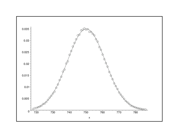
Figure 3: Comparison between Gaussian density $f(x)$ (line) and the simulation of $X^{(n)}_{3}$ (circles), with $p=1/4,n=500000$, and number of simulated words $N=200000$.

A rigorous proof of Conjecture 4.14 eludes us for now. What we have tried is the following. Define random variables $\zeta^{(n)}_{i,j}$ with the same distribution as $X^{(n)}_{i,j}$, for $n,i,j\geq 1$, but such that for fixed $n$ the random variables $(\zeta^{(n)}_{i,j})_{i,j\geq 1}$ are independent. Furthermore define $\zeta^{(n)}:=\sum_{i\neq j}\zeta^{(n)}_{i,j}$, and let $\kappa^{(n)}_{m}$, resp. $\bar{\kappa}^{(n)}_{m}$, be the $m$th cumulant of $\zeta^{(n)}$, resp. $X^{(n)}_{3}$. Then show that

1. the sequence $(\zeta^{(n)})_{n\geq 1}$ satisfies a CLT,

2. the cumulants $\kappa^{(n)}_{m}$ and $\bar{\kappa}^{(n)}_{m}$ are close enough for the CLT proof to work also for $(X^{(n)}_{3})_{n\geq 1}$.

Task i) is doable. We have $\kappa^{(n)}_{2}\sim S_{2}^{(n)}=\frac{\ln 2}{\ln^{2}q}\ln n+\mathcal{O}(1)$, by Theorem 2.1 and Lemma 4.9, and can show $\kappa^{(n)}_{m}=\mathcal{O}(\ln n)$ for $m>2$. This gives $(\kappa^{(n)}_{2})^{-\frac{m}{2}}\kappa^{(n)}_{m}\to 0$ as $n\to\infty$, for each $m>2$, therefore, by the Frechet-Shohat theorem, $(\textup{Var}\,\zeta^{(n)})^{-\frac{1}{2}}(\zeta^{(n)}-\mbox{$\mathbb{E}$}\zeta^{(n)})$ converges in distribution to a standard normal random variable. See section 4.7 in the extended preprint of Louchard et al. (2023) for first steps in the sketched direction.

For task ii), we know $|\kappa^{(n)}_{2}-\bar{\kappa}^{(n)}_{2}|\sim T^{(n)}_{2}=\mathcal{O}(1)$. Thus a bound like $|\kappa^{(n)}_{m}-\bar{\kappa}^{(n)}_{m}|=\mathcal{O}(1)$ (or even $|\kappa^{(n)}_{m}-\bar{\kappa}^{(n)}_{m}|=\mathcal{O}(\ln^{m/2-\varepsilon}n)$ with some $\varepsilon>0$) holding for $m>2$ would guarantee the above CLT argument to carry over to the sequence $(X^{(n)}_{3})_{n\geq 1}$. Now $\kappa^{(n)}_{m}-\bar{\kappa}^{(n)}_{m}$ involves infinite sums of mixed $m$th moments, and we are not quite sure, if our methods to deal with covariances would easily adapt to higher moments. Moreover the number of cases to distinguish (analogous to the 6 cases we had for $m=2$) grows rapidly with $m$. So, unfortunately, we can not report progress here.

5 Combinatorial Pattern Matching Approach

For a combinatorial approach, we utilize the methodology of Bassino et al. (2012). The full strength of Bassino et al. (2012) is not needed, because (in the present analysis) we are only studying “reduced” sets of patterns. In a reduced set of patterns, no word is a subword of another word. Here, we are always analyzing patterns of length 2, so our patterns are necessarily (already) reduced. So we only need to understand Sections 4.1 and 4.2 of Bassino et al. (2012).

Since we follow the notation and overall approach of Bassino et al. (2012), the reader might want to review the first 10 pages of Bassino et al. (2012), through Section 4.2. The basic methodology is to use an inclusion-exclusion approach to enumerating patterns. This approach allows an exact derivation of the probabilities of each set of patterns. For this approach, Section 4.1 of Bassino et al. (2012) explains how to utilize decorated texts, in which some occurrences of patterns are “distinguished” (while others might not be distinguished).

Collections of overlapping distinguished texts are gathered together into clusters. With this methodology, “the set of decorated texts $T$ decomposes as sequences of either arbitrary letters of the alphabet $\mathcal{A}$ or clusters: $T=(\mathcal{A}+C)^{*}$”. Using $\xi(z,t)=\sum_{w\in C}\pi(w)z^{|w|}t^{\tau(w)}$, where $\pi(w)$ is the probability of a text, and $\tau(w)$ is the number of distinguished occurrences of subwords in $w$, the generating function of all decorated texts is $T(z,t)=1/(1-A(z)-\xi(z,t))$.

Finally, using inclusion-exclusion, it follows that the probability generating function $F_{\mathcal{U}}(z,x)$, in which powers of $z$ mark the length of texts, and powers of $x$ mark the total number of occurrences of patterns in $\mathcal{U}$, we obtain $F_{\mathcal{U}}(z,x)=1/(1-A(z)-\xi(z,x-1))$. This is the set of core ideas from Bassino et al. (2012) that forms the foundation of the analysis in the present section.

We define $X^{(n)}$ as the total number of distinct (adjacent) pairs in a word $Z_{1},\ldots,Z_{n}$, and we have

$$X^{(n)}=\sum_{i=1}^{\infty}\sum_{j=1}^{\infty}X_{i,j}^{(n)}$$

Note 5.1

The roots of the polynomials in the denominators of the generating functions in Table 1 and in Table 2 exist and are unique (or there is a removable singularity that can be defined by using continuity).

A	gen. func.	$\frac{1}{1-z+P_{i}P_{j}z^{2}}$
	par. frac.	$\frac{1-\sqrt{1-4P_{i}P_{j}}}{2P_{i}P_{j}\sqrt{1-4P_{i}P_{j}}}\left(1-\frac{2P_{i}P_{j}}{1-\sqrt{1-4P_{i}P_{j}}}z\right)^{-1}-\frac{1+\sqrt{1-4P_{i}P_{j}}}{2P_{i}P_{j}\sqrt{1-4P_{i}P_{j}}}\left(1-\frac{2P_{i}P_{j}}{1+\sqrt{1-4P_{i}P_{j}}}z\right)^{-1}$
	coeff. of $z^{n}$	$\frac{(2P_{i}P_{j})^{n+1}}{\sqrt{1-4P_{i}P_{j}}}\bigg{(}\frac{1}{\big{(}1-\sqrt{1-4P_{i}P_{j}}\big{)}^{n+1}}-\frac{1}{\big{(}1+\sqrt{1-4P_{i}P_{j}}\big{)}^{n+1}}\bigg{)}$
B	gen. func.	$\left(1-z+\frac{P_{i}^{2}z^{2}}{1+P_{i}z}\right)^{-1}=\frac{1+P_{i}z}{1-(1-P_{i})z-P_{i}(1-P_{i})z^{2}}$
	par. frac.	$\left(\frac{1}{2}-\frac{1+P_{i}}{2\sqrt{(1-P_{i})(1+3P_{i})}}\right)\left(1-\frac{-2P_{i}(1-P_{i})}{1-P_{i}+\sqrt{(1-P_{i})(1+3P_{i})}}z\right)^{-1}$
		$\qquad\qquad{}-\left(\frac{1}{2}+\frac{1+P_{i}}{2\sqrt{(1-P_{i})(1+3P_{i})}}\right)\left(1-\frac{-2P_{i}(1-P_{i})}{1-P_{i}-\sqrt{(1-P_{i})(1+3P_{i})}}z\right)^{-1}$
	coeff. of $z^{n}$	$\left(\frac{1}{2}-\frac{1+P_{i}}{2\sqrt{(1-P_{i})(1+3P_{i})}}\right)\left(\frac{-2P_{i}(1-P_{i})}{1-P_{i}+\sqrt{(1-P_{i})(1+3P_{i})}}\right)^{n}$
		$\qquad\qquad{}-\left(\frac{1}{2}+\frac{1+P_{i}}{2\sqrt{(1-P_{i})(1+3P_{i})}}\right)\left(\frac{-2P_{i}(1-P_{i})}{1-P_{i}-\sqrt{(1-P_{i})(1+3P_{i})}}\right)^{n}$
C	gen. func.	$\frac{1}{1-z+P_{i}P_{j}z^{2}+P_{k}P_{\ell}z^{2}}$
	par. frac.	$\frac{1+\sqrt{1-4(P_{i}P_{j}\!+\!P_{k}P_{\ell})}}{2\sqrt{1-4(P_{i}P_{j}\!+\!P_{k}P_{\ell})}}\Big{(}\!1\!-\!\frac{2(P_{i}P_{j}\!+\!P_{k}P_{\ell})}{1-\sqrt{1-4(P_{i}P_{j}\!+\!P_{k}P_{\ell})}}z\!\Big{)}^{\!\!-1}\!\!\!-\!\frac{1-\sqrt{1-4(P_{i}P_{j}\!+\!P_{k}P_{\ell})}}{2\sqrt{1-4(P_{i}P_{j}\!+\!P_{k}P_{\ell})}}\Big{(}\!1\!-\!\frac{2(P_{i}P_{j}\!+\!P_{k}P_{\ell})}{1+\sqrt{1-4(P_{i}P_{j}\!+\!P_{k}P_{\ell})}}z\!\Big{)}^{\!\!-1}$
	coeff. of $z^{n}$	$\frac{(2(P_{i}P_{j}+P_{k}P_{\ell}))^{n+1}}{\sqrt{1-4(P_{i}P_{j}+P_{k}P_{\ell})}}\bigg{(}\frac{1}{\big{(}1-\sqrt{1-4(P_{i}P_{j}+P_{k}P_{\ell})}\big{)}^{n+1}}-\frac{1}{\big{(}1+\sqrt{1-4(P_{i}P_{j}+P_{k}P_{\ell})}\big{)}^{n+1}}\bigg{)}$
D	gen. func.	$\left(1-z+\frac{P_{i}z(P_{i}z+P_{\ell}z)}{1+P_{i}z}\right)^{-1}=\frac{1+P_{i}z}{1-(1-P_{i})z+(P_{i}^{2}+P_{\ell}P_{i}-P_{i})z^{2}}$
	par. frac.	$\left(\frac{1}{2}-\frac{1+P_{i}}{2\sqrt{(1-P_{i})(1+3P_{i})-4P_{i}P_{\ell}}}\right)\left(1-\frac{-2P_{i}(1-P_{i}-P_{\ell})}{1-P_{i}+\sqrt{(1-P_{i})(1+3P_{i})-4P_{i}P_{\ell}}}z\right)^{-1}$
		$\qquad\qquad{}-\left(\frac{1}{2}+\frac{1+P_{i}}{2\sqrt{(1-P_{i})(1+3P_{i})-4P_{i}P_{\ell}}}\right)\left(1-\frac{-2P_{i}(1-P_{i}-P_{\ell})}{1-P_{i}-\sqrt{(1-P_{i})(1+3P_{i})-4P_{i}P_{\ell}}}z\right)^{-1}$
	coeff. of $z^{n}$	$\left(\frac{1}{2}-\frac{1+P_{i}}{2\sqrt{(1-P_{i})(1+3P_{i})-4P_{i}P_{\ell}}}\right)\left(\frac{-2P_{i}(1-P_{i}-P_{\ell})}{1-P_{i}+\sqrt{(1-P_{i})(1+3P_{i})-4P_{i}P_{\ell}}}\right)^{n}$
		$\qquad\qquad{}-\left(\frac{1}{2}+\frac{1+P_{i}}{2\sqrt{(1-P_{i})(1+3P_{i})-4P_{i}P_{\ell}}}\right)\left(\frac{-2P_{i}(1-P_{i}-P_{\ell})}{1-P_{i}-\sqrt{(1-P_{i})(1+3P_{i})-4P_{i}P_{\ell}}}\right)^{n}$

Table 1: Table of generating functions, partial fraction decompositions, and coefficients of $z^{n}$, $n\geq 2$, in each.

E	gen. func.	$\left(1-z+\frac{P_{i}^{2}z^{2}}{1+P_{i}z}+\frac{P_{k}^{2}z^{2}}{1+P_{k}z}\right)^{-1}=\frac{(1+P_{i}z)(1+P_{k}z)}{(1-z)(1+P_{i}z)(1+P_{k}z)+P_{i}^{2}z^{2}(1+P_{k}z)+P_{k}^{2}z^{2}(1+P_{i}z)}$
	$a,b,c,d$	$a=P_{i}P_{k}(P_{i}+P_{k}-1)$, $b=P_{i}^{2}+P_{i}P_{k}+P_{k}^{2}-P_{i}-P_{k}$, $c=P_{k}+P_{i}-1$, $d=1$
	par. frac.	$\frac{(1+P_{i}z)(1+P_{k}z)}{az^{3}+bz^{2}+cz+d}$
		${}=(1+P_{i}z)(1+P_{k}z)\big{(}\frac{rs}{(r-t)(s-t)(1-z/t)}+\frac{rt}{(r-s)(t-s)(1-z/s)}+\frac{st}{(s-r)(t-r)(1-z/r)}\big{)}$
	coeff. of $z^{n}$	$\frac{(1+P_{i}t)(1+P_{k}t)rs}{(r-t)(s-t)t^{n}}+\frac{(1+P_{i}s)(1+P_{k}s)rt}{(r-s)(t-s)s^{n}}+\frac{(1+P_{i}r)(1+P_{k}r)st}{(s-r)(t-r)r^{n}}$
F	gen. func.	$\left(1-z+\frac{P_{i}^{2}z^{2}}{1+P_{i}z}+P_{k}P_{\ell}z^{2}\right)^{-1}=\frac{1+P_{i}z}{(1-z)(1+P_{i}z)+P_{i}^{2}z^{2}+P_{k}P_{\ell}z^{2}(1+P_{i}z)}$
	$a,b,c,d$	$a=P_{i}P_{k}P_{\ell}$, $b=P_{i}P_{i}+P_{k}P_{\ell}-P_{i}$, $c=P_{i}-1$, $d=1$
	par. frac.	$\frac{1+P_{i}z}{az^{3}+bz^{2}+cz+d}=(1+P_{i}z)\big{(}\frac{rs}{(r-t)(s-t)(1-z/t)}+\frac{rt}{(r-s)(t-s)(1-z/s)}+\frac{st}{(s-r)(t-r)(1-z/r)}\big{)}$
	coeff. of $z^{n}$	$\frac{(1+P_{i}t)rs}{(r-t)(s-t)t^{n}}+\frac{(1+P_{i}s)rt}{(r-s)(t-s)s^{n}}+\frac{(1+P_{i}r)st}{(s-r)(t-r)r^{n}}$
G	gen. func.	$\frac{1}{1-z+P_{i}P_{j}z^{2}+P_{j}P_{\ell}z^{2}-P_{i}P_{j}P_{\ell}z^{3}}$
	$a,b,c,d$	$a=-P_{i}P_{j}P_{\ell}$, $b=P_{i}P_{j}+P_{j}P_{\ell}$, $c=-1$, $d=1$
	par. frac.	$\frac{1}{az^{3}+bz^{2}+cz+d}=\frac{rs}{(r-t)(s-t)(1-z/t)}+\frac{rt}{(r-s)(t-s)(1-z/s)}+\frac{st}{(s-r)(t-r)(1-z/r)}$
	coeff. of $z^{n}$	$\frac{rs}{(r-t)(s-t)t^{n}}+\frac{rt}{(r-s)(t-s)s^{n}}+\frac{st}{(s-r)(t-r)r^{n}}$
H	gen. func.	$\left(1-z+\frac{2P_{i}P_{j}z^{2}}{1-P_{i}P_{j}z^{2}}-\frac{P_{i}^{2}P_{j}z^{3}}{1-P_{i}P_{j}z^{2}}-\frac{P_{i}P_{j}^{2}z^{3}}{1-P_{i}P_{j}z^{2}}\right)^{-1}=\frac{1-P_{i}P_{j}z^{2}}{(1-z)(1-P_{i}P_{j}z^{2})+2P_{i}P_{j}z^{2}-P_{i}^{2}P_{j}z^{3}-P_{i}P_{j}^{2}z^{3}}$
	$a,b,c,d$	$a=P_{i}P_{j}(1-P_{i}-P_{j})$, $b=P_{i}P_{j}$, $c=-1$, $d=1$
	par. frac.	$\frac{1-P_{i}P_{j}z^{2}}{az^{3}+bz^{2}+cz+d}=(1-P_{i}P_{j}z^{2})\big{(}\frac{rs}{(r-t)(s-t)(1-z/t)}+\frac{rt}{(r-s)(t-s)(1-z/s)}+\frac{st}{(s-r)(t-r)(1-z/r)}\big{)}$
	coeff. of $z^{n}$	$\frac{(1-P_{i}P_{j}t^{2})rs}{(r-t)(s-t)t^{n}}+\frac{(1-P_{i}P_{j}s^{2})rt}{(r-s)(t-s)s^{n}}+\frac{(1-P_{i}P_{j}r^{2})st}{(s-r)(t-r)r^{n}}$

Table 2: Table of generating functions, partial fraction decompositions, and coefficients of $z^{n}$, $n\geq 2$, in each.

Lemma 5.2

For $n\geq 2$, and for $i\neq j$, the probability that $ij$ occurs (at least once) as an adjacent pattern in $Z_{1},\ldots,Z_{n}$ is exactly

$$E[X_{i,j}^{(n)}]=1-\frac{(2P_{i}P_{j})^{n+1}}{\sqrt{1-4P_{i}P_{j}}}\Bigg{(}\frac{1}{\big{(}1-\sqrt{1-4P_{i}P_{j}}\!\ \big{)}^{n+1}}-\frac{1}{\big{(}1+\sqrt{1-4P_{i}P_{j}}\!\ \big{)}^{n+1}}\Bigg{)}.$$

Proof.   The proof of Lemma 5.2 is in subsection 5.2.1.  

Lemma 5.3

For $n\geq 2$, the probability that $ii$ occurs (at least once) as an adjacent pattern in $Z_{1},\ldots,Z_{n}$ is exactly

$$E[X_{i,i}^{(n)}] =1-\left(\frac{1}{2}-\frac{1+P_{i}}{2\sqrt{(1-P_{i})(1+3P_{i})}}\right)\left(\frac{-2P_{i}(1-P_{i})}{1-P_{i}+\sqrt{(1-P_{i})(1+3P_{i})}}\right)^{n}$$

$$\qquad\qquad{}+\left(\frac{1}{2}+\frac{1+P_{i}}{2\sqrt{(1-P_{i})(1+3P_{i})}}\right)\left(\frac{-2P_{i}(1-P_{i})}{1-P_{i}-\sqrt{(1-P_{i})(1+3P_{i})}}\right)^{n}.$$

Again, for $n<2$, we have $E[X_{i,i}^{(n)}]=0$.

Proof.   The proof of Lemma 5.3 is in subsection 5.2.2.  

5.1 Main results

By adding the results from Lemmas 5.2 and 5.3, we establish the following theorem:

Theorem 5.4

For $n\geq 2$, the mean number of distinct (adjacent) pairs in a word $Z_{1},\ldots,Z_{n}$ is exactly

$$E[X^{(n)}] =\sum_{i=1}^{\infty}\sum_{j\neq i}\Bigg{[}1-\frac{(2P_{i}P_{j})^{n+1}}{\sqrt{1-4P_{i}P_{j}}}\bigg{(}\frac{1}{\big{(}1-\sqrt{1-4P_{i}P_{j}}\!\ \big{)}^{n+1}}-\frac{1}{\big{(}1+\sqrt{1-4P_{i}P_{j}}\!\ \big{)}^{n+1}}\bigg{)}\Bigg{]}$$

$$\qquad{}+\sum_{i=1}^{\infty}\Bigg{[}1-\left(\frac{1}{2}-\frac{1+P_{i}}{2\sqrt{(1-P_{i})(1+3P_{i})}}\right)\left(\frac{-2P_{i}(1-P_{i})}{1-P_{i}+\sqrt{(1-P_{i})(1+3P_{i})}}\right)^{n}$$

$$\qquad\qquad\qquad{}+\left(\frac{1}{2}+\frac{1+P_{i}}{2\sqrt{(1-P_{i})(1+3P_{i})}}\right)\left(\frac{-2P_{i}(1-P_{i})}{1-P_{i}-\sqrt{(1-P_{i})(1+3P_{i})}}\right)^{n}\Bigg{]}$$

For $n<2$, we have $E[X^{(n)}]=0$.

In Section 5.3, we give all of the analogous parts of the analysis for $E[(X^{(n)})^{2}]$, but we do not wrap the results into a statement in a theorem, because the second moment has many parts, and the notation is cumbersome.

5.2 Analysis of the average number of distinct (adjacent) pairs

5.2.1 Analysis of distinct (adjacent) two letter patterns $ij$ with $i\neq j$

If we fix $i\neq j$ and we analyze the occurrences of the pattern $ij$, then the only “cluster” (to use Bassino et al.’s terminology) is $ij$ itself. So the generating function $\xi(z,t)$ of the set of clusters $C=\{ij\}$ becomes only (compare with (6) in Bassino et al.):

$$\xi(z,t)=P_{i}P_{j}tz^{2}.$$

The generating function of the decorated texts (with $z$ marking the length of the words, and $t$ marking the number of decorated occurrences of $ij$, and the coefficients are the associated probabilities) is

$$T(z,t)=\frac{1}{1-A(z)-\xi(z,t)}=\frac{1}{1-z-P_{i}P_{j}tz^{2}},$$

where $A(z)=z$ is the probability generating function of the alphabet $\mathcal{A}$.

Now we use $F(z,x)$ to denote the bivariate probability generating function of occurrences of $ij$ (with $z$ marking the length of the words, and $x$ marking the number of occurrences of $ij$, and the coefficients are the associated probabilities), i.e., we define

$$F(z,x):=\sum_{n=0}^{\infty}\sum_{k=0}^{\infty}P(Z_{1},\ldots,Z_{n}\textrm{ has exactly $k$ occurrences of $ij$ as a subword})x^{k}z^{n}.$$

We know from inclusion-exclusion (see (Flajolet and Sedgewick, 2009, Chapter 3) or Bassino et al. (2012)) that $F(z,x)=T(z,x-1)$, so we obtain

$$F(z,x)=T(z,x-1)=\frac{1}{1-z-P_{i}P_{j}(x-1)z^{2}}.$$

The probability generating function of words with zero occurrences of pattern $ij$ can be obtained by considering the case $k=0$, corresponding to the coefficients of $x^{0}$. To extract those coefficients, we can evaluate $F(z,x)$ at $x=0$, and we obtain

$$[x^{0}]F(z,x)=F(z,0)=\frac{1}{1-z+P_{i}P_{j}z^{2}},$$

so, finally, the probability generating function of the words with at least one occurrence of $ij$ is

$$\sum_{n=0}^{\infty}E[X_{i,j}^{(n)}]z^{n}=\frac{1}{1-z}-\frac{1}{1-z+P_{i}P_{j}z^{2}}$$

and it follows, using Table 1A, that

$$\sum_{n=0}^{\infty}E[X_{i,j}^{(n)}]z^{n} =\sum_{n=0}^{\infty}z^{n}+\frac{2P_{i}P_{j}}{(1+\sqrt{1-4P_{i}P_{j}})\sqrt{1-4P_{i}P_{j}}}\sum_{n=0}^{\infty}\bigg{(}\frac{2P_{i}P_{j}}{1+\sqrt{1-4P_{i}P_{j}}}\bigg{)}^{n}z^{n}$$

$$\qquad\qquad{}-\frac{2P_{i}P_{j}}{(1-\sqrt{1-4P_{i}P_{j}})\sqrt{1-4P_{i}P_{j}}}\sum_{n=0}^{\infty}\bigg{(}\frac{2P_{i}P_{j}}{1-\sqrt{1-4P_{i}P_{j}}}\bigg{)}^{n}z^{n}$$

and we conclude with the exact expression for $E[X_{i,j}^{(n)}]$ in Lemma 5.2.

5.2.2 Analysis of distinct (adjacent) two letter patterns $ij$ with $i=j$

Now we fix $i$ and we analyze the occurrences of the pattern $ii$. The clusters have the form $ii\cdots i$, i.e., they are all words that consist of 2 or more consecutive occurrences of $i$. So the generating function $\xi(z,t)$ of the set of clusters $C=\{ii,iii,iiii,iiiii,\ldots\}$ becomes

$$\xi(z,t)=\frac{P_{i}^{2}tz^{2}}{1-P_{i}tz}.$$

The analysis is similar to the reasoning in subsection 5.2.1, and we get

$$\sum_{n=0}^{\infty}E[X_{i,i}^{(n)}]z^{n}=\frac{1}{1-z}-\frac{1}{1-z+\frac{P_{i}^{2}z^{2}}{1+P_{i}z}}$$

and then, using Table 1B, we have

$$\sum_{n=0}^{\infty}E[X_{i,i}^{(n)}]z^{n} =\frac{1}{1-z}-\frac{(1+P_{i}z)(-1+P_{i}+\sqrt{(1-P_{i})(1+3P_{i})}\!\ )}{2\sqrt{(1-P_{i})(1+3P_{i})}\Big{(}1-\frac{-2P_{i}(1-P_{i})}{1-P_{i}+\sqrt{(1-P_{i})(1+3P_{i})}}z\Big{)}}$$

$$\qquad\qquad{}+\frac{(1+P_{i}z)(-1+P_{i}-\sqrt{(1-P_{i})(1+3P_{i})}\!\ )}{2\sqrt{(1-P_{i})(1+3P_{i})}\Big{(}1-\frac{-2P_{i}(1-P_{i})}{1-P_{i}-\sqrt{(1-P_{i})(1+3P_{i})}}z\Big{)}}$$

and we conclude with the exact expression for $E[X_{i,i}^{(n)}]$ in Lemma (5.3).

5.3 Analysis of the second moment of the number of distinct (adjacent) pairs

Now we study the second moment of $X^{(n)}$, namely, $E[(X^{(n)})^{2}]$. We have

$$(X^{(n)})^{2}=\sum_{i=1}^{\infty}\sum_{j=1}^{\infty}X_{i,j}^{(n)}\sum_{k=1}^{\infty}\sum_{\ell=1}^{\infty}X_{k,\ell}^{(n)}$$

so the second moment is, by linearity of expectation,

$$E[(X^{(n)})^{2}]=\sum_{i=1}^{\infty}\sum_{j=1}^{\infty}\sum_{k=1}^{\infty}\sum_{\ell=1}^{\infty}E[X_{i,j}^{(n)}X_{k,\ell}^{(n)}].$$

We break the analysis into 4 regimes, namely:

• $i=j$ and $k=\ell$

• $i=j$ and $k\neq\ell$

• $i\neq j$ and $k=\ell$

• $i\neq j$ and $k\neq\ell$

5.3.1 $i=j$ and $k=\ell$

In the case $i=j$ and $k=\ell$, we have two possibilities, namely, either $i=j=k=\ell$ or $i=j\neq k=\ell$.

5.3.1.1 $i=j=k=\ell$

In the case $i=j=k=\ell$, we have $X_{i,j}^{(n)}X_{k,\ell}^{(n)}=X_{i,i}^{(n)}$, so we get $E[X_{i,j}^{(n)}X_{k,\ell}^{(n)}]=E[X_{i,i}^{(n)}]$, which we already handled in Lemma 5.3.

5.3.1.2 $i=j\neq k=\ell$

In the case $i=j\neq k=\ell$, we need to analyze the occurrences of the patterns $ii$ and $kk$. The clusters each have the form $ii\cdots i$ or $kk\cdots k$, i.e., they are all words that consist of 2 or more consecutive occurrences of $i$, or consist of 2 or more consecutive occurrences of $k$. So the generating function $\xi(z,t,u)$ of the set of clusters $C=\{ii,iii,iiii,iiiii,\ldots,kk,kkk,kkkk,kkkkk,\ldots\}$ becomes

$$\xi(z,t,u)=\frac{P_{i}^{2}tz^{2}}{1-P_{i}tz}+\frac{P_{k}^{2}uz^{2}}{1-P_{k}uz}$$

(with $z$ marking the length of the words, and $t$ marking the number of decorated occurrences of $ii$, and $u$ marking the number of decorated occurrences of $kk$, and the coefficients are the associated probabilities). The methodology now proceeds in a very similar way to the method from Section 5.2.1, but $\xi$, $T$, and $F$ all have an additional variable, as compared to that earlier (more simple) analysis. We have

$$T(z,t,u)=\frac{1}{1-A(z)-\xi(z,t,u)}=\frac{1}{1-z-\frac{P_{i}^{2}tz^{2}}{1-P_{i}tz}-\frac{P_{k}^{2}uz^{2}}{1-P_{k}uz}},$$

and it follows that the probability generating function of occurrences of $ii$ and $kk$ (with $z$ marking the length of the words, and $x$ marking the number of occurrences of $ii$, and $y$ marking the number of occurrences of $kk$, and the coefficients are the associated probabilities) is

$$F(z,x,y)=T(z,x-1,y-1)=\frac{1}{1-z-\frac{P_{i}^{2}(x-1)z^{2}}{1-P_{i}(x-1)z}-\frac{P_{k}^{2}(y-1)z^{2}}{1-P_{k}(y-1)z}}.$$

It follows that the probability generating function of the words with at least one occurrence of $ii$ and at least one occurrence of $kk$ is

$$\sum_{n=0}^{\infty}E[X_{i,j}^{(n)}X_{k,\ell}^{(n)}]z^{n} =\sum_{n=0}^{\infty}E[X_{i,i}^{(n)}X_{k,k}^{(n)}]z^{n}$$

$$=\frac{1}{1-z}-F(z,0,1)-F(z,1,0)+F(z,0,0)$$

$$=\frac{1}{1-z}-\frac{1}{1-z+\frac{P_{i}^{2}z^{2}}{1+P_{i}z}}-\frac{1}{1-z+\frac{P_{k}^{2}z^{2}}{1+P_{k}z}}+\frac{1}{1-z+\frac{P_{i}^{2}z^{2}}{1+P_{i}z}+\frac{P_{k}^{2}z^{2}}{1+P_{k}z}}$$

The partial fraction decomposition for the second term is given in Table 1B.

The third term is the same as the second term, using $k$ instead of $i$.

The partial fraction decomposition for the fourth term is given in Table 2E.

5.3.2 $i=j$ and $k\neq\ell$

5.3.2.1 $i=j$ and $k$ and $\ell$ are distinct

The clusters each have the form $ii\cdots i$ or $k\ell$, i.e., they are all words that consist of either 2 or more consecutive occurrences of $i$, or simply the word $k\ell$. So $\xi(z,t,u)$ of the set of clusters $C=\{ii,iii,iiii,iiiii,\ldots,k\ell\}$ becomes

$$\xi(z,t,u)=\frac{P_{i}^{2}tz^{2}}{1-P_{i}tz}+P_{k}P_{\ell}uz^{2}$$

(with $z$ marking the length of the words, and $t$ marking the number of decorated occurrences of $ij$, and $u$ marking the number of decorated occurrences of $k\ell$, and the coefficients are the associated probabilities). It follows that

$$T(z,t,u) =\frac{1}{1-z-\frac{P_{i}^{2}tz^{2}}{1-P_{i}tz}-P_{k}P_{\ell}uz^{2}},$$

and

$$F(z,x,y)=T(z,x-1,y-1)=\frac{1}{1-z-\frac{P_{i}^{2}(x-1)z^{2}}{1-P_{i}(x-1)z}-P_{k}P_{\ell}(y-1)z^{2}}.$$

It follows that the probability generating function of the words with at least one occurrence of $ij$ and at least one occurrence of $k\ell$ is

$$\sum_{n=0}^{\infty}E[X_{i,j}^{(n)}X_{k,\ell}^{(n)}]z^{n} =\frac{1}{1-z}-F(z,0,1)-F(z,1,0)+F(z,0,0)$$

$$=\frac{1}{1-z}-\frac{1}{1-z+\frac{P_{i}^{2}z^{2}}{1+P_{i}z}}-\frac{1}{1-z+P_{k}P_{\ell}z^{2}}+\frac{1}{1-z+\frac{P_{i}^{2}z^{2}}{1+P_{i}z}+P_{k}P_{\ell}z^{2}}$$

The partial fraction decomposition for the second term is given in Table 1B.

The partial fraction decomposition for the third term is given in Table 1A, using $k$ and $\ell$ instead of $i$ and $j$.

The partial fraction decomposition for the fourth term is given in Table 2F.

5.3.2.2 $i=j=k\neq\ell$

The clusters each have the form $ii\cdots i$ or $ii\cdots i\ell$, i.e., they are all words that consist of 2 or more consecutive occurrences of $i$, or of 1 or more consecutive occurrences of $i$ followed by $\ell$. So $\xi(z,t,u)$ of the set of clusters $C=\{ii,iii,iiii,iiiii,\ldots,i\ell,ii\ell,iii\ell,iiii\ell,\ldots\}$ becomes

$$\xi(z,t,u)=\frac{P_{i}^{2}tz^{2}}{1-P_{i}tz}+\frac{P_{i}P_{\ell}uz^{2}}{1-P_{i}tz}=\frac{P_{i}z(P_{i}tz+P_{\ell}uz)}{1-P_{i}tz},$$

and

$$F(z,x,y)=\frac{1}{1-z-\frac{P_{i}z(P_{i}(x-1)z+P_{\ell}(y-1)z)}{1-P_{i}(x-1)z}}.$$

It follows that the probability generating function of the words with at least one occurrence of $ij$ and at least one occurrence of $k\ell$ is

$$\sum_{n=0}^{\infty}E[X_{i,j}^{(n)}X_{k,\ell}^{(n)}]z^{n} =\frac{1}{1-z}-F(z,0,1)-F(z,1,0)+F(z,0,0)$$

$$=\frac{1}{1-z}-\frac{1}{1-z+\frac{P_{i}^{2}z^{2}}{1+P_{i}z}}-\frac{1}{1-z+P_{i}P_{\ell}z^{2}}+\frac{1}{1-z+\frac{P_{i}z(P_{i}z+P_{\ell}z)}{1+P_{i}z}}$$

The partial fraction decomposition for the second term is given in Table 1B.

The partial fraction decomposition for the third term is given in Table 1A, using $\ell$ instead of $j$.

The partial fraction decomposition for the fourth term is given in Table 1D.

5.3.2.3 $i=j=\ell\neq k$

The cluster have the form $ki\cdots i$ or $ii\cdots i$, i.e., they are all words that consist of $k$ followed by 1 or more consecutive occurrences of $i$, or of 2 or more consecutive occurrences of $i$. So $\xi(z,t,u)$ of the set of clusters $C=\{ki,kii,kiii,kiiii,\ldots,ii,iii,iiii,iiiii,\ldots\}$ becomes

$$\xi(z,t,u)=\frac{P_{i}P_{k}uz^{2}}{1-P_{i}tz}+\frac{P_{i}^{2}tz^{2}}{1-P_{i}tz}=\frac{P_{i}z(P_{k}uz+P_{i}tz)}{1-P_{i}tz},$$

and

$$F(z,x,y)=\frac{1}{1-z-\frac{P_{i}z(P_{k}(y-1)z+P_{i}(x-1)z)}{1-P_{i}(x-1)z}}.$$

It follows that the probability generating function of the words with at least one occurrence of $ij$ and at least one occurrence of $k\ell$ is

$$\sum_{n=0}^{\infty}E[X_{i,j}^{(n)}X_{k,\ell}^{(n)}]z^{n} =\frac{1}{1-z}-F(z,0,1)-F(z,1,0)+F(z,0,0)$$

$$=\frac{1}{1-z}-\frac{1}{1-z+\frac{P_{i}^{2}z^{2}}{1+P_{i}z}}-\frac{1}{1-z+P_{i}P_{k}z^{2}}+\frac{1}{1-z+\frac{P_{i}z(P_{k}z+P_{i}z)}{1+P_{i}z}}$$

The partial fraction decomposition for the second term is given in Table 1B.

The partial fraction decomposition for the third term is given in Table 1A, using $k$ instead of $j$.

The partial fraction decomposition for the fourth term is given in Table 1D, using $k$ instead of $\ell$.

5.3.3 $i\neq j$ and $k=\ell$

5.3.3.1 $k=\ell$ and $i$ and $j$ are distinct

Same as section 5.3.2.1 but with $i$ and $k$ exchanged, and with $j$ and $\ell$ exchanged.

5.3.3.2 $k=\ell=i\neq j$

Same as section 5.3.2.2 but with $i$ and $k$ exchanged, and with $j$ and $\ell$ exchanged.

5.3.3.3 $k=\ell=j\neq i$

Same as section 5.3.2.3 but with $i$ and $k$ exchanged, and with $j$ and $\ell$ exchanged.

5.3.4 $i\neq j$ and $k\neq\ell$

5.3.4.1 $i$ and $j$ and $k$ and $\ell$ are distinct

The clusters are $ij$ and $k\ell$. So $\xi(z,t,u)$ of the set of clusters $C=\{ij,k\ell\}$ becomes

$$\xi(z,t,u)=P_{i}P_{j}tz^{2}+P_{k}P_{\ell}uz^{2},$$

and

$$F(z,x,y)=\frac{1}{1-z-P_{i}P_{j}(x-1)z^{2}-P_{k}P_{\ell}(y-1)z^{2}}.$$

It follows that the probability generating function of the words with at least one occurrence of $ij$ and at least one occurrence of $k\ell$ is

$$\sum_{n=0}^{\infty}E[X_{i,j}^{(n)}X_{k,\ell}^{(n)}]z^{n} =\frac{1}{1-z}-F(z,0,1)-F(z,1,0)+F(z,0,0)$$

$$=\frac{1}{1-z}-\frac{1}{1-z+P_{i}P_{j}z^{2}}-\frac{1}{1-z+P_{k}P_{\ell}z^{2}}$$

$$\qquad{}+\frac{1}{1-z+P_{i}P_{j}z^{2}+P_{k}P_{\ell}z^{2}}$$

The partial fraction decomposition for the second term is given in Table 1A.

The partial fraction decomposition for the third term is given in Table 1A, using $k$ and $\ell$ instead of $i$ and $j$.

The partial fraction decomposition for the fourth term is given in Table 1C.

5.3.4.2 $k=i$ and $j$ and $\ell$ are distinct

The clusters are $ij$ and $i\ell$. So, by the same analysis from section 5.3.4.1, we get

$$\sum_{n=0}^{\infty}E[X_{i,j}^{(n)}X_{i,\ell}^{(n)}]z^{n} =\frac{1}{1-z}-F(z,0,1)-F(z,1,0)+F(z,0,0)$$

$$=\frac{1}{1-z}-\frac{1}{1-z+P_{i}P_{j}z^{2}}-\frac{1}{1-z+P_{i}P_{\ell}z^{2}}$$

$$\qquad{}+\frac{1}{1-z+P_{i}P_{j}z^{2}+P_{i}P_{\ell}z^{2}}$$

Exactly as in section 5.3.4.1 above:

The partial fraction decomposition for the second term is given in Table 1A.

The partial fraction decomposition for the third term is given in Table 1A, using $\ell$ instead of $j$.

The partial fraction decomposition for the fourth term is given in Table 1C, using $i$ instead of $k$.

5.3.4.3 $k=j$ and $i$ and $\ell$ are distinct

The clusters are $ij$, $ij\ell$ and $j\ell$. So $\xi(z,t,u)$ of the set of clusters $C=\{ij,ij\ell,j\ell\}$ becomes

$$\xi(z,t,u)=P_{i}P_{j}tz^{2}+P_{j}P_{\ell}uz^{2}+P_{i}P_{j}P_{\ell}tuz^{3},$$

and

$$F(z,x,y)=\frac{1}{1-z-P_{i}P_{j}(x-1)z^{2}-P_{j}P_{\ell}(y-1)z^{2}-P_{i}P_{j}P_{\ell}(x-1)(y-1)z^{3}}.$$

It follows that the probability generating function of the words with at least one occurrence of $ij$ and at least one occurrence of $j\ell$ is

$$\sum_{n=0}^{\infty}E[X_{i,j}^{(n)}X_{j,\ell}^{(n)}]z^{n} =\frac{1}{1-z}-F(z,0,1)-F(z,1,0)+F(z,0,0)$$

$$=\frac{1}{1-z}-\frac{1}{1\!-\!z\!+\!P_{i}P_{j}z^{2}}-\frac{1}{1\!-\!z\!+\!P_{j}P_{\ell}z^{2}}+\frac{1}{1-z+P_{i}P_{j}z^{2}+P_{j}P_{\ell}z^{2}-P_{i}P_{j}P_{\ell}z^{3}}$$

The partial fraction decompositions for the second and third terms are given in Table 1A, once using $j$ and $\ell$ instead of $i$ and $j$.

The partial fraction decomposition for the fourth term is given in Table 2G.

5.3.4.4 $i=\ell$ and $k$ and $j$ are distinct

Same as section 5.3.4.3 but with $i$ and $k$ exchanged, and with $j$ and $\ell$ exchanged.

5.3.4.5 $\ell=j$ and $i$ and $k$ are distinct

The clusters are $ij$ and $kj$. So, by the same analysis from section 5.3.4.1, we get

$$\sum_{n=0}^{\infty}E[X_{i,j}^{(n)}X_{k,j}^{(n)}]z^{n} =\frac{1}{1-z}-F(z,0,1)-F(z,1,0)+F(z,0,0)$$

$$=\frac{1}{1-z}-\frac{1}{1-z+P_{i}P_{j}z^{2}}-\frac{1}{1-z+P_{k}P_{j}z^{2}}$$

$$\qquad{}+\frac{1}{1-z+P_{i}P_{j}z^{2}+P_{k}P_{j}z^{2}}$$

Exactly as in section 5.3.4.1 above:

The partial fraction decomposition for the second term is given in Table 1A.

The partial fraction decomposition for the third term is given in Table 1A, using $k$ instead of $i$.

The partial fraction decomposition for the fourth term is given in Table 1C, using $j$ instead of $\ell$.

5.3.4.6 $i=k$ and $j=\ell$ are distinct

In this case we have $X_{i,j}^{(n)}X_{k,\ell}^{(n)}=X_{i,j}^{(n)}$, so we get $E[X_{i,j}^{(n)}X_{k,\ell}^{(n)}]=E[X_{i,j}^{(n)}]$, which we already handled in Lemma 5.2.

5.3.4.7 $i=\ell$ and $j=k$ are distinct

The clusters each have the form $ijiji\ldots$ or $jijij\ldots$. So $\xi(z,t,u)$ of the set of clusters $C=\{ij,iji,ijij,ijiji\ldots,ji,jij,jiji,jijij\ldots\}$ becomes

$$\xi(z,t,u)=\frac{P_{i}P_{j}tz^{2}}{1-P_{i}P_{j}tuz^{2}}+\frac{P_{i}^{2}P_{j}tuz^{3}}{1-P_{i}P_{j}tuz^{2}}+\frac{P_{j}P_{i}uz^{2}}{1-P_{i}P_{j}tuz^{2}}+\frac{P_{i}P_{j}^{2}tuz^{3}}{1-P_{i}P_{j}tuz^{2}},$$

and $F(z,x,y)=1/(1-z-\xi(z,x-1,y-1))$. It follows that the probability generating function of the words with at least one occurrence of $ij$ and at least one occurrence of $k\ell$ is

$$\sum_{n=0}^{\infty}E[X_{i,j}^{(n)}X_{k,\ell}^{(n)}]z^{n} =\frac{1}{1-z}-F(z,0,1)-F(z,1,0)+F(z,0,0)$$

$$=\frac{1}{1-z}-\frac{1}{1-z+P_{i}P_{j}z^{2}}-\frac{1}{1-z+P_{j}P_{i}z^{2}}$$

$$\qquad{}+\frac{1}{1-z+\frac{P_{i}P_{j}z^{2}}{1-P_{i}P_{j}z^{2}}-\frac{P_{i}^{2}P_{j}z^{3}}{1-P_{i}P_{j}z^{2}}+\frac{P_{j}P_{i}z^{2}}{1-P_{i}P_{j}z^{2}}-\frac{P_{i}P_{j}^{2}z^{3}}{1-P_{i}P_{j}z^{2}}}$$

The partial fraction decomposition for the second and for the third term is given in Table 1A.

The partial fraction decomposition for the fourth term is given in Table 2H.

As mentioned immediately after Theorem 5.4, we do not wrap all of the analysis from Section 5.3 into a theorem (because it would be very lengthy), but we have precisely analyzed every aspect that is needed for exactly characterizing the second moment $E[(X^{(n)})^{2}]$.

Appendix A Some Mellin transforms

To keep the paper self contained we give here a short outline on how to use Mellin transforms to obtain asymptotic expansions. The reader seeking more detail is referred to Flajolet et al. (1995) for a nice exposition. Subsections A.1, A.2, and A.3 are devoted to asymptotic equivalents of three sums that play a crucial role in our paper.

The Mellin transform $f^{*}(s)$ of $f(x)$, also denoted $\mathcal{M}\left[f(x);s\right]$, is given by

$$f^{*}(s)=\int_{0}^{\infty}f(x)x^{s-1}dx.$$

The interior of the set of $s$ for which the integral converges is an open strip $\langle a,b\rangle:=\{s\in\mathbb{C}:a<\Re s<b\}$, called the fundamental strip, with $a,b$ depending on how $f$ behaves at $0$ and $\infty$. For example, we have $\mathcal{M}\left[e^{-x};s\right]=\Gamma(s)$, with fundamental strip $\langle 0,\infty\rangle$, and $\mathcal{M}\left[1-e^{-x};s\right]=-\Gamma(s)$, with fundamental strip $\langle-1,0\rangle$. When computing the Mellin transform of so called harmonic sums, the rescaling rule turns out to be very useful:

$$\mathcal{M}\left[\sum_{k}\lambda_{k}f(\mu_{k}x);s\right]=\sum_{k}\frac{\lambda_{k}}{\mu_{k}^{s}}\cdot f^{*}(s).$$

In the case that $f^{*}(s)$ can be meromorphically continued to a strip $\langle a,\bar{b}\rangle$ with $\bar{b}>b$, information on the poles of $f^{*}(s)$ leads to asymptotic properties of $f(n),n\rightarrow\infty$. This is called the fundamental correspondence. In particular, if there is a pole

$$\frac{1}{(s-\xi)^{k+1}}$$

of $f^{*}(s)$ at $\xi=\sigma+\mathbf{i}t$ to the right of the fundamental strip, then this pole will contribute the term

$$-\frac{(-1)^{k}}{k!}\ln(n)^{k}n^{-\sigma}e^{-\mathbf{i}t\ln(n)},$$

which is precisely the residue of $\frac{-n^{-s}}{(s-\xi)^{k+1}}$ at $s=\xi$, to an asymptotic expansion of $f(n)$ at $\infty$. Justification comes from residue calculus: If $f$ is smooth enough, the inverse transform applies to yield $f(n)=\frac{1}{2\pi\mathbf{i}}\int_{c-\mathbf{i}\infty}^{c+\mathbf{i}\infty}n^{-s}f^{*}(s)ds$ with $a<c<b$. If for $\beta<\bar{b}$ the set of poles $z$ in $\langle a,\bar{b}\rangle$ satisfying $\Re z<\beta$ is denoted $\mathcal{S}_{\beta}$, and there is no pole with real part $\beta$, we have

$$f(n)=\frac{1}{2\pi\mathbf{i}}\int_{\beta-\mathbf{i}\infty}^{\beta+\mathbf{i}\infty}n^{-s}f^{*}(s)ds-\sum_{z\in\mathcal{S}_{\beta}}\textup{Res}(f^{*}(s)n^{-s})_{s=z}=-\sum_{z\in\mathcal{S}_{\beta}}\textup{Res}(f^{*}(s)n^{-s})_{s=z}+\mathcal{O}(n^{-\beta}),$$

with the integral being $\mathcal{O}(n^{-\beta})$, provided that $f^{*}(s)$ decreases fast enough for $s=\beta+\mathbf{i}t$ and $|t|\to\infty$. Equality of left and right hand side is established by using a sequence of contours $\rho_{k}$ being the boundaries of rectangles $\{z\in\mathbb{C}:c\leq\Re z\leq\beta,-h_{k}\leq\Im z\leq h_{k}\}$ with $h_{k}\to\infty$, verifying that $f^{*}(s)$ decreases fast enough on the horizontal segments of $\rho_{k}$, as $k\to\infty$, and applying residue calculus.

Here is an illustration of fast enough decrease. $\Gamma(s)$ decreases exponentially in the direction $\mathbf{i}\infty$:

$$|\Gamma(\sigma+\mathbf{i}t)|\sim\sqrt{2\pi}|t|^{\sigma-1/2}e^{-\pi|t|/2}.$$

Also, similarly fast decrease can be observed for all other transforms we encounter.

In the following, recall the notations

$$L:=\ln\tfrac{1}{q}\mbox{ and }\chi:=\tfrac{2\mathbf{i}\pi}{L}.$$

A.1

Let

$$G(n):=\sum_{i\geq 0}\left(1-e^{-nq^{2i}}\right).$$

The Mellin transform of this sum is $G^{*}(s)=-\dfrac{1}{1-q^{-2s}}\Gamma(s)$, with fundamental strip $\langle-1,0\rangle$, to the right of which the meromorphic extension of $G^{*}(s)$ has poles at $s=0$ and $s=\frac{\ell\chi}{2}$ for $\ell\in\mbox{$\mathbb{Z}$}\setminus\{0\}$, with singular expansions

$$G^{*}(s)\asymp\frac{1}{2Ls^{2}}-\left[\frac{\gamma}{2L}+\frac{1}{2}\right]\frac{1}{s},\quad\mbox{ and }G^{*}(s)\asymp\frac{1}{2L}\frac{\Gamma\big{(}\frac{\ell\chi}{2}\big{)}}{\big{(}s-\frac{\ell\chi}{2}\big{)}},\mbox{ for }\ell\in\mbox{$\mathbb{Z}$}\setminus\{0\}.$$

Noting that there are no other singularities to the right of $\langle-1,0\rangle$, the error term in the following expansion can be chosen $\mathcal{O}(n^{-\beta})$ with any fixed $\beta>0$.

$$G(n)\sim\frac{1}{2L}\ln(n)+\left[\frac{\gamma}{2L}+\frac{1}{2}\right]-\frac{1}{2L}\sum_{\ell\in\mbox{$\mathbb{Z}$}\setminus\{0\}}\Gamma\Big{(}\frac{\ell\chi}{2}\Big{)}n^{-\ell\chi/2}.$$

A.2

Let

$$\tilde{G}(n):=\sum_{i,j\geq 0}\left(1-e^{-nq^{i+j}}\right)=\sum_{k\geq 0}(k+1)\left(1-e^{-nq^{k}}\right).$$

Here we have $\tilde{G}^{*}(s)=-\dfrac{1}{(1-q^{-s})^{2}}\Gamma(s)$, with fundamental strip $\langle-1,0\rangle$, and poles at $s=0$ and $s=\ell\chi$ for $\ell\in\mbox{$\mathbb{Z}$}\setminus\{0\}$, with singular expansions

$$\tilde{G}^{*}(s)\asymp-\frac{1}{L^{2}s^{3}}+\left[\frac{\gamma}{L^{2}}+\frac{1}{L}\right]\frac{1}{s^{2}}-\left[\frac{\pi^{2}+6\gamma^{2}}{12L^{2}}+\frac{5}{12}+\frac{\gamma}{L}\right]\frac{1}{s},$$

and

$$\tilde{G}^{*}(s)\asymp-\frac{\Gamma(\ell\chi)}{L^{2}(s-\ell\chi)^{2}}-\frac{\Gamma^{\prime}(\ell\chi)-L\Gamma(\ell\chi)}{L^{2}(s-\ell\chi)},\mbox{ for }\ell\in\mbox{$\mathbb{Z}$}\setminus\{0\},$$

leading to

$$\tilde{G}(n)\sim\frac{\ln(n)^{2}}{2L^{2}}+\left[\frac{\gamma}{L^{2}}+\frac{1}{L}\right]\ln(n)+\left[\frac{\pi^{2}+6\gamma^{2}}{12L^{2}}+\frac{5}{12}+\frac{\gamma}{L}\right]+\frac{1}{L^{2}}\!\!\!\sum_{\ell\in\mbox{$\mathbb{Z}$}\setminus\{0\}}\!\!\!\!\!\!\left[\Gamma^{\prime}\left(\ell\chi\right)-(\ln(n)+L)\Gamma\left(\ell\chi\right)\right]n^{-\ell\chi},$$

again with error term $\mathcal{O}(n^{-\beta})$ with any fixed $\beta>0$.

A.3

Set

$$\hat{G}(n):=\sum_{i,j,k}(e^{nP_{i}P_{j}P_{k}}-1)e^{-nP_{i}P_{j}-nP_{j}P_{k}}.$$

This leads to the Mellin transform, with fundamental strip $\langle-1,0\rangle$,

$$\hat{G}^{*}(s)= \sum_{i,j,k}\int_{0}^{\infty}(e^{xP_{i}P_{j}P_{k}}-1)e^{-xP_{i}P_{j}-xP_{j}P_{k}}x^{s-1}dx$$

$$= \sum_{j}P_{j}^{-s}\sum_{i,k}\int_{0}^{\infty}\left[e^{-y(P_{i}+P_{k}-P_{i}P_{k})}-e^{-y(P_{i}+P_{k})}\right]y^{s-1}dy$$

$$= \frac{q^{s}}{p^{s}(q^{s}-1)}\Gamma(s)\sum_{i,k}\left[(P_{i}+P_{k}-P_{i}P_{k})^{-s}-(P_{i}+P_{k})^{-s}\right]$$

$$= \left(\frac{q}{p}\right)^{2s}\frac{\Gamma(s)}{q^{s}-1}F_{1}(s),$$

where

$$F_{1}(s) =\sum_{i,k}\left[(q^{i}+q^{k}-pq^{i+k-1})^{-s}-(q^{i}+q^{k})^{-s}\right]$$

$$=\sum_{i\geq 1}q^{-is}\left[(2-P_{i})^{-s}-2^{-s}+2\sum_{j\geq 1}\left[(1+q^{j}-pq^{i+j-1})^{-s}-(1+q^{j})^{-s}\right]\right].$$

Note that $F_{1}(s)$, being a general Dirichlet series in the variable $-s$, is analytic at least for $\sigma=\Re s<1$, since, using the Mean Value Theorem, we have

$$\left|(1+q^{j}-pq^{i+j-1})^{-\sigma}-(1+q^{j})^{-\sigma}\right|\leq|\sigma|\frac{pq^{i+j-1}}{(1+q^{j})^{1+\sigma}},$$

and therefore

$$|F_{1}(s)|\leq 2|\sigma|\sum_{i\geq 1}q^{i(1-\sigma)}\sum_{j\geq 0}\frac{P_{j}}{(1+q^{j})^{1+\sigma}}<\infty.$$

Moreover, $F_{1}(0)=0$, so to the right of the fundamental strip we have the singular expansions

$$\hat{G}^{*}(s)\asymp-\frac{F^{\prime}_{1}(0)}{Ls},\quad\textup{and}\ \hat{G}^{*}(s)\asymp-p^{-2\ell\chi}\frac{\Gamma(\ell\chi)}{L}\frac{F_{1}(\ell\chi)}{s-\ell\chi},\ \textup{for}\ \ell\in\mathbb{Z}\setminus\{0\}.$$

This leads to

$$\hat{G}(n)=\frac{F^{\prime}_{1}(0)}{L}+\frac{1}{L}\sum_{\ell\in\mbox{$\mathbb{Z}$}\setminus\{0\}}\Gamma(\ell\chi)F_{1}(\ell\chi)(np^{2})^{-\ell\chi}+\mathcal{O}(n^{-\beta}),$$

with any fixed $\beta<1$, where the constant term simplifies to

$$\frac{F^{\prime}_{1}(0)}{L}=\frac{1}{L}\ln\Bigg{(}\prod_{i,k\geq 1}\frac{q^{i}+q^{k}}{q^{i}+q^{k}-pq^{i+k-1}}\Bigg{)}.$$