Non-perturbative renormalization of the QCD flavour-singlet local vector current
Abstract
We compute non-perturbatively the renormalization constant of the flavour-singlet local vector current in lattice QCD with 3 massless flavours. Gluons are discretized by the Wilson plaquette action while quarks by the O()-improved Wilson–Dirac operator. The constant is fixed by comparing the expectation values (1-point functions) of the conserved and local vector currents at finite temperature in the presence of shifted boundary conditions and at non-zero imaginary chemical potential. Monte Carlo simulations with a moderate computational cost allow us to obtain with an accuracy of about 8‰ for values of the inverse bare coupling constant in the range .
1 Introduction
Lattice Quantum Chromodynamics (QCD) allows us to compute non-perturbatively physically relevant matrix elements of composite operators from first principles. If not related to a conserved lattice symmetry, composite fields need to be renormalized non-perturbatively before taking the continuum limit of lattice results. The Schrödinger Functional [1], the RI-MOM [2], and the Wilson flow [3] schemes and their variants have been proposed in the past to accomplish that task.
Computing renormalization constants can be a numerically demanding problem since one often has to measure correlation functions of two or more operators at a physical distance. The calculation becomes even more challenging when there are contributions from disconnected Wick contractions of fermion propagators: in fact, in these cases, the signal decreases with the distance between the fields while the statistical fluctuations stay constant. This is the main reason for which there is a paucity of results in the literature on the renormalization constants of flavour-singlet operators.
Recently a non-perturbative renormalization framework has been proposed based on considering the field theory at finite temperature in the presence of non-trivial boundary conditions in the compact direction [4, 5, 6]. In this scheme the renormalization constants of what becomes a conserved charge111Extensions to other operators deserve dedicated investigations which go beyond the scope of this letter. in the continuum limit can be computed by considering 1-point functions in the presence of non-trivial boundary conditions allowed by the residual lattice symmetry associated to that charge, a fact that reduces very significantly the numerical effort to attain a given accuracy on the renormalization constants. For flavour-singlet operators this is even more so because the 1-point functions do not suffer from the degradation of the signal to noise ratio with the distance of the inserted fields.
The use of thermal QCD in the presence of shifted boundary conditions [7, 8, 4] solved the problem of renormalizing non-perturbatively the energy-momentum tensor in the SU() Yang-Mills theory by leading to a determination of its renormalization constants with a sub-percent precision [5]. Our long-term goal is to generalize these findings to QCD. In this case the renormalization of the energy-momentum tensor is complicated by the mixing between two operators, the gluonic and the fermion components, a problem which can be solved by introducing a twist phase for fermions at the boundaries (or equivalently an imaginary chemical potential) in addition to the shift [6].
Before addressing our main task, maybe the simplest application to explore the effectiveness of using an imaginary chemical potential for renormalizing composite operators is the computation of the renormalization constant of the flavour-singlet local vector current. This problem on the one hand is simpler because the operator is multiplicatively renormalizable and it can be matched to the corresponding non-local conserved current, but on the other hand the difficulty of computing the disconnected Wick contractions remains intact. Some results have been obtained with staggered fermions [9] and with Wilson fermions for one lattice ensemble [10] using the approach proposed in [2].
The aim of this letter is to compute non-perturbatively the renormalization constant of the flavour-singlet local vector current in lattice QCD with 3 massless flavours in a wide range of values of the gauge coupling. Apart for its intrinsic theoretical interest, this allows us to test several main ingredients of the renormalization strategy based on shifted and twisted boundary conditions for fermions [6]. It must be said that the non-perturbative renormalization of local vector currents on the lattice has been a topic of interest for quite some time [11, 12] until recent investigations [13, 14, 15]. Indeed, the vector currents are crucial operators in many open physics problems, e.g. the calculation of the Hadronic Vacuum Polarization contribution to the anomalous magnetic moment of the muon [16].
This letter is organized as follows. In Section 2 we introduce the renormalization scheme we are interested in, the notation, and the definition of the renormalization constant of the flavour-singlet local vector current. In Section 3 we present the results of our numerical study, and in particular our best parameterization for . Finally, in the last Section, we conclude the paper with our view on possible future applications of this renormalization scheme. In a couple of appendices we collect the details of the lattice action that we have used in the Monte Carlo simulations, and the 1-loop perturbative results that we have derived in order to improve the definition of and consequently our numerical results.
2 Thermal Lattice QCD and renormalization
Lattice QCD at finite temperature is usually studied with the purpose of computing thermodynamical quantities like, for instance, the pressure, the entropy density, the energy density as well as screening masses, transport coefficients or other physically interesting observables. In this letter, instead, we consider thermal QCD for defining and computing the renormalization constant of the flavour-singlet local vector current on the lattice. Being conserved in the continuum, its renormalization constant depends on the specific definitions of the operator and of the action on the lattice while, up to discretization effects, is independent on the particular renormalization condition adopted.
We focus on lattice QCD with flavours of O()-improved clover massless quarks [17], and we consider the Wilson plaquette action for the gauge sector. We refer readers to A for the conventions adopted, for a detailed definition of the action, and for the tuning of the improvement coefficient of the Dirac operator and of the quark mass to its critical value. The theory is formulated in a moving reference frame [7, 8, 4], which corresponds to impose on the fields periodic boundary conditions in the compact direction up to a spatial shift . Hence, the gauge field and the quark and the anti-quark triplets and satisfy the following boundary conditions
| (1) | ||||
respectively, where , and is the lattice size in the temporal direction. In the spatial directions all fields are periodic. In Eq. (1) we have considered for the fermion fields also a non trivial twist phase in addition to the usual antiperiodicity [6]. It can be shown that, by a change of variables, the twist phase can be rewritten as an imaginary chemical potential [18], in the presence of which it is known that there is an effective periodicity of the free energy due to the interplay of with the centre symmetry of the SU() pure gauge sector [19].
The vector subgroup of the chiral symmetry of QCD is not broken by the Wilson discretization of fermions, and therefore it holds also at finite lattice spacing with degenerate quarks. As a consequence, there is a conserved flavour-singlet vector current which is defined as
| (2) |
where are the Dirac matrices and indicates the unit vector oriented along the direction . The current has a unit renormalization constant, and it approaches the continuum one in the limit of vanishing lattice spacing . However, other discretizations of the flavour-singlet vector current on the lattice can also be studied like, for instance, the one that more closely resembles the continuum definition
| (3) |
Although the use of requires the computation of its renormalization constant , it has the appealing numerical feature of involving fields on a single lattice point which often implies smaller statistical fluctuations of correlators and smaller lattice artifacts. Moreover, having two definitions of the current turns out to be useful in many cases, e.g. for constraining the extrapolation of lattice results with different discretization effects to the same continuum limit [20].
Using the change of variables that we mentioned above to trade off the twist phase at the boundary of the compact direction for an imaginary chemical potential in the bulk, in [6] we show that the expectation value of the temporal component of the conserved current is related to the derivative with respect to of the free-energy density of a system at temperature with
| (4) |
There is no dependence on the position of the current thanks to the translational invariance of the theory. For Eq. (4) not to be trivial, i.e. for having a non vanishing expectation value of the temporal component of the current, the twist phase has to be different from zero. This is the reason for considering a non null twist phase in Eq. (1).
Since the lattice action is O()-improved, discretization effects in the free-energy start at O(). Eq. (4) then implies that the expectation value of the conserved current on the l.h.s. is O()-improved. This is consistent with the Symanzik effective field theory analysis. Indeed in the chiral limit and when inserted in correlators at a physical distance from other fields, either the conserved or the local vector currents in Eqs. (2) and (3) can be improved by adding a single dimension- operator related to the tensor current [21]. The resulting O()-improved operators read
| (5) |
where and are the forward and the backward lattice derivatives. The numerical coefficients need to be properly tuned in order to accomplish the non-perturbative improvement. However, since we are interested in their 1-point functions only, the contribution coming from the improvement terms vanish due to the translation invariance, and the expectation values of both the local (once properly renormalized) and the conserved vector currents are O()-improved as they stand.
The above analysis suggests to define the renormalization constant of the flavour-singlet local vector current as
| (6) |
where the limit is taken at fixed spacing (i.e. fixed bare coupling ) and the expectation values are computed in the thermodynamic limit. Since the vector current does not need renormalization in the continuum, the ratio on the r.h.s. in Eq. (6) depends on the twist phase and on the shift only because of discretization effects, a dependence which goes away when the limit is taken. The residual (small) O() discretization effects are part of the definition of the renormalization constant, and we omit to indicate them explicitly throughout the letter. As usual, they will be removed when taking the continuum limit of correlators with the renormalized flavour-singlet local vector current inserted.
We indicate the ratio at fixed by . Its value at tree-level in perturbation theory, , is shown in Figure 1 as a function of , for several values of and for the two shifts (top panel) and (bottom panel). When becomes smaller and smaller, approaches the asymptotic value of quadratically in . Discretization effects turn out to be one order of magnitude smaller for the shift with respect to the case of periodic boundary conditions, a fact which is confirmed also at the next order in the perturbative expansion. This is the reason why we have selected the shift for carrying out the non-perturbative calculation. A similar reduction of lattice artifacts for was observed in the computation of the entropy density in the SU() Yang-Mills theory [22, 23] and of the QCD mesonic screening masses [24].
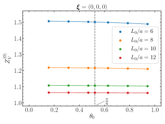
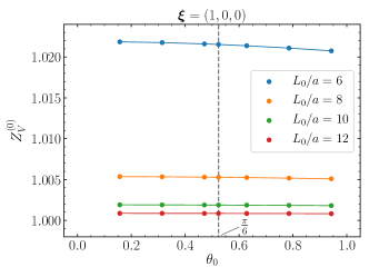
The dependence of discretization effects on , instead, is very mild and we have chosen to perform the numerical simulations at : this is the middle of the range of non trivial values since the partition function is even in .
Before carrying out the non-perturbative computation, we have computed in lattice perturbation theory up to O() in the thermodynamic limit. This serves to confirm our choices for the values of the shift and of the twist phase, and it allows us to introduce a perturbatively improved definition of the renormalization constant which reads
| (7) |
The 1-loop coefficient is [25, 26]
| (8) |
where the Sheikholeslami-Wohlert term [17] has been also taken into account and whose coefficient at O() in perturbation theory is given by [27, 28]. The numerical values of the coefficients and are reported in B for several values of , together with many details of the perturbative calculation. Before ending the Section, we remind that the renormalization constant is known in lattice perturbation theory up to two loops [26]. We will compare this approximation with our non-perturbative determination in the next section.
3 Non-perturbative numerical computation
Monte Carlo simulations have been carried out at the values of the inverse squared bare coupling reported in Table 1, on lattices with a spatial size of and values of the extent of the compact direction, , , , . Details on the Hybrid Monte Carlo algorithm used to generate the gauge configurations, and its parameters can be found in Appendix E of Ref. [24]. The critical value of the hopping parameter has been determined from Ref. [29] for the two smallest and the largest values of while for the other 4 values we have used the results of Ref. [30, 31], see our A and appendices A and B of Ref. [24] for the details. Statistics of trajectories of length in Molecular Dynamics Unit have been collected for and , while for and we have generated 400 and 1000 trajectories respectively. For the expectation values we are interested in, the autocorrelation times are found to be always less than trajectories, and they are taken into account by a proper binning of the data when needed. We have explicitly checked for finite volume effects by performing several simulations on lattices with spatial size of . As expected, no finite volume effects were found within our numerical accuracy.
By performing a Lorentz transformation from the moving to the rest frame [7], we notice that, for the value of the shift that we have considered, in the continuum it holds that
| (9) |
where stands for the expectation value computed with no shift (rest frame). Thanks to the previous equations, we replace with in the definition (7) in order to reduce the statistical error. Consequently, in Table 1 we report the results obtained from the Monte Carlo simulations for directly.
| 5.3000 | 0.8082(20) | 0.761(7) | 0.762(5) | 0.761(7) |
| 5.6500 | 0.8389(22) | 0.787(6) | 0.792(6) | 0.784(7) |
| 6.0433 | 0.8826(21) | 0.820(5) | 0.820(5) | 0.803(7) |
| 6.6096 | 0.9126(18) | 0.842(5) | 0.841(6) | 0.839(6) |
| 7.6042 | 0.9459(22) | 0.871(5) | 0.869(6) | 0.871(6) |
| 8.8727 | 0.9774(17) | 0.898(6) | 0.884(5) | 0.890(6) |
| 11.500 | 1.0078(18) | 0.934(4) | 0.917(5) | 0.923(6) |
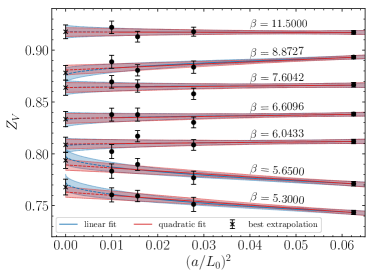
Once inserted in Eq. (7), these results lead to the values of the perturbatively improved definition of shown in Figure 2 for the values of considered. Due to the O()-improvement of the expectation values of the flavour-singlet vector current, we expect that the leading lattice artifacts of are quadratic with terms of the form , and . The last ones are part of the definition of which, as usual, depends on the correlators used to fix it. Their contribution vanishes proportionally to when renormalized matrix elements are extrapolated to the continuum limit. The first two terms are, instead, relevant when taking the limit at fixed lattice spacing. In particular, there can be linear terms in but, due to the multiplicative factor , their relevance decreases with respect to the quadratic ones as the lattice spacing becomes smaller. Our numerical data for show a very weak dependence on and both the linear and the quadratic fits provide practically equivalent extrapolations in within error bars with /d.o.f. close to 1 or smaller: they are displyed in Figure 2 by shaded bands. Taking a conservative approach, we consider the average of the two extrapolations as our best estimate for and the largest error bar as an estimate of the uncertainty. Their values are listed in Table 2. Notice that the difference between the extrapolated values and those at is of the order of the statistical error, and always smaller than twice it. As expected from the perturbative results, the feature of having small corrections because of shifted boundary conditions is confirmed also non-perturbatively.
| 5.3000 | 0.768(7) |
| 5.6500 | 0.794(7) |
| 6.0433 | 0.809(7) |
| 6.6096 | 0.833(7) |
| 7.6042 | 0.864(7) |
| 8.8727 | 0.878(7) |
| 11.500 | 0.918(6) |
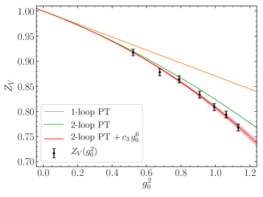
In Figure 3 we plot our final non-perturbative results for at the values of the bare gauge coupling that we have considered, and we compare them with the 1-loop and the 2-loop perturbative expressions [25, 26]: the latter works well up to or so within an accuracy of about 1%. The continuous red band in the Figure is our best fit of the numerical data to the function
| (10) |
where we enforce the value of the coefficients and to be the 1-loop and 2-loop results [25, 26], while the coefficient of the additional term is fitted to describe the mild bending of the data at larger values of the gauge coupling. As a result from Eq. (8) by inserting , from Ref. [26], and from the fit (/d.o.f.=0.31).
4 Conclusions and outlook
Thermal QCD in the presence of non-trivial boundary conditions in the compact direction is the basis for a very effective renormalization strategy for computing renormalization constants of what become conserved charges in the continuum limit. They can be computed by considering 1-point functions, a fact that reduces drastically the numerical effort needed.
Here we have explored in detail this possibility computing the renormalization constant of the QCD flavour-singlet local vector current non-perturbatively in the theory with three massless O()-improved Wilson quarks. With a moderate computational cost, we have achieved a final accuracy on of approximatively 8‰ for values of the inverse bare coupling constant in the range . The best parameterization of our results is given in Eq. (10). The comparison with the known 2-loop perturbative formula suggests that our parameterization works well, within the precision quoted, also for larger values of outside the range explored numerically. For or so we observe significant deviations from the 2-loop result. The rather good agreement with the 2-loop formula in the range explored is an indication that either higher perturbative orders or residual discretization effects in the non-perturbative determination are quite small. It is interesting to notice that, although one could consider usual periodic boundary conditions, shifted boundary conditions have turned out to be a very convenient choice for reducing the magnitude of lattice artifacts.
The results reported in this letter represent the first evaluation of a renormalization constant of a composite operator in QCD in this framework. Our findings open the way to a numerically efficient method for the more challenging problem of computing the renormalization constants of the energy-momentum tensor. The experience we have accumulated in this work, the data generated and the parameter tuning can be directly used in that case.
The generalization to operators which are not discretizations of conserved charges in the continuum, instead, require dedicated theoretical investigations to avoid unnecessarily complicated perturbative expansions and/or matching conditions.
Acknowledgement
We wish to thank R. Sommer for interesting correspondence on the subject of this paper. We acknowledge PRACE for awarding us access to the HPC system MareNostrum4 at the Barcelona Supercomputing Center (Proposals n. 2018194651 and 2021240051). We also thank CINECA for providing us with computer-time on Marconi (CINECA-INFN, CINECA-Bicocca agreements). The R&D has been carried out on the PC clusters Wilson and Knuth at Milano-Bicocca. We thank all these institutions for the technical support. Finally we acknowledge partial support by the INFN project “High performance data network”.
Appendix A QCD lattice action
The action of the lattice theory is written as
| (11) |
where and are the gluonic and fermionic contributions respectively. In this study for the gluonic one we consider the Wilson action
| (12) |
where is the bare gauge coupling, is the plaquette field defined by
| (13) |
and indicates the unit vector oriented along the direction . The fermionic part reads
| (14) |
where is the bare quark mass matrix. The O()-improved Wilson-Dirac operator is the sum of the massless Wilson-Dirac operator, , and the Sheikholeslami-Wohlert operator [17], , defined as
| (15) |
where . The covariant lattice derivatives and are defined by
| (16) |
while the clover discretization of the field strength tensor is given by
| (17) |
with
| (18) |
The coefficient is tuned in order to remove O() lattice artifacts generated by the action in on-shell correlation functions [29]. The mass matrix has been fixed to , where is the critical mass as determined in Ref. [29, 31]. More details on the tuning of the parameters can be found in Appendix A and B of Ref. [24].
Appendix B Perturbative computation
In this Appendix we discuss the computation of and at O() in lattice perturbation theory. We present here only the relevant expressions, while for the details of our conventions and notation we refer readers to Ref. [6]: in particular, the results of the calculation for the conserved flavour-singlet vector current can be found in Appendix G of that reference. The computation is carried out in the presence of shifted boundary conditions and of a twist fermion phase for a generic number of colours, , and of quark flavours, . We write the expectation value of the local current as follows
| (19) |
where the tree-level value is given by
| (20) |
The definitions of the integrals , and of similar ones that appear below can be found at the end of this Appendix. The O() contribution can be written as the sum of three terms,
| (21) |
whose expressions are
| (22) |
| (23) | |||
| (24) |
and we have defined .
The Sheikholeslami-Wohlert term for the O()-improvement of the action adds two contributions to the O() coefficient,
| (25) |
which are given by
| (26) | |||
| (27) | |||
At O() the critical mass reads
| (28) |
where and
| (29) |
with [32]
| (30) | |||
The O() term in the critical mass generates an extra contribution to the expectation value of the vector current which reads
| (31) |
where
| (32) |
We list here the definitions of the tree-level fermionic integrals we have introduced above
| (33) |
| (34) |
together with the bosonic one .
Based on the above results and those discussed in Ref. [6] for the conserved vector current, we have computed the perturbative expansion of at O() in infinite spatial volume. The results can be written as
where
| (36) |
In Eqs. (B) and (36), the coefficients , , , depend on the extension of the compact direction because of discretization effects. Their numerical values at with shift are collected in Table 3 for several values of . These are the coefficients to be used in Eq. (7) to improve the non-perturbative results presented in Section 3. The values in the Table 3 suggest also that, at least at this order in perturbation theory, discretization errors for are tiny for the larger temporal extensions.
| 4 | 1.112904 | -0.071406 | 0.012116 | 0.001336 |
|---|---|---|---|---|
| 6 | 1.021530 | -0.067500 | 0.014571 | 0.001616 |
| 8 | 1.005285 | -0.066005 | 0.015062 | 0.001689 |
| 10 | 1.001882 | -0.065592 | 0.015097 | 0.001708 |
References
- Lüscher, Martin and Narayanan, Rajamani and Weisz, Peter and Wolff, Ulli [1992] Lüscher, Martin and Narayanan, Rajamani and Weisz, Peter and Wolff, Ulli, Nucl. Phys. B 384 (1992) 168–228. doi:10.1016/0550-3213(92)90466-O. arXiv:hep-lat/9207009.
- Martinelli et al. [1995] G. Martinelli, C. Pittori, C. T. Sachrajda, M. Testa, A. Vladikas, Nucl. Phys. B 445 (1995) 81--108. doi:10.1016/0550-3213(95)00126-D. arXiv:hep-lat/9411010.
- Lüscher [2010] M. Lüscher, JHEP 08 (2010) 071. doi:10.1007/JHEP08(2010)071. arXiv:1006.4518, [Erratum: JHEP 03, 092 (2014)].
- Giusti and Meyer [2013] L. Giusti, H. B. Meyer, JHEP 01 (2013) 140. doi:10.1007/JHEP01(2013)140. arXiv:1211.6669.
- Giusti and Pepe [2015] L. Giusti, M. Pepe, Phys. Rev. D 91 (2015) 114504. doi:10.1103/PhysRevD.91.114504. arXiv:1503.07042.
- Dalla Brida et al. [2020] M. Dalla Brida, L. Giusti, M. Pepe, JHEP 04 (2020) 043. doi:10.1007/JHEP04(2020)043. arXiv:2002.06897.
- Giusti and Meyer [2011a] L. Giusti, H. B. Meyer, Phys. Rev. Lett. 106 (2011a) 131601. doi:10.1103/PhysRevLett.106.131601. arXiv:1011.2727.
- Giusti and Meyer [2011b] L. Giusti, H. B. Meyer, JHEP 11 (2011b) 087. doi:10.1007/JHEP11(2011)087. arXiv:1110.3136.
- Hatton et al. [2020] D. Hatton, C. T. H. Davies, G. P. Lepage, A. T. Lytle (HPQCD), Phys. Rev. D 102 (2020) 094509. doi:10.1103/PhysRevD.102.094509. arXiv:2008.02024.
- Green et al. [2017] J. Green, N. Hasan, S. Meinel, M. Engelhardt, S. Krieg, J. Laeuchli, J. Negele, K. Orginos, A. Pochinsky, S. Syritsyn, Phys. Rev. D 95 (2017) 114502. doi:10.1103/PhysRevD.95.114502. arXiv:1703.06703.
- Bochicchio et al. [1985] M. Bochicchio, L. Maiani, G. Martinelli, G. C. Rossi, M. Testa, Nucl. Phys. B 262 (1985) 331. doi:10.1016/0550-3213(85)90290-1.
- Martinelli et al. [1991] G. Martinelli, C. T. Sachrajda, A. Vladikas, Nucl. Phys. B 358 (1991) 212--227. doi:10.1016/0550-3213(91)90538-9.
- Dalla Brida et al. [2019] M. Dalla Brida, T. Korzec, S. Sint, P. Vilaseca, Eur. Phys. J. C 79 (2019) 23. doi:10.1140/epjc/s10052-018-6514-5. arXiv:1808.09236.
- Gerardin et al. [2019] A. Gerardin, T. Harris, H. B. Meyer, Phys. Rev. D 99 (2019) 014519. doi:10.1103/PhysRevD.99.014519. arXiv:1811.08209.
- Heitger and Joswig [2021] J. Heitger, F. Joswig (ALPHA), Eur. Phys. J. C 81 (2021) 254. doi:10.1140/epjc/s10052-021-09037-4. arXiv:2010.09539.
- Blum [2003] T. Blum, Phys. Rev. Lett. 91 (2003) 052001. doi:10.1103/PhysRevLett.91.052001. arXiv:hep-lat/0212018.
- Sheikholeslami and Wohlert [1985] B. Sheikholeslami, R. Wohlert, Nucl. Phys. B 259 (1985) 572. doi:10.1016/0550-3213(85)90002-1.
- Hasenfratz and Karsch [1983] P. Hasenfratz, F. Karsch, Phys. Lett. B 125 (1983) 308--310. doi:10.1016/0370-2693(83)91290-X.
- Roberge and Weiss [1986] A. Roberge, N. Weiss, Nucl. Phys. B 275 (1986) 734--745. doi:10.1016/0550-3213(86)90582-1.
- Gérardin et al. [2018] A. Gérardin, J. Green, O. Gryniuk, G. von Hippel, H. B. Meyer, V. Pascalutsa, H. Wittig, Phys. Rev. D 98 (2018) 074501. doi:10.1103/PhysRevD.98.074501. arXiv:1712.00421.
- Bhattacharya et al. [2006] T. Bhattacharya, R. Gupta, W. Lee, S. R. Sharpe, J. M. S. Wu, Phys. Rev. D 73 (2006) 034504. doi:10.1103/PhysRevD.73.034504. arXiv:hep-lat/0511014.
- Giusti and Pepe [2014] L. Giusti, M. Pepe, Phys. Rev. Lett. 113 (2014) 031601. doi:10.1103/PhysRevLett.113.031601. arXiv:1403.0360.
- Giusti and Pepe [2017] L. Giusti, M. Pepe, Phys. Lett. B 769 (2017) 385--390. doi:10.1016/j.physletb.2017.04.001. arXiv:1612.00265.
- Dalla Brida et al. [2021] M. Dalla Brida, L. Giusti, T. Harris, D. Laudicina, M. Pepe (2021). arXiv:2112.05427.
- Gabrielli et al. [1991] E. Gabrielli, G. Martinelli, C. Pittori, G. Heatlie, C. T. Sachrajda, Nucl. Phys. B 362 (1991) 475--486. doi:10.1016/0550-3213(91)90569-J.
- Skouroupathis and Panagopoulos [2009] A. Skouroupathis, H. Panagopoulos, Phys. Rev. D 79 (2009) 094508. doi:10.1103/PhysRevD.79.094508. arXiv:0811.4264.
- Wohlert [1987] R. Wohlert, DESY preprint 87-069, unpublished (1987).
- Lüscher, M. and Weisz, P. [1996] Lüscher, M. and Weisz, P., Nucl. Phys. B 479 (1996) 429--458. doi:10.1016/0550-3213(96)00448-8. arXiv:hep-lat/9606016.
- Yamada et al. [2005] N. Yamada, et al. (JLQCD, CP-PACS), Phys. Rev. D 71 (2005) 054505. doi:10.1103/PhysRevD.71.054505. arXiv:hep-lat/0406028.
- Collaboration [2021] ALPHA. Collaboration, internal notes ALPHA Collaboration, in preparation for publication (2021).
- Dalla Brida et al. [2018] M. Dalla Brida, P. Fritzsch, T. Korzec, A. Ramos, S. Sint, R. Sommer (ALPHA), Eur. Phys. J. C 78 (2018) 372. doi:10.1140/epjc/s10052-018-5838-5. arXiv:1803.10230.
- Panagopoulos and Proestos [2002] H. Panagopoulos, Y. Proestos, Phys. Rev. D65 (2002) 014511. doi:10.1103/PhysRevD.65.014511. arXiv:hep-lat/0108021.