Time spent in a ball by a critical branching random walk

Abstract

We study a critical branching random walk on $\mathbb{Z}^{d}$. We focus on the tail of the time spent in a ball, and our study, in dimension four and higher, sheds new light on the recent result of Angel, Hutchcroft and Jarai [AHJ21], in particular on the special features of the critical dimension four. Finally, we analyse the number of walks transported by the branching random walk on the boundary of a distant ball.

Keywords and phrases. Branching random walk; local times; range.
MSC 2010 subject classifications. Primary 60G50; 60J80.

1 Introduction

In this paper we study a critical branching random walk (BRW) on $\mathbb{Z}^{d}$. Whereas the study of the volume of the range of random walks is a central object of probability theory, the range of branching random walks, in dimension larger than one, stayed in the shadows. Quite recently, Le Gall and Lin [LGL15, LGL16] proved limit theorems for the volume of the range, say $\mathcal{R}_{n}$, of a random walk indexed by a Galton-Watson tree conditioned on having $n$ vertices, as $n$ goes to infinity. In particular they discovered that in dimension five and larger, $\mathcal{R}_{n}$ scales linearly, whereas in dimension four it scales like $n/\log(n)$, and in dimension three and lower it scales like $n^{d/4}$. Thus with BRW one recovers the well-known trichotomy for the asymptotic behavior of the range of a simple random walk, going back to Dvoretzky and Erdös [DE51], except that the critical dimension is now equal to four instead of two. Later, Zhu in a series of works [Zhu16a, Zhu16b, Zhu19, Zhu21] extended part of Le Gall and Lin’s analysis to general offspring and jump distributions, and most notably brought into light the notion of branching capacity, which is associated with BRW just as the electrostatic capacity is associated with random walk. Lalley and Zheng [LZ11], analyzed the occupation statistics at a fixed generation of the tree, and observed similar behaviors as for a simple random walk. Angel, Hutchcroft and Jarai in [AHJ21] studied the tail of the local times for the full tree, and discovered that the tail speed is exponential in upper critical dimensions (five and higher), but stretched exponential in the critical dimension four, a fact which does not have natural counterpart in the random walk setting. One of our motivation for the present paper is to bring some light on this remarkable observation, and in particular explain the tail behaviour in dimensions four and higher. When [AHJ21] follows a moment method, rooted in statistical mechanics, our approach is probabilistic, and aims at developing an analogue of excursion theory so useful to analyse random walks. Finally, to emphasize the recent vigor of BRW studies in high dimensions, let us mention [BC12] dealing with recurrence of a discrete snake up to dimension four, some recent results on the electrostatic capacity of the range of a BRW [BW20, BH21, BH22], and others on Branching interlacements [PZ19, Zhu18], or on the range of tree-valued BRWs [DKLT].

One important issue going back to Donsker-Varadhan [DV75] is to understand how a random walk squeezes its range, and there again the concept of capacity comes into play. Let us recall that if $\Lambda\subset\mathbb{Z}^{d}$, and $H^{+}_{\Lambda}$ is the return time of $\Lambda$ by a transient random walk of law $\mathbf{P}_{x}$ (when its starting point is $x$), then

$$\text{cap}(\Lambda)=\sum_{x\in\Lambda}\mathbf{P}_{x}\big{(}H^{+}_{\Lambda}=\infty\big{)}.$$ (1.1)

To illustrate the role of capacity in the downward deviation of the range, and explain our present motivation, we recall a key tool obtained in [AS20b]. Assume $d\geq 3$, and let us introduce some notation: given $r>0$ and $x\in\mathbb{Z}^{d}$, we denote by $x+B_{r}$ the Euclidean ball of radius $r$ and center $x\in\mathbb{Z}^{d}$, and let $\ell_{\infty}(x+B_{r})$ be the time spent by a simple random walk on $x+B_{r}$. Then given $\mathcal{C}\subset\mathbb{Z}^{d}$ finite and $\rho$ such that $\rho\cdot r^{d-2}$ is larger than some universal constant, one has for some constant $\kappa>0$,

$$\sup_{z\in\mathbb{Z}^{d}}\mathbf{P}_{z}\big{(}\ell_{\infty}(x+B_{r})\geq\rho\cdot r^{d},\ \forall x\in\mathcal{C}\big{)}\leq\exp\Big{(}-\kappa\cdot\rho\cdot\text{cap}\big{(}\cup_{x\in\mathcal{C}}(x+B_{r})\big{)}\Big{)}.$$ (1.2)

The analogous inequality for branching random, with the capacity replaced by the branching capacity, seems yet a challenging problem at the moment. This would pave the way to studying downward deviations of the range of a BRW in dimension five and larger. Dimension four, as we explain later is special, and we believe that the intuition and concepts built from studying random walks will need to be further expanded.

Here, we consider one Euclidean ball centered at the origin, and study two objects: (i) the tail of the time spent in this ball when the BRW starts at the origin; (ii) the tail of the (rescaled) number of walks hitting the ball, when the BRW starts from far away.

To state our results, let us introduce the needed notation. We let $\mathbf{\mathcal{T}}$ be a critical Bienaymé-Galton-Watson tree (BGW tree for short), whose offspring distribution has a finite exponential moment. Consider $\{S_{u},u\in\mathbf{\mathcal{T}}\}$ an associated tree-indexed random walk, which we view alternatively as a branching random walk, where time is encoded by the tree $\mathcal{T}$ and whose jump distribution is centered, non-degenerate and supported on the set of neighbors of the origin. In other words, independent increments $\{X(e)\}$ are associated to the edges of the tree, and if $[\varnothing,u]$ is the sequence of edges between the root $\varnothing$ and vertex $u$, then

$$S_{u}=S_{\varnothing}+\sum_{e\in[\varnothing,u]}X(e).$$

When $z\in\mathbb{Z}^{d}$, we let $\mathbb{P}_{z}$ be the law of the BRW starting from $z$, i.e. conditioned on $\{S_{\varnothing}=z\}$, and simply write $\mathbb{P}$ when it starts from the origin. Given $\Lambda\subset\mathbb{Z}^{d}$, we define the time spent in $\Lambda$ by the BRW as

$$\ell_{\mathcal{T}}(\Lambda):=\sum_{u\in\mathcal{T}}{\text{\Large$\mathfrak{1}$}}\{S_{u}\in\Lambda\}.$$ (1.3)

Let $B_{r}:=\{z\in\mathbb{Z}^{d}:\|z\|<r\}$, where $\|\cdot\|$ denotes the Euclidean distance, and write $\Theta(f(t,r))$ for a function which is uniformly bounded from above and below by $f$, up to universal multiplicative positive constants. Our main result reads as follows.

Theorem 1.1.

One has uniformly in $r\geq 1$, and $t\geq 1$,

$$\mathbb{P}(\ell_{\mathcal{T}}(B_{r})>t)=\Theta\Big{(}\frac{1}{\sqrt{\min(t,r^{4})}}\Big{)}\times\left\{\begin{array}[]{ll}\exp\Big{(}-\Theta(t/r^{4})\Big{)}&\text{if }d\geq 5\\ \exp\Big{(}-\Theta(\sqrt{t/r^{4}})\Big{)}&\text{if }d=4\\ (1+\frac{t}{r^{4}})^{-\frac{2}{4-d}}&\text{if }d=1,2,3.\\ \end{array}\right.$$ (1.4)

Remark 1.2.

In fact the result in dimension $1$ and $2$ holds under the weaker assumption that the offspring distribution of the BGW tree has only a finite second moment, and a finite third moment in dimension three, instead of a finite exponential moment. Moreover, the proof in dimension $1,2,3$ can be done the same way as in [AHJ21], using a simple moment method. However, in higher dimension, it is unclear how to extend their method in order to extract the scaling of time in $r^{4}$. On the other hand, our hypothesis on the jump distribution could aslo be weakend. For instance assuming that it has finite support would be fine.

Heuristics.

Let us explain at a heuristic level the difference between dimension four on one hand and five and higher on the other hand. In the latter case, to occupy $B_{r}$, a good strategy for the BRW is to produce waves, which go from the boundary $\partial B_{r}$, up to the boundary of a larger concentric ball, say $\partial B_{2r}$, and back to $B_{r}$. Furthermore, (i) each wave starting with order $r^{2}$ BRWs hits the other boundary with order $r^{2}$ particles, at a constant cost; and (ii) when a single BRW starts on $\partial B_{r}$, it spends typically a time $r^{2}$ in $B_{r}$. Thus $t/r^{4}$ waves typically produce a local time $t$ in $B_{r}$, and the cost is that of creating these $t/r^{4}$ waves.

In dimension four, the situation is drastically different: conditioned on coming from a distance $R$, a BRW typically brings $r^{2}\cdot\log(R/r)$ on the boundary of $B_{r}$, so there is some advantage of coming from far away (the $\log(R/r)$ factor is absent in $d\geq 5$). This can be seen by saying that the process conditioned on hitting $B_{r}$ has a single spine from which critical BRWs grow. We show that a correct scenario (see Figure  2 in Section 10) consists in producing $\log(R/r)$ spines, bringing a total number of particles of order $r^{2}\cdot\log^{2}(R/r)$ and we equate this order with $t/r^{2}$ to get the desired stretched exponential cost.

Theorem 1.1 generalizes the analysis of [AHJ21], and its proof follows a probabilistic method. In this proof, we encounter many interesting objects whose exponential moments are studied, and they do present interest on their own. In order to present these additional results, we now define more objects. For a subset $\Lambda\subset\mathbb{Z}^{d}$, let $\mathcal{T}(\Lambda)$ be the set of vertices of $\mathcal{T}$ at which the BRW is in $\Lambda$, as well as at all its ancestral positions. In other words,

$$\mathbf{\mathcal{T}}(\Lambda):=\big{\{}u\in\mathbf{\mathcal{T}}:S_{v}\in\Lambda,\text{ for all }v\leq u\},$$ (1.5)

where we write $v\leq u$ if $v$ is an ancestor of $u$ (by which we include the case $v=u$). Also, the set of vertices corresponding to hitting times of $\Lambda$ is denoted as

$$\eta(\Lambda):=\big{\{}u\in\mathbf{\mathcal{T}}:S_{u}\in\Lambda\text{ and }S_{v}\notin\Lambda\text{ for all }v<u\},$$ (1.6)

where by $v<u$ we mean that $v$ is an ancestor of $u$, which is different from $u$. Our main new estimates concern the exponential moments of the number of frozen particles during each wave. There are two distinct problems as whether we deal with starting points inside the ball, or outside it; the latter problem being the technical core of this paper.

Our first result concerns the case of a starting point lying inside the ball $B_{r}$, and we freeze walks as they reach its outer boundary $\partial B_{r}$. The result holds true irrespective of the dimension. For simplicity we write $\eta_{r}:=\eta(\partial B_{r})$.

Theorem 1.3.

Assume $d\geq 1$. There exist positive constants $c$ and $\lambda_{0}$ (only depending on the dimension), such that for any $0\leq\lambda\leq\lambda_{0}$, and any $r\geq 1$,

$$\sup_{x\in B_{r}}\,\mathbb{E}_{x}\Big{[}\exp(\lambda\frac{|\eta_{r}|}{r^{2}})\Big{]}\leq\exp(\frac{c\lambda}{r^{2}}).$$ (1.7)

Moreover,

$$\sup_{x\in B_{r}}\,\mathbb{E}_{x}\Big{[}\exp(\lambda\frac{|\eta_{r}|}{r^{2}})\ \big{|}\ \eta_{r}\neq\varnothing\Big{]}\leq\exp(c\lambda),$$ (1.8)

and

$$\sup_{x\in B_{r/2}}\,\mathbb{E}_{x}\Big{[}\exp(\lambda\frac{|\eta_{r}|}{r^{2}})\Big{]}\leq\exp\big{(}\frac{\lambda+c\lambda^{2}}{r^{2}}\big{)}.$$ (1.9)

Actually (1.8) easily follows from (1.7), once we know that the probability for the BRW to exit $B_{r}$ starting from a point inside $B_{r}$, is at least of order $1/r^{2}$, see Lemma 3.7. On the other hand, (1.9) follows from (1.8), once we know that the former probability, starting from a point in $B_{r/2}$ is at most of order $1/r^{2}$, see Proposition 3.10.

Thus the heart of the matter is to prove (1.7). For this, we first show an analogous estimate for the total time spent inside the ball $B_{r}$ by a BRW killed on its boundary, whose set of particles is given by $\mathcal{T}(B_{r})$, see (1.5) and Proposition 1.4 below. Then we observe that $|\eta_{r}|$ and $|\mathcal{T}(B_{r})|$ are linked via some natural martingales whose exponential moments are controlled by those of $|\mathcal{T}(B_{r})|$.

Proposition 1.4.

Assume $d\geq 1$. There exist positive constants $c$ and $\lambda_{0}$, such that for any $0\leq\lambda\leq\lambda_{0}$, and any $r\geq 1$,

$$\sup_{x\in B_{r}}\ \mathbb{E}_{x}\Big{[}\exp\big{(}\lambda\frac{|\mathbf{\mathcal{T}}(B_{r})|}{r^{4}}\big{)}\Big{]}\leq\exp(c\frac{\lambda}{r^{2}}).$$

In fact we prove a slightly stronger result in Proposition 9.1, which provides an important additional factor $1/r^{2}$ in the tail distribution, needed in the proof of Theorem 1.1.

To conclude the proof of Theorem 1.1, we need to control the exponential moments of $|\eta_{r}|$, when starting from a point outside $B_{r}$. This part is delicate, and this is where the role of the dimension comes into play. Roughly, the reason for this is that it could happen that many particles would freeze on $\partial B_{r}$, only after doing very large excursions away from it. In dimension five and higher the price to pay for these large excursions is too expensive for playing a significative role. As a consequence one can deduce a result which is similar to Theorem 1.3. Let us however emphasize the factor $(1-\varepsilon)$ appearing in (1.12), which comes from the transience of the random walk in dimension three and higher, and which guarantees that only a finite number of waves matter.

Theorem 1.5.

Assume $d\geq 5$. There exist positive constants $c$ and $\lambda_{0}$ (only depending on the dimension), such that for any $0\leq\lambda\leq\lambda_{0}$, any $r\geq 1$, and $x\in B_{2r}^{c}$,

$$\mathbb{E}_{x}\Big{[}\exp(\lambda\frac{|\eta_{r}|}{r^{2}})\Big{]}\leq\exp(\frac{c\lambda}{\|x\|^{2}}).$$ (1.10)

As a consequence,

$$\sup_{x\in\partial B_{2r}}\mathbb{E}_{x}\Big{[}\exp(\lambda\frac{|\eta_{r}|}{r^{2}})\ \Big{|}\ \eta_{r}\neq\varnothing\Big{]}\leq\exp(c\lambda),$$ (1.11)

and there exists $\varepsilon\in(0,1)$, such that for any $r\geq 1$, and any $0\leq\lambda\leq\lambda_{0}$,

$$\sup_{x\in\partial B_{2r}}\mathbb{E}_{x}\left[\exp\big{(}\lambda\frac{|\eta_{r}|}{r^{2}}\big{)}\right]\leq\exp\big{(}\frac{\lambda(1-\varepsilon)}{r^{2}}\big{)}.$$ (1.12)

In dimension four on the other hand, things are more subtle, and large excursions start to play a decisive role. In particular, one can show that all exponential moments of $|\eta_{r}|/r^{2}$ are infinite, when starting for instance from $\partial B_{2r}$. Thus one needs to consider instead a truncated version of $\eta_{r}$ and renormalize it conveniently. We do this here, by killing the BRW once it reaches some large distance. To formulate our result, we define the deposition on $B_{r}$ of trajectories which remain in $B_{R}$ for $R>2r$:

$$\eta_{r,R}=\eta_{r}\cap\mathcal{T}(B_{R}).$$ (1.13)

In other words $\eta_{r,R}$ is the set of vertices of $\mathcal{T}(B_{R})$ corresponding to hitting times of $\partial B_{r}$. Then, we obtain the following.

Theorem 1.6.

Assume $d=4$. There exist positive constants $c$ and $\lambda_{0}$, such that for any $0\leq\lambda\leq\lambda_{0}$, any $r\geq 1$, $R\geq 2r$, and all $x\in B_{R}\setminus B_{2r}$,

$$\mathbb{E}_{x}\Big{[}\exp\big{(}\frac{\lambda|\eta_{r,R}|}{r^{2}\log(R/r)}\big{)}\Big{]}\leq\exp\big{(}\frac{c\lambda}{\|x\|^{2}\log(R/r)}\big{)}.$$ (1.14)

Furthermore,

$$\sup_{x\in\partial B_{2r}}\mathbb{E}_{x}\Big{[}\exp\big{(}\frac{\lambda|\eta_{r,R}|}{r^{2}\log(R/r)}\big{)}\ \Big{|}\ \eta_{r,R}\neq\varnothing\Big{]}\leq\exp(c\lambda),$$ (1.15)

and there exists $\varepsilon\in(0,1)$, such that

$$\sup_{x\in\partial B_{2r}}\mathbb{E}_{x}\left[\exp\big{(}\frac{\lambda|\eta_{r,R}|}{r^{2}\log(R/r)}\big{)}\right]\leq\exp\big{(}\frac{\lambda(1-\varepsilon)}{r^{2}\log(R/r)}\big{)}.$$ (1.16)

These estimates allow to consider starting points which are not contained in the ball (equivalently balls not centered at the origin). For instance when $d\geq 5$, then uniformly in $r\geq 1$, $t\geq 1$, and $\|x\|\geq 2r$,

$$\mathbb{P}_{x}(\ell_{\mathcal{T}}(B_{r})>t)=\Theta\big{(}\frac{r^{d-4}}{\|x\|^{d-2}}\big{)}\times\exp\big{(}-\Theta(t/r^{4})\big{)}.$$

Similar estimates could be proved when $\|x\|\leq 2r$, depending on the value of $t$, and the same could also be done in lower dimension.

The rest of the paper is organized as follows. Section 2 sets the notation and recall some basic results. Section 3 deals with some moment bounds for a Bienaymé-Galton-Watson process. We also recall there the spine decomposition of the BRW obtained by Zhu, and give bounds for the small moments of $|\eta_{r}|$ both when the starting point lies inside and outside the ball. Section 4 deals with Theorem 1.1 in low dimensions, and Section 5 deals with the exponential moments of the size of the localized BRW, as presented in Proposition 1.4. Theorem 1.3 is proved in Section 6. The technical heart of the paper spreads over three sections: Theorem 1.5 dealing with $d\geq 5$ is proved in Section 7, Theorem 1.6 dealing with $d=4$ is proved in Section 8, and the conclusion of the proof of the upper bounds in Theorem 1.1 for $d\geq 4$ is explained in Section 9. Finally, the lower bounds in high dimensions are given in Section 10.

2 Notation and basic tools

We let $\mathbf{\mathcal{T}}$ be a Bienaymé-Galton-Watson tree (BGW for short), with offspring distribution some measure $\mu$ on the set of integers. Throughout the paper we assume that $\mu$ is critical, in the sense that its mean is equal to one, and that it has a finite variance, which we denote by $\sigma^{2}$. When dimension is three, we assume furthermore that it has a finite third moment, and in higher dimension we assume that it has some finite exponential moment. For $u\in\mathbf{\mathcal{T}}$ we let $\xi_{u}$ be its number of children, so that

$$\mathbb{E}[\xi_{u}]=1,\quad\mathbb{V}\text{ar}(\xi_{u})=\sigma^{2},\quad\text{for all }u\in\mathbf{\mathcal{T}}.$$

We denote the root of the tree by $\varnothing$. We write $|u|$ the generation of a vertex $u\in\mathcal{T}$, i.e. its distance to the root of the tree. We let $u\wedge v$ be the least common ancestor of $u$ and $v$, i.e. the vertex at maximal distance from the root, among the ancestors of both $u$ and $v$. For $n\geq 0$, we let $Z_{n}$ be the number of vertices at generation $n$; in particular by definition $Z_{0}=1$ (the process $\{Z_{n}\}_{n\geq 0}$ is often called a BGW process, or sometimes just a Galton–Watson process in the literature). We also let $\mathcal{T}_{n}:=\{u\in\mathcal{T}:|u|\leq n\}$. It follows from our hypotheses on $\mu$, that for any $n\geq 1$, one has

$$\mathbb{E}[Z_{n}]=1,\quad\text{and}\quad\mathbb{V}\text{ar}(Z_{n})=n\sigma^{2}.$$ (2.1)

We also recall Kolmogorov’s estimate (see [AN72, Theorem 1 p.19]):

$$\mathbb{P}(Z_{n}\neq 0)\sim\frac{2}{\sigma^{2}n},\quad\text{as }n\to\infty.$$ (2.2)

Recall the definition (1.5) of $\mathcal{T}(\Lambda)$, for $\Lambda\subset\mathbb{Z}^{d}$, and for $n\geq 1$, set

$$\mathcal{Z}_{n}(\Lambda)=\{u\in\mathcal{T}(\Lambda):\ |u|=n\}.$$ (2.3)

We define the outer boundary of a subset $\Lambda\subset\mathbb{Z}^{d}$ as

$$\partial\Lambda:=\{z\in\Lambda^{c}:\exists y\in\Lambda\text{ with }\|y-z\|=1\}.$$

We consider $\theta$ some distribution on $\mathbb{Z}^{d}$, which we assume to be centered, supported on the set of neighbors of the origin, and non-degenerate (in the sense that its support really contains all neighbors of the origin). We let $(X_{e})_{e}$ be a collection of independent and identically distributed random variables indexed by the edges of the tree, with law $\theta$ (for a formal construction, see for instance [Shi12]). Then we define the branching random walk $\{S_{u},\ u\in\mathbf{\mathcal{T}}\}$, as the tree-indexed random walk with jump distribution $\theta$, which means that for any vertex $u$, $S_{u}-S_{\varnothing}$ is the sum of the random variables $X_{e}$ along the unique geodesic path from $u$ to the root. We write $\mathbb{E}$ the expectation with respect to the BRW. We let $\mathbf{P}$ be the law of the standard random walk (which we shall also abbreviate as SRW) $\{S_{n}\}_{n\geq 0}$ on $\mathbb{Z}^{d}$, starting from the origin, whose jump distribution is $\theta$. For $x\in\mathbb{Z}^{d}$, we let $\mathbf{P}_{x}$ be the law of the SRW starting from $x$. For $r>0$, we denote by $H_{r}$ the hitting time of $\partial B_{r}$, for the SRW:

$$H_{r}:=\inf\{n\geq 0:S_{n}\in\partial B_{r}\}.$$ (2.4)

If $d\geq 3$, we let $G$ be the Green’s function, which is defined for any $z\in\mathbb{Z}^{d}$, by

$$G(z)=\sum_{n=0}^{\infty}\mathbf{P}(S_{n}=z).$$

We recall that under our assumption on $\theta$, there exists a constant $c_{G}>0$ (only depending on the dimension), such that (see Theorem 4.3.1 in [LL10]):

$$G(z)=c_{G}\cdot\|z\|^{2-d}+\mathcal{O}(\|z\|^{-d}).$$ (2.5)

Furthermore, the function $G$ is harmonic on $\mathbb{Z}^{d}\setminus\{0\}$, in the sense that for all $x$ different from the origin, $G(x)=\mathbf{E}_{x}[G(S_{1})]$. As a consequence, using the optional stopping time theorem, we deduce that for some positive constants $c$ and $C$, one has for any $r\geq 1$ and any $x\notin B_{r}$,

$$\frac{cr^{d-2}}{\|x\|^{d-2}}\leq\frac{G(x)}{\sup_{z\in\partial B_{r}}G(z)}\leq\mathbf{P}_{x}(H_{r}<\infty)\leq\frac{G(x)}{\inf_{z\in\partial B_{r}}G(z)}\leq\frac{Cr^{d-2}}{\|x\|^{d-2}}.$$ (2.6)

As in [AHJ21], we shall also make use of Paley-Zygmund’s inequality, which asserts that for any nonnegative random variable $X$ having finite second moment, and for any $\varepsilon\in[0,1)$,

$$\mathbb{P}(X\geq\varepsilon\mathbb{E}[X])\geq\frac{(1-\varepsilon)^{2}\cdot\mathbb{E}[X]^{2}}{\mathbb{E}[X^{2}]}.$$ (2.7)

A usefull variant of (2.7), which comes after a little algebra reads

$$\mathbb{P}\big{(}X\geq\varepsilon\cdot\mathbb{E}[X\mid X\neq 0]\big{)}\geq\frac{(1-\varepsilon)^{2}\cdot\mathbb{E}[X]^{2}}{\mathbb{E}[X^{2}]}.$$ (2.8)

Finally, given two functions $f$ and $g$, we write $f\lesssim g$, if there exists a constant $C>0$, such that $f\leq Cg$, and similarly for $f\gtrsim g$.

3 Preliminary results

3.1 Exponential moments for the BGW process

In this subsection, we prove two elementary facts on the BGW process. Recall that we assume the offspring distribution $\mu$ to have mean one, and some finite exponential moment. Our first result shows that some exponential moment of $Z_{n}/n$ is finite, conditionally on $Z_{n}$ being nonzero (which is also known to converge in law to an exponential random variable with mean one as $n$ goes to infinity, see [AN72, Theorem 2 p.20]).

Lemma 3.1.

There exist $\lambda>0$, such that

$$\sup_{n\geq 1}\ \mathbb{E}\big{[}\exp(\frac{\lambda Z_{n}}{n})\ \big{|}\ Z_{n}\neq 0\big{]}<\infty.$$ (3.1)

Note that the result is not new, and much stronger results are known, see for instance [NV75, NV03], but for reader’s convenience we shall provide a direct and short proof here.

Proof.

Note that by (2.2), there exists $c>0$, such that for all $n\geq 1$,

$$\mathbb{E}\big{[}\exp(\frac{\lambda Z_{n}}{n})\ \big{|}\ Z_{n}\neq 0\big{]} =1+\frac{\mathbb{E}\big{[}\exp(\frac{\lambda Z_{n}}{n})\big{]}-1}{\mathbb{P}(Z_{n}\neq 0)}$$

$$\leq 1+cn\left(\mathbb{E}\big{[}\exp(\frac{\lambda Z_{n}}{n})\big{]}-1\right).$$

Thus it suffices to show that for some positive constants $c$ and $\lambda_{0}$, one has for all $\lambda\leq\lambda_{0}$, and all $n\geq 1$,

$$\varphi_{n}(\lambda):=\mathbb{E}\big{[}\exp(\frac{\lambda Z_{n}}{n})\big{]}\leq\exp\big{(}\frac{\lambda+c\lambda^{2}}{n}\big{)}.$$ (3.2)

We prove this by induction over $n$. Note that the result for $n=1$ follows from the fact that $Z_{1}$ is distributed as $\mu$, which has a finite exponential moment by hypothesis. Indeed, this implies that for some $c_{0}>0$, and all $\lambda$ small enough,

$$\varphi_{1}(\lambda)=\mathbb{E}\big{[}\exp(\lambda Z_{1})\big{]} \leq 1+\lambda+\lambda^{2}\mathbb{E}\big{[}Z_{1}^{2}\exp(\lambda Z_{1})\big{]}\leq 1+\lambda+c_{0}\lambda^{2}\leq\exp(\lambda+c_{0}\lambda^{2}).$$

Now assume that (3.2) holds true for some $n$, and let us show it for $n+1$. Recall that conditionally on $Z_{n}$, $Z_{n+1}$ is distributed as a sum of $Z_{n}$ i.i.d. random variables with the same law as $Z_{1}$. Therefore, plugging the above computation yields

$$\varphi_{n+1}(\lambda)=\mathbb{E}\big{[}\exp(\frac{\lambda Z_{n+1}}{n+1})\big{]}=\mathbb{E}\left[\varphi_{1}(\frac{\lambda}{n+1})^{Z_{n}}\right]\leq\varphi_{n}\Big{(}\frac{\lambda n}{n+1}+c_{0}\frac{\lambda^{2}n}{(n+1)^{2}}\Big{)}.$$

Note that the induction hypothesis reads also as $n\log\varphi_{n}(\lambda)\leq\lambda+c\lambda^{2}$. Then

$$\begin{split}(n+1)\log\varphi_{n+1}(\lambda)&\leq\frac{n+1}{n}\Big{(}\frac{n}{n+1}\lambda+c_{0}\frac{n}{(n+1)^{2}}\lambda^{2}+c\big{(}\frac{\lambda n}{n+1}+c_{0}\frac{\lambda^{2}n}{(n+1)^{2}}\big{)}^{2}\Big{)}\\ &\leq\lambda+\frac{c_{0}}{n+1}\lambda^{2}+c\frac{n}{n+1}\lambda^{2}+2cc_{0}\frac{\lambda^{3}}{n}+cc_{0}^{2}\frac{\lambda^{4}}{n^{2}}\\ &\leq\lambda+c\lambda^{2}-\frac{c-c_{0}}{n+1}\lambda^{2}+2cc_{0}\frac{\lambda^{3}}{n}+cc_{0}^{2}\frac{\lambda^{4}}{n^{2}}.\end{split}$$ (3.3)

Thus if we choose $c=2c_{0}$, and $\lambda$ small enough so that for any $n\geq 1$,

$$4c_{0}\frac{n+1}{n}\lambda+2c_{0}^{2}\frac{n+1}{n^{2}}\lambda^{2}<1,$$

one obtains

$$\varphi_{n+1}(\lambda)\leq\exp(\frac{\lambda+c\lambda^{2}}{n+1}).$$

This establishes the induction step, and concludes the proof of the lemma. ∎

Our second result concerns the exponential moments for the total size of the BGW tree, up to some fixed generation, and is proved along the same lines.

Lemma 3.2.

There exist positive constants $c$ and $\lambda_{0}$, such that for any $0\leq\lambda\leq\lambda_{0}$, and any $n\geq 1$,

$$\mathbb{E}\big{[}\exp(\frac{\lambda|\mathcal{T}_{n}|}{n^{2}})\big{]}\leq\exp(\frac{\lambda+c\lambda^{2}}{n}).$$

Proof.

We prove the result by induction on $n\geq 1$. The case $n=1$ has already been seen in the proof of Lemma 3.1, and only relies on the fact that $Z_{1}$ has a finite exponential moment by assumption. Assume now that it holds for some $n$, and let us prove it for $n+1$. Since conditionally on $Z_{1}$, $|\mathcal{T}_{n+1}|$ is the sum of $Z_{1}$ i.i.d. random variables distributed as $|\mathcal{T}_{n}|$, we deduce from the induction hypothesis, that for some $c$ and $\lambda_{0}$ one has for all $\lambda\leq\lambda_{0}$,

$$\mathbb{E}\Big{[}\exp(\frac{\lambda|\mathcal{T}_{n+1}|}{(n+1)^{2}})\ \big{|}\ Z_{1}\Big{]}\leq\exp\big{(}\frac{\lambda\frac{n}{n+1}+c\lambda^{2}(\frac{n}{n+1})^{3}}{n+1}Z_{1}\big{)}\leq\exp\Big{(}\frac{\lambda+c\lambda^{2}-\frac{\lambda}{n+1}}{n+1}Z_{1}\Big{)}.$$

Integrating now both sides over $Z_{1}$, and using the result for $n=1$, gives

$$\mathbb{E}\Big{[}\exp(\frac{\lambda|\mathcal{T}_{n+1}|}{(n+1)^{2}})\Big{]}\leq\exp\Big{(}\frac{\lambda+c\lambda^{2}-\frac{\lambda}{n+1}+\frac{c(\lambda+c\lambda^{2})^{2}}{n+1}+\frac{c\lambda^{2}}{(n+1)^{3}}}{n+1}\Big{)}\leq\exp\Big{(}\frac{\lambda+c\lambda^{2}-\frac{\lambda-2c\lambda^{2}+\mathcal{O}(\lambda^{3})}{n+1}}{n+1}\Big{)},$$

and the right-hand side is well smaller than $\exp(\frac{\lambda+c\lambda^{2}}{n+1})$, provided $\lambda_{0}$ is small enough. This concludes the proofs of the induction step, and of the lemma. ∎

3.2 Spine decomposition for the BRW

We present here a spine decomposition of the BRW conditioned to hit a set, which was introduced by Zhu to derive upper bounds on hitting probabilities, see [Zhu16a, Zhu21]. We shall use it also later for proving the lower bound in Theorem 1.1 in dimension four.

Following the terminology of [Zhu16a, Zhu21], an adjoint BGW tree is a BGW tree in which only the law of the number of children of the root has been modified, and follows the law $\widetilde{\mu}$, given by $\widetilde{\mu}(i):=\sum_{j\geq i+1}\mu(j)$, for $i\geq 0$. The associated tree-indexed random walk is the adjoint BRW. Then we define $k_{\Lambda}(x)$, for $x\in\mathbb{Z}^{d}$, as the probability for an adjoint BRW starting from $x$ to hit $\Lambda$. Now, given an integer $n$ and a path $\gamma:\{0,\dots,n\}\to\mathbb{Z}^{d}$, we define, with $|\gamma|=n$,

$$p_{\Lambda}(\gamma):=\prod_{i=0}^{|\gamma|-1}\theta\big{(}\gamma(i+1)-\gamma(i)\big{)}\cdot\big{(}1-k_{\Lambda}(\gamma(i))\big{)}.$$ (3.4)

In other words, $p_{\Lambda}(\gamma)$ is the probability that a SRW starting from $\gamma(0)$ follows the path $\gamma$ during its first $n$ steps, when it is killed at each step with probability given by the function $k_{\Lambda}$ at its current position.

We next define the probability measures $\{\mu_{\Lambda}^{z}\}_{z\in\Lambda^{c}}$ on the integers by

$$\mu_{\Lambda}^{z}(m):=\sum_{\ell\geq 0}\mu(\ell+m+1)r_{\Lambda}(z)^{\ell}/\big{(}1-k_{\Lambda}(z)\big{)},\quad\text{for all }m\geq 0,$$

where $r_{\Lambda}(z)$ is the probability that a BRW starting from $z$ does not visit $\Lambda$, conditionally on the root having only one child. We call biased BRW starting from $z$, a BRW starting from $z$, conditioned on the number of children of the root having law $\mu_{\Lambda}^{z}$.

Furthermore, a finite path $\gamma$, is said to go from $x$ to $\Lambda$, which we denote as $\gamma:x\to\Lambda$, if for $n=|\gamma|$, $\gamma(n)\in\Lambda$, and $\gamma(i)\notin\Lambda$ for all $i<n$. In other words this simply means that the path $\gamma$ is defined up to its hitting time of $\Lambda$ (note that it includes the possibility that $n=0$ and $\gamma(0)\in\Lambda$). We shall also later write for simplicity $\gamma:x\to y$, when $\Lambda$ is reduced to a single point $y$. Then given $x\in\mathbb{Z}^{d}$, and $\gamma:x\to\Lambda$, we call $\gamma$-biased BRW, the union of $\gamma$, together with for each $i\in\{0,\dots,|\gamma|-1\}$, a biased BRW starting from $\gamma(i)$, independently for each $i$, and starting from $\gamma(n)$ some usual independent BRW .

We are now in position to describe the law of the BRW starting at some $x\in\mathbb{Z}^{d}$, and conditioned on hitting $\Lambda$. For simplicity, we restrict us to the part which intersects $\Lambda$, since this is the only one that is needed here. On the event $\{\ell_{\mathcal{T}}(\Lambda)>0\}$, one defines the first entry vertex, as the smallest vertex $u\in\mathcal{T}$ in the lexicographical order, for which $S_{u}\in\Lambda$. Then, denoting by $\overleftarrow{u}$ the unique geodesic path in the BGW tree going from the root to the vertex $u$, we let $\Gamma=\Gamma(\mathcal{T})$ be the path in $\mathbb{Z}^{d}$, made of the successive positions of the BRW along that path. Thus if $\overleftarrow{u}=(u_{0}=\varnothing,u_{1},\dots,u_{n}=u)$, with $n=|u|$, then

$$\Gamma=\big{(}S_{\varnothing}=x,S_{u_{1}},\dots,S_{u_{n}}\big{)}.$$

Note that by definition $\Gamma$ is a path which goes from $x$ to $\Lambda$ in our terminology. The following result comes from [Zhu21, Proposition 2.4].

Proposition 3.3 ([Zhu21]).

Assume $d\geq 1$. Let $\Lambda\subset\mathbb{Z}^{d}$, and $x\in\mathbb{Z}^{d}$ be given.

1. For any path $\gamma:x\to\Lambda$, one has

   $$\mathbb{P}_{x}(\Gamma=\gamma,\ell_{\mathcal{T}}(\Lambda)>0)=p_{\Lambda}(\gamma).$$ (3.5)

2. Furthermore, conditionally on $\{\Gamma=\gamma,\,\ell_{\mathcal{T}}(\Lambda)>0\}$, the trace of the BRW on $\Lambda$ has the same law as the trace of a $\gamma$-biased BRW.

The product formula (3.4) defining $p_{\Lambda}$ implies that $\Gamma$ satisfies the (strong) Markov property, in the following sense. Given $x\in\mathbb{Z}^{d}$, we define a probability measure $\mathbb{P}_{\Lambda}^{x}$ on the set of paths $\gamma:x\to\Lambda$, by

$$\mathbb{P}_{\Lambda}^{x}(\gamma):=\frac{p_{\Lambda}(\gamma)}{\sum_{\gamma^{\prime}:x\to\Lambda}p_{\Lambda}(\gamma^{\prime})},$$

which is nothing else than the law of $\Gamma$, conditionally on the event $\{\ell_{\mathcal{T}}(\Lambda)>0\}$. Then we can state the Markov property as follows (we only state a particular case, but the same would hold for any stopping time).

Corollary 3.4.

Let $\Lambda\subset A\subset\mathbb{Z}^{d}$, and $x\in\mathbb{Z}^{d}$ be given. Let $\tau_{A}:=\inf\{i\geq 0:\Gamma(i)\in A\}$. Then for any path $\gamma:x\to\Lambda$, one has

$$\mathbb{P}_{\Lambda}^{x}\Big{(}(\Gamma(\tau_{A}),\dots)=\gamma\mid\Gamma(0),\dots,\Gamma(\tau_{A})\Big{)}=\mathbb{P}_{\Lambda}^{\Gamma(\tau_{A})}(\gamma).$$

Proof.

It suffices to notice that by (3.4), for any path $\gamma_{0}:x\to\gamma(0)$, writing $\gamma\circ\gamma_{0}$ for the concatenation of $\gamma_{0}$ and $\gamma$, one has

$$\mathbb{P}_{\Lambda}^{x}\Big{(}(\Gamma(\tau_{A}),\dots)=\gamma\mid(\Gamma(0),\dots,\Gamma(\tau_{A}))=\gamma_{0}\Big{)} =\frac{p_{\Lambda}(\gamma\circ\gamma_{0})}{\sum_{\gamma^{\prime}:x\to\Lambda}p_{\Lambda}(\gamma^{\prime})}\times\frac{\sum_{\gamma^{\prime}:x\to\Lambda}p_{\Lambda}(\gamma^{\prime})}{p_{\Lambda}(\gamma_{0})\sum_{\gamma^{\prime\prime}:\gamma(0)\to\Lambda}p_{\Lambda}(\gamma^{\prime\prime})}$$

$$=\frac{p_{\Lambda}(\gamma)\cdot p_{\Lambda}(\gamma_{0})}{p_{\Lambda}(\gamma_{0})\sum_{\gamma^{\prime\prime}:\gamma(0)\to\Lambda}p_{\Lambda}(\gamma^{\prime\prime})}=\mathbb{P}_{\Lambda}^{\gamma(0)}(\gamma).$$

∎

3.3 Hitting Probability Lower Bounds

Here we derive rough lower bounds for the hitting probabilities of balls, using a second moment method. The result is as follows (recall (1.6)):

Lemma 3.5.

There exists a constant $c>0$ (only depending on the dimension), such that for any $r\geq 1$ and $x\notin B_{r}$,

$$\mathbb{P}_{x}(|\eta_{r}|>0)\geq c\cdot\left\{\begin{array}[]{ll}\frac{r^{d-4}}{\|x\|^{d-2}}&\text{if }d\geq 5\\ \frac{1}{\|x\|^{2}\log(1+\frac{\|x\|}{r})}&\text{if }d=4.\end{array}\right.$$ (3.6)

Remark 3.6.

Note that in dimension five and higher the result follows from [Zhu16a], which proves as well an upper bound of the same order. We include a short proof here, for the reader’s convenience. In dimension four, a more precise asymptotic is proved in [Zhu21] in case $r=1$ (see also [Zhu19] for a rough upper bound still in the case $r=1$).

Proof.

Recall that we denote by $H_{r}$ the hitting time of $\partial B_{r}$ for a standard random walk. One has, using (2.6) for the last inequality,

$$\mathbb{E}_{x}\big{[}|\eta_{r}|\big{]} =\sum_{n=0}^{\infty}\mathbb{E}_{x}\Big{[}\sum_{|u|=n}{\text{\Large$\mathfrak{1}$}}\{u\in\eta_{r}\}\Big{]}=\sum_{n=0}^{\infty}\mathbb{E}[Z_{n}]\cdot\mathbf{P}_{x}(H_{r}=n)=\mathbf{P}_{x}(H_{r}<\infty)\gtrsim(\frac{r}{\|x\|})^{d-2}.$$

Now we bound the second moment. Recall that by definition, if $u\in\eta_{r}$, then none of its descendant can be in $\eta_{r}$. Thus summing first over all possible $w\in\mathbf{\mathcal{T}}$ and then integrating over all possible $u\neq v$, with $u\wedge v=w$ (and necessarily both $u$ and $v$ different from $w$), gives (recall the notation (2.3))

$$\mathbb{E}_{x}\big{[}|\eta_{r}|^{2}\big{]} =\mathbf{P}_{x}(H_{r}<\infty)+\sum_{k=0}^{\infty}\mathbb{E}_{x}\Big{[}\sum_{w\in\mathcal{Z}_{k}(\partial B_{r}^{c})}\xi_{w}(\xi_{w}-1)\mathbf{P}_{S_{w}}(H_{r}<\infty)^{2}\Big{]}$$

$$=\mathbf{P}_{x}(H_{r}<\infty)+\sigma^{2}\sum_{k=0}^{\infty}\mathbb{E}_{x}\Big{[}\sum_{w\in\mathcal{Z}_{k}(\partial B_{r}^{c})}\mathbf{P}_{S_{w}}(H_{r}<\infty)^{2}\Big{]}$$

$$\leq\mathbf{P}_{x}(H_{r}<\infty)+\sigma^{2}\sum_{k=0}^{\infty}\mathbb{E}_{x}\Big{[}\sum_{|w|=k}{\text{\Large$\mathfrak{1}$}}\{S_{w}\notin\partial B_{r}\}\cdot\mathbf{P}_{S_{w}}(H_{r}<\infty)^{2}\Big{]}$$

$$\lesssim(\frac{r}{\|x\|})^{d-2}+r^{2(d-2)}\sum_{k=0}^{\infty}\mathbf{E}_{x}\Big{[}\frac{{\text{\Large$\mathfrak{1}$}}\{S_{k}\notin\partial B_{r}\}}{\|S_{k}\|^{2(d-2)}}\Big{]}=(\frac{r}{\|x\|})^{d-2}+r^{2(d-2)}\sum_{z\notin B_{r}}\frac{G(z-x)}{\|z\|^{2(d-2)}}$$

$$\lesssim\left\{\begin{array}[]{ll}\frac{r^{d}}{\|x\|^{d-2}}&\text{if }d\geq 5\\ \frac{r^{4}}{\|x\|^{2}}\cdot\log(1+\frac{\|x\|}{r})&\text{if }d=4.\end{array}\right.$$

The result follows using that by Cauchy-Schwarz inequality,

$$\mathbb{P}_{x}(|\eta_{r}|>0)\geq\frac{\mathbb{E}_{x}\big{[}|\eta_{r}|\big{]}^{2}}{\mathbb{E}_{x}\big{[}|\eta_{r}|^{2}\big{]}}.$$

∎

The next result holds in any dimension.

Lemma 3.7.

Assume $d\geq 1$. There exists a constant $c>0$ (only depending on the dimension), such that for any $r\geq 1$,

$$\inf_{x\in B_{r}}\ \mathbb{P}_{x}(|\eta_{r}|>0)\geq c/r^{2}.$$

Proof.

The proof is similar to the previous lemma. Note first that for any $x\in B_{r}$,

$$\mathbb{E}_{x}[|\eta_{r}|]=\mathbf{P}_{x}(H_{r}<\infty)=1,$$

and as before,

$$\mathbb{E}_{x}\big{[}|\eta_{r}|^{2}\big{]}\leq 1+\sigma^{2}\sum_{k=0}^{\infty}\mathbf{P}_{x}(H_{r}>k)=1+\sigma^{2}\,\mathbf{E}_{x}[H_{r}]\lesssim r^{2}.$$

The result follows. ∎

Finally we state a result concerning the first and third moments of $|\eta_{r}|$, when starting from $\partial B_{2r}$.

Lemma 3.8.

Assume $d\geq 1$.

1. For any $x\in B_{r}^{c}$, one has $\mathbb{E}_{x}\big{[}|\eta_{r}|\big{]}=\mathbf{P}_{x}(H_{r}<\infty)$. In particular, when $d\geq 3$, there exists $\varepsilon>0$, such that for any $r\geq 1$,

   $$\sup_{x\in\partial B_{2r}}\mathbb{E}_{x}\big{[}|\eta_{r}|\big{]}\leq 1-\varepsilon.$$

2. Assume $d\geq 4$. There exists $C>0$, such that for any $r\geq 1$,

   $$\sup_{x\in\partial B_{2r}}\mathbb{E}_{x}\big{[}|\eta_{r}|^{3}\big{]}\leq Cr^{4}.$$

Remark 3.9.

The last point of the lemma can be understood, as we think that when starting from $\partial B_{2r}$, the probability to hit $\partial B_{r}$ is of order $1/r^{2}$, and conditionally on hitting it, the number of frozen particles $|\eta_{r}|$ is typically of order $r^{2}$. This reasoning would apply also to all other moments of fixed order, but the third moment will suffice for our purpose.

Proof.

We start with the first point. The equality $\mathbb{E}_{x}\big{[}|\eta_{r}|\big{]}=\mathbf{P}_{x}(H_{r}<\infty)$ has already been seen in the proof of Lemma 3.5. Then the fact that if $\|x\|\geq 2r$, this quantity is bounded from above by some constant smaller than one, in dimension three and higher, follows from (2.5) and (2.6).

Let us prove the second point now. When we sum over triples, say $(u,v,w)\in\eta_{r}$, we distinguish two cases. Either at least two of them are equal, and we just bound the corresponding sum by three times the second moment of $|\eta_{r}|$, or the three points are distinct. In the latter case, we again distinguish between two possible situations: either, $u\wedge v=u\wedge w$, or $u\wedge v\neq u\wedge w$. In both cases, by summing first over $(u\wedge v)\wedge(u\wedge w)$ yields, for any $x\in\partial B_{2r}$, (recall the notation (2.3)),

$$\mathbb{E}_{x}\big{[}|\eta_{r}|^{3}\big{]} \leq 3\mathbb{E}_{x}\big{[}|\eta_{r}|^{2}\big{]}+\sum_{k=0}^{\infty}\mathbb{E}_{x}\Big{[}\sum_{u\in\mathcal{Z}_{k}((\partial B_{r})^{c})}\xi_{u}(\xi_{u}-1)(\xi_{u}-2)\mathbf{P}_{S_{u}}(H_{r}<\infty)^{3}\Big{]}$$

$$+\sum_{k=0}^{\infty}\mathbb{E}_{x}\Big{[}\sum_{u\in\mathcal{Z}_{k}((\partial B_{r})^{c})}\xi_{u}(\xi_{u}-1)\mathbf{P}_{S_{u}}(H_{r}<\infty)\cdot\mathbb{E}_{S_{u}}\big{[}|\eta_{r}|^{2}\big{]}\Big{]}.$$ (3.7)

Next, using (2.6) we get

$$\sum_{k=0}^{\infty}\mathbb{E}_{x}\Big{[}\sum_{u\in\mathcal{Z}_{k}((\partial B_{r})^{c})}\xi_{u}(\xi_{u}-1)(\xi_{u}-2)\mathbf{P}_{S_{u}}(H_{r}<\infty)^{3}\Big{]}$$

$$\leq Cr^{3(d-2)}\sum_{k=0}^{\infty}\mathbf{E}_{x}\Big{[}\frac{{\text{\Large$\mathfrak{1}$}}\{S_{k}\notin B_{r}\}}{\|S_{k}\|^{3(d-2)}}\Big{]}\leq Cr^{3(d-2)}\sum_{z\notin B_{r}}\frac{G(z-x)}{\|z\|^{3(d-2)}}\leq Cr^{2}.$$

Finally for the last sum in  (3.3), we use the computation from the proof of Lemma 3.5, in particular the fact that the second moment of $|\eta_{r}|$ is $\mathcal{O}(r^{2})$, when starting from $x\notin B_{r}$. This yields the upper bound

$$Cr^{2d-2}\sum_{k=0}^{\infty}\mathbf{E}_{x}\Big{[}\frac{{\text{\Large$\mathfrak{1}$}}\{S_{k}\notin B_{r}\}}{\|S_{k}\|^{2(d-2)}}\log(1+\frac{\|S_{k}\|}{r})\Big{]}\leq Cr^{2d-2}\sum_{z\notin B_{r}}\frac{G(z-x)}{\|z\|^{2(d-2)}}\cdot\log(1+\frac{\|z\|}{r})\leq Cr^{4},$$

concluding the proof of the lemma. ∎

3.4 Hitting probability upper bounds

In this section we provide upper bounds for hitting probabilities of balls, which are of the same order as the lower bounds obtained previously. Such bounds were first derived in [LGL15], under an exponential moment assumption for the offspring distribution $\mu$; and then under milder hypotheses in [Zhu16a].

The first result considers hitting probabilities of balls, starting from inside, and for completeness we provide an alternative simple proof.

Proposition 3.10 ([LGL15, Zhu16a]).

Assume $d\geq 1$. There exists $C>0$, such that for any $r\geq 1$,

$$\sup_{x\in B_{r/2}}\mathbb{P}_{x}(|\eta_{r}|>0)\leq\frac{C}{r^{2}}.$$

Proof.

Assume without loss of generality that $r^{2}$ is an integer. We first write for $x\in B_{r/2}$, using (2.2), that some constant $C>0$,

$$\mathbb{P}_{x}(|\eta_{r}|>0) \leq\sum_{k=0}^{r^{2}}\mathbb{P}_{x}(Z_{k}\neq 0,Z_{k+1}=0,|\eta_{r}|>0)+\mathbb{P}(Z_{r^{2}}\neq 0)$$

$$\leq\sum_{k=0}^{r^{2}}\mathbb{P}_{x}(Z_{k}\neq 0,Z_{k+1}=0,|\eta_{r}|>0)+\frac{C}{r^{2}}.$$

Now fix some $k\leq r^{2}$, and note that conditionally on $Z_{k}$, the probability for $Z_{k+1}$ to be zero is equal to $\mu(0)^{Z_{k}}$. Then by using a first moment bound, and the fact that for any vertex at generation $k$, the probability that the BRW reaches $\partial B_{r}$ along the line of its ancestors is given exactly by the probability for a SRW to reach $\partial B_{r}$, we get for some constant $c>0$,

$$\mathbb{P}_{x}(Z_{k}\neq 0,Z_{k+1}=0,|\eta_{r}|>0) \leq\mathbb{E}\big{[}Z_{k}\mu(0)^{Z_{k}}\big{]}\cdot\mathbf{P}_{x}(H_{r}\leq k)$$

$$\lesssim\mathbb{E}\big{[}Z_{k}\mu(0)^{Z_{k}}\big{]}\cdot\exp(-cr^{2}/k),$$

where the last inequality is well-known. Now using (2.2) again, and the fact that $\mu(0)<1$ (since $\mu$ has mean one), we get for some constant $C>0$,

$$\mathbb{E}\big{[}Z_{k}\mu(0)^{Z_{k}}\big{]}=\sum_{n=0}^{\infty}n\mu(0)^{n}\mathbb{P}(Z_{k}=n)\leq\mathbb{P}(Z_{k}>0)\sum_{n\geq 0}n\mu(0)^{n}\leq\frac{C}{k},$$

and the desired result follows. ∎

The second result concerns hitting probabilities of a ball starting from a point outside from it.

Proposition 3.11 ([LGL15, Zhu16a, Zhu19]).

There exists $C>0$, such that for any $r\geq 1$, and any $x\notin B_{2r}$,

$$\mathbb{P}_{x}(|\eta_{r}|>0)\leq C\cdot\left\{\begin{array}[]{ll}\frac{r^{d-4}}{\|x\|^{d-2}}&\text{if }d\geq 5\\ \frac{1}{\|x\|^{2}\log(\|x\|/r)}&\text{if }d=4.\end{array}\right.$$ (3.8)

Proof.

The result in dimension five is given in [Zhu16a], and the proof in dimension four is identical to the case $r=1$, which is done in [Zhu19]. We leave the details to the reader. ∎

3.5 Proof of Theorem 1.1 in short time.

We deal in this section with $t\leq r^{4}$.

The upper bound.

We use that $\ell_{\mathcal{T}}(B_{r})$ coincides essentially with the total size of the BGW tree $\mathcal{T}$. Indeed, using (2.2) and Markov’s inequality, yields

$$\mathbb{P}(\ell_{\mathcal{T}}(B_{r})>t) \leq\mathbb{P}(|\mathbf{\mathcal{T}}|>t)\leq\mathbb{P}(Z_{\sqrt{t}}\neq 0)+\mathbb{P}(1+Z_{1}+\dots+Z_{\sqrt{t}}>t)$$

$$\lesssim\frac{1}{\sqrt{t}}+\frac{1}{t}\cdot\mathbb{E}[Z_{1}+\dots+Z_{\sqrt{t}}]\lesssim\frac{1}{\sqrt{t}},$$

giving the desired upper bound.

The lower bound.

We divide the proof in two steps. We first show that we can bring of the order of $\sqrt{t}$ particles in $B_{r/2}$ at a cost of order $1/\sqrt{t}$, and then we show that conditionally on this event, the union of the BRWs emanating from these particles are likely to spend a time $t$ in the ball $B_{r}$.

Let us start with the first step. Let $r_{0}:=t^{1/4}/2$. Note that by hypothesis $r_{0}\leq r/2$. By Proposition 3.10, one has for some constant $C>0$,

$$\mathbb{P}(|\eta_{r_{0}}|>0)\leq C/\sqrt{t},$$

and since $\mathbb{E}[|\eta_{r_{0}}|]=1$, we have, for some constant $c>0$,

$$\mathbb{E}\big{[}|\eta_{r_{0}}|\ \big{|}\ |\eta_{r_{0}}|>0\big{]}\geq c\sqrt{t}.$$

Then, by using Paley-Zygmund’s inequality (2.8) (with $\varepsilon=1/2$), and the second moment estimates in the proof of Lemma 3.7, we deduce that for some constant $\rho_{1}>0$,

$$\mathbb{P}(|\eta_{r_{0}}|\geq\rho_{1}\sqrt{t})\geq\frac{\rho_{1}}{\sqrt{t}},$$ (3.9)

concluding the first step.

Now we move to the second step. Let $X:=\sum_{\sqrt{t}/4\leq k\leq{\sqrt{t}}}Z_{k}$. We first claim that for some $c_{0}>0$ (independent of $t$ and $r$) we have

$$\mathbb{P}\big{(}X\geq c_{0}t\big{)}\geq\frac{c_{0}}{\sqrt{t}}.$$ (3.10)

Indeed, observe that $\mathbb{E}[X]\geq\frac{1}{2}\sqrt{t}$, and thus by Kolmogorov’s estimate (2.2), one has for some $c>0$,

$$\mathbb{E}[X\mid X\neq 0]\geq ct.$$

On the other hand, using (2.1), we get

$$\mathbb{E}[X^{2}]\leq\sqrt{t}\cdot\sum_{\sqrt{t}/4\leq i\leq\sqrt{t}}\mathbb{E}[Z_{i}^{2}]\leq t^{3/2},$$

and (3.10) follows using Paley-Zygmund’s inequality (2.8).

Now, define

$$Y=\sum_{\sqrt{t}/4\leq|u|\leq\sqrt{t}}{\text{\Large$\mathfrak{1}$}}\{S_{u}\in B_{r}\}.$$ (3.11)

One has for any $z\in\partial B_{r_{0}}$,

$$\mathbb{E}_{z}[Y\mid\mathbf{\mathcal{T}}]=\sum_{\sqrt{t}/4\leq k\leq\sqrt{t}}Z_{k}\cdot\mathbf{P}_{z}(S_{k}\in B_{r})\geq\delta\cdot X,$$

with

$$\delta:=\inf_{x\in B_{r}}\inf_{k\leq r^{2}}\mathbf{P}_{x}(S_{k}\in B_{r})>0.$$

On the other hand, by definition one has $Y\leq X$, and thus (2.7) gives

$$\mathbb{P}_{z}(Y\geq c_{0}\delta t/2\mid\mathbf{\mathcal{T}})\cdot{\text{\Large$\mathfrak{1}$}}\{X\geq c_{0}t\}\geq\frac{\frac{1}{4}\mathbb{E}_{z}\big{[}Y\mid\mathbf{\mathcal{T}}\big{]}^{2}}{\mathbb{E}_{z}\big{[}Y^{2}\mid\mathbf{\mathcal{T}}\big{]}}\cdot{\text{\Large$\mathfrak{1}$}}\{X\geq c_{0}t\}\geq\frac{\delta^{2}}{4}\cdot{\text{\Large$\mathfrak{1}$}}\{X\geq c_{0}t\}.$$

Note also that by definition $Y\leq\ell_{\mathcal{T}}(B_{r})$. Hence, taking expectation on both sides of the last inequality and plugging (3.10), gives with $\rho_{2}:=c_{0}\delta^{2}/4$,

$$\inf_{z\in\partial B_{r_{0}}}\mathbb{P}_{z}(\ell_{\mathcal{T}}(B_{r})\geq\rho_{2}t)\geq\frac{\rho_{2}}{\sqrt{t}}.$$ (3.12)

To conclude, notice that, as mentioned at the beginning of the proof, the time spent in $B_{r}$ is larger than the time spent by the union of the BRWs emanating from the particles in $\eta_{r_{0}}$ (which by definition are on $\partial B_{r_{0}}$). Hence, denoting by $\mathcal{N}$ a Binomial random variable with number of trials $\lfloor\rho_{1}\sqrt{t}\rfloor$ and probability of success $\frac{\rho_{2}}{\sqrt{t}}$, we get using (3.9) together with (3.12), for some constant $\rho>0$ (independent of $t$ and $r$),

$$\mathbb{P}(\ell_{\mathcal{T}}(B_{r})\geq t)\geq\mathbb{P}(\ell_{\mathcal{T}}(B_{r})\geq t,|\eta_{r_{0}}|\geq\rho_{1}\sqrt{t})\geq\mathbb{P}(\mathcal{N}\geq 1/\rho_{2})\cdot\mathbb{P}(|\eta_{r_{0}}|\geq\rho_{1}\sqrt{t})\geq\frac{\rho}{\sqrt{t}},$$

as wanted.

This concludes the proof of Theorem 1.1 in case $t\leq r^{4}$. $\square$

4 Proof of Theorem 1.1 in low dimension

In dimension one, two and three, the proofs are easier, and only require small moment estimates, which enables us to use the results from [AHJ21]. More precisely, in dimension one and two both the lower and upper bounds only require estimates of the first and second moment, and in dimension three we need an additional third moment. We define for $d\in\{1,2,3\}$,

$$R=(t/r^{d})^{\frac{1}{4-d}},\quad\text{and}\quad N=R^{2}.$$

Recall that one can assume here that $t\geq r^{4}$, in which case it amounts to show that

$$\mathbb{P}(\ell_{\mathcal{T}}(B_{r})>t)=\Theta(R^{-2}).$$

The proof is based on the following result, which is Lemma 4.3 in [AHJ21]. For $n\geq 0$, and $x\in\mathbb{Z}^{d}$, write

$$\ell_{n}(x)=\sum_{|u|\leq n}{\text{\Large$\mathfrak{1}$}}\{S_{u}=x\}.$$

Lemma 4.1 ([AHJ21]).

If $\mu$ is critical and has a finite second moment, then for any $d\in\{1,2,3\}$,

$$\sup_{x\in\mathbb{Z}^{d}}\mathbb{E}[\ell_{n}(x)^{2}]\lesssim\left\{\begin{array}[]{ll}n^{3-d}&\text{if }d=1,2\\ \log(n)&\text{if }d=3.\end{array}\right.$$

If additionally $\mu$ has a finite third moment, then

$$\sup_{x\in\mathbb{Z}^{d}}\mathbb{E}[\ell_{n}(x)^{3}]\lesssim n^{(10-3d)/2}.$$

As a consequence, writing $\ell_{N}(B_{r}):=\sum_{x\in B_{r}}\ell_{N}(x)$, we get

$$\mathbb{E}[\ell_{N}(B_{r})^{2}] \lesssim r^{2d}N^{3-d}\quad\text{if }d=1,2$$

$$\mathbb{E}[\ell_{N}(B_{r})^{3}] \lesssim r^{9}\sqrt{N}\qquad\text{if }d=3.$$

Therefore, for any $d\in\{1,2,3\}$,

$$\mathbb{P}(\ell_{\mathcal{T}}(B_{r})>t)\leq\mathbb{P}(Z_{N}\neq 0)+\mathbb{P}(\ell_{N}(B_{r})>t)\leq\frac{1}{N}+\frac{\mathbb{E}[\ell_{N}(B_{r})^{d}]}{t^{d}}\lesssim R^{-2}.$$

For the lower bounds we use Paley-Zygmund’s inequality (2.8), which we apply with

$$X:=\ell_{2MN}(B_{r})-\ell_{MN}(B_{r})=\sum_{k=MN+1}^{2MN}\,\sum_{|u|=k}{\text{\Large$\mathfrak{1}$}}\{S_{u}\in B_{r}\},$$

where $M$ is some well chosen integer to be fixed later. We need the following first moment bounds: if $t\geq r^{4}$ (equivalently $N\geq r^{2}$),

$$\mathbb{E}[X] = \sum_{k=MN+1}^{2MN}\mathbb{E}\left[\sum_{|u|=k}{\text{\Large$\mathfrak{1}$}}\{S_{u}\in B_{r}\}\right]=\sum_{k=MN+1}^{2MN}\mathbb{E}[Z_{k}]\cdot\mathbf{P}(S_{k}\in B_{r})=\sum_{k=MN+1}^{2MN}\mathbf{P}(S_{k}\in B_{r})$$

$$\gtrsim \left\{\begin{array}[]{ll}r\sqrt{N}&\text{if }d=1\\ r^{2}&\text{if }d=2\\ r^{3}/\sqrt{N}&\text{if }d=3.\end{array}\right.$$

Note also that $\mathbb{P}(X>0)\leq\mathbb{P}(Z_{MN}>0)\sim\frac{2}{\sigma^{2}MN}$. Thus if $M$ is chosen large enough, in any dimension $d\in\{1,2,3\}$, for $t\geq r^{4}$,

$$\mathbb{E}[X\mid X>0]\geq t.$$

It follows that in dimensions one and two,

$$\mathbb{P}(\ell_{\mathcal{T}}(B_{r})\geq t)\geq\mathbb{P}(X\geq t)\gtrsim R^{-2}.$$

In dimension three we need to use a third moment asymptotic, due to the presence of a $\log$ term in the second moment. As noticed in [AHJ21, Lemma 4.4], for a nonnegative random variable with a finite third moment:

$$\mathbb{P}(X\geq\varepsilon\mathbb{E}[X\mid X>0])\geq\frac{(1-\varepsilon)^{3/2}\mathbb{E}[X]^{3/2}}{\mathbb{E}[X^{3}]^{1/2}}.$$

Applying this with $X$ as above, we get as well $\mathbb{P}(\ell_{\mathcal{T}}(B_{r})>t)\gtrsim R^{-2}$, concluding the proof of Theorem 1.1 in dimensions one, two and three.

5 Proof of Proposition 1.4

In this section, we deal with the exponential moments of $|\mathcal{T}(B_{r})|/r^{4}$. It amounts to show that there are positive constants $c$ and $\lambda_{0}$, such that for any $\lambda<\lambda_{0}$, and any $r\geq 1$,

$$\sup_{x\in B_{r}}\ \mathbb{E}_{x}\Big{[}\exp\big{(}\lambda\frac{|\mathbf{\mathcal{T}}(B_{r})|}{r^{4}}\big{)}\Big{]}\leq\exp(c\frac{\lambda}{r^{2}}).$$

Assume without loss of generality that $r^{2}\in\mathbb{N}$. Recall the notation (2.3) for $\mathcal{Z}_{n}(B_{r})$, and let $Z_{n}(B_{r}):=|\mathcal{Z}_{n}(B_{r})|$. Then for $0\leq j<r^{2}$, we define

$$\Upsilon_{j}=\sum_{i=0}^{\infty}Z_{ir^{2}+j}(B_{r}).$$

Note that $|\mathcal{T}(B_{r})|=\sum_{j<r^{2}}\Upsilon_{j}$, and by Holder’s inequality

$$\mathbb{E}_{x}\Big{[}\exp(\lambda\frac{|\mathcal{T}(B_{r})|}{r^{4}})\Big{]}=\mathbb{E}_{x}\Big{[}\prod_{j<r^{2}}\big{(}\exp(\lambda\frac{\Upsilon_{j}}{r^{2}})\big{)}^{1/r^{2}}\Big{]}\leq\sup_{j<r^{2}}\mathbb{E}_{x}\big{[}\exp(\lambda\frac{\Upsilon_{j}}{r^{2}})\big{]}.$$ (5.1)

Thus, we need a uniform exponential moment on the family $\{\Upsilon_{j}/r^{2}\}_{j<r^{2}}$. Recall (2.4) and note that for any $x\in B_{r}$, and $k\geq 0$, $\mathbb{E}_{x}[Z_{k}(B_{r})]\leq\mathbf{P}_{x}(H_{2r}\geq k)$. Furthermore, it is well-known that there is $\rho<1$, such that

$$\sup_{r\geq 1}\sup_{x\in B_{r}}\mathbf{P}_{x}(H_{2r}\geq r^{2})\leq\rho.$$

It follows from these last two observations that for any $r\geq 1$,

$$\sup_{j<r^{2}}\sup_{x\in B_{r}}\mathbb{E}_{x}[Z_{j+r^{2}}(B_{r})]\leq\sup_{x\in B_{r}}\mathbf{P}_{x}(H_{2r}\geq r^{2})\leq\rho.$$

Let $\lambda_{0}$ be such that the conclusion of Lemma 3.1 holds. Then, using that $Z_{j+r^{2}}(B_{r})\leq Z_{j+r^{2}}$, we get for some constant $c>0$ (that might change from line to line, and depend on $\lambda_{0}$), that for any $\lambda\leq\lambda_{0}$, any $j<r^{2}$ and $x\in B_{r}$

$$\begin{split}\mathbb{E}_{x}\big{[}\exp(\lambda\frac{Z_{j+r^{2}}(B_{r})}{r^{2}})\big{]}&\leq 1+\frac{\rho\lambda}{r^{2}}+\lambda^{2}\mathbb{E}\big{[}\frac{Z_{j+r^{2}}^{2}}{r^{4}}\exp(\lambda\frac{Z_{j+r^{2}}}{r^{2}})\big{]}\\ &\leq 1+\frac{\rho\lambda}{r^{2}}+c\lambda^{2}\mathbb{E}\big{[}\exp(\lambda_{0}\frac{Z_{j+r^{2}}}{r^{2}})\mid Z_{j+r^{2}}\neq 0\big{]}\cdot\mathbb{P}(Z_{j+r^{2}}\neq 0)\\ &\leq 1+\frac{\rho\lambda}{r^{2}}+\frac{c\lambda^{2}}{r^{2}},\end{split}$$

where for the last inequality we used (2.2) and Lemma 3.1. We deduce that there exists (some possibly smaller) $\lambda_{0}$, and $\gamma<1$, such that for all $0\leq\lambda\leq\lambda_{0}$, and all $r\geq 1$,

$$\sup_{x\in B_{r}}\sup_{j<r^{2}}\mathbb{E}_{x}\big{[}\exp(\lambda\frac{Z_{j+r^{2}}(B_{r})}{r^{2}})\big{]}\leq\exp(\frac{(1-\gamma)\lambda}{r^{2}}).$$ (5.2)

Now for $u\in\mathcal{T}$, and $n\geq 0$, we write $Z^{u}_{n}(B_{r})$ for the random variable with the same law as $Z_{n}(B_{r})$ but translated in the subtree emanating from vertex $u$. Note that for $i\geq 1$,

$$Z_{ir^{2}+j}(B_{r})=\sum_{u\in\mathcal{Z}_{(i-1)r^{2}+j}(B_{r})}Z^{u}_{r^{2}}(B_{r}).$$

Then (5.2) implies (after successive conditioning) that for $\lambda\leq\lambda_{0}$,

$$\mathbb{E}_{x}\Big{[}\exp\big{(}\frac{\lambda}{r^{2}}\sum_{i=1}^{\infty}Z_{ir^{2}+j}(B_{r})-\frac{(1-\gamma)\lambda}{r^{2}}\sum_{i=1}^{\infty}Z_{(i-1)r^{2}+j}(B_{r})\big{)}\Big{]}\leq 1.$$ (5.3)

The next step is to choose $p$ and $q$ such that $q^{2}(1-\gamma)=1$ and $1/p+1/q=1$. By using (5.3) and applying Holder’s inequality twice, we get that for $\lambda\leq\frac{\lambda_{0}}{pq}$,

$$\begin{split}\mathbb{E}_{x}\big{[}\exp(\frac{\lambda}{r^{2}}\Upsilon_{j})\big{]}&=\mathbb{E}_{x}\Big{[}\exp(\frac{\lambda}{r^{2}}Z_{j}(B_{r}))\cdot\exp\big{(}\frac{\lambda}{r^{2}}\sum_{i=1}^{\infty}Z_{ir^{2}+j}(B_{r})\big{)}\Big{]}\\ &\leq\Big{(}\mathbb{E}_{x}\big{[}\exp(\frac{p\lambda}{r^{2}}Z_{j})\big{]}\Big{)}^{1/p}\Big{(}\mathbb{E}_{x}\big{[}\exp(\frac{q^{2}(1-\gamma)\lambda}{r^{2}}\Upsilon_{j})\big{]}\Big{)}^{1/q^{2}}.\end{split}$$

Then (3.2) gives for some constant $C>0$, and $\lambda$ small enough,

$$\mathbb{E}_{x}\big{[}\exp(\frac{\lambda}{r^{2}}\Upsilon_{j})\big{]}\leq\Big{(}\mathbb{E}_{x}\big{[}\exp(\frac{p\lambda}{r^{2}}Z_{j})\big{]}\Big{)}^{\frac{1}{\gamma p}}\leq e^{C\lambda/r^{2}}.$$

Now, using (5.1), the result follows. $\square$

6 Proof of Theorem 1.3

First note that as mentioned in the introduction, (1.8) follows from (1.7) and Lemma 3.7. Indeed, it implies that for some positive constants $c$ and $c^{\prime}$, for all $x\in B_{r}$, and all $\lambda<\lambda_{0}$,

$$\begin{split}\mathbb{E}_{x}\Big{[}\exp(\lambda\frac{|\eta_{r}|}{r^{2}})\ \big{|}\ \eta_{r}\neq\varnothing\Big{]}=&1+\frac{\mathbb{E}_{x}\Big{[}\exp(\lambda\frac{|\eta_{r}|}{r^{2}})\Big{]}-1}{\mathbb{P}_{x}(|\eta_{r}|>0)}\\ \leq&1+cr^{2}\Big{(}\exp(\frac{c\lambda}{r^{2}})-1\Big{)}\leq 1+c^{\prime}\lambda\leq\exp(c^{\prime}\lambda).\end{split}$$

We now move to the proof of (1.7) and (1.9). For $n\geq 0$, we use the notation $\mathcal{T}_{n}(\Lambda):=\{u\in\mathcal{T}(\Lambda):|u|\leq n\}$, and $\eta^{n}_{r}:=\{u\in\eta_{r}:|u|\leq n\}$. Recall also the notation (2.3). The main point is to observe that $\eta^{n}_{r}$ and $\mathcal{T}_{n}(B_{r})$ are linked via some martingale $\{M_{n}\}_{n\geq 0}$, defined for $n\geq 0$, by

$$M_{n}:=\sum_{u\in\mathcal{Z}_{n}(B_{r})}\|S_{u}\|^{2}+\sum_{u\in\eta^{n}_{r}}\|S_{u}\|^{2}-\Big{(}|\mathcal{T}_{n}(B_{r})|+|\eta^{n}_{r}|\Big{)}.$$ (6.1)

The next lemma gathers the results needed about this process.

Lemma 6.1.

The following holds for the process $\{M_{n},n\geq 0\}$:

1. it is a martingale, with respect to the filtration $(\mathcal{F}_{n})_{n\geq 0}$, where $\mathcal{F}_{n}=\sigma(\mathbf{\mathcal{T}}_{n},\{S_{u}\}_{|u|\leq n})$.

2. Furthermore, it converges almost surely towards

   $$M_{\infty}:=\sum_{u\in\eta_{r}}\|S_{u}\|^{2}-\big{(}|\mathbf{\mathcal{T}}(B_{r})|+|\eta_{r}|\big{)}.$$

Proof.

The second part of the lemma is immediate since almost surely the tree $\mathcal{T}$ is finite, and thus $\mathcal{Z}_{n}(B_{r})=\varnothing$, for all $n$ large enough. So let us prove the first point now. Set $\nabla M_{n}:=M_{n+1}-M_{n}$, for $n\geq 0$, and for $u\in\mathbf{\mathcal{T}}$, let $\mathcal{N}(u)$ be the set of children of $u$. Recall that $\xi_{u}=|\mathcal{N}(u)|$ by definition. Then note that

$$\nabla M_{n}=\sum_{u\in\mathcal{Z}_{n}(B_{r})}\Big{(}(\xi_{u}-1)\|S_{u}\|^{2}+\sum_{v\in\mathcal{N}(u)}(\|S_{v}\|^{2}-\|S_{u}\|^{2}-1)\Big{)}.$$ (6.2)

The result follows since for $u\in\mathcal{Z}_{n}(B_{r})$, $\xi_{u}$ is independent of $\mathcal{F}_{n}$, hence of $\|S_{u}\|$, and moreover, since the jump distribution of $S$ is centered and supported on the set of neighbors of the origin, one has for any $v\in\mathcal{N}(u)$, by Pythagoras,

$$\mathbb{E}_{x}\Big{[}\|S_{v}\|^{2}\mid\mathcal{F}_{n},\mathcal{N}(u)\Big{]}=\|S_{u}\|^{2}+1.$$

∎

We can now finish the proof of the theorem, by showing (1.7) and (1.9).

Proof of (1.7).

Note that by definition

$$\sum_{u\in\eta_{r}}\|S_{u}\|^{2}\geq r^{2}|\eta_{r}|.$$

Thus in view of Proposition 1.4 and Lemma 6.1, it just amounts to show that $M_{\infty}/r^{4}$ has some finite exponential moment. To see this, first recall that by assumption the offspring distribution has some finite exponential moment. Therefore, for any $u\in\mathbf{\mathcal{T}}$, and $\lambda$ small enough,

$$\mathbb{E}\big{[}\exp(\lambda\frac{\xi_{u}-1}{r^{2}})\big{]}\leq 1+c\frac{\lambda^{2}}{r^{4}}\leq\exp(\frac{c\lambda^{2}}{r^{4}}),$$

for some constant $c>0$. Likewise, if $X$ has distribution $\theta$, then for any $z\in B_{r}$, by Cauchy-Schwarz,

$$\big{|}\|z+X\|^{2}-\|z\|^{2}-1\big{|}\leq 2r\ \text{ and }\ \mathbb{E}\big{[}\|z+X\|^{2}\big{]}=\|z\|^{2}+1.$$

Therefore, there exists $c>0$, such that for every $\lambda\leq 1$,

$$\mathbb{E}\Big{[}\exp\big{(}\lambda\cdot\frac{\|z+X\|^{2}-\|z\|^{2}-1}{r^{4}}\big{)}\Big{]}\leq 1+c\frac{\lambda^{2}}{r^{6}}\leq\exp(c\frac{\lambda^{2}}{r^{6}}).$$

It follows, using (6.2) and bounding $\|S_{u}\|^{2}$ by $r^{2}$ in this formula, that for any $n\geq 0$, and $\lambda$ small enough, for some constant $c>0$,

$$\mathbb{E}_{x}\Big{[}\exp\big{(}\lambda\frac{\nabla M_{n}}{r^{4}}\big{)}\ \Big{|}\ \mathcal{F}_{n}\Big{]}\leq\exp\big{(}c\lambda^{2}\frac{|\mathcal{Z}_{n}(B_{r})|}{r^{4}}\big{)}.$$

We deduce by successive conditioning, that for any $n\geq 1$,

$$\mathbb{E}_{x}\Big{[}\exp\Big{(}\frac{\lambda}{r^{4}}(M_{n}-M_{0})-c\lambda^{2}\sum_{k=0}^{n-1}\frac{|\mathcal{Z}_{k}(B_{r})|}{r^{4}}\Big{)}\Big{]}\leq 1.$$

Note also that by definition for any $x\in B_{r}$, under $\mathbb{P}_{x}$,

$$M_{0}=(\|x\|^{2}-1)\leq r^{2},\quad\text{ and }\quad\sum_{k\geq 0}|\mathcal{Z}_{k}(B_{r})|\leq|\mathcal{T}(B_{r})|.$$

Hence, using Cauchy-Schwarz and Fatou’s lemma, we obtain the existence of some positive constants $c$ and $\lambda_{0}$, such that for any $0\leq\lambda\leq\lambda_{0}$, any $r\geq 1$, and any $x\in B_{r}$,

$$\mathbb{E}_{x}\Big{[}\exp\big{(}\lambda\frac{M_{\infty}}{r^{4}}\big{)}\Big{]}\leq\liminf_{n\to\infty}\ \mathbb{E}_{x}\Big{[}\exp\big{(}\lambda\frac{M_{n}}{r^{4}}\big{)}\Big{]}\leq\mathbb{E}_{x}\Big{[}\exp\big{(}\frac{\lambda}{r^{2}}+c\lambda^{2}\frac{|\mathcal{T}(B_{r})|}{r^{4}}\big{)}.$$

Then (1.7) follows from Proposition 1.4. ∎

Proof of (1.9).

Note that for any $x\in B_{r}$, $\mathbb{E}_{x}\big{[}|\eta_{r}|\big{]}=\mathbf{P}_{x}(H_{r}<\infty)=1$. Therefore, by expanding the exponential, we find using Proposition 3.10 and (1.7) at the third line, that for any $x\in B_{r/2}$,

$$\mathbb{E}_{x}\Big{[}\exp(\lambda\frac{|\eta_{r}|}{r^{2}})\Big{]} \leq 1+\frac{\lambda}{r^{2}}+\frac{\lambda^{2}}{r^{4}}\mathbb{E}_{x}\Big{[}|\eta_{r}|^{2}\exp(\lambda\frac{|\eta_{r}|}{r^{2}})\Big{]}$$

$$=1+\frac{\lambda}{r^{2}}+\frac{\lambda^{2}}{r^{4}}\mathbb{E}_{x}\Big{[}|\eta_{r}|^{2}\exp(\lambda\frac{|\eta_{r}|}{r^{2}})\ \Big{|}\ \eta_{r}\neq\varnothing\Big{]}\cdot\mathbb{P}_{x}(|\eta_{r}|>0)$$

$$\leq 1+\frac{\lambda}{r^{2}}+c\frac{\lambda^{2}}{r^{2}}\mathbb{E}_{x}\Big{[}\exp(\lambda_{0}\frac{|\eta_{r}|}{r^{2}})\ \Big{|}\ \eta_{r}\neq\varnothing\Big{]}\leq 1+\frac{\lambda}{r^{2}}+c\frac{\lambda^{2}}{r^{2}}$$

$$\leq\exp\big{(}\frac{\lambda+c\lambda^{2}}{r^{2}}\big{)},$$

where $\lambda_{0}$ is the constant appearing in the statement of (1.7), and $c$ is another constant that might change from line to line (and depend on $\lambda_{0}$). ∎

7 Proof of Theorem 1.5

Proof of (1.10).

We assume here that $d\geq 5$. Let $r\geq 1$ be given and $x$ satisfying $\|x\|\geq 2r$. We recall that $\eta_{r,R}=\eta_{r}\cap\mathcal{T}(B_{R})$. We also define $\eta_{r,R}^{u}$, for $u\in\mathcal{T}$, as the random variable with the same law as $\eta_{r,R}$, but in the subtree emanating from $u$, and similarly for other variables with an additional upper script $u$.

Let $i_{0}$ be the smallest integer such that $\|x\|\leq r2^{i_{0}}$. Define $R_{0}=r2^{i_{0}}$, $Z_{r,0}=|\eta_{r,R_{0}}|$. Let also for $i\geq 1$,

$$R_{i}:=2^{i}R_{0},\quad\text{and}\quad Z_{r,i}:=\sum_{u\in\eta_{R_{i-1}}}|\eta^{u}_{r,R_{i}}|.$$ (7.1)

Then by definition, under $\mathbb{P}_{x}$,

$$|\eta_{r}|=\sum_{i\geq 0}Z_{r,i}.$$

Thus, by monotone convergence, one has for any $\lambda\geq 0$, $r\geq 1$, and $\|x\|\geq 2r$

$$\mathbb{E}_{x}\Big{[}\exp\big{(}\lambda\frac{|\eta_{r}|}{r^{2}}\big{)}\Big{]}=\lim_{I\to\infty}\ \mathbb{E}_{x}\Big{[}\exp\big{(}\lambda\frac{\sum_{i=0}^{I}Z_{r,i}}{r^{2}}\big{)}\Big{]}.$$ (7.2)

Furthermore, if for $i\geq 0$, we let $\mathcal{G}_{i}$ denote the sigma-field generated by the BRW frozen on $\partial B_{R_{i}}$, then on one hand, $Z_{r,j}$ is $\mathcal{G}_{i}$-measurable, for all $j\leq i$, and conditionally on $\mathcal{G}_{i-1}$, $Z_{r,i}$ is a sum of $|\eta_{R_{i-1}}|$ independent random variables. It remains now to bound their exponential moment.

Proposition 7.1.

Assume $d\geq 5$. For $r\geq 1$, $R\geq r$, and $\lambda\geq 0$, let

$$\varphi_{r,R}(\lambda):=\sup_{R\leq\|x\|\leq 2R}\mathbb{E}_{x}\Big{[}\exp\big{(}\lambda\frac{|\eta_{r,2R}|}{r^{2}}\big{)}\Big{]}.$$

There exist positive constants $c$ and $\lambda_{0}$, such that for all $r\geq 1$, $R\geq r$, and $0\leq\lambda\leq\lambda_{0}$,

$$\varphi_{r,R}(\lambda)\leq\exp\big{(}\frac{c\lambda}{R^{2}}\big{)}.$$ (7.3)

We postpone the proof of this proposition to the end of this section, and continue the proof of (1.10). Note that it implies with our previous notation,

$$\mathbb{E}_{x}\Big{[}\exp\Big{(}\lambda\frac{Z_{r,0}}{r^{2}}\Big{)}\Big{]}\leq\exp\big{(}\frac{c\lambda}{\|x\|^{2}}\big{)}.$$

Furthermore, by combining Proposition 7.1 with Theorem 1.3, we deduce that for all $i\geq 1$, and $\lambda\leq\lambda_{0}$, almost surely

$$\mathbb{E}_{x}\Big{[}\exp\Big{(}\lambda\frac{Z_{r,i}}{r^{2}}-c\lambda\frac{|\eta_{R_{i-1}}|}{R_{i-1}^{2}}\Big{)}\ \big{|}\ \mathcal{G}_{i-1}\Big{]}\leq 1.$$

It follows by induction that for any $I\geq 1$, and $\lambda\leq\lambda_{0}$,

$$\mathbb{E}_{x}\Big{[}\exp\Big{(}\lambda\sum_{i=1}^{I}\frac{Z_{r,i}}{r^{2}}-c\lambda\sum_{i=0}^{I-1}\frac{|\eta_{R_{i}}|}{R_{i}^{2}}\Big{)}\ \big{|}\ \mathcal{G}_{0}\Big{]}\leq 1.$$

Using next Cauchy-Schwarz inequality, we get that for any $I\geq 1$, and $\lambda\leq\lambda_{0}/2$,

$$\mathbb{E}_{x}\Big{[}\exp\big{(}\lambda\sum_{i=0}^{I}\frac{Z_{r,i}}{r^{2}}\big{)}\Big{]}\leq\exp\big{(}\frac{c\lambda}{\|x\|^{2}}\big{)}\cdot\mathbb{E}_{x}\Big{[}\exp\big{(}2c\lambda\sum_{i=0}^{I-1}\frac{|\eta_{R_{i}}|}{R_{i}^{2}}\big{)}\Big{]}.$$

Now in order to compute the exponential in the right-hand side, we use Theorem 1.3. Indeed, note that for any $i\geq 1$,

$$\eta_{R_{i+1}}=\bigcup_{u\in\eta_{R_{i}}}\eta^{u}_{R_{i+1}}.$$

Since as we condition on $\eta_{R_{i}}$ the subtrees emanating from the vertices in $\eta_{R_{i}}$ are independent, (1.9) shows that for $\lambda$ small enough, for any $i\geq 0$,

$$\mathbb{E}_{x}\Big{[}\exp\big{(}\lambda\frac{|\eta_{R_{i+1}}|}{R_{i+1}^{2}}\big{)}\ \Big{|}\ \eta_{R_{i}}\Big{]}\leq\exp\big{(}2\lambda\frac{|\eta_{R_{i}}|}{R_{i+1}^{2}}\big{)}=\exp\big{(}\lambda\frac{|\eta_{R_{i}}|}{2R_{i}^{2}}\big{)}.$$

Since $R_{0}\geq\|x\|$, it follows by induction, that for any $I\geq 1$, and all $\lambda$ small enough,

$$\mathbb{E}_{x}\Big{[}\exp\big{(}\lambda\sum_{i=0}^{I-1}\frac{|\eta_{R_{i}}|}{R_{i}^{2}}\big{)}\Big{]}\leq\exp\big{(}\frac{2\lambda(1+\dots+2^{-I})}{\|x\|^{2}}\big{)}\leq\exp(\frac{4\lambda}{\|x\|^{2}}).$$

Together with (7.2), this concludes the proof of (1.10).

Then the proofs of (1.11) and (1.12) follow exactly as for the corresponding estimates, respectively (1.8) and (1.9), from Theorem 1.3. For (1.12), it suffices to use in addition the first point of Lemma 3.8. $\square$

Proof of Proposition 7.1.

For this we need two preliminary results, Lemmas 7.2 and 7.3 below. We note that they hold in fact in any dimension $d\geq 3$, and will be used also for the case $d=4$, in the next section. Recall two handy notation: if $r<R$, we write

$$\eta_{r,R}=\eta_{r}\cap\mathcal{T}(B_{R}),\quad\text{and}\quad\eta_{R,r}=\eta_{R}\cap\mathcal{T}((\partial B_{r})^{c}).$$

In other words, $\eta_{R,r}$ is the set of particles which freeze on $\partial B_{R}$ before reaching $\partial B_{r}$.

Lemma 7.2.

Assume $d\geq 3$. Define for $r\geq 1$, and $\lambda>0$,

$$\varphi_{r}(\lambda):=\sup_{r\leq\|x\|\leq 2r}\mathbb{E}_{x}\Big{[}\exp\big{(}\lambda\frac{|\eta_{r,2r}|}{r^{2}}\big{)}\Big{]}.$$

There exist positive constants $c$ and $\lambda_{0}$ (only depending on the dimension), such that for any $r\geq 1$, and $0\leq\lambda\leq\lambda_{0}$,

$$\varphi_{r}(\lambda)\leq\exp\big{(}\frac{c\lambda}{r^{2}}\big{)}.$$

Proof.

Consider the process $\{\widetilde{M}_{n}\}_{n\geq 0}$ defined for $n\geq 0$ by

$$\widetilde{M}_{n}:=\sum_{u\in\mathcal{Z}_{n}(B_{2r}\backslash\partial B_{r})}G(S_{u})+\sum_{\begin{subarray}{c}u\in\eta_{r,2r}\\ |u|\leq n\end{subarray}}G(S_{u})+\sum_{\begin{subarray}{c}u\in\eta_{2r,r}\\ |u|\leq n\end{subarray}}G(S_{u}).$$

Note that for each $n\geq 0$, one has

$$\nabla\widetilde{M}_{n}:=\widetilde{M}_{n+1}-\widetilde{M}_{n}=\sum_{u\in\mathcal{Z}_{n}(B_{2r}\backslash\partial B_{r})}\Big{\{}(\xi_{u}-1)G(S_{u})+\sum_{v\in\mathcal{N}(u)}(G(S_{v})-G(S_{u}))\Big{\}},$$

where we recall that $\mathcal{N}(u)$ denotes the set of children of $u$. Therefore, since $G$ is harmonic on $\mathbb{Z}^{d}\setminus\{0\}$, this process is a martingale with respect to the filtration $\{\mathcal{F}_{n}\}_{n\geq 0}$, as defined in Lemma 6.1. Moreover, as $n\to\infty$, it converges almost surely toward $\widetilde{M}_{\infty}$ given by

$$\widetilde{M}_{\infty}=\sum_{u\in\eta_{r,2r}}G(S_{u})+\sum_{u\in\eta_{2r,r}}G(S_{u}).$$

Letting $G(r):=\inf_{x\in\partial B_{r}}G(x)$, we thus have $\widetilde{M}_{\infty}\geq G(r)|\eta_{r,2r}|$. By Fatou’s lemma, this yields

$$\varphi_{r}(\lambda)\leq\liminf_{n\to\infty}\sup_{r\leq\|x\|\leq 2r}\mathbb{E}_{x}\Big{[}\exp\big{(}\frac{\lambda\widetilde{M}_{n}}{r^{2}G(r)}\big{)}\Big{]}.$$ (7.4)

Now, as in the proof of (1.7) one has for some constant $c>0$, for any $n\geq 0$, and any $\lambda$ small enough,

$$\mathbb{E}_{x}\Big{[}\exp\big{(}\frac{\lambda(\widetilde{M}_{n}-\widetilde{M}_{0})}{r^{2}G(r)}-\frac{c\lambda^{2}|\mathcal{T}_{n}(B_{2r})|}{r^{4}}\big{)}\Big{]}\leq 1,$$

from which we infer using Cauchy-Schwarz and the fact that under $\mathbb{P}_{x}$, $\widetilde{M}_{0}=G(x)$,

$$\mathbb{E}_{x}\Big{[}\exp\big{(}\frac{\lambda\widetilde{M}_{n}}{r^{2}G(r)}\big{)}\Big{]}\leq\mathbb{E}_{x}\Big{[}\exp\big{(}\frac{2c\lambda^{2}|\mathcal{T}_{n}(B_{2r})|}{r^{4}}\big{)}\Big{]}\cdot\exp\big{(}\frac{\lambda G(x)}{r^{2}G(r)}\big{)}.$$

Thus the lemma follows from Proposition 1.4 and (2.5), together with (7.4). ∎

We can now state the following result, which will be our main building block in the proof of Proposition 7.1.

Lemma 7.3.

Assume $d\geq 3$. There exist positive constants $r_{0}\geq 1$ and $\lambda_{0}$, such that for any $r\geq r_{0}$, and $0\leq\lambda\leq\lambda_{0}$,

$$\sup_{x\in\partial B_{2r}}\,\mathbb{E}_{x}\Big{[}\exp\big{(}\frac{\lambda|\eta_{r,4r}|}{r^{2}}+\frac{\lambda|\eta_{4r,r}|}{16r^{2}}\big{)}\Big{]}\leq\exp\Big{(}\frac{\lambda}{4r^{2}}\Big{)}.$$

Proof.

We note that for any $x\in\partial B_{2r}$,

$$\mathbb{E}_{x}\Big{[}\exp\big{(}\frac{\lambda|\eta_{r,4r}|}{r^{2}}\big{)}\Big{]}\leq 1+\frac{\lambda\mathbb{E}_{x}\big{[}|\eta_{r,4r}|\big{]}}{r^{2}}+\frac{\lambda^{2}}{r^{4}}\mathbb{E}_{x}\Big{[}|\eta_{r,4r}|^{2}\exp\big{(}\frac{\lambda|\eta_{r,4r}|}{r^{2}}\big{)}\Big{]}.$$

Now, similarly as in Lemma 3.8, one has

$$\mathbb{E}_{x}\big{[}|\eta_{r,4r}|\big{]}=\mathbf{P}_{x}(H_{r}<H_{4r})\leq\frac{G(x)-G(4r)}{G(r)-G(4r)},$$

with $G(s)=\inf_{z\in\partial B_{s}}G(z)$, for $s\geq 1$. Therefore, using (2.5), we deduce that for $r$ large enough,

$$\sup_{x\in\partial B_{2r}}\mathbb{E}_{x}\big{[}|\eta_{r,4r}|\big{]}\leq\frac{1}{6}.$$

Using next Proposition 3.11, and (the proof of) Lemma 7.2 we deduce, as for the proof of  (1.9), that for $\lambda$ small enough,

$$\sup_{x\in\partial B_{2r}}\mathbb{E}_{x}\Big{[}|\eta_{r,4r}|^{2}\exp\big{(}\frac{\lambda|\eta_{r,4r}|}{r^{2}}\big{)}\Big{]}\leq cr^{2},$$

for some constant $c>0$. It follows that for $\lambda$ small enough, and $r$ large enough,

$$\sup_{x\in\partial B_{2r}}\mathbb{E}_{x}\Big{[}\exp\big{(}\frac{\lambda|\eta_{r,4r}|}{r^{2}}\big{)}\Big{]}\leq\exp\big{(}\frac{\lambda}{4r^{2}}\big{)}.$$

The same argument leads to

$$\sup_{x\in\partial B_{2r}}\mathbb{E}_{x}\Big{[}\exp\big{(}\frac{\lambda|\eta_{4r,r}|}{16r^{2}}\big{)}\Big{]}\leq\exp\big{(}\frac{\lambda}{4r^{2}}\big{)},$$

and the lemma follows by using Cauchy-Schwarz inequality. ∎

Proof of Proposition 7.1.

We start by observing that it suffices to prove the result for $r$ large enough, say larger than some $r_{0}$, which will be fixed later. Indeed, assume that (7.3) holds for all $r\geq r_{0}$, and all $\lambda$ smaller than some $\lambda_{0}$. Then consider $r\leq r_{0}$, and $R\geq r$. If $R\leq r_{0}$, we simply use the crude bound $|\eta_{r,R}|\leq|\mathcal{T}(B_{r_{0}})|$, and thus in this case (7.3) follows from Proposition 1.4 (with a constant $c$ that depends on $r_{0}$). On the other hand, if $R\geq r_{0}$, we can use that $|\eta_{r,2R}|\leq|\eta_{r_{0},2R}|$, and apply (7.3), assuming $\lambda\leq\lambda_{0}/r_{0}^{2}$.

Now for $i\geq 1$, set $R_{i}=r2^{i}$, and let

$$\varphi_{r,i}(\lambda):=\sup_{x\in\partial B_{R_{i}}}\mathbb{E}_{x}\Big{[}\exp\big{(}\frac{\lambda|\eta_{r,R_{i+1}}|}{r^{2}}+\frac{\lambda|\eta_{R_{i+1},r}|}{R_{i+1}^{2}}\big{)}\Big{]}.$$

We prove by induction that, there exist positive constants $r_{0}\geq 1$ and $\lambda_{1}$, such that for all $r\geq r_{0}$, and all $0\leq\lambda\leq\lambda_{1}$, one has for all $i\geq 1$,

$$\varphi_{r,i}(\lambda)\leq\exp\big{(}\frac{\lambda}{R_{i}^{2}}\big{)}.$$ (7.5)

We claim that this implies the proposition. Indeed, let $R\geq r$ be given and assume that $R_{i}\leq R<R_{i+1}$ for some $i$. Let also $x$ be such that $R\leq\|x\|\leq 2R$. If $R\leq\|x\|\leq R_{i+1}$, then under $\mathbb{P}_{x}$,

$$|\eta_{r,2R}|\leq\sum_{u\in\eta_{R_{i},R_{i+1}}}|\eta^{u}_{r,R_{i+1}}|+\sum_{u\in\eta_{R_{i+1},r}}|\eta^{u}_{r,R_{i+2}}|,$$

showing that the desired result follows indeed from (7.5), Lemma 7.2, and (1.7). On the other hand, if $R_{i+1}\leq\|x\|\leq 2R$, then under $\mathbb{P}_{x}$,

$$|\eta_{r,2R}|\leq\sum_{u\in\eta_{R_{i+1},R_{i+2}}}|\eta^{u}_{r,R_{i+2}}|+\sum_{u\in\eta_{R_{i+2},r}}|\eta^{u}_{r,R_{i+3}}|,$$

from which the result follows as well.

Thus it only amounts to prove (7.5), which we now show by induction on $i\geq 1$.

When $i=1$, the result is given by Lemma 7.3.

Assume next that it holds up to some integer $i$ for some positive constants $r_{0}$ and $\lambda_{1}$, and let us prove it for $i+1$. For $x\in\partial B_{R_{i+1}}$ we define inductively four sequences $\{\zeta_{k}^{j}\}_{k\geq 0}$, for $j\in\{0,1,2,3\}$, of vertices of $\mathcal{T}$ as follows. Let $\zeta_{0}^{2}:=\{\varnothing\}$ be the root of $\mathcal{T}$. Next, we can first define for any $k\geq 0$,

$$\zeta_{k}^{1}=\bigcup_{u\in\zeta_{k}^{2}}\eta^{u}_{R_{i},R_{i+2}},\quad\text{and}\quad\zeta_{k+1}^{2}=\bigcup_{u\in\zeta_{k}^{1}}\eta^{u}_{R_{i+1},r}.$$

Then we let

$$\zeta_{k}^{0}:=\bigcup_{u\in\zeta_{k}^{1}}\eta^{u}_{r,R_{i+1}},\quad\text{and}\quad\zeta_{k}^{3}=\bigcup_{u\in\zeta_{k}^{2}}\eta^{u}_{R_{i+2},R_{i}}.$$

In particular under $\mathbb{P}_{x}$, with $x\in\partial B_{R_{i+1}}$, one has for any $k\geq 0$,

$$S_{u}\in\partial B_{R_{i+j-1}},\text{ if }u\in\zeta_{k}^{j},\text{ for }j\in\{1,2,3\},\quad\text{and}\quad S_{u}\in\partial B_{r},\text{ if }u\in\zeta_{k}^{0}.$$ (7.6)

See Figure 1 below where an illustration of $\{\zeta_{k}^{0}\}$ is drawn. Moreover,

$$\eta_{r,R_{i+2}}=\bigcup_{k=0}^{\infty}\zeta_{k}^{0},\quad\text{and}\quad\eta_{R_{i+2},r}=\bigcup_{k=0}^{\infty}\zeta_{k}^{3}.$$

Indeed, concerning the first equality, note that any particle reaching $\partial B_{r}$, before hitting $\partial B_{R_{i+2}}$, will make a number of excursions between $\partial B_{R_{i}}$ and $\partial B_{R_{i+1}}$ back and forth, before at some point reaching $\partial B_{R_{i}}$, and then $\partial B_{r}$ without hitting $\partial B_{R_{i+1}}$, and a similar argument leads to the second equality.

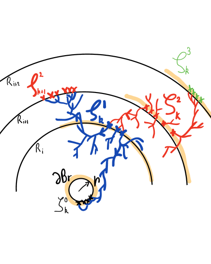
Figure 1: Waves

By monotone convergence, we deduce that for any $\lambda$ and $\lambda^{\prime}$,

$$\varphi_{r,i+1}(\lambda)\leq\lim_{n\to\infty}\sup_{x\in\partial B_{R_{i+1}}}\mathbb{E}_{x}\Big{[}\exp\big{(}\frac{\lambda\sum_{k=0}^{n}|\zeta_{k}^{0}|}{r^{2}}+\frac{\lambda\sum_{k=0}^{n}|\zeta^{3}_{k}|}{R_{i+2}^{2}}\big{)}\Big{]}.$$ (7.7)

For $k\geq 0$, we let $\mathcal{G}_{k}$ be the sigma-field generated by the tree $\mathcal{T}$ cut at vertices in $\zeta_{k}^{1}\cup\zeta_{k}^{3}$, together with the positions of the BRW at the vertices on this subtree. We also let $\mathcal{H}_{k}$ be the sigma-field generated by the tree cut at vertices in $\zeta_{k}^{2}$, together with the positions of the BRW on the corresponding subtree.

Now fix $\lambda\leq\lambda_{1}$. The induction hypothesis implies that almost surely, one has

$$\mathbb{E}_{x}\Big{[}\exp\big{(}\frac{\lambda|\zeta_{n}^{0}|}{r^{2}}\big{)}\ \big{|}\ \mathcal{G}_{n}\Big{]}\leq\exp\big{(}\frac{\lambda|\zeta_{n}^{1}|}{R_{i}^{2}}\big{)}.$$

Then Lemma 7.3 ensures, that for $0\leq\lambda\leq\lambda_{0}$, and $r\geq r_{0}$, almost surely (recall (7.6)),

$$\mathbb{E}_{x}\Big{[}\exp\big{(}\frac{\lambda|\zeta_{n}^{1}|}{R_{i}^{2}}+\frac{\lambda|\zeta^{3}_{n}|}{R_{i+2}^{2}}\big{)}\ \big{|}\ \mathcal{H}_{n}\Big{]}\leq\exp\big{(}\frac{\lambda|\zeta_{n}^{2}|}{R_{i+1}^{2}}\big{)}.$$

Note that one can always assume $\lambda_{1}$ to be smaller than $\lambda_{0}$, so that the condition $\lambda\leq\lambda_{0}$ is well satisfied under our standing hypothesis on $\lambda$. Applying again the induction hypothesis, we get that almost surely,

$$\mathbb{E}_{x}\Big{[}\exp\big{(}\frac{\lambda|\zeta_{n-1}^{0}|}{r^{2}}+\frac{\lambda|\zeta^{2}_{n}|}{R_{i+1}^{2}}\big{)}\ \big{|}\ \mathcal{G}_{n-1}\Big{]}\leq\exp\big{(}\frac{\lambda|\zeta_{n-1}^{1}|}{R_{i}^{2}}\big{)}.$$

Then an elementary induction shows that for all $n\geq 1$,

$$\mathbb{E}_{x}\Big{[}\exp\big{(}\frac{\lambda\sum_{k=0}^{n}|\zeta_{k}^{0}|}{r^{2}}+\frac{\lambda^{\prime}\sum_{k=0}^{n}|\zeta^{3}_{k}|}{R_{i+2}^{2}}\big{)}\Big{]}\leq\exp\big{(}\frac{\lambda}{R_{i+1}^{2}}\big{)},$$

proving (7.5) for $i+1$, with the same constant $\lambda_{1}$. This concludes the proof of Proposition 7.1. ∎

8 Proof of Theorem 1.6

The proof is similar to the proof of Theorem 1.5, but one has to be slightly more careful. The main difference comes from the following modified version of Proposition 7.1.

Proposition 8.1.

Assume $d=4$. There exist positive constants $c$ and $\lambda_{0}$, such that for any $r\geq 1$, $R\geq r$, and $0\leq\lambda\leq\lambda_{0}$,

$$\sup_{R\leq\|z\|\leq 2R}\mathbb{E}_{z}\Big{[}\exp\big{(}\lambda\frac{|\eta_{r,2R}|}{r^{2}\log(R/r)}\big{)}\Big{]}\leq\exp\big{(}\frac{c\lambda}{R^{2}\log(R/r)}\big{)}.$$

Once this proposition is established, the end of the proof of Theorem 1.6 is almost the same as in dimension five and higher. Indeed, let us postpone the proof of Proposition 8.1 for a moment, and conclude the proof of Theorem 1.6 first.

Proof of Theorem 1.6.

Let $r\geq 1$, and $R\geq 2r$ be given, and let also $x$ be such that $2r\leq\|x\|\leq R$. Let $i_{0}$ be the smallest integer, such that $\|x\|\leq r2^{i_{0}}$, and let $I$ be the smallest integer such that $R\leq r2^{i_{0}+I}$. Recall the definition (7.1) of $R_{i}$ and $Z_{r,i}$, and notice that

$$|\eta_{r,R}|\leq\sum_{i=0}^{I}Z_{r,i}.$$

Moreover, as in the proof of Theorem 1.5, on one hand Proposition 8.1 shows that (with the same constant $c$ as in its statement),

$$\mathbb{E}_{x}\Big{[}\exp\big{(}\frac{\lambda}{r^{2}\log(R/r)}\sum_{i=0}^{I}Z_{r,i}\big{)}\Big{]}\leq\exp\big{(}\frac{c\lambda}{\|x\|^{2}\log(R/r)}\big{)}\cdot\mathbb{E}_{x}\Big{[}\exp\big{(}\frac{2c\lambda}{\log(R/r)}\cdot\sum_{i=0}^{I}\frac{|\eta_{R_{i}}|}{R_{i}^{2}}\big{)}\Big{]},$$

and on the other hand, using (1.9), we get by induction

$$\mathbb{E}_{x}\Big{[}\exp\big{(}\frac{2c\lambda}{\log(R/r)}\cdot\sum_{i=0}^{I}\frac{|\eta_{R_{i}}|}{R_{i}^{2}}\big{)}\Big{]}\leq\exp\big{(}\frac{8c\lambda}{\|x\|^{2}\log(R/r)}\big{)},$$

which concludes the proof of (1.14). The proof of (1.15) follows exactly as for the corresponding statement in Theorem 1.3, namely (1.8), using Lemma 3.5. Finally concerning the proof of (1.16), one can argue as follows. First using the first point of Lemma 3.8, one has for some constant $\varepsilon>0$,

$$\mathbb{E}_{x}\Big{[}\exp\big{(}\frac{\lambda|\eta_{r,R}|}{r^{2}\log(R/r)}\big{)}\Big{]}\leq \ 1+\frac{(1-\varepsilon)\lambda}{r^{2}\log(R/r)}+\frac{\lambda^{2}}{r^{4}\log(R/r)^{2}}\mathbb{E}_{x}\Big{[}|\eta_{r,R}|^{2}\exp\big{(}\frac{2\lambda|\eta_{r,R}|}{r^{2}\log(R/r)}\big{)}\Big{]}.$$

Then, using Proposition 3.11 and Hölder’s inequality at the third line, and (1.15) and the second point of Lemma 3.8 at the last one, we get

$$\mathbb{E}_{x}\Big{[}\exp\big{(}\frac{\lambda|\eta_{r,R}|}{r^{2}\log(R/r)}\big{)}\Big{]}$$

$$\leq 1+\frac{(1-\varepsilon)\lambda}{r^{2}\log(R/r)}+\frac{\lambda^{2}}{r^{4}\log(R/r)^{2}}\mathbb{E}_{x}\Big{[}|\eta_{r,R}|^{2}\exp\big{(}\frac{2\lambda|\eta_{r,R}|}{r^{2}\log(R/r)}\big{)}\ \Big{|}\ \eta_{r,R}\neq\varnothing\Big{]}\cdot\mathbb{P}_{x}(|\eta_{r,R}|>0)$$

$$\leq 1+\frac{(1-\varepsilon)\lambda}{r^{2}\log(R/r)}+\frac{c\lambda^{2}}{r^{4+2/3}\log(R/r)^{2}}\mathbb{E}_{x}\big{[}|\eta_{r}|^{3}\big{]}^{2/3}\cdot\mathbb{E}_{x}\Big{[}\exp\big{(}\frac{3\lambda|\eta_{r,R}|}{r^{2}\log(R/r)}\big{)}\ \Big{|}\ \eta_{r,R}\neq\varnothing\Big{]}^{1/3}$$

$$\leq 1+\frac{(1-\varepsilon)\lambda}{r^{2}\log(R/r)}+\frac{c\lambda^{2}}{r^{2}\log(R/r)^{2}}\leq\exp\big{(}\frac{(1-\varepsilon^{\prime})\lambda}{r^{2}\log(R/r)}\big{)},$$

for some constant $\varepsilon^{\prime}\in(0,1)$, proving well (1.16). This concludes the proof of Theorem 1.6. ∎

It remains now to prove Proposition 8.1, which requires some more care than for the proof of Proposition 7.1. In particular one needs first to strengthen Lemma 7.3.

Lemma 8.2.

Assume $d=4$. There exists positive constants $c$ and $\lambda_{0}$, such that for any $0\leq\lambda,\lambda^{\prime}\leq\lambda_{0}$, and any $r\geq 1$,

$$\sup_{x\in\partial B_{2r}}\mathbb{E}_{x}\Big{[}\exp\big{(}\lambda\frac{|\eta_{r,4r}|}{r^{2}}+\lambda^{\prime}\frac{|\eta_{4r,r}|}{4r^{2}}\big{)}\Big{]}\leq\exp\Big{(}\frac{\lambda(1+\frac{c}{r}+c\lambda)+\lambda^{\prime}(1+\frac{c}{r}+c\lambda^{\prime})}{5r^{2}}\Big{)}.$$

Proof.

The proof is similar to the proof of Lemma 7.3. First we write for any $x\in\partial B_{2r}$,

$$\mathbb{E}_{x}\Big{[}\exp\big{(}\frac{\lambda|\eta_{r,4r}|}{r^{2}}\big{)}\Big{]}\leq 1+\frac{\lambda\mathbb{E}_{x}\big{[}|\eta_{r,4r}|\big{]}}{r^{2}}+\frac{\lambda^{2}}{r^{4}}\mathbb{E}_{x}\Big{[}|\eta_{r,4r}|^{2}\exp\big{(}\frac{\lambda|\eta_{r,4r}|}{r^{2}}\big{)}\Big{]},$$

and

$$\mathbb{E}_{x}\big{[}|\eta_{r,4r}|\big{]}=\mathbf{P}_{x}(H_{r}<H_{4r})\leq\frac{G(x)-G(4r)}{G(r)-G(4r)},$$

with $G(s)=\inf_{z\in\partial B_{s}}G(z)$, for $s\geq 1$. Using (2.5), we deduce that in dimension four, for some constant $c>0$,

$$\sup_{x\in\partial B_{2r}}\mathbb{E}_{x}\big{[}|\eta_{r,4r}|\big{]}\leq\frac{1}{5}(1+c/r).$$

We conclude as in the proof of Lemma 7.3 that for $\lambda$ small enough,

$$\sup_{x\in\partial B_{2r}}\mathbb{E}_{x}\Big{[}\exp\big{(}\frac{\lambda|\eta_{r,4r}|}{r^{2}}\big{)}\Big{]}\leq\exp\big{(}\frac{\lambda(1+\frac{c}{r}+c\lambda)}{5r^{2}}\big{)}.$$

The same argument leads to

$$\sup_{x\in\partial B_{2r}}\mathbb{E}_{x}\Big{[}\exp\big{(}\frac{\lambda^{\prime}|\eta_{4r,r}|}{4r^{2}}\big{)}\Big{]}\leq\exp\big{(}\frac{\lambda^{\prime}(1+\frac{c}{r}+c\lambda^{\prime})}{5r^{2}}\big{)},$$

and the lemma follows using Cauchy-Schwarz inequality. ∎

Proof of Proposition 8.1.

As for the proof of Proposition 7.1 it suffices to prove the result for $r$ large enough, and for $R$ of the form $R_{i}=r2^{i}$, with $i\geq 1$. Now we consider the function

$$\psi_{r,i}(\lambda,\lambda^{\prime}):=\sup_{x\in\partial B_{R_{i}}}\mathbb{E}_{x}\Big{[}\exp\big{(}\frac{\lambda|\eta_{r,R_{i+1}}|}{ir^{2}}+\frac{\lambda^{\prime}|\eta_{R_{i+1},r}|}{iR_{i}^{2}}\big{)}\Big{]},$$

and claim that there exist positive constants $r_{0}$, $\kappa$ and $\lambda_{1}$, such that for all $r\geq r_{0}$, all $i\geq 1$, and all $0\leq\lambda\leq\lambda^{\prime}\leq\lambda_{1}$,

$$\psi_{r,i}(\lambda,\lambda^{\prime})\leq\exp\Big{(}\frac{\alpha_{i}(\lambda+\lambda^{\prime})\cdot\lambda+\beta_{i}(\lambda+\lambda^{\prime})\cdot\lambda^{\prime}}{iR_{i}^{2}}\Big{)},$$ (8.1)

writing for $t\geq 0$,

$$\alpha_{i}(t):=\prod_{j=1}^{i}(1+\frac{\kappa}{R_{j}}+\frac{\kappa t}{i}),\quad\text{and}\quad\beta_{i}(t)=1+\frac{\kappa}{R_{i}}+\frac{\kappa t}{i}.$$

As mentioned above, we note that this would imply the proposition.

We prove (8.1) by induction. The result for $i=1$ is given by Lemma 8.2. Assume now that it holds for some $i\geq 1$, and let us prove it for $i+1$. Define $\{\zeta_{k}^{j}\}_{k\geq 0}$, for $j\in\{0,1,2,3\}$, as well as $\{\mathcal{G}_{k}\}_{k\geq 0}$ and $\{\mathcal{H}_{k}\}_{k\geq 0}$, as in the proof of Proposition 7.1. Recall that by monotone convergence, one has

$$\psi_{r,i+1}(\lambda,\lambda^{\prime})\leq\lim_{n\to\infty}\sup_{x\in\partial B_{R_{i+1}}}\mathbb{E}_{x}\Big{[}\exp\big{(}\frac{\lambda\sum_{k=0}^{n}|\zeta_{k}^{0}|}{(i+1)r^{2}}+\frac{\lambda^{\prime}\sum_{k=0}^{n}|\zeta^{3}_{k}|}{(i+1)R_{i+1}^{2}}\big{)}\Big{]}.$$ (8.2)

Fix $\lambda,\lambda^{\prime}$ such that $0\leq\lambda\leq\lambda^{\prime}\leq\lambda_{1}$, where $\lambda_{1}$ is given by the induction hypothesis. The latter implies that almost surely,

$$\mathbb{E}_{x}\Big{[}\exp\big{(}\frac{\lambda|\zeta_{n}^{0}|}{(i+1)r^{2}}\big{)}\ \big{|}\ \mathcal{G}_{n}\Big{]}\leq\exp\big{(}\frac{\alpha\lambda|\zeta_{n}^{1}|}{(i+1)R_{i}^{2}}\big{)},\qquad\text{with }\alpha:=\alpha_{i}(\frac{i(\lambda+\lambda^{\prime})}{i+1}).$$

Define now, with $c$ the constant appearing in Lemma 8.2,

$$\rho:=1+\frac{c}{R_{i+1}}+\frac{2c(\lambda+\lambda^{\prime})}{i+1},\quad\text{and}\quad\nu:=1+\frac{\kappa}{R_{i}}+\frac{\kappa(\lambda+\lambda^{\prime})}{i+1}.$$

Note that we may assume that $\lambda_{1}$ is small enough, and $r_{0}$ large enough, to ensure that $\lambda_{1}\alpha$ is smaller than the constant $\lambda_{0}$ from Lemma 8.2. Likewise we may always assume that $\alpha\leq 2$ (whence the constant $2$ appearing in the definition of $\rho$). Then the latter yields almost surely

$$\mathbb{E}_{x}\Big{[}\exp\big{(}\frac{\alpha\lambda|\zeta_{n}^{1}|}{(i+1)R_{i}^{2}}+\frac{\lambda^{\prime}|\zeta^{3}_{n}|}{(i+1)R_{i+1}^{2}}\big{)}\ \big{|}\ \mathcal{H}_{n}\Big{]}\leq\exp\big{(}\frac{\rho(\alpha\lambda+\lambda^{\prime})|\zeta_{n}^{2}|}{5(i+1)R_{i}^{2}}\big{)}.$$

Observe next that we may further assume (since we take $\lambda\leq\lambda^{\prime}$ by assumption) that

$$\frac{\rho}{5}(\alpha\lambda+\lambda^{\prime})\leq\lambda^{\prime}.$$

Thus applying again the induction hypothesis, we get that almost surely,

$$\mathbb{E}_{x}\Big{[}\exp\big{(}\frac{\lambda|\zeta_{n-1}^{0}|}{(i+1)r^{2}}+\frac{\rho(\alpha\lambda+\lambda^{\prime})|\zeta_{n}^{2}|}{5(i+1)R_{i}^{2}}\big{)}\ \big{|}\ \mathcal{G}_{n-1}\Big{]}\leq\exp\Big{(}\big{\{}\alpha\lambda(1+\frac{\rho\nu}{5})+\frac{\rho\nu\lambda^{\prime}}{5}\big{\}}\cdot\frac{|\zeta_{n-1}^{1}|}{(i+1)R_{i}^{2}}\Big{)}.$$

Another application of Lemma 8.2 gives

$$\mathbb{E}_{x}\Big{[}\exp\Big{(}\big{\{}\alpha\lambda(1+\frac{\rho\nu}{5})+\frac{\rho\nu\lambda^{\prime}}{5}\big{\}}\cdot\frac{|\zeta_{n-1}^{1}|}{(i+1)R_{i}^{2}}+\frac{\lambda^{\prime}|\zeta_{n-1}^{3}|}{(i+1)R_{i+1}^{2}}\Big{)}\ \Big{|}\ \mathcal{G}_{n-1}\Big{]}$$

$$\leq\exp\Big{(}\big{(}\alpha\lambda+\lambda^{\prime}\big{)}\cdot(1+\frac{\rho\nu}{5})\cdot\frac{\rho|\zeta_{n}^{2}|}{5(i+1)R_{i}^{2}}\Big{)}.$$

Then an elementary induction shows that for all $n\geq 1$,

$$\mathbb{E}_{x}\Big{[}\exp\big{(}\frac{\lambda\sum_{k=0}^{n}|\zeta_{k}^{0}|}{(i+1)r^{2}}+\frac{\lambda^{\prime}\sum_{k=0}^{n}|\zeta^{3}_{k}|}{(i+1)R_{i+1}^{2}}\big{)}\Big{]}\leq\exp\Big{(}\frac{4\rho}{5}\cdot\frac{\alpha\lambda+\lambda^{\prime}}{(i+1)R_{i+1}^{2}}\cdot\sum_{k=0}^{n}(\frac{\rho\nu}{5})^{k}\Big{)}.$$

To conclude, note that

$$\rho\sum_{k=0}^{\infty}(\frac{\rho\nu}{5})^{k}=\frac{5\rho}{5-\rho\nu}\leq\frac{5}{4}\cdot\big{(}1+\frac{\kappa}{R_{i+1}^{2}}+\frac{\kappa(\lambda+\lambda^{\prime})}{i+1}\big{)}=\frac{5}{4}\beta_{i+1}(\lambda+\lambda^{\prime}),$$

at least provided we first choose $r_{0}$ and $\kappa$ large enough (compared to $c$), and then $\lambda_{1}$ small enough. Finally notice that $\alpha\beta_{i+1}(\lambda+\lambda^{\prime})=\alpha_{i+1}(\lambda+\lambda^{\prime})$, thereby finishing the proof of the induction step for (8.1). This concludes the proof of Proposition 8.1. ∎

9 Proof of Theorem 1.1: upper bounds in $d\geq 4$

The proof in dimension four is slightly different from the higher dimensional case, but first one needs to strengthen the result of Proposition 1.4 as follows. Recall that we denote by $\mathcal{T}(B_{r})$ the time spent in the ball $B_{r}$ by a BRW, for which we freeze the particles reaching the boundary of the ball, see (1.5).

Proposition 9.1.

Assume $d\geq 1$. There exist positive constants $c$ and $C$, such that for all $r\geq 1$, and all $t\geq r^{4}$,

$$\sup_{x\in B_{r}}\mathbb{P}_{x}(|\mathcal{T}(B_{r})|>t)\leq\frac{C}{r^{2}}\exp(-ct/r^{4}).$$

Proof.

Given $u\in\mathcal{T}$, and $\Lambda\subset\mathbb{Z}^{d}$, we call $\mathcal{T}^{u}(\Lambda)$ the random variable with the same law as $\mathcal{T}(\Lambda)$ shifted in the subtree emanating from $u$. Recall also that $\mathcal{T}_{n}=\{u\in\mathcal{T}:|u|\leq n\}$, and assume without loss of generality that $r^{2}$ is an integer. One has

$$\mathbb{P}_{x}(|\mathcal{T}(B_{r})|>t)\leq\mathbb{P}_{x}\Big{(}\sum_{|u|=r^{2}}|\mathcal{T}^{u}(B_{r})|\geq t/2\Big{)}+\mathbb{P}\big{(}|\mathcal{T}_{r^{2}}|>t/2\big{)}.$$ (9.1)

For the first term on the right-hand side we use first Proposition 1.4 and Chebyshev’s exponential inequality, which give for any $\lambda$ small enough,

$$\mathbb{P}_{x}\Big{(}\sum_{|u|=r^{2}}|\mathcal{T}^{u}(B_{r})|\geq t/2\Big{)}\leq e^{-\frac{\lambda t}{2r^{4}}}\cdot\mathbb{E}\Big{[}\exp\big{(}c\lambda\frac{Z_{r^{2}}}{r^{2}}\big{)}\ \Big{|}\ Z_{r^{2}}\neq 0\Big{]}\cdot\mathbb{P}(Z_{r^{2}}\neq 0).$$

Then Lemma 3.1 and (2.2) yield for some constant $C>0$,

$$\mathbb{P}_{x}\Big{(}\sum_{|u|=r^{2}}|\mathcal{T}^{u}(B_{r})|\geq t/2\Big{)}\leq\frac{C}{r^{2}}\exp(-\frac{\lambda t}{2r^{4}}).$$

Concerning now the second term on the right-hand side of (9.1), we use a similar idea. Let $I$ be the smallest integer, such that $r^{2}\leq 2^{I}$. Using this time both Lemmas  3.1 and 3.2 shows that for some $\lambda$ small enough, and positive constants $c$, and $C$,

$$\mathbb{P}\big{(}|\mathcal{T}_{r^{2}}|>t/2\big{)} \leq\sum_{i=0}^{I-1}\mathbb{P}\big{(}\sum_{k=2^{i}}^{2^{i+1}}Z_{k}>2^{i-I-1}t\big{)}$$

$$\leq\sum_{i=0}^{I-1}\exp\big{(}-\frac{\lambda 2^{i-I-1}t}{2^{2i}}\big{)}\cdot\mathbb{E}\Big{[}\exp\big{(}\frac{c\lambda Z_{2^{i}}}{2^{i}}\big{)}\ \Big{|}\ Z_{2^{i}}\neq 0\Big{]}\cdot\mathbb{P}(Z_{2^{i}}\neq 0)$$

$$\leq\frac{C}{r^{2}}\sum_{i=0}^{I-1}2^{I-i}\exp\big{(}-\frac{\lambda 2^{I-i}t}{8r^{4}}\big{)}\leq\frac{C}{r^{2}}\exp(-\frac{\lambda t}{8r^{4}}),$$

using $t\geq r^{4}$, for the last inequality. This concludes the proof of the proposition. ∎

We can now finish the proof of the upper bounds in Theorem 1.1 in dimensions four and higher.

Assume first that $d\geq 5$. Define two sequences $\{\zeta_{k}^{j}\}_{k\geq 0}$, for $j=1,2$, by $\zeta_{0}^{1}=\{\varnothing\}$ is the root of the tree, and for $k\geq 0$,

$$\zeta_{k}^{2}:=\bigcup_{u\in\zeta_{k}^{1}}\eta^{u}_{2r},\quad\text{and}\quad\zeta_{k+1}^{1}:=\bigcup_{u\in\zeta_{k}^{2}}\eta^{u}_{r}.$$

Let also for $k\geq 0$,

$$L_{k}(B_{r}):=\sum_{u\in\zeta_{k}^{1}}|\mathcal{T}^{u}(B_{2r})|,$$

with the notation from the proof of the previous proposition. Then by definition, one has

$$\ell_{\mathcal{T}}(B_{r})\leq\sum_{k\geq 0}L_{k}(B_{r}).$$

Therefore by Proposition 3.10, for any $\lambda>0$,

$$\mathbb{P}\big{(}\ell_{\mathcal{T}}(B_{r})>t\big{)}\leq\mathbb{P}\big{(}|\mathcal{T}(B_{2r})|>t/2\big{)}+\frac{C}{r^{2}}\exp(-\frac{\lambda t}{2r^{4}})\cdot\mathbb{E}\Big{[}\exp\big{(}\frac{\lambda}{r^{4}}\sum_{k\geq 1}L_{k}(B_{r})\big{)}\ \Big{|}\ |\eta_{r}|>0\Big{]}.$$

The first term on the right-hand side is ruled out by Proposition 9.1. Hence only the last expectation is at stake, and it just amounts to show that it is bounded. By monotone convergence one has

$$\mathbb{E}\Big{[}\exp\big{(}\frac{\lambda}{r^{4}}\sum_{k\geq 1}L_{k}(B_{r})\big{)}\ \Big{|}\ |\eta_{r}|>0\Big{]}=\lim_{n\to\infty}\mathbb{E}\Big{[}\exp\big{(}\frac{\lambda}{r^{4}}\sum_{k=1}^{n}L_{k}(B_{r})\big{)}\ \Big{|}\ |\eta_{r}|>0\Big{]}.$$

Note also that if $\mathcal{G}_{n}$ denotes the sigma-field generated by the BGW tree cut at vertices in $\zeta_{n}^{1}$, together with the positions of the BRW on this subtree, then by Proposition 1.4, almost surely for all $\lambda$ small enough,

$$\mathbb{E}\Big{[}\exp\big{(}\frac{\lambda L_{n}(B_{r})}{r^{4}}\big{)}\ \Big{|}\ \mathcal{G}_{n}\Big{]}\leq\exp\big{(}\frac{c\lambda|\zeta_{n}^{1}|}{r^{2}}\big{)},$$

for some constant $c>0$. It follows that for any $n\geq 0$,

$$\mathbb{E}\Big{[}\exp\Big{(}\frac{\lambda}{r^{4}}\sum_{k=1}^{n}L_{k}(B_{r})-\frac{c\lambda}{r^{2}}\sum_{k=1}^{n}|\zeta_{k}^{1}|\Big{)}\ \Big{|}\ |\eta_{r}|>0\Big{]}\leq 1.$$

Hence by Cauchy-Schwarz, it just amounts to show that for $\lambda$ small enough, the sequence $\{u_{n}(\lambda)\}_{n\geq 1}$ defined by

$$u_{n}(\lambda):=\mathbb{E}\Big{[}\exp\Big{(}\frac{c\lambda}{r^{2}}\sum_{k=1}^{n}|\zeta_{k}^{1}|\Big{)}\ \Big{|}\ |\eta_{r}|>0\Big{]},$$

is bounded. By combining Theorems 1.9 and 1.12, we get that for $\lambda$ small enough, and some $\varepsilon>0$, one has for any $k\geq 2$, almost surely

$$\mathbb{E}\Big{[}\exp\Big{(}\frac{\lambda}{r^{2}}|\zeta_{k}^{1}|\Big{)}\ \Big{|}\ \mathcal{G}_{k-1}\Big{]}\leq\exp\big{(}\frac{(1-\varepsilon)\lambda}{r^{2}}|\zeta_{k-1}^{1}|\big{)},$$

and using also (1.8), we get for some constant $c^{\prime}>0$,

$$\mathbb{E}\Big{[}\exp\Big{(}\frac{\lambda}{r^{2}}|\zeta_{1}^{1}|\Big{)}\ \Big{|}\ |\eta_{r}|>0\Big{]}\leq\exp(c^{\prime}\lambda).$$

We deduce that for any $n\geq 1$, and $\lambda$ small, that $\{u_{n}(\lambda)\}_{n\geq 1}$ is bounded through

$$u_{n}(\lambda)\leq\exp\big{(}c^{\prime}\lambda\sum_{k=0}^{n}(1-\varepsilon)^{k})\leq\exp(c^{\prime}\lambda/\varepsilon),$$

This concludes the proof of the upper bound in Theorem 1.1, in case $d\geq 5$.

In the case when $d=4$, the proof follows similar pattern, but we need to consider a truncated deposition process on $B_{r}$. Instead of $\{\zeta_{k}^{j}\}_{k\geq 0}$, set $\widetilde{\zeta}_{0}^{1}=\{\varnothing\}$, and with $R=r2^{I}$, and $I:=\sqrt{t/r^{4}}$, we define for $k\geq 0$,

$$\widetilde{\zeta}_{k}^{2}:=\bigcup_{u\in\widetilde{\zeta}_{k}^{1}}\eta^{u}_{2r},\quad\text{and}\quad\widetilde{\zeta}_{k+1}^{1}:=\bigcup_{u\in\widetilde{\zeta}_{k}^{2}}\eta^{u}_{r,R}.$$

Then we define similarly for $k\geq 0$,

$$L_{k}(B_{r}):=\sum_{u\in\widetilde{\zeta}_{k}^{1}}|\mathcal{T}^{u}(B_{2r})|,$$

and Chebychev’s inequality reads

$$\begin{split}\mathbb{P}\big{(}\ell_{\mathcal{T}}(B_{r})>t\big{)}\leq&\mathbb{P}\big{(}|\mathcal{T}(B_{2r})|>\frac{t}{2}\big{)}+\mathbb{P}(|\eta_{R}|>0)\\ &\qquad+\frac{C}{r^{2}}e^{-\frac{\lambda t}{2Ir^{4}}}\cdot\mathbb{E}\Big{[}\exp\big{(}\frac{\lambda}{Ir^{4}}\sum_{k\geq 1}L_{k}(B_{r})\big{)}\ \Big{|}\ |\eta_{r}|>0\Big{]}.\end{split}$$ (9.2)

The second term is $\mathcal{O}(1/R^{2})$ by Proposition 3.10, and the other terms are ruled out exactly as in higher dimension, using the estimates from Theorem 1.6, instead as from Theorem 1.5. $\square$

10 Proof of Theorem 1.1: lower bounds in $d\geq 4$

We start with the case of dimension five and higher, and consider the subtle case of dimension four separately.

10.1 Dimension five and higher

Assume $d\geq 5$, and recall that we may also assume here that $t\geq r^{4}$. The strategy we will use is to ask the BRW to reach $\partial B_{r}$ (at a cost of order $1/r^{2}$), and then make order $t/r^{4}$ excursions (or waves) between $\partial B_{r}$ and $\partial B_{r/2}$, at a cost of order $\exp(-\Theta(t/r^{4}))$.

More precisely, the proof relies on the following lemma, which holds in fact in any dimension (recall (1.6)).

Lemma 10.1.

Assume $d\geq 1$. There exists a constant $c>0$, such that for any $r\geq 1$,

$$\inf_{x\in B_{r/2}\cup\partial B_{2r}}\,\mathbb{P}_{x}(|\eta_{r}|\geq cr^{2})\geq c/r^{2}.$$

Proof.

Let

$$\overline{\eta}_{r}:=\{u\in\eta_{r}:r^{2}\leq|u|\leq 2r^{2}\}.$$

Note that uniformly over $x\in B_{r/2}\cup\partial B_{2r}$,

$$\mathbb{E}_{x}[|\overline{\eta}_{r}|]=\sum_{n=r^{2}}^{2r^{2}}\mathbb{E}[Z_{n}]\cdot\mathbf{P}_{x}(H_{r}=n)=\mathbf{P}_{x}(r^{2}\leq H_{r}\leq 2r^{2})\gtrsim 1,$$

and using a similar computation as in Subsection 3.3,

$$\mathbb{E}_{x}\big{[}|\overline{\eta}_{r}|^{2}\big{]}=\mathbb{E}_{x}[|\overline{\eta}_{r}|]+\sigma^{2}\,\sum_{k=0}^{r^{2}-1}\mathbf{E}_{x}\big{[}{\text{\Large$\mathfrak{1}$}}\{H_{r}>k\}\cdot\mathbf{P}_{S_{k}}\big{(}r^{2}-k\leq H_{r}\leq 2r^{2}-k\big{)}^{2}\big{]}\leq 1+\sigma^{2}r^{2}.$$

Now by (2.2),

$$\mathbb{P}_{x}(|\overline{\eta}_{r}|>0)\leq\mathbb{P}(Z_{r^{2}}\neq 0)\lesssim 1/r^{2}.$$

Therefore,

$$\mathbb{E}_{x}\big{[}|\overline{\eta}_{r}|\mid|\overline{\eta}_{r}|>0\big{]}\gtrsim r^{2},$$

and Paley-Zygmund’s inequality (2.8) gives, for some constant $c>0$,

$$\mathbb{P}_{x}\left(|\overline{\eta}_{r}|>cr^{2}\right)\gtrsim 1/r^{2}.$$

Since $\overline{\eta}_{r}\subset\eta_{r}$, this proves the lemma. ∎

Consequently, if we start with order $r^{2}$ particles on $\partial B_{r}$, then with probability of order $1$, there will be order $r^{2}$ particles reaching $\partial B_{r/2}$. Repeating this argument we see that with probability at least $\Theta(1/r^{2})\cdot\exp(-\Theta(t/r^{4}))$, the BRW will make at least $\Theta(t/r^{4})$ waves between $\partial B_{r}$ and $\partial B_{r/2}$, with an implicit constant as large as wanted. The expected time spent on $B_{r}$ by each of these waves is of order $r^{4}$, simply because for any starting point on $\partial B_{r/2}$, the expected time spent on $B_{r}$ by the BRW killed on $\partial B_{r}$ is of order $r^{2}$. Since all the waves are independent of each other (at least conditionally on the positions of the frozen particles), we shall deduce that the total time spent on $B_{r}$ will exceed $t$.

On a formal level now, we define $\{\zeta_{k}^{1}\}_{k\geq 0}$, $\{\zeta_{k}^{1,1}\}_{k\geq 0}$ and $\{\zeta_{k}^{2}\}_{k\geq 0}$ inductively by $\zeta_{0}^{1,1}=\zeta_{0}^{1}=\{\varnothing\}$ (the root of the tree), and then for $k\geq 0$,

$$\zeta_{k}^{2}=\bigcup_{u\in\zeta_{k}^{1,1}}\eta^{u}_{r},\qquad\zeta_{k+1}^{1}=\bigcup_{u\in\zeta_{k}^{2}}\eta^{u}_{r/2},$$

and for $\zeta_{k+1}^{1,1}$ we take any subset (chosen arbitrarily, for instance uniformly at random) of $\zeta_{k+1}^{1}$ with $\lceil|\zeta_{k+1}^{1}|/2\rceil$ points. We also let $\zeta_{k}^{1,2}:=\zeta_{k}^{1}\setminus\zeta_{k}^{1,1}$, for $k\geq 0$. Next, set $N:=\lceil Ct/r^{4}\rceil$, with $C>0$ some large constant to be fixed later, and define further for $k\geq 1$,

$$L_{k}(B_{r}):=\sum_{u\in\zeta_{k}^{1,2}}|\mathcal{T}^{u}(B_{r})|,$$

with the notation from the proof of Proposition 9.1. The reason why we partition the sets $\zeta_{k}^{1}$ into two parts, is that we want to keep, for each $k\geq 1$, some independence between $\zeta_{k}^{2}$ and $L_{k}(B_{r})$, conditionally on $\zeta_{k}^{1}$. Now, note that

$$\ell_{\mathcal{T}}(B_{r})\geq\sum_{k=1}^{N}L_{k}(B_{r}).$$ (10.1)

For $k\geq 1$, define $\mathcal{G}_{k}$ as the sigma-field generated by tree cut at vertices in $\zeta_{k}^{1}$, together with the choice of $\zeta_{k}^{1,1}$ and the positions of the BRW on the vertices of this subtree. Let also $E_{k}:=\{|\zeta_{k}^{1,1}|\geq cr^{2}\}$, with $c$ chosen such that

$$\rho:=\min\Big{(}\mathbb{P}(E_{1}),\inf_{k\geq 2}\mathbb{P}(E_{k}\mid E_{k-1})\Big{)}>0.$$ (10.2)

Note that the existence of $c$ is guaranteed by Lemma 10.1. Observe also that $E_{k}\in\mathcal{G}_{k}$, for any $k\geq 1$. Remember next that for some constant $c^{\prime}>0$, one has for all $r\geq 1$,

$$\inf_{x\in\partial B_{r/2}}\mathbb{E}_{x}\big{[}|\mathcal{T}(B_{r})|\big{]}=\inf_{x\in\partial B_{r/2}}\mathbf{E}_{x}[H_{r}]\geq c^{\prime}r^{2}.$$

As a consequence, for any $k\geq 1$, almost surely,

$$\mathbb{E}\big{[}L_{k}(B_{r})\mid\mathcal{G}_{k}]\geq c^{\prime}r^{2}|\zeta_{k}^{1,2}|.$$

On the other hand,

$$\sup_{x\in B_{r}}\mathbb{E}_{x}\big{[}|\mathcal{T}(B_{r})|\big{]}=\sup_{x\in B_{r}}\mathbf{E}_{x}[H_{r}]=\mathcal{O}(r^{2}),$$

which entails that for some constant $K>0$, for any $x\in B_{r}$,

$$\mathbb{E}_{x}\big{[}|\mathcal{T}(B_{r})|^{2}\big{]}\leq\mathbb{E}_{x}\big{[}|\mathcal{T}(B_{r})|\big{]}+\sum_{k=0}^{\infty}\mathbb{E}_{x}\Big{[}\sum_{\begin{subarray}{c}u\in\mathcal{T}(B_{r})\\ |u|=k\end{subarray}}\xi_{u}(\xi_{u}-1)\Big{(}\sup_{z\in B_{r}}\mathbb{E}_{z}\big{[}|\mathcal{T}(B_{r})|\big{]}\Big{)}^{2}\Big{]}\leq Kr^{6}.$$

As a consequence, one has for any $k\geq 0$,

$$\mathbb{E}\big{[}L_{k}(B_{r})^{2}\mid\mathcal{G}_{k}\big{]}\leq Kr^{6}|\zeta_{k}^{1,2}|.$$

Using then Paley-Zygmund’s inequality (2.7) we get

$$\mathbb{P}(F_{k}\mid\mathcal{G}_{k}){\text{\Large$\mathfrak{1}$}}_{E_{k}}\geq\frac{cc^{\prime 2}}{4K}{\text{\Large$\mathfrak{1}$}}_{E_{k}},\quad\text{with}\quad F_{k}:=\Big{\{}L_{k}(B_{r})\geq\frac{cc^{\prime}r^{4}}{2}\Big{\}}.$$ (10.3)

Note now that on the event

$$\widetilde{E}_{N}:=\bigcap_{k=1}^{N}E_{k}\cap F_{k},$$

by (10.1) one has $\ell_{\mathcal{T}}(B_{r})\geq Ncc^{\prime}r^{4}/2$, which is larger than $t$, provided the constant $C$ in the definition of $N$ is chosen large enough. Moreover, for each $k\geq 0$, conditionally on $\mathcal{G}_{k}$, $E_{k+1}$ and $F_{k}$ are independent. Therefore by (10.2) and (10.3), one has also by induction

$$\mathbb{P}(\widetilde{E}_{N})\geq\kappa^{N},$$

with $\kappa=\rho cc^{\prime 2}/4K$, concluding the proof of the lower bound in dimension five and higher. $\square$

10.2 Dimension Four

We assume in this section that $d=4$ and $t\geq r^{4}$. Since our scenario producing a lower bound is new, we first present heuristics, followed by the formal proof.

Heuristics.

Our strategy for producing a local time $t$ in $B_{r}$ is very much different than the scenario presented in $d\geq 5$. Recall two facts specific to dimension four, when the BRW starts from $\partial B_{R}$, with $R>r$: (i) first Theorem 1.6 shows that $\eta_{r,2R}$ is typically of order $r^{2}\cdot\log(R/r)$, which is much larger than the corresponding number in $d\geq 5$; (ii) the probability of $\{\mathcal{T}(B_{r})\neq\varnothing\}$ is smaller (by a factor $\log$) than the corresponding probability in $d\geq 5$, and is of order $R^{-2}\cdot\log^{-1}(R/r)$. With these two facts in mind, let us start with the heuristics and set up notation. Set $I=C\sqrt{t/r^{4}}$, with $C>0$ some large constant to be fixed later, such that $I\in 2\mathbb{N}$. Then for $i\leq I$, let $R_{i}:=r2^{i}$, and

$$\mathcal{S}_{i}:=\{z\in\mathbb{Z}^{d}:R_{i-1}\leq\|z\|\leq R_{i}\}.$$

Our first requirement will be for the BRW to reach distance $R_{I}$, and even more that $|\eta_{R_{I}}|$ be of order $R_{I}^{2}$. Lemma 10.1 ensures that this has probability $\Theta(1/R_{I}^{2})$, which is the expected cost. Next, by Lemma 3.5 (or the second point (ii) recalled above), with probability $\Theta(1/I)$, one of the BRWs emanating from one of the vertices in $\eta_{R_{I}}$ will reach $\partial B_{r/2}$. Furthermore, conditionally on this event, we know by Proposition 3.3 that one spine reaches $\partial B_{r/2}$, and brings there of the order of $r^{2}\cdot I$ walks, in virtue of the point (i) recalled above. Since from any of the vertices of the spine start independent BRWs, and since, as we will show, the spine typically spends a time of order $R_{I}^{2}$ in the shell $\mathcal{S}_{I}$, we deduce that at least one of the BRWs starting from the spine in this shell will reach as well $\partial B_{r/2}$, with probability $\Theta(1/I)$ again. Conditionally on this, one has now two spines crossing the shell $\mathcal{S}_{I-1}$. The probability that one of the BRWs starting from one of these two spines in $\mathcal{S}_{I-1}$ reaches $\partial B_{r/2}$ is thus of order twice $\Theta(\frac{1}{I-1})$. Then by repeating this argument in all the shells $\mathcal{S}_{I},\dots,\mathcal{S}_{I/2}$, one can make sure that $I/2$ spines reach $\partial B_{r/2}$, at a total cost of only $(1/R_{I}^{2})\cdot\exp(-\Theta(I))$, which is still affordable. To conclude we know that the spines typically come with order $r^{2}(I/2+\dots+I)\geq r^{2}I^{2}/4$ walks on $\partial B_{r/2}$. Since each of them leads afterwards to a mean local time order $r^{2}$ in $B_{r}$, this concludes the heuristics. We show in Figure 2 the many spines originating from successive shells: the green spine gives birth to orange critical trees producing an orange spine which in turn gives birth to purple trees producing a purple spine, and so on and so forth.

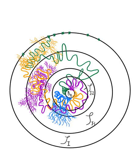
Figure 2: The Many Spines.

Proof.

The formal proof follows very much the picture we just presented. Define the event $E_{0}:=\{|\eta_{R_{I}}|\geq cR_{I}^{2}\},$ with $c$ as in Lemma 10.1. Let

$$E_{1}:=\big{\{}\sum_{u\in\eta_{R_{I}}}|\eta^{u}_{r/2}|>0\big{\}}.$$

Conditionally on $E_{1}$, we know by Proposition (3.3) that there exists a path (or spine), which we denote by $\Gamma_{1}=(\Gamma_{1}(i),\ 0\leq i\leq|\Gamma_{1}|)$, emanating from one of the points in $\{S_{u},u\in\eta_{R_{I}}\}$, and going up to $\partial B_{r/2}$. For $1\leq j\leq I$, and a path $\gamma$, we let

$$\tau_{j}=\tau_{j}(\gamma):=\inf\big{\{}k\geq 0:\gamma(k)\in\partial\mathcal{S}_{j}\big{\}}.$$

We then define $E_{2}$ as the event that one of the biased BRWs starting from the points in the path $\{\Gamma_{1}(i),\ 0\leq i<\tau_{I-1}\}$, hits $\partial B_{r/2}$. Applying Proposition (3.3) again, it means that on the event $E_{1}\cap E_{2}$ there exists a second spine $\Gamma_{2}$ emanating from one of the (neighbors of the) points in $\{\Gamma_{1}(i),\ 0\leq i<\tau_{I-1}\}$, going up to $\partial B_{r/2}$. We can thus define $E_{3}$ as the event that one of the biased BRWs starting from the points in $\{\Gamma_{1}(i),\ \tau_{I-1}\leq i<\tau_{I-2}\}\cup\{\Gamma_{2}(i),\ 0\leq i<\tau_{I-2}\}$, hits $\partial B_{r/2}$. Continuing like this in all the shells $\mathcal{S}_{I},\dots,\mathcal{S}_{I/2}$, we define inductively for each $i=1,\dots,I/2$, an event $E_{i}$, such that on $E_{1}\cap\dots\cap E_{i}$, there are $i$ spines $\Gamma_{1},\dots,\Gamma_{i}$, starting respectively from a point in $\partial B_{R_{I}},\partial\mathcal{S}_{I},\dots,\partial\mathcal{S}_{I-i+2}$, and going up to $\partial B_{r/2}$. We claim that there exists a constant $\rho>0$, such that for each $i\leq I/2$,

$$\mathbb{P}(E_{i+1}\mid E_{1}\cap\dots\cap E_{i})\geq\frac{\rho i}{I}.$$ (10.4)

Indeed, recall that by Corollary 3.4 the spines satisfy the strong Markov property. Therefore, for any $i$,

$$\mathbb{P}(E_{i+1}\mid E_{1}\cap\dots\cap E_{i})\geq 1-\big{(}1-\inf_{x\in\partial B_{R_{I-i+1}}}r_{i}(x)\big{)}^{i},$$

where for any $x\in\partial B_{R_{I-i+1}}$, we denote by $r_{i}(x)$ the probability that on a path $\Gamma$ starting from $x$, and sampled according to the measure $\mathbb{P}^{x}_{\partial B_{r/2}}$, one of the biased BRW starting from the points in $\{\Gamma(k),\ k\leq\tau_{I-i}\}$, hits $\partial B_{r/2}$. Since for any $z\in\mathcal{S}_{I-i+1}$ the probability to hit $\partial B_{r/2}$ is of order $I^{-1}\cdot R_{I-i}^{-2}$ (recall that we assume $i\leq I/2$), by Lemma 3.5 (which holds as well for a biased BRW), one has for some constant $c>0$, and any $\alpha>0$

$$r_{i}(x)\geq\Big{\{}1-\big{(}1-\frac{c}{IR_{I-i}^{2}}\big{)}^{\alpha R_{I-i}^{2}}\Big{\}}\cdot\mathbb{P}_{\partial B_{r/2}}^{x}\big{(}\ell_{\Gamma}(\mathcal{S}_{I-i+1})>\alpha R_{I-i}^{2}\big{)},$$

where for $j\geq 2$, we write $\ell_{\gamma}(\mathcal{S}_{j})$ for the time spent on $\mathcal{S}_{j}$ by a path $\gamma$, before its hitting time of $B_{R_{j-1}}$. Thus, to conclude the proof of (10.4), it suffices to show that for some $\alpha>0$, one has for any $j\geq 2$, and any $x\in\partial B_{R_{j}}$,

$$\mathbb{P}_{\partial B_{r/2}}^{x}\big{(}\ell_{\Gamma}(\mathcal{S}_{j})>\alpha R_{j}^{2}\big{)}\geq\alpha.$$ (10.5)

Set now $\Lambda:=\partial B_{r/2}$ to simplify notation. One has by definition of $\mathbb{P}_{\Lambda}^{x}$, and using also (3.4),

$$\mathbb{P}_{\Lambda}^{x}\big{(}\ell_{\Gamma}(\mathcal{S}_{j})\leq\alpha R_{j}^{2}\big{)} =\frac{\sum_{y\in\partial B_{R_{j-1}}}\left(\sum_{\gamma_{1}:x\to y}{\text{\Large$\mathfrak{1}$}}\{\ell_{\gamma}(\mathcal{S}_{j})\leq\alpha R_{j}^{2}\}p_{\Lambda}(\gamma_{1})\right)\cdot\left(\sum_{\gamma_{2}:y\to\Lambda}p_{\Lambda}(\gamma_{2})\right)}{\sum_{y\in\partial B_{R_{j-1}}}\left(\sum_{\gamma_{1}:x\to y}p_{\Lambda}(\gamma_{1})\right)\cdot\left(\sum_{\gamma_{2}:y\to\Lambda}p_{\Lambda}(\gamma_{2})\right)}$$

$$=\frac{\sum_{y\in\partial B_{R_{j-1}}}\left(\sum_{\gamma_{1}:x\to y}{\text{\Large$\mathfrak{1}$}}\{\ell_{\gamma_{1}}(\mathcal{S}_{j})\leq\alpha R_{j}^{2}\}p_{\Lambda}(\gamma_{1})\right)\cdot\mathbb{P}_{y}(|\eta_{r/2}|>0)}{\sum_{y\in\partial B_{R_{j-1}}}\left(\sum_{\gamma_{1}:x\to y}p_{\Lambda}(\gamma_{1})\right)\cdot\mathbb{P}_{y}(|\eta_{r/2}|>0)}$$

$$\leq C\frac{\sum_{y\in\partial B_{R_{j-1}}}\sum_{\gamma_{1}:x\to y}{\text{\Large$\mathfrak{1}$}}\{\ell_{\gamma_{1}}(\mathcal{S}_{j})\leq\alpha R_{j}^{2}\}p_{\Lambda}(\gamma_{1})}{\sum_{y\in\partial B_{R_{j-1}}}\sum_{\gamma_{1}:x\to y}p_{\Lambda}(\gamma_{1})},$$

for some constant $C>0$, using Lemma 3.5 and Proposition 3.11 for the last inequality. By (3.4), one has

$$\sum_{y\in\partial B_{R_{j-1}}}\ \sum_{\begin{subarray}{c}\gamma_{1}:x\to y\\ \ell_{\gamma_{1}}(\mathcal{S}_{j})\leq\alpha R_{j}^{2}\end{subarray}}p_{\Lambda}(\gamma_{1})\leq\sum_{y\in\partial B_{R_{j-1}}}\mathbf{P}_{x}\big{(}\ell_{S}(\mathcal{S}_{j})\leq\alpha R_{j}^{2},\,S_{\tau_{j-1}}=y\big{)}=\mathbf{P}_{x}\big{(}\ell_{S}(\mathcal{S}_{j})\leq\alpha R_{j}^{2},\,\tau_{j-1}<\infty\big{)},$$

while using also Proposition 3.11, we get that for some constant $c>0$,

$$\sum_{y\in\partial B_{R_{j-1}}}\sum_{\gamma_{1}:x\to y}p_{\Lambda}(\gamma_{1})\geq\sum_{y\in\partial B_{R_{j-1}}}\ \sum_{\begin{subarray}{c}\gamma_{1}:x\to y\\ |\gamma_{1}|\leq R_{j}^{2}\end{subarray}}p_{\Lambda}(\gamma_{1})\geq c\mathbf{P}_{x}\big{(}\tau_{j-1}(S)\leq R_{j}^{2})\geq c^{2}.$$

Now for any $\varepsilon>0$, one can find $\alpha$ small enough, such that

$$\mathbf{P}_{x}\big{(}\ell_{S}(\mathcal{S}_{j})\leq\alpha R_{j}^{2},\,\tau_{j-1}<\infty\big{)}\leq\mathbf{P}_{x}\big{(}\ell_{S}(\mathcal{S}_{j})\leq\alpha R_{j}^{2}\big{)}\leq\varepsilon.$$

Altogether this proves (10.5), and thus also (10.4). It follows that for some constant $\kappa>0$,

$$\mathbb{P}(E_{0}\cap\dots\cap E_{I/2})\geq\exp(-\kappa I).$$ (10.6)

We observe finally that on the event in the probability above, the number of particles which hit $\partial B_{r/2}$ dominates the sum of $I/2$ independent random variables $X_{1},\dots,X_{I/2}$ distributed as $|\eta_{r/2}|$, under the conditional law $\mathbb{P}_{z}(\cdot\mid|\eta_{r/2}|>0)$, for some $z\in\partial B_{R_{I/2}}$. However, for any such starting point $z$, one has using the computation made in the proof of Lemma 3.5, together with Proposition 3.11,

$$\mathbb{E}_{z}\big{[}|\eta_{r/2}|\mid|\eta_{r/2}|\neq 0\big{]}\gtrsim Ir^{2},\quad\text{and}\quad\mathbb{E}_{z}\big{[}|\eta_{r/2}|^{2}\mid|\eta_{r/2}|>0\big{]}\lesssim r^{4}I^{2}.$$

Thus Paley–Zygmund’s inequality (2.7) (applied to the law of $X_{1}+\dots+X_{I/2}$) gives the existence of $\alpha>0$, such that

$$\mathbb{P}\big{(}X_{1}+\dots+X_{I/2}\geq\alpha I^{2}r^{2}\big{)}\geq\alpha.$$

In other words, we just have proved that

$$\mathbb{P}\big{(}\sum_{u\in\eta_{R_{I}}}|\eta^{u}_{r/2}|\geq\alpha r^{2}I^{2}\big{)}\geq\frac{c}{r^{2}}\exp(-\kappa I),$$

for some positive constants $c$ and $\kappa$. The proof is now almost finished. To conclude, note that

$$\inf_{x\in B_{r/2}}\mathbb{E}_{x}\big{[}|\mathcal{T}(B_{r})|\big{]}=\inf_{x\in B_{r/2}}\mathbf{E}_{x}[H_{r}]\gtrsim r^{2},$$

and by definition,

$$\ell_{\mathcal{T}}(B_{r})\geq\sum_{u\in\eta_{R_{I}}}\sum_{v\in\eta^{u}_{r/2}}|\mathcal{T}^{v}(B_{r})|.$$

Thus by an application of the weak law of large numbers, and by taking the constant $C$ in the definition of $I$ large enough, we deduce

$$\mathbb{P}(\ell_{\mathcal{T}}(B_{r})>t)\geq\frac{c}{r^{2}}\exp(-\kappa I),$$

for some (possibly different) positive constants $c$ and $\kappa$. This concludes the proof of the lower bound in Theorem 1.1, in dimension four. $\square$

Acknowledgements. We would like to thank Ofer Zeitouni for many stimulating and enthusiastic discussions at an early stage of this work.

References

- [AS20b] A. Asselah, B. Schapira. Extracting subsets maximizing capacity and folding of random walks. To appear in Ann. Sc. de l’E.N.S. (2023).
- [AHJ21] O. Angel, T. Hutchcroft, A. Járai. On the tail of the branching random walk local time. Probab. Theory Related Fields 180 (2021), 467–494.
- [AN72] K. B. Athreya, P. E. Ney. Branching processes. Reprint of the 1972 original. Dover Publications, Inc., Mineola, NY, 2004. xii+287 pp.
- [BW20] T. Bai, Y. Wan. Capacity of the range of tree-indexed random walk, to appear in Ann. Appl. Probab. arXiv:2004.06018.
- [BH21] T. Bai, Y. Hu. Capacity of the range of branching random walks in low dimensions, to appear in Proc. Steklov Inst. Math., arXiv:2104.11898.
- [BH22] T. Bai, Y. Hu. Convergence in law for the capacity of the range of a critical branching random walk. arXiv:2203.03188.
- [BC12] I. Benjamini, N. Curien. Recurrence of the -valued infinite snake via unimodularity. Electron. Commun. Probab. 17 (2012), 10 pp.
- [DV75] M. D. Donsker; S. R. S. Varadhan. Asymptotics for the Wiener Sausage. Comm. Pure Appl. Math. 28 (1975), 525–565
- [DKLT] T. Duquesne, R. Khanfir, S. Lin, N. Torri. Scaling limits of tree-valued branching random walks, Electron. J. Probab., Vol. 27, (2022), 1–54.
- [DE51] A. Dvoretzky, P. Erdös. Some problems on random walk in space. Proceedings Second Berkeley Symposium on Math. Statistics and Probability, 353–367. University of California Press, Berkeley (1951). . Probab. Theory Related Fields 148 (2010), 527–566.
- [LZ11] S. P. Lalley, X. Zheng. Occupation statistics of critical branching random walks in two or higher dimensions. Ann. Probab. 39 (2011), 327–368.
- [LL10] G. F. Lawler; V. Limic. Random walk: a modern introduction. Cambridge Studies in Advanced Mathematics, 123. Cambridge University Press, Cambridge, 2010.
- [LGL15] J.-F. Le Gall, S. Lin. The range of tree-indexed random walk in low dimensions. Ann. Probab. 43 (2015), 2701–2728.
- [LGL16] J.-F. Le Gall, S. Lin. The range of tree-indexed random walk. J. Inst. Math. Jussieu 15 (2016), 271–317.
- [NV75] S. V. Nagaev, N. V. Vahrusev. An estimate of large deviation probabilities for a critical Galton-Watson process. (Russian) Teor. Verojatnost. i Primenen. 20 (1975), 181–182.
- [NV03] S. V. Nagaev, V. I. Vakhtel. Limit theorems for probabilities of large deviations of a Galton-Watson process. (Russian) Diskret. Mat. 15 (2003), no. 1, 3–27; translation in Discrete Math. Appl. 13 (2003), no. 1, 1–26
- [PZ19] E. B. Procaccia, Y. Zhang. Connectivity properties of Branching Interlacements. ALEA (2019).
- [Shi12] Z. Shi. Branching random walks. Lecture notes from the 42nd Probability Summer School held in Saint Flour, 2012. Lecture Notes in Mathematics, 2151. École d’Été de Probabilités de Saint-Flour. [Saint-Flour Probability Summer School] Springer, Cham, 2015. x+133 pp.
- [Zhu16a] Q. Zhu. On the critical branching random walk I: branching capacity and visiting probability, arXiv:1611.10324,
- [Zhu16b] Q. Zhu. On the critical branching random walk II: branching capacity and branching recurrence, arXiv:1612.00161
- [Zhu21] Q. Zhu. On the critical branching random walk III: The critical dimension. Ann. Inst. Henri Poincaré Probab. Stat. 57 (2021), 73–93.
- [Zhu19] Q. Zhu. An upper bound for the probability of visiting a distant point by a critical branching random walk in . Electron. Commun. Probab. 24 (2019), Paper No. 32, 6 pp.
- [Zhu18] Q. Zhu. Branching interlacements and tree-indexed random walks in tori. arXiv:1812.10858.