Walsh’s conformal map onto lemniscatic domains for polynomial pre-images I

Abstract

We consider Walsh’s conformal map from the exterior of a compact set $E\subseteq\mathbb{C}$ onto a lemniscatic domain. If $E$ is simply connected, the lemniscatic domain is the exterior of a circle, while if $E$ has several components, the lemniscatic domain is the exterior of a generalized lemniscate and is determined by the logarithmic capacity of $E$ and by the exponents and centers of the generalized lemniscate. For general $E$, we characterize the exponents in terms of the Green’s function of $E^{c}$. Under additional symmetry conditions on $E$, we also locate the centers of the lemniscatic domain. For polynomial pre-images $E=P^{-1}(\Omega)$ of a simply-connected infinite compact set $\Omega$, we explicitly determine the exponents in the lemniscatic domain and derive a set of equations to determine the centers of the lemniscatic domain. Finally, we present several examples where we explicitly obtain the exponents and centers of the lemniscatic domain, as well as the conformal map.

Keywords:

conformal map, lemniscatic domain, multiply connected domain, polynomial pre-image, Green’s function, logarithmic capacity

AMS Subject Classification (2020):

30C35; 30C20.

1 Introduction

The famous Riemann mapping theorem says that for any simply connected, compact and infinite set $E$ there exists a conformal map $\operatorname{\mathcal{R}}_{E}:E^{c}\coloneq\widehat{\mathbb{C}}\setminus E\to\overline{\mathbb{D}}^{c}$, where $\widehat{\mathbb{C}}=\mathbb{C}\cup\{\infty\}$ denotes the extended complex plane, $\mathbb{D}$ the open and $\overline{\mathbb{D}}$ the closed unit disk. By imposing the normalization $\operatorname{\mathcal{R}}_{E}(z)=\frac{z}{\operatorname{cap}(E)}+\mathcal{O}(1)$ as $z\to\infty$, where $\operatorname{cap}(E)$ denotes the logarithmic capacity of $E$, this map is unique. In his 1956 article [13], J. L. Walsh found the following canonical generalization for multiply connected domains.

Theorem 1.1.

Let $E_{1},\ldots,E_{\ell}\subseteq\mathbb{C}$ be disjoint simply connected, infinite compact sets and let

$$E=\bigcup_{j=1}^{\ell}E_{j}.$$ (1.1)

In particular, $E^{c}=\widehat{\mathbb{C}}\setminus E$ is an $\ell$-connected domain. Then there exists a unique compact set of the form

$$L\coloneq\{w\in\mathbb{C}:\lvert U(w)\rvert\leq\operatorname{cap}(E)\},\quad U(w)\coloneq\prod_{j=1}^{\ell}(w-a_{j})^{m_{j}},$$ (1.2)

where $a_{1},\ldots,a_{\ell}\in\mathbb{C}$ are distinct and $m_{1},\ldots,m_{\ell}>0$ are real numbers with $\sum_{j=1}^{\ell}m_{j}=1$, and a unique conformal map

$$\Phi:E^{c}\to L^{c}$$ (1.3)

normalized by

$$\Phi(z)=z+\mathcal{O}(1/z)\quad\text{at }\infty.$$ (1.4)

If $E$ is bounded by Jordan curves, then $\Phi$ extends to a homeomorphism from $\overline{E^{c}}$ to $\overline{L^{c}}$.

Remark 1.2.

1. By assumption, each $E_{j}$ satisfies $\operatorname{cap}(E_{j})>0$ hence $\operatorname{cap}(E)>0$.

2. The points $a_{1},\ldots,a_{\ell}$ (sometimes called ‘centers’ of $L$) and also $m_{1},\ldots,m_{\ell}$ in Theorem 1.1 are uniquely determined. The function $U$ is analytic in $\mathbb{C}\setminus\{a_{1},\ldots,a_{\ell}\}$ and in general not single-valued, but its absolute value is single-valued. Note that the compact set $L$, defined in (1.2), consists of $\ell$ disjoint compact components $L_{1},\ldots,L_{\ell}$, with $a_{j}\in L_{j}$ for $j=1,\ldots,\ell$. The components $L_{1},\ldots,L_{\ell}$ are labeled such that a Jordan curve surrounding $E_{j}$ is mapped by $\Phi$ onto a Jordan curve surrounding $L_{j}$.

3. If $E$ is simply connected then the exterior Riemann map $\operatorname{\mathcal{R}}_{E}:E^{c}\to\overline{\mathbb{D}}^{c}$ with $\operatorname{\mathcal{R}}_{E}(z)=d_{1}z+d_{0}+\mathcal{O}(1/z)$ at $\infty$ and $d_{1}=\operatorname{\mathcal{R}}_{E}^{\prime}(\infty)>0$ and the Walsh map $\Phi$ are related by $\operatorname{\mathcal{R}}_{E}(z)=d_{1}\Phi(z)+d_{0}$, which follows from [13, Thm. 4]. The corresponding lemniscatic domain is the disk $L=\{w\in\mathbb{C}:\lvert w-a_{1}\rvert\leq\operatorname{cap}(E)\}$, where $a_{1}=-d_{0}/d_{1}$ and $\operatorname{cap}(E)=1/d_{1}$. This shows that Walsh’s map onto lemniscatic domains is a canonical generalization of the Riemann map from simply to multiply connected domains.

4. The existence in Theorem 1.1 was first shown by Walsh; see [13, Thm. 3] and the discussion below. Other existence proofs were given by Grunsky [2], [3], and [4, Thm. 3.8.3], and also by Jenkins [5] and Landau [6]. However, these articles do not contain any analytic or numerical examples. The first analytic examples were constructed by Sète and Liesen in [12], and, subsequently, a numerical method for computing the Walsh map was derived in [8] for sets bounded by smooth Jordan curves.

5. The domain $L^{c}$ is usually called a lemniscatic domain. This term seems to originate in Grunsky [4, p. 106].

In this paper, we bring some light into the computation of the parameters $m_{j}$ and $a_{j}$ appearing in Theorem 1.1.

In Section 2, as a first main result, we derive a general formula (Theorem 2.3) for the exponents $m_{j}$ in terms of the Green’s function of $E^{c}$, denoted by $g_{E}$. Of special interest is of course the case when $E$ is real or when $E$ or some component $E_{j}$ are symmetric with respect to the real line, i.e., $E^{*}=E$ or $E_{j}^{*}=E_{j}$, where

$$K^{*}\coloneq\{z\in\widehat{\mathbb{C}}:\overline{z}\in K\}$$ (1.5)

denotes the complex conjugate of a set $K\subseteq\widehat{\mathbb{C}}$. We prove that $E^{*}=E$ and $E_{j}^{*}=E_{j}$ implies that $a_{j}\in\mathbb{R}$ (Theorem 2.7). In the case that all components are symmetric, we give an interlacing property of the components $E_{j}$ and the critical points of $g_{E}$ (Theorem 2.8).

In Section 3, we consider the case when $E$ is a polynomial pre-image of a simply connected compact infinite set $\Omega$, that is, $E=P_{n}^{-1}(\Omega)$. In this case, we prove in Theorem 3.2 that the $m_{j}$ are always rational of the form $m_{j}=n_{j}/n$, where $n$ is the degree of the polynomial $P_{n}$ and $n_{j}$ is the number of zeros of $P_{n}(z)-\omega$ in $E_{j}$, where $\omega\in\Omega$. Moreover, the unknowns $a_{1},\ldots,a_{\ell}$ are characterized by a system of equations which in particular can be solved explicitly in the case $\ell=2$. With the help of these findings, we obtain an analytic expression for the map $\Phi$ if $P_{n}^{-1}(\Omega)$ is connected (Corrolary 3.7).

Finally, Section 4 contains several illustrative examples when $E=P_{n}^{-1}(\Omega)$ and when $\Omega=\overline{\mathbb{D}}$, $\Omega=[-1,1]$ or when $\Omega$ is a Chebyshev ellipse. In particular, we determine the exponents and centers of the corresponding lemniscatic domain and visualize the conformal map $\Phi$.

2 Results for general compact sets

Let the notation be as in Theorem 1.1. The Green’s function (with pole at $\infty$) of $L^{c}$ is

$$g_{L}(w)=\log\lvert U(w)\rvert-\log(\operatorname{cap}(E))=\sum_{j=1}^{\ell}m_{j}\log\lvert w-a_{j}\rvert-\log(\operatorname{cap}(E))$$ (2.1)

since $g_{L}$ is harmonic in $\mathbb{C}\setminus\{a_{1},\ldots,a_{\ell}\}$, is zero on $\partial(L^{c})$, and $g_{L}(w)-\log\lvert w\rvert$ is harmonic at $\infty$ with $\lim_{w\to\infty}(g_{L}(w)-\log\lvert w\rvert)=-\log(\operatorname{cap}(E))$. Then the Green’s function of $E^{c}$ is

$$g_{E}(z)=g_{L}(\Phi(z)),\quad z\in E^{c},$$ (2.2)

since $\Phi:E^{c}\to L^{c}$ is conformal with $\Phi(z)=z+\mathcal{O}(1/z)$ at $\infty$. In particular, $\operatorname{cap}(E)=\operatorname{cap}(L)$. Denote for $R>1$ the level curves of $g_{E}$ and $g_{L}$ by

$$\Gamma_{R}=\{z\in E^{c}:g(z)=\log(R)\},\quad\Lambda_{R}=\{w\in L^{c}:g_{L}(w)=\log(R)\}.$$

Then $\Phi(\Gamma_{R})=\Lambda_{R}$ and $\Phi$ maps the exterior of $\Gamma_{R}$ onto the exterior of $\Lambda_{R}$. Let $R_{*}>1$ be the largest number, such that $g_{E}$ has no critical point interior to $\Gamma_{R_{*}}$ (if $\ell=1$, then $R_{*}=\infty$; see Theorem 2.5 below). Then $\Phi$ is the conformal map of $\operatorname{ext}(\Gamma_{R})$ onto the lemniscatic domain $\operatorname{ext}(\Lambda_{R})$ for all $1<R<R_{*}$; see also [14, p. 31].

Here and in the following, we extensively use the Wirtinger derivatives

$$\partial_{z}=\frac{1}{2}(\partial_{x}-i\partial_{y})\quad\text{and}\quad\partial_{\overline{z}}=\frac{1}{2}(\partial_{x}+i\partial_{y}),$$

where $z=x+iy$ with $x,y\in\mathbb{R}$. We relate the exponents and centers of the lemniscatic domain to the Wirtinger derivatives $\partial_{z}g_{E}$ and $\partial_{w}g_{L}$ of the Green’s functions. Note that $\partial_{z}g$ is analytic if $g$ is a harmonic function, since then $\partial_{\overline{z}}(\partial_{z}g)=\frac{1}{4}\Delta g=0$.

Lemma 2.1.

The Green’s functions $g_{L}$ and $g_{E}$ from (2.1) and (2.2) satisfy

$$\partial_{z}g_{E}(z)=\partial_{w}g_{L}(\Phi(z))\cdot\Phi^{\prime}(z).$$ (2.3)

Moreover, if $\gamma:[a,b]\to E^{c}$ is a smooth path, then

$$\int_{\gamma}\partial_{z}g_{E}(z)\,dz=\int_{\Phi\circ\gamma}\partial_{w}g_{L}(w)\,dw.$$ (2.4)

Proof.

Since $\Phi$ is analytic, we have $\partial_{z}\Phi=\Phi^{\prime}$ and $\partial_{\overline{z}}\Phi=0$. Moreover, $\partial_{z}\overline{\Phi}=\overline{\partial_{\overline{z}}\Phi}=0$. With the chain rule for the Wirtinger derivatives and (2.2), we find

$$\frac{\partial g_{E}}{\partial z}(z)=\frac{\partial g_{L}}{\partial w}(\Phi(z))\cdot\frac{\partial\Phi}{\partial z}(z)+\frac{\partial g_{L}}{\partial\overline{w}}(\Phi(z))\cdot\frac{\partial\overline{\Phi}}{\partial z}(z)=\partial_{w}g_{L}(\Phi(z))\cdot\Phi^{\prime}(z),$$ (2.5)

which is (2.3). Integrating this expression over $\gamma$ yields

$$\int_{\gamma}\partial_{w}g_{L}(\Phi(z))\Phi^{\prime}(z)\,dz=\int_{a}^{b}\partial_{w}g_{L}(\Phi(\gamma(t)))\Phi^{\prime}(\gamma(t))\gamma^{\prime}(t)\,dt=\int_{\Phi\circ\gamma}\partial_{w}g_{L}(w)\,dw.$$ (2.6)

In combination with (2.3), this yields (2.4). ∎

Remark 2.2.

Formally, equation (2.3) yields the relation between differentials

$$\partial_{z}g_{E}(z)\,dz=\partial_{w}g_{L}(\Phi(z))\cdot\Phi^{\prime}(z)\,dz=\partial_{w}g_{L}(w)\,dw,$$ (2.7)

which yields (2.4) upon integrating.

We are now ready to express the exponents $m_{j}$ through the Wirtinger derivatives of the Green’s function. For $j=1,\ldots,\ell$, let $\gamma_{j}$ be a closed curve in $\mathbb{C}\setminus E$ with $\operatorname{wind}(\gamma_{j};z)=\delta_{jk}$ for $z\in E_{k}$ and $k=1,\ldots,\ell$, where $\operatorname{wind}(\gamma;z_{0})$ denotes the winding number of the curve $\gamma$ about $z_{0}$, and $\delta_{jk}$ is the usual Kronecker delta. More informally, the curve $\gamma_{j}$ contains $E_{j}$ but no $E_{k}$, $k\neq j$, in its interior.

Theorem 2.3.

In the notation of Theorem 1.1, let $g_{E}$ and $g_{L}$ be the Green’s functions of $E^{c}$ and $L^{c}$, respectively. For each $j\in\{1,\ldots,\ell\}$, let $\gamma_{j}$ be a closed curve in $\mathbb{C}\setminus E$ with $\operatorname{wind}(\gamma_{j};z)=\delta_{jk}$ for $z\in E_{k}$ and $k=1,\ldots,\ell$, and let $\lambda_{j}=\Phi\circ\gamma_{j}$. Then,

$$m_{j}=\frac{1}{2\pi i}\int_{\lambda_{j}}2\partial_{w}g_{L}(w)\,dw=\frac{1}{2\pi i}\int_{\gamma_{j}}2\partial_{z}g_{E}(z)\,dz.$$ (2.8)

Moreover, if the function $f$ is analytic interior to $\lambda_{j}$ and continuous on $\operatorname{trace}(\lambda_{j})$, then

$$m_{j}f(a_{j})=\frac{1}{2\pi i}\int_{\lambda_{j}}f(w)2\partial_{w}g_{L}(w)\,dw=\frac{1}{2\pi i}\int_{\gamma_{j}}f(\Phi(z))2\partial_{z}g_{E}(z)\,dz.$$ (2.9)

Proof.

Since $2\partial_{w}\log\lvert w\rvert=\partial_{w}\log(w\overline{w})=1/w$, we obtain from (2.1) that

$$2\partial_{w}g_{L}(w)=\sum_{j=1}^{\ell}\frac{m_{j}}{w-a_{j}},$$ (2.10)

which is a rational function. By construction, $\lambda_{j}$ is a closed curve in $\mathbb{C}\setminus L$ with $\operatorname{wind}(\lambda_{j};a_{k})=\delta_{jk}$. Integrating over $\lambda_{j}$ yields the first equality in (2.8). The second equality follows by Lemma 2.1. Using (2.10) and the residue theorem, we obtain

$$\frac{1}{2\pi i}\int_{\lambda_{j}}f(w)2\partial_{w}g_{L}(w)\,dw=\frac{1}{2\pi i}\int_{\lambda_{j}}\sum_{s=1}^{\ell}\frac{m_{s}f(w)}{w-a_{s}}\,dw=m_{j}f(a_{j}).$$ (2.11)

This shows the first equality in (2.9). Multiplying (2.3) by $f(\Phi(z))$ and integrating yields the second equality in (2.9). ∎

Remark 2.4.

1. By (2.8) in Theorem 2.3, the exponent $m_{j}$ of the lemniscatic domain is the residue of $2\partial_{w}g_{L}$ at $a_{j}$. Moreover, $m_{j}$ is (up to the factor $\frac{1}{2\pi i}$) the module of periodicity (or period) of the differential $2\partial_{z}g_{E}(z)\,dz$; see [1, p. 147]. The latter can be rewritten as

   $$\int_{\gamma_{j}}2\partial_{z}g_{E}(z)\,dz=\int_{\gamma_{j}}\left(-\frac{\partial g_{E}}{\partial y}dx+\frac{\partial g_{E}}{\partial x}dy\right)=\int_{\gamma_{j}}\frac{\partial g_{E}}{\partial n}(z)\,\lvert dz\rvert,$$

   where the middle integral is over the conjugate differential of $dg_{E}$, and where $\frac{\partial g_{E}}{\partial n}$ is the derivative with respect to the normal pointing to the right of $\gamma_{j}$; see [1, pp. 162–164] for a detailed discussion.

2. Since $\partial_{z}g_{E}$ is analytic in $E^{c}$ and $\partial_{w}g_{L}$ is analytic in $\widehat{\mathbb{C}}\setminus\{a_{1},\ldots,a_{\ell}\}\supseteq L^{c}$, the integrals in (2.8) have the same value for all positively oriented closed curves that contain only $E_{j}$ or $a_{j}$ in their interior.

The following well-known result due to J. L. Walsh [15] establishes a relation between the critical points of the Green’s function and the connectivity of $E^{c}$.

Theorem 2.5 ([15, pp. 67–68]).

Let $E\subseteq\mathbb{C}$ be compact such that $\mathcal{K}=E^{c}$ is connected and such that $\mathcal{K}$ possesses a Green’s function $g_{E}$ with pole at infinity. If $\mathcal{K}$ is of finite connectivity $\ell$, then $g_{E}$ has precisely $\ell-1$ critical points in $\mathbb{C}\setminus E$, counted according to their multiplicity. If $\mathcal{K}$ is of infinite connectivity, $g_{E}$ has a countably infinite number of critical points. Moreover, all critical points of $g_{E}$ lie in the convex hull of $E$.

As is typical for conformal maps with $\Phi(z)=z+\mathcal{O}(1/z)$ at $\infty$, symmetry of $E$ (e.g., rotational symmetry or symmetry with respect to the real line) leads to the same symmetry of $L$, and to “symmetry” in the map $\Phi$.

Lemma 2.6 ([12, Lem. 2.2]).

Let the notation be as in Theorem 1.1. Then the following symmetry relations hold.

1. If $E=E^{*}$, then $L=L^{*}$ and $\Phi(z)=\overline{\Phi(\overline{z})}$.

2. If $E=e^{i\theta}E\coloneq\{e^{i\theta}z:z\in E\}$, then $L=e^{i\theta}L$ and $\Phi(z)=e^{-i\theta}\Phi(e^{i\theta}z)$.

3. In particular: If $E=-E=\{-z:z\in E\}$, then $L=-L$ and $\Phi(z)=-\Phi(-z)$.

In the last two results of this section, we consider the case where $E$ and one or all of its components $E_{j}$ are symmetric with respect to the real line. This allows to locate the points $a_{1},\ldots,a_{\ell}$ and the critical points of the Green’s function $g_{E}$.

Theorem 2.7.

In the notation of Theorem 1.1, suppose that $E^{*}=E$. Let $j\in\{1,\ldots,\ell\}$. If $E_{j}^{*}=E_{j}$ then $a_{j}\in\mathbb{R}$.

Proof.

Since $E^{*}=E$, we have $\Phi(\overline{z})=\overline{\Phi(z)}$ by Lemma 2.6 and $\partial_{z}g_{E}(\overline{z})=\overline{\partial_{z}g_{E}(z)}$ by Lemma A.1. Next, if $E_{j}^{*}=E_{j}$ for some $j\in\{1,\ldots,\ell\}$ then there exists a smooth Jordan curve $\gamma_{j}$ in $\mathbb{C}\setminus E$ symmetric with respect to the real line which surrounds $E_{j}$ in the positive sense, but no other component $E_{k}$, $k\neq j$, i.e., $\operatorname{wind}(\gamma_{j};z)=\delta_{jk}$ for $z\in E_{k}$ and $k=1,\ldots,\ell$. By (2.9),

$$m_{j}a_{j}=\frac{1}{2\pi i}\int_{\gamma_{j}}\Phi(z)2\partial_{z}g_{E}(z)\,dz,$$

where $\Phi(\overline{z})2\partial_{z}g_{E}(\overline{z})=\overline{\Phi(z)2\partial_{z}g_{E}(z)}$ on $\gamma_{j}$. By Lemma A.3, we obtain $m_{j}a_{j}\in\mathbb{R}$, hence $a_{j}\in\mathbb{R}$ since $m_{j}>0$. ∎

In Theorem 2.7, if a component $E_{j}$ is not symmetric with respect to the real line, then the corresponding point $a_{j}$ is in general not real, as the example of the star in [12, Cor. 3.3] shows.

If $E_{j}^{*}=E_{j}$ for all components of $E$ then we order the components “from left to right”: By Lemma A.2, each $E_{j}\cap\mathbb{R}$ is a point or an interval, and we label $E_{1},\ldots,E_{\ell}$ such that $x\in E_{j}\cap\mathbb{R}$ and $y\in E_{j+1}\cap\mathbb{R}$ implies $x<y$ for all $j=1,\ldots,\ell-1$.

Theorem 2.8.

Let $E=E_{1}\cup\ldots\cup E_{\ell}$ be as in Theorem 1.1 and suppose that $E_{j}^{*}=E_{j}$ for all $j=1,\ldots,\ell$. Then the following hold.

1. The $\ell-1$ critical points of the Green’s function $g_{E}$ are real. Moreover, each $E_{j}$ intersects $\mathbb{R}$ in a point or an interval, and the critical points of $g_{E}$ interlace the sets $E_{j}\cap\mathbb{R}$, $j=1,\ldots,\ell$.

2. If $E_{1},\ldots,E_{\ell}$ are ordered “from left to right” then $a_{1}<a_{2}<\ldots<a_{\ell}$.

Proof.

(i) For each $j=1,\ldots,\ell$, the set $E_{j}\cap\mathbb{R}$ is a point or an interval by Lemma A.2. For $j=1,\ldots,\ell-1$, denote the ‘gap’ on the real line between $E_{j}$ and $E_{j+1}$ by

$$I_{j}\coloneq]\max(E_{j}\cap\mathbb{R}),\min(E_{j+1}\cap\mathbb{R})[,\quad j=1,\ldots,\ell-1.$$

The Green’s function $g_{E}$ is positive on $I_{j}$ and can be continuously extended to $\overline{I}_{j}$ with boundary values $0$. Then $g_{E}$ has a maximum on $\overline{I}_{j}$ at a point $x_{j}\in I_{j}$ at which $\partial_{x}g_{E}(x_{j})=0$. By (A.1), we have $\partial_{y}g_{E}(x_{j})=-\partial_{y}g_{E}(x_{j})$, i.e., $\partial_{y}g_{E}(x_{j})=0$. This shows that $x_{j}$ is a critical point of $g_{E}$ for $j=1,\ldots,\ell-1$. These are the $\ell-1$ critical points of $g_{E}$ which are real and interlace the sets $E_{j}\cap\mathbb{R}$.

(ii) Since $E=E^{*}$, we have $\Phi(z)=\overline{\Phi(\overline{z})}$ by Lemma 2.6. In particular, $\Phi$ maps $\mathbb{R}\setminus E$ onto $\mathbb{R}\setminus L$. Since $\Phi(z)=z+\mathcal{O}(1/z)$ at infinity, $\Phi$ maps $I_{0}\coloneq]-\infty,\min(E_{1}\cap\mathbb{R})[$ onto $J_{0}\coloneq]-\infty,\min(L\cap\mathbb{R})[$. Let $\gamma_{1}$ be a Jordan curve in $\mathbb{C}\setminus E$ which surrounds $E_{1}$ in the positive sense, but no other component $E_{k}$, $k\neq 1$. Then $\gamma_{1}$ intersects $I_{0}$ and $I_{1}$ (see (i)), hence the curve $\Phi(\gamma_{1})$ intersects the images $J_{0}=\Phi(I_{0})$ and $J_{1}\coloneq\Phi(I_{1})$. This shows that $L_{1}$ is the leftmost component of $L$ and $a_{1}$ is the minimum of $a_{1},\ldots,a_{\ell}$. Proceeding in a similar way gives that the components $L_{1},\ldots,L_{\ell}$ are ordered from left to right, and therefore $a_{1}<a_{2}<\ldots<a_{\ell}$. ∎

3 Results for polynomial pre-images

Let $\Omega\subseteq\mathbb{C}$ be a compact infinite set such that $\Omega^{c}$ is a simply connected domain in $\widehat{\mathbb{C}}$ and let $\operatorname{\mathcal{R}}_{\Omega}$ be the exterior Riemann map of $\Omega$, i.e., the conformal map

$$\operatorname{\mathcal{R}}_{\Omega}:\Omega^{c}\to\overline{\mathbb{D}}^{c}\quad\text{with }\operatorname{\mathcal{R}}_{\Omega}(z)=d_{1}z+d_{0}+\sum_{k=1}^{\infty}\frac{d_{-k}}{z^{k}}\quad\text{for }\lvert z\rvert>R,$$ (3.1)

where

$$d_{1}=\operatorname{\mathcal{R}}_{\Omega}^{\prime}(\infty)=\frac{1}{\operatorname{cap}(\Omega)}>0,$$ (3.2)

$R\coloneq\max_{z\in\Omega}\lvert z\rvert$, and $\mathbb{D}=\{z\in\mathbb{C}:\lvert z\rvert<1\}$ is the open unit disk. By [9, Thm. 4.4.4], the Green’s function of $\Omega^{c}$ is

$$g_{\Omega}(z)=\log\lvert\operatorname{\mathcal{R}}_{\Omega}(z)\rvert.$$ (3.3)

Let $P_{n}$ be a polynomial of degree $n\geq 1$, more precisely,

$$P_{n}(z)=\sum_{j=0}^{n}p_{j}z^{j}\quad\text{with }p_{n}\in\mathbb{C}\setminus\{0\},$$ (3.4)

and consider the pre-image of $\Omega$ under $P_{n}$, that is

$$E=P_{n}^{-1}(\Omega)=\{z\in\mathbb{C}:P_{n}(z)\in\Omega\}.$$ (3.5)

The set $E$ is compact and, by Theorem A.4, the complement $E^{c}$ is connected. Therefore, the Green’s function of $E^{c}$ is

$$g_{E}(z)=\frac{1}{n}g_{\Omega}(P_{n}(z))=\frac{1}{n}\log\lvert\operatorname{\mathcal{R}}_{\Omega}(P_{n}(z))\rvert,$$ (3.6)

see [9, p. 134]. Since $2\partial_{z}\log\lvert f\rvert=f^{\prime}/f$ for an analytic function $f$, we have

$$2\partial_{z}g_{E}(z)=\frac{1}{n}\frac{\operatorname{\mathcal{R}}_{\Omega}^{\prime}(P_{n}(z))P_{n}^{\prime}(z)}{\operatorname{\mathcal{R}}_{\Omega}(P_{n}(z))}.$$ (3.7)

The logarithmic capacity of $E$ is

$$\operatorname{cap}(E)=\operatorname{cap}(P_{n}^{-1}(\Omega))=\left(\frac{\operatorname{cap}(\Omega)}{\lvert p_{n}\rvert}\right)^{1/n}=\frac{1}{\sqrt[n]{d_{1}\lvert p_{n}\rvert}},$$ (3.8)

see [9, Thm. 5.2.5].

By Theorem 2.5, the number of components of $E$ can be characterized as follows. For the case $\Omega=[-1,1]$, see also [10, Thm. 4 and Thm. 5].

Theorem 3.1.

The set $E$ in (3.5) consists of $\ell$ disjoint simply connected compact components $E_{1},\ldots,E_{\ell}$, i.e.,

$$E=P_{n}^{-1}(\Omega)=\bigcup_{j=1}^{\ell}E_{j},$$ (3.9)

if and only if $P_{n}$ has exactly $\ell-1$ critical points $z_{1},\ldots,z_{\ell-1}$ (counting multiplicities) for which $P_{n}(z_{k})\notin\Omega$ for $k=1,\ldots,\ell-1$. Moreover, the number of zeros of $P_{n}(z)-\omega$ in $E_{j}$ is the same for all $\omega\in\Omega$, and this number is denoted by $n_{j}$.

Proof.

By Theorem 2.5, $E$ has $\ell$ components if and only if $g_{E}$ has $\ell-1$ critical points (in $\mathbb{C}\setminus E$). Since $g_{E}$ is real-valued, $z_{0}\in\mathbb{C}\setminus E$ is a critical point of $g_{E}$ if and only if $\partial_{z}g_{E}(z_{0})=0$. By (3.7), the latter is equivalent to $P_{n}^{\prime}(z_{0})=0$.

For $j=1,\ldots,\ell$, let $\gamma_{j}$ be a Jordan curve in $\mathbb{C}\setminus E$ with $\operatorname{wind}(\gamma_{j};z)=\delta_{jk}$ for $z\in E_{k}$ and $k=1,\ldots,\ell$. Let $z_{0}\in E_{j}$ and $\omega_{0}\coloneq P_{n}(z_{0})\in\Omega$, then, by the argument principle,

$$n_{j}\coloneq\operatorname{wind}(P_{n}\circ\gamma_{j};\omega_{0})=\lvert\{z\in E_{j}:P_{n}(z)=\omega_{0}\}\rvert\geq 1.$$ (3.10)

Since $P_{n}\circ\gamma_{j}$ is a closed curve in $\mathbb{C}\setminus\Omega$, we have $\operatorname{wind}(P_{n}\circ\gamma_{j};\omega)=\operatorname{wind}(P_{n}\circ\gamma_{j};\omega_{0})$ for all $\omega\in\Omega$, i.e., every point in $\Omega$ has exactly $n_{j}$ pre-images under $P_{n}$ in $E_{j}$. ∎

In the rest of this section, we assume that $E$ has $\ell$ components $E_{1},\ldots,E_{\ell}$, i.e., that $P_{n}$ has exactly $\ell-1$ critical points with critical values in $\mathbb{C}\setminus\Omega$.

Theorem 3.2.

Let $E=P_{n}^{-1}(\Omega)$ and the numbers $n_{1},\ldots,n_{\ell}$ be defined as in Theorem 3.1. Then the exponents $m_{j}$ in the lemniscatic domain in Theorem 1.1 are given by

$$m_{j}=\frac{n_{j}}{n},\quad j=1,\ldots,\ell.$$ (3.11)

Proof.

For $j=1,\ldots,\ell$, let $\gamma_{j}$ be a positively oriented Jordan curve in $\mathbb{C}\setminus E$ with $\operatorname{wind}(\gamma_{j};z)=\delta_{jk}$ for $z\in E_{k}$ and $k=1,\ldots,\ell$. Using (2.8) and (3.7), we obtain

$$m_{j}=\frac{1}{2\pi i}\int_{\gamma_{j}}2\partial_{z}g_{E}(z)\,dz=\frac{1}{n}\frac{1}{2\pi i}\int_{\gamma_{j}}\frac{\operatorname{\mathcal{R}}_{\Omega}^{\prime}(P_{n}(z))P_{n}^{\prime}(z)}{\operatorname{\mathcal{R}}_{\Omega}(P_{n}(z))}\,dz.$$ (3.12)

Substituting $u=P_{n}(z)$ yields

$$m_{j}=\frac{1}{n}\frac{1}{2\pi i}\int_{P_{n}\circ\gamma_{j}}\frac{\operatorname{\mathcal{R}}_{\Omega}^{\prime}(u)}{\operatorname{\mathcal{R}}_{\Omega}(u)}\,du.$$ (3.13)

Since $\operatorname{wind}(P_{n}\circ\gamma_{j};u_{0})=n_{j}$ for $u_{0}\in\Omega$, the integral in (3.13) can be replaced by $n_{j}$ times an integral over a positively oriented Jordan curve $\Gamma$ in $\mathbb{C}\setminus\Omega$, i.e.,

$$m_{j}=\frac{n_{j}}{n}\frac{1}{2\pi i}\int_{\Gamma}\frac{\operatorname{\mathcal{R}}_{\Omega}^{\prime}(u)}{\operatorname{\mathcal{R}}_{\Omega}(u)}\,du.$$ (3.14)

The integral is

$$\frac{1}{2\pi i}\int_{\Gamma}\frac{\operatorname{\mathcal{R}}_{\Omega}^{\prime}(u)}{\operatorname{\mathcal{R}}_{\Omega}(u)}\,du=\frac{1}{2\pi i}\int_{\Gamma}\frac{\frac{(u-u_{0})\operatorname{\mathcal{R}}_{\Omega}^{\prime}(u)}{\operatorname{\mathcal{R}}_{\Omega}(u)}}{u-u_{0}}\,du=\lim_{u\to\infty}\frac{(u-u_{0})\operatorname{\mathcal{R}}_{\Omega}^{\prime}(u)}{\operatorname{\mathcal{R}}_{\Omega}(u)}=1$$ (3.15)

by Cauchy’s integral formula for an infinite domain; see, e.g., [7, Problem 14.14]. ∎

Next, we derive a relation between the Walsh map $\Phi$ and the Riemann map $\operatorname{\mathcal{R}}_{\Omega}$. Let $E=P_{n}^{-1}(\Omega)$ be as in (3.5). Liesen and the second author proved in [12, Eqn. (3.2)] that the lemniscatic map $\Phi$ in Theorem 1.1 and the exterior Riemann map $\operatorname{\mathcal{R}}_{\Omega}$ are related by

$$\lvert U(\Phi(z))\rvert=\operatorname{cap}(E)\lvert\operatorname{\mathcal{R}}_{\Omega}(P_{n}(z))\rvert^{1/n},\quad z\in E^{c},$$ (3.16)

with $U$ from (1.2). This follows by considering the identity (2.2) between the corresponding Green’s functions. In Theorem 3.3, we establish a stronger result.

By Theorem 3.2, the exponents of $U$ satisfy $m_{j}=n_{j}/n$. Together with (3.8), we see that

$$Q(w)\coloneq\frac{e^{i\arg(p_{n})}}{\operatorname{cap}(E)^{n}}U(w)^{n}=d_{1}p_{n}\prod_{j=1}^{\ell}(w-a_{j})^{n_{j}}$$ (3.17)

is a polynomial of degree $n$. Note that $L=\{w\in\mathbb{C}:\lvert Q(w)\rvert\leq 1\}$, and $Q:L^{c}\to\overline{\mathbb{D}}^{c}$ is an $n$-to-$1$ map. Then, equation (3.16) is equivalent to

$$\lvert Q(\Phi(z))\rvert=\lvert\operatorname{\mathcal{R}}_{\Omega}(P_{n}(z))\rvert,\quad z\in E^{c}.$$ (3.18)

Next, we show that equality is also valid without the absolute value. Moreover, we derive a relation between the points $a_{j}$ and the coefficients $p_{n-1}$, $p_{n}$ of $P_{n}$ for $n\geq 2$. The case $n=1$ is discussed in Remark 3.4.

Theorem 3.3.

Let $E=P_{n}^{-1}(\Omega)$ be as in (3.5). We then have

$$Q(\Phi(z))=\operatorname{\mathcal{R}}_{\Omega}(P_{n}(z)),\quad z\in E^{c},$$ (3.19)

that is,

$$\Phi=Q^{-1}\circ\operatorname{\mathcal{R}}_{\Omega}\circ P_{n},$$ (3.20)

with that branch of $Q^{-1}$ such that $\Phi(z)=z+\mathcal{O}(1/z)$ at $\infty$. Moreover, for $n\geq 2$,

$$\sum_{j=1}^{\ell}n_{j}a_{j}=-\frac{p_{n-1}}{p_{n}}.$$ (3.21)

Proof.

Consider the Laurent series at infinity of $\operatorname{\mathcal{R}}_{\Omega}\circ P_{n}$ and $Q\circ\Phi$. By (3.1) and (3.4),

$$\operatorname{\mathcal{R}}_{\Omega}(P_{n}(z))=d_{1}P_{n}(z)+d_{0}+\sum_{k=1}^{\infty}\frac{d_{-k}}{P_{n}(z)^{k}}=d_{1}p_{n}z^{n}+d_{1}p_{n-1}z^{n-1}+\mathcal{O}(z^{n-2}).$$ (3.22)

Since $\Phi(z)=z+\mathcal{O}(1/z)$ at infinity, we have

$$(\Phi(z)-a_{j})^{n_{j}}=(z-a_{j})^{n_{j}}+\mathcal{O}(z^{n_{j}-2})=z^{n_{j}}-n_{j}a_{j}z^{n_{j}-1}+\mathcal{O}(z^{n_{j}-2})$$

and, by (3.17),

$$Q(\Phi(z))=d_{1}p_{n}\prod_{j=1}^{\ell}(\Phi(z)-a_{j})^{n_{j}}=d_{1}p_{n}z^{n}-d_{1}p_{n}\sum_{j=1}^{\ell}n_{j}a_{j}z^{n-1}+\mathcal{O}(z^{n-2}).$$ (3.23)

The function $(Q\circ\Phi)/(\operatorname{\mathcal{R}}_{\Omega}\circ P_{n})$ is analytic in $\mathbb{C}\setminus E$ with constant modulus one, see (3.18), therefore constant (maximum modulus principle) and

$$Q(\Phi(z))=c\operatorname{\mathcal{R}}_{\Omega}(P_{n}(z)),\quad z\in E^{c},$$ (3.24)

where $c\in\mathbb{C}$ with $\lvert c\rvert=1$. By comparing the coefficients of $z^{n}$ of the Laurent series at $\infty$, we see that $c=1$, which shows (3.19). Comparing the coefficients of $z^{n-1}$ then yields (3.21). ∎

Figure 1: Commutative diagram of the maps in Theorem 3.3.

Figure 1 illustrates Theorem 3.3.

Remark 3.4.

In the case $n=1$, i.e., $P_{1}(z)=p_{1}z+p_{0}$ is a linear transformation, the conformal map and lemniscatic domain are given explicitly as follows. In this case, $E=P_{1}^{-1}(\Omega)$ consists of a single component, i.e., $\ell=1$ and $m_{1}=1$, and $Q(w)=d_{1}p_{1}(w-a_{1})$. Comparing the constant terms at infinity of $\operatorname{\mathcal{R}}_{\Omega}(P_{n}(z))=d_{1}p_{1}z+(d_{1}p_{0}+d_{0})+\mathcal{O}(1/z)$ with $Q(\Phi(z))$ from (3.23) yields

$$a_{1}=-\frac{d_{1}p_{0}+d_{0}}{d_{1}p_{1}}.$$ (3.25)

By Theorem 3.3, the conformal map $\Phi:E^{c}\to L^{c}$ is

$$\Phi(z)=(Q^{-1}\circ\operatorname{\mathcal{R}}_{\Omega}\circ P_{1})(z)=\frac{1}{d_{1}p_{1}}\operatorname{\mathcal{R}}_{\Omega}(p_{1}z+p_{0})+a_{1},$$ (3.26)

and

$$L=\left\{w\in\mathbb{C}:\lvert w-a_{1}\rvert\leq\frac{1}{d_{1}\lvert p_{1}\rvert}\right\}.$$ (3.27)

Formula (3.19) does not lead to separate expressions for $Q$ and $\Phi$, even if $\operatorname{\mathcal{R}}_{\Omega}$ and $P_{n}$ are known. However, if the polynomial $Q(w)=d_{1}p_{n}\prod_{j=1}^{\ell}(w-a_{j})^{n_{j}}$ is known, equation (3.20) yields an expression for $\Phi$. Since the numbers $n_{j}$ are already known (Theorem 3.1), our next aim is to determine $a_{1},\ldots,a_{\ell}$.

Lemma 3.5.

Let $E=P_{n}^{-1}(\Omega)$ be as in (3.5) and with $\ell$ components.

1. A point $z_{*}\in\mathbb{C}\setminus E$ is a critical point of $P_{n}$ if and only if $w_{*}=\Phi(z_{*})$ is a critical point of $Q$ in $\mathbb{C}\setminus L$. Moreover, in that case

   $$Q(w_{*})=(\operatorname{\mathcal{R}}_{\Omega}\circ P_{n})(z_{*}).$$ (3.28)

2. The polynomial $Q$ has $\ell-1$ critical points in $\mathbb{C}\setminus L$ and these are the zeros of

   $$\sum_{k=1}^{\ell}n_{k}\prod_{j=1,j\neq k}^{\ell}(w-a_{j}).$$ (3.29)

Proof.

(i) By Theorem 3.1, $P_{n}$ has $\ell-1$ critical points in $\mathbb{C}\setminus E$. The functions $P_{n}$ and $\operatorname{\mathcal{R}}_{\Omega}\circ P_{n}$ have the same critical points in $E^{c}$ since $\operatorname{\mathcal{R}}_{\Omega}$ is conformal in $\Omega^{c}$ and $(\operatorname{\mathcal{R}}_{\Omega}\circ P_{n})^{\prime}(z)=\operatorname{\mathcal{R}}_{\Omega}^{\prime}(P_{n}(z))P_{n}^{\prime}(z)$. By Theorem 3.3, we have $Q\circ\Phi=\operatorname{\mathcal{R}}_{\Omega}\circ P_{n}$ in $E^{c}$. Since $(Q\circ\Phi)^{\prime}(z)=Q^{\prime}(\Phi(z))\Phi^{\prime}(z)$ and $\Phi$ is conformal, we conclude that $z_{*}$ is a critical point of $Q\circ\Phi$ if and only if $w_{*}=\Phi(z_{*})$ is a critical point of $Q$ which gives (3.28).

(ii) By (i), $Q$ has exactly $\ell-1$ critical points in $L^{c}$. By (3.17),

$$Q^{\prime}(w)=d_{1}p_{n}\prod_{j=1}^{\ell}(w-a_{j})^{n_{j}-1}\cdot\bigg{(}\sum_{k=1}^{\ell}n_{k}\prod_{j=1,j\neq k}^{\ell}(w-a_{j})\bigg{)},$$ (3.30)

hence $a_{1},\ldots,a_{\ell}$ are critical points of $Q$ with multiplicity $\sum_{j=1}^{\ell}(n_{j}-1)=n-\ell$. The remaining $\ell-1$ critical points of $Q$ are the zeros of the polynomial in (3.29). ∎

In principle, the right hand side in (3.28) can be computed when $P_{n}$ and $\operatorname{\mathcal{R}}_{\Omega}$ are given. If also $Q(w_{*})$ can be computed, (3.28) yields $\ell-1$ equations for $a_{1},\ldots,a_{\ell}$.

With the results that we have established, we obtain the conformal map onto a lemniscatic domain of polynomial pre-images under $P_{n}(z)=\alpha(z-\beta)^{n}+\gamma$, and of pre-images with one component ($\ell=1$) and arbitrary polynomial.

Proposition 3.6.

Let $\Omega\subseteq\mathbb{C}$ be a simply connected infinite compact set. Let $P_{n}(z)=\alpha(z-\beta)^{n}+\gamma$ with $\alpha,\beta,\gamma\in\mathbb{C}$, $\alpha\neq 0$, and $n\geq 2$.

1. If $\gamma\notin\Omega$ then $E=P_{n}^{-1}(\Omega)$ has $n$ components, $m_{j}=1/n$ for $j=1,\ldots,n$, the points $a_{1},\ldots,a_{n}$ are given by

   $$a_{1,\ldots,n}=\beta+\sqrt[n]{-\frac{\operatorname{\mathcal{R}}_{\Omega}(\gamma)}{d_{1}\alpha}}$$

   with the $n$ distinct values of the $n$-th root and $d_{1}=\operatorname{\mathcal{R}}_{\Omega}^{\prime}(\infty)>0$,

   $$L=\Big{\{}w\in\mathbb{C}:\prod_{j=1}^{n}\lvert w-a_{j}\rvert^{1/n}=\left\lvert(w-\beta)^{n}+\frac{\operatorname{\mathcal{R}}_{\Omega}(\gamma)}{d_{1}\alpha}\right\rvert^{1/n}\leq(d_{1}\lvert\alpha\rvert)^{-1/n}\Big{\}},$$ (3.31)

   and the Walsh map is

   $$\Phi:E^{c}\to L^{c},\quad\Phi(z)=\beta+\sqrt[n]{\frac{\operatorname{\mathcal{R}}_{\Omega}(P_{n}(z))-\operatorname{\mathcal{R}}_{\Omega}(\gamma)}{d_{1}\alpha}},$$ (3.32)

   with that branch of the $n$-th root such that $\Phi(z)=z+\mathcal{O}(1/z)$ at infinity.

2. If $\gamma\in\Omega$ then $E=P_{n}^{-1}(\Omega)$ has one component, $L$ is the disk

   $$L=\{w\in\mathbb{C}:\lvert w-\beta\rvert\leq\operatorname{cap}(E)=(d_{1}\lvert\alpha\rvert)^{-1/n}\},$$ (3.33)

   and the conformal map of $E^{c}$ onto a lemniscatic domain is

   $$\Phi:E^{c}\to L^{c},\quad\Phi(z)=\beta+\sqrt[n]{\frac{\operatorname{\mathcal{R}}_{\Omega}(P_{n}(z))}{d_{1}\alpha}},$$ (3.34)

   with that branch of the $n$-th root such that $\Phi(z)=z+\mathcal{O}(1/z)$ at infinity.

Proof.

(i) Since $P_{n}(\beta)=\gamma$, the assumption $\gamma\notin\Omega$ is equivalent to $\beta\notin E$. The only critical point of $P_{n}$ is $z_{*}=\beta$ with multiplicity $n-1$, hence $E$ has $\ell=n$ components by Theorem 3.1. The point $\beta_{1}\coloneq\Phi(\beta)\in\mathbb{C}$ is then a critical point of $Q$ of multiplicity $n-1$ by Lemma 3.5 (i). Therefore, $Q^{\prime}$ is a constant multiple of $(w-\beta_{1})^{n-1}$ and

$$Q(w)=\alpha_{1}(w-\beta_{1})^{n}+\gamma_{1},\quad\alpha_{1},\gamma_{1}\in\mathbb{C}.$$

Next, let us determine $\alpha_{1},\beta_{1},\gamma_{1}$ in terms of $\alpha,\beta,\gamma$. We have

$$\gamma_{1}=Q(\beta_{1})=Q(\Phi(\beta))=\operatorname{\mathcal{R}}_{\Omega}(P_{n}(\beta))=\operatorname{\mathcal{R}}_{\Omega}(\gamma).$$

By (3.17), the leading coefficient of $Q$ is $\alpha_{1}=d_{1}\alpha\neq 0$. Since $\ell=n$, we have

$$Q(w)=\alpha_{1}(w-\beta_{1})^{n}+\gamma_{1}=\alpha_{1}\prod_{j=1}^{n}(w-a_{j})$$ (3.35)

with distinct $a_{1},\ldots,a_{n}\in\mathbb{C}$. In particular, $n_{j}=1$ for $j=1,\ldots,n$. Equating the coefficients of $w^{n-1}$ in (3.35) and using Theorem 3.3, we obtain

$$n\beta_{1}=\sum_{j=1}^{n}a_{j}=\sum_{j=1}^{n}n_{j}a_{j}=-\frac{p_{n-1}}{p_{n}}=-\frac{\alpha(-n\beta)}{\alpha}=n\beta,$$

i.e., $\beta_{1}=\beta$. By (3.35),

$$a_{1,\ldots,n}=\beta_{1}+\sqrt[n]{-\frac{\gamma_{1}}{\alpha_{1}}}=\beta+\sqrt[n]{-\frac{\operatorname{\mathcal{R}}_{\Omega}(\gamma)}{d_{1}\alpha}}$$

with the $n$ distinct values of the $n$-th root. By (3.17), we have $L=\{w\in\mathbb{C}:\lvert Q(w)\rvert\leq 1\}$, which is equivalent to (3.31). Then (3.32) follows from (3.20).

(ii) The assumption $\gamma\in\Omega$ is equivalent to $\beta\in E$, thus $P_{n}$ has no critical point in $\mathbb{C}\setminus E$ and $E$ is connected, i.e., $\ell=1$. Then $m_{1}=1$ and $n_{1}=n$. By Theorem 3.3, $na_{1}=-\frac{p_{n-1}}{p_{n}}=n\beta$, hence $a_{1}=\beta$. Together with (3.8), we obtain the expression (3.33) for $L$. In contrast to case (i), we have $Q(w)=d_{1}\alpha(w-\beta)^{n}$, which yields (3.34) by (3.20). ∎

In [12, Thm. 3.1], the lemniscatic domain and conformal map $\Phi$ have been explicitly constructed under the additional assumptions that $\Omega$ is symmetric with respect to $\mathbb{R}$ (i.e., $\Omega^{*}=\Omega$), $\gamma\in\mathbb{R}$ is left of $\Omega$, $\alpha>0$ and $\beta=0$. A shift $\beta\neq 0$ can be incorporated with [12, Lem. 2.3]. In Proposition 3.6 we can relax the assumptions on $\Omega$ and the coefficients $\alpha,\beta,\gamma$.

The proof of Proposition 3.6 (ii) generalizes to arbitrary polynomials $P_{n}$ of degree $n\geq 2$, which yields the following result for a connected polynomial pre-image.

Corollary 3.7.

Let $\Omega\subseteq\mathbb{C}$ be a simply connected infinite compact set. Let $P_{n}$ be a polynomial of degree $n\geq 2$ as in (3.4) such that $E=P_{n}^{-1}(\Omega)$ is connected, i.e., $\ell=1$. Then $L=\{w\in\mathbb{C}:\lvert w-a_{1}\rvert\leq(d_{1}\lvert p_{n}\rvert)^{-1/n}\}$ with $m_{1}=1$ and $a_{1}=-\frac{p_{n-1}}{np_{n}}$, and

$$\Phi:E^{c}\to L^{c},\quad\Phi(z)=a_{1}+\sqrt[n]{\frac{\operatorname{\mathcal{R}}_{\Omega}(P_{n}(z))}{d_{1}p_{n}}},$$

with that branch of the $n$-th root such that $\Phi(z)=z+\mathcal{O}(1/z)$ at infinity.

Proof.

The assumption $\ell=1$ implies $m_{1}=1$ and $n_{1}=n$. By Theorem 3.3, we have $a_{1}=-\frac{p_{n-1}}{np_{n}}$, which yields the expressions for $L$, $Q(w)=d_{1}p_{n}(w-a_{1})^{n}$ and $\Phi$. ∎

Let us consider the case $\ell=2$ in more detail. In this case, $P_{n}$ has exactly one critical point outside $E$.

Theorem 3.8.

Let $E=P_{n}^{-1}(\Omega)$ in (3.9) consist of two components, and let $z_{*}$ be the critical point of $P_{n}$ in $\mathbb{C}\setminus E$. Then $a_{1},a_{2}$ satisfy

$$\left(a_{2}+\frac{p_{n-1}}{np_{n}}\right)^{n} =\frac{(-1)^{n_{2}}n_{1}^{n_{2}}}{d_{1}p_{n}n_{2}^{n_{2}}}(\operatorname{\mathcal{R}}_{\Omega}\circ P_{n})(z_{*}),$$ (3.36)

$$a_{1} =-\frac{1}{n_{1}}\left(\frac{p_{n-1}}{p_{n}}+n_{2}a_{2}\right).$$ (3.37)

Proof.

By Theorem 3.3, the centers $a_{1},a_{2}$ of $L$ satisfy

$$n_{1}a_{1}+n_{2}a_{2}=-\frac{p_{n-1}}{p_{n}},$$ (3.38)

or, equivalently,

$$a_{1}=-\frac{1}{n_{1}}\left(\frac{p_{n-1}}{p_{n}}+n_{2}a_{2}\right),\quad\text{and}\quad a_{2}-a_{1}=\frac{n}{n_{1}}\left(\frac{p_{n-1}}{np_{n}}+a_{2}\right).$$ (3.39)

By Lemma 3.5 (ii), the only critical point $w_{*}$ of $Q$ in $\mathbb{C}\setminus L$ is the zero of $n_{1}(w-a_{2})+n_{2}(w-a_{1})$, i.e.,

$$w_{*}=\frac{n_{2}a_{1}+n_{1}a_{2}}{n}.$$

The corresponding critical value is

$$Q(w_{*}) =d_{1}p_{n}(w_{*}-a_{1})^{n_{1}}(w_{*}-a_{2})^{n_{2}}=d_{1}p_{n}\left(\frac{n_{1}}{n}(a_{2}-a_{1})\right)^{n_{1}}\left(\frac{n_{2}}{n}(a_{1}-a_{2})\right)^{n_{2}}$$

$$=d_{1}p_{n}(-1)^{n_{2}}\frac{n_{1}^{n_{1}}n_{2}^{n_{2}}}{n^{n}}(a_{2}-a_{1})^{n}=d_{1}p_{n}(-1)^{n_{2}}\frac{n_{2}^{n_{2}}}{n_{1}^{n_{2}}}\left(a_{2}+\frac{p_{n-1}}{np_{n}}\right)^{n},$$

where we used (3.39) in the last step. Since $(\operatorname{\mathcal{R}}_{\Omega}\circ P_{n})(z_{*})=Q(w_{*})$ by Lemma 3.5 (i), formula (3.36) is established. ∎

In order to specify the branch of the $n$-th root in (3.36), some additional information is needed. We show this for a set $\Omega$ which is symmetric with respect to the real axis and contains the origin, which covers the important examples $\Omega=\overline{\mathbb{D}}$ and $\Omega=[-1,1]$.

Lemma 3.9.

Suppose that $\Omega^{*}=\Omega$ and $0\in\Omega$. Let $P_{n}$ be a polynomial of degree $n$ as in (3.4) with real coefficients such that $P_{n}^{-1}(\Omega)=\cup_{j=1}^{\ell}E_{j}$ with $E_{j}^{*}=E_{j}$ for $j=1,\ldots,\ell$. Denote the critical points of $P_{n}$ in $\mathbb{C}\setminus E$ by $z_{1},\ldots,z_{\ell-1}$.

1. Then $z_{1},z_{2},\ldots,z_{\ell-1}\in\mathbb{R}$ and $z_{j}$ is between $E_{j}\cap\mathbb{R}$ and $E_{j+1}\cap\mathbb{R}$ for each $j=1,\ldots,\ell-1$, where we label $E_{1},\ldots,E_{\ell}$ from left to right along the real line.

2. For each $j\in\{1,\ldots,\ell-1\}$ and each $z\in]\max(E_{j}\cap\mathbb{R}),\min(E_{j+1}\cap\mathbb{R})[$, we have

   $$\operatorname{sgn}(\operatorname{\mathcal{R}}_{\Omega}(P_{n}(z)))=\operatorname{sgn}(P_{n}(z))=(-1)^{n_{j+1}+\ldots+n_{\ell}}\operatorname{sgn}(p_{n}),$$ (3.40)

   which holds in particular for $z=z_{j}$.

If $\Omega$ is additionally symmetric with respect to the imaginary axis, the assertions also hold if $P_{n}$ has purely imaginary coefficients.

Proof.

(i) Note that $P_{n}$ and $g_{E}$ have the same critical points in $E^{c}$, compare the proof of Theorem 3.1. Then, since $E_{j}^{*}=E_{j}$, (i) is a special case of Theorem 2.8.

(ii) Since $\Omega^{*}=\Omega$, the Riemann map satisfies $\operatorname{\mathcal{R}}_{\Omega}(z)=\overline{\operatorname{\mathcal{R}}_{\Omega}(\overline{z})}$ for $z\in\Omega$. In particular, if $z\in\mathbb{R}\setminus\Omega$, also $\operatorname{\mathcal{R}}_{\Omega}(z)\in\mathbb{R}$. Together with $\operatorname{\mathcal{R}}_{\Omega}^{\prime}(z)>0$, we have that $\operatorname{\mathcal{R}}_{\Omega}(]\max(\Omega\cap\mathbb{R}),\infty[)=]1,\infty[$ and $\operatorname{\mathcal{R}}_{\Omega}(]-\infty,\min(\Omega\cap\mathbb{R})[)=]-\infty,1[$. Since $0\in\Omega$, we see that $\operatorname{sgn}(\operatorname{\mathcal{R}}_{\Omega}(z))=\operatorname{sgn}(z)$ for $z\in\mathbb{R}\setminus\Omega$.

Similarly, if $\Omega$ is additionally symmetric with respect to the imaginary axis, $\operatorname{\mathcal{R}}_{\Omega}$ maps the imaginary axis onto itself and $\operatorname{sgn}(\operatorname{\mathcal{R}}_{\Omega}(z))=\operatorname{sgn}(z)$ for $z\in(i\mathbb{R})\setminus\Omega$.

We can treat the cases that the coefficients $P_{n}$ are real or purely imaginary (provided that $\Omega$ is also symmetric with respect to the imaginary axis) together. If $z\in\mathbb{R}\setminus E$, we have $P_{n}(z)\in\mathbb{R}\setminus\Omega$ (or $P_{n}(z)\in(i\mathbb{R})\setminus\Omega$) and hence $\operatorname{sgn}(\operatorname{\mathcal{R}}_{\Omega}(P_{n}(z)))=\operatorname{sgn}(P_{n}(z))$. It remains to compute $\operatorname{sgn}(P_{n}(z))$. Since $0\in\Omega$, we have $\operatorname{sgn}(P_{n}(z))=\operatorname{sgn}(p_{n})$ for $z>\max(E_{\ell}\cap\mathbb{R})$. Moreover, $P_{n}$ has $n_{\ell}$ zeros in $E_{\ell}$ which are either real or appear in complex conjugate pairs. Therefore $\operatorname{sgn}(P_{n}(z))=(-1)^{n_{\ell}}\operatorname{sgn}(p_{n})$ for $z$ in the rightmost gap, i.e., $z\in]\max(E_{\ell-1}\cap\mathbb{R}),\min(E_{\ell}\cap\mathbb{R})[$. Similarly, we get the assertion for the next gap and so on. ∎

Corollary 3.10.

Suppose that $\Omega^{*}=\Omega$ and $0\in\Omega$. Let $P_{n}$ be a polynomial of degree $n$ as in (3.4) with real coefficients such that $P_{n}^{-1}(\Omega)=E_{1}\cup E_{2}$ with $E_{1}^{*}=E_{1}$ and $E_{2}^{*}=E_{2}$. Let $n_{1},n_{2}$ be the number of zeros of $P_{n}$ in $E_{1}$, $E_{2}$, respectively, and let $z_{*}$ be the critical point of $P_{n}$ in $\mathbb{C}\setminus E$. Then the points $a_{1},a_{2}$ are real with $a_{1}<a_{2}$ and are given by

$$a_{1} =-\frac{p_{n-1}}{np_{n}}-\bigg{(}\left(\frac{n_{2}}{n_{1}}\right)^{n_{1}}\frac{(-1)^{n_{2}}}{d_{1}p_{n}}\operatorname{\mathcal{R}}_{\Omega}(P_{n}(z_{*}))\bigg{)}^{\frac{1}{n}},$$ (3.41)

$$a_{2} =-\frac{p_{n-1}}{np_{n}}+\bigg{(}\left(\frac{n_{1}}{n_{2}}\right)^{n_{2}}\frac{(-1)^{n_{2}}}{d_{1}p_{n}}\operatorname{\mathcal{R}}_{\Omega}(P_{n}(z_{*}))\bigg{)}^{\frac{1}{n}},$$ (3.42)

with the positive real $n$-th root.

If $\Omega$ is additionally symmetric with respect to the imaginary axis, then $P_{n}$ can also have purely imaginary coefficients.

Proof.

By Theorem 2.7 and Theorem 2.8, the points $a_{1},a_{2}$ are real and $a_{1}<a_{2}$. By Theorem 3.8, we have (3.36), which gives (3.42). Since $\frac{(-1)^{n_{2}}}{p_{n}}\operatorname{\mathcal{R}}_{\Omega}(P_{n}(z_{*}))>0$ by Lemma 3.9 (ii) and $d_{1}>0$, the right hand side in formula (3.36) is positive. By (3.37), $a_{1}<a_{2}$ is equivalent to $a_{2}>-\frac{p_{n-1}}{np_{n}}$, which shows that we have to take the positive real $n$-th root in (3.42). Inserting (3.42) into (3.37) yields (3.41). ∎

4 Examples

In this section, we consider six examples of polynomial pre-images $E=P_{n}^{-1}(\Omega)$ for the cases $\Omega=[-1,1]$, $\Omega=\overline{\mathbb{D}}$ and $\Omega=\mathcal{E}_{R}\coloneq\{\frac{1}{2}(re^{it}+r^{-1}e^{-it}):t\in[0,2\pi[,1\leq r\leq R\}$ (Chebyshev ellipse), $R>1$. We have the exterior Riemann maps

$$\operatorname{\mathcal{R}}_{[-1,1]}(z)=z+\sqrt{z^{2}-1},\quad\text{and}\quad\operatorname{\mathcal{R}}_{\mathcal{E}_{R}}(z)=\frac{1}{R}(z+\sqrt{z^{2}-1})=\frac{1}{R}\operatorname{\mathcal{R}}_{[-1,1]}(z),$$

where the branch of the square root is chosen such that $\lvert\operatorname{\mathcal{R}}_{[-1,1]}(z)\rvert>1$. In particular, the coefficients of $z$ at infinity are $\operatorname{\mathcal{R}}_{[-1,1]}^{\prime}(\infty)=2$ and $\operatorname{\mathcal{R}}_{\mathcal{E}_{R}}^{\prime}(\infty)=2/R$; see (3.1) and (3.2). We begin with three examples for Proposition 3.6.

Example 4.1.

Let $\Omega=[-1,1]$ and $P_{n}(z)=z^{n}$. Since the critical value of $P_{n}$ is $0\in\Omega$, the set $L$ and Walsh map $\Phi$ of the connected star $E=P_{n}^{-1}([-1,1])=\cup_{k=1}^{n}e^{k2\pi i/n}[-1,1]$ are given by Proposition 3.6 (ii) as $L=\{w\in\mathbb{C}:\lvert w\rvert\leq 2^{-1/n}\}$ and

$$\Phi:E^{c}\to L^{c},\quad\Phi(z)=\sqrt[n]{\frac{z^{n}+\sqrt{z^{2n}-1}}{2}}=z\sqrt[n]{\frac{z^{n}+\sqrt{z^{2n}-1}}{2z^{n}}}.$$

We take the branch of the square root with $\lvert z^{n}+\sqrt{z^{2n}-1}\rvert>1$. In the second representation of $\Phi$ we take the principal branch of the $n$-th root; see [12, Thm. 3.1]. In particular, the logarithmic capacity of $E$ is $2^{-1/n}$. Figure 2 illustrates the case $n=5$. The left panel shows a phase plot of $\Phi$. In a phase plot, the domain is colored according to the phase $f(z)/\lvert f(z)\rvert$ of the function $f$; see [16] for an introduction to phase plots. The middle and right panels show $E$ and $\partial L$ (in black) as well as a grid and its image under $\Phi$.

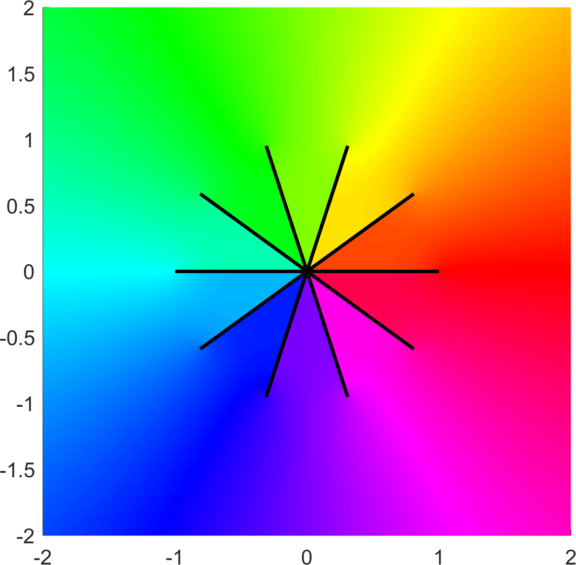
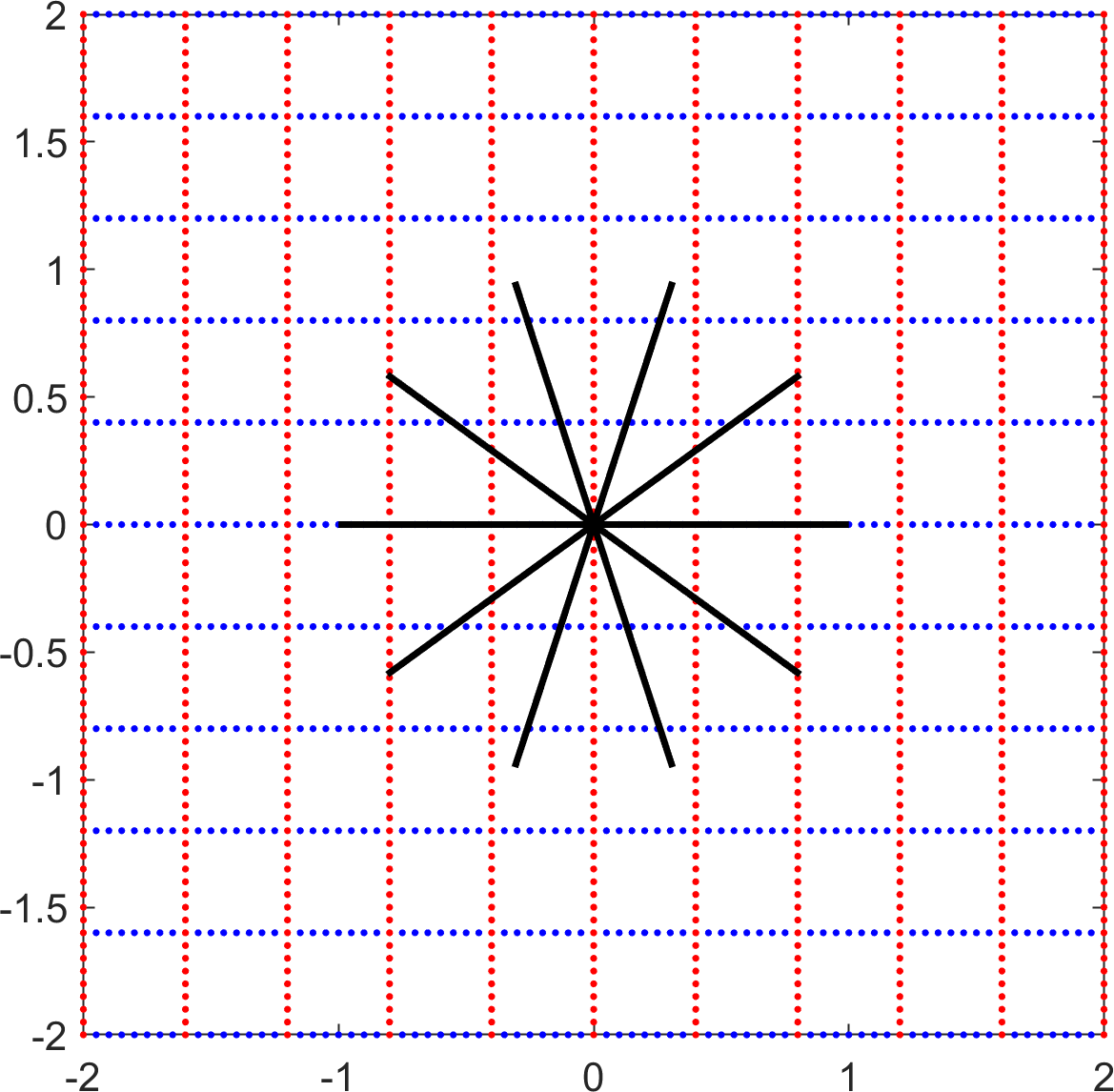
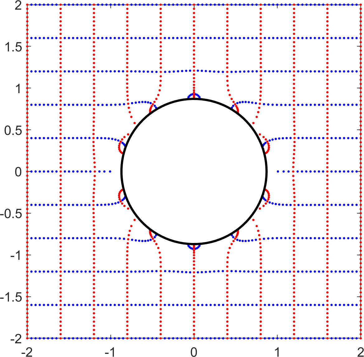
Figure 2: Pre-image $E=P^{-1}([-1,1])$ with $P(z)=z^{5}$ in Example 4.1. Left: Phase plot of $\Phi$, middle: $E$ (black) and grid, right: $\partial L$ (black) and image of the grid under $\Phi$.

Example 4.2.

Let $\Omega=\mathcal{E}_{1.25}$ be the Chebyshev ellipse bounded by $\{\frac{1}{2}(\frac{5}{4}e^{it}+\frac{4}{5}e^{-it}):t\in[0,2\pi[\}$ and let $E=P^{-1}(\mathcal{E}_{1.25})$ with $P(z)=(z-1)^{5}+\gamma$ for two different values of $\gamma$. For $\gamma=0.3i\notin\Omega$, the set $E$ consists of $n=5$ components, while for $\gamma=0.75\in\Omega$, the set $E$ has only one component; see Proposition 3.6. Figure 3 shows phase plots of $\Phi$ (left), the sets $\partial E$ and $\partial L$ in black and a grid and its image. The phase plots show $\Phi$ and an analytic continuation to the interior of $E$. The discontinuities in the phase (in the interior of $E$) are branch cuts of this analytic continuation.

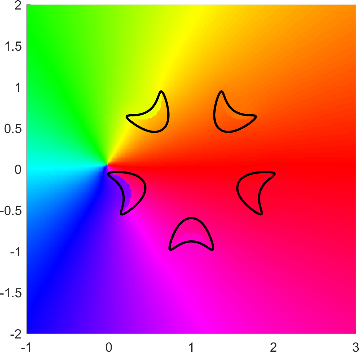
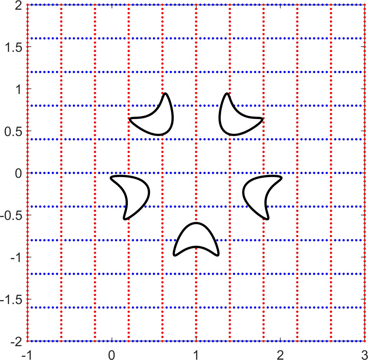
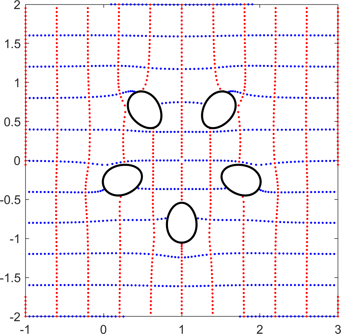
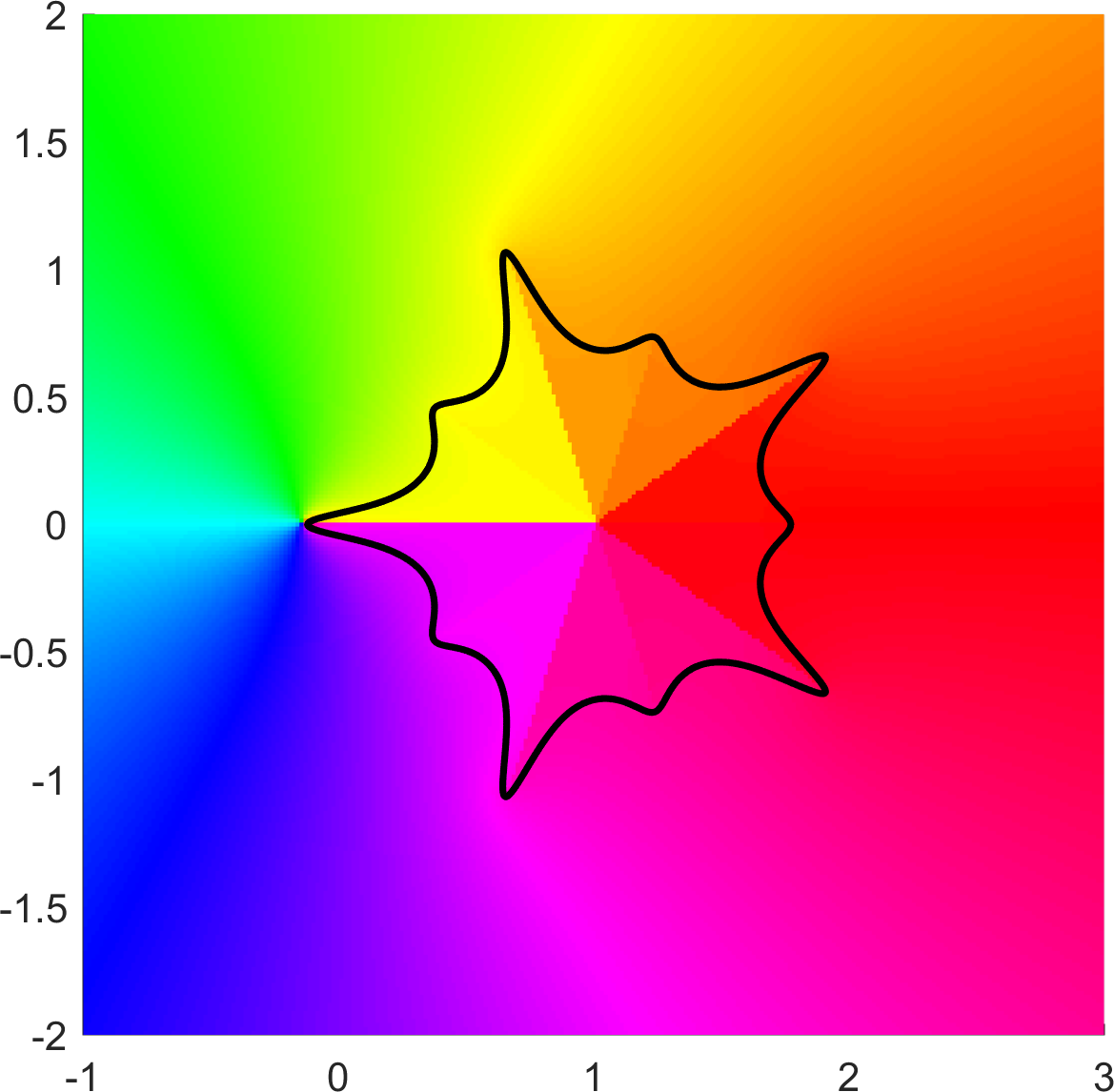
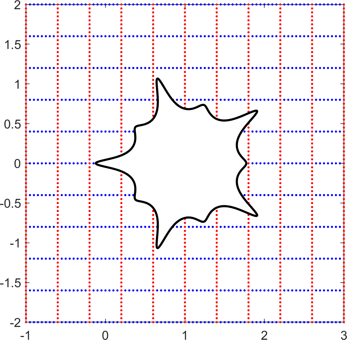
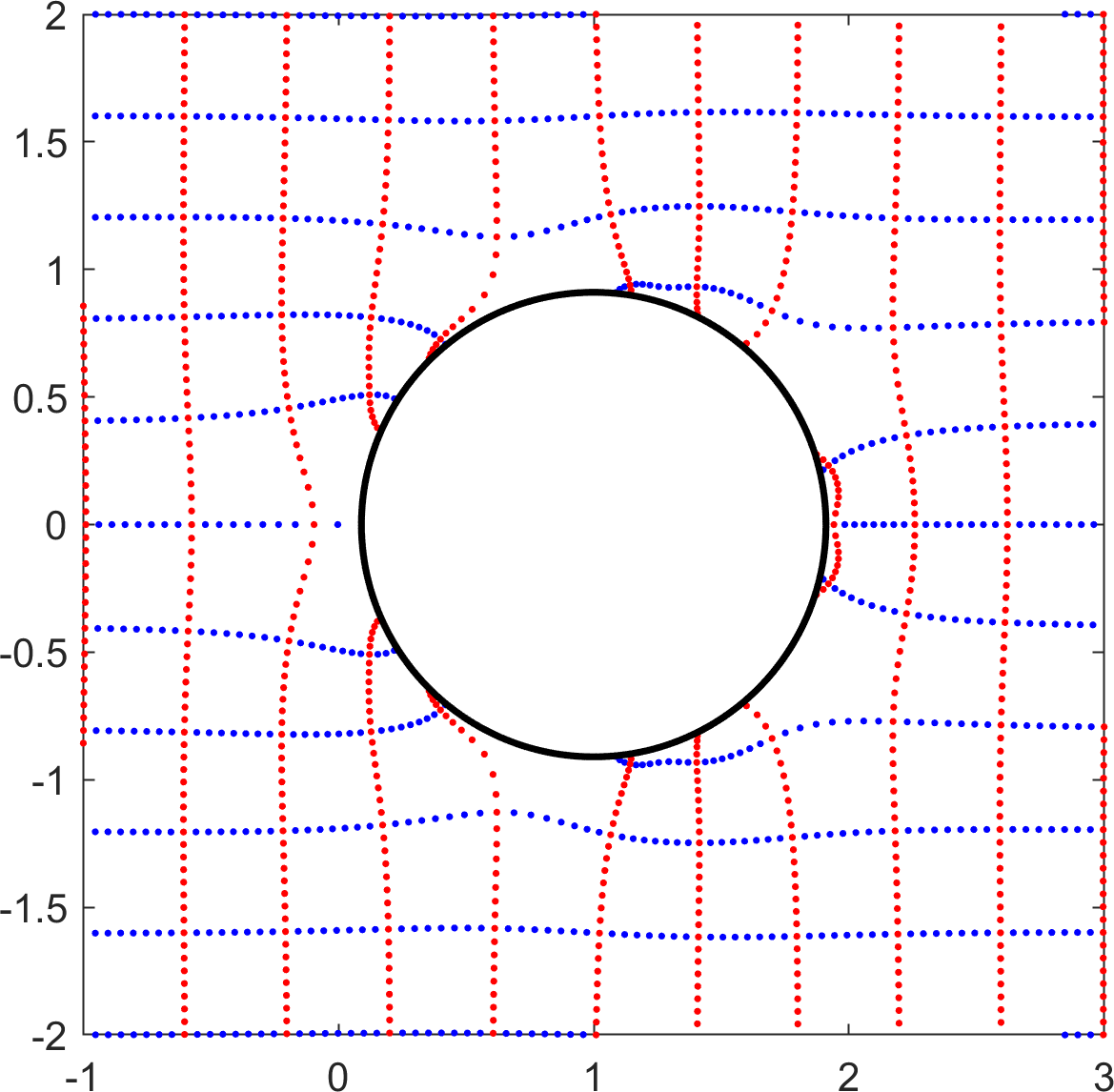
Figure 3: Set $E=P_{n}^{-1}(\Omega)$ with a Chebyshev ellipse $\Omega=\mathcal{E}_{1.25}$ and $P_{n}(z)=(z-1)^{5}+\gamma$, with $\gamma=0.3i\notin\Omega$ (top row) and $\gamma=0.75\in\Omega$ (bottom row); see Example 4.2. Phase plot of $\Phi$ (left), original and image domains with $\partial E$ and $\partial L$ in black (middle and right).

Example 4.3.

Let $P_{n}(z)=\alpha(z-\beta)^{n}+\gamma$ and $E=P_{n}^{-1}(\overline{\mathbb{D}})$.

1. If $\gamma\notin\overline{\mathbb{D}}$ then $\Phi(z)=z$ by Proposition 3.6, hence $L=E=\{z\in\mathbb{C}:\lvert P_{n}(z)\rvert\leq 1\}$, i.e., $E^{c}$ is a lemniscatic domain; see also Example 4.5 for pre-images of $\overline{\mathbb{D}}$ under general polynomials.

2. If $\gamma\in\overline{\mathbb{D}}$ then $E$ has only one component. In this case $\Phi(z)=z$ if and only if $\gamma=0$. Figure 4 shows an example with $\gamma\in\overline{\mathbb{D}}\setminus\{0\}$, where $E$ is not a lemniscatic domain and $\Phi(z)\neq z$.

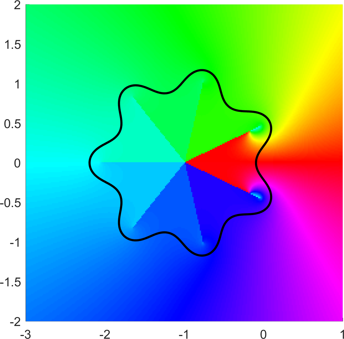
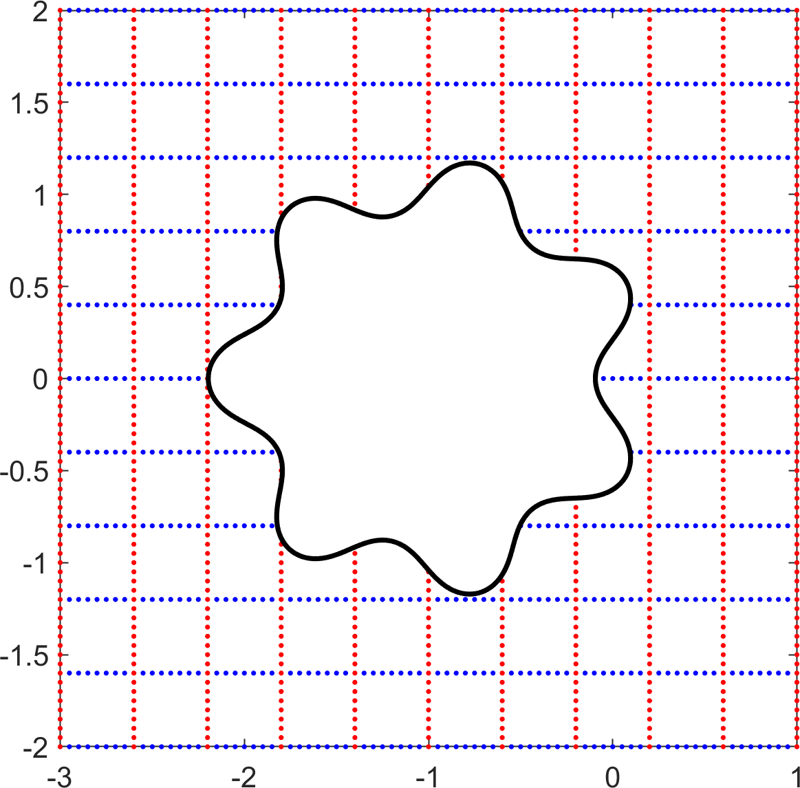
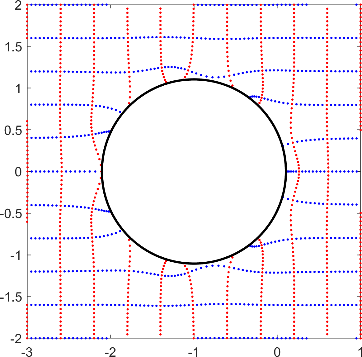
Figure 4: The set $E=P_{n}^{-1}(\overline{\mathbb{D}})$ with $P_{n}(z)=\frac{1}{2}(z+1)^{7}+\frac{3}{4}$. Phase plot of $\Phi$ (left), original and image domains with $\partial E$ and $\partial L$ in black (middle and right); see Example 4.3.

Next, we present an example for Corollary 3.7.

Example 4.4.

Consider the polynomial

$$P_{4}(z)=\frac{8z^{4}-8z^{2}+\alpha}{\alpha}$$

with $\alpha\geq 1$ from [11, Example (iv)]. Then $E=P_{4}^{-1}([-1,1])$ is connected, since the critical points of $P_{4}$ are $0,\pm 1/\sqrt{2}$ with corresponding critical values $P_{4}(0)=1\in[-1,1]$ and $P_{4}(\pm 1/\sqrt{2})=1-\frac{2}{\alpha}\in[-1,1]$; see Theorem 3.1. By Corollary 3.7,

$$L=\Bigg{\{}w\in\mathbb{C}:\lvert w\rvert\leq\operatorname{cap}(E)=\frac{\alpha^{1/4}}{2}\bigg{\}},$$

and the conformal map is

$$\Phi:E^{c}\to L^{c},\quad\Phi(z)=\frac{\sqrt[4]{\alpha}}{2}\sqrt[4]{P_{4}(z)+\sqrt{P_{4}(z)^{2}-1}},$$

see Figure 5. Since $E^{*}=E$, we have that $\Phi(z)=\overline{\Phi(\overline{z})}$ and, since $\Phi(z)=z+\mathcal{O}(1/z)$, we have in particular $\Phi(]1,\infty[)=]\operatorname{cap}(E),\infty[$ and $\Phi(]-\infty,-1[)=]-\infty,-\operatorname{cap}(E)[$. Since $E$ is also symmetric with respect to the imaginary axis, we similarly have $\Phi(]0,i\infty[)=]i\operatorname{cap}(E),i\infty[$ and $\Phi(]-i\infty,0[)=]-i\infty,-i\operatorname{cap}(E)[$. Hence, $\Phi$ maps each quadrant to itself. We use this to determine the correct branch of the fourth root.

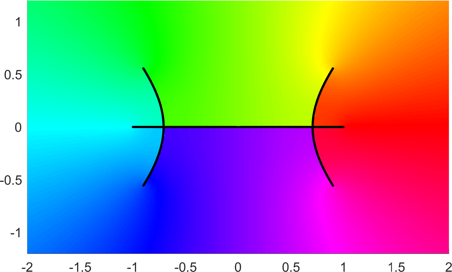
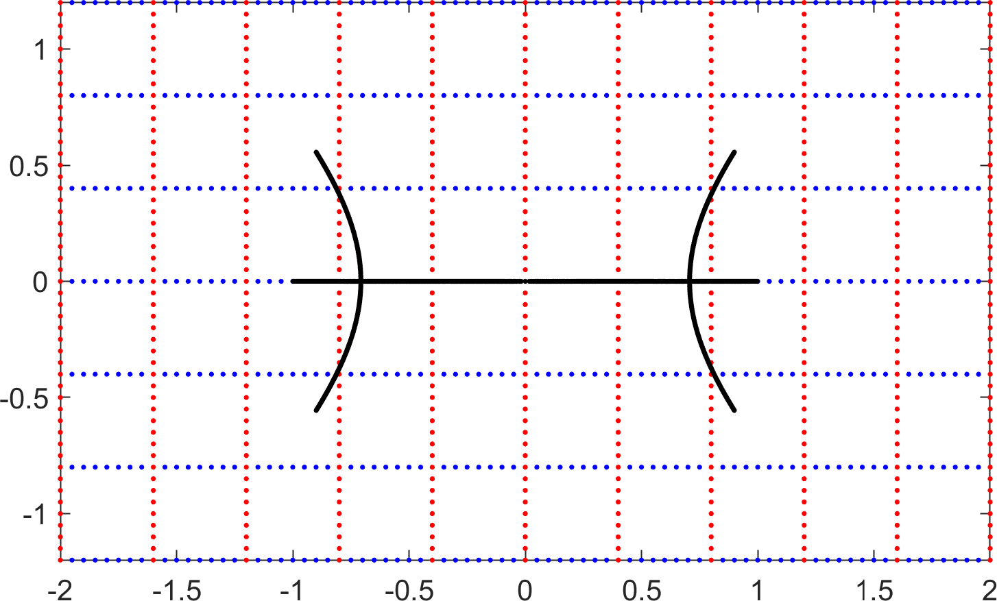
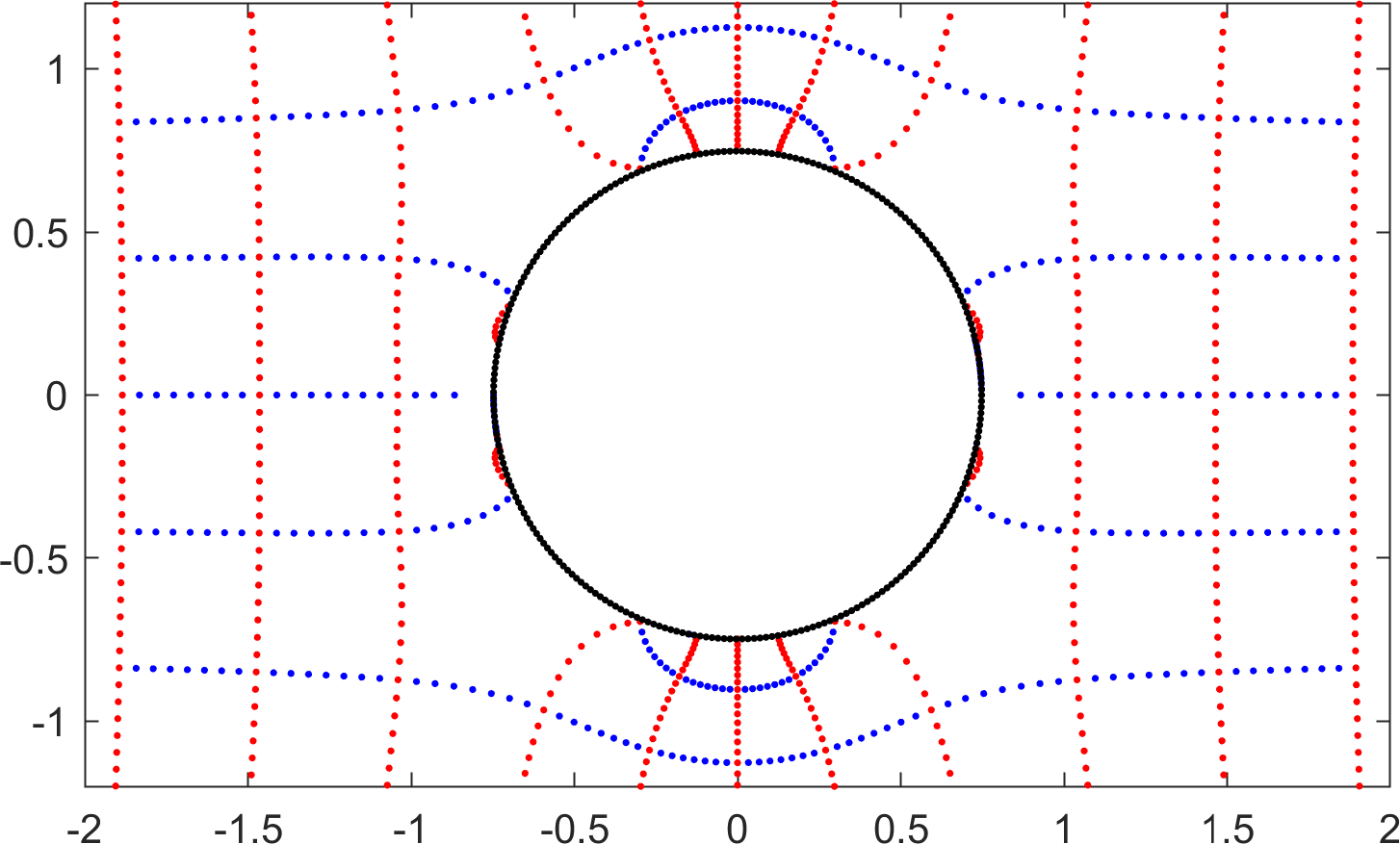
Figure 5: The set $E=P_{4}^{-1}([-1,1])$ with $\alpha=5$ in Example 4.4. Phase plot of $\Phi$ (left), original and image domains with $E$ and $\partial L$ in black (middle and right).

Example 4.5.

Let $P_{n}(z)=p_{n}\prod_{j=1}^{n}(z-b_{j})$ be a polynomial of degree $n$. If $E=P_{n}^{-1}(\overline{\mathbb{D}})$ consists of $n$ components then $E^{c}$ is a lemniscatic domain, i.e., $L=E$ with $a_{j}=b_{j}$, $m_{j}=1/n$, $\operatorname{cap}(E)=\lvert p_{n}\rvert^{-1/n}$, and $\Phi(z)=z$. Similarly, if $P_{n}(z)=p_{n}\prod_{j=1}^{\ell}(z-b_{j})^{n_{j}}$ with distinct $b_{1},\ldots,b_{\ell}\in\mathbb{C}$ and if $E$ has $\ell$ components, then $E^{c}$ is a lemniscatic domain, $L=E$ with $a_{j}=b_{j}$, $m_{j}=n_{j}/n$, and $\Phi(z)=z$.

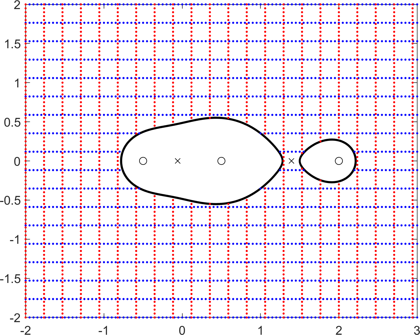
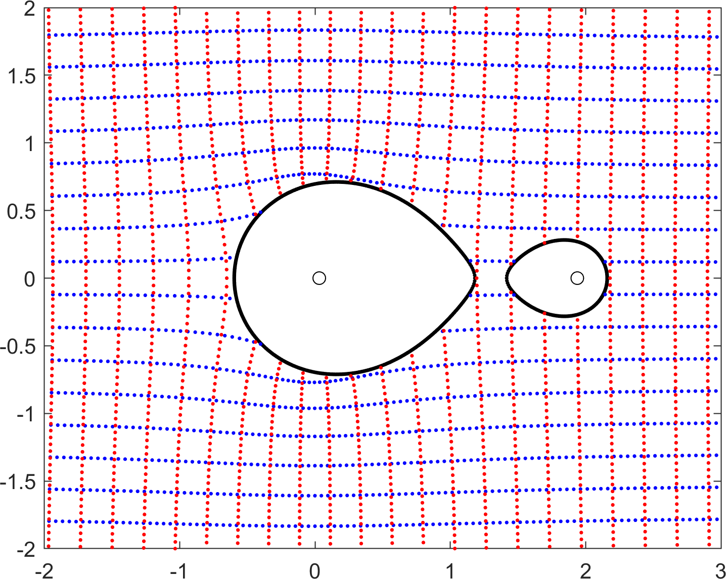
Figure 6: Pre-image $E=P_{3}^{-1}(\overline{\mathbb{D}})$ in Example 4.6. Left: $\partial E$ (black line), zeros of $P_{3}$ (circles) and $P_{3}^{\prime}$ (crosses), and a cartesian grid. Right: $\partial L$ (black line), $a_{1},a_{2}$ (circles) and the image of the grid under $\Phi$.

Finally, we consider an example for Theorem 3.8.

Example 4.6.

For $\alpha,\beta\in\mathbb{C}$, consider the polynomial

$$P_{3}(z)=(z-\alpha)(z^{2}-\beta^{2})=z^{3}-\alpha z^{2}-\beta^{2}z+\alpha\beta^{2}$$

of degree $n=3$. The critical points of $P_{3}$ are

$$z_{\pm}=\frac{\alpha\pm\sqrt{\alpha^{2}+3\beta^{2}}}{3}.$$

In the case $\alpha=2$ and $\beta=1/2$, we have $P_{3}(z_{-})\approx 0.5076\in\overline{\mathbb{D}}$ and $P_{3}(z_{+})\approx 1.9375\in\mathbb{C}\setminus\overline{\mathbb{D}}$, hence $E=P_{3}^{-1}(\overline{\mathbb{D}})$ has $\ell=2$ components by Theorem 3.1; see Figure 6 (left). Note that $E^{c}$ is not a lemniscatic domain (in contrast to the case considered in Example 4.5). Write $E=E_{1}\cup E_{2}$, where $E_{1}$ is the component on the left (with $\pm\beta\in E_{1}$). Then $m_{1}=2/3$ and $m_{2}=1/3$ by Theorem 3.2. Moreover, $E_{1}^{*}=E_{1}$ and $E_{2}^{*}=E_{2}$, since $P_{n}$ is real and $\overline{\mathbb{D}}$ is symmetric with respect to the real line, which implies that $a_{1},a_{2}\in\mathbb{R}$ by Theorem 2.7. Then, by Theorem 3.8,

$$\left(a_{2}-\frac{\alpha}{3}\right)^{3}=-2P_{3}(z_{+})\in\mathbb{R}.$$

Since $a_{2}-\frac{\alpha}{3}$ is real, taking the real third root yields

$$a_{2}=\frac{\alpha}{3}+\sqrt[3]{-2P_{3}(z_{+})}\approx 1.9375\quad\text{and}\quad a_{1}=\frac{1}{3}\alpha-\frac{1}{2}\sqrt[3]{-2P_{3}(z_{+})}\approx 0.0313.$$

Moreover, $\operatorname{cap}(E)=1$ by (3.8), hence

$$L=\{w\in\mathbb{C}:\lvert w-a_{1}\rvert^{2/3}\lvert w-a_{2}\rvert^{1/3}\leq 1\}.$$

Here, $Q(w)=(w-a_{1})^{2}(w-a_{2})^{1}$, hence

$$\Phi(z)=Q^{-1}(P_{3}(z)),$$

with a branch of $Q^{-1}$ such that $\Phi(z)=z+\mathcal{O}(1/z)$ at infinity. Here, we can obtain the boundary values of $\Phi$ for $z\in\partial E$ by solving $Q(w)=P_{3}(z)$ and identifying the boundary points in the correct way. Then, since $\Phi(z)-z$ is analytic in $E^{c}$ and zero at infinity, we have

$$\Phi(z)=z+\frac{1}{2\pi i}\int_{\partial E}\frac{\Phi(\zeta)-\zeta}{\zeta-z}\,d\zeta,\quad z\in\mathbb{C}\setminus E,$$ (4.1)

where $\partial E$ is negatively oriented, such that $E^{c}$ lies to the left of $\partial E$. Figure 6 also shows a cartesian grid (left) and its image under $\Phi$ (right). For the computation, we numerically approximate the integral in (4.1) with the trapezoidal rule.

Appendix A Appendix

Lemma A.1.

Let $E\subseteq\mathbb{C}$ be compact, such that $E^{c}$ has a Green’s function $g_{E}$. If $E^{*}=E$, then $g_{E}(\overline{z})=g_{E}(z)$ and $\partial_{z}g_{E}(\overline{z})=\overline{\partial_{z}g_{E}(z)}$. Moreover, the critical points of $g_{E}$ are real or appear in complex conjugate pairs.

Proof.

Since $E^{*}=E$, the function $z\mapsto g_{E}(\overline{z})$ is also a Green’s function with pole at infinity of $E^{c}$, hence $g_{E}(\overline{z})=g_{E}(z)$ for all $z\in E^{c}$ by the uniqueness of the Green’s function. Write $g(x,y)=g_{E}(z)$, then $g(x,y)=g(x,-y)$ and

$$\frac{\partial g}{\partial x}(x,y)=\frac{\partial g}{\partial x}(x,-y),\quad\frac{\partial g}{\partial y}(x,y)=-\frac{\partial g}{\partial y}(x,-y),$$ (A.1)

hence

$$2\partial_{z}g_{E}(z)=\frac{\partial g}{\partial x}(x,y)-i\frac{\partial g}{\partial y}(x,y)=\frac{\partial g}{\partial x}(x,-y)+i\frac{\partial g}{\partial y}(x,-y)=\overline{2(\partial_{z}g_{E})(\overline{z})}.$$

The critical points of $g_{E}$ are the zeros of the analytic function $\partial_{z}g_{E}$. Since $\partial_{z}g_{E}(\overline{z})=\overline{\partial_{z}g_{E}(z)}$, if $z_{*}$ is a zero of $\partial_{z}g_{E}$ then also $\overline{z}_{*}$ is a zero. ∎

Lemma A.2.

Let $K\subseteq\mathbb{C}$ be a non-empty compact, simply connected set with $K^{*}=K$, then $K\cap\mathbb{R}$ is either an interval or a single point.

Proof.

Since $K^{*}=K$ and $K$ is connected, $K\cap\mathbb{R}$ is not empty. Since $K^{c}$ is connected, $K\cap\mathbb{R}$ must be connected (otherwise the symmetry and simply-connectedness of $K$ would imply that $K^{c}$ is not connected). Thus, $K\cap\mathbb{R}$ is a point or an interval. ∎

Lemma A.3.

Let $\gamma$ be a smooth Jordan curve symmetric with respect to the real line and let $f$ be integrable with $f(\overline{z})=\overline{f(z)}$ on $\gamma$. Then

$$\frac{1}{2\pi i}\int_{\gamma}f(z)\,dz\in\mathbb{R}.$$

Proof.

Since $\gamma$ is symmetric with respect to the real line, we can write $\gamma=\gamma_{1}+\gamma_{2}$ with $\gamma_{2}\coloneq-\overline{\gamma}_{1}$. Then

$$\begin{split}\int_{\gamma}f(z)\,dz&=\int_{\gamma_{1}}f(z)\,dz-\int_{\overline{\gamma}_{1}}f(z)\,dz=\int_{a}^{b}f(\gamma_{1}(t))\cdot\gamma_{1}^{\prime}(t)\,dt-\int_{a}^{b}f(\overline{\gamma_{1}(t)})\cdot\overline{\gamma_{1}^{\prime}(t)}\,dt\\ &=2i\int_{a}^{b}\operatorname{Im}(f(\gamma_{1}(t))\cdot\gamma_{1}^{\prime}(t))\,dt,\end{split}$$

which yields the result. ∎

Though the following theorem must be known, we did not find it in the literature. For completeness, we include a proof.

Theorem A.4.

Let $P$ be a non-constant polynomial and $\Omega\subseteq\mathbb{C}$ be a simply connected compact set. Then $\widehat{\mathbb{C}}\setminus P^{-1}(\Omega)$ is open and connected, i.e., a region.

Proof.

Clearly, $G\coloneq\widehat{\mathbb{C}}\setminus P^{-1}(\Omega)=P^{-1}(\widehat{\mathbb{C}}\setminus\Omega)$ is open and contains $\infty$. Let $G_{\infty}\subseteq G$ be that component of $G$ that contains $\infty$. Suppose that $G$ is not connected, i.e., $G\neq G_{\infty}$. Then there exists another component $G_{1}\subseteq G$, and $G_{1}$ is a bounded region. Then $P(G_{1})$ is a bounded region with $P(G_{1})\subseteq\widehat{\mathbb{C}}\setminus\Omega$.

Next, we show that $\partial P(G_{1})\subseteq\partial\Omega$. Let $w\in\partial P(G_{1})$. Then there exists $w_{k}\in P(G_{1})$ with $w_{k}\to w$. For each $k$, there exists $z_{k}\in G_{1}$ with $P(z_{k})=w_{k}$. Since $G_{1}$ is bounded, the sequence $(z_{k})_{k}$ has a convergent subsequence $(z_{k_{j}})_{j}$ with $z_{k_{j}}\to z\in\overline{G}_{1}$. This implies that $P(z)=w$. Since $w\in\partial P(G_{1})$, we have $z\in\partial G_{1}$ (otherwise, $z\in G_{1}$ would imply $P(z)\in P(G_{1})$ and, since $P(G_{1})$ is open, $w=P(z)\notin\partial P(G_{1})$). Since $G$ is open, this implies that $z\notin G$ and hence that $z\in P^{-1}(\Omega)$ and $w=P(z)\in\Omega$. Since $w_{k}\in P(G_{1})\subseteq\widehat{\mathbb{C}}\setminus\Omega$ and $w_{k}\to w$, we obtain that $w\in\partial\Omega$.

We have shown that $P(G_{1})\subseteq\widehat{\mathbb{C}}\setminus\Omega$ is a region with $\partial P(G_{1})\subseteq\partial\Omega=\partial(\widehat{\mathbb{C}}\setminus\Omega)$. Since $\widehat{\mathbb{C}}\setminus\Omega$ is connected, this implies that $P(G_{1})=\widehat{\mathbb{C}}\setminus\Omega$, which contradicts that $P(G_{1})$ is bounded. This shows that $G=\widehat{\mathbb{C}}\setminus P^{-1}(\Omega)$ is connected. ∎

References

[1]L. V. Ahlfors, Complex analysis: An introduction of the theory of
analytic functions of one complex variable, third edition, McGraw-Hill Book
Co., New York-Toronto-London, 1979.
[2]H. Grunsky, Über konforme Abbildungen, die gewisse
Gebietsfunktionen in elementare Funktionen transformieren. I, Math.
Z., 67 (1957), pp. 129–132.
[3], Über konforme
Abbildungen, die gewisse Gebietsfunktionen in elementare Funktionen
transformieren. II, Math. Z., 67 (1957), pp. 223–228.
[4], Lectures on theory
of functions in multiply connected domains, Vandenhoeck & Ruprecht,
Göttingen, 1978.
Studia Mathematica, Skript 4.
[5]J. A. Jenkins, On a canonical conformal mapping of J. L.
Walsh, Trans. Amer. Math. Soc., 88 (1958), pp. 207–213.
[6]H. J. Landau, On canonical conformal maps of multiply connected
domains, Trans. Amer. Math. Soc., 99 (1961), pp. 1–20.
[7]A. I. Markushevich, Theory of functions of a complex variable.
Vol. I, Translated and edited by Richard A. Silverman, Prentice-Hall,
Inc., Englewood Cliffs, N.J., 1965.
[8]M. M. S. Nasser, J. Liesen, and O. Sète, Numerical computation of
the conformal map onto lemniscatic domains, Comput. Methods Funct. Theory,
16 (2016), pp. 609–635.
[9]T. Ransford, Potential theory in the complex plane, vol. 28 of
London Mathematical Society Student Texts, Cambridge University Press,
Cambridge, 1995.
[10]K. Schiefermayr, Geometric properties of inverse polynomial images,
in Approximation theory XIII: San Antonio 2010, vol. 13 of Springer
Proc. Math., Springer, New York, 2012, pp. 277–287.
[11], The
Pólya-Chebotarev problem and inverse polynomial images, Acta Math.
Hungar., 142 (2014), pp. 80–94.
[12]O. Sète and J. Liesen, On conformal maps from multiply connected
domains onto lemniscatic domains, Electron. Trans. Numer. Anal., 45 (2016),
pp. 1–15.
[13]J. L. Walsh, On the conformal mapping of multiply connected
regions, Trans. Amer. Math. Soc., 82 (1956), pp. 128–146.
[14], A generalization of
Faber’s polynomials, Math. Ann., 136 (1958), pp. 23–33.
[15], Interpolation and
approximation by rational functions in the complex domain, Fifth edition.
American Mathematical Society Colloquium Publications, Vol. XX, American
Mathematical Society, Providence, R.I., 1969.